ANALYSIS AND MODELING OF COUPLED THERMO-HYDRO

UNIVERSIDAD POLITÉCNICA DE MADRID

ESCUELA TÉCNICA SUPERIOR DE INGENIEROS DE MINAS

ANALYSIS AND MODELING OF COUPLED THERMO-HYDRO-

MECHANICAL PHENOMENA IN 3D FRACTURED MEDIA

(Análisis y Modelización de Fenómenos Acoplados Termo-Hidro-Mecánicos en Medio Fracturado)

TESIS DOCTORAL

ISRAEL CAÑAMÓN VALERA Ingeniero de Minas

2006

N° d’ordre :………………

THESE

présentée pour obtenir

LE TITRE DE DOCTEUR DE L’INSTITUT NATIONAL POLYTECHNIQUE DE

TOULOUSE

École doctorale : Sciences de l’Univers de l’Environnement et de l’Espace Spécialité : Sciences de la terre et environnement

Par M…Israel CAÑAMON VALERA

Titre de la thèse

ANALYSE ET MODELISATION DES PHENOMENES COUPLES THERMO-HYDRO-MECANIQUES EN MILIEUX FRACTURES 3D

Soutenue le 30/11/2006 devant le jury composé de :

M. Prof. Dr.-Ing. Ghislain de MARSILY Rapporteur M. Prof. Dr.-Ing. Jesus CARRERA Rapporteur M. Prof. Dr.-Ing. Pedro R. OYANGUREN Membre M. DR CNRS Dr.-Ing. Michel QUINTARD Membre M. DR CNRS Dr. Alain MANGIN Membre M. Prof. Dr.-Ing. Rachid ABABOU Directeur M. Prof. Dr.-Ing. Fco. Javier ELORZA Directeur M. Prof. Dr.-Ing. Philippe RENARD Invité

DEPARTAMENTO DE MATEMÁTICA APLICADA Y MÉTODOS INFORMÁTICOS

ESCUELA TÉCNICA SUPERIOR DE INGENIEROS DE MINAS

ANALYSIS AND MODELING OF COUPLED THERMO-HYDRO-

MECHANICAL PHENOMENA IN 3D FRACTURED MEDIA

Author: ISRAEL CAÑAMÓN VALERA Ingeniero de Minas

Directors: FRANCISCO JAVIER ELORZA TENREIRO Dr. Ingeniero de Minas

RACHID ABABOU Dr.-Ing. Mécanique des Fluides, Ph.D. Civil Engineering

2006

(D-15)

de la Universidad

Tribunal nombrado por el Magfco. Y Excmo. Sr. Rector

Politécnica de Madrid, el día ………….. de ………….. de 200……..

Presidente: .

Vocal: .

Vocal: .

Vocal: .

Secretario: .

Suplente: .

Suplente: .

ealizado el acto de la defensa y lectura de la Tesis el día …… de …………... de 200…

n la E.T.S.I. / Facultad ……………………………………………….

L PRESIDENTE LOS VOCALES

EL SECRETARIO

R

e

E

UNIVERSIDAD POLITÉCNICA DE MADRID

To my wife, Veracruz.

IX

ACKNOWLEDGEMENTS This work is part of the research of the FEBEX I and II projects, co-funded by ENRESA and the European Commission under contract numbers FI4W-CT95-0006 and FIKW-CT-2000-0016 of the IV and V Mark Programs respectively. I would like to thank specially my two thesis directors, Fco. Javier Elorza and Rachid Ababou, for all the personal and scientific support that have given to me during the thesis studies. I would like to thank, also, all the outstanding professors and researchers that have helped me in specific topics at some point during the research, and excusing myself if I forget someone in the list: Alain Mangin, Carlos Paredes, Ruxandra Nita, Enrique Chacón, Ángel Udías, Ramón Rodríguez, Ultano Kindelán, Santiago de Vicente, Fernando Huertas, Pascual Farias, etc. And thanks to the Departamento de Matemática Aplicada y Métodos Informáticos of the E.T.S.I.M. and its staff to give me the opportunity to accomplish my doctoral studies within its framework.

XI

ABSTRACT

Analysis and Modeling of Coupled Thermo-Hydro-Mechanical Phenomena in 3D Fractured Media.

This doctoral research was conducted as part of a joint France-Spain « cotutelle » PhD thesis in the framework of a bilateral agreement between two universities, the Institut National Polytechnique de Toulouse (INPT) and the Universidad Politecnica de Madrid (UPM). It concerns a problem of common interest at the national and international levels, namely, the disposal of radioactive waste in deep geological repositories. The present work is devoted, more precisely, to near-field hydrogeological aspects involving mass and heat transport phenomena. The first part of the work is devoted to a specific data interpretation problem (pressures, relative humidities, temperatures) in a multi-barrier experimental system at the scale of a few meters – the “Mock-Up Test” of the FEBEX project, conducted in Spain. Over 500 time series are characterized in terms of spatial, temporal, and/or frequency/scale-based statistical analysis techniques. The time evolution and coupling of physical phenomena during the experiment are analyzed, and conclusions are drawn concerning the behavior and reliability of the sensors. The second part of the thesis develops in more detail the 3-Dimensional (3D) modeling of coupled Thermo-Hydro-Mechanical phenomena in a fractured porous rock, this time at the scale of a hundred meters, based on the data of the “In-Situ Test” of the FEBEX project conducted at the Grimsel Test Site in the Swiss Alps. As a first step, a reconstruction of the 3D fracture network is obtained by Monte Carlo simulation, taking into account through optimization the geomorphological data collected around the FEBEX gallery. The heterogeneous distribution of traces observed on the cylindrical wall of the tunnel is fairly well reproduced in the simulated network. In a second step, we develop a method to estimate the equivalent permeability of a many-fractured block by extending the superposition method of Ababou et al. [1994] to the case where the permeability of the rock matrix is not negligible (matrix permeability may embody some finer fracturing in addition to pore space). When fracture flow is complemented by significant matrix permeability, it may be possible to avoid empirical connectivity-based corrections, which are used in the literature to account for non-percolation effects. The superposition approach is also applied here to coupled Hydro-Mecanical problems to obtain the equivalent coefficients of the 3D fractured medium, including the permeability tensor, but also elastic stiffness or compliance coefficients, as well as pressure-strain coupling coefficients (Biot). Finally, these results are used to develop a continuum equivalent model for 3D coupled Thermo-Hydro-Mechanics, including: hydro-mechanical coupling via tensorial Biot equations (non-orthotropic), a darcian flow in an equivalent porous medium (anisotropic permeability), as well as thermal stresses and heat transport by diffusion and convection, taking into account the thermal expansivity of water. Transient simulations of the excavation of the FEBEX gallery, and of the heating due to hypothetical radioactive waste canisters, are conducted using the Comsol Multiphysics ® software (3D finite elements). The results of numerical simulations are analyzed for different cases and different ways of stressing the system. Finally, preliminary comparisons of simulations with time series data collected during the “In-Situ Test” of FEBEX yield encouraging results.

XIII

RÉSUMÉ

Analyse et modélisation des phénomènes couplés Thermo-Hydro-Mécaniques en milieux fracturés 3D.

Ce mémoire présente un travail de thèse conduite en cotutelle France-Espagne dans le cadre d'une convention entre l'Institut National Polytechnique de Toulouse (INPT) et l'Université Polytechnique de Madrid (UPM). Il porte sur un problème d'intérêt commun au niveau national et international, le stockage de déchets radioactifs en milieux géologiques profonds. Le mémoire est consacré plus particulièrement aux aspects hydrogéologiques et aux transferts de masse et de chaleur en champ proche. Dans une première partie, on s'intéresse à un problème particulier d'interprétation de données (pressions, humidités relatives, températures) dans une expérience de systèmes multi-barrières à l'échelle de quelques mètres - le « Test Mock-up » du projet FEBEX réalisé en Espagne. Des techniques d’analyse statistique spatiale, temporelle et de fréquence / échelle sont appliquées à plus de 500 chroniques de données. On analyse le déroulement et le couplage des phénomènes physiques qui ont eu lieu lors de l’expérience, et on tire des conclusions sur le comportement et la fiabilité des capteurs. La seconde partie de la thèse développe plus en détail la modélisation des phénomènes Thermo-Hydro-Mécaniques 3-Dimensionnels (3D) dans une roche poreuse fracturée, cette fois-ci à l'échelle de la centaine de mètres, en s'appuyant sur les données du « Test In-Situ » du projet FEBEX, réalisé au Grimsel Test Site dans les Alpes Suisses. En première étape, une reconstruction 3D du réseau de fractures est réalisée par simulation de Monte-Carlo en tenant compte, par optimisation, des données géomorphologiques collectées autour de la galerie FEBEX. La distribution hétérogène de traces observée sur la paroi cylindrique de la galerie est assez bien reproduite dans le réseau simulé. Dans une seconde étape, on développe une méthode pour estimer la perméabilité équivalente d’un bloc multi-fracturé en généralisant la méthode de superposition de Ababou et al. [1994] au cas où la perméabilité matricielle est non négligeable (celle-ci peut représenter non seulement l’espace poral mais aussi une fracturation fine). Avec la perméabilité matricielle, il devient envisageable d’éviter les corrections empiriques basées sur la connectivité, qui sont employées dans la littérature pour tenir compte des effets de non-percolation. L’approche « superposition » est également appliquée ici au problème couplé hydro-mécanique afin d’obtenir les coefficients équivalents du milieu fracturé 3D, qui comprennent (outre le tenseur de perméabilité) les coefficients tensoriels de raideur ou de complaisance élastique, et des coefficients de couplage pression-déformation (Biot). Finalement, à partir de ces résultats, on réalise un modèle thermo-hydro-mécanique couplé en milieu continu équivalent 3D, comprenant : des couplages hydro-mécaniques par les équations tensorielles de Biot (non orthotrope), un flux darcien dans le milieu poreux équivalent (perméabilité anisotrope), ainsi que des contraintes thermiques et du transport de chaleur par diffusion et convection tenant compte de l’expansivité thermique du fluide. Des simulations transitoires de l’excavation de la galerie FEBEX et du réchauffement provoqué par l’éventuel stockage de colis de déchets radioactifs sont conduites à l’aide du logiciel numérique Comsol Multiphysics ® (éléments finis 3D). Les résultats de simulation sont analysés dans différents cas et pour différents types de sollicitations. Enfin, les premières comparaisons des simulations numériques avec les chroniques de données provenant du « Test In-Situ » FEBEX donnent des résultats encourageants.

XV

RESUMEN

Analisis y Modelización de Fenómenos Acoplados Termo-Hidro-Mecánicos en Medios Fracturados 3D.

Esta tesis doctoral surge como resultado de un convenio de cotutela en el marco de un acuerdo bilateral entre la Universidad Politécnica de Madrid (UPM) y el Institut National Polytechnique de Toulouse (INPT). Trata un asunto de interés tanto nacional como internacional como es el almacenamiento de residuos radiactivos en almacenamientos geológicos profundos de tipo granítico. El presente trabajo se ocupa, en concreto, de los aspectos hidrogeológicos en el campo cercano, en los que los fenómenos de transporte de calor y de masa son predominantes. La primera parte de la tesis se ocupa del analisis de series temporales (presiones, humedades relativas, temperaturas, etc) en un sistema multibarrera a escala de unos metros – el ensayo “en Maqueta” del proyecto FEBEX, llevado a cabo en las instalaciones del CIEMAT. Más de 500 series temporales son caracterizadas mediante técnicas de análisis estadístico en los dominios espacial, temporal y de frecuencia / escala. Se analiza la evolución temporal y las correlaciones entre los distintos fenómenos físicos a lo largo del ensayo, así como el comportamiento y la fiabilidad de los sensores. La segunda parte de la tesis desarrolla la modelización tridimiensional de fenómenos acoplados Termo-Hidro-Mecánicos (THM) en medios porosos fracturados, en este caso a escala de la centena de metros, a partir de los datos del experimento “In-situ” del proyecto FEBEX, llevado a cabo en el Laboratorio Subterráneo de Grimsel en los alpes suizos. En una primera etapa se realiza la reconstrucción de la red de fracturas en tres dimensiones mediante una simulación de Montecarlo, que tiene en cuenta los estudios geomorfológicos llevados a cabo alrededor de la galería FEBEX mediante un algoritmo de optimización. Esta simulación es capaz de reproducir la distribución heterogénea de trazas observada en el muro de la galería cilíndrica con precisión. En una segunda etapa, se desarrolla una extensión del método de superposición de [5] para estimar la permeabilidad equivalente de múltiples bloques fracturados para el caso en el que la permeabilidad de la matriz rocosa no es despreciable (la permeabilidad de la matriz rocosa puede también incluir el efecto de una microfisuración). Cuando el flujo a través de la red de fracturas se complementa con una permeabilidad en la matriz rocosa, es posible evitar las correcciones empíricas basadas en la conectividad que otros autores emplean para tener en cuenta los efectos de la no-percolación. Dicho método de superposición se aplica también al problema hidro-mecánico para calcular el resto de coeficientes equivalentes del medio fracturado 3D, como son el tensor de rigidez y los tensores de los coeficientes de acoplamiento presion-deformación (Biot). Finalmente, estos resultados son utilizados para desarrollar un modelo continuo equivalente con acoplamiento Termo-Hidro-Mecánico en tres dimensiones, que incluye: acoplamiento hidro-mecánico vía las ecuaciones tensoriales de Biot (caso no-ortótropo), flujo de Darcy en un medio poroso equivalente (caso de permeabilidad anisótropa), esfuerzos térmicos y transporte de calor por difusión y convección, en el que se tiene en cuenta la expansividad térmica del agua. Se implementa el modelo en el programa de elementos finitos Comsol Multiphysics ® y se realizadan diversas simulaciones de la excavación de la galería FEBEX y del calentamiento producido por un hipotético almacenamiento de residuos radiactivos. Los resultados de estas simulaciones se analizan para distintos casos y distintas condiciones tensionales. Las comparaciones preliminares de los resultados de las simulaciones con las series de datos del experimento FEBEX “In-situ” auguran un buen ajuste del modelo.

XVII

RESUMEN EXTENDIDO

Analisis y Modelización de Fenómenos Acoplados Termo-Hidro-Mecánicos en Medios Fracturados 3D.

Introducción. La presente tesis se planteó como un ambicioso proyecto en el que se pretendía combinar las capacidades del análisis estadístico de datos con su aplicación para la elaboración de un modelo acoplado tridimensional del medio rocoso, todo ello en el marco del proyecto de ENRESA denominado “FEBEX”, sobre la simulación de un almacenamiento de residuos radiactivos. Los estudios estadísticos pretendían, así, arrojar luz sobre los fenómenos físicos y químicos fundamentales que ocurrían en un experimento de este tipo, en el que se combinan fenómenos térmicos, mecánicos y de transporte de fluido intersticial a través de distintos materiales y medios. Así mismo, pretendían servir de alimentación para elaborar un modelo acoplado termo-hidro-mecánico en tres dimensiones del medio fracturado que rodea dicho experimento. En la parte de análisis estadístico de datos se ha conseguido aplicar con éxito tanto técnicas clásicas de análisis de series temporales (correlación, análisis espectral) como otras más novedosas en este ámbito (ondeletes, matching pursuit). A la complejidad de las técnicas de análisis se ha unido la dificultad añadida de trabajar con bases de datos enormes (500 sensores, señales con más de 85.000 datos cada una), no sólo por el coste computacional del tiempo de análisis y por la gestión y postproceso de la información, sino también por la necesidad de interrelacionar un gran número de variables entre sí en el tiempo y en el espacio. No obstante, este tratamiento estadístico ha permitido identificar la importancia relativa de determinados procesos físicos con respecto a otros, así como también establecer unas bases para el futuro modelo acoplado en cuanto a variables relevantes y fenómenos constitutivos en este tipo de experimentos. Un resultado derivado, aunque no menos valioso, ha sido la identificación de señales espurias y erróneas dentro del proceso de toma de datos experimentales, que a simple vista y sin la ayuda de estas técnicas de análisis hubieran pasado desapercibidas. Por otro lado, en la parte de modelización, se ha desarrollado una metodología completa para el tratamiento y modelado de materiales fracturados mediante la simulación optimizada del medio y su posterior homogeneización a un medio continuo equivalente, más fácil de tratar de cara a los métodos numéricos que resuelven las ecuaciones del modelo. La reconstrucción del medio fracturado en base a datos geológicos experimentales ha resultado particularmente fructífera e innovadora, ya que un elemento totalmente novedoso en esta reconstrucción ha sido la utilización de cartografías de trazas de fracturas sobre las paredes de una galería cilíndrica (frente al empleo clásico de datos de trazas sobre una pared plana). Esto nos ha imposibilitado aprovechar la existencia de programas específicos que realizan esta tarea, y hemos desarrollado nuestro propio código de generación del medio fracturado y su optimización mediante el método de Montecarlo. Otro aspecto relevante de este apartado de reconstrucción del medio ha sido la adaptación del proceso de generación para reflejar la no uniformidad local dentro del mapa de trazas en cuando a la densidad de fracturación, conservando sin embargo una cierta uniformidad estadística en aquellas zonas del dominio donde no se poseía información geológica. De esta forma ha sido posible dar cuenta de la geometría local alrededor de la galería experimental (de vital importancia de cara al modelo) sin perder la generalidad regional en el comportamiento hidrogeológico del

XIX

macizo rocoso. También cabe destacar en esta segunda parte de la tesis varios aspectos relacionados con el propio modelo acoplado termo-hidro-mecánico. Se ha mejorado y completado la técnica de homogeneización definida en [5], y se han desarrollado de manera rigurosa las ecuaciones macroscópicas que incorporan intrínsecamente los acoplamientos hidro-mecánicos (ecuaciones de Biot, ley de Darcy, etc). Descripción del Proyecto FEBEX. El FEBEX es un proyecto de investigación en el ámbito de la gestión de residuos coordinado por ENRESA y cofinanciado por la Comisión Europea (EC). En él participan otros siete socios de tres países de la UE (Francia, Alemania y España) y uno de la EFTA (Suiza). El propósito del FEBEX (Full-scale Engineering Barriers Experiment in crystalline host rock) [45] es el estudio del comportamiento de componentes del campo próximo de un almacenamiento de residuos radiactivos de alta actividad (RRAA) en roca cristalina. El experimento consta de tres partes principales: 1) un ensayo “in situ”, en condiciones naturales y escala real; 2) un ensayo en “maqueta” realizado en CIEMAT, a escala casi real; 3) un conjunto de ensayos de laboratorio para complementar la información de los dos ensayos a gran escala. El experimento está basado en el concepto de almacenamiento español en roca cristalina: las cápsulas con el residuo se depositan horizontalmente en galerías, rodeadas por una barrera de arcilla formada por bloques fabricados con bentonita compactada a alta densidad. Análisis de Series Temporales del Ensayo en Maqueta. El comportamiento de un almacenamiento de RRAA debe estar determinado, en gran medida, por los procedimientos de diseño y construcción de la barrera de ingeniería y especialmente por los cambios que pueden producirse en sus propiedades mecánicas, hidráulicas y geoquímicas debidos a los efectos combinados del calor generado por desintegración radiactiva y al aporte de agua y de solutos desde la roca de alojamiento. Se considera, por tanto, fundamental comprender y cuantificar los procesos que tienen lugar en el campo próximo para evaluar el comportamiento a largo plazo del almacenamiento. Se ha llevado a cabo un análisis estadístico de las series de datos registradas en el ensayo en Maqueta a lo largo del experimento de hidratación/calentamiento con el fin de establecer las posibles relaciones entre los distintos procesos físicos.

Descripción de los datos. Un total de 486 señales se registran automáticamente con un intervalo de 30 min. en el experimento en “maqueta” del FEBEX, y otras 19 señales son grabadas de forma periódica por los operadores. Todas estas series corresponden a los sensores instalados en el interior de la estructura de confinamiento, en la bentonita o incorporados al calentador, así como los sensores externos e instrumentos. La estructura de la maqueta, cilindro horizontal de 6m de largo por 1,62m de diámetro, se divide en dos zonas, zona A y zona B (cada una con un calentador) divididas en 12 secciones respectivamente más una sección central entre ambas. Los sensores se encuentran localizados a lo largo de las 25 secciones transversales en que se divide la bentonita. Dentro de cada sección, se han definido cuatro niveles a diferentes distancias radiales del centro, y a su vez en cada nivel se distinguen ocho posiciones angulares a 45º.

XX

Metodologías de Análisis. El Análisis Correlatorio y Espectral de series temporales se fundamenta en los mismos principios que el análisis de series temporales postulado por [15], pero se diferencia en que el objetivo de este tipo de análisis no es el estudio y predicción de las series de entrada y de salida del sistema, sino el estudio de la estructura misma del sistema (tendencia, componentes periódicas, ruido, etc). Las herramientas utilizadas para este análisis se encuentran en el dominio temporal (análisis correlatorio) y en el dominio frecuencial (análisis espectral). En el análisis simple se trata de discernir las características propias de cada serie por separado, tales como la existencia de autocorrelación, estacionalidad, ciclos, tendencias, etc. El análisis cruzado pone en evidencia la relación causa-efecto existente entre las distintas entradas y la de salida del sistema. Estos dos tipos de análisis son complementarios y contribuyen al conocimiento de diferentes aspectos del proceso estocástico en cuestión. En el Análisis por Ondeletes se resuelve el problema de localización temporal de las frecuencias, de forma que se obtiene un reparto de las frecuencias presentes en la señal dentro de la escala de tiempo, cada una en aquel instante en que aparece. En este análisis se realiza una proyección de nuestra serie de datos, pero esta vez sobre una base de funciones denominadas ondeletes [59]. Se emplea un concepto análogo al de frecuencias, denominado escala, en el cual altas frecuencias corresponden con escalas pequeñas y viceversa. Se distingue la transformada de ondeletes continua, la transformada de ondeletes discontinua y el análisis multirresolución, basado en ésta última y en el cual la base de funciones a utilizar es ortogonal, lo que permite la reconstrucción de la función original. El Análisis de Matching Pursuit (o “Busqueda Adaptativa”) realiza una descomposición de la señal en diferentes “átomos”, buscando en un diccionario de ondeletes aquellas familias que mejor se adaptan a la curva estudiada en cada instante de tiempo (es decir, cuyo producto escalar con el tramo de la curva a analizar sea máximo). Así, se obtendrá una representación tiempo-frecuencia de energías, similar a la de la transformada continua de ondeletes, con la frecuencia o banda de frecuencias de cada componente y la duración de ésta en la señal.

Resultados de los Análisis Estadísticos y Discusión. Se han identificado

fenómenos físicos a lo largo del transcurso del experimento en Maqueta. Alrededor del día 900 de experimentación, se comenzó a observar un descenso en el agua inyectada en la bentonita con respecto a la prevista. Este descenso indujo a su vez una disminución en el ritmo de hidratación de la bentonita y en la presión total medida. Un análisis de la humedad relativa en la sección vertical de la maqueta para distintos instantes de tiempo muestra un descenso del gradiente de humedad relativa en el anillo más externo de bentonita (ver Figura R-1), lo que evidencia el descenso observado en el agua de inyección. Distintos análisis correlatorios y espectrales entre temperaturas y humedades relativas han permitido localizar las zonas de evaporación de agua dentro de la barrera de arcilla y las correspondientes zonas de condensación del vapor de agua. Un análisis de matching pursuit sobre los sensores de humedad relativa indica que dicho proceso de ralentización en la humectación de la bentonita ha ocurrido desde el inicio del ensayo, y no es debido a ningún proceso repentino ocurrido en el transcurso de la experimentación.

XXI

Figura R-1: Análisis de la evolución del campo de humedad relativa en la sección

vertical longitudinal del ensayo en Maqueta. También se han estudiado diversos eventos inesperados ocurridos a lo largo del experimento. El más importante es un sobrecalentamiento producido el 29 de noviembre de 2000, debido a un fallo en el sistema de control que conllevó un aumento de la potencia aplicada y en el que la temperatura de los calentadores superó los 200ºC. Por medio de la transformada discreta de ondeletes se ha podido determinar la duración de la perturbación térmica producida durante el incidente: la Figura R-2 muestra el transitorio de temperatura en el sobrecalentamiento y la componente de altas frecuencias de dicha señal aislada y reconstruida mediante el análisis multirresolución, en la que se observa que la duración de la perturbación no dura más de 75 horas en el peor de los casos. Por otro lado, la respuesta de los sensores de temperatura antes y después del sobrecalentamiento, caracterizada mediante la transformada discreta, es similar en todas las frecuencias, luego se puede afirmar que no han sufrido un daño irreversible y que los procesos registrados siguen siendo del mismo tipo. En cambio, algunos sensores de presión total han sufrido perturbaciones de altas frecuencias irreversibles, motivadas por cortes eléctricos previos al sobrecalentamiento, que les hacen perder cierta fiabilidad en cuanto a la precisión de sus medidas. Estos effectos han sido observados en la transformada continua de ondeletes de dichos sensores. Por último, se ha caracterizado la respuesta de distintos tipos de sensores en términos de autocorrelación, y se ha observado diferente ritmo de recuperación para cada uno de ellos: los sensores de temperatura son los que más rápido se recuperan (9 días), mientras que los de humedad relativa y presión total tardan algo más (2 meses) en recuperar la respuesta característica de correlación observada en ellos antes del incidente.

XXII

a.

b.

Figura R-2: a. Temperatura de la bentonita (sensor T_A5_1_1) durante el incidente de sobrecalentamiento (figura superior) y b.

Reconstrucción de la componente de ruido de la señal (figura inferior). Por último, se ha estudiado la fiabilidad de los sensores. En este estudio, se ha observado cómo algunos de los sensores de presión total, cuya señal temporal inducía a pensar en un funcionamiento erróneo de los mismos, en realidad respondían a una autocorrelación característica de los sensores de presión de fluido. Esto indica que, lejos de funcionar de manera errónea, lo que les ocurre es que no han conectado orrectamente con la bentonita y en realidc ad se encuentran midiendo la presión de

ntación y buzamiento de las principales fracturas que los intersectan. Además se cuenta con mediciones cualitativas de la apertura de las fracturas intersectadas por el tunel de acceso principal del GTS. Por último, tras la excavación de la galería FEBEX se realizó una cartografía exhaustiva de las intersecciones o trazas encontradas en la pared cilíndrica de la galería. Dicho mapa de trazas ha sido caracterizado en términos de densidad de traza y longitud de traza para realizar la simulación. El dominio de simulación es un prisma rectangular de 70x200x70m centrado en la galería FEBEX y con el norte geográfico orientado hacia el eje negativo de las X (ver Figura R-3).

fluido en la misma.

Simulación Geomorfológica y Reconstrucción del Medio Fracturado 3D. Se ha realizado una reconstrucción del medio granítico fracturado alrededor de la galería FEBEX en la que se lleva a cabo el experimento “in-situ”. Está excavada en el Grimsel Test Site (GTS) y se cuenta con la caracterización geomorfológica [73][82] e hidrogeológica [40][41] de la zona en base a sondeos exploratorios y ensayos de infiltración. Datos Geomorfológicos. Los datos geomorfológicos que se han empleado para la simulación provienen de dos sondeos exploratorios, FEBEX-95001 y FEBEX-95002, en los que se han tomado medidas de orie

XXIII

Figura R-3: Situación de la galería FEBEX en el Grimsel Test Site (de [73]) y dominio de simulación del medio fracturado.

LEGEND Test areas BK Flow tests in fracture systems MI Migration experiments US Seismic tests VE Ventilation tests WT Heating tests

BOS Boreholes sealing EDZ Excavation disturbed zones EP Excavation in shear zone MI FEBEX Engineered barriers experiment TOM Seismic tomography development TPF Biphasic flow CP Connected porosities ZPK Biphasic flow in fracture networks ZPM Bphasic flow in rock matrix

Tests in phase IV (1994-1996)




Reconstrucción del Medio Fracturado. Se han definido las siguientes distribuciones estadísticas para las cuatro familias de fracturas establecidas en base a los datos de campo: centros de fracturas (proceso de Poisson homogeneo, aunque localmente heterogeneo alrededor de la galería FEBEX), orientaciones (distribuciones uniformes de dirección y buzamiento dentro de intervalos angulares concretos), aperturas (distribuciones discretas con tres clases de apertura, ajustadas posteriormente en base a ensayos hidráulicos), densidad de fracturación (global, hasta alcanzar el número de intersecciones con tunel y sondeos medidas en campo, y local, en base a la densidad lineal p21 en 5 zonas diferentes de la galería FEBEX) y radios de fracturas (distribución de Pareto o Ley de potencia, cuyos parámetros b, Rmin y Rmax han sido ajustados en un proceso de optimización para asemejar la simulación con las distintas medidas de campo). La técnica de simulación empleada es una variante de “Simulated Annealing” (o “Recocido Simulado”) [38][66], en la que el intervalo de búsqueda para cada parámetro se ajusta de forma variable en cada iteración. Un proceso de Montecarlo genera medios fracturados sucesivamente mediante el uso de las distribuciones estadísticas definidas anteriormente, y modifica los parámetros de la distribución de tamaño de fractura en cada iteración para aproximarse lo más posible a las observaciones de campo. La función objetivo que se pretende minimizar consta de seis términos: los dos primeros son el error χ2 de las discrepancias entre los histogramas observado y simulado de la longitud de traza y de la longitud de cuerda en tres dimensiones, y los cuatro últimos términos son términos de penalización (o de información “a priori”) para ajustar el número de intersecciones con la galería FEBEX y con los sondeos exploratorios y la densidad total de trazas en la pared de la galería.

XXIV

La orientación de las principales fracturas que intersectan la galería ha sido determinada en base a relaciones geométricas entre la forma de la traza y su posición con respecto al túnel en tres dimensiones, y han sido fijadas en la simulación con objeto de respetar la hidrogeología local en las proximidades de la galería. Por otro lado, como se ha comentado anteriormente, se ha ajustado localmente la densidad de fracturación para tratar de reproducir el mapa de trazas observado en la galería FEBEX. Para dicho ajuste se ha diseñado un algoritmo que se puede resumir con los siguientes pasos: se genera una fractura; se calcula su intersección con el túnel (en caso de existir); se calcula la densidad de traza de la zona del túnel donde ha intersectado la fractura; si se supera la densidad de traza medida, se mueve la fractura a otra de las zonas que no estén “llenas” todavía; se repite la operación hasta alcanzar el criterio de parada en la generación de fracturas. El medio fracturado simulado tiene 2906474 fracturas y se muestra en la Figura R-4a. En las figuras R-4b y c se presentan los mapas de trazas de la galería medido y simulado respectivamente. Los valores de la distribución de tamaño de fractura resultado de la calibración son: Rmin=0.1985m, Rmax=100m (fijado a priori), y b=3,3048.

a.

b.

c.

Figura R-4: a. Medio fracturado simulado; b. Mapa de trazas medido en la galería FEBEX; c. Mapa de trazas simulado en la galería FEBEX.

X Y Z

XXV

Por último, tras obtener el medio fracturado optimizado, se ha realizado otro nuevo proceso de Montecarlo para ajustar los tres tipos de aperturas previamente definidos, con el fin de obtener el valor de conductividad hidráulica alrededor de la galería más aproximado a los valores medidos (entre 5·10-11 y 8·10-11 m/s). Modelo Termo-Hidro-Mecánico (THM). Básicamente, el modelo considerado en esta tesis es un modelo continuo equivalente para medios fracturados, es decir, sustituye un medio discreto como es el medio fracturado por un medio continuo con propiedades equivalentes a las de aquél. Este tipo de modelo resulta adecuado para representar la complejidad de los fenómenos acoplados que ocurren en el experimento “in-situ” de una manera simplificada y global. Hipótesis principales y ecuaciones constitutivas. Las ecuaciones adoptadas en este modelo pueden resumirse en una combinación de la Ley de Darcy con las ecuaciones de poro-elasticidad de Biot para medio saturado, junto con las clásicas leyes de conservación de la masa, el momento y la energía. Ambas ecuaciones de Darcy y Biot se han formulado en su forma más general (anisótropa / no-ortótropa). Además, se han considerado la compresibilidad y la expansividad térmica del fluido, así como las variaciones de su densidad y viscosidad con la temperatura. La figura R-5 muestra los principales acoplamientos considerados en el modelo (en negro) junto con otros acoplamientos THM (en gris) no considerados.

Water pressure influence on effective stress

H

T

Mand fracture apertures

Changes in rock porosity

Figura R-5: Principales procesos acoplados en un sistema termo-hidro-mecánico.

El sistema de ecuaciones final, una vez reducido a las variables elementales, es:

( ) ( ) 021

=∂∂

−∂∂

−⎥⎦

⎤⎢⎣

⎡⎟⎟⎠

⎞⎜⎜⎝

⎛∂∂

+∂∂

∂∂ TT

xPB

xxu

xuT

x klijklj

Tsijjk

l

l

kijkl

j

δβ (R-1)

⎥⎥⎦

⎤

⎢⎢⎣

⎡⎟⎟⎠

⎞⎜⎜⎝

⎛

∂∂

+∂∂

⋅−∂∂

−=∂∂

+∂∂

+⎥⎥⎦

⎤

⎢⎢⎣

⎡⎟⎟⎠

⎞⎜⎜⎝

⎛

∂

∂+

∂∂

∂∂

jw

jw

ij

iTweq

i

j

j

iij x

zgxPk

xtT

tP

Gxu

xu

tB ρ

µβθ1

21 (R-2)

( ) Tii

Tij

wjw

ijwweq f

xT

xK

xT

xzg

xPk

CtTC −

∂∂

∂∂

=∂∂

⎥⎥⎦

⎤

⎢⎢⎣

⎡⎟⎟⎠

⎞⎜⎜⎝

⎛

∂∂

+∂∂

⋅−+∂∂ ρ

µρρ (R-3)

XXVI

donde P es la presión de fluido [Pa], T es la temperatura [ºC], ui son los desplazamientos según los ejes coordenados xi [m], kij es el tensor de permeabilidad intrínsica del medio equivalente [m2], Tijkl es el tensor de rigidez del medio equivalente [Pa], Bij es el coeficiente de Biot tensorial del medio equivalente [·], G es el módulo de Biot [Pa], βTw es el coeficiente de expansión volumétrica del agua [K-1]. βTs es el coeficiente de expansión volumétrica del sólido [K-1]. fT es el término de fuente de calor [W/m3] (en nuestro caso, el flujo de calor producido por los calentadores del experimento FEBEX) µw es la viscosidad dinámica del agua [N·s/m2]. g es la gravedad [m/s2]. z es la elevación sobre el nivel del mar [m].

( )mmffeq θφθφθ += es la porosidad del medio equivalente [·] φf, φm son las fracciones volumétricas de fracturas y matriz rocosa respectivamente [·]. θf, θm son las porosidades de fracturas y matriz rocosa respectivamente [·] (θf=1 para fracturas rellenas con agua). ρw, ρs son las densidades del agua y de los granos sólidos respectivamente [Kg/m3]. ( ) ( ) ( ) ssmmwwmmffeq CCC ρθφρθφθφρ −++= 1 es la capacidad calorífica intrínseca del medio equivalente [J/m3 K], Cw, Cs son las capacidades caloríficas del agua y de los granos sólidos respectivamente [J/kg K]. ( ) ( )( ) ( )( )ijTsmmijTwmmffijT KKK θφθφθφ −++= 1 es el tensor de conductividad térmica del medio equivalente [W/m K], (KTw)ij, (KTs)ij son los tensores de conductividad térmica del agua y de los granos sólidos respectivamente (supuestos en nuestro caso isótropos, homogéneos y constantes en el tiempo).

Propiedades contínuas equivalentes. Los coeficientes continuos equivalentes involucrados en las ecuaciones R-1, R-2 y R-3 se calculan mediante un procedimiento de homogeneización para medios fracturados discretos, basado en los trabajos de [71] y [1], que aplica un método de superposición de caudales (para los coeficientes hidráulicos) o de deformaciones (para los coeficientes mecánicos), fijado un gradiente de presión o un campo tensional global respectivamente. El método de superposición convierte, por tanto, un medio fracturado discreto 3D en un medio continuo equivalente por medio de la suma de las contribuciones individuales de cada fractura. Para el cálculo de la conductividad hidráulica equivalente, definimos un “bloque fracturado individual”, compuesto por un prisma de matriz rocosa permeable atravesado completamente por una fractura plana horizontal (Figura R-6a), y calculamos la solución exacta de las ecuaciones de flujo con condiciones de contorno lineales a trozos para la altura piezométrica H (Figura R-6b). Mediante la resolución de estas ecuaciones obtenemos una expresión para la conductividad hidráulica equivalente del bloque fracturado individual, en función de las conductividades de la matriz y de la fractura (de tipo Poiseuille).

XXVII

b/2

b/2

a

x

z

l

l

ΓI

ΓF Ω

ΩA

ΩC

ΩB

zHJ z ∂

∂−=

xHJ x ∂

∂−=

ΩC

ΩB

ΩA

Figura R-6: a. Bloque fracturado individual de un medio poroso fracturado; b.

Condiciones de contorno lineales a trozos para la altura piezométrica H. La expresión final de la conductividad hidráulica equivalente del bloque fracturado individual es:

( ) ( ) ( )( )

( )⎪⎪⎩

⎪⎪⎨

⎧

+−

=

⋅+⋅−=

⋅+⋅−==

⊥

ΩΩ

FM

H

FMA

HjiAjiijij

KK

K

KKK

KnnKnnKϕϕ

ϕϕ

δ1

11

;ˆˆ

||

K (R-4)

donde KA y KH son las medias aritmética y armónica respectivamente de las conductividades de la matriz y la fractura ponderadas con la fracción volumétrica de fractura, ϕ, en el bloque fracturado individual. Esta solución es generalizable a bloques fracturados de formas cualesquiera, siempre que sean atravesados completamente por la fractura. La altura del bloque fracturado individual b se define de manera que el volumen total del dominio a homogeneizar sea igual a la suma de los volúmenes de cada bloque fracturado individual. Nota: los bloques fracturados individuales así definidos, correspondientes a un determinado dominio fracturado, por lo general se superpondrán los unos a los otros, aunque el volumen total del dominio se conserva. La homogeneización a escala del dominio fracturado se realiza ahora superponiendo las contribuciones de cada bloque fracturado individual al flujo hidráulico global dado un gradiente hidráulico global fijo. La expresión final de la conductividad hidráulica equivalente del dominio fracturado es :

( ) ( ) ( )( ) ( )

( )∑ ∑

∑ ∑

<

−

⊥

<

⋅

⎥⎥⎦

⎤

⎢⎢⎣

⎡⎟⎟⎠

⎞⎜⎜⎝

⎛+

−⋅+⋅+⋅−⋅−⋅

⎥⎥⎥

⎦

⎤

⎢⎢⎢

⎣

⎡⋅

=

f k

fki

fk

f F

f

M

ffj

fiF

fM

ffj

fiij

k

fki

fk

ij

ki

ki

nA

KKnnKKnnnA

K

2

2

1|| 11

π

π

θ

θ

ϕϕϕϕδ

(R-5)

XXVIII

donde, para cada bloque fracturado individual ‘f ’, Akf es el area normal a cada una de

las direcciones coordenadas locales del bloque (igual al area de la fractura A f para las bases e igual a lk ·b para la cara lateral k); θki es el ángulo entre los vectores unitarios

(vector normal a la cara k) y kn iu (vector del eje coordenado i). Cabe destacar que la expresión de la conductividad equivalente desarrollada es independiente de la dirección de flujo global e intrínseca a cada medio fracturado considerado. Para el cálculo de los coeficientes hidro-mecánicos equivalentes se aplica el mismo metodo de superposición, desarrollado en este caso en [71]. Las fracturas se suponen para este cálculo elásticas y satisfacen la aproximación de “tensión efectiva” de Terzaghi [86]. El tensor de deformación global (homgeneizada) del medio fracturado se relaciona con el tensor de esfuerzos global y con la presión de fluido mediante la siguiente expresión: pBT ijklijklij += σε (R-6) donde: ijklijklijkl CMT += es el tensor de flexibilidad homogeneizado [Pa-1],

ijij Fh

B 1= es el tensor de acoplamiento deformación-presión homogeneizado

(“complementario” del coeficiente de Biot) [Pa-1],

( ) klijjkiljlikijkl EEM δδνδδδδν

−++

=211 es el tensor de flexibilidad

homogeneizado de la matriz rocosa [Pa-1],

ijklijklijkl Gg

Fgh

C 111+⎟⎟

⎠

⎞⎜⎜⎝

⎛−= es el tensor de flexibilidad homogeneizado debido

únicamente a las fracturas [Pa-1],

( ) ( )∑=

==N

ffjfiffijkkij nnFF

121 σ es un tensor geométrico de 2º orden [·],

( ) ( ) ( ) ( )∑=

=N

fflfkfjfiffijkl nnnnF

121 σ es un tensor geométrico de 4º orden [·],

( ikjljkililjkjlikijkl FFFFG δδδδ +++=41 ) es un tensor geométrico de 4º orden [·],

( ) ( ) ( ) 111 −−− −=−=−= ijijklijklklijklijijijijij BBTBTBBBG δδδ es el módulo de Biot [·],

klijklij BTB = es el coeficiente de Biot [·], E es el módulo de Young [Pa], ν es el coeficiente de Poisson [·],

lKh n≈ es un factor de resistencia media a los esfuerzos normales [Pa], lKg s≈ es un factor de resistencia media a los esfuerzos tangenciales [Pa],

Ks es el módulo de rigidez normal [Pa/m], Kn es el módulo de rigidez tangencial [Pa/m], y l es la longitud media de las fracturas en el dominio de homogeneización [m].

XXIX

La homogeneización de los coeficientes ha sido llevada a cabo de dos maneras diferentes: tomando como volumen de homogeneizacion el volumen total del medio fracturado (70x200x70 m3), con lo que se obtienen coeficientes únicos para todo el dominio (condiciones homogeneas); tomando como volumen de homogeneización el Volumen Representativo Elemental (VRE) con respecto a la conductividad hidráulica (aquél a partir del cual la conductividad hidráulica permanece invariable) y realizando una media movil a lo largo del volumen total del medio fracturado (condiciones heterogeneas). El VRE es un cubo de 20x20x20 m3, y la media móvil se ha realizado con un salto de 10m, con lo que la homogeneización proporciona una colección de 5x18x5 valores para cada coeficiente distribuidos uniformemente a lo largo del dominio. Los valores de la homogeneización de “bloque-único” para los principales coeficientes del modelo son:

(R-7) 21810099.1013.0009.0015.0112.1034.0017.0043.0092.1

mkij−⋅

⎟⎟⎟

⎠

⎞

⎜⎜⎜

⎝

⎛

−

−=

(R-8) PaTijkl910

8336.00660.00161.00514.01589.01338.00660.05725.00777.01679.00146.00212.00161.00777.08816.03543.02142.00167.0

0514.01679.03643.03933.54194.22865.21589.00146.02142.04194.25982.34461.21338.00212.00167.02865.24461.21096.3

⋅

⎟⎟⎟⎟⎟⎟⎟⎟

⎠

⎞

⎜⎜⎜⎜⎜⎜⎜⎜

⎝

⎛

−−−−−−−−−−−

−−−−−

=

(R-9) ⎟⎟⎟

⎠

⎞

⎜⎜⎜

⎝

⎛

−−

−−=

9271.00163.00022.00163.09411.00186.00022.00186.09401.0

ijB

(R-10) PaG 10101877.4 ⋅= Los valores del resto de coeficientes intermedios para esta homogeneización pueden ser consultados en el anexo XI (APPENDIX XI). Implementación y resultados del modelo THM. El último capítulo de la tesis presenta la implementación del modelo termo-hidro-mecánico que se ha desarrollado en el programa de elementos finitos Comsol Multiphysics® y los resultados obtenidos. El dominio a modelar es, como ya se ha mencionado anteriormente, un bloque de granito fracturado de 70x200x70 m3 centrado en la galería FEBEX, con el norte geográfico orientado según el eje negativo de las X. En dicho bloque se encuentran el tunel principal de acceso al GTS, un tunel secundario correspondiente al laboratorio y finalmente la galería FEBEX en la que se desarrolla el experimento de calentamiento “in-situ”. La figura R-7 muestra la disposición de estos elementos en el dominio objeto de la simulación.

XXX

N

FEBEX test zone

FEBEX drift Laboratory tunnel Main tunnel

Figura R-7: Dominio de simulación del modelo THM y nomenclatura para la frontera. El problema se ha simulado en tres etapas:

- Equilibrio hidro-litostático del macizo rocoso: en esta etapa no se consideran las galerías, y se asumen condiciones de saturación para los 365 m de roca existentes sobre el dominio a modelar. Las cargas hidrostáticas y litostáticas se han impuesto de manera gradual para la simulación temporal. Los perfiles de carga son funciones polinómicas y se describen en mayor detalle en el capítulo 6. La presión de fluido se calcula como presión relativa (P-Patm) en todos los análisis.

- Simulación de la excavación de las galerías: se analiza la respuesta HM de la roca durante la excavación de las galerías, la cual se ha simulado haciendo disminuir de manera gradual la presión de fluido y los esfuerzos normales en las paredes de los túneles excavados hasta hacerlos nulos. En los perfiles de “descarga” se ha utilizado el mismo tipo de funciones polinómicas que en la simulación anterior. Se han aplicado condiciones de contorno hidráulicas similares a las existentes en el GTS.

- Simulación del experimento de calentamiento: para esta simulación se emplea el modelo completo THM. Se ha simulado un proceso de calentamiento de 3 años en el interior de la parte final de la galería FEBEX (últimos 17 metros), en las mismas condiciones en las que se lleva a cabo el experimento “In-situ”. La carga térmica aplicada corresponde a la existente en dicho experimento, aunque se ha simulado como perfil de temperatura en lugar de como potencia aplicada a los calentadores. La zona del ensayo está rellena con bentonita.

Todas estas simulaciones han sido realizadas para tres tipos de condiciones de la roca: caso isótropo; caso anisótropo / no-ortótropo homogéneo y caso anisótropo / no ortótropo heterogéneo. El mallado de la simulación tiene 11209 elementos, y el problema completo THM tiene 37945 grados de libertad. Los elementos son de tipo Lagrange cuadrático para la parte mecánica y Lagrange lineal para las partes térmica e hidrálulica.

XXXI

Equilibrio hidro-litostático del macizo rocoso. En este problema se considera únicamente un gradiente hidráulico vertical y la carga de 400 m de roca aplicada sobre la galería FEBEX. Las condiciones de contorno se muestran en la tabla R-1, y las condiciones iniciales son P=0, u=0, v=0 y w=0.

Tabla R-1: Condiciones de contorno del problema de equilibrio hidro-litostático.

C.C. A1 A2 B1 B2 C1 C2 Térmicas - - - - - -

Hidráulicas No flux No flux No flux No flux No flux P=365·ρw·g

Mecánicas

u=0m

u=0m

v=0m

v=0m u=0m v=0m w=0m

σ33=365·ρeq·g

El estado estacionario de esfuerzos verticales s33 del modelo HM en la simulación del equilibrio hidro-litostático se muestra en la figura R-8. En dicha figura también se muestra la forma deformada del dominio al final de la simulación. Los esfuerzos verticales del modelo HM ( |max(s33)| = 1.596e7 Pa) son ligeramente inferiores a los obenidos en el modelo puramente mecánico( |max(s33)| = 1.676e7 Pa), debido al efecto del acoplamiento de Biot.

Figura R-8: Estado estacionario de los esfuerzos verticales s33 tras el

equilibrio hidro-litostático del macizo rocoso. Simulación de la excavación de las galerías. Cuando el macizo rocoso ha alcanzado el equilibrio hidro-litostático, se simula la excavación de las galerías, en la que las condiciones hidráulicas son más próximas a las del experimento “in-situ” del FEBEX. Las tablas R-2 y R-3 muestran la definición de las condiciones de contorno y de las condiciones iniciales y restricciones para este problema respectivamente.

XXXII

Tabla R-2: Condiciones de contorno de la simulación de la excavación de las galerías.

C.C. A1 A2 B1 B2 C1 C2 Térmicas - - - - - -

Hidráulicas No flux

No flux

P=2.1 MPa

P=0.7 MPa

( )100

2007.0 yP −⋅=

( )100

2007.0 yP −⋅=

Mecánicas

u=0m

u=0m

v=0m

v=0m

u=0m v=0m w=0m

σ33=365·ρeq·g

Tabla R-3: Condiciones iniciales y restricciones de la simulación de la excavación de

las galerías.

Restricciones C.I.

Zonas excavadas Zona de ensayo

Térmicas - - -

Hidráulicas ( )100

2007.0 yP −⋅= MPa P=0 Pa P=0 Pa

Mecánicas u=0 m, v=0 m, w=0 m ni•σii =0 ni•σii =0 Las condiciones iniciales de altura piezométrica vienen dadas por el régimen de flujo regional (montaña Jüchlistock y río Aare), en las que existen gradiantes elevados tanto horizontal como verticalmente, debido a las características montañosas y de baja permeabilidad de la zona. La figura R-9 muestra el estado estacionario de una sección horizontal del dominio a cota z = 0 m, junto con los valores de altura piezométrica medidos en campo antes de la excavación. Los resultados obtenidos por las simulaciones de la Universidad Politécnica de Cataluña (UPC) (figuras 3.12 y 3.13 de [34]) son similares, con pequeñas diferencias en las irregularidades locales alrededor de la galería, que no aparecen en este modelo debido al proceso de homogeneización del dominio.

a.

Figura R-9: Isolíneas de la altura piezométrica en el estado estacionario de la simulación de la excavación de las galerías en la sección horizontal a cota z=0.

XXXIII

El modelo HM completo obtiene el estado estacionario que se muestra en la figura R-10. En dicha figura se muestran los esfuerzos verticales s33 y las isosuperficies de desplazamiento vertical w para condiciones heterogéneas anisótropas / no-ortótropas del material. Puede observarse cómo la consolidación sufrida en la zona de ensayo es mayor, debido a la mayor densidad de fracturación existente en esa zona.

b. Figura R-10: Esfuerzo vertical s33 e isosuperficies de desplazamiento vertical w

en el estado estacionario de la simulación de la excavación de las galerías. Simulación del experimento de calentamiento. La simulación del calentamiento se ha llevado a cabo en dos condiciones distintas: con las galerías rellenas de un material con propiedades equivalentes a las de la roca y con las galerías excavadas. En ambos casos, la zona de ensayo está rellena con bentonita. Sólo se presentan resultados correspondientes al segundo caso. Las condiciones de contorno e iniciales y las restricciones son las que se muestran en las tablas R-4 y R-5 respectivamente. Tabla R-4: Condiciones de contorno de la simulación del experimento de calentamiento.

C.C. A1 A2 B1 B2 C1 C2 Térmicas T=13 ºC T=13 ºC T=13 ºC T=13 ºC T=13 ºC T=13 ºC

Hidráulicas No flux No flux No flux No flux No flux P=365·ρw·g Mecánicas u=0m u=0m v=0m v=0m u=0m

v=0m w=0m

σ33=365·ρeq·g

Tabla R-5: Condiciones iniciales y restricciones de la simulación del experimento de

calentamiento.

Restricciones C. I.

Zonas excavadas Zona de ensayo

Térmicas T=13 ºC - 2

2

14.165100 rT ⋅

−= ºC

Hidráulicas H-model steady state - -

Mecánicas M-model steady state - -

XXXIV

El estado final del campo de temperatura se muestra en la figura R-11. La densidad y la viscosidad del agua varían con la temperatura en todas las simulaciones. La disminución de densidad producida en las zonas más calientes del ensayo es de alrededor del 3% de su valor de referencia. Por otro lado, el pico de esfuerzos térmicos es mayor en condiciones no-ortótropas (≈10 MPa) que en condiciones isótropas (≈6 MPa). En cualquier caso, los esfuerzos térmicos simulados son siempre menores que los producidos por la excavación de las galerías. La figura R-12 muestra el estado final del campo de esfuerzos de Von Mises junto con las isosuperficies de altura piezométrica y la deformación del dominio tras la simulación.

a.

Figura R-11: Sección vertical por el eje de la galería FEBEX del campo de temperaturas en el estado final de la simulación del experimento de calentamiento.

Figura R-12: Estado final de los esfuerzos de Von Mises, isosuperficies de altura piezométrica y dominio deformado en la simulación del experimento

de calentamiento.

XXXV

Como el interés de estas simulaciones se centra en el medio fracturado, no hemos comparado nuestros modelos con medidas en la bentonita. Sin embargo, presentamos a continuación algunas comparaciones de la evolución temporal de temperatura, presión de fluido, presión total y desplazamientos totales de la simulación con las medidas en los sondeos radiales de instrumentación excavados en la zona de ensayo. Los puntos de muestreo seleccionados son los que se muestran en la figura R-13.

Figura R-13: Sondeos y puntos de muestreo seleccionados para la comparación de temperaturas (en rojo), presión de fluido (en azul),

presión total (en verde) y desplazamiento total (en naranja) medidos y simulados en el experimento de calentamiento (figura original de [33]).

La figura R-14a muestra la comparación de la temperatura simulada y medida en el sondeo SF23. El punto más cercano a la bentonita (temperatura más alta) presenta la mayor discrepancia entre el modelo y la medida, siendo el ajuste de los otros tres puntos aceptable. Esta subestimación de la temperatura en las zonas de la roca más próximas a los calentadores puede ser debida a las condiciones térmicas impuestas para simular el calentamiento: se ha impuesto un perfil de temperatura en la bentonita, en lugar de imponer la curva de potencia de los calentadores. La figura R-14b presenta la evolución temporal de la presión de fluido (presión intersticial) en el sondeo SK1. En general se aprecia una sobreestimación de la presión de fluido, debida probablemente a que se han impuesto condiciones de saturación en los 400m de roca existentes sobre la galería FEBEX. Así mismo, la mayor presión inicial en la simulación es debida a que se ha comenzado con un estado estacionario de equilibrio hidro-mecánico tras la excavación de las galerías y posterior rellenado de bentonita de la zona de ensayo, no existente en las condiciones reales del ensayo. No obstante, la curva de presión en la parte inicial del transitorio producida por la expansión del agua se observa tanto en la simulación como en las medidas, y es por tanto captada por el modelo. Por último, la presión total simulada (esfuerzos de Von Mises) y medida en el sondeo SG1 se muestra en la figura R-14c. Las mismas observaciones realizadas para la presión de fluido con respecto a las condiciones iniciales de equilibrio HM pueden ser aplicadas en el caso de la presión total. Por otro lado, el pico de esfuerzos térmicos ocurre antes en la simulación que en las medidas, y casi simultáneamente en todos los puntos, lo que puede ser debido a una sobreestimación del coeficiente de conductividad térmica.

XXXVI

Figura R-14: Evolución temporal de los datos medidos (x) y simulados (−) de: a. temperaturas en el sondeo SF23; b. presión de fluido en el sondeo SK1; y c. presión

total en el sondeo SG1 en la simulación del experimento de calentamiento.

XXXVII

Conclusiones y tareas futuras. En la primera parte de la tesis se ha aplicado una metodología integrada de análisis de series temporales provinientes del ensayo en maqueta del FEBEX, combinando las distintas técnicas existentes en los dominios temporal, espacial, frecuencial y de escala, con objeto de caracterizar los principales procesos termo-hidro-mecánicos existentes en el ensayo y el funcionamiento de los sensores. Se han presentado los resultados más relevantes, publicados también en [22] (el artículo completo se incluye en el anexo XIII (APPENDIX XIII). Se ha ofrecido una hipótesis de la existencia de células de evaporación-condensación para explicar la disminución de flujo de agua entrante y de humedad relativa observadas en la bentonita. Por otro lado, el sobrecalentamiento ocurrido en la maqueta no ha causado daños o perturbaciones irreversibles ni en el transcurso del experimento ni en el funcionamiento de la mayoría de los sensores instalados. Por último, algunos sensores de presión total cuyos datos parecían indicar un funcionamiento erróneo han resultado medir correctamente, pero la presión de fluido en lugar de la presión total por una falta de conectividad con la bentonita. A pesar de que las técnicas utilizadas han proporcionado una mayor comprensión de los procesos acoplados existentes en el experimento, es necesario profundizar en la conexión de estos resultados con las tareas de modelización. En la segunda parte de la tesis se ha desarrollado una metodología para simular un medio fracturado 3D a partir de datos de campo. Se ha obtenido un ajuste razonable entre la simulación y las medidas disponibles. Esta metodología proporciona un buen punto de partida para el uso de mapas de trazas observados en paredes de galerías cilíndricas, frente al uso clásico en la literatura [48][91] de mapas de trazas rectilíneas en paredes planas. Por otro lado, se pueden realizar comentarios para mejoras futuras en la simulación: 1) podría generalizarse la heterogeneidad local de la galería a todo el dominio de generación, mediante el uso de procesos de Poisson no homogéneos [84], estableciendo una densidad de fracturación para cada punto del dominio 3D (como por ejemplo la función del momento de segundo orden reducido definida en [42]); 2) por otro lado, debido al carácter estocástico del proceso de optimización, se debería realizar un promedio de varias generaciones para calcular la función objetivo acorde con los intervalos de confianza requeridos en la misma; 3) por último, podrían utilizarse los ensayos hidráulicos realizados en la zona de la galería FEBEX existentes en la literatura [40][41] para realizar simulaciones condicionadas hidráulicamente. En la tercera parte de la tesis se ha desarrollado un modelo termo-hidro-mecánico en medio continuo, y se ha definido una metodología de homogeneización para estimar los parámetros equivalentes del medio fracturado a introducir en el modelo. Se han realizado diversas simulaciones del experimento “in-situ” del FEBEX con dicho modelo, y se han obtenido ajustes razonables en las principales variables observadas. Se pueden hacer, sin embargo, algunos comentarios para tareas futuras: 1) la función objetivo del proceso de simulación del medio fracturado debería incorporar también comparaciones de los resultados finales del modelo con los datos medidos, aunque este proceso conllevaría una carga computacional considerable; 2) se pueden añadir nuevos acoplamientos y generalizaciones al modelo, como son condiciones no saturadas, contacto bentonita-roca, comportamiento elastoplástico, producción de nuevas fracturas, dependencia entre la apertura de las fracturas y el campo de tensiones, etc; 3) la técnica de homogeneización definida para estimar la conductividad hidráulica (de “primer orden” en las condiciones de contorno) se podría aplicar igualmente para los parámetros mecánicos y térmicos.

XXXVIII

Por último, y como conclusión final, podemos decir que la presente tesis ha desarrollado una metodología integrada para analizar y modelar procesos acoplados en medios fracturados tridimensionales, con contribuciones especialemente relevantes en la simulación del medio fracturado mediante el uso de mapas de trazas en paredes cilíndricas y en la homogeneización de la conductividad hidráulica para un medio poroso fracturado. La lista de referencias bibliográficas completa puede consultarse en el capítulo 8 de la tesis.

XXXIX

TABLE OF CONTENTS Acknowledgements………………………………………………………………………. XI Abstract…………………………………………………………………………………… XIII Résumé…………………………………………………………………………………… XV Resumen…………..……………………………………………………………………… XVII Resumen extendido…………..…………………………………………………………… XIX Table of Contents………………………...……………………………………………….. XLI List of Figures…………………………………………………………………………… XLV List of Tables…...……………………………………………………………………… LI List of Abbreviations – Acronyms……………..……………………………………... LIII List of Symbols – Nomenclature...……………………………………………………... LV

1. Introduction. …………………………………………………………………………. 1

2. Description of the FEBEX Project. …………………………...……………………... 3

2.1. Generalities. ……………………………………………………………………... 3

2.2. In-situ Experiment. ……………………………………………………………… 3

2.3. Mock-up Test. …………………………………………………………………... 5

3. Time Series Analysis of the Mock-up Test Data……………………………………... 9

3.1. Description of the Data. …………………………………………………………. 9

3.2. Analysis Methodologies. ………………………………………………………... 10

3.2.1. Correlation and Spectral Analysis. ……………………………..………... 10

3.2.1.1. Simple Analysis. …………...………………………………………... 11

3.2.1.2. Cross Analysis. ………………...……………………………………. 12

3.2.2. Wavelets Analysis. …………...………………………………………….. 13

3.2.2.1. Continuous Wavelet Transform. ………………………..…………… 13

3.2.2.2. Discrete Wavelet Transform. …………………..……………………. 14

3.2.2.3. Multi-resolution analysis. …………………………………………… 14

XLI

3.2.3. Matching Pursuit. ………………………………………………………… 15

3.2.4. Time Evolution of Statistical Parameters. ……………………………….. 16

3.3. Results of the Statistical Analysis and Discussion. ……………………………... 17

3.3.1. Physical Processes Identification. ………………………………………... 17

3.3.2. Unexpected Events. ……………...………………………………………. 21

3.3.3. Sensors Reliability. …………...………………………………………….. 25

4. Geomorphological Simulation and Reconstruction of the 3D Fractured Rock………. 27

4.1. Geo-Morphological Data. ……………………………………………………….. 27

4.1.1. Geology, Tunnel and Boreholes. ………………………………………… 27

4.1.2. Fractured Network Data. ………………………………………………… 28

4.2. Reconstruction of the Fractured Medium. ………………………………………. 31

4.2.1. Statistical Distributions of the Fractured Network. ……………………… 31

4.2.2. Optimization Methodology. ……………………………………………… 32

4.2.3. Main Fractures. …………………………………………………………... 34

4.2.4. Non-uniform Tracemap Reproduction. ………………………………….. 36

4.2.5. Optimized Fractured Medium. …………………………………………... 37

4.2.6. Fracture Apertures Adjustment. …………………………………………. 41

5. Thermo-Hydro-Mechanical Model. ………………………………………………….. 43

5.1. Introduction, Coupling and Up-scaling. ………………………………………… 43

5.2. Basic Assumptions and Constitutive Equations. ……………………………….. 45

5.2.1. Dimensionality and Geometry. ………………………………………….. 45

5.2.2. Thermal Processes. ………………………………………………………. 45

5.2.3. Hydro-Mechanical Processes. …………………………………………… 45

5.2.4. Macroscale Constitutive Laws and Equations. ………………………….. 45

5.2.4.1. Governing Laws. ……………………………………………………. 45

5.2.4.2. Constitutive Equations. ……………………………………………… 47

5.2.5. System of Equations. …………………………………………………….. 48

5.3. Equivalent Continuum Properties. ……………………………………………… 49

5.3.1. Introduction and Generalities. …………………………………………… 49

5.3.2. Hydraulic Equivalent Coefficients. ……………………………………… 49

5.3.2.1. Up-scaled Conductivity of Individual Fractured Blocks...…………... 49

5.3.2.2. Domain Up-scaling: Superposition Approach for Discharge Rates…. 58

5.3.3. Mechanic and Hydro-Mechanic Equivalent Coefficients. ………………. 64

XLII

5.3.4. Implementation and Results of the Up-scaling. ………………………….. 67

5.3.4.1. REV Study and Moving Average. …………………………………... 67

5.3.4.2. One-block Homogenization. ………………………………………… 69

5.3.4.3. Moving Average Homogenization…………………………………... 72

6. Implementation and Results of the T-H-M Model. …………………………………. 79

6.1. Domain and Problem Definition. ……………………………………………….. 79

6.2. Hydro-Lithostatic Equilibrium of the Rock Mass. ……………………………… 86

6.3. Drifts Excavation Simulation. ……………………...…………………………… 91

6.4. Heating Experiment Simulation. …………...…………………………………… 96

7. Conclusions and Future Work………………………………………………………... 115

8. References. …………………………………………………………………………... 119

9. Appendices…………………………………………………………………………… 127

APPENDIX I: Fractal Characterization of the FEBEX Tracemap…………………… 129

APPENDIX II: Orientation Angles for a Planar Fracture in 3D Space………………. 131

APPENDIX III: Intersection of a Circular Fracture with a Cylindrical Tunnel……… 133

APPENDIX IV: Detailed Results of the Fractured Medium Optimization…………... 137

APPENDIX V: Pseudo-Spectral Method for the 1-D Advection-Diffusion Equation.. 141

APPENDIX VI: ‘Dual-Continuum’ Model for Fractured Rock (Illustrative Examples)…………………………………………………………………………….. 149

APPENDIX VII: Temperature Dependence of Water Viscosity.……………………. 153

APPENDIX VIII: Matricial Form of the 2nd and 4th rank tensor equations………….. 155

APPENDIX IX: Upscaling the Basic Fractured Block Flux Density by the Method of Vectorial Surface Flux.…………………………………………………………….. 161

APPENDIX X: Solid rotations and their matrix representation in 2D and 3D ..…….. 163

APPENDIX XI: Full Results of the Fractured Medium T-H-M Upscaling.…………. 167

APPENDIX XII: Comsol Multiphysics® Report of the T-H-M Simulations..………. 171

APPENDIX XIII: Full article of the reference [22] (Preprint).………………………. 181

APPENDIX XIV: Full article of the reference [3] (Preprint).………………………... 203

APPENDIX XV: Full article of the reference [23] (Preprint).……………………….. 211

XLIII

LIST OF FIGURES

Spanish extended abstract figures Figura R-1: Análisis de la evolución del campo de humedad relativa en la sección vertical longitudinal del ensayo en Maqueta.

Figura R-2: a. Temperatura de la bentonita (sensor T_A5_1_1) durante el incidente de sobrecalentamiento (figura superior) y b. Reconstrucción de la componente de ruido de la señal (figura inferior).

Figura R-3: Situación de la galería FEBEX en el Grimsel Test Site (de [73]) y dominio de simulación del medio fracturado.

Figura R-4: a. Medio fracturado simulado; b. Mapa de trazas medido en la galería FEBEX; c. Mapa de trazas simulado en la galería FEBEX.

Figura R-5: Principales procesos acoplados en un sistema termo-hidro-mecánico.

Figura R-6: a. Bloque fracturado individual de un medio poroso fracturado; b. Condiciones de contorno lineales a trozos para la altura piezométrica H.

Figura R-7: Dominio de simulación del modelo THM y nomenclatura para la frontera.

Figura R-8: Estado estacionario de los esfuerzos verticales s33 tras el equilibrio hidro-litostático del macizo rocoso.

Figura R-9: Isolíneas de la altura piezométrica en el estado estacionario de la simulación de la excavación de las galerías en la sección horizontal a cota z=0.

Figura R-10: Esfuerzo vertical s33 e isosuperficies de desplazamiento vertical w en el estado estacionario de la simulación de la excavación de las galerías.

Figura R-11: Sección vertical por el eje de la galería FEBEX del campo de temperaturas en el estado final de la simulación del experimento de calentamiento.

Figura R-12: Estado final de los esfuerzos de Von Mises, isosuperficies de altura piezométrica y dominio deformado en la simulación del experimento de calentamiento.

Figura R-13: Sondeos y puntos de muestreo seleccionados para la comparación de temperaturas (en rojo), presión de fluido (en azul), presión total (en verde) y desplazamiento total (en naranja) medidos y simulados en el experimento de calentamiento (figura original de [33]).

Figura R-14: Evolución temporal de los datos medidos (x) y simulados (−) de: a. temperaturas en el sondeo SF23; b. presión de fluido en el sondeo SK1; y c. presión total en el sondeo SG1 en la simulación del experimento de calentamiento.

Main text figures Figure 1: General layout of the In-situ experiment of the FEBEX project.

Figure 2: General layout of the mock-up experiment at CIEMAT.

Figure 3: Distribution of the instrumentation sections, levels and angular positions in the Mock-up test.

Figure 4: Functions available in the Correlation and Spectral Analysis.

XLV

Figure 5: Study of the evolution of statistical parameters by moving window.

Figure 6: Evolution analysis of the spatial distribution of the data for the relative humidity sensors in the Mock-up.

Figure 7: Cross-correlation between the bentonite temperature sensors of section A2 and the relative humidity sensors of section A3 (time period analyzed: 1997 data).

Figure 8: Evolution of the data of relative humidity sensor V_A3_4 (upper figure) and Matching Pursuit analysis of the time series (lower figure).

Figure 9: Evolution of the bentonite temperature sensors of section A5 in the Mock-up experiment (plotted period: 28/12/99-26/9/01).

Figure 10: Temperature of the bentonite (sensor T_A5_1_1) before (a.) and after (b.) the overheating incident (upper figures) and Multiresolution Analysis (lower figures).

Figure 11: a. Temperature of the bentonite (sensor T_A5_1_1) during the overheating incident (upper figure) and b. Reconstruction of the noise component of the signal (lower figure).

Figure 12: Total pressure (sensor PT_A6_3) during the overheating incident (upper figure) and Continuous Wavelet Transform analysis of the signal (lower figure).

Figure 13: Evolution of the autocorrelation function of the bentonite temperature sensors of section A5 in the Mock-up experiment (analysed period: 28/12/99-26/9/01).

Figure 14: Simple correlograms of total pressure sensors (upper figures) and fluid pressure sensors (lower figures) showing similarities in their behaviour (time period analyzed: 1997 year data).

Figure 15: Alpine structures in the Central Aar Massif according to [82].

Figure 16: Location of the FEBEX drift within the GTS general layout (from [73]) and fractured medium generation domain.

Figure 17: Pole diagram of the fractures in boreholes FBX95001 y FBX95002.

Figure 18: Map of traces on the wall of the FEBEX drift, divided into five different zones according to their geological features [73].

Figure 19: a. Cumulative histogram of trace length of the FEBEX drift tracemap; and b. Cumulative histogram of 3D trace chord of the FEBEX drift tracemap.

Figure 20: Families classification of the fracture data of boreholes FEBEX-95001 and FEBEX-95002.

Figure 21: Fracture aperture frequency in the GTS tunnel.

Figure 22: Geometric relations of the 2D trace (a.) to infere the 3D dip and plunge of a single fracture (b.) from the trace map.

Figure 23: Pole diagram of the large discrete fractures of the FEBEX drift.

Figure 24: Comparison of the FEBEX traces map (upper figure) with the traces of the simulated big fractures (lower figure).

Figure 25: Algorithm of the optimization process to simulate the fractured medium.

Figure 26: a. Evolution of the objective function by averaging 2 realizations of the generation algorithm to get each value of the objective function. b. Evolution of the objective function for 750 realizations with the optimum parameter values.

XLVI

Figure 27: a. Cumulated distribution function of trace lengths on tunnel (⎯ observed; ---- fitted); b. Cumulated distribution function of chord lengths on tunnel (⎯ observed; ---- fitted); c. FEBEX drift observed tracemap ; d. FEBEX drift fitted tracemap.

Figure 28: Whole view of the reconstructed fractured medium with 2906474 fractures.

Figure 29: Fraction of the reconstructed fractured medium inside the domain.

Figure 30: Evolution of the OF in the apertures adjustment.

Figure 31: Coupled processes in a thermo-hydro-mechanical system.

Figure 32: Individual fractured block of a fractured porous medium.

Figure 33: Piecewise linear B.C. for the individual fractured block.

Figure 34: possible prismatic configurations for a valid fractured block fulfilling eq. (79).

Figure 35: Example of the AFLOW matrix: projection of the outgoing-flux surface of the block in the normal plane to each component direction of the flux.

Figure 36: Results of the global discharge rate (eq. 77) and the equivalent hydraulic conductivity (eq. 81) for some particular cases.

Figure 37: REV determination for Kij in the simulated fractured medium.

Figure 38: Algorithm of the upscaling process. (*)The algorithm of fracture intersections with the homogenization subdomain is showed in the next figure.

Figure 39: Algorithm of fractured medium intersections with the homogenization subdomain.

Figure 40: Equivalent intrinsic permeability ellipsoid for the one-block homogenization of the fractured medium.

Figure 41: Equivalent reduced stiffness tensor ellipsoid for the one-block homogenization of the fractured medium.

Figure 42: Equivalent Biot coefficient ellipsoid for the one-block homogenization of the fractured medium.

Figure 43: Hydraulic and hydro-mechanic equivalent coefficients for the moving average homogenization. a. Equivalent intrinsic permeability kij; b. Equivalent stiffness tensor Tijkl (only Tij with i,j=1,2,3); c. Equivalent Biot coefficient Bij.

Figure 44: Equivalent intrinsic permeability for the five X-layers of the moving average.

Figure 45: Equivalent reduced stiffness tensor for the five X-layers of the moving average.

Figure 46: Equivalent Biot coefficient for the five X-layers of the moving average.

Figure 47: Equivalent volumetric fracture density for the five X-layers of the moving average.

Figure 48: Domain of the THM model and boundaries nomenclature.

Figure 49: Two heating profiles for the experiment simulations: a. Exponential function; b. Polynomial function.

XLVII

Figure 50: Comparison between the effects of a hydraulic load at the top boundary in the bottom boundary for two different loading times.

Figure 51: Meshgrids used in the THM model.

Figure 52: Cross-sectional features to show output results of the models.

Figure 53: Fluid pressure field in the A-A’ (left side) and the B-B’ (right side) cross sections for the time t = 9.5e5s ≅ 11 days: a. Isotropic/homogeneous anisotropic conditions; b. Heterogeneous anisotropic conditions.

Figure 54: Steady state of the s33 stress field in the mechanical model with three different rock mass stiffness conditions: a. Isotropic conditions; b. Non-orthotropic homogeneous conditions; c. Non-orthotropic heterogeneous conditions.

Figure 55: Steady state fluid pressure field after hydro-lithostatic equilibrium of the rock mass.

Figure 56: Steady state vertical stress s33 field after hydro-lithostatic equilibrium of the rock mass.

Figure 57: Time evolution of the fluid pressure (a. and c.) and vertical stress (b. and d.) at the point R and through the cross-line L-L’ respectively.

Figure 58: Cross-section A-A’ of the temperature field in the steady state (a.) and a closer detailed view of the test zone (b.).

Figure 59: Time evolution of the fluid pressure in the drifts excavation simulation. Four time instants are showed: a. Time t = 0 years; b. Time t = 22 days; c. Time t = 45 days; d. Time t = 3.17 years.

Figure 60: Hydraulic head isolines at steady state: a. Horizontal cross section at z=0; b.: Vertical cross section A’-A.

Figure 61: Vertical stress steady state for the isotropic mechanic model.

Figure 62: Vertical stress s33 and vertical displacement isosurfaces steady state for the HM drifts excavation simulation: a. Homogeneous anisotropic/non-orthotropic conditions; b. Heterogeneous anisotropic/non-orthotropic conditions.

Figure 63: Fluid pressure and water flow lines steady state for the HM drifts excavation simulation with heterogeneous anisotropic/non-orthotropic conditions.

Figure 64: Cross-section A-A’ of the temperature field in the final state (a.) and a closer detailed view of the test zone (b.).

Figure 65: Time evolution in the point R (left-hand side) and in the vertical crossline L-L’ (right-hand side): (a.) and (b.) temperature; (c.) and (d.) water density.

Figure 66: Vertical stresses s33 in the crossline L-L’ for different rock conditions: a. isotropic stiffness tensor; b. homogeneous non-orthotropic stiffness tensor.

Figure 67: Final state of the fluid pressure. Flow at z=0 is also showed (only horizontal components).

Figure 68: Final state of the Von Mises stresses, hydraulic head isolevels and deformed shape of the domain.

Figure 69: Final state of the displacements u (a.), v (b.) and w (c.).

XLVIII

Figure 70: Detailed view of the THM final state of temperature (a.), fluid pressure (b.) and Von Mises stress (c.).

Figure 71: Detailed view of the THM final state of normal stresses s11 (a.), s22 (b.) and s33 (c.) and shear stresses s23 (d.), s13 (e.) and s12 (f.).

Figure 72: Detailed view of the THM final state of normal strains ε11 (a.), ε22 (b.) and ε33 (c.) and shear strains ε23 (d.), ε13 (e.) and ε12 (f.).

Figure 73: Detailed view of the THM final state of displacements u (a.), v (b.) and w (c.).

Figure 74: Selected boreholes and sampling points for the temperature (red), intersticial pressure (blue) total pressure (green) and total displacements (orange) comparisons in the THM analysis (original figure from [33]).

Figure 75: Time evolution of measured (x) and simulated (-) temperatures in boreholes SF23 (a.), SF14 (b.) and SB22 (c.) for the THM analysis.

Figure 76: Time evolution of measured (x) and simulated (-) fluid pressure in boreholes SK1 (a.) and SJ5 (b.).

Figure 77: Time evolution of measured (x) and simulated (-) total pressure in borehole SG1: a. Points from 01 to 05; b. Points from 06 to 10.


Figure 79: Time evolution of measured (x) and simulated (-) total displacements in boreholes SI1 (a.) and SI2 (b.).

APPENDICES figures Figure A-1: Algorithm to estimate the fractal dimension of the FEBEX fractured area: a. Original image of the traces map of FEBEX drift; b. Bidimensional MRA of the image; c. Modulus, phase and 95% of highest modulus values; d. Estimation of fractal dimension from the modulus.

Figure A-2: Fractal dimension estimation for the five different zones of the FEBEX drift.

Figure A-3: Angles criteria for the 3D planar fractures used in the thesis.

Figure A-4: a. Disk fracture intersection with a cylindrical tunnel in 3D and b. Trace formed in the tunnel wall developed in 2D.

Figure A-5: Different types of intersections between a disk fracture and a cylindrical tunnel in 3D depending on the number of solutions of the equations system: a. Uncomplete trace (two extreme points); b. Uncompleted trace (four extreme points); c. Complete trace (zero extreme points); and d. No trace (zero extreme points).

Figure A-6: Evolution of the objective function (OF) in the first step of the optimization process.

Figure A-7: First step optimization: a. Cumulated distribution function of trace lengths on tunnel (⎯ observed; ---- fitted); b. Cumulated distribution function of chord lengths on tunnel (⎯ observed; ---- fitted); c. FEBEX drift observed tracemap; d. FEBEX drift fitted tracemap; e. Observed tracemap detail; and f. Fitted tracemap detail.

XLIX

Figure A-8: Evolution of the objective function (OF) in the second step of the optimization process.

Figure A-9: Second step optimization: a. Cumulated distribution function of trace lengths on tunnel (⎯ observed; ---- fitted); b. Cumulated distribution function of chord lengths on tunnel (⎯ observed; ---- fitted); c. FEBEX drift observed tracemap; d. FEBEX drift fitted tracemap; e. Observed tracemap detail; and f. Fitted tracemap detail.

Figure A-10: Discretization of a function f(x)∈R in Z.

Figure A-11: Time evolution of the advection-diffusion equation for a triangular function with constant coefficents.

Figure A-12: Time evolution of the advection equation for a sinusoidal function with space dependent coefficient.

Figure A-13: Time evolution of the diffusion equation for a triangular function with time and space dependent coefficient.

Figure A-14: Time evolution of the advection-diffusion equation for a complex function with time and space dependent coefficients.

Figure A-15: Time evolution of the rock matrix fluid pressure for an example of the ‘dual-continuum’ model in a 2D fractured medium.

Figure A-16: Time evolution of the fractures fluid pressure for an example of the ‘dual-continuum’ model in a 2D fractured medium.

Figure A-17: Steady state of the fractures fluid pressure for an example of the ‘dual-continuum’ model in a 3D fractured medium.

Figure A-18: Water dynamic viscosity values (x-marked points) and fitted polynomial (solid line) used in the models.

Figure A-19: Anticlockwise rotation of θ degrees in 2D.

Figure A-20: Relation between the anticlockwise rotation of θ degrees and the fracture normal vector in 2D.

Figure A-21: Anticlockwise rotation of θ degrees over the X3 axis followed by a clockwise rotation of ϕ degrees over the X2 axis in 3D.

Figure A-22: Relation between the anticlockwise rotation of θ degrees over the X3 axis followed by a clockwise rotation of ϕ degrees over the X2 axis and the fracture normal vector in 3D.

L

LIST OF TABLES Spanish extended abstract tables Tabla R-1: Condiciones de contorno del problema de equilibrio hidro-litostático.

Tabla R-2: Condiciones de contorno de la simulación de la excavación de las galerías.

Tabla R-3: Condiciones iniciales y restricciones de la simulación de la excavación de las galerías.

Tabla R-4: Condiciones de contorno de la simulación del experimento de calentamiento.

Tabla R-5: Condiciones iniciales y restricciones de la simulación del experimento de calentamiento.

Main text tables Table 1: Sensors installed in the Mock-up test and associated parameters.

Table 2: Distribution of fractures in borehole FEBEX-95001.

Table 3: Distribution of fractures in borehole FEBEX-95002.

Table 4: Parameters of the orientation distributions for each family (dip and plunge, both in degrees).

Table 5: Aperture frequencies according to the fracture family (qualitative classification).

Table 6: Main characteristics of the fixed fractures of the simulated network.

Table 7: Number of fractures and intersections of the fractured medium generated by the optimization process.

Table 8: Numerical experiments plan.

Table 9: Boundary conditions of the hydro-lithostatic equilibrium simulation.

Table 10: Initial conditions and constrains of the hydro-lithostatic equilibrium simulation.

Table 11: Boundary conditions of the drifts excavation simulation.

Table 12: Initial conditions and constrains of the drifts excavation simulation.

Table 13: Boundary conditions of the heating experiment simulation.

Table 14: Initial conditions and constrains of the heating experiment simulation.

APPENDICES tables Table A-1: Main characteristics of the optimum fractured medium obtained in the first step of the optimization process.

Table A-2: Main characteristics of the optimum fractured medium obtained in the second step of the optimization process and comparison with the measured values.

LI

Table A-3: B.C. and I.C. for the 3D example of the ‘dual-continuum’ model.

Table A-4: Excel dataset and polynomial-function fitted values of water dynamic viscosity for the temperature interval [0, 100].

Table A-5: Kelvin notation for the 2nd rank stress tensor.

Table A-6: Kelvin notation for the 2nd rank strain tensor.

Table A-7: Kelvin notation for the 4th rank stiffness tensor (only the first row showed as an example).

Table A-8: Kelvin notation for the 2nd rank Biot coefficient tensor.

Table A-9: Kelvin notation for the 2nd rank intrinsic permeability tensor.

LII

LIST OF ABBREVIATIONS – ACRONYMS 1D, 2D, 3D One-dimensional, two-dimensional or three-dimensional respectively.

A-A’ Cross-section longitudinal to the FEBEX axis (see Figure 52).

AGP Almacenamiento Geológico Profundo (Deep Geologic Disposal).

B-B’ Cross-section transversal to the FEBEX axis (see Figure 52).

BMT3 BenchMark Test phase 3.

CIEMAT Centro de Investigaciones Energéticas, MedioAmbientales y Tecnológicas.

COMSOL® Multiphysics, Finite Element Method software for coupled modeling.

CWT Continuous Wavelet Transform.

DECOVALEX

DWT Discrete Wavelet Transform.

ENRESA Empresa Nacional de REsiduos radiactivos S.A.

EURATOM

FEBEX Full-scale Engineered Barrier EXperiment in crystalline host-rock.

FEMLAB® Old COMSOL Multiphysics®.

GTS Grimsel Test Site.

HM, H-M Hydro-Mechanical.

INPT Institut National Polytechnique de Toulouse.

L-L’ Vertical cross-line passing through the FEBEX gallery (see Figure 52).

MATLAB® Scientific software.

MRA Multi-Resolution Analysis.

NAGRA

OF Objective Function

PDE Partial Differential Equation.

REV Representative Elementary Volume.

SB22, SF14, SF23, SG1, SG2, SI1, SI2, SJ5, SK1, SK2 Radial boreholes of the FEBEX drift (see Figure 74).

THM, T-H-M Thermo-Hydro-Mechanical.

TM, T-M Thermo-Mechanical.

UMFPACK Direct solver of COMSOL Multiphysics® used in the simulations.

UPM Universidad Politécnica de Madrid.

VAF Volume Averaged Flux.

VSF Vectorial Surface Flux.

XYZ Reference coordinated system.

LIII

LIST OF SYMBOLS – NOMENCLATURE Chapter 3: Analysis of the mock-up test data

xi Time series (i=1,2,…,n, with n the length of the series). x Mean value of the time series xi. k Time difference (or lag) between two values of the time series being

compared. rk Autocorrelation function for a time lag k. m Truncature of the correlation analysis (k varies from 0 to m). C0 Spectral variance of the time series. SF Spectral density function for a frequency coefficient F. j Imaginary number. Dk Filtering window for the spectral analysis. r+k, rx,y(k) Cross-correlation function between series xi and yi for positive

values of k. r-k, ry,x(k) Cross-correlation function between series xi and yi for negative

values of k. Sx

2, Sy2 Spectral variances of series xi and yi respectively.

Cx,y(k), Cy,x(k) Spectral covariances between series xi and yi for a lag k. ψa,b Wavelet function of dilation a and translation b. Cf(a,b) Wavelet coefficients of the continuous wavelet transform of function f

with wavelet ψa,b. cjk Wavelet coefficients of the discrete wavelet transform of function f with

wavelet ψjk. Vm Multirresolution analysis (set of spaces of L2(R) successively enclosed

verifying some properties) Om Set of spaces of L2(R) orthogonal to Vm. ϕmk Smoothing function (to build orthogonal projection of f in Vm). ψmk Wavelet function (to build orthogonal projection of f in Om). D Redundant dictionary of oscillatory functions (atoms) for the Matching

pursuit analysis. kv(t), ka,b,ω Gabor function of dilation a, translation b and modulation ω. kv0(t) Atom (or vector) taken from the dictionary D. Rψ(t) Residual vector of the Matching pursuit analysis of function ψ(t). σ Standard deviation of time series xi.

Chapter 4: Simulation of the 3D fractured medium S1, S2, S3, S4/K4, K2/L, K1, K3, S5, ZK1, and ZK2 Alpine structures in the Central

Aar Massif according to [82]. xcf, ycf, zcf Coordinates of the center of fracture f in the absolute reference system. xct, yct, zct Coordinates of the center of fracture f in the FEBEX tunnel local

reference system. Rmin Minimum radius of the fracture size Pareto distribution. Rmax Maximum radius of the fracture size Pareto distribution. b Exponential coefficient of the fracture size Pareto distribution. g(·) Histogram of trace lengths of the simulated fractured medium in the

FEBEX drift wall.

LV

h(·) Histogram of 3D trace chords of the simulated fractured medium in the FEBEX drift wall.

nbins Resolution or number of elements of the histograms defined above. ntrtun(·) Number of traces (intersections) produced in the FEBEX drift. ntrb1(·) Number of traces (intersections) produced in borehole FEBEX-95001. ntrb2(·) Number of traces (intersections) produced in borehole FEBEX-95002. M Penalization factor in the objective function of the fractured medium

optimization. D Diameter of the FEBEX drift. m Distance between the intersections of the trace with the right and left wall

lines of the drift measured in the 2D tracemap. l Distance between the intersections of the trace with the floor and roof

lines of the drift measured in the 2D tracemap. β dip of the fracture according to APPENDIX II angles criteria. λ plunge of the fracture according to APPENDIX II angles criteria. p21 Areal fracture density (trace length / intersecting plane surface). p32 Volumetric fracture density (fracture intersecting surface / intersecting

object volume). maxp21(.) Maximum (measured) p21 for each zone of the FEBEX drift wall. N Number of fractures of the fractured medium. min_aper Adjusted aperture for fractures classified as ‘open fractures’. max_aper Adjusted aperture for fractures classified as ‘wet fractures’.

Chapter 5: Thermo-hydro-mechanical model x1, x2, x3 Absolute coordinated system [m]. x, y, z Local coordinated system to the individual fractured block [m]. M, m Matrix. F, f Fracture. P Fluid (water) pressure [Pa]. T Equivalent medium temperature [ºC]. ui Displacements [m]. ξ Fluid production (net variation of volume of fluid by unit volume of the

equivalent medium) [·]. q, qi Darcy velocity or flux density [m/s]. Q, Qi Discharge rate [m3/s]. σij Stress tensor [Pa]. εij Strain tensor [·]. g Gravity [m/s2]. z Elevation over the see water level [m]. µ, µw Water dynamic viscosity [N·s/m2]. γ Water kinematic viscosity [m2/s]. E Young’s modulus [Pa]. ν Poisson’s ratio [·]. ρw, ρs, ρeq Density of water, solid grains and equivalent medium respectively

[Kg/m3]. φf, φm Volumetric fractions of fractures and matrix respectively [·]. θf, θm, θeq Porosities of fractures, matrix, and equivalent medium respectively

(θf=1 for water-filled fractures) [·].

LVI

Cw, Cs Specific heat capacities of water and solid grains respectively [J/kg K]. (ρC)eq Intrinsic specific heat capacity of the equivalent medium [J/m3 K]. (KTw)ij, (KTs)ij, (KT) ij Tensorial thermal conductivities of water, solid grains and

equivalent medium respectively [W/m K]. βTw, βTs Volumetric thermal expansions of water and solid respectively [K-1]. ρw0 Water density at the reference temperature T0=5ºC. fT Heat source term [W/m3]. kij Tensorial intrinsic permeability of the equivalent medium [m2]. K, Kij Tensorial hydraulic conductivity of the equivalent medium [m/s]. Tijkl Tensorial stiffness coefficient [Pa]. Bij Tensorial Biot coefficient [·]. G Biot modulus [Pa]. Kn Fracture (or crack) normal stiffness coefficient [Pa/m]. Ks Fracture (or crack) shear stiffness coefficient [Pa/m]. lH Homogenization scale [m]. Ω Individual fractured block domain (with ΩA and ΩC as matrix

subdomains and ΩB as fracture subdomain). Ψ Whole fractured medium domain. ΓF, ΓI Exterior faces and interface boundaries of the individual fractured block

respectively. a Fracture aperture [m]. b Individual fractured block height [m]. l, li Individual fractured block length [m]. H Hydraulic head [m]. j, Ji Hydraulic gradient [·]. I Identity matrix. KM Scalar hydraulic conductivity of the matrix [m/s].

||FK Scalar hydraulic conductivity parallel to the fracture plane [m/s]. ⊥FK Scalar hydraulic conductivity normal to the fracture plane [m/s].

KA, KH Hydraulic conductivity arithmetic and harmonic means respectively as defined by equation (58).

[·]* Any variable referred to the local coordinated system of the individual fractured block.

[·]+, [·]- Any variable in the positive or negative side of the individual fractured block interface respectively.

∧

[·] Any homogenized variable with respect to the individual fractured block. [·] Any homogenized variable with respect to the whole fractured medium. x Position vector of the points of the individual fractured block boundaries. n Vector normal to the fracture. ni Vector normal to the individual fractured block exterior face i. VM, VF Volume of the matrix and fracture of the individual fractured block

respectively. ϕ Volumetric fraction of fracture in the individual fractured block. A 2D and 3D rotation matrix following the definition of APPENDIX X. σ f Specific surface of fracture f. AFLOW ‘Outflow surface’, diagonal matrix that express the projection of the

outgoing-flux surface of the block in the normal plane to each component of the flux density q.

LVII

ijklT Homogenized compliance tensor.

ijklM 4th rank tensorial compliance coefficient of the isotropic rock matrix.

ijklC 4th rank tensorial compliance coefficient due solely to fractures.

ijB 2nd rank tensorial strain-pressure coupling coefficient. Fijkl, Fij Geometric 4th rank tensor and reduced tensor respectively. Gijkl Geometric 4th rank tensor.

gh , Parameters related to the fracture normal and shear stiffnesses by equation (80).

l Mean length of fractures over the homogenization domain. R Mean radius of circular fractures over the homogenization domain.

LVIII

1. INTRODUCTION

This doctoral thesis is the result of a co-tutoring agreement signed by two

universities: the Universidad Politécnica de Madrid (UPM), and the Institut National Polytechnique de Toulouse (INPT). Two directors have supervised the thesis and the research work development: Fco. Javier Elorza Tenreiro, from the UPM, and Rachid Ababou, from the INPT.

The topic of this thesis is ‘Analysis and modeling of coupled Thermo-Hydro-Mechanical (THM) phenomena in 3D fractured media’, with potential applications to the problem of nuclear waste disposal in deep underground formations (fractured rock), based on data from the FEBEX experiment in the Grimsel Test Site (GTS) in Switzerland, and from CIEMAT (Madrid).

This thesis has been produced within an ambitious research plan, although results are presented in a very compacted format and just the most relevant contributions have been included in the thesis report. Firstly, time series analyses of the THM processes obtained from laboratory scale measurements over more than 500 correlated series has been performed, using time-frequency analysis tools (correlation, spectral density, wavelets, etc); secondly, modeling of coupled THM processes on a larger scale in 3-dimensional space has been accomplished, based on equivalent continuum approaches. This model required, additionally, performing a full 3-dimensional simulation of the fractured network around the FEBEX experiment in the GTS, and the computation of the up-scaled properties (hydraulic conductivity, stiffness tensor, etc), based on low order up-scaling methods, or superposition-type methods.

Chapter 2 briefly describes the FEBEX project, whose data have been used in this thesis. FEBEX project is a research project in high-level radioactive waste disposal, co-financed by ENRESA and the EC.

Chapter 3 presents the statistical analyses performed on the measured data coming from the ‘Mock-up’ test of the FEBEX. The Mock-up test is a quasi-real scale experiment under controlled conditions being carried out at the CIEMAT facilities in Madrid. Both classical (time correlation and spectral analysis, spatial correlation) and innovative (wavelet analysis, matching pursuit analysis) statistical tools have been used for this study. Results concerning reliability of measurement devices, physical anomalies and correlations between coupled processes have been obtained.

Chapter 4 presents the geomorphological simulation / reconstruction of the 3-D fractured medium, and the homogenization and up-scaling method used to compute some of the model coefficients, including in particular the hydraulic conductivity. An optimization of the fracture size distribution has been performed by using both morphological and genetic geological data concerning the Grimsel granite formation and especially the volumetric region surrounding the FEBEX ‘In-situ’ experiment (gallery). The existing heterogeneous pattern of fracture intersections with the cylindrical drift wall has been reproduced. For the up-scaling and homogenization of the fractured medium, a superposition approach based on the contribution of the individual fractures and the rock matrix to both the (anisotropic) hydraulic conductivity and the (non-orthotropic) stiffness of the fractured rock has been used.

1

Chapters 5 and 6 present the THM model description and the model implementation and results respectively. Fully coupled hydro-mechanics through Biot equations and both thermal stresses and thermal convection-diffusion have been considered. Variation of water density and water viscosity with temperature has also been introduced in the model. However, no feedback on fracture apertures or porosity-dependent parameters due to the stress field has been considered. We conducted several numerical tests with real homogenized ‘data’, i.e., homogenized parameters obtained by applying the low order upscaling approach to the fully reconstructed 3D fractured network, and with further simplifications, where domain conditions and heterogeneity of the parameters were varied to analyse the response of the model. Additionally, comparison of the model results with FEBEX measurements has been performed.

Despite the operational and computational difficulties when treating enormous quantities of information with fully 3-dimensional modeling problems, the research work done has resulted in a better comprehension of the thermo-hydro-mechanic coupling processes occurring in the framework of fractured porous media. Indeed, innovative contributions have been made in the 3D simulation and homogenization of the fractured medium. In the 3D geomorphological simulation, successful reproduction of the irregular pattern of fracture intersections left on the cylindrical wall of the FEBEX drift has been achieved, whereas the majority of authors only use flat wall tracemap data for their simulations [29][37][52][56][89]. In the 3D homogenization approach, the permeability of the porous rock matrix has been included, and a new formula has been proposed for the upscaled hydraulic conductivity, completing thus the previous existing formulas from [4][71], in which impervious rock matrix conditions were assumed.

2

2. DESCRIPTION OF THE FEBEX PROJECT

Only a brief description of the FEBEX project is given here, in order to understand the basis of the experiments used in this thesis. For a more detailed description of the FEBEX project, references [32][33][45] can be consulted. 2.1 Generalities

FEBEX I and II is a demonstration and research project, which has been carried out by an international consortium led by the Spanish agency ENRESA and co-funded by the European Commission and performed as part of the fifth EURATOM framework program, key action Nuclear Fission (1998-2002). This project aims to simulate the components of the engineering barrier system in accordance with the ENRESA’s AGP (Almacenamiento Geológico Profundo, deep geological disposal) Granite reference concept [31]. The project includes tests on three scales: an ‘in-situ’ test at full scale in natural conditions [33]; a ‘mock-up’ test at almost full scale in controlled conditions [32]; and a series of laboratory tests to complement the information from the two large-scale experiments.

The components of the mock-up test are similar to those of the ‘in situ’ test: two electric heaters, a clay barrier consisting of highly-compacted bentonite blocks, instrumentation, automatic control of heaters, and a data acquisition system for the data generated. The heterogeneities of the natural system (granite formation) are avoided, the hydration process is controlled with unlimited amount of water at constant pressure, and the boundary conditions are better defined than in the ‘in situ’ test.

The operational phase –hydration and heating– started in February 1997. It was initially planned for three years, but the operational phase was prolonged to get as close as possible complete saturation of the buffer. 2.2 In-situ experiment

The ‘In-situ’ experiment is being performed within a new drift which was excavated in the northern zone of the underground laboratory Grimsel Test Site (GTS), managed by NAGRA in Switzerland [8][18][49][72]. The physical components of the test consist of five basic units: the drift, the heating system, the clay barrier, the instrumentation, and the monitoring and control system (see Figure 1).

• The drift is 70.40 m long and 2.28 m in diameter. It was excavated between 25 September and 30 October 1995, with a tunnel boring machine in a predominately granite mass. In the last 17.4 m of the drift (test zone), the heaters, the clay barrier and the instrumentation were installed. This zone was closed with a concrete plug. Between the concrete plug and the portal of the drift there existed the service zone, where the monitoring and control system was installed.

3

• The heating system. The main elements of the heating system are two heaters, which simulate full-sized canisters of radioactive waste. The heaters were placed inside a cylindrical steel liner separated by 1 m. Each heater is made of carbon steel, is 4.54 m long and 0.90 m in diameter, has a wall thickness of 0.10 m and weights 11 tons.

The goal of the heating is to constantly maintain a maximum temperature of 100 ºC at the steel liner/clay barrier contact. This is the required temperature for the reference storage concept, ‘AGP Granito’ [31]. Each heater has three independent electrical resistances, with the capacity to provide a thermal power of 4300 W per element. This is the nominal power required to reach, with a safety factor, a temperature of 100 ºC in a period of less than two months, when considering the most unfavourable case of fully saturated clay barrier. The system has redundancies to assure a higher probability of correctly functioning during the entire test period. The other basic elements of the heating system are the equipment and procedures for the regulation of the power of the heaters.

• The clay barrier is formed by blocks, weighting 20 to 25 kg each, of highly-compacted bentonite. The material used for the manufacture of the clay blocks comes from Cabo de Gata (Almería, SE Spain) [92]. It is a Ca-Mg montmorillonite with low quantities of feldspars, biotite, quartz and fragments of volcanic rock; and presents the required properties: thermal, hydraulic, mechanical and physico-chemical [92][93]. The weighted average values of the dry density and water content of all the fabricated blocks were 1,70 g/cm3 and 14.4%, respectively. The construction of the barrier needed 5331 blocks, which correspond to a mass of 115.7 tons. The in-place barrier has an average dry density, determined during construction, of 1,60 g/cm3, and a volume, when installed, of construction gaps (separations between blocks with variable magnitude) of 5,53%. The gaps exist: between blocks of the same slice; between slices; between blocks and steel liner; and, systematically, between the clay barrier and the rock, where a gap of increasing width, up to as much as 3cm, extends from the lower part to the crown.

• Instrumentation. A total of 632 sensors of diverse types were installed in the clay barrier, the rock mass, the heaters, and the service zone to measure the following variables: temperature humidity, total pressure, displacement, water pressure, etc.

Additionally, a system of porous ceramic pipes was installed to capture gasses, measure their pressures and take samples for chemical analyses. Samples of different metals were placed near the heaters, embedded in the bentonite blocks, to study corrosion. Chemical tracers, conservative and non-conservative, were placed in different parts within the bentonite barrier to obtain information on geochemical processes and transport mechanisms.

• Monitoring and control system is composed by two subsystems: the ‘local system’, located in the FEBEX drift in the GTS, and the ‘remote system’, located in the Remote Monitoring Center in Madrid. The two systems are connected by modem, with the remote system acting as the master by furnishing the control rules and the commands to the local system.

4

The local system consists of all the electric and/or electronic devices and computer programs for autonomous data acquisition, supervision, and control of the test. The remote system consists of all the hardware and software necessary to supervise and control the test from the distance and for the data storage, analysis and presentation.

Figure 1: General layout of the In-situ experiment of the FEBEX project (from [33]).

2.3 Mock-up test

As a previous and complementary step towards this Full Scale Engineered Barrier Experiment in Crystalline Host Rock, a mock-up test at CIEMAT facilities was proposed [32]. In this experiment the engineered barrier concept was tested at almost full scale and under controlled boundary conditions.

In contrast to the in-situ test, full steady state conditions, both thermal and hydraulic, were expected to be reached in the scale model, as the processes were supposed to be accelerated by the diminution of the clay barrier thickness and by the injection of high pressurised water around the barrier.

A set of additional laboratory tests were carried out in support of the full experiment. Two types of tests were envisaged: those directed to obtain the clay parameters and the others to identify the processes and verify the models by simulating the conditions of the placed barrier at laboratory scale.

5

The experiment consists of the following elements (see Figure 2).

• A confining structure that simulates the drift, through which hydration takes place. This confining structure consists of two assembled cylindrical bodies of carbon steel with two end covers, supported by three metal beds. The useful length of the structure is 6 m and the internal diameter 1.62 m. It has been designed to withstand a working pressure of 9 MPa, the main stress components being the swelling pressure of bentonite and the injection pressure of water. Internally the structure is lined by a stainless steel sheet to avoid corrosion. It is systematically perforated to allow the entrance of water and the input/output signals of sensors. The 48 water inlet points are protected by sintered filters and are interconnected by four layers of geotextile material to assure an homogeneous distribution of water all over the bentonite surface.

• A heater system, concentric to the confining structure, that simulates the heat generation of the waste canisters. The heater system consists of two carbon steel cylindrical heaters 1.625 long with an external diameter of 0.34 m detached 0.75 m. They withstand a working pressure of 9 MPa. Three electrical resistances, able to supply a power of about 1000 W, are winded around a carbon steel core. The heater operation criterion is to keep a maximum constant surface temperature of 100ºC. To achieve it, the control system monitories the temperature at nine points on the heater surface.

• A hydration system that supplies the water to hydrate the bentonite mass at a constant controlled pressure. The hydration system consists of two water tanks pressurised by nitrogen, working alternately, and supplying synthetic granitic water to the 48 nozzles of the confining structure. They are placed over pressure cells to determine, by weighing, the evolution in time of water intake. The volume of each tank is about 0.66 m3.To uniformly apply the water to the surface of the clay barrier, the confining structure is lined wit various layers of geotextile.

• A clay barrier made of compacted bentonite blocks, weighting about 25 kg each, surrounds the heaters as in the In-situ experiment. The fabricated blocks have weighted average values of 13.6% and 1.77 g/cm3 of water content and dry density, respectively. The average dry density of the constructed barrier is 1.65 g/cm3 with a percentage of construction gaps of 6.25%. There were 908 blocks placed in 48 slices with a total mass of 22.5 tons. As in the In-situ test, the Mock-up test also has a systematic gap between the clay barrier and the geotextile liner that reaches, as a maximum, 1.5 cm at the top.

• Instrumentation, inside the buffer, at the heater/buffer and at the buffer/confining structure interfaces. Several types of sensors were placed in the clay to measure the temperature (RTD Pt100), the total pressure and the fluid pressure (semiconductor extensiometric bands), and the relative humidity (capacitive). They have been chosen to withstand mechanical stress, high temperature, humidity and salinity. A further description can be found in the next chapter.

• A monitoring and control system with all the electric and/or electronic components and the computer programs to supervise, register and store, in a secure magnetic device (disk), the data extracted from the test, in an autonomous form. It has the capacity necessary to store, analyze and present

6

the data obtained. The heater control system supervises the correct functioning of the heaters, controls the power supply and the data acquisition, and activates the processes and alarms in case of failure of some component.

Figure 2: General layout of the mock-up experiment at CIEMAT (from [32]).

7

3. TIME SERIES ANALYSIS OF THE MOCK-UP TEST DATA 3.1 Description of the data The analyzed series come from the Data Acquisition System of the 'Mock-up' test. During the test there have been recorded several parameters, such as: temperature of bentonite, total pressure, fluid pressure, relative humidity, surface temperature, heater temperature, water tanks weight, manometric pressure of injection, hydration pressure, power of the heater, medium temperature, and external temperature [26][63]. A total of 486 signals are automatically registered in the experiment, and 19 additional signals are periodically recorded by the operators (see Table 1). All these values correspond to the sensors installed inside the confining structure, within the bentonite or incorporated to the heater, as well as the external sensors and instruments.

Table 1: Sensors installed in the Mock-up test and associated parameters (from [26]).

Installation Measured parameter Sensor type Bentonite Structure External

Temperature RTD Pt100 328 20 Room temperature RTD Pt100 1

Injection pressure:

manometer DIGIBAR II 1

water pressure DRUCK 1400PTX 2

Total pressure: KULITE BG0234

radial 14

tangential 14

axial 22

Fluid pressure KULITE KHM375 20

RH + temperature VAISALA MP233 40

Extensiometric gauges HBM 19

Values from the PLC:

temperature RTD Pt100 18

average temperature calculation 2

power supplied calculation 2

Voltage CC to the sensors

2

TOTAL NUMBER 438 41 26

9

Sensors within the bentonite barrier have been grouped in 25 instrumentation levels, distributed in the two zones in which the installation of the experiment was divided: zone A and zone B. The symmetry vertical plane between the zones defines the instrumentation level named AB. Each lateral zone has 12 instrumentation sections, named Ann or Bnn, being nn the ordinal of installation (related to the distance of each level to the AB level). There are four different levels of instrumentation in each section, codified in several ways depending on the kind of sensor considered. Indeed, there are eight radial positions in each level of installation, which corresponds with angles separated 45º respectively. A longitudinal distribution of instrumentation sections is shown in Figure 3, with the two lateral zones at both sides of the central plane, and an example of sensors location for a transversal section:

Zone A Zone BCentral plane

569 8 7 14 3 2101112

73 4 5 6 128 9 10 1121AB

# = 0 # = 1

# = 2

# = 3

# = 4 # =5

# = 6

# = 7

_ _ _T_A9_3_# T_A9_4_#

T_A9_1_# Level 1 Level 2

Level 3 Level 4

Figure 3: Distribution of the instrumentation sections, levels and angular positions in

the Mock-up test. Other values are given by the sensors installed outside the barrier, either on the external surface of the steel structure (like the extensiometric gauges and some temperature sensors) or within the heating and hydration systems (water pressure and mass, and heater temperature).

Data files corresponding to years 1997-2001 have been supplied by CIEMAT. Those files have been pretreated to eliminate erroneous or anomalous data, and a linear interpolation has been applied for uncompleted and filtered series.

3.2 Analysis methodologies 3.2.1 Correlation and spectral analysis

Correlation and Spectral Analysis is a powerful statistical tool for qualitative analysis of time series, in both time and frequency domains [15][20][46][47]. It offers information about the impulse response of the system, and also about the structure of the time series and multiple input-output links. This methodology analyzes the time series from a descriptive point of view, in order to establish their structure: trend, periodic components and random components. The identification of these structures and their isolation after decomposition are used to explain the processes producing them.

10

Thus, no hypothesis on the series to be analyzed must be imposed and no pre-treatment (filtering, etc) is necessary. However, the series must be long enough to give prominence to the time structures and should not be incomplete. On the other hand, anomalous values could hide the ‘reliable’ information of the series due to their relatively high contribution to the statistical functions. These techniques have been widely used in hydrogeology and climate studies [62].

In our work, the completeness condition has been impossible to satisfy in some cases, due to particular measuring conditions of the experiment. Therefore, our series have been filtered in their erroneous measurements and interpolated in their lack of them, what will have to be considered to determine the confidence of the results obtained.

The analysis can be carried out in two different approaches: simple analysis and cross-analysis. Figure 3 shows the mathematical tools involved on each type of analysis. The most relevant tools used in our work are briefly described below.

CORRELATION AND SPECTRAL ANALYSIS

Simple Analysis Cross Analysis

Time Domain

Correlogram

Frequency Domain

Spectral Density

Function

Time Domain

Cross-correlogram

Frequency Domain

Amplitude function

Phase function

Coherence function

Gain function

Figure 4: Functions available in the Correlation and Spectral Analysis.

3.2.1.1 Simple analysis

In the simple analysis the time series is supposed to be the response of the system to a random function (‘white noise’) at the input [47]. Due to this hypothesis, the analysis leads to the identification and description of the components of the time series (trend, periodicity and randomness).

The following statistical tools are used in the simple analysis:

The autocorrelation function. The autocorrelation function or ‘correlogram’ shows how the events are linked to each other for different time intervals. This function is related

11

with the variability of the data, and in absolute value goes from 0 to 1. A value closer to 1 will indicate a high correlation between data distanced each other a given time interval (called ‘lag’). A slow decrease conveys the existence of a great trend in the original phenomenon. Values closer to zero show the independence between the events and, thus, their random nature. The correlogram is obtained using the following expression proposed by [47]:

( ) ( ).0

1

0∑

−

=+

− −⋅−⋅==kn

ikiik

kk xxxxnCwith

CCr (1)

where x0, x1, ..., xn are the discrete values of the time series; x is the mean value; rk is the value of the correlogram for a lag k, varying from 0 to m; and m is the truncation point. The factor C0 is the spectral variance of the series.

The spectral density function. The spectral density function corresponds with the change from a time domain (time series space) to a frequency domain by change of variables (Fourier’s transform of the correlogram). This transformation is interesting because it permits a better understanding of the time series components, as they are well separated in the frequency domain. On the other hand, this analysis computes the variance decomposition in frequency, i.e., how much each frequency contributes to the whole variability of the signal. The expression used is that proposed by [47]:

(2) ⎥⎦

⎤⎢⎣

⎡⋅⋅⋅+⋅= ∑

=

n

ikkF FkrDS

1π2cos212

where k is the lag and F=j/2m (j ≡ imaginary number; m ≡ truncature point). The factor Dk is a window that filters the signal in order to decrease the relative importance that the noise acquires in the high frequency band. There are several types of valid windows, but after a wide testing experience with the Mock-up data it appears that the best windows is that of Tukey [22].

In correlation and spectral analysis, the choice of lag k and truncation m is critical point because it determines the observation window (time interval in which the analysis is carried out). Moreover, all the series information with characteristic times smaller than 2k can not be noticed. As for m, it must always be inferior to n/2 (at least two values are necessary to obtain any averaging quantity). Indeed, to have more easily interpretable results, we have taken m smaller than n/3.

3.2.1.2 Cross analysis

In the cross-analysis the time series is considered to be the response of the system to another time series at the input (‘cause-effect relation’). To carry out the cross-analysis, similar tools to those of the simple analysis are used, with some specific considerations:

The cross-correlogram. The cross-correlogram establishes the input-output relation. If the input series is random, the cross-correlogram corresponds to the impulse response of the system. When the input cannot be considered a random or quasi-random series, the

12

cross-correlogram can still provide information about the response of the system: causal or non-causal relation between input and output, kind of correlation (directly or inversely proportional), importance of the correlation, etc. The cross-correlogram is obtained with the following expression [47]:

( ) ( )

( ) ( )

( ) ( )∑∑

∑

∑

−

=

−−

=

−

−

=+

−−

−

=+

−+

−=−=

−⋅−=⋅

==

−⋅−=⋅

==

kn

iiy

kn

iix

kn

ikiixy

yx

xyxyk

kn

ikiiyx

yx

yxyxk

yynSxxnS

xxyynkCSSkC

krr

yyxxnkCSSkC

krr

1

212

1

212

1

1,

,,

1

1,

,,

andwithand

)(with)(

)(

)(with)(

)(

(3)

where x is the input signal, y the output signal, Sx

2 and Sy2 are the spectral variances

respectively, and Cx,y(k) is the covariance for the time lag k. 3.2.2 Wavelets analysis 3.2.2.1 Continuous Wavelet Transform (CWT)

This technique appears as an alternative to avoid the limitations of the classical frequency analysis of the Fourier transform [16][36], and in particular, its limitation to characterize non-stationary aspects of the time series as discontinuities [27][54][59][67][74][77][85][90]. Let’s consider a basis function ψ (t) with zero integral over R and with a well localized Fourier transform (rapidly decreasing towards zero). A family of functions of two parameters a (dilation) and b (translation), denoted ψa,b (t), can be constructed as follows [27]:

( ) ( )RR ,,,1)( *, ∈⎟

⎠⎞

⎜⎝⎛ −

= baa

bta

tba ψψ (4)

Function ψ (t) oscillates hence around 0 and vanishes rapidly. The name of wavelet comes from this quick attenuation. The corresponding wavelet coefficients are defined by (continuous wavelet transform):

(5) ∫+∞

∞−⋅= dtttfbaC baf )()(),( ,ψ

In this approach, function ψ (t) is called the ‘mother wavelet’, and must satisfy the following conditions:

i) ( )

∞<=∫∞+

∞−Kdξ

ξξψ 2ˆ

(admissibility condition) (6)

ii) ( ) 12 =RL

ψ (7)

13

3.2.2.2 Discrete Wavelet Transform (DWT)

In the continuous wavelet transform there is a redundancy of information. Thus, the construction of an orthogonal wavelets basis results convenient [59], such that for all f, we have:

( )∑∑

∈ ∈

⋅=Zj Zk

jkjk tctf ψ)( (8)

with

∫+∞

∞−⋅== dtttfttfc jkjkjk )()()(),( ψψ (9)

and

)2(2)( 2 ktt jj

jk −= ψψ (10) This decomposition is the discrete wavelet transform. This transform lets to optimally minimize the number of necessary coefficients for the characterization of f(t). However, the problem of choosing correctly the mother wavelet arises. 3.2.2.3 Multi-Resolution Analysis (MRA)

This kind of analysis searches orthogonal projections of a function into successive sub-spaces corresponding to different resolutions of the function. It is, therefore, a multi-scale representation. Let’s define mathematically the multirresolution analysis Vm in L2 (R) [59]. A multirresolution analysis is defined as a set of spaces Vm of L2 (R) successively enclosed, i.e., ∀m∈Z, Vm ⊂ Vm+1, which verify the following properties:

1) If v ∈V0, then ∀k∈Z, v (t-k) ∈V0. 2) There exists a function g ∈ V0 such that ∀v ∈V0, ∃vkk∈Z |

. Then, the functions τ∑+∞

−∞=

−⋅=k

k ktgvtv )()( kgk∈Z = g (t-k)k∈Z are a basis

of V0. 3) is dense in Lm

ZmV

∈∪ 2 (R).

4) 0=∈

mZmV∩ .

5) f (t) ∈Vm if and only if f (2t) ∈Vm+1. 6) If f (t) ∈Vm, then f (t-k/2m) ∈Vm ∀k∈Z.

Orthonormal basis of successive sub-spaces Om and Vm can be built by a wavelet-type method. An exact decomposition of function f can be created by the expression: ( ) ( )( ) ( )( )tfFtfFtf OV += (11) where

( )( ) ∑+∞

−∞=

⋅=k

mkmkV tttftfF )()(),( ϕϕ is the orthogonal projection of f in Vm, and (12)

14

( )( ) ∑+∞

−∞=

⋅=k

mkmkO tttftfF )()(),( ψψ is the orthogonal projection of f in Om. (13)

The procedure to build functions ϕ and ψ is well explained in [36]. 3.2.3 Matching pursuit

The principle of this method, introduced by [60], consist in searching throughout a redundant dictionary D of oscillatory functions those which best approximate the time series, yielding to a basis of functions representing the series. It is an adaptive method, as the representation basis is determined along the decomposition process. The dictionary D used is composed by a family of time-frequency functions (or atoms), generated by dilation, translation and modulation of a unique real analyzing function k(t) ∈ L2(R). The atoms in the dictionary are defined by the Gabor functions:

( ) tiea

btka

tk ων ⎟

⎠⎞

⎜⎝⎛ −

=1 (14)

where a > 0 is the dilation scale, b the translation parameter and ω is the modulation in frequency. Let’s define ν = (a, b, ω ) as the atom index in the dictionary. The factor

a1 let us normalize kν (t) to 1 under the L2 norm. It consists therefore on choosing a unique vector kν0 from the dictionary D, in such a way that the scalar product ( ) ( )tkt 0, νψ is maximized. This atom will be the most

approximate to the series. The time series ψ (t) is then decomposed in:

( ) ( ) ( ) ( ) ( )tRtktktt ψψψ νν += 00, (15) where Rψ (t) is the residual vector after the approximation of ψ (t) in the ‘direction’ of kν0 . As kν0 (t) is orthogonal to Rψ (t), it is verified that:

( ) ( ) ( ) ( ) 22

02 , tRtktt ψψψ ν +=

. (16) The main idea of the method is to decompose once again the residual vector Rψ(t), finding a second vector kν1 (t) that will approximate it most, as it made with the original series ψ (t). The procedure is then repeated iteratively with the respective residual vector:

15

( ) ( ) ( ) ( ) ( )( ) ( ) ( ) ( ) ( )

( ) ( ) ( ) ( ) ( )tRtktktRtR

tRtktktRtR

tRtktktt

nnn

nn ψψψ

ψψψ

ψψψ

νν

νν

νν

1

211

00

,

...,

,

++=

+=

+=

(17)

It is easy to determine a convergence criterium for this algorithm, by examining the decreasing of the residual vector norm. Finally, the signal is decomposed in the following way:

( ) ( ) ( ) ( )∑∞

=

=0

,i

iii tktktRt ννψψ (18)

where atoms kνi are the ones who best approximate the signal ψ (t). An ordered set of atoms (kν0 (t), kν1 (t), …, kνn (t)) is obtained, and it is able to represent the energetic time-frequency distribution of the signal. 3.2.4 Time evolution of statistical parameters

The Statistics provides us with several statistical parameters which are able to

characterize the nature and structure of any given data series. In the case of data obtained from measuring processes, the correct behaviour of the sensor is usually characterized by the constancy of those statistical parameters along the time. The statistical technique used in this study consists in the analysis of the evolution of several statistical parameters of data series. For that purpose, the series is multiplied by a finite window of length w and the statistical parameters are calculated in that portion of data; then, the window moves progressively along the series with a time increment ∆t, and the parameters are calculated for each instant; finally, a representation of each parameter vs time is obtained (see Figure 5).

16 186 357 528 698 869 1040 1210 1381

32

34

36

38

Stat

istic

par

amet

er

time

Statistics calculated

· Prob. distributio

· AR coefficients

· Standard deviati

t1

w(t-t1)

t2

w(t-t2)

t3

w(t-t3)

Time series

16 186 357 528 698 869 1040 1210 1381

32

34

36

38

Stat

istic

par

amet

er

time

Statistics calculated

· Prob. distributio

· AR coefficients

· Standard deviati

t1

w(t-t1)

t1

w(t-t1)

t2

w(t-t2)

t2

w(t-t2)

t3

w(t-t3)

t3

w(t-t3)

Time series

Figure 5: Study of the evolution of statistical parameters by moving window.

16

The

- Autocorrelation function

statistics analyzed in this study by this technique have been:

: described above.

Probability distribution - : establishes the number of data in the series for each

- Standard deviation

range of values (histogram), divided by the total number of data.

: measures the dispersion of the data around the mean. It is

defined as:

( )2

12

1

1⎟⎟⎠

⎞⎜⎜⎝

⎛−⋅= ∑

=

n

ii xx

nσ , (19)

where x represents the mean of the series.

ach computation time yields to a function for the autocorrelation and for the

.3 Results of the statistical analysis and discussion

Eprobability distribution, whereas it gives a single value for the standard deviation. Thus, animations have been obtained for the two first statistics, and a function of time for the last one. 3

.3.1 Physical processes identification

The Mock-up test operational phase started in February 1997 with an initial

basic tool in signal analysis is the general scanning of original data. That would

the heaters) start to be more separated than the ones in the inner parts (day 1011). This

3 inundation of the air gaps left between the bentonite blocks. Then, the heating phase started. A maximum temperature condition of 100 ºC in the heaters surface was imposed in the heaters power control system, and a constant injection pressure of 5 bars permitted the progressive hydration of the clay. Around the day 900 of the heating phase, a decrease in the water intake of the experiment with respect to the predictions of the models was observed. This decrease induced also a decrease in the hydration rate (less relative humidity than expected for the four levels of instrumentation), and a decrease in the total pressure measured in the Mock-up. The problem of determining whether a new physical process was starting in the experiment or the physico-chemical models were not taking into account all the coupled processes correctly since the beginning of the heating phase arose. Data analysis has been carried out to try to answer that question. Aconsist, in this experiment, in spatially locating the sensors exactly in their position within the Mock-up in a 2-D longitudinal section and plotting the rough data along time. This is the best way to have an approximate idea of how the system behaves, and can provide very useful information that is not always easy to see in the usual time series plots. Figure 6 shows the time evolution of the relative humidity field. After the initial inundation mentioned above, the first year of evolution is characterized by a uniform gradient from heaters towards the external surface of the Mock-up (day 339). Later on, the gradient lines in the outer parts of ‘hot sections’ (so-called the ones which include

17

Figure 6: Evolution analysis of the spatial distribution of the data for the relative

humidity sensors in the Mock-up. nalysis technique offers, therefore, the evidence of a decrease in the relative humidity radient in the external part of the bentonite. That gradient decrease would yield to a

ent decrease, a cross-correlation nalysis between the bentonite temperature sensors and the relative humidity ones of

agdecrease in the water intake of the Mock-up structure. To look for the possible causes of the humidity gradiatwo consecutive hot sections has been made. The coupled T-H-M processes are characterized by correlations between the different parameters involved on them. This is the case of the temperature and the relative humidity, which are two parameters mutually correlated by the constitutive laws of the bentonite. In Figure 7, the cross-correlograms of the analysis ‘bentonite temperature of section A2 relative humidity of section A3’ for the four levels of sensors are presented. In levels 2 and 4 of the bentonite, the natural correlation described above between those parameters can be observed. However, in levels 1 and 3 that correlation disappears. This fact indicates that there might be some other process that would be ‘perturbing’ the relation. That process could be identified as the evaporation of the water phase into water vapor in the first level of bentonite (the closest to the heater) and a later condensation of the water vapor in the third level. This outward water vapor flux would act as a barrier against the hydration water inflow, causing the slowing down in the hydration rate.

18

19

Zone A

# = 0# = 1

# = 2

# = 3# =5

# = 6

# = 7

T_A2_4_#

T_A2_2_#T_A2_1_#

T_A2_3_#

# = 4

Sección 2bentonite temperature

Section 2

Section 3 relative humidity

1

2

3

4

Evap.

Cond.

Heater

Surface

(water inject

-1,0

-0,8

-0,6

-0,4

-0,2

0,0

0,2

0,4

0,6

0,8

1,0

-80,0 -60,0 -40,0 -20,0 0,0 20,0 40,0 60,0 80,0

Lag (days)

Cros

s-C

orre

latio

n

T_A2_1_4/ V_A3_1T_A2_1_4/ V_A3_2T_A2_1_4/ V_A3_3T_A2_1_4/ V_A3_4

-1,0

-0,8

-0,6

-0,4

-0,2

0,0

0,2

0,4

0,6

0,8

1,0

-80,0 -60,0 -40,0 -20,0 0,0 20,0 40,0 60,0 80,0

Lag (days)

Cros

s-Co

rrel

atio

n


-1,0

-0,8

-0,6

-0,4

-0,2

0,0

0,2

0,4

0,6

0,8

1,0

-80,0 -60,0 -40,0 -20,0 0,0 20,0 40,0 60,0 80,0

Lag (days)

Cro

ss-C

orre

latio

n


-1,0

-0,8

-0,6

-0,4

-0,2

0,0

0,2

0,4

0,6

0,8

1,0

-80,0 -60,0 -40,0 -20,0 0,0 20,0 40,0 60,0 80,0

Lag (days)

Cros

s-C

orre

latio

n


Figure 7: Cross-correlation between the bentonite temperature sensors of section A2

and the relative humidity sensors of section A3 (time period analyzed: 1997 data).

19

20

To determine whether the humidity gradient decrease has started at some point of the experiment or it has occurred since its beginning, a comprehensive matching pursuit analysis has been made on the relative humidity signals. This type of analysis is appropriate to discover new frequency components or the disappearance of old ones. Figure 5 shows an example of the matching pursuit technique applied in a relative humidity sensor of level 4 (V_A3_4). In this case, the time period of the analysed series goes from January 1998 to October 2000. New components associated with the desaturation of the fourth level of bentonite (decrease of relative humidity from day 900 aprox.) do not clearly appear from some point on the time series (see Figure 5 below). It yields, therefore, to supposing that the evaporation-condensation cellules causing the decrease in the humidity gradient have existed since the beginning of the experiment, taking probably a greater relevance from day 900 on.

Figure 8: Evolution of the data of relative humidity sensor V_A3_4 (upper figure) and

Matching Pursuit analysis of the time series (lower figure).

20

21

3.3.2 Unexpected events In November 2000 the 29th, an overheating incident occurred in the Mock-up, due to a failure in the heating control system that implied an increasing of the temperatures near the heaters to more than 200ºC (see Figure 9). A question about the scientific interest in continuing the experiment arose, and to evaluate quantitatively the short and long-term consequences of that incident became a priority.

Figure 9: Evolution of the bentonite temperature sensors of section A5 in the Mock-up

experiment (plotted period: 28/12/99-26/9/01). The wavelet transform has been used to determine the influence of the overheating in the sensors installed inside the Mock-up and in the long run behaviour of the experiment. The Discrete Wavelet Transform (DWT) has been applied to the bentonite temperature sensors, in a smaller time period from one month before the incident to one month after it. Figure 10 shows the DWT analysis of the worst-case located sensor (T_A5_1_1), which is one of the first level temperature sensors (the closest to the heater) in section A5 (central section of the heater A). Left column corresponds with the data series before the overheating and right column with the one after the incident. A similar response across every scale can be appreciated, that is, there has not been any important change in the frequency components of the signal due to the high temperatures reached in the overheating. We deduce, therefore, that sensors and heating control system continue working correctly. In the other hand, to estimate approximately the duration of the perturbation produced by the overheating, the high-frequency component (noise) of the wavelet analysis has been isolated and reconstructed. The lower curve of Figure 11 shows the reconstructed noise of the detailed temperature signal (upper curve). In this case, the noise is rapidly attenuated and the perturbation produced is not longer than 75 hours in any of the stages of the incident. This result confirms the fast recovering of temperature sensors to their normal regime.

21

22

a. Before the overheating. b. After the overheating.

Figure 10: Temperature of the bentonite (sensor T_A5_1_1) before (a.) and after (b.) the overheating incident (upper figures) and Multiresolution Analysis (lower figures).

a.

b.

Figure 11: a. Temperature of the bentonite (sensor T_A5_1_1) during the overheating incident (upper figure) and b. Reconstruction of the noise

component of the signal (lower figure).

22

23

The Continuous Wavelet Transform (CWT) has also been applied. The representation of the wavelet transform is continuous but redundant, so reconstruction of the signal is not exact, but it allows to have much better visual information of frequency components that are present on it, and to detect the non-stationarities. An example in the application of the continuous wavelet transform is the analysis made to the total pressure sensor PT_A6_3 in Figure 12. In this case, the total pressure data series analysed includes the overheating incident (around day 1385, upper graph of Figure 12). However, the most interesting event in this time series is located some days before, more precisely around day 1365, in which a slight cooling of the experiment room caused the decreasing of the total pressure. In the continuous wavelet transform, an increase in the high frequency components (log2(1/a) = 8) can be appreciated, what means that a noise appears probably due to the cooling of the experiment room. That result evidences the sensibility of the Mock-up experiment to the external temperature.

1357 1361 1365 1369 1373 1377 1381 1385 1389 1393 13974.0

5.0

6.0

7.0

time (days)

Tot

al p

ress

ure

(bar

)

t ime (days)

log2

(1/a

)

1357 1361 1365 1369 1373 1377 1381 1385 1389 1393 1397

2

3

4

5

6

7

8

Figure 12: Total pressure (sensor PT_A6_3) during the overheating incident (upper

figure) and Continuous Wavelet Transform analysis of the signal (lower figure).

23

24

With the available data, we can say that the overheating incident did not cause substantial failures neither in the sensors behaviour nor in the experiment development. But it becomes interesting to try to determine approximately how long has the perturbation of the experiment results lasted from the correlation point of view. Results of this analysis are shown in Figure 10 for the bentonite temperature sensors (section 5 of heater A). Figure 13a (day 1295) presents the ‘normally behaving’ system correlogram right before the overheating, in which the daily periodicities can be appreciated (amplified for the outer levels of bentonite). The influence of the heating control system over the level 1 of temperature sensors (red curves) is also seen. Figure 13b (day 1388) corresponds to the overheating discontinuity, where that characteristic shape of the correlogram for all the temperature sensors is completely lost. The instant in which the characteristic shape is recovered could be associated to the end of the system perturbation due to the overheating, and in this case it has been set around the day 1397 (see Figure 13c). Thus, the correlation perturbation lasts, or equivalently, the recovering time is about 9 days for the temperature sensors in section A5.

a. 28/8/00 (day 1295) b. 29/11/00 (day 1388)

Bentonite temperature sensors Of section A5

c. 8/12/00 (day 1397)

Figure 13: Evolution of the autocorrelation function of the bentonite temperature sensors of section A5 in the Mock-up experiment (analysed period: 28/12/99-26/9/01).

level 1 level 2 level 3 level 4

level 1 level 2 level 3 level 4

24

25

3.3.3 Sensors reliability Another classical application of the Correlation analysis is to pre-detect failures in sensors. An analysis of the 1997 data for all the total pressure sensors installed in the Mock-up has been made. Some sensors (PTA102, PTB42 and PTB102) showed an anomalous behaviour in their autocorrelation function, what could be firstly interpreted as a faulty behavior (Figure 14, upper graphs). A deeper analysis shows that those sensors behave similarly to the fluid pressure ones, from an autocorrelation point of view (Figure 14, lower graphs). That means total pressure anomalous sensors work normally, but they are not properly connected to the solid phase (bentonite), so what they were actually measuring was just the fluid phase pressure. Later on, some of those unconnected sensors got connected to the bentonite and started to measure the same total pressure value than the surrounding ones (CIEMAT, 2002).

25

26

a. Section 10A b. Section 4B c. Section 10B

-0,2

0,0

0,2

0,4

0,6

0,8

1,0

0,0

3,8

7,5

11,3

15,0

18,8

22,5

26,3

30,0

33,8

37,5

41,3

45,0

48,8

52,5

56,3

60,0

Paso (días)

Aut

ocor

rela

ción

PT_B4_2PR_B4_2PZ_B4_2

-0,2

0,0

0,2

0,4

0,6

0,8

1,0

0,0

3,4

6,8

10,1

13,5

16,9

20,3

23,6

27,0

30,4

33,8

37,1

40,5

43,9

47,3

50,6

54,0

57,4

60,8

Paso (días)

Aut

ocor

rela

ción

H_B4_2

A

B

-0,2

0,0

0,2

0,4

0,6

0,8

1,0

0,0

3,5

7,0

10,5

14,0

17,5

21,0

24,5

28,0

31,5

35,0

38,5

42,0

45,5

49,0

52,5

56,0

59,5

Paso (días)

Auto

corr

elac

ión PT_B10_2

PR_B10_2PZ_B10_2PT_B10_3PR_B10_3PZ_B10_3

-0,2

0,0

0,2

0,4

0,6

0,8

1,0

0,0

3,5

7,0

10,5

14,0

17,5

21,0

24,5

28,0

31,5

35,0

38,5

42,0

45,5

49,0

52,5

56,0

59,5

Paso (días)

Auto

corr

elac

ión

H_B10_2H_B10_3

-0,2

0,0

0,2

0,4

0,6

0,8

1,0

0,0

3,5

7,0

10,5

14,0

17,5

21,0

24,5

28,0

31,5

35,0

38,5

42,0

45,5

49,0

52,5

56,0

59,5

Paso (días)

Aut

ocor

rela

ción

PT_A10_2PR_A10_2PZ_A10_2PT_A10_3PR_A10_3PZ_A10_3

-0,2

0,0

0,2

0,4

0,6

0,8

1,0

0,0

3,5

7,0

10,5

14,0

17,5

21,0

24,5

28,0

31,5

35,0

38,5

42,0

45,5

49,0

52,5

56,0

59,5

Paso (días)

Aut

ocor

rela

ción

H_A10_2H_A10_3

Figure 14: Simple correlograms of total pressure sensors (upper figures) and fluid pressure sensors (lower figures) showing similarities in their

behaviour (time period analyzed: 1997 year data).

26

4. GEOMORPHOLOGICAL SIMULATION AND RECONSTRUCTION OF THE 3D FRACTURED ROCK

4.1 Geo-morphological data 4.1.1 Geology, tunnel and boreholes

The GTS is located in the southern part of the Central Aar Massif, around 400m below the surface. The rocks in this area are almost exclusively granitic, and are intruded by sets of lamprophyres and, to a lesser extent, by aplites. Different discontinuity systems have been described (see Figure 15): ductile systems (S1, S2 and S3), brittle systems (S4/K4, K2/L=lamprophyre direction, K1, K3 and S5) and tensile systems (ZK1 and ZK2). For a detailed description of the fracture systems present in the GTS see [8][18][49][72][82]. FEBEX experiment area is located in the northern part of the Laboratory tunnel of the GTS (Figure 16), where a marked water discharge was encountered. Two exploratory boreholes where made: FEBEX-95001 and FEBEX-95002 [40][41][73]. The aim of these boreholes was to detect and recognize the main structures of deformation and their importance from the hydrogeologic point of view, and to determine the azimuth and dip of the drift to perform the FEBEX experiment. After the FEBEX drift excavation, a series of radial boreholes were drilled out of the test zone (last 17 m of the drift), to characterize the presence of fractures around it [34]. However, no information on fractures orientation was registered. The data coming from the radial boreholes have not been used for this simulation. The generation domain for the fractured network simulation is a block of 70x200x70 m3 centered in the FEBEX drift (Figure 15).

Figure 15: Alpine structures in the Central Aar Massif according to [82].

27

Figure 16: Location of the FEBEX drift within the GTS general layout (from [73]) and fractured medium generation domain.







4.1.2 Fractured network data

Data collected from the two exploratory boreholes present the number of fractures and number of open fractures every core sample 4m long. Tables 2 and 3 show those data, along with a selection of highly conductive zones within the boreholes. Figure 17 shows the orientations and families of all the intersecting fractures in a pole diagram or stereonet.

Table 2: Distribution of fractures in borehole FEBEX-95001 (from [73]).

Table 3: Distribution of fractures in borehole FEBEX-95002 (from [73]).

Depth (m)

Total # of fractures

# of open fractures

Fracture zones

0-4 20 9 Zone 1.14-8 7 1

8-12 23 20 Zone 1.212-15 10 0 15-18 17 0 Zone 1.318-31 11 1 31-34 3 3 Zone 1.434-67 52 2 67-70 11 3 Zone 1.570-77 1 0

Depth (m)

Total # of fractures

# of open fractures

Fracture zones

0-24 50 7 24-31 40 37 Zone 2.131-38 19 12 Zone 2.238-39 1 0 Zone 2.339-52 11 2 52-62 56 32 Zone 2.462-70 31 14 Zone 2.570-74 8 1 74-79 23 14 Zone 2.679-90 36 9

90-109 77 5 Zone 2.7109-128 30 1 128-133 29 11 Zone 2.8

28

-1

-0,8

-0,6-0,4

-0,2

0

0,2

0,40,6

0,8

1

-1 -0,8

-0,6

-0,4

-0,2

0 0,2 0,4 0,6 0,8 1

FBX95001FBX95002

Figure 17: Pole diagram of the fractures in boreholes

FEBEX-95001 y FEBEX-95002. A general cartography of the drift was developed (Figure 18), where the most important lithologic and structural features can be appreciated. Five different zones, with different structural characteristics, can be distinguished along the main axis of the drift:

- The first zone, between 0.0 and 14.0 m, is characterized by homogeneous granite with low fracturing. There are some quartz-feldspar veins of little hydraulic relevance.

- The second zone, between 14.0 and 25.5 m, is characterized by a high fracture

density. There are some breccified zones (breccias) with more than 10 fractures/m. Granite is highly altered in this zone, and water flow is approximately 70 liter/day overall.

- The third zone is located between 25.5 and 53.0 m, and has characteristics very

similar to the first zone. There can be found also two thin dikes of lamprophyre at 40.0 m.

- The fourth zone is the one located between 53.0 and 63.0 m. It is characterized

by a low-to-medium wall outflow rate; also by the presence of quartz-feldspar veins; and by the existence of three lamprophyre dikes of various widths (0.20 m, 1.50 m and 0.04 m respectively). The second dike is especially important because water outflow can be observed there, not only at the lamprophyre/granite contact, but also in the interior of the dike (approximately 3.7x10-4 to 7.0x10-4 l/min/m), where there are many open fractures without sealing materials.

- Finally, the fifth zone extends from 63.0 to 70.0m, and presents a high degree of

fracturing (opened and closed fractures) with various sealing materials and

29

quartz-feldspar veins. However, the outflow in this zone is not, in general, very significant (on average about 2.0x10-4 l /min/m).

Tracemap of the FEBEX drift has been digitalized to obtain some statistics from it. Two cumulative distribution functions have been obtained from the digitalized tracemap and have been used for optimization purposes: cumulative histogram of the trace length and cumulative histogram of the 3D trace chord, the last obtained by reconverting the two dimensions trace coordinates into three dimensions in the cylindrical tunnel. Figures 19a and 19b show the two histograms so obtained. The fractal dimension of each zone has also been determined [29], although it was not used for the fractured medium simulation process. APPENDIX I presents these results.

Figure 18: Map of traces on the wall of the FEBEX drift, divided into five different zones according to their geological features (from [73]).

a. b.Figure 19: a. Cumulative histogram of trace length of the FEBEX drift tracemap; and

b. Cumulative histogram of 3D trace chord of the FEBEX drift tracemap.

30

4.2 Reconstruction of the fractured medium 4.2.1 Statistical distributions of the fractured network

A synthetic fractured medium has been generated from the field data. First, the following fracture parameters and statistics were defined (and if possible pre-evaluated) by using the above-described geologic information:

Fracture location. A homogeneous Poisson process is used to define the

coordinates (xcf, ycf, zcf) of the fracture centers (‘f’ denotes each individual fracture). Accordingly, the three coordinates (xcf, ycf, zcf) are uniformly distributed random variables within the bounds of the rectangular box domain. However, the non-uniform pattern of the traces in the drift wall has also been simulated, so that the distribution of centres in the proximities of the drift becomes non-uniform. A more detailed description of this local simulation is given further below.

Fracture orientation. Four different families of fractures have been defined

according to both morphological (stereonet of Figure 17) and genetic (families classification of [82] in Figure 15) criteria. Uniform distributions within angle intervals have been used for the dip (maximum slope direction) and the plunge. Figure 20 shows the stereonet of our families classification, and Table 4 the parameters of these orientation distributions. Relations between the fracture direction, dip, plunge and pole (vector normal to the fracture plane) are presented in APPENDIX II.

Fracture density. There are several ‘measures’ of fracture density. In our case,

the p21 (trace length / intersecting plane surface) of the tracemap of the experiment drift has been adjusted. Moreover, an anisotropic p21 has been obtained indirectly by considering the five different zones of the trace map presented above.

Fracture aperture. Data on fracture aperture are only qualitative.

Measurements in boreholes FEBEX-95001 and FEBEX-95002 only distinguish between filled fractures, open fractures and wet fractures (Figure 21). Increasing apertures of 1e-8m, 1e-5m and 1e-2m have been assigned according to this division (Table 5). However, in a later stage they have been adjusted to fit the model results with hydraulic measurements (see chapter 4.2.6 below).

Fracture size. The power law distribution has been used. There are three

parameters in this distribution: Rmin, Rmax and the exponential coefficient b. In a preliminary optimization the sensitivity of the Rmax with respect to the minimization function happened to be negligible, so we set a fixed value equal to half the maximum dimension of the generation domain (Rmax=100m). The other two parameters have been optimized so that the synthetic medium fits the geologic data.

31

-1

-0,8

-0,6

-0,4

-0,2

0

0,2

0,4

0,6

0,8

1

-1 -0,8

-0,6

-0,4

-0,2

0 0,2 0,4 0,6 0,8 1

S1+S2K4K2+LS3K1+K3S4Non clas.

3

1 2

4

12

0 50 100

S1S2S3K1K2K3K4

LZK(1+2)

Frac

ture

sys

tem

# of discontinuities

Open and w et fractures

Open fractures

Filled fractures

Figure 20: Families classification of the fracture data of boreholes FEBEX-95001

and FEBEX-95002.

Figure 21: Fracture aperture frequency in the GTS tunnel (from [49]).

Table 4: Parameters of the orientation distributions for each family (dip and

plunge, both in degrees).

Table 5: Aperture frequencies according to the fracture family (qualitative

classification).

ApertureFamily

% wet frac.

% open frac.

% filledfrac.

FAMILY 1 (S1+S2, K4) 0,27 0,51 0,22

FAMILY 2 (K2+L) 0,62 0,18 0,20

FAMILY 3 (S3, K1+K3, S4) 0,10 0,31 0,58

FAMILY 4 (ZK1, ZK2) 0,40 0,44 0,16

180 ; 10180 ; 90FAMILY 4UNIFORM




Standard deviation

Mean pole(dip; plunge)





Standard deviation

Mean pole(dip; plunge)

4.2.2 Optimization methodology

A Montecarlo algorithm has been implemented to reconstruct stochastically the synthetic fractured medium [2][6][10][28] [39][87]. An optimization procedure based on simulated annealing [66] has been used to adjust fracture size distribution so as to minimize the discrepancy between synthetic fractured medium and real fractured medium, according to the geologic data available. Many studies have developed methodologies to infere the size distribution out of planar [48][53][91][95][97] or more recently curved [64][65] tracemaps, although there are some precautions to be taken when doing that [58]. As it was explained above, the power law or ‘Pareto’ distribution has been used to characterize the size of the fracture network, and only the Rmin and b parameters have been optimized. Simulated annealing is an optimization technique that tends to reproduce the cooling processes that occurs in the minerals sequential crystallization on the volcanic magma. A progressively decreasing temperature parameter T controls the acceptance or rejection criteria of new points in the search of the optimum. For that, an exponential expression that considers temperature and

32

discrepancy between the optimum reached up to that instant and the new value of the objective function is used [66]. A new approach for adapting the search interval for possible new points which takes into account number of rejected and accepted points over a number of iterations has been implemented [38]. This approach obtains global minimums with a lower computational cost (less number of objective function evaluations).

We define the objective function (OF) to be minimized as follows:

( ) ( ) ( )( ) ( ) ( )( ) ( ) ( )

( )( ) ( )

( )( ) ( )

( )( ) ( )

( )

2

21

2121

2

2

22

2

1

11

2

1

2

1

2

...

...

⎟⎟⎠

⎞⎜⎜⎝

⎛ −⋅+⎟⎟

⎠

⎞⎜⎜⎝

⎛ −⋅+⎟⎟

⎠

⎞⎜⎜⎝

⎛ −⋅+

⎟⎟⎠

⎞⎜⎜⎝

⎛ −⋅+−+−= ∑∑

==

YpXpYpM

YntrbXntrbYntrbM

YntrbXntrbYntrbM

YntrtunXntrtunYntrtunMXhYhXgYgXF

nbins

mmm

nbins

mmm

(20)

where Y is the variable that represents the FEBEX drift experimental data, X is the variable that represents the generated fractured medium, g(·) is the histogram of trace lengths, h(·) is the histogram of 3D trace chords, nbins is the resolution or number of elements of the histograms, ntrtun(·) is the number of traces (intersections) produced in the FEBEX drift, ntrb1(·) is the number of traces (intersections) produced in the borehole

FEBEX-95001, ntrb2(·) is the number of traces (intersections) produced in the borehole

FEBEX-95002, p21(·) is the areal density defined before (total trace length divided by drift wall

area) and M is the penalization factor (in our case M=1).

The two first terms of the objective function correspond to the χ2 error measure of the discrepancy between the observed and simulated tunnel traces histograms (both trace length and 3D chord length), whereas the last four terms are penalization terms (the bigger the penalization factor M is, the more the objective function gets a higher value for a given discrepancy). To compute the histograms, the exact trace of each generated fracture left on the cylindrical drift wall must be calculated. APPENDIX III presents the analytical solution for this problem, used in the optimization algorithm. Each iteration, the Montecarlo routine generates fractures sequentially, until a stopping criterion decides when the generation process ends. In our case, the total number of observed features (ntrtun+ ntrb1+ ntrb2) acts as stopping criterion. Once that number is reached, the generated medium is completed. Due to the stochastic nature of the objective function, it is highly recommendable to compute each value as the average of a certain number of evaluations (i.e., generations of the fractured medium). This number of evaluations has to be determined according to stability criteria on the objective function value, for example with the T-student test, which sets the minimum number of evaluations in order to assure that the average lies into a confidence interval of the mean value (in our case, the 90% confidence interval). For our objective function, the mean of a minimum of 25 evaluations, i.e., 25 generated media, is necessary to reach the 90% confidence on the objective function value.

33

There is an elevated computational cost to calculate each evaluation of the objective function. Therefore, an intermediate solution must be used and a two-step optimization process has been obtained:

- Firstly, an optimization process in which each value of the OF is obtained as the average of 3 evaluations.

- As the optimized medium is the result of an average over 3 fractured media, to

finally get the one to be used in the T-H-M model we have chosen the best realization out of 750 obtained with the optima parameters found in the optimization process.

Before showing the resulting optima parameters and the generated medium, let’s do some additional remarks about the optimization algorithm. 4.2.3 Main fractures

The most important features in the fractured system have been imposed, in order to preserve some geometric and hydraulic consistency in the model. A total of 17 fractures with complete or near complete intersecting section with the drift have been selected. To obtain their dip β and plunge λ from the fracture traces, geometric relations of the 2D curvilinear trace left on the wall and the 3D real dip and plunge of the planar disk fracture have been used (see Figure 22):

( )⎟⎟⎠

⎞⎜⎜⎝

⎛⋅

=⎟⎠⎞

⎜⎝⎛==

⎟⎠⎞

⎜⎝⎛+==

θλ

πβ

sinarctanarctan

arctan2

lD

LDplunge

mDdip

(21)

where

D is the diameter of the FEBEX drift, m is the distance between the intersections of the trace with the right and left

wall lines of the drift measured in the 2D tracemap, l is the distance between the intersections of the trace with the floor and roof

lines of the drift measured in the 2D tracemap, and β and λ are the dip and plunge of the fracture according to APPENDIX II

angles criteria. Figure 23 shows the polar diagram of the selected fractures with the so obtained directions and plunges, and Figure 24 presents the comparison between the real trace map and the traces obtained from the large discrete fractures, labeled from 1 to 17. In blue we represent the opened fractures, in yellow the filled fractures (closed), and in green we represent the lamprophyre dykes. This classification will be used to further estimate the fracture apertures (see section 4.2.6). The sizes of the fractures have been estimated taking into account the Grimsel geology reports [49][73] and the correlations between the different boreholes of the FEBEX area: there are fractures crossing completely the domain and some others with diameter of the order of the domain size. However, to keep the stochastic nature of the network, fracture radii have been

34

estimated with a uniform distribution between [1.14/sin(β), 100], being β the dip of each fixed fracture. The minimum value of the distribution, different for each fracture, assures that the intersection of the fracture with the FEBEX drift is complete, as observed in the tracemap. The maximum value of the distribution has been the same as the maximum value for the power law used for the rest of the fractured medium. The main characteristics of the fixed fractures are given in Table 6. Fracture center coordinates (xct, yct, zct) are given with respect to the tunnel local reference system. Lamprophyres apertures (fractures 5, 12 and 14) have been set to 1.5·max_aper for the two first and 2·max_aper for the last one (see Chapter 4.2.6 for fracture aperture adjustment). Fractures have been assigned to a family from those of Figure 20 according to their orientation.

a. b.

a.) to infere the 3D dip and plunge of ) from the trace map.

Figure 22: Geometric relations of the 2D trace (

a single fracture (b.

Open fractures

Filled fractures

Lamprophyre

Figure 23: Pole diagram of the large discrete fractures

of the FEBEX drift.

35

Table 6: Main characteristics of the fixed fractures of the simulated network.

Frac. # dip (º) plunge (º) xct (m) yct (m) zct (m) Rf (m) aperture (m) family1 326.80 82.52 -18.45 0 0 52.1082 6.65e-6 1 2 149.44 61.70 -14.25 0 0 34.2575 1e-8 1 3 331.57 88.79 -12.45 0 0 43.9373 6.65e-6 1 4 147.93 73.27 -9.60 0 0 23.5164 1e-8 1 5 234.98 83.11 4.10 0 0 58.4632 2.48e-5 2 6 91.31 10.83 1.40 0 0 77.4904 1e-8 3 7 215.00 74.21 8.45 0 0 53.5393 6.65e-6 2 8 188.82 75.53 12.00 0 0 64.4759 6.65e-6 2 9 223.75 57.17 15.85 0 0 21.9800 6.65e-6 2 10 238.20 60.88 17.65 0 0 38.7911 6.65e-6 2 11 290.96 e-6 3 17.64 20.45 0 0 79.1480 6.6512 51.93 86 -5 2 .63 19.20 0 0 68.4490 2.48e13 231.93 73.61 20.0 46.7499 6.65e-6 2 0 0 0 14 209.81 71.15 24.60 0 0 57.3035 3.31e-5 2 15 98.43 86.38 30.35 0 0 79.6561 6.65e-6 3 16 2 234.98 61.47 30.95 0 0 7.1390 6.65e-6 17 200.96 69.33 32.75 0 0 60.7708 1e-8 2

F re 2 parison of the FEBEX traces ma (upper figure) with the traces of the

mul g fr ures ( er 4.2.4 Non-uniform tracemap reproduction

In addition to the objective function criteria, we have tried to reproduce the n-un m p of f e d alo the F EX racem do so he fo ing sion rith be implemented inside the red network eneration algorithm:

- 1. Initially set the p21 on each of the five zones of the FEBEX drift to zero. - 2. Generation of fracture f and computation of p21 on each zone in case that

intersection occurs. - 3. Addition of the p21 of fracture f to the previous p21.

1 3 5 6 7 8 11 1 15 16 2 4 9 10 2 13 14 17

igu 4: Com p si ated bi act low figure).

noifor attern ractur ensity ng EB drift t ap. To , tllow ‘exclu ’ algo m has en fractu

g

36

- 4. Identify zones where p21 surpasses maxp21. If not all the zone densities havego from step 5 to 8 (if all the zon

been surpassed, e densities are already surpassed, the trace is added normally).

select a zone with the p21 lower than the

corresponding limit given by the experimental data.

components of the translation vector to move the fracture trace long the drift up to that zone. The component is computed by subtracting the

oves to a higher zone and to the maximum coordinate if the trace will move to a

8. Move the fracture to that zone summing up the translation vector components

Fig anneali 4.2 O

Figure 26 shows the evolution of the objective function (OF) on the two stages of t t those iterations where some enhancement on the minimizing process was produced. At the stage (2The opRmax=1 Figures 27, 28 and 29 and Table 7 below show the optimum solution for the syn tin term ntersections with the different sampling objects.

he multiple figures below (Figure 27a-b-c-d) display the fracture trace characteristics

red in e FEBEX drift, as stated before, in which the –X direction follows the Geographic orth. Figures 28 and 29 shows the reconstructed 3D fracture network with

etails on the results of the optimization processes e APPENDIX IV.

- 5. Generation of an aleatory number to

- 6. Generation of an aleatory coordinate within the interval of the selected zone. - 7. Calculate the

aaleatory coordinate of step 6 to the minimum coordinate of the trace if it m

lower zone.

- to the coordinates of the trace.

ure 25 presents the whole fracture network generation algorithm. For the simulated ng algorithm of the optimization process, see [66] and the variant of [38].

.5 ptimized fractured medium

he optimization process described above. The plots show the values of the OF a

first stage (26a), a minimum value of 0.559 in the OF is obtained. At the second 6b), the best realization out of 750 gives a better value of the minimum of 0.465. timized parameters of the power law size distribution are: Rmin=0.1985m,

00m, and b=3,3048.

the ically generated medium. Table 7 lists the main fractured network characteristics s of number of fractures and i

Tresulting from the optimization procedure (trace lengths, chords, and intersections on the tracemap). The generation domain consisted of a block of 70x200x70m3 centethNN = 2906474 disc fractures. For more dse

37

Generate fracture: • Fracture family: randomly selected by prob. freq. • Fracture size (predetermined pdf) • Fracture centre: Poisson proc. (up to maxnumtraces) • Fracture orientation: randomly selected from pdf’s • Fracture aperture: randomly selected by prob. freq.

Calculate tunnel and/or boreholes traces analytically

Calculate traces statistics (tracelength, chordlength,numtraces=numtracestun+numtracesbor(j), equivalent diameter, dmin and dmax of pseudo-ellipse, area of pseudo-ellipse, etc) and fracture area.

INITIALIZE stopping criterias: • generation: maxnumtraces (boreholes(j)+tunnel, j=1,2) • optimization: maxiter, maxerror, p21 in 5 tunnel zones

Do we reach maxnumtraces ?

Calculate value of Objective Function: χ2 error of tracelength and chordlength histograms with penalizations on numtracestun, numtracesbor(j) and p21

Do we reach maxiter OR error is < maxerror ?

Set parameters of statistical distributions: • Frac. size (power law: Rmin, b) OPTIM, Rmax FIXED • Frac. family (4): given by prob. frequencies FIXED • Frac. center (hom. Poiss. Proc. in domain Ω), FIXED• Frac. orientation (unif. in θ and cosϕ ) FIXED • Frac. aperture (3): given by prob. frequencies FIXED

Store GENERATED FRACTURED MEDIUM and statistical parameters of the generation and STOP

Revise parameters Rmin and b

according to optimisation process (SA)

Random selection of the random seed(for the generation process)

EXCLUSION TEST: Can the fracture intersect the

tunnel or boreholes?

numfrac = numfrac+1

numtraces = numtraces+1

numfrac = numfrac+1

Do we surpass trace density p21 in tunnel zone i?

Randomly move center to unfilled zones All trace

densities p21(i) are surpassed

yes

no

yes

no

no

yes

yes

no

Figure 25: Algorithm of the optimization process to simulate the fractured medium.

38

a. b.

Figure 26: a. Evolution of the objective function by averaging 2 realizations of the generation algorithm to get each value of the objective function. b. Evolution of the

objective function for 750 realizations with the optimum parameter values.

Table 7: Number of fractures and intersections of the fractured medium generated by the optimization process.

# of fractures

# of tunnel traces

# of intersect. in borehole FEBEX-95001

# of intersect. in borehole FEBEX-95002

2906474 800 144 234

a. b.

c.

d. Figure 27: a. Cumulated distribution function of trace lengths on tunnel (⎯ observed; ---- fitted); b. Cumulated distribution function of chord lengths on tunnel (⎯ observed;

---- fitted); c. FEBEX drift observed tracemap ; d. FEBEX drift fitted tracemap.

0

5

10

15

20

25

30

35

40

0 100 200 300 400

OF

iteration

0,4

0,45

0,5

0,55

0,6

0,65

0,7

0 100 200 300 400 500 600 700

OF

iteration

39

igure 28: Whole view of the reconstructed fractured medium with 2906474 fractures.

X Y Z

F

Figure 29: Fraction of the reconstructed fractured medium inside the domain.

X Y Z

40

4.2.6 Fracture apertures adjustment

fit

) with the

s. thod een

(m

Fracture apertures where initially set with approximate but arbitrary values.After obtaining the optimized fractured medium, a new Montecarlo process is run tothe discrete three-value aperture distribution (filled, open and wet fracturesexperimental hydraulic measurements. Following the data given in [33],homogenized rock surrounding the FEBEX drift must have an equivalent hydraulic conductivity of about 5·10-11 to 8·10-11 m/s to give the measured values of flow coming into the entire test zone (last 17m of the drift). Therefore, an optimization process hasbeen run, also based on the simulated annealing method used before, to calculate the apertures that best fit the averaged equivalent hydraulic conductivity, i.e., 6.5·10-11 m/For the computation of the equivalent hydraulic conductivity, a homogenization medescribed in the next chapter has been used. The set of ‘filled fractures’ has bconsidered to have the same hydraulic conductivity as the rock matrix. The results of the optimization process have yielded to the following optimized apertures:

min_aper = 6.6498·10-6 m for the open fractures, and max_aper = 1.6547·10-5 m for the wet fractures.

Figure 30 shows the evolution of the discrepancy between both hydraulic conductivities easured vs calculated).

Figure 30: Evolution of the OF in the apertures adjustment.

41

5 THERMO-HYDRO-MECHANICAL MODEL 5.1 Introduction, coupling and upscaling

Briefly, the modeling approach considered in this work is based on an equivalent

continuum model for fractured rock, capable of representing the coupled processes involved in the FEBEX experiment in its different phases (excavation, heating, and steady state). The model yields a fully coupled set of termo-hydro-mechanical (THM) equations. Several works have been consulted and compared to yield to the final form of the equations [4][7][44][57][68][70][75][78][94]. The final THM continuum equations are then solved numerically using a continuum finite element code (COMSOL Multiphysics®). The coupled continuum equations resulting from our model can be summarily described as a combination of Darcy's law and of Biot's poro-elasticity equations for saturated medium, together with the classical conservation equations for mass, momentum and energy, with the Darcy and Biot laws cast in their most general, anisotropic form. Compressibility and thermal expansion of fluid are also considered. The continuum coefficients involved in these constitutive laws are determined based on a homogenization approach specifically developed for fractured rocks, essentially an adaption from [71], [1], and several other works like the BMT3 benchmark exercise within the DECOVALEX project and others [5][24][67][83]. The coupled THM equations resulting from the above approach take into account to a certain extent the structural complexity of the discontinuous, fractured rock mass. The equivalent continuum is hydraulically non-isotropic and mechanically non-orthotropic. A two-way coupling between pressure variations and stress variations is directly taken into account in the equations, in addition to a two way coupling of temperature on stress and pressure. Figure 31 presents an example of the main coupled processes given in a thermo-hydro-mechanical system. In our model, the only process not taken into account is the variation of fracture apertures and matrix porosity due to stresses.

Water pressure influence on effective stress

H

T

Mand fracture apertures

Changes in rock porosity

Figure 31: Coupled processes in a thermo-hydro-mechanical system.

43

The advantage of odeling coupled HM processes in the presence of many, variously oriented fractures, while a discrete actures approach would become rapidly untractable as the number of fractures and

Starting from a known rock matrix with a given distribution of fractures, the constit

the continuum approach is that it can be used for mTfrtheir geometrical complexity increases.

utive laws of the equivalent continuum are obtained by a linear superposition approach, based on the methods developed by several authors, in particular [81] for hydraulics, and [71] for hydro-mechanics. The continuum equations are formulated for a 2-D or 3-D fractured rock made up of an elastic permeable matrix, and irregularly distributed, water-filled elastic fractures. Here, we focus on certain essential features of the coupled continuum model, rather than on detailed simulation results. Remark: Before selecting the final equations and the numerical method to solve them, revious studies of other possible numerical methods and modeling approaches have

the periodic boundary conditions needed for the convergence of the method. Some results and the

nge coefficient (‘reactive term’) between them [4][35][50][51]. The ‘concentration’ of each species in this model would represent the fluid pressure on each of the continuum media. This is a powerful approach to couple flow in the matrix with flow through the fractures. However, results obtained for our simulated fractured medium indicate that exchange occurs much faster than diffusion-advection flow. Thus, a single continuum approach would yield to equivalent results. APPENDIX VI presents some results and the full formulation of this dual-continuum approach.

- Wavelet-based numerical methods to solve PDE’s: wavelets are not only used

for time-scale analysis as seen in chapter 3. Bibliography referring applications of wavelets and multirresolution analysis to numerical modeling and homogenisation has been studied [9][12][19][25]. However, due to the complexity of the proposed methods, there has not been enough time to further consider these approaches for THM modeling.

pbeen developed. We do not expose in a detailed manner those previous studies in this thesis report, to keep clarity and simplicity, but let us summarize here the main aspects and conclusions obtained from those studies:

- Pseudo-spectral method for EDP’s resolution: a 1-D model for the advection-diffusion equation with time-space variable coefficients (flux velocity and diffusion coefficient) has been developed. This model is solved by a pseudo-spectral method based in the Fourier transform described in [88]. This is a quite fast and robust method, whose main limitation lies in

detailed formulation of the advection-diffusion equation solved by this method are presented in APPENDIX V.

- Dual-continuum approach for the hydraulic coupling: this approach is based in

the equations describing reactive-diffusive systems such as mixtures of several reactive species in a fluid medium. In our case, the fractured medium is considered as a superposition (‘mixture’) of two continuum media (‘species’): fractured medium and rock matrix medium, with an excha

44

5.2 Basic assumptions and constitutive equations 5.2.1 Dimensionality and geometry

In 3-D space, the fractured rock is assumed to be made up of intact porous rock and planar disk fractures or fractures, with known lengths, orientations, and apertures. 5.2.2 Thermal processes

Full thermal coupling is modeled, including heat convection and conduction. owever, isotropic equivalent thermal conductivity is assumed. Contrary to hydraulics,

5.2 H

constanPa/m). concepconvenassume law, which can be viewed as an approximation

the full Navier- Stokes equations (neglecting inertial terms, transient effects, and non-plan permeaand iso 5.2.4 5.2.4.1

Hno tensorial upscaling has been made for thermal coefficients, and only the consideration of the fracture volumetric fraction has been used to compute the equivalent coefficients. Nevertheless, for future stages of the research the same kind of tensorial upscaling (see chapter 5.3 below) could be done.

.3 ydro-mechanical processes

The fracture normal and shear stiffness coefficients, Kn and Ks, are taken t, independent of stress and same for all fractures (Kn ≈ 1011 Pa/m, Ks ≈ 1010 However, a constant aperture of fractures is assumed. Terzaghi’s effective stress t [86] is used for the coupling between hydraulics and mechanics, with a tion of negative compressive stress. The hydraulic behavior of fractures is d to be governed by Poiseuille's

toar flow components within each fracture) [11][17][78]. The intact rock matrix is a

ble elastic medium, satisfying Hooke's law. Both homogeneous/heterogeneous tropic/non-orthotropic cases are studied.

Macroscale constitutive laws and equations

Governing laws

Equations for thermo-hydro-mechanical phenomena are derived by writing ation equations for energy, mass and momentum:

• Mass balance for f

conserv

luid:

i

i

xq

t ∂∂

−=∂∂ξ

where

ξ is the fluid production term [·] (net va

(22)

riation of volume of fluid by unit volume of the equivalent medium). qi is the Darcy velocity [m/s].

45

• Momentum balance for fluid (Darcy’s law):

⎟⎟⎠

⎞⎜⎜⎝

⎛

∂∂

+∂∂

⋅−=iqµ j

wjw

ij

xzg

xPk

ρ (23)

kij is the upscaled tensorial intrinsic permeability of the equivalent

] (see chapter on upscaling). P is the fluid (water) pressure [Pa].

where

medium [m2

ρw is the water density [Kg/m3]. µw is the water dynamic viscosity [N·s/m2]. g is the gravity [m/s2]. z is the elevation over the see water level [m].

• Momentum balance for the equivalent medium:

0=∂∂

+ ∂

∂

jeq

j

ij

xzgρ

xσ

(24)

where

σij are the stresses [Pa]. ρeq is the density of the equivalent medium [Kg/m3], given by the expression:

( ) ( ) smmwmmffeq ρθφρθφθφρ −++= 1 where

(25)

φf, φm are the volumetric fractions of fractures and matrix

f m and matrix respectively [·] =1 for water-filled fractures).

ρs is the density of the solid grains [Kg/m3].

:

respectively [·]. θ , θ are the porosities of fractures(θf

• Heat energy balance for the equivalent medium

( ) ( ) Tj

ijTii

iwweq fxTK

xxTqC

tTC +

∂ ρρ =⎥⎥⎦

⎤

⎢⎢⎣

⎡

∂∂

∂∂

−∂∂

∂ (26)

th temperature of the equivalent medium [ºC],

where

T is e (ρC)eq is the intrinsic specific heat capacity of the equivalent medium [J/m3 K], given by the expression:

46

( ) ( ) ( ) ssmmwwmmffeq CC Cρθ φρθφθφρ −++= 1 (27) where

Cw, Cs are the specific heatgrains respectively [J/kg K].

(KT) ij is the tensorial thermal conductivity of the equivalent medium m K], given by the expression:

capacities of water and solid

[W/

( ) ( )( ) ( )( )ijTsmmijTwmmffijT KKK θφθφθφ −++= 1 (

28)

the tensorial thermal conductivities of tively (supposed in this case niform in time).

heat flow produced by the

5.2.4.2 Constitu

where (KTw)ij, (KTs)ij are water and solid grains respec

, homogeneous and uisotropicfT is the heat source term [W/m3] (in our case,

EBEX experiment heaters) F

tive equations

To reduce the conservation equations to a sydependent variables ui (solid displacements), p (fluid pressu.re) and T (equivalent medium temperature), we use the following constitutive relations:

• Fluid production:

stem of equations in terms of the

TPG

B Tweqijij βθεξ −+= (

1 29)

where Bij is the tensorial Biot coefficient [·], εij are the strains [·], G is the Biot modulus [Pa], θeq is th o

e p rosity of the equivalent medium [·], given by the expression:

( )mmffeq θφθφθ += (30) βTw is t -1].

mal stress):

he volumetric thermal expansion of water [K

• Equivalent medium stresses (Biot equation + ther

TTPBeT Tsklijklijklijklij βδσ −−= (31)

where

ijkl is the tensorial stiffness coefficient [Pa],

• Equ

TβTs is the volumetric thermal expansion of solid [K-1]. ivalent medium strains:

47

⎟⎟ ⎠⎝ ij

⎞⎜⎜⎛

∂

∂+

∂∂

= jiij x

uxu

21ε (32)

where

• Water density:

ui are the displacements on each coordinated direction (i = 1, 2, 3) [m].

previous relations assume a dependencyon the temperature and pressure variations:

of the water density

( ) ( )( )00 PwTww0 1 PPTTwρ = −+−+ ββρ (33)

As we assume thathefraccau nce density has been used:

t compressibility of water is already taken into account in Biot modulus G, through the normal and shear stiffness of a single ture (filled with water), we will only consider explicitly variations of ρw sed by T. The following refere

( ) ( ) 3

000 /10005 mKgT ww == ρρ . • Water dynamic viscosity: there is a dependency of the water dynamic

viscosity on temperature detailed in the APPENDIX VII. The fitted model used for the water dynamic viscosity as a function of temperature is:

+103.3185107.06205-

2-73-94-12

T

TTTw

⋅⋅−

⋅⋅−⋅⋅=µ

5.2.5 System

The go ulated and combined with the constitutive equations to ob are temperature, T, fluid pressure, P, and the displacements in the three directions, u , u nd u3, as functions of time t and space coordinates (

equations is:

105.6591 T −⋅⋅

(34) ( )

0.0017+104.4658

of equations

verning laws can be maniptain the reduced system of equations, in which the dependent variables

1 2a x1, x2, x3). The reduced system of

( ) ( ) 0=∂

−∂

−⎥⎦

⎟⎟⎠

⎜⎜⎝ ∂

+∂

TTx

PBxxx

T klijklj

Tsijjk

lkijk δβ

21 ∂∂⎤

⎢⎣

⎡ ⎞⎛ ∂∂∂∂ uux l

j

(35) l

⎥⎥⎤

⎟⎞∂

+∂ zgPB ρ (36)

⎦⎢⎢⎣

⎡⎟⎠

⎜⎜⎝

⎛

∂∂⋅−

∂∂

−=∂∂

+∂∂

+⎥⎥⎦

⎤

⎢⎢⎣

⎡⎟⎟⎠

⎞⎜⎜⎝

⎛

∂

∂+

∂∂

∂∂

jw

jw

ij

iTweq

i

j

j

iij xx

kxt

TtP

Gxu

xu

t µβθ1

21

( ) Tii

Tij

wjw

w xxxxx ∂∂∂⎥⎦⎢⎣⎟⎠

⎜⎝ ∂∂µ

ijweq fTKTzgP

tTC −

∂∂=

∂⎥⎤

⎢ ⎟⎞

⎜⎛ ∂

+∂

⋅−+∂∂ ρρρ (37)

This system of equations can be converted into a ‘pseudo-matricial’ form which enters directly n to be used (Comsol Multiphysics ®). This conversion is developed in APPENDIX VIII.

k⎡C

i the THM model software

48

5.3 Equivalent continuum properties

5.3.1 Introduction and generalities

We no s

pertur based whole dom he size of the homogenization

bdomain, or homogenization scale lH, will be that of the Reolume (REV). This point will be discussed later.

The superpequivalentsingular frsolution fo posed by only one fractu and a portion of rock matrix above and below the fracture. Indeed, to perform the homogenization within each subdomain, only the portion of fractures lying inside the subdomain has to be considered. Thus, in general, the intersection of disk fracturwill be takthe superpmechanical stiffness are com matical and physical developments considers conductivity and stiffness as tensors in the 3D

ace.

a new expression for the equivalent hydraulic conductivity ed on previous works by [71] and [1], by considering a permeable matrix instead of

is consideration, fractured network degree of connectivity 3][55][71] is not needed for correcting the up-scaled conductivity.

.3.2 Hydraulic equivalent coefficients

5.3.2.1 Up-scaled conductivity of individual fractured blocks

w consider an arbitrary set composed of N fractures having varioua es, lengths, and orientations. Equivalent homogenized properties are determined

on a linear superposition approximation, which may be applied either to the ain, or more generally, to a subdomain. T

su presentative Elementary V

osition approach yields to convert the discrete 3D fractured medium into an continuum by summing up all the individual contributions due to each acture [5]. Therefore, the first step in the upscaling is to calculate the exact r the flow equations into an individual fractured block, comre

es with parallelepiped-shaped subdomains will yield to polygonal fractures. This en into account in the one-block exact calculation of the coefficients. Then, osition is applied and coefficients such as hydraulic conductivity and

puted. The treatment followed during all the mathe

sp

In hydraulics, we developbasan impervious one. Due to th[4

In mechanics, the original expressions of those works have been used, although some remarks are also made for future developments similar to those made for hydraulics. 5

Continuum Darcy’s law is stated in terms of the intrinsic permeabHowever, as we consider water density and viscosity locally constant at the scale of the individual fractured block, this is equivalent to compute the hydraulic conductivity tensor, and convert it later into intrinsic permeability by multiplyproportionality factor. Relationship between both quantities is given by the expression:

ility tensor.

ing by the appropriate

ijw

wij kgK ⋅

⋅=

µρ (38)

49

We must start by decomposing the fractured porous medium into a number of building locks (individual fractured blocks). Here we assume that it is sufficient to consider nly the case of porous blocks traversed by a single planar fracture parallel to the axes

32, where the main dimensions of the fractured lock are also stated. However, this type of building block could be supplemented in the ture

boof the block, as illustrated in Figurebfu with other prototype configurations, as for example a block with two perpendicular fractures.

ΓF Ω

z

b/2

b/2

a

x

ΩA

ΩC

ΩB

l

l

ΓI

rested in studying n auxiliary sub-scale problem, namely : ‘what is the upscaled permeability (tensor) of a

ed any kind of prismatic-shaped block with irregular bases, i.e., the block resulting from e polygonal-shaped intersection of the disk fractures with the homogenization

to particularize for 2D (rectangular basic actured building block).

nated system (individual actured block), we use a different notation for coordinates (x, y, z) to distinguish from

the glo

RACTURED BLOCK

We produce an exact analysis of the solution

y designing an ‘experiment’ such that the lowest order distribution of heads (fluxes) at ass conservation,

Figure 32: Individual fractured block of a fractured porous medium. Here, given the individual fractured block Ω of Figure 32, we are intea3D rectangular block consisting of a porous matrix (‘M’) traversed by a single planar fracture or fault (‘F’)’. All the results obtained in this sub-scale problem can be applitothsubdomain. These results are also easyfr Remark: as this derivation is made over a local coordifr

bal one (x1, x2, x3) used in the previous chapter. Also, compacted vectorial and matricial notations are used instead of subscripts. EXACT ‘LOW ORDER ANALYSIS’ OF FLOW THROUGH AN INDIVIDUALF

for flow in a fractured porous block bthe boundaries and inside the domain is obtained, while all the m

50

continuity conditions, and Darcy’s law are satisfied everywhere locally (both inside the block and on its boundary). We develop the Darcy flux equations for the case of tensorial conductivities. We will obtain an ‘equivalent conductivity’ tensor by setting the appropriate boundary conditions for the hydraulic head and by defining the matrix-fracture interface equations, given a fixed local hydraulic gradient *

0j . From now on in this chapter, the subscript * denotes the local coordinated system (x, y, z) of the individual fractured block, whom unitary vector is denoted by u. As will be seen, the

west order exact solution obtained for the basic block of Figure 32 is a piecewise linear distribution of total pressure head H(x, y, z), or equivalently, a piecewise constant distribution of the flux vector and the gradient vector. It is emphasized that the exact flow distribution thus obtained depends strongly on the boundary conditions of the ‘experiment’. The boundary conditions are chosen here such that H(x, y, z) is of the lowest possible order : H(x, y, z)∈C0 (continuous functions) on Ω⊂R3, which are not necessarily differentiable. In our case, more precisely, H(x, y, z) is not differentiable in the direction transverse to matrix-fracture interface. For the case of interest here, let us generalize the 2-layer system described in [76] to a 3-layer block (matrix-fracture-matrix), with the following permeability tensors for each medium:

- Isotropic matrix: (39)

- Anisotropic fracture: (40)

here is the conductivity parallel to the fracture, here the Poiseuille conductivity,

lo

IK M

M

M

M

M KK

KK

=⎟⎟⎟

⎠

⎞

⎜⎜⎜

⎝

⎛=

000000

⎟⎟⎟

⎠

⎞

⎜⎜⎜

⎝

⎛

=⊥F

F

F

F

KK

K

000000

||

||

K

||FKw

and ⊥FK is the quasi-infinite conductivity transverse to the fracture.

Given the 3D geometry defined in Figure 32, we look for a local flux density ( ) ( )

kk zyx qqqΩΩ = **** ,,q , with (k = A, B, C), such that:

( ) ( ) ( ) Ik

zyx qqxqdiv ⎪

⎫=

∂+

∂+

∂∂

= 0qzyxzyx

Hgradzy Γ∉∀Ω∈∀

⎪⎬

⋅−=⋅=∂∂ ,,,,,

)(KjKq (41)

⎭

with B.C.:

( ) ( ) ( ) Fzyx zyxzJyJxJzyxH +⋅+⋅−=•−=,, *** xj Γ∈∀⋅ ,,*0000 (42a)

gradient).

Figure 33 shows the piecewise linear type of B.C. for the hydraulic head (piecewise constant for the hydraulic

51

zHJ z ∂

∂−= ΩC

ΩB

ΩA

xHJ x ∂

∂−=

Figure 33: Piecewise linear B.C. for the individual fractured block. In the interface there must be fulfilled continuity of the flux density transverse to the fracture and continuity of the hydraulic head and gradient parallel to the fracture:

( ) ( )( ) ( )

( ) I

yy

xx

zz

zyx

JJHH

xx

⎪⎪⎪

=⇔⎟⎞

⎜⎛ ∂

=⎟⎞

⎜⎛ ∂

⎠⎝ ∂⎠⎝ ∂

−+−+

yy

JJHH

yxHyxH

qq

Γ∈∀

⎪

⎪⎪⎪⎪

⎬

⎫

⎟⎠

⎜⎝ ∂⎟

⎠⎜⎝ ∂

=⇔⎟⎞

⎜⎛ ∂

=⎟⎞

⎜⎛ ∂

=⇔•=•

−+−+

−

−+−+

,,

,,

nq

(42b)

Let’s solve equation 2a) and (42b) for the three different omains of the fractured block defined in Figure 32:

- Subdomain Ω

=+

nq

⎭

(41) given the conditions of (4d

A: from eq. (41):

( ) ( ) ( )( ) ( )( ) ( )( ) ( ) ⎪

⎭

⎪⎬

⎫

⋅=

⋅=⋅=

⇒⋅⎟⎟⎟

⎠

⎞

⎜⎜⎜

⎝

⎛=⋅=

ΩΩ

ΩΩ

ΩΩ

ΩΩΩAKq

A

A

AA

AA

AA

zMz

yMy

xMx

M

M

M

M

JKqJKqJKq

KK

K

**

**

**

***

000000

jj (43)

Particularizing for the boundaries:

( ) ( ) ( )( ) ( ) *

0*

*0

**0

*

:2/;2/

;

:2/A bz −=Γ

zzA

yyxx

JJlylx

JJJJ

A

AA

=⇒±=±=Γ

==⇒

Ω

ΩΩ (44)

so we get finally:

52

( ) ( ) *0

**0

* jqjj ⋅=⇒= ΩΩ MKAA (45)

which also fulfils the condition div(q*)=0.

- Subdomain ΩC: analogously we find the same solution for this subdomain:

( ) ( ) *0

**0

* jqjj ⋅=⇒= ΩΩ MKCC (46)

- Subdomain ΩB: the flux density within the fracture can be determined with eqs. (45) and (46) and the conditions given by (42b):

o Continuity of the flux density normal to ΓAB (or equivalently ΓBC) gives:

( ) ( )

( ) ( )( ) ( ) *

0**

0*

**

zM

zzMzF JKJJKJKBB

AB

⋅=⇒⋅=⋅

••

⊥ΩΩ⊥

ΩΩ nqnq(47a)

o Continuity of the hydraulic head H and gradient

=**zz qq

AB= ΩΩ

FK

u∂∂H parallel to ΓAB (or

ΓBC):

( ) ( ) ( )( ) ( ) ( ) *

0***

*0

***

yyyy

xxxx

JJJJ

JJJJ

BAB

BAB

=⇒=

=⇒=

ΩΩΩ

ΩΩΩ (47b)

and applying Darcy’s law inside the subdomain ΩB:

( ) ( ) ( )( ) ( ) ( )

( ) ( ) ( ) ⎪⎪⎪

⎭

⎪⎪⎪

⎬

⎫

⋅=⇒⋅⋅=⋅=

⋅=⇒⋅=

⋅=⇒⋅= ΩΩ**xFx JKq

BB

Ω⊥⊥

Ω⊥

Ω

ΩΩΩ

Ω

*0

**0

**

*0

||**||*

*0

||*||

zMzzF

MFzFz

yFyyFy

xFx

JKqJKKKJKq

JKqJKq

JKq

BBB

BBB

B

(48)

As (q*)A and (q*)C can be identified with the matrix flux density q*

M and (q*)B is al result can be expressed as follows: the fracture flux density q*

F, the fin

53

⎪⎬

⎞⎛⎠⎝

|| 00M

K,

( )

( )⎪⎪⋅⎟⎜=Ω

*0

||* 00 jq FF K

⎪

⎪

⎭

⎪⎪⎪⎫

⎟

⎟

⎠⎜

⎜

⎝

⋅⎟⎟⎟⎞

⎜⎜⎜⎛

=Ω*0

*

00

000000

jq

M

F

M

M

M

K

KK

K ( )

( )⎪⎪

⎟⎟

⎜⎜

⊥00 M

KK ⎪

⎭

⎪⎪⎬

⎫

⋅⎟⎟⎟

⎠

⎜⎜⎜

⎝

⎛

=

=

Ω

Ω

*0

*

*0

*

010001

jj

jj

F

F

M

(49, 50)

UPSC

ous section to the individual fractured b k e d over the bl .

⎪⎞

ALING TO THE BLOCK SCALE

To upscale the exact equations defined in the previloc scale, we have to define some kind of av rage of the flux an gradientock We search, thus, to define a block-upscaled equation of the type:

( ) ( ) ( )ΩΩΩ ⋅= *** ˆˆˆ jKq (51)

There are several ways to proceed with this average. Here we consider the Volume Averaged Flow (VAF). However, in APPENDIX IX we present the approach of the

The VAF it is defined as follows:

Vectorial Surface Flux (VSF) [50][51], in order to compare both methods if desired.

( ) ( )∫

∫Ω

Ω Ω

Ω =ω

ω

d

d**ˆ

qq (52)

where dω is the volume differential element.

the individual fractured block:

This expression can be applied to

( ) ( ) ( ) ( ) ( ) ( ) ( ) ( ) ( )ΩΩ

ΩΩ

ΩΩ

⋅+ *F

F

VV

VVq (53)

Let’s denote the volumetric fraction of fracture within the block by

ΩΩΩΩΩΩ ⋅=

⋅+⋅= *

***ˆ M

MFFMM VVVq

qqq

ϕ , and the olumetric fraction of matrix would therefore be ( )ϕ−1 .v Using eq. (49) yie

010001

ˆ jq ⋅⎟⎟⎟⎞

⎜⎜⎜⎛

⋅+⋅−⋅+⋅−

=Ω FM

FM

KKKK

ϕϕϕϕ

(54)

On the other hand, the global gradient j over the block would be, similarly:

lds to :

( )( )

( ) *0

||

||

*

00 ⎠⎝ MK

*

( ) ( ) ( ) ( ) ( ) ( ) ( ) ( ) ( ) ( )ΩΩ

ΩΩ

Ω

Ω

Ω

ΩΩΩΩ

Ω

Ω Ω

Ω ⋅+⋅=⋅+⋅

==∫

∫ *****

*ˆF

FM

MFFMM

VV

VV

VVV

d

djj

jjjj

ω

ω (55)

54

and using eq. (50) and the volumetric fractions within the block yields to

( )( )

*0

*

10000

1001

ˆ jj ⋅

⎟⎟⎟⎟⎟

⎠

⎞

⎜⎜⎜⎜⎜

⎝

⎛

⋅+−

=

⊥

Ω

F

M

KKϕϕ

(56)

eplacing in (54) with its value obtained from (56) *

0jR

( )( )

( ) ( )⋅⎟⎟⎟⎟

⎜⎜⎜⎜

⋅+⋅−⋅+⋅−

= *||

||

* ˆ010001

ˆ jqFM

KKKK

ϕϕϕϕ

(57)

( )

Ω

⊥

Ω

⎟

⎟

⎞

⎜⎜⎜⎜

⎛

+

100FM

⎟⎟

−1 ϕϕ

⎠⎝ FM KK Finally, we obtain the equivalent block-upscaled hydraulic conductivity ( )Ω

*K :

( ) ( ) ( )

( )⎪⎩ MK⎪⎪⎪

⎪⎪⎪⎪

⎨

⎧

+−

=

⋅+⋅−=⋅=⎟⎟⎞

⎜⎜⎛

=

⊥

Ω

F

FMijij

K

K

KKK

K

KKK

ϕϕ

ϕϕδ

11

1;0000

ˆ

*33

||*22

**22

*11

*K (58)

e can identify K11

* and K22* to the arithmetic mean, denoted KA, of

weighted by the corresponding volumetric fractions and K33* to the harmonic mean,

enoted K , of and K weighted similarly by the volumetric of fracture and matrix

Equation (58) represents the equivalent hydraulic conductivity of an individual fractured block in the reference frame of the block: it gives the response of the block (in terms of

ux density) to any imposed head gradient (to be used now in larger scales

To obtain the final expression of the equivalent conductivity of the block

⋅+⋅−= FM KK ϕϕ1 ||*11

⎟⎠

⎜⎝ K00 *

33

W || and KFK M

d H FK ⊥M

with respect to the block.

fl ).

( )ΩK it is

( )necessary to express ( )Ω*q and Ω

*j in terms of the absolute coordina, x , x ), with the aid of the rotation matrix A (defined in APPENDIX X) of the

ted system 1 2 3

(xfracture (or block):

( ) ( ) ( ) ( )ΩΩΩΩ ⋅=⋅= ** ˆˆ;ˆˆ jAjqAq (59)

55

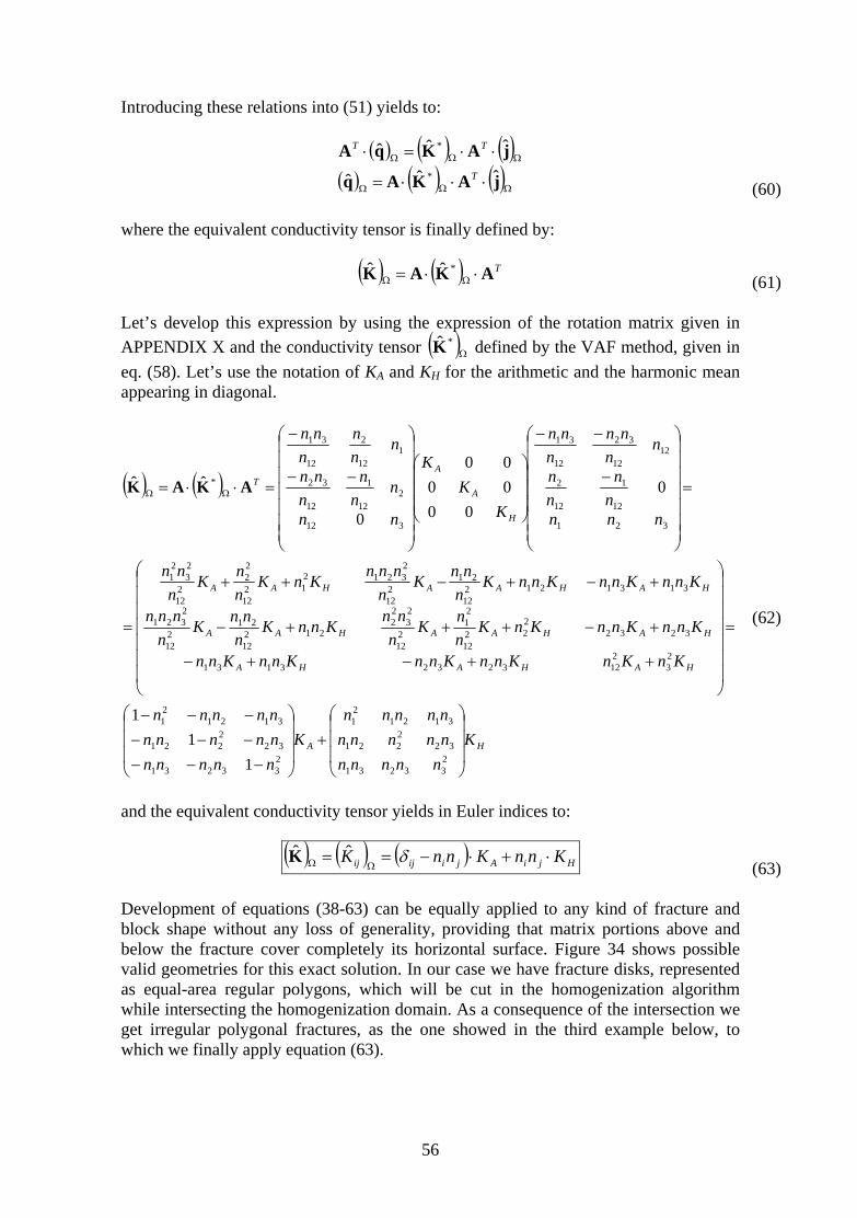
Introducing these relations into (51) yields to:

( ) ( ) ( )( ) ( ) ( )ΩΩΩ

ΩΩΩ

⋅⋅⋅=

⋅⋅=⋅

jAKAq

jAKqAˆˆˆ

ˆˆˆ*

*

T

TT

(60) where the equivalent conductivity tensor is finally defined by:

( ) ( ) TAKAK ⋅⋅= ΩΩ*ˆˆ

(61)

Let’s develop this expression by using the expression of the rotation matrix given in APPENDIX X and the conductivity tensor

( )Ω*K defined by the VAF method, given in

eq. (58). Let’s use the notation of KA and KH for the arithmetic and the harmonic mean ppearing in diagonal.

a

) ( )(

HA

nnnnnn

nnnnnn

⎟⎠

⎜⎝

⎟⎠

⎜⎝ −−− 2

33231

32221233231

32221

1 and the equivalent conductivity tensor yields in Euler indices to:

HAHAHA

AHAAHAA

HAHAAHAA

A

AT

Knnnnnnnnn

Knnnnnnnnn

KnKnKnnKnnKnnKnn

nKnnKnKnnK

nnnKnnK

nnnK

nnnn

KnnKnnKnnKnnnK

nnnnKnK

nnK

nnn

n

nn

nn

nnn

nn

KK

nnnn

nnn

nnn

⎟⎟⎞

⎜⎜⎛

+⎟⎟⎞⎛

−−−−−−

⎟⎟

⎟⎟⎟

⎠

⎞

⎜⎜⎜⎜⎜⎜⎜

⎝

⎛

++−+−

+−+++−

+−+−++

=

⎟

⎟⎟⎟⎟

⎠

⎞

⎜

⎜⎜⎜⎜

⎝

⎛

−

−−

⎟⎟⎞

⎜⎜⎛

⎟

⎟⎟⎟⎟

⎠

⎞

⎜

⎜⎜⎜⎜

⎝

⎛

−−

−

=⋅⋅= ΩΩ

23121

21

23121

21

23

21232323131

32222

12

21

212

23

22

21212

21212

2321

313121212

21212

23212

1212

22

212

23

21

3

12

1212

32

12

31

2132

112

2

12

31

*

11

00000

ˆˆ AKA

(62)

K

H nnnn

Knnnn

⎟⎟

⎜⎜⎟

⎠⎜⎝⎟

⎟⎜⎜

21

1212

312

1212 000

HKn =⎟⎟= 32

⎜⎜

( ) ( ) ( ) HjiAjiijij KnnKnnK ⋅+⋅−==

ΩΩ δK ˆˆ

Development of equations (38-63) can be equally applied to any kind of fr

(63)

acture and lock shape without any loss of generality, providing that matrix portions above and

exa tion

nal fractures, as the one showed in the third example below, to hich we finally apply equation (63).

bbelow the fracture cover completely its horizontal surface. Figure 34 shows possible valid geometries for this ct solu . In our case we have fracture disks, represented as equal-area regular polygons, which will be cut in the homogenization algorithm while intersecting the homogenization domain. As a consequence of the intersection we get irregular polygow

56

Figure 34: possible prismatic configurations for a valid fractured block fulfilling eq. (63).

Remark: it is important to note the result that appears when particularizing for the case of a 2D impermeable fractured medium with isotropic Poiseuille KF (i,j = 1,2; KM = 0; KF

|| =KF

|

):

( ) ( )

( ) ( )( ) ( )

( ) ( )( ) ( ) ( )jiijF

F

jiFjiij

FM

jiFMjiij

HjiAjiijij

nnK

K

nnKnn

KK

nnKKnn

KnnKnnK

−⋅⋅=

⎟⎟⎟⎟

⎠

⎞

⎜⎜⎜⎜

⎝

⎛

+−

⋅+⋅+⋅−⋅−

=

⎟⎟⎟⎟

⎠

⎞

⎜⎜⎜⎜

⎝

⎛

+−

⋅+⋅+⋅−⋅−=

=⋅+⋅−=

⊥

Ω

δϕϕϕ

ϕϕδ

ϕϕϕϕδ

δ

01

101

111

ˆ

|| (64)

which corresponds to the equivalent conductivity of [5] for a 2D fracture ‘F ’.

edium, fractures intersect with others in an irregular way. Taking at into account, the superposition of the individual fractured

section would also lead to matrix/fracture blocks intersecting with each other. To be

EVALUATION OF INDIVIDUAL FRACTURED BLOCK SIZE

In a fractured mth blocks of the previous

consistent from a mass conservation point of view, we choose the block size of each fractured block in an appropriate manner, such that the total volume of the fractured domain Ψ is preserved. Indeed, we set the block volume associated to the fracture ‘f’, denoted by fVΩ , to be proportional to the corresponding fracture surface in the following way:

ff VV ⋅= ΨΩ

mA∑ m A (65)

57

if the block is prismatic, the transversal dimension of the block b can then be identified

with the fraction ∑Ψ

m

mAV

ogenization dom

. Knowing that the specific surface of a fracture with respect

to the hom ain can be defined, neglecting the lateral faces of the

fracture, as Ψ

⋅=

VA f

f 2σ , we can also express the block height b in terms of this

parameter as follows:

∑

=

m

mbσ2 (66)

cal; its transverse thickness b depends on the fracturing density of the total volume Vψ. ecall that ψ is the homogenization domain.

s inside ψ, so that the hydro-mechanical parameters to calculate can be liable (see figure in [56] for inhomogeneous Poisson networks).

Lets denote by σ Ψ the sum of the specific surfaces of the fractures within the domain, .From this definition of the block volume, the volumetric fractions of

fracture, ϕ, and matrix, (1-ϕ), inside each prismatic block can be derived:

Equation (65) gives a local volume of each block. However, only the area of the block is loR Remark: the size of ψ should be chosen such that fracture density is relatively homogeneoure

∑m

mσ

( )22

Ψ

ΨΩ

Ω ⋅==

⋅⋅

==σ

σϕ

ff

f

ffF aa

bAaA

VV

(67)

5.3.2.2 Domain upscaling: superposition approach for discharge rates

. In the ischarge

previous section, we have c

The objective here is to homogenize up to a macro-scale domain

superposition approach, contributions of each fractured block to the global drate are summed up, given a known frozen head gradient J. In the

omputed the block-scale equivalent hydraulic coefficient, which describes the hydraulic response of the block to any given global head gradient. Now, to upscale we have to add up contributions of each individual fractured block of some measurable quantity, such as the discharge rate. First, let’s calculate the discharge rate Q flowing out from an individual block from the flux density q obtained in the previous section, that is:

( ) ( )( )Ω

Γ Ω

Ω ⋅=⋅

=∫

qq

Q ˆ2

ˆˆ

FLOWAds

F (68)

ds is the surface differential element and AFLOWthe projection of the outgoing-flux surface of the block in the normal plane to each component of the flux density q. Note that q is not a net flux but a flow-through flux.

where is a diagonal matrix that express

58

Figure 35 shows an example of two-component flow through an inclined block and the corresponding out x surfaces for each component.

going-flu

b

n

⎟⎟

⎞

⎜

⎛=

1

0J

J⎟

⎠⎜

⎜

⎝ 3J

3u5n

5n

1u2n

1u

l1l2

l4

l3

2u

3u

1u 4n

3u

AFLOW matrix: projection Figure 35: Example of the of the outgoing-flux surface of the block in the normal plane to each component direction of the flux.

The outflow surface AFLOW is computed as follows for a prismatic block, whatever the shape of the polygonal fracture is:

( )∑<

⋅= fff nAA (69)

2πθki

kkikFLOW

where, for fractured block ‘f ’, Ak = A f for the base faces and Ak = lk ·b for the lateral ces of the prismatic block ; θki is the angle between unitary vectors and . Note

integral over the teral perimeter of the block. Indeed, due to symmetry of a prismatic block face

project

kn iufathat for other fracture shapes, the sum for the lateral faces becomes an la

ions into negative or positive sense for a give direction, the matrix fFLOWA can be

initially computed independently of the direction of the flux (more on this in the remark further below). The superposition can now be carried out by adding up the individual contributions of each block to the global discharge rate: ∑= mQQ

m(70)

Substituting the results obtained in the previous equations into (70), the global discharge

te yields to: ra

( ) ( ) ( )( ) ( )∑ ∑ ⋅⎥⎥⎦⎢

⎢⎣

⎟⎟⎠

⎜⎜⎝

+⋅++⋅−⋅−⋅⎥⎥⎦⎢

⎢⎣

⋅= ⊥

<m

jFM

mj

miFM

mmj

miij

kki

mki J

KKnnKKnnnAQ

ki

||1

2

ϕϕδπθ

(71)

⎤⎡ ⎞⎛ −⋅⎥

⎤⎢⎡ −mm

mm1

1 ϕϕ

59

To convert into hydraulic conductivity we have to divide by the total outflow surface on each direction. The equivalent hydraulic conductivity finally yields to:

( ) ( ) ( )( ) ( )

( )∑ ∑

∑ ∑

<

−

⊥

<

⋅

⎥⎥⎦

⎤

⎢⎢⎣

⎡⎟⎟⎠

⎞⎜⎜⎝

⎛+

−⋅+⋅+⋅−⋅−⋅

⎥⎥⎥

⎦

⎤

⎢⎢⎢

⎣

⎡⋅

=

f k

fki

fk

f F

f

M

ffj

fiF

fM

ffj

fiij

k

fki

fk

ij

ki

ki

nA

KKnnKKnnnA

K

2

2

1|| 11

π

π

θ

θ

ϕϕϕϕδ

(72)

Remark: In expression (72), the equivalent hydraulic conductivity seems to depend indirectly on the direction of the global hydraulic gradient, by terms of the outgoing-flux area AFLOW defined in equation (69). However, if flow goes in the contrary direction, it is easy to show that the sum of the area projections in the normal plane is exactly the same as computed for the other sense. Therefore, the equivalent hydraulic conductivity tensor, or more precisely, the corresponding equivalent intrinsic permeability, def .e., is really an intrinsic property arge rates by multiplying for flux direction appears.

ARTICULAR CASES

t general expression of the equivalent hydraulic onductivity for the domain defined in Figure 32. Let’s see some particular cases to heck the behaviour of this formula to approximate frac

ples, we distinguish between different configurations of the fractured

1

ses coincides with the domain block, and b=l3. Also, the equivalent

an appreciate the effect of the flow direction: me for the three cases,

discharge rates vary according to the flow d - Inclined single fracture (Figure 36d): corresponds to a fractured medium in

ined here is independent of the flow direction, i of the medium. Afterwards, when computing the dischthe hydraulic gradient, then the dependence on the

P

Equation (72) is the moscc tured media.

In the first examnetwork. The domain is a cubic block of VΨ=l1x l2x l3 crossed by fractures completely. Fractures are identified by the cardinals F=1,2, etc; fracture area by A , A2, etc. Both cases with KM≠0 and KM=0 are showed:

- Parallel single fracture (Figures 36a, 36b, and 36c): correspond to a fractured medium with only one fracture, parallel to the domain faces. This is exactly the same configuration as the individual fractured block used above for the exact low-order flow computation. Therefore, the corresponding individual fractured block for these caconductivity tensor is the same as the exact conductivity tensor of the low-order computation. However, here we calthough the equivalent hydraulic conductivity is the sa

irection on each case.

which the only existing fracture is inclined. Thus, the individual fractured block for the upscaling will also be inclined, as showed in the figure, and

23

2131 llllAVb f +⋅== Ψ .

60

- Simplest cartesian network (Figures 36e): corresponds to a ‘3D cross-shaped’ medium , with three fractures perpendicular to each other and intersecting in the center of the domain. In this case, ( ) 11

31

21

1−−−−

Ψ ++== lllAVb f .

We can also consider other type of particular cases related to the nature of the fracture itself. Equation (72) corresponds to the case of a permeable medium with a fault-likfracture, that is, a fracture filled with porous material surrounded by the porous matrixIf the filling of the fracture is isotropic, then . However, this expression can lso be particularized to other cases according to the nature of the fracture: for example,

e .

||FF KK =⊥

aif the fracture is ‘opened’, then ∞=⊥

FK and .|| PoisFF KK = , where .Pois

FK is the Poiseuille

conductivity given by the expression: ( )γ⋅

⋅=

12

2.

fPoisF

agK . Some particular cases may be:

- Impermeable fault-like fractured medium ( 0=MK ):

( ) ( )[ ]

( )∑ ∑<

⋅=

f k

fki

fk

ij

ki

nAK

2πθ

-

∑ ∑<

⋅⋅−⋅⎥⎥⎥

⎦

⎤

⎢⎢⎢

⎣

⎡⋅

fF

ffj

fiij

k

fki

fk

ki

KnnnA

2

||

πθ

ϕδ

(73)

Permeable fractured medium ( .||; PoisFFF KKK =∞=⊥ ):

( ) ( ) ( )( )

( )( )∑ ∑

<

<

⋅

⎦⎣⎥⎦⎢⎣=

f k

fki

fk

f k

ij

ki

ki

nAK

2

2

π

π

θ

θ

- Impermeable fractured medium

∑ ∑ ⎢⎡

+⋅+⋅−⋅−⋅⎥⎤

⎢⎡

⋅ Poisffffff nKKnnnA 1 .ϕϕδ ⎥⎤

−⋅⎥⎢ f

Mfj

fiFMjiijkik

Kn1 ϕ

(74)

( .||;;0 PoisFFFM KKKK =∞== ⊥ ):

( ) ( )[ ]

( )∑ ∑

∑ ∑

<

<

⋅

⋅⋅−⋅⎥⎥⎥

⎦

⎤

⎢⎢⎢

⎣

⎡⋅

=

f k

fki

fk

f

PoisF

ffj

fiij

k

fki

fk

ij

ki

ki

nA

KnnnA

K

2

2

.

π

π

θ

θ

ϕδ

rk: Developing, again, the case of a 2D impermeable fractured medium (BMT3 ields to:

(75)

Remacase)

y

( ) ( )∑∑ ⋅−⋅⋅⋅

⋅=⋅⎥⎦

⎤⎢⎣

⎡⋅

⋅⋅

⋅⋅−⋅=

Ψ Fjjiij

F

F

Fjjiiji JnngaJag

AaLnnaQ δ

σφ

γγδ 2

32

1212

e expression obtained in [5].

(76)

which corresponds exactly with th

61

62

FRACTURED DOMAIN KM ≠ 0 KM = 0

=1

a.

F

1n

=J

AFLOW

KAQQQ

H⋅==

⎟⎟⎟

⎠

⎞

⎜⎜⎜

⎝

⎛

3

00

J

3J⋅13

2

1

00=

ij

KK

KK

0000

⎟⎟⎟

⎠

⎞

⎜⎜⎜

⎝

⎛=

H

A

A

00

3

2

1

==

000=

QQQ

=ijK⎟⎟⎟

⎠

⎞

⎜⎜⎜

⎝

⎛

00000

0||

||

F

F

KK 0

=1

F

1n ⎜⎜⎜

⎝

⎛=J

AFL

b.

⎟⎟⎟

⎠

⎞

00

1J

OW

00

3

2

121

==

⋅⋅⋅=

QQ

blQ ij

KK

KK

00000

||1

==

⋅⋅=

QQ

Kl F

0000

JKA

⎟⎟⎟

⎠

⎞

⎜⎜⎜

⎝

⎛=

H

A

A

0

112 ⋅ Ja =ijK

00

3

2

Q

⎟⎟⎟

⎠

⎞

⎜⎜⎜

⎝

⎛

00

0||

||

F

F

KK

⎟⎟⎟

⎠

⎞

2

1J

⎜⎜⎜

⎝

⎛=

3JJJ

AFLO

1n

F=1

W c.

212

121

JKAJKblQJKblQ

H

A

A

⋅⋅=⋅⋅⋅=

313Q

⋅⋅⋅=

⎞

⎜⎜⎜

⎝

⎛=

H

A

A

ij

KK

KK

00000

2

1

⋅=

⋅=

lQ

l

F

00000||

FK

⎟⎠

⎟⎟

0

3

2||

21

1||

12

=⋅⋅

⋅⋅

QJKa

JKa F

=ijK0

Q

⎟⎟⎟

⎠

⎞

⎜⎜⎜

⎝

⎛

0

0||FK

Fig 36: Results of the global discharge rate (eq. 68) and the equivalent aulic conductiv eq cular ity ( . 72) for some partihydrure cases.

F=1

n

⎟⎟⎟

⎠

⎞

⎜⎜⎜

⎝

⎛=

3

2

1

JJJ

J

AFLOW, 1

AFLOW, 2

AFLOW, 3

b

d.

⎥⎦

⎤⎢⎣

⎡⋅⎟

⎞ JKA

⎠⎜⎝⎛ −

+⋅⎟⎠⎞

⎜⎝⎛ +

⋅⎟⎟

⎠

⎞

⎜⎜

⎝

⎛

++⋅⋅=

⋅⋅+⋅=

⎥⎦

⎤⎢⎣

⎡⋅⎟

⎠⎞

⎜⎝⎛ −

+⋅⎟⎠⎞

⎜⎝⎛ +

⋅⎟⎟

⎠

⎞

⎜⎜

⎝

⎛

++

+⋅⋅=

1323

21

112

32

1

323

22

32

12

3123

21

123

21

121

22

22

KKK

ll

l

ll

llbQ

JKllbQ

JKKJKK

lA

ll

llbQ

HAH

A

AHAH

⋅+ JA

⋅ 3l

l

⎟⎟⎟⎟⎟⎟

⎠

⎞

⎜⎜⎜⎜⎜⎜

⎝

⎛

⎟⎠⎞

⎜⎝⎛ +

⎟⎠⎞

⎜⎝⎛ −

⎟⎠⎞

⎜⎝⎛ −

⎟⎠⎞

⎜⎝⎛ +

=

20

2

002

02

AHAH

A

AHAH

ij

KKKKK

KKKK

K

( )

( )1311

3223

21

32 ll

F

+⋅=

1

||

2||2

32

112

3131

1223

21

12

JJb

lAllKaQ

JKllaQ

JJb

lAllll

aQ

F

−⋅⎟⎠⎞

⎜⎝⎛ ⋅

+⋅⋅⋅

⋅⋅+=

−⋅⎟⎠⎞

⎜⎝⎛ ⋅

+⋅+⋅

=

||1 KF ⋅⋅

⋅

⎟⎟⎟⎟⎟

⎠

⎞

⎜⎜⎜⎜⎜⎛

−

−

=

20

2

002

02

||||

||

||||

FF

F

FF

ij

KKK

KK

K

⎝

b

F=1

1n

⎟⎟⎟

⎠

⎞

⎜⎜⎜

⎝

⎛=

3

2

1

JJJ

J AFLOW, 1

2n

3nF=2

F=3 AFLOW, 2

AFLOW, 3

e.

( )[ ]( )[ ]( )[ ] 32133

23122

321

JKbllKAQJKbllKAQJKbllQ

AH

AH

AH

⋅⋅⋅++⋅=⋅⋅⋅++⋅=⋅⋅ 11 KA ⋅++⋅=

( )( )( )( )( )( )

( )jiK

bllAKbllKA

bllAKbllKA ⎟

⎜⎜⎜⎜⎛

= 2

bllKbllKA

K

ij

AH

AH

A

ii

≠=

⎟⎟⎟⎟

⎟⎟⎟

⎠

⎞

⎜⎜⎜

⎜⎜⎜

⎝

⎛

⎟⎟⎠

⎞⎜⎜⎝

⎛⋅++

⋅⋅++⋅

⎟⎟⎠

⎞

⎝ ⋅++⋅⋅++⋅

⎟⎟⎠

⎞⎜⎜⎝

⎛⋅++

⋅⋅++⋅

0213

213

312

31

321

321

AH

( )( )( )( )( )( ) 3

||

321

33213

2||

321

22312

1||

321

11321 A

Q ⎢⎣

=

JKAAAAalQ

JKAAAAallQ

JKAAAall

F

F

F

⋅⎥⎦

⎤⎢⎣

⎡⋅

+⋅⋅+

=

⋅⎥⎦

⎤⎢⎣

⎡⋅

++⋅⋅+

=

⋅⎥⎦

⎤⎡⋅

++⋅⋅+

l+

( )( )( ) ( )( )( )( ) ( )( )( )( ) ( )

( )jiK

AAAbllAKAall

AAAbllAKAall

AAAbllA⎜⎜⎜ ⎟

⎠⎜⎜⎝ +1

KAall

K

F

F

F

ii

⎟⎟⎟⎟⎟⎟⎟⎟

⎠

⎞

⎜⎜⎜⎜⎜

⎝

⎛

⎟⎟⎠

⎞⎜⎜⎝

⎛++⋅⋅++

⋅⋅⋅+

⎟⎟⎠

⎞⎜⎜⎝

⎛++⋅⋅++

⋅⋅⋅+

⎟⎞⎛

++⋅⋅+⋅⋅⋅+

=

321213

||3321

321312

||2231

32132

||1132

ij ≠= 0

Figure 36(cont.): Results of the global discharge rate (eq. 68) and the equivalent hydraulic conductivity (eq. 72) for some particular cases.

63

64

5.3.3 Mechanic and hydro-mechanic equivalent coefficients

A strain-based superposition approach was developed in [71] to obtain equivalent hydromechanical laws for an elastic rock containing many fractures. The individual fractures or fractures were assumed to behave elastically or quasilinearlyunder compression and shear [71], and to satisfy Terzaghi's ‘effective stress’ approximation [86].

Our implementation assumes linear elastic laws with constant coefficients. The mean strain, due to the imposed global stress tensor σij, is calculated by linear superposition of the local displacements occurring throughout the intact rock matrix and the discrete fractures, keeping the global stress constant. This leads to linear hydro-mechanical lawscoupling solid stress and fluid pressure to solid strain and fluid strain (or fluid production), similar to the poro-elastic laws developed earlier by Biot [13][14]. The homogenized hydromechanical relations developed by [71] are summarized below. These relations were obtained by applying a superposition principle to the displacements (and strains) occurring, respectively, in the fractures and in the rock matrix between the fractures, for a given stress field (assumed the samethroughout the rock mass), similarly to the approach followed for the hydraulic homogenization. Oda’s relations are expressed in terms of probability distribution integrals, and BMT3 work adapted them to discrete sums of empirical distributions over the whole set of fractures. These are the expressions we have used for our work. The mean (homogenized) fractured rock strain tensor is related to total (global) stressand to fluid pressure by the following relation (we use overbars to designate the averages or homogenized quantities coming from Oda's work): pBT ijklijklij += σε (77) with: ijklijklijkl CMT +=

ijklT = Total homogenized compliance tensor

ijklM = Compliance tensor of the isotropic rock matrix

ijklC = Compliance tensor due solely to fractures

ijB = Homogenized strain-pressure coupling coefficient (‘barred’ Biot coefficient)

The 'matrix' compliance - characterizing the perfectly elastic, isotropic, intact rock matrix - is given by the 4th rank tensor:

( ) klijjkiljlikijkl EEM δδνδδδδν

−++

=211

where E is Young's modulus (pressure units) and ν is the Poisson ratio (dimensionless).

'global'

(78)

The 'fractures' compliance - characterizing the specific contribution of the fracture stem to the total compliance of the fractured rock mass - is given by the 4th rank

tensor:sy

ijklijklijkl Gg

Fgh

C 111+⎟⎟

⎠

⎞⎜⎜⎝

⎛−= (

79)

re, no onnectivity issues are needed in this approach [55][71].

In this equation, Fijkl and Gijkl are geometric tensors independent of elastic properties of the matrix or fractures, and related only to fracture density and to the distributions of fracture orientations, lengths, and apertures. The precise expressions of these tensorial parameters will be given below, after [71]. It should be emphasized right away that these so-called 'geometric' tensors do not depend on any other configuration parameter of the fracture network; in particular, they are not explicitly related to the spatial locations of individual fractures, of fracture intersections, etc. Therefoc The parameters ( , )h g are directly related to the mean elastic properties of the fractures, namely, their shear stiffness modulus (Ks) and their normal stiffness modulus (Kn). Here we assume that the individual fractures have constant shear stiffness and normal stiffness moduli, Ks and Kn, and we use an approximation of Oda's expressions, which can be expressed as follows:

lKh n≈ (80)

lKg s≈ where l is the mean length of fractures over the homogenization domain. In our case,

r planar circular fractures, l is the mean diameter of fractures, R2 .fo

s original formulation, the fracture stiffness coefficients were taken to be linear nctions of the ambient effective stress (projected on the fracture's normal vector). da's model leads to increasing (shear and normal) stiffnesses for a fracture that is

decreasing stiffness for a fracture th tensile normal stresses. Future developmen ude dependencies as the ones used i The so-cal

Geom F

In Oda'fuObeing closed by compressive normal stresses, and also,

at is being opened or re-opened byts of the hydro-mechanical upscaling could incl

n [71].

led 'geometric tensors', Fijkl and Gijkl, are given below:

etrical Tensors ijkl and Fij (Empirical discrete sums instead of Oda’s integral expressions):

( ) ( ) ( ) ( )

( ) ( )∑

∑

=

=

==

=

N

ffjfiffijkkij

N1f

flfkfjfiffijkl

nnFF

nnnnF1

21

2

σ

σ

(81)

1

65

Geometrical Tensor Gijkl (Derived from Fijkl):

( )ikjljkililjkjlikijkl FFFFG δδδδ +++=41 (82)

ations, represents the length of fracture f (fracture diam

In these equ eter), nf f the unit vector normal to the fracture f, and σ the specific area of fracture f with respect to the fhomogenization domain, which was defined earlier. Finally, we now give an explicit expression for the remaining tensorial coefficient, B , that couples strain to fluid pressure in Oda's strain equation (77). According to [71], this 2nd rank tensor is related to the 4th rank fracture compliance tensor C , as follows: ijkkij CB = (83) A more explicit result can be obtained after calculating the contracted fracture compliance tensor (on the right-hand side). To obtain the final result, we note first that the contracted tensor Gijkl yields Fij, based on equation (2-15). Using this identity, it can then be seen from equation (2-11) that the contracted tensor ijklC yields hFij . In short, the final result is:

ijij Fh

B 1= (84)

On the other hand, Oda's relations lead to the pressure/strain constitutive law of fluid production given in eq. (5), neglecting here the thermal term. This relation can be restated as follows:

( )ξ−−= klkl eBGP ( which is exactly of the same form as the corresponding anisotropic Biot equation. This law involves the scalar Biot modulus G and the 2nd rank tensorial coefficient of Biot B

85)

ij. For a fractured rock mass, G is given by any of the following formulas (they are all equivalent):

( ) ( ) 1−

ijijij

( ) 1−−= BBT δ

1−

−=

−=

ijijklijkl

klijklijij BTB

BBG

δ

δ

(86)

while Bij and the associated (barred) quantity are given by:

hFBBTB ijijklijklij == ; (87) The full derivation of these formulas for the Biot coefficients can be found in [5].

66

5.3.4. Implementation and results of the upscaling

.3.4.1 REV study and moving average 5

The volume of the homogenisation subdomains has been determined by means m

omogenization formula (72).

bdomain. Figure 37 shows the result of this calculation, where the block size of 20 eters has been set to be the REV of the fracture

ogenization blocks containing any portion of these fractures will roduce a somehow smoothed profile of hydraulic conductivity in the transversal irection. This effect has coherence with the na

faulty-like damaged zone around them that decreases the conductivity gradually towards e rock matrix.

Figure 37: REV determination for Kij in the simulated fractured medium.

of the Representative Elementary Volume (REV). It is defined as the minimu volume where computed parameters can be considered to be ergodic or statistically stationary. In our case, the minimum block volume has been estimated by with respect to the quivalent hydraulic conductivity resulting from the he

To determine the REV of our fractured medium, we have computed the mean square root of the diagonal components of the hydraulic conductivity tensor (square root of the sum of squares) for increasing homogenisation sizes in different points of the sum d medium. It is important to note that the 17 fixed fractures have been taken out from the REV study, because they have been created with different statistics than the rest of the fractured medium (uniform distributions instead of power law for the fracture size pdf). Afterwards, the big fractures will be included in the homogenisation with the chosen REV, so that these important features are taken into account for the hydraulic model.

oing so, the homDpd ture, as the big fractures use to have a

th

P=(0,0,0) P=(0,-65,0) P=(0,65,0) P=(0,30,0) P=(0,-30,0) P=(-15,0,0) P=(15,0,0)

67

Once the optimized fractured medium has been obtained and the up-scaling formula has een defined, the computation of the equivalent parameters can be achieved. This has

indow with a window size equal to the REV of e discrete jump of the window has been set to

0m, i

rnal

bbeen done through a moving average whe fractured medium, that is, 20m. Tht

1 n order to be approximately of the same order of magnitude than the finite element mesh mean size. The resulting moving average will lead to matrices of equivalent coefficients of size 5x18x5 for each of the homogenized parameters. Implementation of the upscaling routine has been done in MATLAB®. Due to the normous size of the fracture data file, and to memory limitations, an intee

subroutine to compute intersections by subsets of the fractured data has been developed. The algorithms followed to compute the up-scaled coefficients are presented in Figures 38 and 39.

INITIALIZE variables:

k T B G ϕ f α ij, ijkl, ij, , , Fijkl, Fij, Gijkl, C’ijkl, M’ijkl, T’ijkl

For 1: Subdomain

For 1: Nsubset: Nfractures

Compute Fracture Intersections (*)

Load fracture data

Add intersecting fractures to subdomain intersections array

Compute equivalent upscaled coefficients:

kij, Tijkl, Bij, G, ϕ f, α

SAVE computed variables: kij, Tijkl, Bij, G, ϕ f, α

Fijkl, Fij, Gijkl, C’ijkl, M’ijkl, T’ijkl

Figure 38: Algorithm of the upscaling process. The algorithm of fracture intersections with the homogenization subdoma(*) in is

showed in the next figure.

68

LOAD fracture data matrix:

(node coordinates of regular polygon approximating circular fractures)

Exclude fractures outside the subdomain

Compute intersection of fractures bigger than the subdomain

Compute intersection of the rest of fractures

SAVE fracture intersection matrix

Compute intersections of lines with subdomain faces

Choose fracture center or interior point close to it

Build lines parallel to the axes passing through the

interior point

Compute intersections of lines with

subdomain edges

Compute intersections of fracture polygon edges

with the subdomain faces

Build lines in the fracture plane passing through the face intersection points.

Build intersecting irregular polygon coordinates matrix

Figure 39: Algorithm of fractured medium intersections with the homogenization subdomain.

5.3.4.2 One-block homogenization A one-block homogenization has been performed. Equivalent coefficients for the whole domain have been computed. Results show a quasi isotropic equivalent medium in hydraulic conductivity and a quasi-orthotropic medium for the mechanical stiffness tensor. The equivalent intrinsic permeability of the fractured medium is:

(88)

with the following eigenvalues and eigenvectors of the principal axes directions:

03157.02163.07708.05495.04242.06269.07735.0

;10107.1000142.1000055.1

218 vmkij with

Figu sic permeability.

21810099.1013.0009.0015.0112.1034.0017.0043.0092.1

mkij−⋅

⎟⎟⎟

⎠

⎞

⎜⎜⎜

⎝

⎛

−

−=

⎟⎟⎟

⎠

⎞

⎜⎜⎜

⎝

⎛

−

−−=⋅

⎟⎟⎟

⎠

⎞

⎜⎜⎜

⎝

⎛= −∗

8794.01133.

re 40 shows four different views of the ellipsoid of equivalent intrin

69

Figure 40: Equivalent intrinsic permeability ellipsoid for the one-block homogenization of the fractured medium.

The equivalent mechanic stiffness of the fr red medium, in reduced matricial form, is:

9100514.01679.03643.031589.00146.02142.04194.25982.34461.21338.00212.02865.24461.21096.3

⋅⎟⎟⎟⎟⎞

⎜

⎜⎜⎛

−−−−

=

e approximation of the stiffness tensor to orthotropic medium would be:

0004194.25982.34461.20002865.24461.21096.3

⎟⎟⎟

⎟⎟⎟

⎠

⎞

⎜⎜⎜

⎜⎜⎜

⎝

⎛

he first quarter of the matrix (we denote it Tij) can be represented as the permeability,

actu

0167.0−

393.54194.22865.2⎜T Paijkl

8336.00660.00161.00514.01589.01338.00660.05725.00777.01679.00146.00212.00161.00777.08816.03543.02142.00167.0

⎟⎟⎟⎟

⎠⎜⎜⎜⎜

⎝ −−−−−−−−−−−

Th

PaT l910

0003933.54194.22865.2⋅

⎟⎟

⎜⎜= ijk

8336.00000005725.00000008816.0000

Tby computing its principal axes (eigenvectors) and principal components (eigenvalues) (see Figure 41):

70

⎟⎟⎟

⎠

⎞

⎜⎜⎜

⎝

⎛

−−

−=⋅

⎟⎟⎟

⎠

⎞

⎜⎜⎜

⎝

⎛=∗

6846.07283.00318.05363.05328.06546.04937.04310.07553.0

;109378.80002700.20008933.0

9 vPaTij

There is one order of magnitude of difference between the minimum and the maximum stiffness principal components. The direction of anisotropy could be influenced by the big fractures orientation.

Figure 41: Equivalent reduced stiffness tensor ellipsoid for the one-block

homogenization of the fractured medium. The Biot coefficient for the homogenized medium is:

⎟

⎠

⎞

⎜

⎜

⎝

⎛

−

−−

9271.00163.00022.0

0022.00186.09401.0

with the following principal components and directions:

lipsoid.

⎟⎟⎜−= 0163.09411.00186.0ijB

⎟⎟⎟

⎠

⎞

⎜⎜⎜

⎝

⎛−

−−=

⎟⎟⎟

⎠

⎞

⎜⎜⎜

⎝

⎛=∗

3525.06553.06681.07255.02596.06374.05911.07094.03839.0

;9642.00009313.00009129.0

vBij

These values of the Biot coefficient imply that there exist a high coupling between hydraulics and mechanics, and hydraulic pressure is transmitted to the matrix in form of stresses in more than a 90% for all directions, almost isotropic. Figure 42 shows the orresponding elc

71

Figure 42: Equivalent Biot coefficient ellipsoid for the one-block homogenization of

the fractured medium. The homogenized Biot modulus G is:

he rest of intermediate 2nd and 4th rank tensors of the one-block homogenization can b ound

.3.4.3 Moving average homogenization

PaG 10101877.4 ⋅=

Tf

ein the APPENDIX XI.

5

ogenization yield to a 5x18x5 parameter values spatially located within a partition of the domain. Main features

of the fractured medium can be appreciated in the heterogeneity of the parameters along the domain.

tridimensional view of the intrinsic permeability ellipsoids is displayed in Figure 43a. plane for the five X-layers of

rientations mostly NNW-SSE amily 2) influences the heterogeneous distribution of permeability. Thus, fractures

crossing the FEBEX drift at the test zone provide a preferential NNW-SSE flowpath. In the rest of the domain, the permeability heterogeneities are less remarkable, although clear differences among permeability ellipsoids in contiguous subdomains can still be ppreciated. Big fractures also have an effect in the equivalent stiffness tensor (Figure

32 is also represented in Figures 47a-e as spheres.

The results of the moving average process of hom

set of

AFigures 44a-e show projections of the ellipsoids in the YZomogenization. The presence of big fractures with oh

(f

a43b and Figures 45a-e), which gets smaller (softer medium) as the fracture density increases. This will imply a higher deformation in the FEBEX area than in the rest of the domain. However, Biot coefficient (Figure 43c and Figures 46a-e) and Biot modulus are much more homogeneous within the domain partitions. The volumetric fracture

ensity ρ (scalar values)d

72

a.

b.

c.

Figure 43: Hydraulic and hydro-mechanic equivalent coefficients for the moving average homogenization. a. Equivalent intrinsic permeability kij; b. Equivalent stiffness tensor Tijkl (only Tij with i,j=1,2,3); c. Equivalent Biot coefficient Bij.

73

a.

b.

c.

d.

e. igure 44: Equivalent intrinsic permeability kF ij for the five X-layers of the moving

average: (kij)min=1.09·10-18 m2, (kij)max=6.91·10-18 m2.

74

a.

b.

c.

d.

e. Figure 45: Equivalent stiffness tensor Tijkl (only Tij with i,j=1,2,3) for the five X-

the moving average: (Tlayers of mi x ·1010 Pa. ij) n=8.18·108 Pa, (Tij)ma =3.21

75

a.

b.

c.

d.

e. Figure 46: Equivalent Biot coefficient Bij for the five X-layers of the moving

average: (Bij)min=0.73 , (Bij)max=1.

76

a.

b.

c.

d.

e.Figure 47: Equivalent volumetric fracture density for the five X-layers of the moving

average: (ϕf)min=1.54·10-5 , (ϕf)max=2.53·10-5.

77

6 IMPLEMENTATION AND RESULTS OF THE THM MODEL 6.1 Domain and problem definition The domain is a block with the Geographic North oriented towards –X. The dimensions of the block are 70m x 100m x 70m, with the origin of coordinates in the center of block. There are three connected drifts: the Main tunnel, the Laboratory tunnel and the FEBEX drift, the last one being centered in the origin of coordinates. In the test zone of the FEBEX drift there exist a heating process defined here by a temperature gradient from 100ºC at r=0m to 35ºC at r=1.14m, being r the radial direction in the FEBEX drift. Figure 1 shows the domain considered, along with the nomenclature for the boundaries.

N

FEBEX test zone

FEBEX drift Laboratory tunnel Main tunnel

Figure 48: Domain of the THM model and boundaries nomenclature. The problem has been simulated in three different stages:

- Hydro-lithostatic equilibrium of the rock mass: at this stage, there is no drift and a fully saturated 365m rock mass is assumed to be lying over the upper boundary of the domain. Both the hydrostatic and the lithostatic loads have been imposed gradually for the time-dependent analysis. The load profiles used are polynomial functions and are described further below. Relative fluid pressure is computed in all the models (P-Patm).

- Drifts excavation simulation: the HM response of the fractured rock is

analyzed during the excavation of the drifts, which has been modeled by gradually decreasing both the normal stresses and the fluid pressure in the boundaries of the excavated tunnels. The same kind of polynomial functions of the previous stage has been used for the decreasing profiles. Real hydraulic conditions existing in the Grimsel Test Site have been used this time.

79

- Heating experiment simulation: at this stage, the full THM model is used. A 3-year heating process has been simulated around the FEBEX test zone (last 17 m of the FEBEX drift). Heat load profile is determined by the FEBEX

ions. Two possible cases have been considered: the test zone is filled with bentonite [79][92][93] and the access drifts are not filled with any material; the test zone is filled with bentonite and the access

“In-situ” experiment condit

drifts are filled with some material similar to the surrounding rock. Only results corresponding to the first case are presented here.

Three different HM conditions of the rock have been compared in the analyses (the thermal conditions are in all the cases isotropic and homogeneous):

• HM-isotropic homogeneous material: with simplified values coming from the 1x1x1 homogenisation of the fractured rock domain.

• H-anisotropic and M-non-orthotropic homogeneous material: with the full

set of values of the 1x1x1 homogenisation of the fractured rock domain. • H-anisotropic and M-non-orthotropic heterogeneous material: with the

5x18x5 homogenisation of the fractured rock domain. The thermal transient is imposed and consists in a 3-year heating according to the FEBEX insitu experiment specifications. The thermal load is gradual, following the temperature profile of the experimental measurements. Two different loading functions have been tested (Figures 51a and 51b). The first one is an exponential function (Figure 49a), but it leads to convergence problems in the coupling with hydraulics. Thus, a polynomial function (Figure 49b) with zero derivative in t=0 has been used for the TH and THM models. At the maximum temperature point, the functions are defined as:

- Exponential function:

⎟⎠

⎜⎝

⎞⎛ −⋅=−

01100 tt

eT

- Polynomial function:

⎪⎩ > 0100 ttif

s 5·10

⎪⎨

⎥⎢ ⎟⎠⎞⎜

⎝⎛⋅+⎟

⎠⎞⎜

⎝⎛⋅−⋅

= 0032100 t

tt

tT

⎧≤

⎦

⎤

⎣

⎡0

23

ttif

Where t0 iloading tra The hidro hydrostatic and lithostatic stabilisation of the rock mass due to the 365-m rock weight existing over the domain (FEBE dboth hydrahas to be reflected inloading timeach of thloadings is the same as the polynomial function used for the thermal loading.

6 s = 57.87 days, approximately equal to the two month of the heat nsient of the FEBEX experiment to reach the 100ºC.

-mechanical transient has consisted in the

X rift is ~400m deep). A gradual loading has been used, as stated before, in ulic and mechanic models to assure convergence. However, the loading rate sufficiently fast so that the coupled hidro-mechanical processes can be the results without the influence of the loading conditions. Therefore, the e has to be at least 10 times smaller than the characteristic diffusion time for e processes. The function shape used for both hydraulic and mechanic

80

a. b.

Fig

A quick a the characteristic time for the hydraulic process and for the coupled hydromechanic process. The ori a

ure 49: Two heating profiles for the experiment simulations: a. Exponential function; b. Polynomial function.

nalysis of the hydraulic equation can yield to the determination of

gin l hydraulic equation of our system is:

⎥⎥⎦⎢

⎢⎣

⎟⎟⎠

⎞⎜⎜⎝

⎛

∂∂

+∂∂

⋅−∂∂

−=∂∂

+∂∂

+⎥⎥⎦⎢

⎢⎣

⎟⎟⎠

⎞⎜⎜⎝

⎛

∂

∂+

∂∂

∂∂

jw

jw

ij

iTweq

i

j

j

iij x

zgxPk

xtT

tP

Gxu

xu

tB ρ

µβθ1

21

Let us now consider only the terms in fluid pressure and constant values of the parameters for all the subdomain (1-block homogenization):

⎤⎡⎤⎡

jiw

ij PkP ∂∂∂1xx ∂∂

⋅= tG ∂ µ

We can e

th n write:

w

ijH

jiH

kGR

xP

xR

tP

µ⋅

=∂∂

∂∂

⋅=∂∂ with

here RH can be seen as a ‘characteristic diffusion rate’ for hydraulics.

block homogenization, H yields to:

w Considering the values of the parameters corresponding to the 1-R

046.0101

101.1101877.46

1810

=⋅

⋅⋅⋅= −

−

HR m2/s

and dividing some characteristic length of the domain, in our case L=70m, by the hydraulic rate RH, we get the characteristic time of the hydraulic process:

h29s1006.1046.0

70 522

=⋅===H RLt

H

81

To illustrate this concept, we plot the hydraulic pressure in two points at the top and bottom boundaries, for two different loading time scales. In the first case, the hydraulic loading time (t0=5e7s) is faster than the characteristic time of hydraulics, and the loading process at the bottom boundary (Figure 49b) is mainly due to the diffusion of the pressure introduced at the top boundary (Figure 49a). In the second case, the hydraulic loading time (t0=1e10s) is slower than the characteristic time, and loading process at the bottom (Figure 49d) reproduces the loading at the top (Figure 49c). We have taken the same t0 than in the thermal transient, i.e., t0=5e6s, as loading time scale for the hydraulic problem.

ble 2 resumes the numerical experimen p ned for the model. Both the final steady te analysis and the time dependent analysis have been carried out for each case:

Ta tsa

lanst

b.a.

Figure 50: Comparison between the effects of a hydraulic load at the top boundary in the bottom boundary for two different loading times.

Table 8: Numerical experiments plan.

HOMOGENEOUS ISOTROPIC

HOMOGENEOUS ANISOTROPIC

NOORTHOTROPIC

HETEROGENEOUS ANISOTROPIC

NON-ORTHOTROPIC

homogeniz.)

N-

(1x1x1 homogeniz.) (5x18x5

1) Hydro-lithostatic rock

t=1e9s=31.7years

Hydro-lithostatic rock

t=1e9s=31.7years

Hydro-lithostatic rock

t=1e9s=31.7years H-M mass equilibrium up to mass equilibrium up to mass equilibrium up to

2) H-M

Drifts excavation and stabilisation up to t=1e8s=3.17years

Drifts excavation and ilisation up to

t=1e8s=3.17years

Drifts excavation and stabilisation up to t=1e8s=3.17years

stab

3) T-H-M

Heating up to t=1e8s=3.17years after

Heating up to t=1e8s=3.17years after

Heating up tot=1e8s=3.

hidro-lithostatic equilibrium


17years after


82

The following constant values have been used for the different properties of the materials: Constants

- Gravity: 2/81.9 smg = Matrix/fracture properties Fracture Matrix

5−- Volumetric fraction: 10·94.1=fϕ ; 99998.01 =−= fm ϕϕ - Porosity: 1=fθ ; 008.0=mθ

Water/solid grains properties Water Solid

- Density: 30 /1000 mKgw =ρ ;

- Specific heat capacity:

3/2350 mKgs =ρ kgKJCw /4180= ; kgKJCs /850= mKWKTw /58.0= ; mKWKTs /1.2= - Thermal conductivity:

1410·421.4 −−= KTwβ ; 1510·1.2 −−= KTsβ - Thermal expansion coef.:

Equivalent porous medium

- Equivalent porosity:

4·10 mKgsffmmwffmmeq =ρ

- Equivalent th

fTw

310·02.8·+· −== ffmmeq θϕθϕθ

- Equivalent density:

2.3))·-·(1+)-·(1(+)··+·( =ρθϕθϕρθϕθϕ 33 /

ermal conductivity:

mKWKTs /088.2))· =KK fmm -·(1+)-·(1(+ffmmTeq )··+·(= θϕθϕθϕθϕ - Equivalent heat capacity ter

)·)··+·()( = θρθϕθϕρ

H c iz e . Simplification n used for the isotropic case:

BT ijIJ1001.1

0000

9.0

000

03003

0

⋅⎟⎜⎜⎜

⎝

⎛=

⎜

⎜

⎝

=

m:

KmJC 36 /10·015.2·)· =ρC -·(1+)-·(1(+ ϕθϕC ssffmmwwffmmeq

ydrauli and mechanic homogens of them have bee

ed coefficients are thos presented in Chapter 5

Gm218 104;101.1

⋅=⎟⎠

−kij

000;

9.00009.

⎜⎜

⎝

=⎟⎟

⎠

Pa9 ;10

0000000000000

⋅

⎟⎟⎟⎟⎟

⎠

1.100⎜⎛

⎟⎞

00⎜⎜00

⎜⎜ 0

0000000

⎟⎟⎟⎞

0⎜⎜⎛3

⎟⎞

Pa

83

Constrains for the excavated drifts and the heating zone have been defined with of logical e

the help xpressions identifying the different geometrical features of the domain, and

ependent of the spatial coordinates. Logical expressions have been constructed with e following local cylindrical coordinates:

dthe aid of th

( ) 22482 yMAINr = z+− xMAINx =

( ) ( ) ( ) ( )( 15sin2 xLABr ⋅= ) 224815cos35 zy +−⋅++ ( ) ( ) ( ) ( )4815sin3515cos −+⋅= xLABx −⋅ y

( )sin2FBXr = ( )( ) 2280cos80 zyx +⋅+⋅( ) ( ) yxFBXx ⋅−⋅= 80sin80cos

- Installation zone in the FEBEX drift:

( ) ( ) ( )3.153514.12 2 <⋅−≥⋅≤=FBXinst FBXxFBXxFBXr

BEX drift connecting with the Laboratory tunnel:

- Auxiliary zone in the FE

( ) ( ) ( )35162366.4114.12 2 <⋅−≥⋅≤= FBXxFBXxFBXrFBXaux

- Test zone in the FEBEX drift:

( ) ( ) ( )351814.12 2 <⋅≥⋅≤= FBXxFBXxFBXrFBXtest

- eaters location withH in the test zone in the FEBEX drift:

( ) ( ) ( )[( ) ( ]425.32885.27

865.26325.2214.12 2

<⋅≥+≤⋅≥⋅≤=

FBXxFBXxFBXxFBXxFBXrFBXheat

)

- Grimsel main access tunnel:

( ) ( ) ( )353575.12 ⋅≤= MAINrMAINtun

2 ≤⋅−≥ MAINxMAINx

Grimsel laboratory tunnel:

-

( ) ( ) ( )( )15cos70075.12 2 ≤⋅≥⋅≤= LABxLABxLABrLABtun

he mesh of this problem has 11209 elements, from which 2620 are boundary elemTand 800 are edge elem

ents ents. The element type is Lagrange quadratic for mechanical

variables and Lagrange linear for thermal and hydraulic variables. The minimum element quality is 0.0282, due to the sharp corners produced by the drifts intersections. Mesh is showed in Figure 51a. Simplyfied meshes have been used for the problems without drifts (Figures 51b and 51c). There are 37945 degrees of freedom for the THM problem.

84

a.

b. c.

Figure 51: Meshgrids used in the THM model. The time dependent solver used is a direct solver called UMFPACK. More details on the Comsol Multiphysics® parameters of the model can be found in the APPENDIX XII. Results are presented in different cross sections, lines and points. In addition to common cross-secti eatures related to the FEBEX drift orientation have been used. Figure 52 displays the relative location of those features within the domain

- Point R

ons parallel to the axis, other f

:

: middle point of the second heater, of coordinates:

( ) ( )0),80sin(155.30),80cos(155.30,, ⋅−⋅=PPP zyx

- Cross line L-L’: vertical cross line passing through the point R, from z=-35 to z=35.

- Cross section A-A’: vertical cross section along the axis of the FEBEX drift. - Cross section B-B’: vertical cross section transversal to the axis of the

FEBEX drift, and passing through the point R.

85

A

A’ B

B’

L

L’

R

Figure 52: Cross-sectional features to show output results of the models.

6.2 Hydro-lithostatic equilibrium of the rock mass

Only a vertical hydraulic gradient and the lithostatic pressure due to 400 m of rock over the FEBEX drift are applied in this problem. The boundary conditions are given in Table 11, and initial conditions and constrains are given in Table 12.

Table 9: Boun m simulation.

B.C. A1 A2 B1 B2 C1 C2

dary conditions of the hydro-lithostatic equilibriu

Thermal - - - - - -

Hydraulic No flux No flux No flux No flux No flux P=365·ρw·g

u=0m

u=0m

v=0m

v=0m u=0m v=0m

σ33=365·ρeq·g Mechanic

w=0m

Table 10: Initial conditions and constrains of the hydro-lithostatic equilibrium simulation.

Constrains I.C. Excavated zones

(FBXinst, FBXaux,

Test z FBXheat)

one (LABtun, MAINtun)

Thermal - - -

Hydra icul P=0 Pa - -

Mech ican u=0 m, v=0 m, w=0 m - -

86

H-MODEL RESULTS

We have performed a hydraulic time-dependent analysis with the different conditions for the rock mass, to analyse the differences in the response of the rock. Although the steady state is the same for all the conditions (hydrostatic equilibrium), an intermediate time lets appreciate the differences between them: Figure 53 shows the cross sections A-A’ and B-B’ for the homogeneous anisotropic conditions (Figure 53a) and the heterogeneous anisotropic conditions (Figure 53b) for the intrinsic permeability of the rock at time t=9.5e6. The homogeneous anisotropic conditions yield to similar results than the isotropic ones, not showed here, with almost horizontal isosurfaces for the fluid pressure. However, the heterogeneous conditions lead to a high permeability flow path in the FEBEX test zone, where the big fractures traverse the domain.

a.

b.

Figure 53: Fluid pressure field in the A-A’ (left side) and the B-B’ (right side) cross e t = 9.5e5s ≅ 11 days: a. Isotropic/homio er a c .

M-MODEL RESULTS

The mechanical model, in the absence of thermal or hydraulic effects and with to a horizontal lithostatic profile for isotropic conditions. Figure 54a presents the tridimensional field for the s33 stress in the left hand side oss-section in the center an the B-B’ cro ction in the right hand side. Non-orthotropic homogeneous conditions add torsional and shear effecY-axis extremes in the lower bounda iguorthotropic heterogeneous conditions (F much irregular pattern of vertical stresses along the domain. In the heterogeneous case, we can appreciate high

around t g test zone.

sections for the tim ogeneous anisotropic onditionscondit ns; b. Het ogeneous nisotropic

out excavations or other geometrical features perturbing the stress field, yields

, the A-A’ crd ss-se

ts yielding to the concentration of stresses at the ry of the domain (Figure 54c) yield to a

re 54b). Finally, non-

stresses state he heatin

87

88

a.

b.

c.

Figure stress field in chanical model with three different rock mass stif ic

-orthotropic homogeneous conditions; c. Non-orthotropic heterogeneofness conditions: a. Isotropus conditions.

the me 54: Steady state of the s33 conditions; b. Non

89

HM-MODEL RESULTS The full H-M model yields to the steady state showed in Figures 55 for fluid pressure and 56 for vertical stresses s33. The irregularly deformed domain is also showed in those figures. Vertical stresses (negative stress means pointing downwards) are slightly smaller than the ones reached in the mechanic model only, due to the Biot coupling effect. Thus, the maximum negative stress is 1.596e7 Pa, whereas the heterogeneous mechanical model yielded to a maximum of -1.676e7 Pa. This can be appreciated in Figure 57b, where the time evolution of s33 in the point R is presented. After the decrease of vertical stress due to the rock mass weight load, s33 starts increasing due to the fluid pressure increase (Figure 57a) through the Biot coefficient. Figures 57c and 57d display the vertical cross line L-L’ of fluid pressure and vertical stress s33 respectively for different time instants. Fluid pressure initial condition is Pa, and increases up to the hydrostatic profile. Vertical stresses initial condition is the linear lithostatic profile of the domain, and weight loading together withheterogeneous stiffness coefficient yields to the heterogeneous profile at equilibrium

Figure 55: Steady state fluid pressure field after hydro-lithostatic equilibrium of the

rock mass.

P = 0

the .

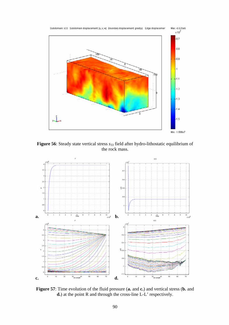
Figure 56: Steady state vertical stress s33 field after hydro-lithostatic equilibrium of

the rock mass.

a. b.

c. d. Figure 57: Time evolution of the fluid pressure (a. and c.) and vertical stress (b. and

d.) at the point R and through the cross-line L-L’ respectively.

90

6.3 Drifts excavation simulation Once the fractured rock mass is stabilized in the hidro-lithostatic steady state, we simulate the drifts excavation process. However, hydraulic conditions have been modified to approximate the real conditions existing at the Grimsel Test Site. On the other hand, although the FEBEX drift was excavated much later than the Grimsel access tunnels, we have simulated all the excavations simultaneously for simplicity. The excavation process has been simulated by gradually modifying the boundary conditions on the drift walls (called ‘constrains’ in the tables) from the rock steady state conditions to the tunnel conditions (P = 0 and s33 = 0). Boundary conditions are defined according to the nomenclature for the boundaries given in Figure 48, and with the help of the above logical expressions for the geometrical features in the domain. Tables 13 and 14 show the boundary conditions and the initial conditions and constrains respectively:

Table 11: Boundary conditions of the drifts excavation simulation.

B.C. A1 A2 B1 B2 C1 C2 Thermal - - - - - -

Hydraulic No flux

No flux

P=2.1 MPa

P=0.7 MPa

( )100

2007.0 yP −⋅=

( )100

2007.0 yP −⋅=

M

u=0m

w=0m

echanic u=0m u=0m v=0m v=0m v=0m σ33=365·ρeq·g

Table 12: Initial conditions and constrains of the drifts excavation simulation.


(FBXinst, FBXaux, LABtun, MAINtun)

Test zone (FBXheat)

Thermal - - -

Hydraulic ( )100

2007.0 yP −⋅= MPa P=0 Pa P=0 Pa

Mechanic u=0 m, v=0 m, w=0 m ni•σii =0 ni•σii =0 H-MODEL RESULTS

The initial conditions for the hydraulic head (Figure 58a) are given by the regional regime (Jüchlistock mountain and Aare river), which has very high gradients both vertical and horizontal, corresponding to the mountainous characteristics of the area and to the low permeability of the medium. The different sizes of the initial conditions flux arrows depend on the heteroteneous distribution of the intrinsic permeability. The heterogeneous anysotropic hydraulic model yields to the hydraulic head steady state of Figure 58b after the excavations for the cross-section X=4.6m. Typical hydrostatic pressure profile is strongly modified due to the imposed conditions in the excavated zones (P=0). As a consequence, flux is directed towards the drifts.

91

a.

b.

Figure 58: Cross-section A-A’ of the te steady closer detailed view of the te zone (b.).

the fluid pressure is presented in Figures 59a-d, in which th final

and two intermediate times are showed. Pressure below zero may be due to numerical

Figure 60 plots the isolines of the hydraulic head at steady state: Figure 60a plots the

n z=0, and Figure 60b plots the vertical cross-section A’-A th respect to previous figures). Hydraulic head values obtained

in hy

mperature field in the state (a.) and a st

Evolution of e inicial,

errors.

horizontal cross-sectio(oppositely oriented wi

draulic tests made in boreholes FEBEX-95001 and FEBEX-95002 before the excavation of the drift are also showed in red. The observation points closest to the FEBEX drift are the ones which present the highest discordance, due to the effects of the excavation on the hydraulic head field around the excavated zone. Results obtained by the UPC simulations (figures 3.12 and 3.13 of [34]) are similar, with slight differences in the local irregularities around the FEBEX drift. This is due to the homogenization performed in this model, alternatively to the inclusion of discrete fractures in the UPC models.

92

93

Fig fluid rifts excavation simulation. Four time instants are showed: a. Time t = 0 years; b.

Time day Time t = 45 days; d. Time t = 3.17 years.

pressu t = 22

re in the ds; c.

ure 59: Time evolution of the

94

a.

b. Figure 60: Hydraulic head isolines at steady state: a. Horizontal cross section at z=0;

b.: Vertical cross section A’-A. M-MODEL RESULTS

The isotropic case yields to the steady state for vertical stresses section A-A’ plotted in Figure 61. Accumulation of vertical compressiat the top and bottom of the excavated drifts. Vertical displacement occurs uniformly in the domain.

s33 along cross-ve stresses occurs

Figure 61: Vertical stress steady state for the isotropic mechanic model.

HM-MODEL RESULTS

The excavation of the drifts yields in the coupled HM model to the steady state showed in Figures 62 and 63. Both homogeneous and heterogeneous anisotropic/non-orthotropic conditions are compared. Figure 62a presents the vertical stress field along with the vertical displacement isosurfaces for the homogeneous case. Figure 62b presents the same results for the heterogeneous case. We can appreciate that consolidation in the FEBEX test zone (last 17 m of the FEBEX drift) is higher, due to the higher fracture density in this zone. Figure 63 displays the fluid pressure for the heterogeneous anisotropic case. Water flow towards the drifts can be also seen.

a.

b.

Figure 62: Vertical stress s33 and vertical displacement isosurfaces steady state for e HM drifts excavation simulation: a. Homogeneous anisotropic/non-orthotropic th

conditions; b. Heterogeneous anisotropic/non-orthotropic conditions.

95

Figure 63: Fluid pressure and water flow lines steady state for the HM drifts

excavation simulation with heterogeneous anisotropic/non-orthotropic conditions. 6.4 Heating experiment simulation The simulation of the heating experiment has been performed for two different cases: with excavated drifts and without excavated drifts (drifts filled up with concrete or some other material of similar conditions than the rock mass). The real conditions for the FEBEX experiment are with excavated drifts. In both cases, however, the test zone has been filled up with bentonite. We only show results of the simulation w h excavations. The boundary conditions of this new problem are defined for each case similar to those imposed in the previous problems. Initial conditions correspond to the corresponding steady states reached in the excavation simulation for each of the cases. Table 16 gives the initial conditions and the constrains of the problem.

Table 13: Boundary conditions of the heating experiment simulation.

B.C. A1 A2 B1 B2 C1 C2

it

Thermal T=13 ºC T=13 ºC T=13 ºC T=13 ºC T=13 ºC T=13 ºC Hydraulic No flux No flux No flux No flux No flux P=365·ρw·g Mechanic u=0m u=0m v=0m v=0m u=0m

v=0m w=0m

σ33=365·ρeq·g

96

Table 14: Initial conditions and constrains of the heating experiment simulation.


(FBXinst, FBXaux, LABtun, MAINtun)

Test zone (FBXheat)

Thermal T=13 ºC - 2

2

14.165100 rT ⋅

−= ºC

Hydraulic H-model steady state - -

Mechanic M-model steady state - - T-MODEL RESULTS

In the heating problem the three types of analyses (isotropic, homogeneous anisotropic/non-orthotropic and heterogeneous anisotropic/non-orthotropic) give the same result, as thermal coefficients are isotropic for all cases. The t 6 a, and m

mperature surpasses slightly the profile imposed (up to 100ºC), surely due to the umerical method used and mesh interpolation errors.

hermal steady state result through the cross section A-A’ is given in Figure a detail of the near-field of the heaters is given in Figure 64b. The maximu

4

ten

a.

b. Figure 64: Cross-section A-A’ of the temperature field in the final state (a.) and a closer detailed view of the test zone (b.).

97

The temperature evolution in the middle point of the second heater, R, is showed in Figure 65a. Profile L-L’ for different times is also showed in Figure 65b. Density varies with temperature in all the ther eating conditions assumed in our problems the decrease zon reference value. The R-point evolution of d Figures 65c and 65d.

mal models, anof density in the hot and L-L’ profile

d for the h es is about 3% of theensity are showed in

a. b.

c. d. Figure 65: Time evolution in the point R (left-hand side) and in the vertical crossline

L-L’ (right-hand side): (a.) and (b.) temperature; (c.) and (d.) water density. TM-MODEL RESULTS

Thermal stresses are produced in the heating zone of the drift. Figures 66a and 66b show the L-L’ profile of stresses at different times for the cases of isotropic and homogeneous non-orthotropic stiffness coefficients respectively. Both isotropic and non-orthotropic approximations produce increasing vertical stresses near the heaters. The stress jump due to thermal stresses is higher for the non-orthotropic conditions (≈10 MPa) than for the isotropic ones (≈6 MPa). In all cases, thermal stresses are much smaller than the stresses produced by the excavation of the drifts.

98

b.a. Figure 66: Vertical stresses s33 in the crossline L-L’ for different rock conditions: a.

isotropic stiffness tensor; b. homogeneous non-orthotropic stiffness tensor. THM-MODEL RESULTS Test zone of the FEBEX drift has been filled up with bentonite and the 3-year heating has been simulated. The steady state of the fluid pressure is showed in Figure 67, along with the horizontal components of the water flow at z = 0. Figure 68 presents the Von Misses stress, the hydraulic head isolevels and the deformed shape of the domain. Note the thermal stresses around the test zone and the influence of the boundary conditions for displacements on the cummulation of stress in the lower boundary. The displacements at steady state are also shown for the whole domain in Figure 69: horizontal displacements u (Figure 69a) and v (Figure 69a) and the vertical displacement w (Figure 69c). A detailed view of the FEBEX drift wit in e A-A’ cross-section is plotted for the different variables of the coupled processes: temperature T (Figure 70a), fluid pressure P7

shear rains ε23, ε13, ε12 (Figures 72d, 72e and 72f respectively) and displacements u, v, w

c respectively). In the Von Mises stress plot (Figure 70c), uled not only around the heaters, but also in the bentonite-

ck c

boreholes drilled out from the test zone of the FEBEX drift.

h th

(Figure 70b), Von Misses stress (Figure 70c), normal stresses s11, s22, s33 (Figures 71a, 1b and 71c respectively), shear stresses s , s , s (Figures 71d, 71e and 71f23 13 12

respecst

tively), normal strains ε11, ε22, ε33 (Figures 72a, 72b and 72c respectively),

(Figures 73a, 73b and 73hermal stresses are cummt

ro ontact, the last being due mainly to shear forces. In the cross-sections of the displacements (Figures 73a, 73b and 73c) we can appreciate how the bentonite expands both longitudinaly (displacement v) and radially (displacement w for this section) due to the heating process. As our interest here is in the simulation of the fractured rock, we have not explicitely compare our model with measurements taken in the bentonite. However, we do present some comparisons of the model with data coming from the radial

99

Figure 67: Final state of the fluid pressure. Flow at z=0 is also showed (only horizontal

components).

Figure 68: Final state of the Von Mises stresses, hydraulic head isolevels and deformed

shape of the domain.

100

a.

b.

c.

of the displacements uFigure 69: Final state (a.), v (b.) and w (c.).

101

a.

b.

c.

Figure 70: Detailed view of the THM final state of temperature (a.), fluid pressure (b.) and Von Mises stress (c.).

102

a.

b.

c.

Figure 71: Detailed view of the THM final state of normal stresses s (a.), s (b.) and ear stresses s (d.), s (e.) and

11 22s33 (c.) and sh 23 13 s12 (f.).

103

d.

e.

f.

Figure 71 (cont.): Detailed view of the THM final state of normal stresses s11 (a.), s22 and s(b.) f.). 33 (c.) and shear stresses s23 (d.), s13 (e.) and s12 (

104

a.

b.

c.

Figure 72: Detailed view of the THM final state of normal strains ε11 (a.), ε22 (b.) and ε33 (c.) and shear strains ε23 (d.), ε13 (e.) and ε12 (f.).

105

d.

e.

f.

Figure 72 (cont.): Detailed view of the THM final state of normal strains ε11 (a.), ε22 nd ε(b.) a f.). 33 (c.) and shear strains ε23 (d.), ε13 (e.) and ε12 (

106

a.

b.

c.

Figure 73: Detailed view of the THM final state of displacements u (a.), v (b.) and w (c.).

107

We have compared our results with field measurements of temperature, fluid pressure, total pressure and total displacements. Points of selected boreholes where data have been taken for comparison are showed in Figure 74:

• Temperature (red points): the selected boreholes are: a borehole drilled in a ‘hot’ section (closed to the second heater), SF23; a borehole drilled in a ‘cold section’ (far from heaters), SF14; and a borehole at the end of the FEBEX drift, SB22.

• Fluid (or interstitial) pressure (blue points): the selected boreholes are the SK1, inclined and crossing longitudinally the test zone, and the SJ5, at the end of the test zone, and the sampling points are showed in blue in Figure 74.

• Total pressure (green points): the selected boreholes are the two ones where this variable has been measured, SG1 and SG2.

• Total displacement (orange points): the selected boreholes are the two ones where this variable has been measured, SI1 and SI2.

Figure 74: Selected boreholes and sampling points for the temperature (red), intersticial pressure (blue) total pressure (green) and total displacements (orange) comparisons in the THM analysis

(original figure from [33]). Figure 75 shows the comparison of the measured and the simulated temperature in borehole SF23. The point closest to the bentonite (the hotest one) presents the higher discrepancy, whereas there is a good agreement for the other three points. Indeed, when considering the ‘cold’ boreholes SF14 (Figure 76) and SB22 (Figure 77), a good agreement between measured and simulated temperatures is found in all the sampling

nts. This is due to the imposed conditions to simulate the heating transient: instead of imposing a source term with a fixed heat flux, we have fixed a temperature profile withtemperature field in the nearest rock around the heaters.

poi

in the bentonite based on measured data. This probably underestimates the

108

a.

b.

c.

Figure 75: Time evolution of measured (x) and simulated (-) temperatures in boreholes SF23 (a.), SF14 (b.) and SB22 (c.) for the THM analysis.

109

Figure 76 displays the time evolution of the measured and the simulated intersticial (or fluid) pressure for the borehole SK1 (Figure 76a) and the borehole SJ5 (Figure 76b). As full saturation is assumed in the model, and may not be so in the near-field, some overestimation was expected to occur. However, both the large overestimation and the flat shape observed in the simulated fluid pressure are due to the initial conditions imposed in the simulation: full hydro-mechanical stabilisation of the rock mass and the bentonite filling the test zone were assumed. Doing so, the fluid pressure starts and ends at the same steady state value. No stabilisation should have been imposed, to lead the fluid pressure at the bentonite-rock mass contact start at zero (i.e. at the atmospheric pressure). Nevertheless, the transient peak observed in the meassured pressure around t=0.8·107 s is also reflected in the simulation. On the other hand, the fluid pressure measured at the borehole SJ5 is higher than the one measured at the borehole SK1, what confirms the coherence of the hydraulic gradient conditions imposed in the simulation.

a.

b.

Figure 76: Time evolution of measured (x) and simulated (-) fluid pressure in boreholes SK1 (a.) and SJ5 (b.).

110

Total pressure has been measured in two boreholes, SG1 (Figure 77) and SG2 (Figure 78), vertical and horizontal respectively, located at the middle section of the FEBEX drift test zone. There, sensors labelled from 01 to 05 are the furthest ones from the gallery (Figures 77a and 78a), and sensors from 06 to 10 are the closest ones (Figures 77b and 78b). We have compared the measured total pressure with the Von Mises stresses obtained in the model. Von Mises stress overestimates slightly the total pressure, although it gets the same order of magnitude. The thermal stresses resulting from the thermo-mechanical coupling occur fastly in the model than in the reality (see Figure 77b). This is surely due to a too high thermal conductivity in the rock mass, the same that caused the low temperatures in the sampling points closest to the heaters (see Figure 75a). On the other hand, the negative trend of the Von Mises stress at the long term, together with the high initial value, are due to the hydro-lithostatic steady state used as initial condition, as it was noticed for the fluid pressure. A new time analysis

ith the appropriate initial and boundary conditions would be convenient to clarify the behavior of the model in this aspect.

a.

w

b.

igure 77: Time evolution of measured (x) and simulated (-) total pressure in: a. Points from 01 to 05; b. Points fr

F borehole SG1 om 06 to 10.

111

a.

b.


Finally, total displacement measurements have been compared with the modulus of the displacement vector (u, v, w) in the direction of each selected borehole. The order of magnitude of the displacements is well simulated, but not the transient behaviour. Further studies are necessary to better interpret the total displacement measurements (they get negative values, for instance), and to be able to compare them correctly with the outputs of the simulation.

112

a.

b.

Figure 79: Time evolution of measured (x) and simulated (-) total displacements in boreholes SI1 (a.) and SI2 (b.).

113

7 CONCLUSIONS AND FUTURE WORK In the first part of the thesis, a comprehensive statistical methodology to analyse the time series coming from an experiment of coupled thermo-hydro-mechanical processes has been applied. Several techniques covering the time, space, frequency and scale frames of the measured data have been used, to obtain a qualitative and quantitative characterization of the physical processes occurring, unexpected events and general performance of the sensors installed within the experiment. Some of the most relevant results obtained in our study have been presented here, and are already published in [22] (full article in APPENDIX XIII). Firstly, concerning the physical processes occurring in the Mock-up test, an insight to the unpredicted slow down of the water intake and hydration rate of the bentonite has been offered: a decrease in the relative humidity gradient has been observed, and the hypothesis of the development of an evaporation-condensation cell has been analysed to explain the unpredicted behaviour. Secondly, a deep study of the overheating incident in the Mock-up has been done. No important consequences or irreversible perturbations of the processes or the sensors have been evidenced from the results obtained. Moreover, a quick recovery of the temperature normal measurements has been observed, being that of the humidity and pressure sensors a bit longer. Finally, a systematic study of the performance of all the sensors has been made, and results concerning an abnormal behaviour of some total pressure sensors has been presented. There has been seen that those sensors work correctly, but they measure the fluid pressure instead of the total pressure due to a lack of connectivity with the solid phase of the bentonite. The statistical methodology used in this work has demonstrated to be very useful to understand and characterize coupled processes and sensors reliability within this kind of experiments. Statistical techniques should be considered as an essential analysis tool, complementary to any modeling process, not only in the nuclear waste engineering, but also in any complex multidisciplinary engineering experiment. However, further work is necessary to better link the results of the statistical analyses with the modeling tasks. In the second part of the thesis, we have developed a methodology to simulate a 3D fractured network that fits optimally a cylindrical tunnel tracemap. The optimization procedure searches for the best parameters of the size distribution to minimize the discrepancies between measured and simulated trace length and 3D trace chord histograms and number of intersections with the tunnel and two exploratory boreholes. A good agreement between both fractured mediums has been found in the results. This methodology provides a good starting point for the use of cylindrical tracemaps to simulate geological 3D fractured networks, and completes the classical use of flat wall tracemaps that is more extensively developed in the literature.

115

Although satisfactor omments for future ork:

-

ature, because it depends on the generation of a fractured medium obtained with statistical distributions. This

average has to be determined according to the confidence interval needed in the objective function.

the third part of the thesis, a thermo-hydro-mechanical model has been developed and

ropic and heterogeneous homogenized coefficients have been sed for hydraulic, mechanic and thermal submodels. Variation of water properties with

- As stated before, the stochastic nature of the fractured medium generation

this would require an enormous computational effort, such that it would only be

as, for instance: non-saturated or partially saturated conditions, better coupling in the bentonite-rock contact, elastoplastic model, new cracks development, dependency of the fracture aperture on stress, etc.

y results have been obtained, here are some cw

The non-homogeneous fractured network simulated near the gallery could be assumed to be the same in the overall domain, so the statistical functions producing the fractured medium would be extended everywhere. To do that, non-homogeneous Poisson processes should be used [84], and some kind of density measure must be defined for every point in the 3D space. The reduced second moment function [42] of the tracemap could be used for this purpose.

- The objective function has a stochastic n

means that, for the same set of parameters Rmin, Rmax, and b, we can obtain different values of the objective function for each realization. Therefore, an average of the objective functions of several realizations should be used to obtain a more reliable value given a set of parameters. The number of realizations to use in that

- For a hydrological validation of the fractured medium, hydraulic and transport

tests available in the site should be used, with hydraulically conditioned fractured networks.

Inimplemented in Comsol Multiphysics®, and an up-scaling methodology has been defined to feed the model with homogenized coefficients. Several one-way and two-way couplings have been incorporated to the model: Biot hydro-mechanical coupling, thermal stresses, thermal expansion of water, and heat convection and conduction. Fully anisotropic / non-orthotutemperature has also been considered. The FEBEX experiment has been simulated with this model, with a good agreement between measured and simulated values of the main variables. Some remarks can be also made in this part for future work:

process makes necessary to compute it as an average of several realizations. Indeed, the objective function should be chosen not only based in morphological aspects of the fractured network, as it is made in this work, but also such that minimizes the discrepancies between the THM time-dependent model outputs and the field measurements as compared in the last part of chapter 6. However,

possible with the use of computer clusters or powerfull workstations. - Future enhancements of the model should incorporate new couplings between

the processes and generalize the material conditions

116

- The upscaling performed in the hydraulic coefficients could be generalized for

the mechanical and the thermal coefficients as well. By following a similar

Finamodel in the coeffic

reasoning, we could fix the global stress field (constant) and compute the strain by superposition of the individual contributions of each fracture to the total strain, given a ‘low-order’ boundary condition for stresses. Similarly, in the thermal model we could up-scale the coefficients by weighting with the fracture volumetric fraction of each homogenization subdomain, as the presence of fractures influences substantially the heat transport by conduction.

lly, in this work we have developed an integrated methodology to analyse and coupled processes in tridimensional fractured media, with special contributions simulation of the fractured network and in the upscaling of the hydraulic

ients.

117

8 REFERENCES

[1] Ababou R. Approaches to Large Scale Unsaturated Flow in Heterogeneous, Stratified, and Fractured Geologic Media. Report NUREG/CR-5743, U.S. Nuclear Regulatory Commission, Washington D.C., USA. Government Printing Office, pp.1-150, 1991.

[2] Ababou R. & L. W. Gelhar. Self-Similar Randomness and Spectral Conditioning: Analysis of Scale Effects in Subsurface Hydrology, Chapter XIV in Dynamics of Fluids in Hierarchical Porous Media, J. Cushman editor, Academic Press, New York, pp. 393-428. 1990.

[3] Ababou, R, Cañamón, I., Elorza, F.J. Thermo-Hydro-Mechanical Simulation of a 3D Fractured Porous Rock: Preliminary Study of Coupled Matrix-Fracture Hydraulics. Proceedings of the COMSOL Multiphysics Conference 2005, pp. 193-198. Ed. J. M: Petit and J. Daluz. France. November 2005.

[4] Ababou R., A. Millard, E. Treille, M. Durin, & F. Plas. Continuum Modeling of Coupled Thermo-Hydro-Mechanical Processes in Fractured Rock. Computational Methods in Water Resources (CMWR'94 Heidelberg), Kluwer Acad. Publishers, A. Peters et al. (eds.), Vol.1, Chap.6, pp.651-658. 1994.

[5] Ababou R., A. Millard, E. Treille, & M. Durin. Coupled Thermo-Hydro-Mechanical Modeling for the Near Field Benchmark Test 3 (BMT3) Of Decovalex Phase 2. CEA/DMT Progress Report 93/488. May 1994.

[6] Ababou R., A.C. Bagtzoglou, & E.F. Wood. On the Condition Number of Covariance Matrices Arising in Kriging, Estimation, and Simulation of Random Fields. Mathematical Geology, Vol. 26, No. 1, pp. 99-133. 1994.

[7] Alonso E., J. Alcoverro, F. Coste, L. Malinsky, V. Merrien-Soukatchoff, Kadiri, T. Nowak, H. Shao, T.S. Nguyen, A.P.S. Selvadurai, G. Armand, S.R. Sobolik, M. Itamura, C.M. Stone, S.W. Webb, A. Rejeb, M. Tijani, Z. Maouche, A. Kobayashi, H. Kurikami, A. Ito, Y. Sugita, M Chijimatsu, L. Börgesson, J. Hernelind, J. Rutqvist, C.-F. Tsang & P. Jussila. The FEBEX Benchmark Test: Case Definition and Comparison of Modelling Approaches. International Journal of Rock Mechanics & Mining Science. Ed. Elsevier. May 2005.

[8] Amiguet, J.L. Grimsel Test Site. Felskennwerte Von Intaktem Granit. Zusammen-Stellung Felsmechanischer Laborresultate Diverser Granitischer Gesteine. NAGRA, NIB 85-08, September 1985.

[9] Bacry, E, Mallat, S. & Papanicolaou, G. A Wavelet Based Space-Time Adaptive Numerical Method for Partial Differential Equations. Mathematical Modelling & Numerical Analysis 26: pp. 793-834. 1992.

[10] Baecher G.B., Einstein H.H. & Lanney N.A. Statistical Description of Rock Properties and Sampling. Energy Resources and Excavation Technology; proceedings, 18th U.S. Symposium On Rock Mechanics. Golden: Colo. Sch. Mines Press. Wang FD, Clark GB, editors. pp. 5C1.1–8. 1977.

[11] Barenblatt G., Zelthov I. & Kochina I. Basic Concepts in the Theory of Seepage of Homogeneous Liquids in Fissured Rocks, Journal of Applied Mathematics 24, 213-240. 1960.

119

[12] Beylkin, G & Coult, N. A rategy for Reduction of Elliptic PDE’s and Eigenvalue Problems. Program in Applied Mathematics. University

[13]

[15] ood Cliffs, New Jersey, 1994.

[17] dia 11, 263-280.

[18]

[22]

& Image

[24]

Multiresolution St

of Colorado at Boulder. 1998.

Biot, M.A. Theory of Deformation of a Porous Viscoelastic Anisotropic Solid. Journal of Applied Physics 27: pp. 459-467. 1956a.

[14] Biot, M.A. General Solutions of the Equations of Elasticity and Consolidation for a Porous Material. Journal of Applied Mechanics 23: pp. 91-96. 1956b.

Box, G.E.P., Jenkins, G.M. & Reinsel, G.C. Time Series Analysis: Forecasting and Control. Third Edition, Prentice Hall, Englew

[16] Bracewell, R.N. The Fourier Transform and its Applications. Mcgraw-Hill, Inc. USA. 1986.

Braester C. & Zeitoun D. Pressure Transient Response of Stochastically Heterogeneous Fractured Reservoirs, Transport in Porous Me1993.

Bräuer V., Kilger B. & Pahl A. Grimsel Test Site. Engineering Geological Investigations for the Interpretation of Rock Stress Measurements and Fracture Flow Tests. NAGRA, NTB 88-37E, April 1989.

[19] Brewster, M.E. & Beylkin, G. A Multiresolution Strategy for Numerical Homogenization. Applied & Computational Harmonic Analysis 2: pp. 327-349. 1995.

[20] Brockwell, P.J. & Davis, R.A. Introduction to Time Series and Forecasting. Springer-Verlag New York, Inc. 1996.

[21] Cañamón, I. & Paredes, C. The Applications of Wavelet Transform to Edge Detection and Fractal Analysis on Digital Terrain Elevation Models. Proceedings of the International Workshop on Fractal Mathematics Applied to Soil and Related Heterogeneous Systems ‘PedoFract04’, pp. 17-18. Spain. 2004.

Cañamón, I., Elorza, F.J., Mangin, A., Martín, P.L. & Rodríguez, R. Wavelets and Statistical Techniques for Data Analysis in a Mock-Up High-Level Waste Storage Experiment. International Journal on Wavelets, Multiresolution Processing 2(4): pp. 351-370. December 2004.

[23] Cañamón, I., Elorza, F. J., Ababou, R. 3D Fracture Networks: Optimal Identification and Reconstruction. Accepted for publication in the proceedings of the XIth IAMG Annual Congress. Belgium. September 2006.

Chan T., R. Christiansson, G.S. Boulton, L.O. Ericsson, J. Hartikainen, M.R. Jensen, D. Mas Ivars, F.W. Stanchell, P. Vistrand & T. Wallroth. DECOVALEX III BMT3/BENCHPAR WP4: the Thermo-Hydromechanical Responses to a Glacial Cycle and Their Potential Implications for Deep Geological Disposal of Nuclear Fuel Waste in a Fractured Crystalline Rock Mass. International Journal of Rock Mechanics & Mining Science. Ed. Elsevier. May 2005.

[25] Charton, P. & Perrier, V. A Pseudo-Wavelet Scheme for the Two-Dimensional Navier-Stokes Equations. Matemática Aplicada e Computacional 15: pp. 139-160 1996.

120

[26] CIEMAT. FEBEX (Full-Scale Engineered Barriers Experiment in Crystalline Host Rock): 21º Data Report. Mock-Up Test. Technical Report 70-Ima-L-9-101. Spain. 2002.

[27] Daubechies, I. Ten Lectures on Wavelets. CBMS-NSF Series in Applied Mathematics. SIAM. 1992.

[28] Dershowitz W.S & Einstein H.H. Characterizing Rock Joint Geometry with Joint System Models. Rock Mechanics & Rock Engineering 21(1):21–51. 1988.

.

[30] tal Analysis of Joint Patterns in Granite. International Journal of

[31] tividad (AGP). Diseños Conceptuales Genéricos. Technical Report Num.

[32] . Spain. 1996.

Num. 03/98. Spain. 1998.

rme de Síntesis. Technical Report Num.

[35]

[37] tures. Tectonophysics (226): pp.

[38] pp. 65-100.

[40]

al Characterization and Modeling. UPC. 70-UPC-M-0-1001. 1998.

[29] Dverstorp, B. & Andersson, J. Application of the Discrete Fracture Network Concept with Field Data: Possibilities of Model Calibration and ValidationWater Resources Research 25(3): pp. 540-550. March 1989.

Ehlen J. FracRock Mechanics & Mining Science 37(6): pp. 909–922. 2000.

ENRESA. Almacenamiento Geológico Profundo de Residuos Radiactivos de Alta Ac11/95. Spain. 1995.

ENRESA. FEBEX (Full-Scale Engineered Barriers Experiment in Crystalline Host Rock): Test Plan, Mock-Up Test. Version 1

[33] ENRESA. FEBEX (Full-Scale Engineered Barriers Experiment in Crystalline Host Rock). Diseño Final y Montaje del Ensayo “In-situ” en Grimsel. Technical Report

[34] ENRESA. FEBEX (Full-Scale Engineered Barriers Experiment in Crystalline Host Rock): Etapa Preoperacional. Info09/97. Spain. 1997.

Fadili A. & R. Ababou. Dual Homogenisation of Immiscible Steady Two-Phase Flow in Random Porous Media. Water Resources Research, Vol.40, W01513, DOI:10.1029 / 2003WR002465, 2004.

[36] Gasquet C. & Witomski, P. Analyse de Fourier et Application. Masson. Paris. 1995.

Gillespie, P.A., Howard, C.B., Walsh, J.J., & Watterson, J. Measurement and Characterization of Spatial Distributions of Frac112-141. 1993.

Goffe, Ferrier and Rogers, 1994. Global Optimization of Statistical Functions with Simulated Annealing. Journal of Econometrics (60, 1/2):

[39] Goodman R.E. Methods of Geological Engineering in Discontinuous Rocks. St. Paul: West Publishing Co. 1976.

Guimerá J., Ortuño F., Vázquez E., Ruiz B., Martínez L., Carrera J. & Meier P. Pulse Tests at ‘‘in Drift’’ Boreholes. Performance and Evaluation. UPC, 70-UPC-L-0-1001. 1996.

[41] Guimerá J., Carrera J., Martínez L., Vázquez E., Ortuño F., Fierz T., Bülher C., Vives L., Meier P., Medina A., Saaltink M., Ruiz B. & Pardillo J. FEBEX Hydrologic

121

[42] Hanisch, K.H. & Stoyan, D. Remarks on Statistical Inference and Prediction for a Hard-Core Clustering Model. Math. Operationsf. Statist., ser. statist. (14): pp. 559-567. 1983.

Fracture Networks Based on Regular Lattice

per J., Alonso E.

n. Report no EUR 19147 EN. 2000.

[48] . Inference of Discontinuity Trace Length

[49] in J., Schuler P. & Buletti M. Grimsel Test Site. Geology.

[50] d Mass Exchange Coefficient. ASME

[51] M., R. Ababou, B. Noetinger & M. Quintard. Coefficient D’échange

e Mécanique 332 (2004), pp. 679-686, Elsevier. 2004.

nal Of

[53] nd Simulation of Joints for Rock Engineering.

[55] of Interconnection to Permeability in Fractured Networks. Journal of Geophysical Research 90 (B4): pp. 3087-3098. 1985.

[43] Hestir, K. & Long, J.C.S. Analytical Expressions for the Permeability of Random Two-Dimensional PoissonPercolation and Equivalent Media Theories. Journal of Geophysical Research 95 (B13): pp. 21565-21581.

[44] Hudson J.A., O. Stephansson & J. Anderssond. Guidance on Numerical Modelling of Thermo-Hydro-Mechanical Coupledprocesses for Performance Assessment of Radioactive Waste Repositories. International Journal of Rock Mechanics & Mining Science. Ed. Elsevier. May 2005.

[45] Huertas F., Fuentes-Cantillana J.L., Jullien F., Rivas P., Linares J., Fariña P., Ghoreychi M., Jockwer N., Kickmaier W., Martinet M.A., Sam& Elorza F.J. Full Scale Engineered Barriers Experiment for a High-level Radioactive Waste in Crystalline Host Rock (FEBEX Project). Final Report. European Commissio

[46] Jenkins, G.M. Practical Experiences with Modeling and Forecasting Time Series. Gwilym Jenkins & Partners Ltd. Jersey. 1979.

[47] Jenkins, G.M. & Watts, D. G. Spectral Analysis and its Applications. Holden-Day. San Francisco. 1968.

Jiménez-Rodríguez R., N. SitarDistributions Using Statistical Graphical Models. International Journal of Rock Mechanics & Mining Science. Ed. Elsevier. February 2006.

Keusen H.R., GanguNAGRA, NTB 87-14E. 1989.

Kfoury M., B. Noetinger, M. Quintard, & R. Ababou. Upscaling in Fractured Heterogeneous Media: Permeability anJournal of Applied Mechanics (JAM). 2005.

KfouryMatrice-Fracture en Milieu Poreux Fracturé : Changement D’échelle Par Approche Stochastique. C.R.A.S. - Comptes Rendus de l'Académie des Sciences de Paris : C.R. d

[52] La Pointe, P.R. Derivation of Parent Fracture Population Statistics from Trace Length Measurements of Fractal Fracture Populations. International JourRock Mechanics & Mining Science (39): pp. 381-388. 2002.

La Pointe P.R. Pattern Analysis aComprehensive rock engineering. Volume 3—rock testing and site characterization. Oxford: Pergamon Press. Hudson JA, editor. pp. 215–239. 1993.

[54] Lewalle, J. Tutorial On Continuous Wavelet Analysis of Experimental Data. Siracuse University. 1995.

Long, J.C.S. & Witherspoon, P.A. The Relationship of the Degree

122

[56] Long, J.C.S. & Billaux, D. From Field Data to Fracture Network Modeling: an Example Incorporating Spatial Structure. Water Resources Research 23(7): pp. 1201-1216. July 1987.

[58] ’s Theorem Apply? Mathematical Geology 35(1): pp.

[59]

[61] sity. Technical Report.

[62] ystèmes Hydrologiques a

[68] aste Repository—a

[69] n T.S., A.P.S. Selvadura & G. Armand. Modelling the FEBEX THM

[57] Long J.C.S., Remer J., Wilson C. & Witherspoon P., Porous Media Equivalents for Networks of Discontinuous Fractures, Water Resources Research. 1982.

Lyman G.J. Stereological and Other Methods Applied to Rock Joint Size Estimation—Does Crofton9–23. 2003.

Mallat, S. A Theory for Multiresolution Signal Decomposition: the Wavelet Representation. IEEE Transactions on Pattern Analysis & Machine Intelligence 11 (7): pp. 674-693. 1989.

[60] Mallat, S. & Zhang, Z. Matching Pursuit in a Time-Frequency Dictionary. IEEE Transactions on Signal Processing 41, pp. 3397-3415. 1993.

Mallat, S. & Hwang, W.-L. Singularity Detection and Processing with Wavelets. Courant Institute of Mathematical Science. N.Y. UniverMarch 1991.

Mangin, A. Pour une Meilleure Connaissance des SPartir des Analyses Corrélatoire et Spectrale. Journal Of Hydrology, Amsterdam, Nº 67 pp. 25-43. 1984.

[63] Martín, P.L. Desarrollo y Diseño de Experimentos Aplicados a la Validación del Concepto Español de Almacenamientos de Residuos Radiactivos de Alta Actividad. Ph.D. thesis. Universidad Politécnica de Madrid. 2004.

[64] Mauldon M. Estimating Mean Fracture Trace Length and Density from Observations In Convex Windows. Rock Mechanics & Rock Engineering 31(4):201–16. 1998.

[65] Mauldon M. & Mauldon J.G. Fracture Sampling On a Cylinder: From Scanlines to Boreholes and Tunnels. Rock Mechanics & Rock Engineering 30(3):129–44. 1997.

[66] Metropolis, N., Rosenbluth, A., Rosenbluth, M., Teller A., and Teller, E. Equation of State Calculations by Fast Computing Machines. Journal of Chemical Physics. (21): pp. 1087–1092. 1953.

[67] Meyer, Y. Wavelets: Algorithms and Applications, SIAM. 1993.

Min K.B., J. Rutqvist, Chin-Fu Tsang & Lanru Jing. Thermally Induced Mechanical and Permeability Changes around a Nuclear WFar-Field Study Based On Equivalent Properties Determined by a Discrete Approach. International Journal of Rock Mechanics & Mining Science. Ed. Elsevier. May 2005.

NguyeExperiment Using a State Surface Approach. International Journal of Rock Mechanics & Mining Science. Ed. Elsevier. April 2005.

[70] Noorishad, J., Tsang C.-F., Stephansson O. & Jing L. Coupled thermo-hydro-elasticity phenomena in variably saturated fractured porous rocks : Formulation and numerical solution. Developments in Geotechnical Engineering: Coupled

123

Thermo-Hydro-Mechanical Processes of Fractured Media (O. Stephansson, L. Jing & C-F. Tsang, eds.) 79: pp. 93-134. Elsevier. 1996.

Oda. M. An Equivalen[71] t Continuum Model for Coupled Stress and Fluid Flow

[72] ock

[73] X (Grimsel-Suiza). CIEMAT, 70-IMA-M- 2-01. 1997.

[76] ater Resources 20(5-6): pp. 253-278. 1997.

[79] ck. Published

[80] Olivella, S. (directors).

[81] ch 5: pp. 1273-1289. 1969.

[83] d, A. Thoraval, & R. Ababou. ses of Fractured

[84] W.S. & Mecke, J. Stochastic Geometry and its Applications.

[85]

Analysis in Fractureed Rock-Masses. Water Resources Research, 22/13/, 1986.

Pahl A., Heusermann S.T., Bräuer V., Glöggler W. Grimsel Test Site. RStress Investigations. NAGRA, NTB 88-39E. 1989.

Pardillo J., Campos R. & Guimerá J. Caracterización Geológica de la Zona de Ensayo FEBE

[74] Polikar, R. The Wavelet Tutorial. Rowan University, College of Engineering (Http://Engineering.Rowan.Edu/~Polikar/Wavelets/Wttutorial.Html). 2001.

[75] Quintard M. & Whitaker S., Transport in Chemically and Mechanically Heterogeneous Porous Media: Theoretical Development of Region Averaged Equations for Slightly Compressible Single-Phase Flow, Advances in Water Resources 19, 29-47. 1996.

Renard, P. & de Marsily, G. Calculating Equivalent Permeability: a Review. Advances in W

[77] Resnikoff, H. L. & Wells, R. O. Jr. Wavelet Analysis (The Scalable Structure of Information). Springer – Verlag New York, Inc. 1998.

[78] Rutqvist, J. & Stephansson, O. The Role of Hydromechanical Coupling in Fractured Rock Engineering. Hydrogeology Journal 11: pp. 7-40. 2003.

Sahimi M. Flow and Transport in Porous Media and Fractured Roby VCH. 1995.

Sanchez, M. J. Thermo-Hydro-Mechanical Coupled Analysis in Low Permeability Media. Ph.D. thesis. Gens, A. & Departament D'enginyeria Del Terreny, Cartogràfica I Geofísica. UPC. 2004.

Snow, D.T. Anisotropic Permeability of Fractured Media. Water Resources Resear

[82] Steck, A. Die Alpidischen Strukturen in den Zentralen Aare-Graniten des Westlichen Aarmassivs. Eclogae geol. Helv. (61): pp. 19-48. 1968.

Stietel A., A. Millard, E. Treille, E. VuilloContinuum Representation of Coupled Hydro-Mechanical ProcesMedia: Homogenisation and Parameter Identification. Developments in Geotechnical Engineering: Coupled Thermo-Hydro-Mechanical Processes of Fractured Media (O. Stephansson, L. Jing & C-F. Tsang, eds.), 79:135-164, 1996, Elsevier.

Stoyan, D., Kendall, J. Wiley & Sons. 1987.

Strang G. & Nguyen, T. Wavelets and Filter Banks. Wellesey – Cambridge Press. 1997.

[86] Terzaghi, V.K. The Shearing Resistance of Saturated Soils and the Angle between the Planes of Shear. First International Conference of Soil Mechanics, Vol. 1: pp. 54-56. Harvard University. 1936.

124

[87] tor. Water Resources

[88] -

[89] rated Conditional Global

[92] Mechanical Characterization of a Bentonite from

International Meeting on

T3. INERIS Report, 1993.

6.

[96] vior of naturally fractured reservoirs. Society

[97] ship Between

Tompson A.F.B., R. Ababou, L.W. Gelhar. Implementation of the Three-Dimensional Turning Bands Random Field GeneraResearch, 25(10), pp. 2227-2243. 1989.

Trefethen, L.N. Pseudospectra of Linear Operators. SIAM Review 39, pp. 383406.

Tran, N.H., Chen, Z. & Rahman, S.S. IntegOptimisation for Discrete Fracture Network Modelling. Computers & Geosciences 32: pp. 17-27. 2006.

[90] Vetterli, R., O. & M. Wavelets and Signal Processing, IEEE Signal Processing Magazine, P.14-38. 1991.

[91] Villaescusa E. & Brown E.T. Maximum Likelihood Estimation of Joint Size from Trace Length Measurements. Rock Mechanics & Rock Engineering 25(2):67–87. 1992.

Villar M.V. Thermo-Hydro-Cabo de Gata. A Study Applied to the Use of Bentonite Sealing Material in High Level Radioactive Waste Repositories. Ph.D. Dissertation and ENRESA Technical Publication 01/2002, Madrid. 2002.

[93] Villar M.V. & Lloret A. Temperature Influence on the Hydromechanical Behavior of a Compacted Bentonite. Proceedings of theClays in Natural and Engineered Barriers for Radioactive Waste Confinement, Reims. 2002.

[94] Vuillod E. & A. Thoraval. Thermo-Hydro-Mechanical Coupled Modeling in the Near Field - BM

[95] Warburton P.M. Stereological Interpretation of Joint Trace Data: Influence of Joint Shape and Implications for Geological Surveys. International Journal Of Rock Mechanics & Mining Science Geomech Abstracts 17(6): pp. 305–311980.

Warren, J.E. & Root P.J. The behaof Petroleum Engineers Journal, pp. 245-255. Trans., AIME, 228. 1963.

Zhang L., Einstein H.H. & Dershowitz W.S. Stereological RelationTrace Length and Size Distribution of Elliptical Discontinuities. Géotechnique 52(6): pp. 419–33. 2002.

125

9 APPENDICES

127

129

APPENDIX I: Fractal Characterization of the FEBEX Tracemap This APPENDIX characterizes the fractal dimension of the FEBEX tracemap, as an alternative to build the fractured medium from a fractal model, instead of the Poisson model used in the thesis (for the fracture centers). Fractal dimension of the FEBEX area has been estimated by using the traces map of the FEBEX drift. We have implemented an algorithm of edge detection based on the wavelet transform [61]. This algorithm extracts the lineaments of an image through different scales by using the 2D multiresolution analysis, and we compute the fractal dimension with a Box-counting process on each image. For more details on the description of this technique see [21]. In our case, the fractal dimension has been estimated in D=1.70 (2.70 translated into 3D). Figure A-1 shows the different stages of the fractal dimension estimation algorithm and the final result of the estimation. Same estimation of fractal dimension has been performed separately in the five different zones in which geological reports divided FEBEX drift (see Figure 18). The two last zones, which were chosen to install the FEBEX experiment, have the highest values of fractal dimension, due to their higher fracture densities. This may be used for future generations of the fractured medium with fractal models. Figure A-2 shows the results of those estimations.

a. b.

c. d.

Figure A-1: Algorithm to estimate the fractal dimension of the FEBEX fractured

area: a. Original image of the traces map of FEBEX drift; b. Bidimensional MRA of the image; c. Modulus, phase and 95% of highest modulus values; d. Estimation of

fractal dimension from the modulus.

ZONE 1 ZONE 2 ZONE 3 ZONE 4 ZONE 5

D1=-1.6162 D2=-1.6800 D3=-1.4383 D4=-1.8205 D5=-1.762Figure A-2: Fractal dimension estimation for the five different zones of the FEBEX

drift. However, it is still an opened question whether if the fractal dimension of a curve image (cylindrical surface of the FEBEX drift developed in a plane) is equivalent to that of a planar image or not, or if it exists any relation between them that could be used to convert the calculated value.

130

APPENDIX II: Orientation Angles for a Planar Fracture in 3D Space

e referred to the Geographi rred to the FEBEX drift

cal solution of the in planar disk fracture and a cylindrical tunnel requires the use of several coordinated systems.

direction, both m respect to aphic North

In the simulation of the fractured medium of Chapter 4, some field data arc North, whereas some other are refe

local coordinated system. Additionally, analyti tersection of a

This APPENDIX clarifies the notations followed for the fracture vectors and angles. A planar fracture ‘F’ in 3D is defined geographically by its direction and plunge. We can alternatively define the dip (direction of the maximum slope), instead of the fracture

easured with the Geogr N . In our case, N c re geom r

normal to the plane containing that fracture. Taking the center of the fracture as the

oincides with the –X direction. On the other hand, we define the same planar fractuetrically by means of its center (a 3-coordinates point in the space) and the vecto

nF

origin of the coordinate reference system, the 3 components of the normal vector are defined in terms of the angles formed with the coordinate axes. The following relations hold for the different angles defining a planar fracture in 3D:

ϕλθβ

=−=180

(A-1)

where β dip, angle formed by the projection of Fn in the XY plane (called in

Figure A-3) and the –X direction (Geographic North). λ plunge, angle formed by the projection of

Fu

Fn in the fracture plane (called in Figure A-3) and the XY plane.

θ angle formed by the vectorFv

Fu and the +X direction. ϕ angle formed by the normal vector Fn and the +Z direction.

ϕ

y

x

z

θ

nF

cosθsinϕnF = sinθsinϕ cosϕ

N

β

uF

vF

λ

N ≡ Geographic Northβ = (N, uF) ≡ dip λ = (uF, vF) ≡ plungenF ⊥ vF

≡

≡

Figure A-3: Angles criteria for the 3D planar fractures used in the thesis.

131

APPENDIX III: Intersection of a Circular Fracture with a Cylindrical Tunnel

The analytical solution of the intersection of a planar disk fracture with a cylindrical excavation is presented here, as it is needed to perform the optimization/reconstruction of the fractured network of Chapter 4.2. To define analytically the equation of a trace produced by the intersection of a circular fracture on a cylindrical tunnel, we have to solve the system of equations formed by the cylindrical tunnel equation and the circular fracture (disk) equation in 3D. Three different coordinated systems have been considered:

o Absolute coordinated system XYZ: in which the Geographical North points towards the direction –X.

o Tunnel relative coordinated system XtYtZt: we have identified the origin of

this coordinated system with the previous one for simplicity, even if in the FEBEX project it is different. The +Xt axis forms an angle of 80º with the +X axis (FEBEX drift direction of N-260-E).

o Fracture relative coordinated system XfYfZf: the –Xf points towards the dip

direction within this system.

Figure A-4a shows schematically these three reference systems for a given fracture. There could be considered an additional coordinated system XtrYtr, as a result of the development of the cylinder in a 2D plane, the so called ‘tracemap’, which is shown in Figure A-4b. The system of equations mentioned above is:

2 2 2

2 2 2

, 2 2, 0

t tt t t t

f f f f

L Ly z R x

x y R z

⎧ + = − ≤ ≤⎪⎨⎪ + ≤ =⎩ (A-2)

being Rt ≡ tunnel radius, Lt ≡ tunnel length and Rf ≡ fracture radius. To solve the system of equations (A-2), we have to express all the equations in terms of the same coordinated system. Using the angles θ and ϕ defined in APPENDIX II for fracture ‘f’, and being (xfc, yfc, zfc) the coordinates of the fracture center, let’s write the equations in terms of the tunnel coordinated system with the aid of the corresponding rotation matrices (see APPENDIX VIII): ROTATION FROM (X, Y, Z) TO (Xf, Yf, Zf)

cos cos sin cos sin

, sin cos cos sin sinsin 0 cos

f

f

f

x xy A y Az z

θ ϕ θ θ ϕθ ϕ θ θ ϕ

ϕ ϕ

⎛ ⎞ −⎛ ⎞ ⎛ ⎞⎜ ⎟ ⎜ ⎟ ⎜ ⎟= ⋅ = −⎜ ⎟ ⎜ ⎟ ⎜ ⎟

⎜ ⎟ ⎜ ⎟⎜ ⎟ ⎝ ⎠ ⎝ ⎠⎝ ⎠

(A-3)

133

RO

TATION FROM (Xt, Yt, Zt) TO (X, Y, Z)

( ) ( )( ) ( ), sin 260º 180º cos 260º 180º 0

0 0

t

t

t

y B y Bz z

⎜ ⎟⎜ ⎟ ⎜ ⎟= ⋅ = − − −⎜ ⎟⎜ ⎟ ⎜ ⎟⎜ ⎟ ⎜ ⎟ ⎜ ⎟⎝ ⎠ ⎝ ⎠ ⎝

(A cos 260º 180º sin 260º 180º 0

1

x x − −⎛ ⎞⎛ ⎞ ⎛ ⎞

⎠

-4)

Adding up the two rotation matrices (3.2) and (3.3), yields to ROTATION FROM (Xt, Yt, Zt) TO (Xf, Yf, Zf)

(cos cos cos80º (cos cos sin80ºsin

cos sin sin80º ) cos sin cos80º )t tx x

(sin cos80º (sin sin 80º, 0

f

f t

f

xy A B y C y Cz

ϕ θ ϕ θ

cos sin80º ) cos cos80º )( sin cos cos80º

sin s

t

t tz z

ϕϕ θ ϕ θ+ −

⎛ ⎞ ⎛ ⎞⎜ ⎟ ⎜ ⎟ θ θ

+ −

⎛ ⎞− +⎜ ⎟

⋅ = ⋅ ⋅ =⎜ ⎟⎜ ⎟⎝ ⎠

θ θϕ θ

ϕ

⎜ ⎟ ⎜ ⎟ − +⎜ ⎟ ⎜ ⎟⎝ ⎠ ⎝ ⎠ − −

−( sin cos sin80º

cosin sin80º ) sin sin cos80º )

ϕ θ

= ⋅

ϕθ ϕ θ

⎜ ⎟⎜ ⎟− +

⎛ ⎞

⎟⎜ ⎟

⎜ ⎟⎜ ⎟⎜

⎜ ⎟⎜ ⎟

(A-5)

+⎝ ⎠

a.

b.

Figure A-4: a. Disk fracture intersection with a cylindrical tunnel

in 3D and b. Trace formed in the tunnel wall developed in 2D.

134

Considering also the translation and rotation of the fracture center (origin of the fracture coordinated system), we can express the fracture coordinates as:

( ) ( ) ( )( ) ( ) ( )

11 12 13

21 22 23

f t fc t fc t fc

f t fc t fc t fc

x c x x c y y c z z

y c x x c y y c z z

⎫= − + − + −

( ) ( ) ( )31 32 33f t fc t fc t fcz c x x c y y c z z

⎪⎪= − + − + − ⎬⎪

(A-6)

= − + − + − ⎪⎭ Introducing (3.5) into (3.1) yields to

( ) ( ) ( ) ( ) ( ) ( )2 22 211 12 13 21 22 23f f t fc t fc t fc t fc t fc t fcx y c x x c y y c z z c x x c y y c z z⎡ ⎤ ⎡+ = − + − + − + − + − + −⎣ ⎦ ⎣ ⎤ =⎦

(A-7)

where

)

⎡ ⎤+ + + +⎣ ⎦

2 2 2 0t t t t t t t t t t t tAx By Cz Dx y Ex z Fy z Gx Hy Iz J= + + + + + + + + + ≤

( )( )( )

( ) ( ) ( )

( ) ( ) ( )

2 211 21

2 212 22

2 213 23

11 12 21 22

11 13 21 23

12 13 22 23

2 211 21 11 12 21 22 11 13 21 23

2 211 12 21 22 12 22 12 13 22 23

11 13

2

2

2

2

2

2

fc fc fc

fc fc fc

A c c

B c c

C c cD c c c c

E c c c c

F c c c c

G c c x c c c c y c c c c z

H c c c c x c c y c c c c z

I c c

= +

= +

= +

= +

= +

= +

⎡ ⎤= − + + + + +⎣ ⎦⎡ ⎤= − + + + + +⎣ ⎦

= − +( ) ( ) ( )( ) ( ) ( ) ( ) (

2 221 23 12 13 22 23 13 23

2 2

11 13 21 11 13 21 23 21 22 23

fc fc fc

fc fc fc fc t t fc t fc

c c x c c c c y c c z

J c x c y c z c x c c c c x c y y c z z

⎧⎪⎪⎪⎪⎪⎪⎪⎪⎨⎪⎪⎪⎪⎪⎪⎪⎪ ⎡ ⎤= + + + + + − + − + −⎣ ⎦

(A-8)

o the final system of equations to be solved is

⎩ S

( ) ( ) ( )

2 2 2

31 32 33

2 2 2

, 2 20

0Ax

t tt t t t

t fc t fc t fc

t t t t t t t t t t t t

L Ly z R x

c x x c y y c z z

By Cz Dx y Ex z Fy z Gx Hy Iz J

⎧ + = − ≤ ≤⎪⎪ − + − + − =⎨⎪

+ + + + + + + + + ≤⎪⎩

(A-9)

he solution of this system of equations yields to the analytical equation defining the ace, and if we solve it with equality in the third equation we get the extreme points of e trace. Plane circular fractures intersecting with a cylindrical wall produce complete

r uncompleted elliptical-shaped traces. Depending on the number of solutions of (A-9) hich depend in fact of the size and orientation of the fracture with respect to the

nnel), four ferent general cases of intersection can be found (see Figure A-5).

Ttrtho(wtu dif

135

a.

A

B

b.

A

BC

D

c. d.

Figure A-5: Different types of intersections between a disk fracture and a cylindrical tunnel in 3D depending on the number of solutions of the

equations system: a. Uncomplete trace (two extreme points); b. Uncompleted trace (four extreme points); c. Complete trace (zero extreme points); and d.

No trace (zero extreme points).

136

APPENDIX IV: Detailed Results of the Fractured Medium Optimization

We present in this APPENDIX a more detailed version of the results of the fractured medium optimization presented in Chapter 4.2. We rec that the optimization process was com sed by 2 succesive steps (see Chapter 4.2.2). STEP 1: OPTIMIZATION AVERAGES OF 3 EVALUATIONS

Due to the stochastic nature of the fractured media generated with statistical distribution functions, a given set of values for these functions can yield to different fractured networks depending on the alleatory seed used to generate them. For this reason, on each iteration of the optimization process (a fixed set of parameters), we compute the objective function (OF) value as the average of the values obtained for 3 different fractured media (different alleatory seeds). Doing so, we minimize the dependence of the results on the alleatory seed. The initial values for the Pareto distribution set of parameters, PARETOini=(Rmin, Rmax, b)ini , and the corresponding search interval for each of those parameters, SINTini, have been: PARETOini = (1, 100, 2) SINTini = (1, 0, 1) (A-10) Figure A-6 presents the evolution of the OF in the optimization process, where only the enhanced values have been plotted: 368 it tions have been necessary to reac the optim m. Table A-1 shows the values of th ptimum set of parameters found, as well as th O igures A-7 sh one: Figur the cumu the tracem

Figure A-6: Evolution of the objective function (OF) in the first step of the optimization process.

allpo

WITH

era he ou

e F value and the number of fractures of the optimized fractured medium. Fow a comparison of the simulated fractured medium and the measured

e A-7a plots the cumulative histograms of the trace lengths; Figure A-7b plotslative histograms of the 3D trace chords; and Figures A-7c and d displayaps generated on the drift wall.

0

5

10

15

20

25

30

35

40

0 100 200 300 400

OF

iteration

137

Table A-1: Main characteristics of the optimum fractured medium obtained in the

first step of the optimization process.

# of fractures Rmin Rmax b OF

2813731 0,19851 100 3,3048 0,55917

b. a.

c.

d.

e.

f.

Figure A-7: First step optimization: a. Cumulated distribution function of trace lengths on tunnel (⎯ observed; ---- fitted); b. Cumulated distribution function of chord lengths on tunnel (⎯ observed; ---- fitted); c. FEBEX drift observed tracemap; d. FEBEX drift

fitted tracemap; e. Observed tracemap detail; and f. Fitted tracemap detail.

138

STEP 2: BEST REALIZATION OF 750 WITH OPTIMA PARAMETERS In the second step of the f 750 realizations of the fractured medium with the optimum arameters found in step 1, changing the alleatory s , jective function value has been ameliorated with respect to the f

FO = 0.4651 = 0.0525 + 0.0493 + 0.0931 + 0.0050 + 0.1843 + 0.0810 (A-11)

(decomposition of the OF in the different contribution terms is described in chapter 4.2.2) The 35-elements long vector of the alleatory seed corresponding to the optimum fractured medium is also given for results reproduction purposes:

Seedopt = (0.0453, 0.2314, 0.7191, 0.5697, 0.0413, 0.1733, 0.1024, 0.8156, 0.4372, 0.2802, 0.4669, 0.6666, 0.6525, 0.2039, 0.8377, 0.6420, 0.9931, 0.4040, 0.0103, 0.7557, 0.2186, 0.3339, 0.5347, 0.0721, 0.8249, 0.6506, 0.7555, 0.8487, 0.8015, 0.3614, 0.4406, 0.7144, 0.000, 0.000, 0.000)

S ilarly to step 1, Figure A-8 presents in the optimization process, where only the enhanced values have been plotted: the realization 554 gets the best result of the OF. Table A-2 shows a comparison of the characteristics of the optimum fractured medium and the field measurements. Figures A-9 show a c arison of the simulated fractured medium and the measured one: Figure A-9a plots the cumulative histograms of the trace lengths; Figure A-9b plots the cumulative histograms of the 3D trace chords; and Figures A-9c and d display the tracemaps generated on the drift wall.

Table A-2: Main characteristics of the optimum fractured medium obtained in the second step of the optimization process and comparison with the measured values.

Measured Simulated

optimization we obtain the best out o p

eed. In this step the obirst one:

im the evolution of the OF

omp

Number of fractures - 2906474 Number of tunnel traces 614 800 Number of intersections with borehole FEBEX-95001

155 144

Number of intersections with borehole FEBEX-95002

410 234

Volumetric density ρ32 - 2.9816 Areal density ρ21 1.4933 1.9182 Areal density ρ21 in zone 1 1.1544 1.4301 Areal density ρ21 in zone 2 2.0964 2.5298 Areal density ρ21 in zone 3 0.7961 1.2622 Areal d 21ensity ρ in zone 4 2.0825 2.6892 Areal density ρ21 in zone 5 3.0774 3.3651

139

Figure A-8: Evolution of the objective function (OF) in the second step of the optimization process.

a. b.

c.

d.

e. f. Figure A-9: Second step optimization: a. Cumulated distribution function of trace

lengths on tunnel (⎯ observed; ---- fitted); b. Cumulated distribution function of chord lengths on tunnel (⎯ observed; ---- fitted); c. FEBEX drift observed tracemap; d.

FEBEX drift fitted tracemap; e. Observed tracemap detail; and f. Fitted tracemap detail.

0,4

0,5

0,7

0,65

0,45

0,55

0,6

0 100 200 300 400 500 600 700

OF

iteration

140

APPENDIX V: Pseudo-Spectral Method for the 1-D Advection-Diffusion Equation

This APPENDIX describes an efficient numerical method to solve the advection-diffusion equation the based on the Fourier transform, which was thought initially as a way to further use the multiscale wavelet-based algorithms for solving the PDE’s of the T-H-M model of Chapter 6. 1-D MODEL FOR THE ADVECTIVE-DIFFUSIVE EQUATION WITH VARIABLE COEFFICIENTS

A 1-D m del solving the advection-diffusion equation with time and space variable coefficie t en developed. The same algorithm c epending on the

lution). The equ ed in the Fourier ansform.

The advection-difusion equation with variable coefficients can be written:

on s (flux velocity and diffusion coefficient) has bean be applied for the non-linear case (coefficients dation is solved by a pseudo-spectral method [88] basso

tr

2

2 ),(),(),(),(),(

xd

txudtxDxd

txdutxvdt

txdu⋅+⋅= (A-12)

where ( )txu , is the dependent variable (for instance, concentration), x is the position vector, and t the time. The first term of the right hand side represents the advective transport, with advective velocity ( )txv , , and the second term represents the diffusive

transport, where the diffusion coefficient is given by the tensor ( )txD , . This equation has been applied to a unidimensional periodic domain x = [0, L]. Thus, for an initial value u0 we have:

⎪⎪⎪

⎩

⎪⎪⎪

⎨

⎧

==

⋅+⋅=

0

2

2

)0,(),(),0(

),(),(),(),(),(

uxutLutu

dxtxudtxD

dxtxdutxv

dttxdu

(A-13)

PSEUDO-SPECTRAL METHOD FOR THE RESOLUTION OF PDE’s The pseudo-spectral method applied to the resolution of Partial Differential Equations (PDE’s) is based in the Fourier interpolation concept. For a given function u(x) ∈ R, we can define an algorithm to interpolate it in an infinite domain by the following steps:

- Considering its orthogonal projection vj on Z, which can be considered as a discretization of the real line (see Fi A-10). gure - Performing the Fourier transform ( )ξv of the discretized function vj:

( ) ∑+∞

∞−

∆−∆= jxji vexv ξξˆ (A -14)

141

u(xj) = vj

(xj = j·∆x)

Figure A-10: Discretization of a function f(x)∈R in Z.

- Substituting in the exact inverse Fourier transform of u(x) the values of its transform ( )ξu by the approximated values ( )ξv , which correspond to the u(x) transform performed uniquely in the discretization points xj:

Exact value: ( ) ( )∫∆

∆−

= x

x

duexu xiπ

πξξ

πξ ˆ

21 (A-15)

Approximated value: ( ) ( )∫∆

∆−

= x

x

dvexu xiπ

πξξ

πξ ˆ

21~ (A-16)

Remark: this approximation can also be considered as an interpolation of the u(xj) values, because ( )ξv is a continuous function although it only contains information of the xj points. Substituting the values of ( )ξv in the previous integral expresión:

( )

( )

( )

( )

( )

( )∑

∑

∑ ∫

∫ ∑

∞+

∞−

∞+

∞− −

−

−

∞+

∞−−

−

−

+∞

∞−

−

−∆

⎟⎠⎞

⎜⎝⎛ −

∆=

=⎥⎦

⎤⎢⎣

⎡∆=

=∆

=

=⎟⎠

⎞⎜⎝

⎛∆=

∆

∆

∆

∆

∆

∆

j

j

j

xxi

xxi

j

xxij

jxixi

xxx

xxxv

evx

devx

dveexxu

x

x

j

j

x

x

j

x

x

j

π

π

π

ξπ

ξπ

π

π

π

π

π

π

ξ

ξ

ξξ

2

sin2

2

2

2~

(A-17)

We obtain finally:

( ) ( ) ( )( ) ( )x

x

xx

xx

xSvxxSxu jj ∆=∆

∆=−= ∑∞+

∞−

ππ

πcsin

sinwhere,~ (A-18)

∆x

142

This function sinc(πx/∆x) provides an exact interpolator of function u(x) in the points xj.

Correspondingly, an analogue expresión can be obtained for the Fourier interpolator in the case of a periodic finite domain of N+1 points, as the one we are loking for:

( ) ( ) ( )( )

⎟⎠⎞

⎜⎝⎛

∆

+

−

2tan2

2x

x

xN

N π∆=−= ∑

sinwhere,~ 2 xxSvxxSxu NjjN

π (A-19)

Once an interpolator of function u(x) has been defined, we can approximate the different differential operators present in the EDP’s for their resolution. To do that, it is enough to apply the operators to the approximated function ( )xu~ . In the advection-diffusion quation, thoe se operators are:

• Advective operator:

( )( )xudxduu

dxdu

xx~~ =→=

(A-20)

Substituing ( ) ( )∑+∞

∞−

−= jj vxxSxu~ we have:

( ) ( ) ( )( )∑∑+∞

∞−

+∞

∞−

−=⎟⎠

⎞⎜⎝

⎛−= jjkjjkkx vxxS

dxdvxxS

dxdxu~ (A-21)

And performing the corresponding derivative we get the final result:

( ) ( )

( ) ( )

⎪⎩⎟⎠

⎜⎝ 2

tan2⎪

⎪⎪⎨

⎧

≠⎞⎛ −

−

=

=

=

−

+∞

∞−∑

jkjk

jk

D

vDxu

jk

jkN

jjkNkx

if1

if0

with

~

,

,

(A-22)

Where (DN)k,j is a Toeplitz matriz with the following structure:

143

1 10 ................22 tan 2 tan

2 2............................................................................

1

2 tan2.......

1 1...22 tan 2 tan

2 2

N

x x x

Dx x

− −∆ ∆ ∆⎛ ⎞ ⎛ ⎞ ⎛ ⎞

⎜ ⎟ ⎜ ⎟ ⎜ ⎟⎝ ⎠ ⎝ ⎠

−=

∆ ∆⎛ ⎞ ⎛⎜ ⎟ ⎜⎝ ⎠ ⎝

⎝ ⎠......................

1 10 ...22 tan 2 tan

2 2.........................................................................................................

1 1 1................

x x∆ ∆⎞ ⎛ ⎞ ⎛ ⎞⎟ ⎜ ⎟ ⎜ ⎟⎠ ⎝ ⎠ ⎝ ⎠

− −

−

22 tan 2 tan 2 tan2 2 2x x x∆ ∆ ∆⎛ ⎞ ⎛ ⎞ ⎛

⎜ ⎟ ⎜ ⎟ ⎜⎝ ⎠ ⎝ ⎠ ⎝

0

⎡ ⎤⎢ ⎥⎢ ⎥⎢ ⎥⎢ ⎥⎢ ⎥⎢ ⎥⎢ ⎥⎢ ⎥⎢ ⎥⎢ ⎥⎢ ⎥⎢ ⎥

⎢ ⎥⎢ ⎥⎣ ⎦

(A-23)

• D

⎢ ⎥⎢ ⎥

⎞⎟⎠

iffusive operator:

( )( )xudxduu

dxud

xxxx~~

2

22

2 =→= (A-24)

Computing the corresponding second derivative, we obtain, in an way, the final expression for this

(

analogue operator:

( ) ( )( )=+∞

∞−∑ vDxu jjkNkxx

~,

2

) ) ( )(

( )⎪⎪⎪

⎩

⎪⎧

≠⎟⎠⎞

⎜⎝⎛ ∆−

=−∆

−

jkxjk

jkx

DN if

2sin2

if61

3

2

2

2π (A-25)

Where (DN

(2))k,j is also a Toeplitz matrix (remark that DN(2)

≠(DN)2):

⎪⎪⎨ −= ++ jk

jk 1with 1,

2

( )

2

22 2

2

1 1 1 1...................23 6 2sin 2sin 2 tan

2 2 2...................................................................................................................

N

x x xx

D

π⎛ ⎞− −−⎜ ⎟ ∆ ∆ ∆∆ ⎛ ⎞ ⎛ ⎞ ⎛ ⎞⎝ ⎠ ⎜ ⎟ ⎜ ⎟ ⎜ ⎟

⎝ ⎠ ⎝ ⎠ ⎝ ⎠

=2

22 2 2 2

...........

1 1 1 1 1... ...2 23 62sin 2sin 2sin 2sin

2 2 2 2.........................................................................................

x x x xxπ⎛ ⎞− − −

−⎜ ⎟∆ ∆ ∆ ∆∆⎛ ⎞ ⎛ ⎞ ⎛ ⎞ ⎛ ⎞⎝ ⎠⎜ ⎟ ⎜ ⎟ ⎜ ⎟ ⎜ ⎟⎝ ⎠ ⎝ ⎠ ⎝ ⎠ ⎝ ⎠

..............2

22 2 2

.......................

1 1..................2 3 62sin 2sin 2sin

2 2 2x x x x

π

⎡ ⎤⎢ ⎥⎢ ⎥⎢ ⎥⎢ ⎥⎢ ⎥⎢ ⎥⎢ ⎥⎢ ⎥⎢ ⎥⎢ ⎥⎢ ⎥

⎥⎥⎛ ⎞− −⎢ ⎥−⎜ ⎟⎢ ⎥∆ ∆ ∆ ∆⎛ ⎞ ⎛ ⎞ ⎛ ⎞ ⎝ ⎠⎜ ⎟ ⎜ ⎟ ⎜ ⎟⎢ ⎥⎢ ⎥⎝ ⎠ ⎝ ⎠ ⎝ ⎠⎣ ⎦

(A-26)

1 1⎢⎢

144

TIME DISCRETIZATION FOR THE ADVECTION-DIFFUSION EQUATION

For the time discretization of the advection-diffusion equation we will adopt two ifferent implicit schemes: the Middle Point Rule for the advective term and the

• Advective term: we start from the advective equation with variable coefficients:

dAdvanced Euler for the diffusive term. Each of those schemes leads to convergence of the method for the corresponding term of the equation:

( ) ( ) ( ) ( ) ( ) ( txutxvdt

txdudx

txdutxvdt

txdux ,~,,,,,

⋅=→⋅= ) (A-27)

the following way (by simplicity we will denote u(x,t)=u(t)):

where du/dx has been substituted by the approximation computed with the Pseudo-spectral method explained above. The Middle Point Rule can be applied in

( ) ( ) ( ) ( ) (tutxvt

tutudt

txdux

~,2

11,⋅=

∆)−−+

= (A-28)

( ) ( ) ( ) ( )tutxvttutu x

~,211 ⋅⋅∆+−=+ (A-29)

• rm: we start from ón equation with variable oefficients:

Diffusive te the difusic

( ) ( ) ( ) ( ) ( ) ( )t, (A-30) xutxDdt

txdudx

txudtxDtxduxx

~,,,,,2

2

⋅=→⋅=

by e Pseudo-spectral method explained above. The Advanced Euler

scheme can be applied in the following way:

dt

where d2u/dx2 has been substituted by the approximation computedth

( ) ( ) ( ) ( ) (tutxDt

tutudt

txduxx

~,1,⋅=

∆)−+

= (A-31)

( ) ( ) ( ) ( )tutxDttutu xx

~,1 ⋅⋅∆+=+ (A-32)

• hole equation: we start with the advection-diffusion equation with

Wvariable coefficients:

( ) ( ) ( ) ( ) ( )

( ) ( ) ( ) ( ) ( )txutxDtxutxvdt

txdudx

txudtxDdx

txdutxvdt

txdu

xxx ,~,,~,,

,,,,,2

2

⋅+⋅=→

→⋅+⋅= (A-33)

145

where du/dx y d2u/dx2 have been substituted by the approximations computed with the Pseudo-espectral method. The previous schemes of time discretization can be applied in a joint way as follows:

( ) ( ) ( ) ( ) ( ) ( ) ( ) ( ) ( )tutxDtutxvt

tutut

tutudt

txduxxx

~,~,12

11,⋅+⋅=

∆−+

∆−−+

= (A-34)

( ) ( ) ( ) ( )( ) ( ) ( ) ( ) ( 12121 )~,~,2 −−−++=⋅+⋅⋅∆ tututututxDtutxvt xxx (A-35)

( ) ( ) ( ) ( ) ( )( )[ ]12~,~,2311 −++⋅+⋅⋅∆=+ tutututxDtutxvttu xxx ( ) ( ) (A-36)

APPLICATION OF THE MODEL: EXAMPLES

The described model has been implemented in Matlab 6.0. That implementation ermits the resolution of the unidimensional advection and difussion equations

separatedly, and the resolution of the complete equation. It also permits the selection of ariable coefficients, both in time and space. In the sequel we show some simple amples of application of the model. In the following figunction values in different time instants, but also the initnction value considering only advection and the time and/or space varying functions

of the coefficie

- Figure A-11 shows an example of the time evolution of the advection-diffusion equation obtained for a simple triangular-shaped function. In this example, we consider constant coefficiens v=1 m/s and D = 0.1 m/s2 in all the domain.

- Figure A-12 presents an example of the advection equ

sinusoidal function, in which the advection coefficient varies in space (v=2m/s in the interval [-2,0] and v=1m/s in the rest of the domain), but constant in time.

ays an example of the diffusion equation, applied to a

tria /s in the interval [-π,0) and D=0.4m/s in the interval [0,π]) and time (D(x,T)=4*D(x,0)).

- Finally, Figure A-14 shows a real application example. In this example, the

complete advection-diffusion equation is applied to a real function (a one-dimensional field of some physical variable), and time and space variable coefficients are used.

p

vex res we present, not only the fu ial function value, the final fu

nts v(x,t) and D(x,t):

ation, applied to a

- Figure A-13 displngular function, with diffusion coefficient varying in space (D=0.1m

146

b.a.

c. d.

Figure A-11: Time evolution of the advection-diffusion equation for a triangular function with constant coefficents.

a.

b.

c. d. Figure A-12: Time evolution of the advection equation for a sinusoidal function

ependent coefficient.

with space d

147

b.a.

c. d. Figure A-13: Time evolution of the diffusion equation for a triangular function

with time and space dependent coefficient.

a. b.

c. d. Figure A-14: Time evolution of the advection-diffusion equation for a complex

function with time and space dependent coefficients.

148

APPENDIX VI: ‘Dual-Continuum’ Model for Fractured Rock (Illustrative Examples)

A ‘dual-continuum’ hydraulic model for fractured media has been developed and implemented in Comsol Multiphysics 2.3 (previously called Femlab) [3] (full article in APPENDIX XIV) as an alternative to the single-continuum model used for hydraulics in the T-H-M simulations. In this model, the fractured medium is considered as a superposition of two continuous media (fractures and rock matrix), in which an exchage coefficient relates the continuum va edia (in this case fluid pressure). This model is based in equations describing the reactive-diffusive systems, such as mixtures of several reactive chemical components in a common fluid medium. The equation describing the concentration for each component i of such a system is:

riables of both m

( ) iiii

dl RcDtcu =∇−∇+

∂∂ (A-37)

where c Di

Ri ⎯→ reaction rate of species i. udl ⎯→ velocity profile of species i.

APPROXIMATION EQUATIONS FOR A ‘DUAL-CONTINUUM’

To apply the equations of a diffusive-reactive system to a fractured medium, we consider the rock matriz and the fractures as the two only species existing in the system, in such a way that they are present all over the domain, as two continuous media (contrary to the classic discrete fracture network models). Concentration for each of the species in this model represents the fluid pressure on each media, the velocity profile is equivalent to the capacity of the media, and the reaction terms are characterized by an ‘exchange coefficient’ α between the rock m ix and the fractures. The final system of equations would be set as follows:

i ⎯→ concentration of species i. ⎯→ diffusion coefficient of species i.

atr

( ) ( )

( ) (⎪⎪⎩

⎪⎪⎨

⎧

−+=∇−∇+∂

∂

−−=∇−∇+∂

∂

FMFFF

F

FMMMM

M

PPPKt

PC

PPPKt

PC

α

α

) (A-38)

where PM, PF ⎯→ fluid pressure in matrix nd fractures respectively.

CM, CF ⎯→ capacity of matrix and fractures respectively.

The exchange coefficient α is based on the model described in [5]. In this model, a discrete partition of the domain in different ‘blocks’ is considered, and an estimation of

aKM, KF ⎯→ diffusion coefficients for matrix and fractures respectively. α ⎯→ exchange coefficient between matrix and fractures.

149

the value of the α coefficient for each of them is made out of: the specific surface of each matrix block, the porosity and the diffusion coefficients KM, KF. This concept is then applied in the domain homogenization process at different scales, and a different exchange coefficient is assigned for each block of each partition of the domain within each considered scale. In such a way, the scale and space invariance between rock matrix and fractures can be estimated. EXAMPLES OF THE MODEL APPLICATION

In the first example considered here, a time dependent exchange analysis has been carried out in a very simple 2D sinthetic medium with three fractures. For the estimation of α , the finest case for blocks partition of the domain has been used, in which each pixel is considered as a block. If the pixel belongs to a fracture, the exchange coefficient will be equal to 1 in that pixel, and if it belongs to the matrix, the exchange coefficient will be equal to zero. Thus, no upscaling algorithm has been necessary in this example. The inicial and boundary conditions are the following:

I.C.: PM = 0, PF = 1 (A-39)

B.C.:

⎪⎪⎩

⎪⎪⎧ Γ∈∀=

∂ x0FP

(Neumann no flux conditi⎨Γ∈∀=

∂∂∂

xn

n

0MPons in Γ) (A-40)

Figure A-15 displays the fluid pressure in the rock matrix at different times, starting at zero pressure and increasing with time at those places where the exchange coefficient is equal to one (presence of a fracture). At the same time, pressure propagates towards the interior of the matrix due to diffusion. Figure A-16 displays the fluid pressure in the ‘fractures continuum’ at different times. In this case, the inicial pressure is equal to one all over the domain, and decreases almost uniformly in all the domain due to the high diffusion coefficient imposed for fractures (KF=104·KM here). However, slight differences can be appreciated at those zon α is equ to 1, in which pressure dissipates faste In the second example, a time dependent flow & exchange analysis of a homogenized 3D fractured medium has been carried out. An extrait of about 19000 fractures of the fractured medium simulated in the thesis has been homogenized in a 3x3x3 partition of the domain. The inicial and boundary conditions are the following (Table A-3):

Table A-3: B.C. and I.C. for the 3D example of the ‘dual-continuum’ model.

igure A-17a displays the steady state of a case with low exchange coefficient, in which the flow process is dominant. Figure A-17b displays the steady state of a case with high xchang coefficient, in which the exchange process is the dominant one.

Medium B.C. (Neumann) I.C.

es in which the exchange coefficient r. al

A1: flux=10-14m3/s A2:no flux o flux

F

e e

A3:nm B : flux= -10-14m3/s B :no flux B :no flux

Pm=0 Pa atrix1 2 3

A1: flux=10-14m3/s A2:no flux A3:no flux fraB1: flu

A1

B1

B2 A2

A3

B3

cture x=-10-14m3/s B2:no flux B3:no flux

Pf=10 Pa X Y

Z

150

151

a. b.

c. d.

Fig atrix fluid pressure for an example of the ‘dual-continuum’ model in a 2D fractured medium.

ure A-15: Time evolution of the rock m

b.a.

c. d. Figure A-16: Time evolution of the fractures fluid pressure for an example of the

‘dual-continuum’ model in a 2D fractured medium.

a.

Flow direction

b.

Flow direction

Figure A-17: Steady state of the fractures fluid pressure for an example of the

‘dual-continuum’ model in a 3D fractured medium.

152

APPENDIX VII: Temperature Dependence of Water Viscosity

An Excel application with functions of water temperature dependent properties has been used in Chapter 6.1 for the computation of the water viscosity as a function of temperature in the T-H-M model. These functions are defined for the interval of temperature [0, 100]. Water dynamic viscosity µ values have been obtained, and a 4th degree polynomial has been fitted to the dataset. To assure the continuity of the polynomial fitting beyond the interval, artificial values have been assigned for some higher temperatures. Figures A-18a and b show the data and the fitting polynomial for two different temperature scales. Table A-4 presents the data set used for the fitting.

a.0 10 20 30 40 50 60 70 80 90 100

0.2

0.4

0.6

0.8

1

1.2

1.4

1.6

1.8x 10-3

Temperature (ºC)

Wat

er

scos

ity (N

·s/m

2)

b.

dyna

mic

vi

-100 -50 0 50 100 150 2000

0.002

0.004

0.006

0.008

0.01

0.012

0.014

0.016

Tempe e (ºC)

Wat

er d

ynam

ic v

isco

sity

(N·s

/m2)

ints) and fitted po

ratur

Figure A-18: Water dynamic viscosity values (x-marked po

lynomial (solid line) used in the models.

153

Table A-4: Excel dataset and polynomial-function fitted values of water dynamic viscosity for the temperature interval [0, 100].

Temperature [ºC]

Dynamic viscosity [N·s/m2]

Fitted dynamic viscosity [N·s/m2]

Temperature [ºC]

Dynamic viscosity [N·s/m2]

Fitted dynamic viscosity [N·s/m2]

0 0.001787 0.0017191 51 0.000538 0.00052106 1 0.0017283 0.001675 52 0.0005293 0.00051215 2 0.0016722 0.001632 53 0.0005208 0.00050356 3 0.0016187 0.0015901 54 0.0005125 0.00049528 4 0.0015677 0.0015493 55 0.0005044 0.00048731 5 0.001519 0.0015095 56 0.0004966 0.00047964 6 0.0014726 0.0014708 57 0.0004889 0.00047224 7 0.0014283 0.0014331 58 0.0004814 0.00046512 8 0.001386 0.0013964 59 0.0004741 0.00045826 9 0.0013456 0.0013606 60 0.000467 0.00045165

10 0.001307 0.0013259 61 .00046 0.00044528 011 0.0012701 0.001292 62 0 004532 0.00043915 .012 0.0012348 0.0012591 63 0.0004465 0.00043323 13 0.0012011 0.0012271 64 0.00044 0.00042754 14 0.0011688 0.001196 65 0.0004336 0.00042204 15 0.001138 0.0011657 66 0.0004274 0.00041675 16 0.0011084 0.0011363 67 0.0004213 0.00041164 17 0.0010801 0.0011077 68 0.0004154 0.00040671 18 0.001053 0.00108 69 0.0004096 0.00040194 19 0.001027 0.0010531 70 0.000404 0.00039734 20 0.001002 0.0010269 71 0.0003985 0.0003929 21 0.000978 0.0010015 72 0.0003932 0.00038859 22 0.0009549 0.00097685 73 0.000388 0.00038443 23 0.0009326 0.00095294 74 0.000383 0.00038039 24 0.0009112 0.00092974 75 0.0003781 0.00037648 25 0.0008906 0.00090725 76 0.0003732 0.00037269 26 0.0008707 0.00088545 77 0.0003685 0.000369 27 0.0008516 0.00086432 78 0.0003639 0.00036541 28 0.0008331 0.00084385 79 0.0003594 0.00036192 29 0.0008153 0.00082401 80 0 0355 0.00035851 .0030 0.000798 0.00080481 81 0. 03507 0.00035519 0031 0.0007813 0.00078621 82 0.0003464 0.00035194 32 0.0007651 0.00076821 83 0.0003422 0.00034876 33 0.0007495 0.00075079 84 0.0003381 0.00034564 34 0.0 0.00034258 007343 0.00073393 85 0.000334135 0.00 0.00033957 07197 0.00071763 86 0.000330136 0.0007055 0.00070187 87 0.0003262 0.00033661 37 0.0006917 0.00068664 88 0.0003224 0.00033369 38 0.0006784 0.00067191 89 0.0003187 0.00033081 39 0.0006655 0.00065768 90 0.000315 0.00032795 40 0.000653 0.00064394 91 0.0003114 0.00032512 41 0.0006409 0.00063067 92 0.0003079 0.00032232 42 0.0006291 0.00061785 93 0.0003044 0.00031953 43 0.0006178 0.00060549 94 0.000301 0.00031676 44 0.0006067 0.00059355 95 0.0002977 0.00031399 45 0.000596 0.00058203 96 0.0002944 0.00031123 46 0.0005856 0.00057092 97 0.0002912 0.00030847 47 0.0005755 0.00056021 98 0.0002881 0.00030571 48 0.0005657 0.00054988 99 0.000285 0.00030294 49 0.0005562 0.00053992 100 0.000282 0.00030016 50 0.000547 0.00053032

154

APPENDIX VIII: Matricial Form of the 2nd and 4th rank tensor equations

will use the Kelvin notation for 2 rank and 4 rank tensors. For xample, equation (31) can be written differently:

In this APPENDIX we will explain how to get the reduced system of equations (35-37) of Chapter 5.2.5 out from the governing laws and the constitutive equations and we will convert it into the pseudo-matricial form used in Comsol Multiphysics 2.3 – Coefficient Form, in order to be able to clearly identify each coefficient involved in the system of equations. For this derivation we nd th

e

- Euler notation: TTPBeT Tsklijklijklijklij βδσ −−= , (i, j, k, l = 1, 2, 3) - Kelvin notation: TTPBeT TsKIKIKIKI βδσ −−= , (I, K = 1, 2, … 6)

Table A-5: Kelvin notation for the 2nd rank stress tensor.

σ ij σ 11 σ 22 σ 33 σ 23 σ 13 σ 12

σ I σ 1 σ 2 σ 3 σ 4 σ 5 σ 6

Table A-6: Kelvin notation for the 2nd rank strain tensor.

ε ij ε 11 ε 22 ε 33 2ε 23 2ε 13 2ε 12

ε I ε 1 ε 2 ε 3 ε 4 ε 5 ε 6 Table A-7 elvin notation for the 4th rank stiffness tensor (only the first row showed

as an example).

Tijkl t1111 t1122 t1133 t1123 t1113 t1112

: K

TIJ t11 t12 t13 t14 t15 t16

Table A-8: Kelvin notation for the 2nd rank Biot coefficient tensor.

Bij b11 b22 b33 b23 b13 b12

BI b1 b2 b3 b4 b5 b6

Table A-9: Kelvin notation for the 2nd rank intrinsic permeability tensor.

kij k11 k22 k33 k23 k13 k12 k32 k31 k21

kI 1 k2 k3 k4 k5 k6 k7 k8 k9k

155

Let us start with the set of equations (35) (three equations), which came from the e momentum balance of the equivalent medium

• combination of th , (24), and the

edium stress and strains equati (3 ion (3 be ma cons e inhe ries s, as

tttttt

⎜⎜⎜⎜⎜⎜⎜⎜

⎝

⎛

⎢⎢⎢⎢⎢⎢⎢⎢

⎣

⎡

⎜⎜⎜⎜⎜⎜⎜⎜

⎝

⎛

−

⎟⎟⎟⎟⎟⎟⎟⎟

⎠

⎞

⋅

⎟⎟⎟⎟⎟⎟⎟⎟

⎠

⎞

⎜⎜⎜⎜⎜⎜⎜⎜

⎝

⎛

=

⎞

⎜⎜⎜⎜⎜⎜⎜⎜

⎝

⎛

12

13

23

1112

31113

231231123

31133

221231122

31111

δδδδδδ

σσσσσσ

(A-41)

where the shear stresses σij ( no ed, in eral, as eep e notation of σij f e of y. The qua e e uivalent medium, ons

equivalent mexpressed in

ons, (31) andrent symmet

2). Equatof tensor

1) canfollows:

⎞

trix form idering th

tt

P⎟33

bbbbbb

T −⎥⎟33 β

t1212tt 13122312tt 33122212

tttttttt 2312323tt 33232223

tttttttt 2212223tt 22332222

t1112tt 11331122

Ts⎥⎟23

⎟⎟13⎟⎟23

⎟⎟22

⎟11

⎠12⎥⎦⎠12

⎥⎟⎟13

⎥⎟

⎥⎟⎥⎟22⎥⎤

⎟⎞11

⎜⎜⎜ 2ε⎜2ε⎜ 33⎜ ε⎜ 22ε⎜⎛ 11ε

⎝ 2ε⎟⎟13⎟⎟23

⎟33⎟⎟22

⎟11

⎠12

1312131231333132213

3312331332333332233

1111123

i≠j) are de t gen τij. We k , though, thor the shak simplicit

momentum balance e tions for th q i.e. equati (24), are:

33

33

21 xx ∂2313 ∂

+σσ

23

23

13

13

xzg

x

xzg

x

xzg

x

∂∂

=+∂

∂∂∂

=+∂

∂∂∂

=+∂

∂

σ

σ

σ

(A-42)

Substituting equ 1) yields, in lvin not

21x2212 ∂σσ21 xx ∂1211 +

x∂+

∂∂

∂∂σσeq−ρ

eq−ρ

∂∂

eq−ρ∂

ation (A-4 into (A-42) Ke ation, to:

( )

( )

( )1

35tT TsTs − ββ255452115

26646116

121112121

TtTPbttt

TtTPbttt

TtPbttx

Ts

Ts

TsTs

=−−++

+−−−++

−−+++∂∂

εε

βεε

ββε

15t β6 −565554 tt ++ εε33525 t ++ εε3

36tT TsTs − β16t β6665564 tt ++ εε336226 t ++ εε2x∂

13 Ts616515414313111 tt + εεt ε t −+ εε tT − Tt +β

∂

xgeq ∂

−ρ z∂∂x∂

( )

( )

( )2

34 TtT TsTs − β2446442114

2226242112

2616642261

tTPbttt

tTPbttt

Tttbttx TsTs

=−−++

+−−++

−−+++∂∂

βεε

βεε

ββε

14t Tsβ465454 tt ++ εε33424 t ++ εε3

23 TtT TsTs − β12t Tsβ265254 tt ++ εε32322 t ++ εε2x∂

36 Ts66655646336116 t −+ εεtt + εεt ε P T − Tt +β

∂ −

xgeq ∂

−ρ z∂∂−

x∂

156

( )

( )

( )3

33231336365354343332231133

34241446465454443342241142

xzgTtTtTtPbtttttt

x

TtTtTtPbttttttx

eqTsTsTs

TsTsTs

∂∂

−=−−−−+++++∂∂

+

+−−−−+++++∂

ρβββεεεεεε

βββεεεεεε (A-4

35251556565554453352251151

Tx TsTsTs

∂+

∂

3)

ow we have to introduce the equation (32), defining the deformations in terms of

TtTttPbtttttt +−−−−+++++ βββεεεεεε∂

Nequivalent medium displacements:

( ) ([ ) ]

( ) ( )[ ]

( ) ( )[ ]1

3525153

5

1

256

2

156

355

155

345

245

335

225

1

115

3

3626162

6

1

266

2

1

1323321

116

2

1312111

11

1

2

3

115

2

314

3

214

3

311

1

xgTtttPb

xu

txu

txu

txu

txu

txu

txu

txu

txu

tx

Ttttx

Pb

xu

txu

xu

tx

Tttxx

xuuu

xu

txu

txu

txuuu

x

Ts

∂−=++−

∂−

−⎟⎟⎠

⎞⎜⎜⎝

⎛∂∂

+∂∂

+∂∂

+∂∂

+∂∂

+∂∂

+∂∂

+∂∂

+∂∂

∂∂

+

++−−

−⎟⎟⎠

⎞⎜⎜⎝

⎛∂∂

+∂∂

∂∂

+

+++∂

−

−⎟⎟⎠

⎞⎛∂∂∂∂

∂∂

+∂∂

+∂∂

+∂∂∂∂

∂∂

ρβ

β

162

116

1

31513

2

212

1

1 tx

tx

ttx

tx

t⎜⎜⎝

+∂

+∂

++∂

+∂

tPb ∂−

∂ β∂

663

561

563

462

463

362

26 txu

txu

txu

txu

txu

txu

t∂∂

+∂∂

+∂∂

+∂∂

+∂∂

+∂∂

+∂∂

+

∂ ∂+Ts ∂2x∂

132332

z∂∂xTs ∂ eq

3x∂

( ) ( )[ ]

( ) ( )[ ]

( ) ( )[ ]2

34143

43

1

246

213233213

2322122

22

226

2

1

1

325

12

2

3

3

224

323

2

2

1

112

1

266

266

1

3

3

156

246

3

2

3

336

226

1

1

1

xzgTttt

xPb

xut

xx

Ttttx

Pbx

utxut

xutut

xt

xtut

xut

xut

xut

xt

xu

xut

xt

xu

xut

xt

xu

x

Ts

∂∂

−=++∂

−−

−⎟⎟⎠

⎞⎜⎜⎝

⎛∂∂

∂∂∂

+

++∂∂

−∂

−

−⎟⎟⎠

⎞⎜⎜⎝

⎛ ∂+

∂∂

∂∂

+∂

+∂∂

+∂

+∂∂

∂∂∂

∂∂

⎟⎟⎠

⎞⎜⎜⎝

⎛∂∂

+∂∂

+∂∂

+∂∂

+∂∂

+∂∂

+∂∂

+∂∂

+∂∂∂

β

3u 1u2u16t 46t 56t −

∂

2x∂+ 22+ 24+

3626161

61

uu

Ttttx

Pbx Ts

∂∂

+++∂

−∂

− β

26+3

5 x∂3x∂ 1x∂

∂+β

146

345

145

344

244

334

224

114 x

utxut

xutut

xut

xut

xut

xut +

∂∂

+∂∂

+∂∂

+∂

+∂∂

+∂∂

+∂∂

+∂∂

∂eqρTs ∂ 24x∂

157

( ) ( )[ ]

( ) ( )[ ]

( ) ( )[ ]3

3323133

33 x

gTtttx

Pbx eqTs ∂

−=++∂

−∂

− ρβ

1

236

2

136

1

335

3

135

2

334

3

234

3

333

2

223

1

113

3

3424142

42

1

246

2

146

1

345

3

145

2

344

3

244

3

334

2

224

1

114

2

11

zxut

xut

xut

xut

xut

xut

xut

xut

xut

x

Ttttx

Pbx

xut

xut

xut

xut

xut

xut

xut

xut

xut

x

xx

Ts

∂∂∂

−⎟⎟⎠

⎞⎜⎜⎝

⎛∂∂

+∂∂

+∂∂

+∂∂

+∂∂

+∂∂

+∂∂

+∂∂

+∂∂

∂∂

+

+++∂∂

−∂∂

−

−⎟⎟⎠

⎞⎜⎜⎝

⎛∂∂

+∂∂

+∂∂

+∂∂

+∂∂

+∂∂

+∂∂

+∂∂

+∂∂

∂∂

+

∂∂

⎛

β

(A-44)

3525155

1

256

2

156

1

355

3

155

2

345

3

245

3

335

2

225

1

115

1

TtttPb

xut

xut

xut

xut

xut

xut

xut

xut

xut

x

Ts +++∂

−∂

−

−⎟⎟⎠

⎞⎜⎜⎝ ∂

∂+

∂∂

+∂∂

+∂∂

+∂∂

+∂∂

+∂∂

+∂∂

+∂∂

∂∂

β

Finally, regrouping terms for u1, u2 and u3, knowing that 01

=∂∂xz , 0

2

=∂∂xz , and 1

3

=∂z∂x

and writing the equation in matrix form we get:

tttttt

Pbb

utttttt

utttttt

utttttt

tttP

bbb

uttttttttt

uttttttttt

uttttttttt

eqTs

Ts

Ts

ρβ

β

−=⎟⎟⎟

⎠

⎞

⎜⎜⎜

⎝ +++++

∇−⎟⎟⎟

⎠⎜⎜⎜

⎝

∇−∇⎟⎟⎟

⎠⎜⎜⎜

⎝

∇+∇⎟⎟⎟

⎠⎜⎜⎜

⎝

∇+∇⎟⎟⎟

⎠⎜⎜⎜

⎝

∇

=⎟⎟⎟

⎠

⎞

⎜⎜⎛

+++++

∇−⎟⎟⎞

⎜⎜⎛

∇−∇

Ttttttt

β =⎟⎟⎞

⎜⎜⎛

++++

∇−∇131211

0

gTttttttttt

Pbbb

uttttttttt

uttttttttt

uttttttttt

Ttttbttttttttt

⎛ +⎞⎛⎞⎛⎞⎛⎞⎛

⎜⎝ +⎟

⎠⎜⎝

⎟⎟⎟⎞

⎜⎜⎛

∇+∇

⎠⎜⎝

⎟⎟⎟⎞

⎜⎜⎛

∇+∇

⎠⎜⎝

⎟⎟⎟⎞

⎜⎜⎛

⎟⎠

⎜⎝ ++⎟

⎟⎟

⎠

⎞

⎜⎜⎜

⎝

⎛∇−∇

⎟⎟⎟

⎠

⎞

⎜⎜⎜

⎝

⎛∇+∇

⎟⎟⎟

⎠

⎞

⎜⎜⎜

⎝

⎛∇+∇

⎟⎟⎟

⎠

⎞

⎜⎜⎜

⎝

⎛

332313

342414

352515

3

4

5

3

333435

344445

354555

2

342336

442446

452556

1

353613

454614

555615

3424

232212

362616

2

6

3232425

364656

2242226

462666

1252612

566616

352515

362616

5

6

1

3

354555

364656

131415

2

452556

462666

141216

1

555615

566616

151611

0

⎠⎜⎝ 144344445442446454614

∇

(A-45)

• Now we develop equation (36), coming from the combination of the mass balance for fluid (22), the Darcy’s law (23) and the fluid production state equation (29):

⎟⎟⎠

⎞⎜⎜⎝

⎛⎟⎟⎠

⎞⎜⎜⎝

⎛∂∂

+∂∂

⋅−⎟⎟⎠

⎞⎜⎜⎝

⎛∂∂

+∂∂

⋅−⎟⎟⎠

⎞⎜⎜⎝

⎛∂∂

+∂∂

⋅−∂∂

−

−⎟⎟⎠

⎞⎜⎜⎝

⎛⎟⎟⎠

⎞⎜⎜⎝

⎛∂∂

+∂∂

⋅−⎟⎟⎠

⎞⎜⎜⎝

⎛∂∂

+∂∂

⋅−⎟⎟⎠

⎞⎜⎜⎝

⎛∂∂

+∂∂

⋅−∂∂

−

−⎟⎟⎠⎠

⎞⎜⎜⎝

⎛⎟⎟⎞

⎜⎜⎝

⎛∂∂

+∂∂

⋅−⎟⎟⎠

⎞⎜⎜⎝

⎛∂∂

+∂∂

⋅−⎟⎟⎠

⎞⎜⎜⎝

⎛∂∂

+∂∂

⋅−∂∂

−=∂∂

+∂∂

+⎟⎟⎠

⎞⎜⎜⎝

⎛∂∂

+∂∂

∂∂

+⎟⎟⎠

⎞⎜⎜⎝

⎛∂∂

+∂∂

∂∂

+⎟⎟⎠

⎞⎜⎜⎝

⎛∂∂

+∂∂

∂∂

+∂∂

∂∂

+∂∂

∂∂

+∂∂

∂∂

33

33

22

23

11

13

3

33

23

22

22

11

12

2

33

13

22

12

11

11

1

1

2

2

112

1

3

3

113

2

3

3

223

3

333

2

222

1

111

1

xzg

xPk

xzg

xPk

xzg

xPk

x

xzg

xPk

xzg

xPk

xzg

xPk

x

xzg

xPk

xzg

xPk

xzg

xPk

xtT

tP

G

xu

xu

tb

xu

xu

tb

xu

xu

tb

xu

tb

xu

tb

xu

t

ww

ww

ww

ww

ww

ww

ww

ww

ww

Tweq

ρµ

ρµ

ρµ

ρµ

ρµ

ρµ

ρµ

ρµ

ρµ

βθ (A-46)

Considering here that ρw is constant in space, we have in Kelvin notation:

b

( ) ( ) ( ) 011

3

4

5

345

426

561

3

3

4

5

2

4

2

6

1

5

6

1

=⎥⎥⎥

⎦

⎤

⎢⎢⎢

⎣

⎡

⎟⎟⎟

⎠

⎞

⎜⎜⎜

⎝

⎛+∇

⎟⎟⎟

⎠

⎞

⎜⎜⎜

⎝

⎛∇−

∂∂

+∂∂

+∇∂∂

⎟⎟⎟

⎠

⎞

⎜⎜⎜

⎝

⎛+∇

∂∂

⎟⎟⎟

⎠

⎞

⎜⎜⎜

⎝

⎛+∇

∂∂

⎟⎟⎟

⎠

⎞

⎜⎜⎜

⎝

⎛

kkk

gPkkkkkkkkk

tT

tP

Gu

tbbb

ut

bbb

ut

bbb

ww

Tweq ρµ

βθ (A-47)

158

• And finally, we develop equation (37), which came from the combination of the heat energy balance, (26), and the Darcy’s law, (23):

( )

( )TKfxT

xzg

xPkz

xPk

xzg

xPk

w

www

⎤∂⎞⎜⎜⎛ ⎞⎛ ∂∂⎞

⎜⎜⎛ ∂

∂∂

⋅−⎟⎟⎞

⎜⎜⎛

∂∂

+∂∂

⋅−+

⎠⎝

2313

2332211

µρ

µ xg

xT

xzg

xPk

xzg

xPk

xzg

xPk

xT

xzg

xPk

xzg

xPk

xzg

xPk

CtTC

TTww

www

www

ww

ww

ww

wweq

∇∇=+⎥⎥⎦∂⎟

⎟⎠⎝

⎟⎟⎠

⎜⎜⎝ ∂

+∂

⋅−⎟⎟⎠⎝ ∂

+⎠⎝

+∂∂

⎟⎟⎞

⎜⎜⎛

⎟⎟⎠

⎞⎜⎜⎝

⎛∂∂

+∂∂

⋅−⎟⎟⎠

⎞⎜⎜⎝

⎛∂∂

+∂∂

⋅−⎟⎟⎠

⎞⎜⎜⎝

⎛∂∂

+∂∂

⋅−+

⎢⎢⎣

⎡+

∂∂

⎟⎟⎠

⎞⎜⎜⎝

⎛⎟⎟⎠

⎞⎜⎜⎝

⎛∂∂

+∂∂

⋅−⎟⎟⎠

⎞⎜⎜⎝

⎛∂∂

+∂∂

⋅−⎟⎟⎠

⎞⎜⎜⎝

⎛∂∂

+∂∂

⋅−+∂∂

333

33

2211

232212

133

13

22

12

11

11

ρµ

ρ

ρµ

ρµ

ρµ

ρµ

ρµ

ρµ

ρρ

(A-48)

where we have assumed a fully isotropic tensor (KT)ij (as it depends on fracture and matrix volumetric fractions, it is space dependent and has to stay inside the space partial derivative). Again, we have assumed also independency of ρw in space, and applying that 0

1

=∂∂xz , 0

2

=∂∂xz , and 1

3

=∂∂xz . The final form of equation (37), in Kelvin notation,

is:

( ) ( ) 0

3

4

52

345

426

561

=∇∇−+⎥⎥⎥

⎦

⎤

⎢⎢⎢

⎣

⎡

⎟⎟⎟

⎠

⎞

⎜⎜⎜

⎝

⎛−∇

⎟⎟⎟

⎠

⎞

⎜⎜⎜

⎝

⎛−

∇+∂∂ TKf

kkk

gCPkkkkkkkkk

CT

tTC TTww

w

wweq ρ

µρ

ρ (A-49)

159

A NDIX IX: Upscaling the Basic Fractured Block Flux Density by the Method PPEof Vectorial Surface Flux

The Vectorial Surface Flux (VSF) method is presented in this APPENDIX as an

alternative to the Volume Averaged Flux (VAF) method used in Chapter 5.3.2.1 of the thesis. For a vector flux density q at the scale of an individual fractured block, the VSFis defined as follows:

*

* F

FΣΓ (A where ds is the length differential element in 2D and the surface differential element in 3D, and ΣΓ

ds

ds

ΓΣΓ=∫∫

qq

-50)

lying this equation to the domain defined in Figure 32 yields to:

F is the sum of the external surfaces of the block. App

( )( )

2*

2

*0

2 4 4 22 4 4 2 2

0 0 0 01 0 0 0 0

2 20 0 0 0

M M FM

M F

M F

M M

l b al l b a a l al ll l b a a l b b

K Ka aK Kl lb bK K

+ −⋅ ⋅ + ⋅ ⋅ − ⋅ + ⋅ ⋅ ⋅= =

⋅ + ⋅ ⋅ − + ⋅ ⋅ + +

⎡ ⎤⎛ ⎞⎛ ⎞⎛ ⎞⎢ ⎥⎜ ⎟⎜ ⎟⎜ ⎟= − ⋅ + ⋅ ⋅⎢ ⎥⎜ ⎟⎜ ⎟⎜ ⎟+ +⎜ ⎟⎢ ⎥⎜ ⎟⎝ ⎠ ⎝ ⎠ ⎝ ⎠⎣ ⎦

q q qq q

j

F⋅ + ⋅ =q

(A-51)

calling 2

al b

η =+

we can write:

0⋅

( )( )* *

0

1 00 1 00 0

M F

M F

M

K KK K

K

η ηη η

⎛ ⎞− +⎜ ⎟

= − +⎜ ⎟⎜ ⎟⎝ ⎠

q j

(A-52) On the other hand, the global gradient j* over the block would be, similarly:

*

* F

F

ds

ds

ΓΣΓ

ΣΓ

=∫∫

jj

(A-53)

( )( ) ( )

2* *

02

1 0 02 4 4

1 0 1 02 4 4

0 0

M M F

M

F

l l b a a ll l b a a l

KK

η η

⊥

⎡ ⎤⎛ ⎞⎢ ⎥⎜ ⎟⎢ ⎥⎜ ⎟⋅ ⋅ + ⋅ ⋅ − ⋅ + ⋅ ⋅ ⋅⎢ ⎥= = − ⋅ + ⋅⎜ ⎟

⋅ + ⋅ ⋅ − + ⋅ ⋅⋅

⎢ ⎥⎜ ⎟⎢ ⎥⎜ ⎟

⎜ ⎟⎢ ⎥⎝ ⎠⎣ ⎦

j j jj I j

(A-54)

161

* *0

1 0 00 1 0

0 0 1 1 M

F

KK

η ⊥

⎛ ⎞⎜ ⎟⎜ ⎟⎜ ⎟= ⋅⎜ ⎟⎜ ⎟⎛ ⎞

− −⎜ ⎟⎜ ⎟⎝ ⎠⎝ ⎠

j j

(A-55) and by direct substitution of (A-55) into (A-52) we can identify terms with those of eq. (60):

( )( )* * *

0 0

1 0 0ˆ0 1 0

0 01 1

M F

M F

M

M

F

K KK K

KKK

η ηη η

η ⊥

⎛ ⎞⎜ ⎟⎜ ⎟⎜ ⎟− +⎜ ⎟= − + ⋅⎜ ⎟⎜ ⎟⎜ ⎟

⎛ ⎞⎜ ⎟− −⎜ ⎟⎜ ⎟⎝ ⎠⎝ ⎠

q *= ⋅j K j

(A-56) where

( )( )

**11

* * * *22

**33

10 0ˆ 0 0 ; 1

0 0 11

M Fxx

yy ij ij M F

zz

M F

K KKK K K K

KK

K K

η η

δ η

η η⊥

⎧⎪⎪ = − +⎛ ⎞ ⎪

⎜ ⎟ ⎪= = ⋅ = −⎨⎜ ⎟⎪⎜ ⎟

⎝ ⎠ ⎪ =−⎪ +⎪⎩

K

K

Kη+

(A-57) Note that terms K11

* and K22* correspond to some kind of arithmetic mean of and

KM weighted by η and (1-η) respectively. These weighting factors are in‘specific external surfaces’ of fracture and matrix with respect to the block, given by η = SF/Sblock and (1-η) = SM/Sblock respectively. On the other hand, term is a harmonic mean of and KM weighted by the same factors mentioned above.

FK fact the

K33*

FK ⊥

162

APPENDIX X: Solid rotations and their matrix representation in 2D and 3D

Solid rotations are used in Chapter 4.2 for the optimization of the fractured medium

ROTATION MATRIX IN 2D

We aim to write the rotation matrix in 2D in terme unitary normal vector to a fracture plane defin

* *

, where computing the exact analytical solution of the intersection of a planar disk fracture with a cylindrical excavation (developed in detail in APPENDIX III) becomes necessary to calculate the cumulative histograms of trace length and 3D trace chord.

s of the vector components of th ed within an elementary rock block. There are two coordinated systems to consider: (X1 , X2 ) is the fracture relative coordinated axis, also know here as the (hydraulically speaking) principal axes; and the absolute coordinated system (X1, X2). In general, an anticlockwise rotation θ from the (X *, X *) coordin1 2 ated system to the (X1, X2) one (see Figure A-19) is defined by the rotation matrix:

cos sinsin cos

Aθ θθ θ

⎛ ⎞= ⎜ ⎟−⎝ ⎠

(A-58)

with the following properties:

i) AAIAA TT ⋅==⋅

ii)

(A-59)

xAxxAx T ⋅=→⋅= ** (A-60)

X1*

X2*

X2

X1

θ

Figure A-19: Anticlockwise rotation of θ degrees in 2D.

163

The Darcy’s Law in the principal axes (X1*, X2

*) is:

*** JKq ⋅= (A-61)

nd knowing that a JAJqAq TT ⋅=⋅= ** ; (A-62) we have in the absolute axes (X1, X2): JAKAqJAKqA TTTT ⋅⋅⋅=→⋅⋅=⋅ ** (A-63) The rotation matrix A can be expressed in terms of the unitary normal vector components (see Figure A-20):

→⎟⎟⎠

⎞⎜⎜⎝

⎛=⎟⎟

⎠

⎞⎜⎜⎝

⎛=

θθ

cossin

2

1

nn

n ⎟⎟⎠

⎞⎜⎜⎝

⎛−

=21

12

nnnn

A (A-64)

X2*

X2

X1*

X1

θn2

n1

n

Figure A-20: Relation between the

anticlockwise rotation of θ degrees and the fracture normal vector in 2D.

ROTATION MATRIX IN 3D

We aim to write the rotation matrix in 3D in terms of the vector components of the unitary normal vector to a fracture plane defined within an elementary rock block. As in the 2D case, there are two coordinated systems to consider: (X1

*, X2*, X3

*) is the fracture relative coordinated axis; and the absolute coordinated system (X1, X2, X3).

164

In ed tation of θ degrees (dip) around the X3

* axis followed by a right-handed rotation of ϕ egrees (plunge) around the X * axis (see Figure A-21). The rotation described is

defined

this case, we define a composed rotation which corresponds to a right-handrod 2

by the following composed matrix:

cos sin 0 cos 0 sinsin cos 0 0 1 0

A A Aθ ϕ= ⋅ =

0⎜⎜ 0 1 sin 0 cos

θ θ ϕ ϕθ θ

ϕ ϕ

−⎛ ⎞⎛ ⎞⎜ ⎟⎜ ⎟= − =⎟⎜ ⎟

⎟⎜ ⎟⎝ ⎠⎝ ⎠

cos cos sin cos sinsin cos cos sin sin

sin 0 cos

θ ϕ θ θ ϕθ ϕ θ θ ϕ

ϕ ϕ

−⎛ ⎞⎜ ⎟= −⎜ ⎟⎜ ⎟⎝ ⎠ (A

-65)

ith the following properties: w

i) AAIAA TT ⋅==⋅ (A-66)

ii) xAxxAx T ⋅=→⋅= **

(A-67)

X1*

X2*

θ

X3

X2

X1

ϕ

X3*= n

1st

2nd

Figure A-21: Anticlockwise rota on of θ degrees over the X3 axis followed by a 2 axis in 3D.

he Darcy’s Law in the principal ax 1 2 3

*) the same as (A6.13.2), but with D vectors and matrices, and applying properties i) and ii) in a similar way that in the

te axes (X1, X2, X3):

ti clockwise rotation of ϕ degrees over the X

es (X *, X *, XT32D case, we get the Darcy’s Law in the absolu

165

JAKAqJAKqA TT =→⋅⋅=⋅ * TT ⋅⋅⋅ * (A-68)

ote the similarity with equation (A-63). The rotN ation matrix A can also be expressed in terms of the unitary normal vector components (see Figure A-22). To do it we use the

llowing geometrical relations: fo

1

12nn

1

22

12

32 2 21 2 3

2 21212 1 2

cossin cos

sin sin sin

cos1

sin

n

n nn n

nn nn n n n nnn n n n

θϕ θ

ϕ θ θ

ϕ

ϕ

−⎧ =⎪⎫= − ⋅ ⋅ ⎪⎪

⎪⎪= ⋅ ⋅ =⎪⎪⎪ ⎪→⎬ ⎨⎪ ⎪ = == + + = ⎪ ⎪⎪ ⎪

= + ⎪ ⎪⎭ = =69)

:

3 cosn n ϕ= ⋅

3

12n⎪⎩ (A-

so the rotation matrix yields to

1 3 21

12 12

2 3 12

12 12

12 30

n n n nn nn n nA nn nn n

−⎛ ⎞⎜⎜ ⎟⎜ ⎟− −

= ⎜ ⎟⎜ ⎟⎜ ⎟⎜ ⎟⎝ ⎠

⎟

(A-70)

X1*

X2*

θ

X3

X2

X1

ϕ

N=-X1

X3*

n n3

n2

n12

n1

Figure A-22: Relation between the anticlockwise rotation of θ degrees over the X3 axis followed by a clockwise rotation of ϕ degrees over the X2 axis and the fracture normal vector in 3D.

166

APPENDIX XI: Full Results of the Fractured Medium T-H-M Upscaling

This APPENDIX presents the values of the full set of homogenized or upscaled oefficients for the one-block homogenization of Chapter 5.3.4.2.

ONE BLOCK HOMOGENIZATION Equivalent 2nd rank intrinsic permeability tensor

c

kij = 1.0e-017 * 0.1092 0.0043 -0.0017 0.0034 0.1112 0.0015

013 0.1099

-0.7735 0.626 0.5495 0.7708 0.2163 -0.3157 0.1133 0.8794

eigenvalues = 1.0e-017 * 0.1055 0 0 0 0.1142 0 0 0 0.1107

Equivalent 4

-0.0009 0.0

eigenvectors =

9 -0.4242

th rank stiffness tensor Tijkl = 1.0e+009 * 3.1096 2.4461 2.2865 -0.0167 0.0212 -0.1338 2.4461 3.5982 2.4194 0.2142 -0.0146 -0.1589 2.2865 2.4194 5.3933 0.3643 -0.1679 0.0514 -0.0167 0.2142 0.3643 0.8816 -0.0777 -0.0161 0.0212 -0.0146 -0.1679 -0.0777 0.5725 -0.0660 -0.1338 -0.1589 0.0514 -0.0161 -0.0660 0.8336

eigenvectors = 0.7553 0.4310 0.4937 -0.6546 0.5328 0.5363 -0.0318 -0.7283 0.6846 eigenvalues = 1.0e+009 * 0.8933 0 0 0 2.2700 0 0 0 8.9378

167

Equivalent 2nd rank Biot coefficients tensor

22 -0.0186 0.9411 0.0163 -0.0022 0.0163 0.9271

eigenvectors = -0.3839 0.7094 -0.5911 -0.6374 0.2596 0.7255 0.6681 0.6553 0.3525 eigenvalues =

0 0 0.9313 0 0 0 0.9642

Equivalent Biot modulus

Bij = 0.9401 -0.0186 -0.00

0.9129 0

G = 4.1877e+010 2nd rank geometric tensor Fij = 12.8851 1.7267 0.4056 1.7267 7.4709 -1.5788 0.4056 -1.5788 3.3025 2nd rank complementary??? tensor Bij_prime = 1.0e-009 * 0.1844 0.0247 0.0058 0.0247 0.1069 -0.0226 0.0058 -0.0226 0.0473 4th rank geometric tensor Fijkl = 8.4255 3.3614 1.0981 -0.6930 0.4323 0.7664 3.3614 3.3866 0.7229 -0.3898 0.0256 0.7374 1.0 -0.6 0.4

981 0.7229 1.4815 -0.4960 -0.0523 0.2229 930 -0.3898 -0.4960 0.7229 0.2229 0.0256 323 0.0256 -0.0523 0.2229 1.0981 -0.6930

168

0.7664 0.7374 0.2229 0.0256 -0.6930 3.3614 4th rank geometric tensor

12.8851 0 0 0 0.2028 0.8634 0.7894 0 0.8634

0 0 3.3025 -0.7894 0.2028 0 .4317 0.1014

0.2028 0 0.2028 0.4317 4.0469 -0.3947 4 0 0.1014 -0.3947 5.0890

Gijkl =

0 7.4709 0 -

0 -0.7894 -0.7894 2.6934 0

0.8634 0.863 Fractures equivalent 4th rank compliance tensor

0.7587 -0.4329 -0.1414 0.0892 -0.0267 0.0248 -0.4329 0.6329 -0.0931 -0.0628 -0.0033 0.0286 -0.1414 -0.0931 0.2818 -0.0491 0.0357 -0.0287 0.0892 -0.0628 -0.0491 0.2923 0.0331 0.0112 -0.0267 -0.0033 0.0357 0.0331 0.4377 0.0328 0.0248 0.0286 -0.0287 0.0112 0.0328 0.2953 Matrix equivalent 4

Cijkl_prime = 1.0e-009 *

th rank compliance tensor Mijkl_

0.2000 -0.0600 -0.0600 0 0 0 0 0

-0.0600 -0.0600 0.2000 0 0 0 0 0.1300 0 0

0 0 0 0 0.1300 0

prime = 1.0e-010 *

-0.0600 0.2000 -0.0600 0 0 0 0 0 0 0 0 0.1300 Fractured medium equivalent 4th rank compliance tensor Tijkl_prime = 1.0e-009 * 0.7787 -0.4389 -0.1474 0.0892 -0.0267 0.0248 -0.4389 0.6529 -0.0991 -0.0628 -0.0033 0.0286 -0.1474 -0.0991 0.3018 -0.0491 0.0357 -0.0287 0.0892 -0.0628 -0.0491 0.3053 0.0331 0.0112 -0.0267 -0.0033 0.0357 0.0331 0.4507 0.0328 0.0248 0.0286 -0.0287 0.0112 0.0328 0.3083

169

AP H-M SimulationsPENDIX XII: Comsol Multiphysics® Report of the T- sent in this APPENDIX the report automatically generated by the COMSOL Multiphysics® software, in order to give all the necessary details to reprodu esis. Applic

•

o PDE, Coefficient Form 1. MODEL PROPERTIES PropertModel name THM3DwithExcavations Author CompanDepartmReferenSaved dCreatioFEMLA 2. CONName Expressi Value thetam thetaf row0 ros g betaTgrbetaTw 4.421e-4 4.421e-4 Cw Cs 850 850 KTw 0.58 KTgran 2.1 2.1 sin80 cos80 sin15 cos15 R T0

2.7182818284 2.718282 uw0 1e-3 0.001

uw0 1e-6 1e-6

We pre

ce the T-H-M models developed in the Chapter 6 of the th

ation modes and modules used in this model: Geom1 (3D)

o PDE, Coefficient Form o PDE, Coefficient Form

y Value

Israel Cañamón Valera y U.P.M., E.T.S.I.Minas ent D.M.A.M.I.

ce - ate Aug 4, 2006 9:48:23 AM

ate Aug 23, 2005 11:11:25 AMn dB version FEMLAB 3.1.0.157

STANTS on

0.008 0.008 1 1 1000 1000 2350 2350 9.81 9.81

anite 3*7e-6 2.1e-5

4180 4180

0.58 ite

sin(80*pi/180) 0.984808 cos(80*pi/180) 0.173648 sin(15*pi/180) 0.258819 cos(15*pi/180) 0.965926 1.14 1.14 13 13

e mn

171

3. GEOMETRY Number of geometries: 1 Point Mode Edge Mode

Boundary Mode Subdomain Mode

4. GEOM1 Space dimensions: 3D 4.1. Scalar Expressions Name Expression FBXinst (FBXr2=-35)*(FBXx<=15.30) FBXaux (FBXr2<=1.75^2)*(FBXx>=-41.162366)*(FBXx<=-35) FBXtest (FBXr2<=R^2)*((FBXx>=18)*(FBXx<=35)) FBXheat (FBXr2<=R^2)*((FBXx>=22.325)*(FBXx<=26.865)+

(FBXx>=27.885)*(FBXx<=32.425)) MAINtun ((y-48)^2+z^2<=1.75^2)*(x>=-35)*(x<=35) LABtun (((sin15*(x+35)+cos15*(y-48))^2+z^2)<=1.75^2)*((cos15*(x+35)-sin15*(y-

48))>=0)*((cos15*(x+35)-sin15*(y-48))<=70/cos15) FBXr2 ((sin80*x+cos80*y)^2+z^2) FBXx (cos80*x-sin80*y) H P/(row*g)+zp Hx Px/(row*g) Hy Py/(row*g) Hz Pz/(row*g)+1 q1 -(k1*Hx+k6*Hy+k5*Hz) q2 -(k6*Hx+k2*Hy+k4*Hz) q3 -(k5*Hx+k4*Hy+k3*Hz) q q1^2+q2^2+q3^2 E11 ux

172

E22 33 wz 23 0.5*(vz+wy)

+t26*E12 13+t36*E12

s23 4*E23+t45*E13+t46*E12 s13 5*E23+t55*E13+t56*E12 s12 6*E23+t56*E13+t66*E12

on_Mises 33-s11*s33+3*s23^2+3*s13^2+3*s12^2)^0.5

erp(4,x,y,z) + (1-heter)*2e-5

+(fim*(1-thetam)+fif*(1-thetaf))*ros

KTw+(fim*(1-thetam)+fif*(1-thetaf))*KTs if*thetaf)*row*Cw+(fim*(1-thetam)+fif*(1-thetaf))*ros*Cs

+ (1-heter)*3e9)*GFactor ) + (1-heter)*1e-11*nuw0/g)*kiFactor + (1-heter)*1e-11*nuw0/g)*kiFactor

,x,y,z) + (1-heter)*1e-11*nuw0/g)*kiFactor ter*coeffinterp(423,x,y,z) + (1-heter)*0)*kiFactor

erp(413,x,y,z) + (1-heter)*0)*kiFactor (h rp(412,x,y,z) + (1-heter)*0)*kiFactor (h finterp(432,x,y,z) + (1-heter)*0)*kiFactor (heter oeffinterp(431,x,y,z) + (1-heter)*0)*kiFactor (h finterp(421,x,y,z) + (1-heter)*0)*kiFactor (h finterp(811,x,y,z) + (1 0.2)*biFactor (h finterp(822,x,y,z) + (1 0.2)*biFactor (h interp(833,x,y,z) + (1 *biFactor (h interp(823,x,y,z) + (1-heter)*0)*biFactor (h finterp(813,x,y,z) + (1-heter)*0)*biFactor (h coeffinterp(812,x,y,z) + (1-heter)*0)*biFactor (h oeffinterp(1111,x,y,z) + (1-heter)*4e9)*TijFactor (h (1122,x,y,z) + (1-heter)*2e9*0)*TijFactor (h (1133,x,y,z) + (1-heter)*2e9*0)*TijFactor (h 1123,x,y,z) + (1-heter)*0)*TijFactor (h (1113,x,y,z) + (1-heter)*0)*TijFactor (h 1112,x,y,z) + (1-heter)*0)*TijFactor (h oeffinterp(2222,x,y,z) + (1-heter)*4e9)*TijFactor (h (2233,x,y,z) + (1-heter)*2e9*0)*TijFactor (h (2223,x,y,z) + (1-heter)*0)*TijFactor (h oeffinterp(2213,x,y,z) + (1-heter)*0)*TijFactor (h oeffinterp(2212,x,y,z) + (1-heter)*0)*TijFactor

3 (heter*coeffinterp(3333,x,y,z) + (1-heter)*4e9)*TijFactor t34 (heter*coeffinterp(3323,x,y,z) + (1-heter)*0)*TijFactor

vy EEE13 0.5*(uz+wx) E12 0.5*(uy+vx) s11 t11*E11+t12*E22+t13*E33+t14*E23+t15*E13+t16*E12 s22 t12*E11+t22*E22+t23*E33+t24*E23+t25*E13s33 t13*E11+t23*E22+t33*E33+t34*E23+t35*E

t14*E11+t24*E22+t34*E33+t4t15*E11+t25*E22+t35*E33+t4

+t4t16*E11+t26*E22+t36*E33(s11^2+s22^2+s33^2- Vs11*s22-s22*s

fif heter*coeffintfim 1-fif roeq (fim*thetam+fif*thetaf)*rowthetaeq fim*thetam+fif*thetaf KTeq (fim*thetam+fif*thetaf)*roCeq (fim*thetam+fG (heter*coeffinterp(3,x,y,z)

(heter*coeffinterp(411,x,y,k1 z(heter*coeffinterp(422,x,y,z)k2

k3 (heter*coeffinterp(433k4 (hek5 (heter*coeffint

eter*coeffintek6 k7 eter*coefk8 *c

eter*coefk9 b1 eter*coef -heter)*b2 b3

eter*coefeter*coe

-heter)*ff

eter*coeff-heter)*0.2)

b4 b5 eter*coefb6 eter*t11 eter*ct12 eter*coeffinterp

eter*coeffinterpt13 t14 eter*coeffinterp(t15 eter*coeffinterpt16 eter*coeffinterp(t22 eter*ct23 eter*coeffinterp

eter*coeffinterpt24 t25 eter*ct26 eter*ct3

173

t35 (heter*coeffinterp(3313,x,y,z) + (1-heter)*0)*TijFactor interp(3312,x,y,z) + (1-heter)*0)*TijFactor

tor t45 (heter*coeffinterp(2313,x,y,z) + (1-heter)*0)*TijFactor t46 (heter*coeffinterp(2312,x,y,z) + (1-heter)*0)*TijFactor t55 (heter*coeffinterp(1313,x,y,z) + (1-heter)*1e9*0)*TijFactor t56 (heter*coeffinterp(1312,x,y,z) + (1-heter)*0)*TijFactor t66 (heter*coeffinterp(1212,x,y,z) + (1-heter)*1e9*0)*TijFactor TijFactor (1) GFactor (1) kiFactor (1-0.99*(FBXtest)) biFactor (1)

heter 1 muw muw0+ (0.0007-4.4658e-5*T+5.6591e-

7*T^2-3.3185e-9*T^3+7.0620e-12*T^4) row row0*(1-tempdependentrowmuw*betaTw*(T-5)) HboundB1 3*0.7e6/(row*g)+zp HboundB2 0.7e6/(row*g)+zp zp z+1700 4.2. Mesh

ded mesh 37945

r of edge e 800 f boundf elemen elemen

4.3. Applicationn mo

ion mo

pplicatity Value

ault element ty uadratice extension k constraints

.2. Variablesendent varia

ependent varape functions lag(2,'T')

ior bounda not active

t36 (heter*coefft44 (heter*coeffinterp(2323,x,y,z) + (1-heter)*1e9*0)*TijFac

KTs KTgranite*(1- 0.6*(FBXtest)) betaTs betaTgranite*(1+ 4*(FBXtest))

4.2.1. ExtenNumber of degrees of freedom 4.2.2. Base mesh Numbe lements Number o ary elements 2620 Number o ts 11209 Minimum t quality 0.0282

Mode: PDE, Coefficient Form Applicatio de type: PDE, Coefficient Form Applicat de name: T (thermal model)

4.3.1. A on Mode Properties ProperDef pe Lagrange - QWav Off Wea Off 4.3 Dep bles: T, T_t2 Ind iables: x, y, z Sh : shlag(1,'T'), shInter ries

174

4.3.3. Settings

Point Se Edge Settings Edge 1-61 term (weak) weak term (weak) 0 k term (dwe

tr term (consconstr e functions (

al value (wcin

Boundary Settinary 1-4, 14, 25

Neumann boundary condition Dirichlet boundary condition term (weak)

rm (dwe 0 term (cons

kconstr pe functions (gration order ial value (wcin

domain Settdomain pe functions (s hlag(2,'v') shlag(2,'w') gration order straint order k term (weak)ak term (dwestr term (cons Xr2/R^2)))*(FBXheat)

coefficient (c) KTeq Absorption coefficient (a) 0 Source term (f) 0 Mass coefficient (da) roCeq Conservative flux convection coeff. (al)

0;0;0

Convection coefficient (be) '-(row*Cw/muw)*(k1*Px+k6*Py+k5*Pz)-(row^2)*g*Cw*k5';'-(row*Cw/muw)*(k9*Px+k2*Py+k4*Pz)-(row^2)*g*Cw*k4';'-(row*Cw/muw)*(k8*Px+k7*Py+k3*Pz)-(row^2)*g*Cw*k3'

Conservative flux source term (ga) 0;0;0 weakconstr 1 Subdomain initial value 1, 3 T T0

ttings

Point 1-40weak 0 dwea ak) 0 dweak term (dweak) 0 cons tr) '0' constr term (constr) '0' weak 1 weakconstr 1 Shap wcshape) [] Shape functions (wcshape) [] Initi it) 0;0 Integration order (wcgporder) 2 Initial value (wcinit) 0;0

gs Bound 6-13, 15-19 Typeweak 0 0 dweak te ak) 0 constr tr) 0 0 (q) 0 0 (h) 1 1 (g) 0 0 (r) 0 13 wea 1 1 Sha wcshape) [] [] Inte (wcgporder) 2 2 Init it) 0;0 0;0 Sub ings Sub 1, 3 Sha hape) shlag(1,'T') shlag(1,'P') shlag(2,'u') sInte (gporder) 2 Con (cporder) 1 wea 0 dwe ak) 0 con tr) (T-(13+Ttimefunction*(87-65*FBDiffusion

175

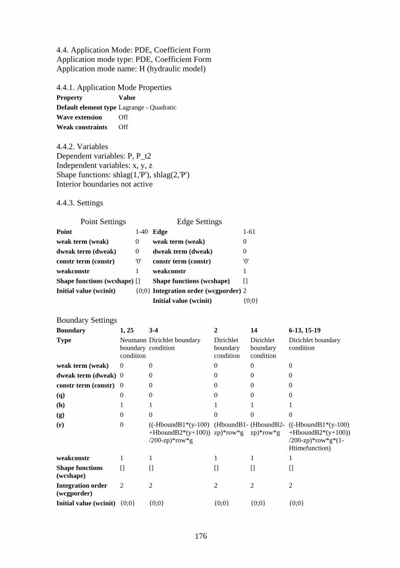
176

4.4. Application Mode: PDE, Coefficient Form Application mode type: PDE, Coefficient Form Application mode name: H (hydraulic model) 4.4.1. Application Mode Properties Property Value Default element type Lagrange - QuadraticWave extension Off Weak constraints Off 4.4.2. Variables Dependent variables: P, P_t2 Independent variables: x, y, z Shape functions: shlag(1,'P'), shlag(2,'P') Interior boundaries not active 4.4.3. Settings

Point Settings Edge Settings Point 1-40 Edge 1-61 weak term (weak) 0 weak term (weak) 0 dweak term (dweak) 0 dweak term (dweak) 0 constr term (constr) '0' constr term (constr) '0' weakconstr 1 weakconstr 1 Shape functions (wcshape) [] Shape funcInitial value (wcinit) 0;0 Integration or Initial value Boundary Settings Boundary 1, 25 3-4 Type Neumann

boundary condition

Dirichlet boundcondition

weak term (weak) 0 0 0 0 0 dweak term (dweak) 0 0 0 0 0 constr term (constr) 0 0 0 0 0 (q) 0 0 0 0 0 (h) 1 1 1 1 1 (g) 0 0 0 0 0 (r) 0 ((-HboundB1*(y-100)

+HboundB2*(y+100))/200-zp)*row*g

(HboundB1-zp)*row*g

(HboundB2-zp)*row*g

((-HboundB1*(y-100) +HboundB2*(y+100)) /200-zp)*row*g*(1-Htimefunction)

weakconstr 1 1 1 1 1 Shape functions (wcshape)

[] [] [] [] []

Integration order (wcgporder)

2 2 2 2 2

Initial value (wcinit) 0;0 0;0 0;0 0;0 0;0

ary Dirichlet boundary condition

Dirichlet boundary condition


tions (wcshape) [] der (wcgporder) 2

(wcinit) 0;0

2 14 6-13, 15-19

Subdomain Settings Subdomain 1, 3 Shape functions (shape) shlag(1,'T') shlag(1,'P') shlag(2,'u') shlag(2,'v') shlag(2,'w') Integration order (gporder) 2 Constraint order (cporder) 1 weak term (weak) 0 dweak term (dweak) u_test*(b1*ux_time+b6*uy_time+b5*uz_time)+

v_test*(b6*vx_time+b2*vy_time+b4*vz_time)+ w_test*(b5*wx_time+b4*wy_time+b3*wz_time)

constr term (constr) 0 Diffusion coefficient (c) 'k1/muw','k6/muw','k5/muw';

'k9/muw','k2/muw','k4/muw'; 'k8/muw','k7/muw','k3/muw'

Absorption coefficient (a) 0 Source term (f) (thetaeq*betaTw)*T_time Mass coefficient (da) 1/G Conservative flux convection coeff. (al) 0;0;0 Convection coefficient (be) 0;0;0 Conservative flux source term (ga) '-row*g*k5/muw';'-row*g*k4/muw';'-row*g*k3/muw' weakconstr 1 Subdomain initial value 1, 3 P ((-HboundB1*(y-100)+HboundB2*(y+100))/200-zp)*row*g 4.5. Application Mode: PDE, Coefficient Form Application mode type: PDE, Coefficient Form Application mode name: M (mechanic model) 4.5.1. Application Mode Properties Property Value Default element type Lagrange - QuadraticWave extension Off Weak constraints Off 4.5.2. Variables Dependent variables: u, v, w, u_t2, v_t2, w_t2 Independent variables: x, y, z Shape functions: shlag(2,'u'), shlag(2,'v'), shlag(2,'w') Interior boundaries not active 4.5.3. Settings

Point Settings Edge Settings Point 1-40 Edge 1-61 weak term (weak) 0;0;0 weak term (weak) 0;0;0 dweak term (dweak) 0;0;0 dweak term (dweak) 0;0;0 constr term (constr) '0';'0';'0' constr term (constr) '0';'0';'0' weakconstr 1 weakconstr 1 Shape functions (wcshape) [] Shape functions (wcshape) [] Initial value (wcinit) 0;0;0;0;0;0 Integration order (wcgporder) 2 Initial value (wcinit) 0;0;0;0;0;0

177

Boundary Settings Boundary 6-13, 15-19 4 1, 25 2, 14 3 Type Neumann

boundary condition

Neumann boundary condition




weak term (weak) 0;0;0 0;0;0 0;0;0 0;0;0 0;0;0 dweak term (dweak) 0;0;0 0;0;0 0;0;0 0;0;0 0;0;0 constr term (constr) '0';'0';'0' '0';'0';'0' '0';'0';'0' '0';'0';'0' '0';'0';'0' (q) 0,0,0;0,0,0;

0,0,0 0,0,0;0,0,0;0,0,0 0,0,0;0,0,0;

0,0,0 0,0,0;0,0,0; 0,0,0

0,0,0;0,0,0; 0,0,0

(h) 1,0,0;0,1,0; 0,0,1

1,0,0;0,1,0;0,0,1 1,0,0;0,0,0; 0,0,0

0,0,0;0,1,0; 0,0,0

1,0,0;0,1,0; 0,0,1

(g) 0;0;0 0;0;'(400-35)*roeq*g* Mtimefunction'

0;0;0 0;0;0 0;0;0

(r) 0;0;0 0;0;0 0;0;0 0;0;0 0;0;0 weakconstr 1 1 1 1 1 Shape functions (wcshape)

[] [] [] [] []

Integration order (wcgporder)

2 2 2 2 2

Initial value (wcinit) 0;0;0;0;0;0 0;0;0;0;0;0 0;0;0;0;0;0 0;0;0;0;0;0 0;0;0;0;0;0 Subdomain Settings Subdomain 1, 3 Shape functions (shape) shlag(1,'T') shlag(1,'P') shlag(2,'u') shlag(2,'v') shlag(2,'w') Integration order (gporder) 2 2 2 Constraint order (cporder) 1 1 1 weak term (weak) 0;0;0 dweak term (dweak) 0;0;0 constr term (constr) '0';'0';'0' Diffusion coefficient (c) '-t11';'-t16';'-t66';'-t15';'-t56';'-t55','-t16','-t12','-t14';'-t66','-

t26','-t46';'-t56','-t25','-t45','-t15','-t14','-t13';'-t56','-t46','-t36';'-t55','-t45','-t35';'-t16','-t66','-t56';'-t12','-t26','-t25';'-t14','-t46','-t45','-t66';'-t26';'-t22';'-t46';'-t24';'-t44','-t56','-t46','-t36';'-t25','-t24','-t23';'-t45','-t44','-t34';'-t15','-t56','-t55';'-t14','-t46','-t45';'-t13','-t36','-t35','-t56','-t25','-t45';'-t46','-t24','-t44';'-t36','-t23','-t34','-t55';'-t45';'-t44';'-t35';'-t34';'-t33'

Absorption coefficient (a) 0,0,0;0,0,0;0,0,0 Source term (f) '(b1*Px+b6*Py+b5*Pz)+(betaTs*(t11+t12+t13)*Tx+betaTs*

(t16+t26+t36)*Ty+betaTs*(t15+t25+t35)*Tz)';'(b6*Px+b2*Py+b4*Pz)+(betaTs*(t16+t26+t36)*Tx+betaTs*(t12+t22+t23)*Ty+betaTs*(t14+t24+t34)*Tz)';'roeq*g+(b5*Px+b4*Py+b3*Pz)+(betaTs*(t15+t25+t35)*Tx+betaTs*(t14+t24+t34)*Ty+betaTs*(t13+t23+t33)*Tz)'

Mass coefficient (da) 0,0,0;0,0,0;0,0,0 Conservative flux convection coeff. (al) 0;0;0,0;0;0,0;0;0;0;0;0,0;0;0,0;0;0;0;0;0,

0;0;0,0;0;0 Convection coefficient (be) 0;0;0,0;0;0,0;0;0;0;0;0,0;0;0,0;0;0;0;0;0,

0;0;0,0;0;0 Conservative flux source term (ga) 0;0;0;0;0;0;0;0;0 weakconstr 1

178

Subdomain initial value 1, 3 u 0 v 0 w 0 5. SOLVER SETTINGS Solve using a script: off Auto select solver on Solver Time dependent Solution form weak Symmetric off Adaption off 5.1. Direct (UMFPACK) Solver type: Linear system solver Parameter Value Pivot threshold 0.1 Memory allocation factor 0.7 5.2. Time Stepping Parameter Value Times Linspace(0,1e8,100)Relative tolerance 0.01 Absolute tolerance 0.0010 Times to store in output Tsteps Time steps taken by solver Free Manual tuning of step size Off Initial time step 0.0010 Maximum time step 1.0 Maximum BDF order 5 Singular mass matrix Maybe Consistent initialization of DAE systems 2 Error estimation strategy 0 Allow complex numbers Off 5.3. Advanced Parameter Value Constraint handling method EliminateNull-space function Auto Assembly block size 5000 Use Hermitian transpose On Use complex functions with real input Off Type of scaling Auto Manual scaling Row equilibration On Manual control of reassembly Off Load constant On Constraint constant On

179

APPENDIX XIII: Full article of the reference [22] (Preprint)

This APPENDIX contains a fac-simil of the article labelled in the list of

references as [22], which corresponds to the time series analysis performed in the Chapter 3 of the thesis. The complete reference of this article is again given here:

Cañamón, I., Elorza, F.J., Mangin, A., Martín, P.L. & Rodríguez, R. Wavelets

and Statistical Techniques for Data Analysis in a Mock-Up High-Level Waste Storage Experiment. International Journal on Wavelets, Multiresolution & Image Processing 2(4): pp. 351-370. December 2004.

181

APPENDIX XIV: Full article of the reference [3] (Preprint) This APPENDIX contains a fac-simil of the article labelled in the list of

references as [3], which corresponds to the dual-continuum model described in APPENDIX VI as an alternative for the hydraulic part of the T-H-M model of the Chapter 6 of the thesis. The complete reference of this article is again given here:

Ababou, R, Cañamón, I., Elorza, F.J. Thermo-Hydro-Mechanical Simulation of

a 3D Fractured Porous Rock: Preliminary Study of Coupled Matrix-Fracture Hydraulics. Proceedings of the COMSOL Multiphysics Conference 2005, pp. 193-198. Ed. J. M: Petit and J. Daluz. France. November 2005.

203

Abstract We present a problem involving the modeling of coupled flow and elastic strain in a 3D fractured porous rock, which requires prior homogenization (upscaling) of the fractured medium into an equivalent darcian anisotropic continuum. The governing equations form a system of PDE’s (Partial Differential Equations) and, depending on the case being considered, this system may involve two different types of “couplings” (in a real system, both couplings (1) and (2) generally take place):

1) Hydraulic coupling in a single (no exchange) or in a dual matrix-fracture continuum (exchange);

2) Thermo-Hydro-Mechanical interactions between fluid flow, pressure, elastic stress, strain, and temperature (after Ababou et al. 1994 [1]).

We present here a preliminary model and simulation results with FEMLAB®, for the hydraulic problem with anisotropic heterogeneous coefficients. The model is based on data collected at an instrumented granitic site (FEBEX project) for studying a hypothetical nuclear waste repository at the Grimsel Test Site in the Swiss Alps.

Keywords: FEMLAB. Numerics. Porous

fractured media. Coupled PDE systems. Darcy’s law. Permeability upscaling. Dual continuum. Fluid exchange. Biot. Hydro-mechanics. Poro-elasticity.

1 Introduction

This article presents a preliminary study of fractured rock, including fracture network reconstruction and numerical flow simulations, as a first step towards a fully coupled Thermo-Hydro-Mechanical (T-H-M) analysis of a fractured granite formation located at the Grimsel Test Site (GTS, Switzerland), where the FEBEX experiment is located. FEBEX is an experiment to test the T-H-M behavior of a crystalline high-level waste repository.

The aim of the preliminary simulations presented below is to reproduce the hydraulic behavior of the fractured medium using either single or dual continuum approaches to the fractured porous rock. The macroscale continuum equations and coefficients are obtained by upscaling from the local Darcy

equation (matrix) and Poiseuille-type equation (fractures) up to block scale, where each homogenized block contains ideally many fractures. But, to obtain the upscaled equations requires knowledge of the morphology of the 3D fracture network. The overall procedure can be summarized as follows. First, the 3D network is obtained by a statistical

reconstruction method (or inversion method) based on various fracture statistics and on detailed observations of fracture traces on tunnel drifts and boreholes.

Secondly, the domain of interest is partitioned into sub-domains, in which the fractured rock is represented as a set of single-fractured ‘blocks’. The tensorial upscaled coefficients are computed at the scale of the sub-domains based on superposition approximations.

Thirdly, the corresponding system of continuum PDE’s are solved numerically for initial-boundary conditions, with a numerical mesh finer than block scale, using (here) 3D finite element PDE solvers in FEMLAB® [3].

In this preliminary paper, only the hydraulic upscaling will be applied. A set of 3D numerical experiments with either single or dual continuum equations will be presented. For this reason, the upscaling of hydraulic coefficients is briefly presented. The hydraulic simulations are performed using the FEMLAB® multiphysics software. Although the full THM model is not implemented here, the principles of coupled hydro-mechanics are still briefly explained. The THM model yields a tensorial non-orthotropic (rank 4) PDE system to be solved with FEMLAB® multiphysics. 2 Characterization of the 3D fractured medium (network) 2.1 Experimental site: geology, fracture data GEOLOGY, TUNNEL, BOREHOLES.

The GTS is located in the southern part of the Central Aar Massif, around 400m below the surface. The rocks in this area are mostly granitic, and are

Rachid ABABOU, Israel CAÑAMÓN, Fco. Javier ELORZA

Thermo-Hydro-Mechanical simulation of a 3D fractured porous rock: preliminary study of coupled matrix-fracture hydraulics.

204

-1

-0,8

-0,6

-0,4

-0,2

0

0,2

0,4

0,6

0,8

1

-1 -0,8

-0,6

-0,4

-0,2

0 0,2 0,4 0,6 0,8 1


3

1 2

4

intruded by lamprophyres and aplites. The FEBEX experiment is located in the northern part of the GTS Laboratory tunnel, where a marked water discharge was encountered. Two exploratory boreholes where made: FEBEX-95001 and -95002.

FRACTURE NETWORK STRUCTURE (DATA)

A general lithologic and structural cartography of the gallery was developed (Figure 1), where five different zones were distinguished along the main axis of the gallery:

Figure 2: Fracture orientation data coming from boreholes FEBEX-95001 and FEBEX-95002 : pole diagram with 5 families.

OPTIMIZATION/RECONSTRUCTION ALGORITHM

An optimization procedure, based on simulated annealing, was used to adjust fracture size distribution so as to minimize (via an appropriate error norm criterion) the discrepancy between the frequency histograms of observed and simulated tunnel traces. The criterion also takes into account the observed vs. simulated discrepancy of the number of fracture intersections with the exploratory boreholes and the tunnel. The main features of the fracture system where imposed in order to preserve the model’s geometric and hydraulic consistency given other sources of information (major geologic structures, observed tunnel seepages, etc). Here, we only show a preliminary example of the optimally reconstructed 3D fracture network. The optimization algorithm will be detailed in another paper.

Figure 3 shows the reconstructed 3D fracture network, which has N = 18 272 disc fractures. The 3D generation domain consists of a block of 70mx100mx70m (a volume of 490 000 m3) centered on the FEBEX gallery. The negative X axis points towards the Geographic North (South-North axis).

Figure 3: Reconstructed fractured network.

XYZ

Figure 1: Map of traces on the wall of the FEBEX gallery, divided into five different zones [8].

For example, the 2nd tunnel zone (x=14.0-25.5 m) has high fracture density: there are some breccified zones (breccias) with more than 10 fractures/m; the granite is highly altered in this zone, and water flow is approximately 70 l/day overall. A pole plot of the fracture orientations and their partition into 5 sets (families) was established according to the GTS geologic studies [6, 9]. The distribution of fractures along the two exploratory boreholes is available [not show here for lack of space].

2.3. Statistical network generation : inverse problem, optimization, reconstruction

A synthetic fractured medium was generated from the field data, i.e., reconstructed statistically based on field data. First, the following fracture parameters and statistics were defined (and if possible pre evaluated) by using the above-described geologic information:

- Fracture positions. Homogeneous Poisson process for the (x,y,z) coordinates of fracture centers.

- Fracture orientations. Four different families of fractures were defined according to both morphological (stereonet) and genetic criteria. Uniform distributions for the direction and the plunge were used. Figure 2 shows the pole diagram.

- Fracture densities. One of the densities used in the calibration process is the density ρ21 of tunnel traces (trace length / intersecting plane area).

- Fracture aperture. Data on fracture aperture are only qualitative. Distinguishing ‘filled’, ‘open’ and ‘wet’ fractures, leads to assigning a priori apertures of 1E-8m, 1E-5m and 1E-2m respectively.

- Fracture size. A power law distribution was used for fracture diameters or radii. The parameters of this distribution (RMIN, RMAX, b exponent) were optimized so that the synthetic network fits the geologic data.

205

206

3 Hydraulic model for fractured porous media: upscaling, equations 3.1. Single and dual continuum flow equations SINGLE MEDIUM : MATRIX-FRACTURE CONTINUUM FLOW EQUATION.

The governing equation for the upscaled single continuum is of the same form as the classical Darcy equation for incompressible single phase flow (where the upscaled permeability must be considered a 2nd rank tensor, as will be seen):

⎟⎠⎞

⎜⎝⎛ ∇∇=

∂

∂P

tP

.Kµ

θ 1.C

DUAL CONTINUUM MATRIX-FRACTURE FLOW SYSTEM. The governing equations for the upscaled dual

continuum model are a coupled system of two equations (generalizing the “dual porosity” model initially developed by [2]):

( )

( )⎪⎪⎩

⎪⎪⎨

⎧

−+⎟⎠⎞

⎜⎝⎛ ∇∇=

∂

∂

−−⎟⎠⎞

⎜⎝⎛ ∇∇=

∂∂

fmffff

f

fmmmmm

m

PPPt

P

PPPt

P

µα

µθφ

µα

µθφ

.K

.K

1.C

1.C

ff

mm

where : Pm is pressure in the “matrix” medium [Pa] Pf is pressure in the « fractures » medium [Pa] Kmm=KM is the equivalent upscaled permeability

tensor of the “matrix” medium [m2] Kff=KF is the equivalent upscaled permeability

tensor of the “fractures” medium [m2] µ is the dynamic viscosity of the fluid [Pa.s] (µ is

the ratio of a stress τ / grad V) α is the exchange coefficient between “matrix”

and “fractures” [Dimensionless] φm is the volumetric fraction of the “matrix”

medium per unit volume of space [m3/m3] φf is the volumetric fraction of the “fractures”

medium per unit volume of space [m3/m3] θm is the intrinsic porosity of the matrix [m3/m3] θf is the intrinsic porosity of the “fractures”

medium [m3/m3] Cm is the specific elastic storage coefficient of the

“matrix” continuum [Pa-1] Cf is the specific elastic storage coefficient of the

“fractures” continuum [Pa-1] Note that we have distinguished here volume

fractions from porosities, and we have introduced a “fracture porosity” θf, even though θf = 1 usually for a clean rock joint. However we also consider the case of deposit-filled fractures, faults, disturbed zones, and other geologic bodies such as lamprophyres: in all such cases we may specify θf < 1.

The pressures “P” [Pa] in the matrix and fractures are phase-averaged over the upscaled unit volume or block. The intrinsic permeabilities “K” [m2] are the equivalent upscaled permeabilities for each continuum, defined over the same scales as pressure. They are taken here to be positive second rank tensors (as will be seen).

The coefficients “C” [Pa-1] are specific storage coefficients, or “capacities”. They express the capacity to store or drain a m3 of fluid per m3 of medium due to a unit variation of pressure. Since the medium is saturated (single phase flow) this capacity is due solely to compressibility effects. Thus, it is assumed that the fluid and the two continuous media (matrix, fractures) all react like elastic isotropic continua to changes of pressure. It is possible to rewrite the above equations using a new set of elastic capacities “c” [s]: mmCθµφmmc = ; ff Cθµφ ffc =

where lower case capacities “c” are in units of time [s], while upper case capacities “C” are in inverse pressure units [Pa-1]. The system can now be expressed in terms of (cm,cf) as follows:

( ) ( )

( ) ( )⎪⎪⎩

⎪⎪⎨

⎧

−+∇∇=∂

∂

−−∇∇=∂

∂

fmffff

f

fmmmmm

m

PPPt

Pc

PPPt

Pc

α

α

.K

.K

.

.

PURE EXCHANGE DUAL CONTINUUM EQUATIONS. To obtain a pure exchange process with negligible

pressure gradient terms, let us assume that the matrix is only weakly conductive compared to the fracture network, that is: KM << KF or, perhaps more accurately: φm KM << φf KF. This allows us to neglect the pressure gradient terms ("transport" terms) in the matrix flow equation (∂Pm/∂t) above. In addition, we assume that, since the fracture medium permeability is comparatively high, the pressure gradient in the "fracture continuum" is negligible in each upscaling domain. This allows us to neglect the pressure gradient terms in the “fractures” medium (equation ∂Pf/∂t). If we also neglect, for simplicity, the spatial fluctuations of (φ, θ, C) in each medium, we can show that the pressure difference is governed by a purely kinetic equation (“pure exchange”) :

Pt

P ~C

~

µα

−=∂

∂ where 2

~ fm PPP

−= .

This equation was used by Kfoury, Ababou et al (2004) to analyze the second upscaling problem, where the local α (at the scale of unit cell) is randomly heterogeneous, and the upscaling of α is sought on a larger scale comprising many unit cells.

3.2. Single medium hydraulic upscaling

In this section, we develop the macroscale Darcy flux equations at the scale of a homogenization sub-domain, possibly containing many fractures or ‘fracture blocks’ (as explained in the following). The upscaling approach being used will only be outlined here. It is essentially based on a flux superposition principle similar to that used in the thermo-hydro-mechanical upscaling equations developed in [1] and [9] for the case of a fractured rock with impervious

porous matrix. The fact that matrix permeability is no longer neglected here, constitutes a generalization of the above-cited works.

The region of interest is partitioned into sub-domains, in which the flow equation must be homogenized. Most importantly, in each sub-domain, the 3D medium is idealized as an assembly of blocks, each block being constituted of the porous matrix traversed by a single planar fracture. Let us now express some intermediate steps and give the final result.

First, we express as follows the microscale tensorial conductivities characterizing the local head loss law within each medium (single fracture and its surrounding matrix) composing a “block”: Isotropic porous matrix (M):

Anisotropic fracture, or fault, or coarse medium (F):

where:

is conductivity parallel to fracture, e.g. Poiseuille law (for a ‘real’ fracture)

is conductivity transverse to fracture, e.g. quasi-infinite (real fracture)

IK M

M

M

M

M KK

KK

=⎟⎟⎟

⎠

⎞

⎜⎜⎜

⎝

⎛=

000000

⎟⎟⎟

⎠

⎞

⎜⎜⎜

⎝

⎛

=⊥F

F

F

F

KK

K

000000

||

||

K

||FK

⊥FK

Secondly, the exact equivalent conductivity for the

single-fracture block of Figure 4 is calculated, according to the ‘low order’ upscaling approach evoked earlier. The result is:

( ) ( ) HjiAjiijij KnnKnn ⋅+⋅−=

ΩδK

where KA is the arithmetic mean of (KF , KM ), and KH is their harmonic mean. Both are weighted by the corresponding volumetric fractions of ‘F’ and ‘M’ at block scale [ϕ and (1-ϕ) respectively]. Also, ni is the ith-component of the unit vector normal to fracture.

Finally, we define the geometry of individual fracture blocks. One approach is to let each block be a prismatic volume having same cross-section as the corresponding planar fracture. Thus, if the fracture is a disc, the block is a circular cylinder; if the fracture is rectangular, the block is a parallelepipedic box. The heights (bk) of the blocks (k=1,2…) can be chosen constant (bk =b) within the homogenization domain, such that the cumulated volume of all blocks (Vk) equals the volume of the domain (V ):

Ψ

bS

VbFN

mm

k ==

∑=

Ψ

1

b/2

b/2

a

x

z

l

l

ΓI

ΓF Ω

ΩA

ΩC

ΩB

zHJ z ∂

∂−=

xHJ x ∂

∂−=

ΩC

ΩB

ΩA

Figure 4: Basic building block of a fractured porous medium, showing Boundary Conditions with imposed piecewise linear hydraulic head H (total pressure P).

Finally, a flux superposition approach is applied over all the individual blocks. Several alternative approaches are considered, including: (i) volume-weighted average of block-scale Darcy flux density vector q [m/s]; and (ii) direct sum of block-scale fluxes Q [m3/s]. The latter approach just adds up the individual block contributions to the global flux:

∑=k

kQQ

which requires a prior estimate of the individual block flux Qk. But only the flux density qk is known, since the earlier block-upscaling step yields a block-scale Darcy equation in terms of flux density. Therefore, to obtain the block flux Qk requires a prior estimate of the effective cross-sectional flux area of the block. Dividing the flux Qk by the total cross-sectional area (AT) of the homogenization domain, yields finally Darcy’s law in terms of Darcy velocity (flux density). This yields finally the equivalent conductivity tensor :

( )( ) ( )( ) ( )( ) ( )( )∑

⎢⎢⎢⎢⎢

⎣

⎡

+⋅+⋅−⋅−Α

Α=

kF

kM

kkj

kiij

T

k

ij KKnnK ϕϕδ ...1 ||

( ) ( )( )( ) ( )

⎥⎥⎥⎥⎥

⎦

⎤

+−

⋅+

⊥F

k

M

kk

jk

i

KK

nnϕϕ1

1

This Kij tensor gives the mean response of the fractured porous medium to a given global gradient.

3.3. Dual medium model : exchange coefficient (and permeabilities)

The upscaling approach developed for a single matrix/fracture medium, can also be used for upscaling, separately, the matrix and fracture system permeabilities in the dual medium equations: UPSCALED PERMEABILITY OF THE 1RST MEDIUM – THE POROUS MATRIX. Assuming the porous matrix composing the intact rock to be homogeneous and isotropic, the upscaled matrix permeability tensor is simply the local scalar permeability, that is:

Ψ

=

⋅=

∑V

S

SVFN

mm

kk

1 . δMM KK =ˆ

207

UPSCALED PERMEABILITY OF THE 2ND MEDIUM – THE FRACTURE SYSTEM. To upscale separately the fracture network, constituting the 2nd medium, we may re-use the previous matrix-fracture upscaling, simply by inserting KM=0 there. The result is a fracture permeability tensor of the form:

( )( )

( ) ( )( ) ( )[ ]∑ ⋅−Α

Α=

kF

kkj

kiij

T

k

ijF KnnK ||ˆ ϕδ

UPSCALED MATRIX/FRACTURE EXCHANGE – THE SCALAR EXCHANGE COEFFICIENT α. The exchange coefficient needs to be evaluated at subdomain scale (homogenization scale). The upscaled α proposed in this paper is an extension from the original Warren-Root formula [10]. More recent studies [5] confirm, to some degree, the Warren-Root intuition, at least for a regular or periodic array of fractured blocks. Following in part [5], we propose to evaluate the dimensionless α coefficient at sub-domain scale as:

( ) 22

λπα

K= ; ( ) MFM KKKK ≈⎥⎦

⎤⎢⎣⎡ +=

−−−

111

21

and the characteristic length scale λ is the effective interspacing distance between fracture planes. We evaluate it from the specific area density ρ32 defined in the FRACMAN code [4], following also [1]:

321

ρλ ≈ .

4 Implementation of coupled hydraulics: the FEMLAB® model

The domain of investigation is a fractured rock block of 70mx100mx70m that contains the FEBEX tunnel. The X-axis points to the North, and the FEBEX tunnel has an orientation of N-270-E. The origin of the domain is located at the center of the fractured block, and coincides with the center of the tunnel. A regional flow parallel to +X is considered.

Three measurement points, or probes, are defined for output purposes: (i) the lamprophyre dyke sample point; (ii) the tunnel sample line (right wall of tunnel); (iii) the flow sample line (along X-axis). Figure 5 and Table 1 show the main features of the domain and the mesh used in FEMLAB’s 3D finite element model.

Figure 5: The 70mx100mx70m region of interest showing the model’s measuring points (probes).

# of elements

# of nodes

# of boundary elements

# of edge elements

8315 24798 1294 110 Table 1: The 3D Finite Element Mesh.

5 Flow simulation results and discussion Several flow experiments have been modeled.

Each of them focuses on a different aspect of the hydraulic model. The experiments are divided in: Pure exchange experiments: The initial-

boundary conditions are such that there is no net flow at the scale of the domain. Only matrix-fracture exchange takes place, controlled by coefficient α estimated from the synthetic fractured network (see final equation of section 3.3). Two different ‘pure exchange’ experiments were carried out: (I.1) homogeneous α; (I.2) heterogeneous α on a 3x3x3 partition.

Flow-through experiments: In this set of experiments, the boundary conditions are such that there exists a mean flux, and a non zero pressure gradient, across the entire domain (‘flow-through’ experiments). Several numerical experiments were conducted, some coinciding with the full dual medium model, others reducing to the single medium without exchange (all with partitions of 3x3x3): . (II.1) Single medium / no exchange; (II.2.1) Dual medium / low flow regime; (II.2.2) Dual medium, negligible exchange; (II.2.3) Dual medium with both flow+exchange.

Figure 6a. shows the spatial distribution of the estimated α for the fractured medium. It is represented as spheres of radius proportional to α, one for each of the subdomains in the 3x3x3 partition. Figure 6b. shows ellipsoids of Keq for each partition. This value of Keq has been computed for a matrix conductivity KM=0, and is the one used for the dual medium model, whereas in the single medium mode we compute Keq using a value for KM=1e-12m2. In all the experiments, the final simulation time was sufficiently large to reach steady state. In most cases, this final time was around T=1E+11 s ≈ 3000years. In this paper we only show the results of the experiment (II.2.1).

a. Exchange coefficient α.

b. Equivalent hydraulic conductivity Keq.

Figure 6: 3D distribution of the model parameters represented in the centers of the partition blocks.

Right wall sample line

Flow direction sample line

Lamprophyre sample point

208

209

EXPERIMENT II.2.1: DUAL-MEDIUM HYDRAULICS WITH LOW FLOW REGIME

In this experiment the pressure Pf(t) in the fracture medium decreases quickly during the early stages of the experiment. However, steady state flow is reached later than in the single medium experiment. This is because the upscaled permeability of the single medium combines matrix and fracture, whereas it only considers the ‘fracture’ medium permeability in this experiment.

The evolution can be divided in two stages: in the first stage (early times) we get similar results than those found for the pure exchange experiment (I.2) (Figure 7), and in the second stage (late times) we obtain the same behavior as that observed for the single medium ‘flow-through’ experiment (II.1) (Figure 8).

In this case, after the exchange equilibrium is reached, both fracture and matrix media behave exactly the same in the flow transitory. This means that, in the latest stages, this model behaves completely equivalent to the single medium model.

Figure 7: Distribution of Pf at time T=1e+6s (≈12 days) at measuring points (probes), for the dual medium ‘flow-through’ experiment with low flow regime.

Figure 8: Distribution of Pf at time T=1e+11s (≈3000 years) at measuring points (probes) for the dual medium ‘flow-through’ experiment with low flow regime.

6. Conclusions and future work

We presented here a preliminary model and simulation results with FEMLAB®, for the hydraulic problem with anisotropic heterogeneous coefficients.

The model is based on data collected at an instrumented granitic site (FEBEX project) for studying a hypothetical nuclear waste repository at the Grimsel Test Site in the Swiss Alps. This approach allows us to quantify the influence of a 3D fracture network on the hydraulics of fractured rocks.

In this paper, thermo-hydro-mechanical (T-H-M) coupling is not implemented. However, the aim of this work in the future is to fully implement hydro-mechanical coupling (and thermal stresses as well). This will be done, in a first step, by considering the fractured rock as a single equivalent poro-elastic continuum. The reader is referred to the T-H-M upscaling theory developed in [1] and also reported in [9], for an impervious matrix. This theory will be extended to the case of a permeable porous matrix (Km≠0).

7. Acknowledgements

This work has been partially supported by the FEBEX project under contract number FIKW-CT-2000-0016 with the European Commission and ENRESA. References 1. Ababou R., A. Millard, E. Treille, M. Durin, and F.

Plas : Continuum Modeling of Coupled Thermo-Hydro-Mechanical Processes in Fractured Rock. Comput. Methods in Water Resources, Kluwer Academic Publishers, A. Peters et al. eds. Vol.1, Ch.6, pp.651-658 (1994).

2. Barenblatt G. , Zelthov I., Kochina I. Basic concepts in the theory of seepage of homogeneous liquids in fissured rocks. J. Appl. Math. 24 (1960), 213-240.

3. COMSOL, 2004: FEMLAB User’s Guide 3.1. COMSOL AB. October 2004. 581 pp.

4. Dershowtiz W. et al. (1992): FRACMAN v.2.3 : Interactive discrete feature data analysis, geometric modelling, and exploration simulation – User Doc. Redmond WA: Golder Assoc. 1992.

5. Dykhuisen, R.C. (1990). A new coupling term for dual-porosity models. Water Resour. Res., 1990, 26(2):351-356.

6. Keusen, H.R., Ganguin, J., Schuler, P., Buletti, M. (1989): Grimsel Test Site: Geology. NAGRA Tech. Report. NTR 87-14E. (Ref [6])

7. Kfoury M., R. Ababou, B. Noetinger and M. Quintard, 2004. Matrix-fracture exchange in fractured porous media: stochastic upscaling. Comptes-Rendus Académie Sciences (Paris). C.R. Mecanique, 2004, Vol.332, pp.679-686.

8. Pardillo J., Campos R., Guimerá J. (1997): Caracterización geológica de la zona de ensayo FEBEX(Grimsel-Suiza). CIEMAT-IMA-M-2-01.

9. Stietel A., Millard A., Treille E., Vuillod E., Thoraval A., Ababou R.: Continuum Representation of Coupled Hydro-Mechanical Processes of Fractured Media: Homogenisation and Parameter Identification. In : ‘Devts. Geotech. Engg.’: Coupled Thermo-Hydro-Mecha. Processes (DECOVALEX). O.Stephansson, L.Jing, C-F.Tsang eds. 79:135-164, Elsevier (1996).

10. Warren J.E. and P.J. Root (1963). The behavior of naturally fractured reservoirs. Soc. Petrol. Eng. J., 3(5), 245-255, 1963.

APPENDIX XV: Full article of the reference [23] (Preprint)

This APPENDIX contains a fac-simil of the article labelled in the list of references as [23], which corresponds to the simulation of the three-dimensional fractured network described in Chapter 4 of the thesis. The complete reference of this article is again given here:

Cañamón, I., Elorza, F. J., Ababou, R. 3D Fracture Networks: Optimal Identification and Reconstruction. Accepted for publication in the proceedings of the XIth IAMG Annual Congress. Belgium. September 2006.

211

International Association of Mathematical Geology XIth International Congress,

Université de Liège - Belgium

3D Fracture Networks: Optimal Identification and Reconstruction.

I. Cañamón1, F. J. Elorza1, R. Ababou2

1 Departamento de Matemática Aplicada y Métodos Informáticos, E.T.S.I. Minas, Universidad Politécnica de Madrid, Spain

2 Institut de Mécanique des Fluides de Toulouse, Institut National Polytechnique de Toulouse, France

Corresponding author: [email protected] ABSTRACT : In this paper we generate a 3D fractured medium that reproduces the non-uniform map of

fracture traces left on the wall of a cylindrical gallery. A specific algorithm calculating the analytic intersection of the fractures with the gallery has been developed, and appropriate statistical measures to compare both real and simulated media have been defined. In addition, other geological data such as orientations and fracture densities have been used, and size distribution parameters have been determined in the optimization procedure to best fit the tracemap in a real case study. Satisfactory concordance between measured and generated fractured media maps of traces is reached.

KEYWORDS : 3D fractured medium, Montecarlo, cylindrical wall tracemap, inverse problem, reconstruction, non-uniform tracemap.

1. Introduction

Works on fractured media reconstruction generally take trace data from flat or pseudo-flat walls coming from the vertical parts of arc galleries (Gillespie 1993, La Pointe 2002), but there are a lot of cylindrical galleries whose tracemaps cannot be used by considering there walls as flat. We could approximate the cylinders as a set of elongated planes parallel to the axis of the gallery, but then long traces get cut through the several planes, so that tracelength is underestimated and reconstruction cannot be realistic in 3D. In this paper we describe a methodology to use the traces left on cylindrical galleries without plane approximations. To do that, analytical solution of the intersection in 3D of a disk-shaped fracture with a cylinder has been obtained. Then, some statistics have been defined to characterize the tracemap to be reproduced. Finally, a Montecarlo optimization procedure based on a variation of Simulated Annealing (Metropolis 1953, Goffe 1994) has been used to find the parameters of the fracture size distribution that best fits the tracemap. Additionally, a specific algorithm to reproduce the non-homogeneous trace density along the tracemap has been defined. The granitic medium reconstructed in this paper is located at the Grimsel Test Site (Switzerland) in the southern part of the Central Aar Massif, around 400m below the surface. The cylindrical gallery from which fracture trace data have been collected corresponds to the FEBEX experiment, and has been excavated in the northern part of the Laboratory tunnel of the GTS.

212



2. Fractured network data

Different discontinuity systems have been described within the Central Aar Masif: ductile systems (S1, S2 and S3), brittle systems (S4/K4, K2/L=lamprophyre direction, K1, K3 and S5) and tensile systems (ZK1 and ZK2). For a detailed description of the fracture systems present in the GTS see (Steck 1968, Keusen et al. 1989). According to this classification, genetically and morphologically similar fractured systems have been grouped and four fracture families have been identified. The statistical orientation distributions of these families have been obtained with the data coming from two exploratory boreholes near the FEBEX gallery (Pardillo et al. 1997) (see Figure 1).

-1

-0,8

-0,6

-0,4

-0,2

0

0,2

0,4

0,6

0,8

1

-1 -0,8

-0,6

-0,4

-0,2

0 0,2 0,4 0,6 0,8 1


3

1 2

4

12

Fig. 1. Pole diagram of the fractures intersecting boreholes FEBEX-95001 and FEBEX-95002 and regrouping into four fracture families.

The general cartography of fracture traces in the FEBEX gallery (Pardillo et al 1997) is presented in Figure 2, where the most important lithologic and structural features can be distinguished. Five different zones with different structural characteristics and trace density can be distinguished along the main axis of the gallery (see Figure 2). Tracemap of the FEBEX gallery has been digitalized and two types of measures have been obtained for identification purposes: - Linear density 21ρ : defined as the ratio between total trace length and the wall surface. It has been calculated for the five different zones. - Histograms: of the trace length and the 3D trace chord in the whole gallery, the last obtained by rebuilding the cylindrical gallery from the tracemaps and getting the 3D coordinates of the traces.

Fig. 2. Development of the cylindrical tracemap in the FEBEX gallery with the five different zones of

fracture intersection density. Zone 4 includes a lamprophyre dyke highly transmissive.

Zone 1 Zone 2 Zone 3 Zone 4 Zone 5

213



214

3. Methodology for the reconstruction of the fractured medium

The exact analytical solution of the intersection of a disk fracture with a cylindrical tunnel comes out from solving the following system of equations:

22,222 tt

tttt

LxLRzy ≤≤−=+ (1)

(2)

where the first equation represents the cylinder and the second one the fracture disks, both of them in their respective local coordinated systems. Rt is the tunnel radius, Lt is the tunnel length, Ri is the i-th fracture disk radius, and Ndisks is the number of fracture disks. The solution of this system of equations yields to the analytical equation defining the trace. We obtain the extremes of the trace by solving the second equation as equality. From all the fracture traces appearing in the FEBEX gallery tracemap, seventeen features have a complete or near-complete trace. These fractures are big, and some of them are opened, and therefore relevant for creating preferential pathways for the fluid flux through the rock. It is important to take into account this features for reconstruction purposes, in order to preserve some geometric and hydraulic consistency in the model. According to previous geological studies, these features are large regional fractures, so a radius R=100, sufficiently large for the fractures to traverse the whole domain, has been assigned to them. To obtain their direction and plunge from the fracture traces, the following geometric relations have been used:

disksiiii NizRzy ,...,2,10,222 =∀=≤+

⎟⎠⎞

⎜⎝⎛+=

mDarctan2

πθ (3)

( )⎟⎟⎠

⎞⎜⎜⎝

⎛⋅

=⎟⎠⎞

⎜⎝⎛=

θϕ

sinarctanarctan

lD

LD (4)

where D is the diameter of the FEBEX gallery, m is the arc distance between the intersections of the trace with a horizontal plane passing through the gallery axis, and l is the arc distance between the intersections of the trace with a vertical plane passing through the gallery axis. A homogeneous Poisson process is used to define the coordinates ( )fcfcfc zyx ,,

ly distributed random wever, the non-uniform pattern

roduced, so. Ba

of each fracture center. Accordingly, these three coordinates are uniformvariables within the bounds of the rectangular box domain. Hoof the traces in the gallery wall showed in Figure 2 has also been rep that the distribution of centres in the proximities of the gallery must also be non-uniform sically, fracture density 21ρ is recalculated during the generation of fractures, until it reaches the experimental density on each zone of the FEBEX gallery. Each fracture lying in a zone where the maximum 21ρ has already been reached will then be moved towards another different zone. A Montecarlo algorithm has been implemented to reconstruct the synthetic fractured medium. An optimization procedure based on simulated annealing has been used to adjust fracture size distribution so as to minimize the discrepancy between the statistical characteristics of the


Université de Liège - Belgium synthetic fractured medium and those of the real fractured medium, according to the geologic data available. In this work, the power law or ‘Pareto’ distribution has been used to characterize the size of the fracture network, and only the Rmin and b parameters have been optimized (Rmax has been set to 100m).

4. Results and discussion

The optimization procedure yields to the determination of the parameters of the power law size distribution that best fit the geologic data: Rmin=0.1985m, Rmax=100m (fixed), and b=3,3048. Table 1 lists the main characteristics of the fractured network in terms of number of fractures and intersections with the different measured objects and with the corresponding simulated objects. Figure 3 shows the tracemap of the FEBEX gallery resulting from the optimized fractured medium, and Figures 4 and 5 present two 3D views of the fractured medium within the generation domain, which consists of a block of 70x200x70m3 centered in the FEBEX gallery. The simulated 3D fracture network has N = 2906474 disc fractures.

Fracture density 21ρ # traces

# intersect. FBX-01

# intersect. FBX-02 zone1 zone2 zone3 zone4 zone5 global

Measured 614 155 410 1.493 1.154 2.096 0.796 2.083 3.077 Generated 800 144 234 1.498 1.201 2.012 0.824 2.084 3.084 Tab. 1. Number of intersections with the gallery and the exploratory boreholes and fracture density

in the five gallery zones of the real and simulated fractured media.

Fig. 3. Development of the cylindrical tracemap obtained as intersection of the 3D simulated fractured

medium with the FEBEX gallery.

Figure 4: Disks of the simulated fractured

medium. Figure 5: Simulated fractured medium inside

the domain.

A good agreement has been obtained between the observed features, i.e. number of traces in tunnel and boreholes, fracture density and tracemap, and the ones produced by the simulated fractured medium. The non-uniformity of the tracemap has been also coherently reproduced.

N

x y

z

y

z

N

215



216

Although satisfactory results have been obtained, here are some comments for future work: - The non-homogeneous fractured network simulated near the gallery could be assumed

to be the same in the overall domain, so the statistical functions producing the fractured medium would be extended everywhere. To do that, non-homogeneous Poisson processes should be used (Stoyan et al. 1987), and some kind of density measure must be defined for every point in the 3D space. The reduced second moment function (Hanisch & Stoyan 1983) of the tracemap could be used for this purpose.

- The objective function has a stochastic nature, because it depends on the generation of a fractured medium obtained with statistical distributions. This means that, for the same set of parameters Rmin, Rmax, and b, we can obtain different values of the objective function for each realization. Therefore, an average of the objective functions of several realizations should be used to obtain a more reliable value given a set of parameters. The number of realizations to use in that average has to be determined according to the confidence interval needed in the objective function.

- For a hydrological validation of the fractured medium, hydraulic and transport tests available in the site should be used, with hydraulically conditioned fractured networks.

5. Conclusions

We have developed a methodology to simulate a 3D fractured network that fits optimally a cylindrical tunnel tracemap. The optimization procedure searches for the best parameters of the size distribution to minimize the discrepancies between measured and simulated trace length and 3D trace chord histograms and number of intersections with the tunnel and two exploratory boreholes. A good agreement between both fractured mediums has been found in the results. This methodology provides a good starting point for the use of cylindrical tracemaps to simulate geological 3D fractured networks, and completes the classical use of flat wall tracemaps that is more extensively developed in the literature.

Acknowledgments: The authors of this article would like to thank the FEBEX II project (EC contract FIKW-CT-2000-00016) to have provided them the opportunity to accomplish this study and to have provided with the experimental data used on it.

REFERENCES Gillespie, P.A., Howard, C.B., Walsh, J.J., & Watterson, J., 1993. Measurement and characterization of spatial distributions of fractures. Tectonophysics (226): 112-141. Goffe, Ferrier and Rogers, 1994. Global Optimization of Statistical Functions with Simulated Annealing. Journal of Econometrics (60, 1/2): 65-100. Hanisch, K.H., Stoyan, D., 1983. Remarks on statistical inference and prediction for a hard-core clustering model. Math. Operationsf. Statist., ser. statist. (14): 559-567. Keusen, H.R., Ganguin, J., Schuler, P., Buletti, M., 1989. Grimsel Test Site: Geology, Nagra Tech. Report, NTR 87-14E. La Pointe, P.R., 2002. Derivation of parent fracture population statistics from trace length measurements of fractal fracture populations. Int. Jour. Of Rock Mech. & Mining Sci. (39): 381-388. Metropolis, N., Rosenbluth, A., Rosenbluth, M., Teller A., and Teller, E. 1953. Equation of state calculations by fast computing machines. Jour. of Chem. Phys. (21): 1087–1092. Pardillo, J., Campos, R., Guimerá, J. , 1997. Caracterización geológica de la zona de ensayo FEBEX (Grimsel-Suiza). CIEMAT-IMA-M-2-01. Steck, A., 1968. Die alpidischen Strukturen in den zentralen Aare-Graniten des westlichen Aarmassivs. Eclogae geol. Helv. (61): 19-48. Stoyan, D., Kendall, W.S., Mecke, J., 1987. Stochastic Geometry and its Applications. J.Wiley&Sons.

ANALYSIS AND MODELING OF COUPLED THERMO-HYDRO

Documents

Transcript of ANALYSIS AND MODELING OF COUPLED THERMO-HYDRO