Hybrid hierarchical optical path network design algorithm with 2-stage ILP optimization
Upload
khangminh22Category
view
1download
0
Debora Botturi
An Optimization Approach toHybrid System Control
Ph.D. Thesis
31 Marzo 2005
Universita degli Studi di Verona
Dipartimento di Informatica

Advisor:prof. Paolo Fiorini
Series N: TD-01-05
Universita di VeronaDipartimento di InformaticaStrada le Grazie 15, 37134 VeronaItaly
i

Summary
The continuous growth of Minimally Invasive Surgery (MIS) operations is moti-vated by the apparently conflicting goals of better patient care and lower healthcare cost that MIS has been able to achieve. However, further increase in patientcare quality and cost reduction requires the development of new and more so-phisticated surgical techniques, with attention to the reduction of variability insurgical outcomes and to the increase of efficiency of MIS procedures. Towardsthis goal, many robotic devices were developed or proposed, and some of themare used in daily hospital practice. In the robotic assisted surgery, the proceduresare completely performed by the surgeon, and the robotic device is a mere, albeitsophisticated, tool. Thus, in order to keep increasing care quality and reducing itscost, it may be desirable and necessary to explore the development of algorithmsthat will endow a robotic assistant with the capability of collaborating with thesurgeon while performing MIS procedures. In this context, collaboration meansthat the robot is able to carry out certain small tasks autonomously, adapting tothe variability of the surgical arena, and with minimal guidance by the surgeon.This capability would reduce the strain on the surgeon, remove variability of sur-geons’ training levels and of procedure’s outcome, and enhance the overall systemefficiency by decreasing surgery time. In this Thesis we will examine the issuesrelated to the automatic execution of robotic tasks, in uncertain environmentssimilar to a surgical arena, and we will propose a method to compute the nominalcontrols for a robot that will carry out a typical surgical task.
Safety is the paramount problem in robotic surgery, and it will be even moreimportant in the automatic execution of surgical tasks. It is also well-known thatcurrent surgical robots lack force feedback, thus depriving the human operatorof a powerful way to control the robot performance. Thus, even now, a largeresponsibility for the correct task execution is put on the correctness of the controlalgorithms, because of the variability of the environment. In this Thesis, we pushthis concept further, by investigating safety using constraints on task execution,within an optimization approach. Variability is considered with respect to taskmodel and constraints, and is quantified as the distance of the current behaviorfrom the desired behavior of the robotic device during MIS. This approach allowsalso to continuously monitor task quality and operator performance.
iv
Traditionally, autonomous task execution has been approached by simplifyingthe problem using environment engineering, i.e. by adding suitable fixtures toremove task uncertainty. The most used advanced control technique consists of pre-programmed skills, so that different tasks can be programmed and executed usingthe same set of basic capabilities. When an explicit model of the environment is notavailable, skills are parameterized to allow for a certain degree of flexibility in thetask execution. If task and/or environment models are known or can be identified,it is possible to develop an explicit control law for the task execution. In this Thesiswe develop an explicit control law using the theory of Hybrid Systems, and wemodel uncertainty with appropriate sequences of states in the Hybrid System. Inparticular, we use deterministic automata as task model since the surgical gesturesstudied are well coded in the medical literature, and can be properly representedas autonomous tasks.
We represent a surgical task as a hybrid automaton, whose elementary staterepresents a distinct action of the task. In this way, we can compute the nominalcontrols by optimizing an appropriate quality index in the subtask domain, corre-sponding to each action of the task. In this context, the tradeoff between explicitmodel knowledge and feedback compensation strongly influences system perfor-mance. We investigate the relation between a priori knowledge, as representedby hybrid task automaton, the number and form of constraints, and the type ofon-line feedback to provide guidelines for the design of the complete system.
We argue that integration of techniques from hybrid system theory, constrainedoptimization and task constraint representation, help autonomy in uncertain envi-ronments. To demonstrate this, we simulate the autonomous execution of a suture,that is a common and very representative surgical gesture. The execution of thistask requires the definition of a nominal trajectory that can drive the robot to thetask successful completion. To this aim, we define an optimal strategy to computethe nominal control trajectory off-line and an on-line compensation of the devia-tion from the desired state trajectory. We conclude that the integration of differentmethods, such as hybrid systems, optimization methods, and optimal control con-tribute to the construction of safer autonomous executions of a realistic surgicaltask.
In summary, a set of tools for the synthesis of the control of a complex systemhas been proposed, investigated and evaluated in the context of autonomous surgi-cal tasks. The methods developed provide a rich basis for the treatment of complextask in unknown environments and expand on the state of the art of autonomoustask execution.
Acknowledgments
If I have seen further, it is by standing on the shoulders of giants.Isaac Newton
Paolo thanks to introduce me to the robotic field and to give me the freedomto pursue my own ideas, without you I would be a different kind of person in adifferent kind of world, thanks for your shoulders!Stefano thanks to be my friend, drawing for me and making the laboratory agood place to work.Andrea the matlab guy, thanks for your help! The discussions with you are alwaysvery stimulating.Markus you keep me down when flying is too dangerous! thanks to be myparachute when I decide to fly anyway!All my family grazie per aver capito cosa davvero conta per me.Dani my dear friend and example to follow, thanks for your advice.Lars stubborn guy, sofa and newspaper are waiting for you in my home!Vincent, Mark, Philippus lekker ding! I will never forget the philosophical mat-ter talk!Nicola pasta, wine and good company you can warm up your heart in a rainingday!Dado the singer, Puma has no secrets for him!Isabella perfect doctorate-mate, I was lucky to find you on my way.Biondo special summer schools mate, you know...I love Rome!Robotic community thanks to give me the feeling to be part of a big group andthe motivations to continue in this work, especially I want to thank Prof. HenrikChristensen to have hosted me at the very beginning, thank to the experience atCAS I decided to start the PhD, Prof. Stefano Stramigioli, thanks for your teach-ing and your enthusiasm, Prof. Maria Letizia Corradini, Prof. Roberto Segala,Prof. Maria Paola Bonacina and Prof. Bruno Siciliano thank you to be in my doc-torate committee.

Contents
1 Introduction . . . . . . . . . . . . . . . . . . . . . . . . . . . . . . . . . . . . . . . . . . . . . . . . . . . 11.1 The Challenge of Surgery Automatization . . . . . . . . . . . . . . . . . . . . . . 11.2 The Big Picture . . . . . . . . . . . . . . . . . . . . . . . . . . . . . . . . . . . . . . . . . . . . . 3
1.2.1 Teleoperation System . . . . . . . . . . . . . . . . . . . . . . . . . . . . . . . . . . 31.2.2 Surgical Systems . . . . . . . . . . . . . . . . . . . . . . . . . . . . . . . . . . . . . . 4
1.3 Thesis Objectives . . . . . . . . . . . . . . . . . . . . . . . . . . . . . . . . . . . . . . . . . . . . 51.4 Outline and Contributions . . . . . . . . . . . . . . . . . . . . . . . . . . . . . . . . . . . . 6
2 Autonomous Task Execution . . . . . . . . . . . . . . . . . . . . . . . . . . . . . . . . . . . 72.1 Definitions and General Concepts . . . . . . . . . . . . . . . . . . . . . . . . . . . . . . 72.2 Early Work in Autonomous Task Planning and Execution . . . . . . . . 112.3 Recent Work in Autonomous Task Planning and Execution . . . . . . . 12
2.3.1 Design, Sensing and Actuation Issues . . . . . . . . . . . . . . . . . . . . 122.3.2 Architectural Issues . . . . . . . . . . . . . . . . . . . . . . . . . . . . . . . . . . . . 15
2.4 Conclusions . . . . . . . . . . . . . . . . . . . . . . . . . . . . . . . . . . . . . . . . . . . . . . . . . 18
3 Hybrid System . . . . . . . . . . . . . . . . . . . . . . . . . . . . . . . . . . . . . . . . . . . . . . . . 193.1 Survey of systems and model . . . . . . . . . . . . . . . . . . . . . . . . . . . . . . . . . . 19
3.1.1 Classification of Dynamic Systems . . . . . . . . . . . . . . . . . . . . . . . 213.1.2 Discrete Event Systems . . . . . . . . . . . . . . . . . . . . . . . . . . . . . . . . 23
3.2 Hybrid Systems . . . . . . . . . . . . . . . . . . . . . . . . . . . . . . . . . . . . . . . . . . . . . 243.2.1 Modeling Approaches . . . . . . . . . . . . . . . . . . . . . . . . . . . . . . . . . . 26
3.3 Lyapunov Stability . . . . . . . . . . . . . . . . . . . . . . . . . . . . . . . . . . . . . . . . . . 313.3.1 Basic Definitions . . . . . . . . . . . . . . . . . . . . . . . . . . . . . . . . . . . . . . 333.3.2 Existing stability results . . . . . . . . . . . . . . . . . . . . . . . . . . . . . . . . 343.3.3 A Literature Review . . . . . . . . . . . . . . . . . . . . . . . . . . . . . . . . . . . 38
3.4 Conclusions . . . . . . . . . . . . . . . . . . . . . . . . . . . . . . . . . . . . . . . . . . . . . . . . . 42
4 Robotic Surgery . . . . . . . . . . . . . . . . . . . . . . . . . . . . . . . . . . . . . . . . . . . . . . . 434.1 Medical Aspects . . . . . . . . . . . . . . . . . . . . . . . . . . . . . . . . . . . . . . . . . . . . . 444.2 Clinical and Social Aspects . . . . . . . . . . . . . . . . . . . . . . . . . . . . . . . . . . . 474.3 Analysis and Segmentation of Surgical Task . . . . . . . . . . . . . . . . . . . . . 484.4 Suture . . . . . . . . . . . . . . . . . . . . . . . . . . . . . . . . . . . . . . . . . . . . . . . . . . . . . 50
VI Contents
4.4.1 Suture characteristics . . . . . . . . . . . . . . . . . . . . . . . . . . . . . . . . . . 504.4.2 Suture Model . . . . . . . . . . . . . . . . . . . . . . . . . . . . . . . . . . . . . . . . . 51
4.5 Conclusion . . . . . . . . . . . . . . . . . . . . . . . . . . . . . . . . . . . . . . . . . . . . . . . . . 53
5 Optimal Control Design . . . . . . . . . . . . . . . . . . . . . . . . . . . . . . . . . . . . . . . 555.1 Optimum System Control . . . . . . . . . . . . . . . . . . . . . . . . . . . . . . . . . . . . 55
5.1.1 Decision Processes . . . . . . . . . . . . . . . . . . . . . . . . . . . . . . . . . . . . . 575.1.2 Nominal Trajectory . . . . . . . . . . . . . . . . . . . . . . . . . . . . . . . . . . . . 58
5.2 Hybrid Optimal Control . . . . . . . . . . . . . . . . . . . . . . . . . . . . . . . . . . . . . . 625.3 Problem Formulation . . . . . . . . . . . . . . . . . . . . . . . . . . . . . . . . . . . . . . . . 645.4 Discussion and Conclusions . . . . . . . . . . . . . . . . . . . . . . . . . . . . . . . . . . . 66
6 Computational Issues . . . . . . . . . . . . . . . . . . . . . . . . . . . . . . . . . . . . . . . . . . 696.1 HOCP Solutions . . . . . . . . . . . . . . . . . . . . . . . . . . . . . . . . . . . . . . . . . . . . 69
6.1.1 Suboptimal Solution Technique . . . . . . . . . . . . . . . . . . . . . . . . . 706.1.2 Branch-and-Bound . . . . . . . . . . . . . . . . . . . . . . . . . . . . . . . . . . . . 71
6.2 TPBVP Solutions . . . . . . . . . . . . . . . . . . . . . . . . . . . . . . . . . . . . . . . . . . . 716.2.1 The Calculus of Variation and Optimal Control . . . . . . . . . . . 72
6.3 The Algorithm . . . . . . . . . . . . . . . . . . . . . . . . . . . . . . . . . . . . . . . . . . . . . . 746.4 Conclusions . . . . . . . . . . . . . . . . . . . . . . . . . . . . . . . . . . . . . . . . . . . . . . . . . 77
7 Computation Results and Simulations . . . . . . . . . . . . . . . . . . . . . . . . . 797.1 Introduction . . . . . . . . . . . . . . . . . . . . . . . . . . . . . . . . . . . . . . . . . . . . . . . . 797.2 Nominal Trajectory Computation . . . . . . . . . . . . . . . . . . . . . . . . . . . . . . 807.3 Simulation Results . . . . . . . . . . . . . . . . . . . . . . . . . . . . . . . . . . . . . . . . . . . 847.4 Conclusions . . . . . . . . . . . . . . . . . . . . . . . . . . . . . . . . . . . . . . . . . . . . . . . . . 85
8 Experimental Verification . . . . . . . . . . . . . . . . . . . . . . . . . . . . . . . . . . . . . . 878.1 The Experimental Setup . . . . . . . . . . . . . . . . . . . . . . . . . . . . . . . . . . . . . 878.2 Teleoperated Task Experiments . . . . . . . . . . . . . . . . . . . . . . . . . . . . . . . 908.3 Autonomous Task Experiments . . . . . . . . . . . . . . . . . . . . . . . . . . . . . . . 908.4 Conclusions . . . . . . . . . . . . . . . . . . . . . . . . . . . . . . . . . . . . . . . . . . . . . . . . . 93
9 Summary and Recomandation for Future Research . . . . . . . . . . . . 959.1 Contributions . . . . . . . . . . . . . . . . . . . . . . . . . . . . . . . . . . . . . . . . . . . . . . . 969.2 Recommendations for Future Research . . . . . . . . . . . . . . . . . . . . . . . . . 969.3 Conclusion . . . . . . . . . . . . . . . . . . . . . . . . . . . . . . . . . . . . . . . . . . . . . . . . . 97
References . . . . . . . . . . . . . . . . . . . . . . . . . . . . . . . . . . . . . . . . . . . . . . . . . . . . . . . . . 99
1
Introduction
The process of scientific discovery is, in effect, a continual flight from wonder.Albert Einstein
The research described in this Thesis addresses the problem of automatic ex-ecution of a robotic task, considering uncertain environment and unmodeled dy-namics. The objective is to develop a control methodology that can be used togive autonomy to a robotic device during the execution of a specific task.
The problem is motivated by many application areas, such as space explo-ration, custom-designed automation, service robotics, and robotic surgery. Eachapplication area is characterized by tasks that can be carried out using structuredoperation sequences, which can be represented as abstract procedures. A differ-ent problem instance will require the adaptation of the abstract procedure to thespecific problem conditions. In particular we focus on the application domain ofrobotic surgery and we want to explore the possibility of adding autonomous ca-pability to the robotic device performing the surgery, to be of help to the surgeon.In this context, by ”task” we mean a small sequence of coded surgical gestures,that is well described in the medical literature and that can, potentially, be de-scribed in algorithmic form. In this Chapter we will first present the motivationsof this research in Section 1.1 and a brief overview of the scenario in Section 1.2.In Section 1.3 we describe the problem addressed in this Thesis and in Section 1.4the outline of this Thesis is presented.
1.1 The Challenge of Surgery Automatization
Traditionally, surgery involves making large incision to access the patient organthat requires attention. This method is referred to as ’open surgery’. The inci-sion and the significant dissection needed to allow the surgeon to visualize thesurgical area are the parts of the operation that contribute to delay patient re-covery and cause most of the associated pain. Minimally Invasive Surgery (MIS)is a cost-effective alternative to the open surgery, whereby essentially the sameoperations are performed using specialized instruments designed to enter into the
2 1 Introduction
body through several tiny holes, rather than one large incision. Instead of look-ing directly at the part of the body being treated, the physician monitors theprocedure via a special video camera inserted through one of the small holes. Byeliminating the large incision and extensive dissection, much of the recovery painand the length of hospital stay can be reduced [40,108].
However, compared to open surgery, MIS presents additional physical, visual,motor, spatial, and force constraints. The MIS tools are constrained by the inci-sion points. The surgeon must coordinate the hand motion that controls the toolwith the remote visual display of the operation being performed by the end-tool.The limited workspace and coordination of a pair of tools further compound thechallenge.
As a direct result of these constraints, there is an extended learning curvefor the surgeon to gain the required skills and dexterity. Furthermore, there is agreat deal of operating variability even among trained surgeons, especially withrespect to the length of the operation. As demonstrated in [58], [97], [116],[152] and [164], time-motion studies of endoscopic surgeries have indicated thatfor activities such as suturing, knot tying, suture cutting, and tissue dissection, theoperation time variation among surgeons can be as large as 50%. In suturing inparticular, it was noted that the major difference lies in the proficiency at graspingthe needle and moving it to desired position and orientation, without slipping ordropping it. The continuing growth of MIS operations depends in large part onthe reduction of variability and increase of efficiency of MIS procedures. Towardsthis goal, many robotic devices have been patented or described in the technicalliterature [85], [152] and [168].
One class of surgical robotic devices that has been proposed to assist in endo-scopic surgeries is based on the concept of teleoperation. Here, a surgeon performsthe operation remotely, with a robot completely under the surgeon’s command,operating on the patient. The robot motion is slaved, via mechanical linkages orcomputer control, to the movements and control by the surgeon. The surgeon’sview of the operation may be further enhanced by remote vision to create thesense of virtual presence [108].
Various robotic positioners and stabilizer have also been proposed. In thesedevices, similarly to teleoperation, a robot-holding surgical tool is controlled soas to follow the surgeon’s command. The role of the robot is to filter out tremorand disturbances of the surgeon’s hands, so as to enhance the precision and me-chanical stability of the operation. Various specialized robotic tools have also beenproposed. For example, additional joints (like fingers) may be added to the end ofthe endoscopic tool to enhance the tool dexterity without requiring motion of theentire tool stem. This is particularly useful in cardiac operations where motion ofthe tool stem is limited.
It is important to note that in the various robotic surgical assistant systemsdescribed above, the surgical procedures are still completely performed by thehuman surgeon. The human commands are mimicked by the robotic device throughcomputer control. The virtual presence, through visual feedback to the surgeon,creates the sensation that the surgeon is operating the tool tip instead of thetool handle, thus reducing one of the challenges of MIS. However, procedures thatrequire a high level of skill, such as suturing, legation, and precise tissue dissection,
1.2 The Big Picture 3
continue to depend on the skill of the surgeon. It is therefore desirable to have arobotic system that can collaborate while performing endoscopic procedures withthe surgeon doing certain tasks autonomously to reduce the strain on the surgeon,removing variability of surgeons’ training levels, and enhancing system efficiencyby decreasing the operation time.
In the following Sections we will introduce the main concepts of the technolo-gies used in this Thesis and we will formally describe the problem that we areaddressing
1.2 The Big Picture
We envision autonomous capabilities enhancing a teleoperation system, in whichan operator is controlling the robotic device and trades and shares control withthe autonomous capabilities of the system. However, the technologies developedin this Thesis will be of interest also to fully autonomous systems, since they willhelp encoding the set of skills necessary to implement some form of autonomousbehavior.
1.2.1 Teleoperation System
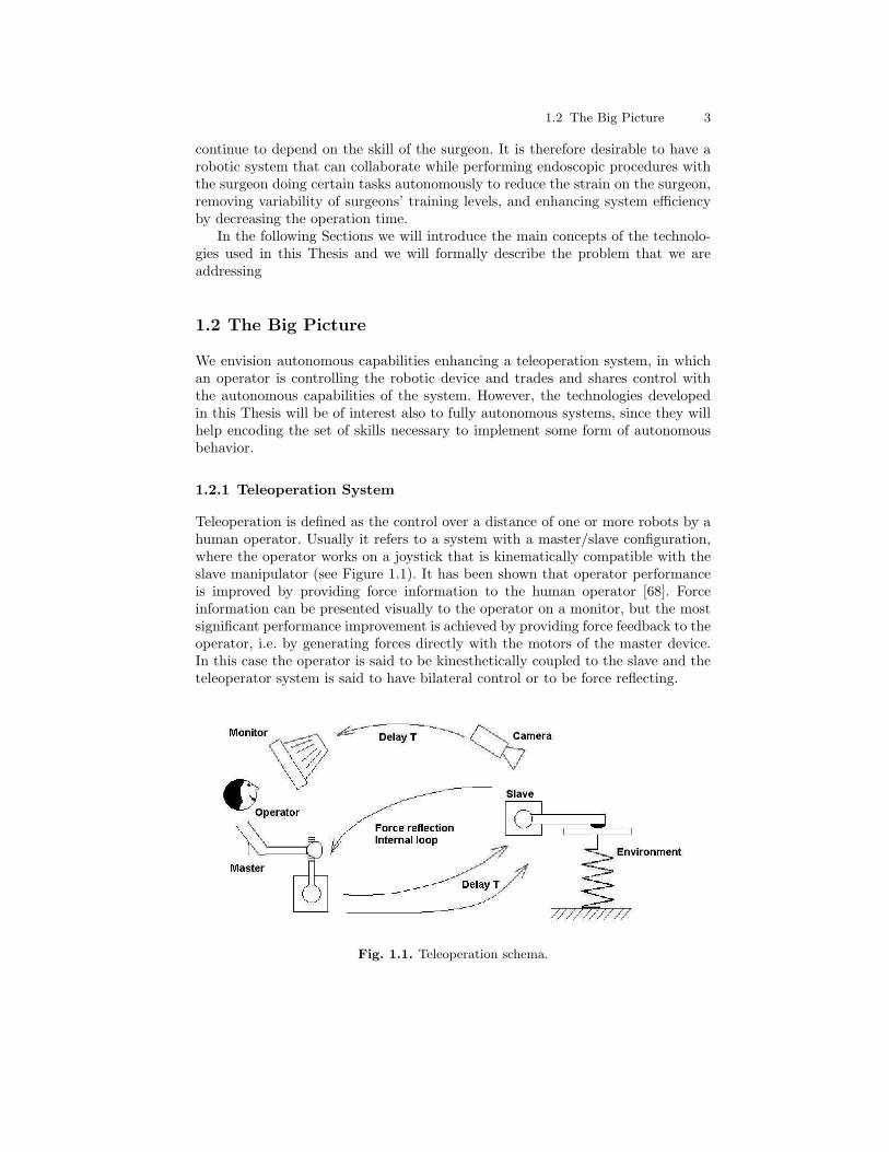
Teleoperation is defined as the control over a distance of one or more robots by ahuman operator. Usually it refers to a system with a master/slave configuration,where the operator works on a joystick that is kinematically compatible with theslave manipulator (see Figure 1.1). It has been shown that operator performanceis improved by providing force information to the human operator [68]. Forceinformation can be presented visually to the operator on a monitor, but the mostsignificant performance improvement is achieved by providing force feedback to theoperator, i.e. by generating forces directly with the motors of the master device.In this case the operator is said to be kinesthetically coupled to the slave and theteleoperator system is said to have bilateral control or to be force reflecting.
Fig. 1.1. Teleoperation schema.
4 1 Introduction
Teleoperation is used in cases where the environment is not directly accessibleby a human, or when it is too dangerous for on operator, or when it is necessaryto scale the force exerted on the environment. Almost all of the applications ofteleoperation involve contact with the remote environment, e.g. grasping, weldingand puncturing. In particular, robotic applications to surgery include puncturingas one of the most usual actions.
The trade-off between stability and performance is the main consideration inthe design of a teleoperation system. In fact, teleoperation control architecturesanalyzed in the literature can be classified in terms of their stability and perfor-mance trade-off [120]. Control algorithms for ideal kinesthetic coupling [188] areat one end of the spectrum, whereas passivity based algorithms [14] are at theother end. Conventional algorithms such as position error based force feedbackand kinesthetic force feedback lie in the middle.
Both performance and stability are inherently dependent on the task for whichthe system is designed. Thus the need to design system controllers for the specificapplications, including local and remote environments, not only in terms of param-eter tuning, but also with respect to the overall control scheme. In this Thesis wefocus on the control of a slave manipulator. In particular, we are interested in theinteraction with soft objects. The motivation for this analysis is robotic telesurgery,i.e. surgical operations performed by robotic instruments controlled by a surgeonthrough teleoperation [40, 65, 108]. One of the goals of robotic telesurgery is toimprove dexterity and perception during minimally invasive surgery through theuse of teleoperation technology [153, 174]. Clearly, the environment in which theslave manipulator moves is not completely known and organs are characterized bypartially known mechanical properties. Furthermore, by its very nature, surgeryrequires different modes of interaction during the course of an operation: for ex-ample free motion, contact and puncturing.
1.2.2 Surgical Systems
Robot-based surgical systems are starting to support surgeons during traditional aswell as experimental procedures. These systems usually consist of a control consolefrom which the surgeon issues manual or vocal commands to a robot which thenexecutes them at the nearby surgical arena. Images from the surgery are returnedto the console as the only sensory feedback available to the surgeon. In certainsystems, a separate display shows a graphical representation of the forces appliedby the robot to the patient body during the procedure. The lack of force feedbackdirectly to the surgeon’s hands is a significant drawback of today’s robotic surgicalsystems and the cause of some criticism by practicing surgeons. A similar problemis also present in simulators of laparoscopic surgery, since a computer model re-places the patient body and therefore force feedback may not be very realistic. Inthe last ten years haptic interfaces have addressed this problem, producing realisticsensations in some of current simulators. Therefore, one of today’s main challengesis the correct modeling of biological tissues. To determine the correct force feed-back to the user, the simulator must compute the tissue deformation in real time.Of course, the deformation has to be validated by biomechanical measures.
1.3 Thesis Objectives 5
An important issue of the research carried out in this work is the a priori knowl-edge, hence studies on correct force feedback and modeling of the environment werecarried out, see Chapter 8, in order to take advantages of this research.
1.3 Thesis Objectives
Due to the complex and diverse nature of a generic surgical task, the use of asingle control law for the whole task is not feasible. Therefore, we propose touse an approach based on Hybrid System theory, whereby a task is modeled asa sequence of states each endowed with its own controller. The peculiarity ofhybrid systems is the interaction between continuous-time dynamics (governed bydifferential or difference equation), and discrete dynamics and logic rules (describedby temporal logic, finite state machine, if-then-else conditions, discrete events, etc.)and discrete components (on/off switches, selectors, digital circuitry, software code,etc.) Drawbacks of this approach include the fact that the design of the controllerhave to take into account the continuous part and the discrete part (jumps).
This Thesis will address the problem of controlling such a hybrid system. Wewill consider the problem both from theoretical and practical perspectives. Ourtheoretical work will develop a mathematical model of control computation, andour practical work will develop techniques for the automation of complex task,such as surgical procedures. Since our analysis will be based on hybrid systems, wewill investigate continuous and discrete system properties. Our model for controlcomputation will be the hybrid automaton. A hybrid automaton is a state machinewith transitions between states that are governed by a discrete logic decision. Weclassify hybrid automata according to what question about their behavior can beanswered algorithmically. In particular, the class of hybrid automata that we willuse has deterministic behavior.
The properties of a control algorithm are stated in terms of satisfying stability.However, in our case stability analysis is not enough to ensure either good perfor-mance or task termination, so our purpose is also to determine a set of parametersthat can be used to determine the performance of the control system and whetheror not the task is likely to terminate. In other words we have to find what does”good” and ”bad” mean in the surgical environment and use ”bad” as a warn-ing for possible critical situations. The main difficulty of proposing a new controlmethod for an application such as robotic surgery, is to ensure complete and totalsafety of the procedure. This imply the need to address a number of aspects, which,in a less demanding application, may be overlooked in a first development. In fact,this Thesis will deal with uncertain and variable environments, as represented bythe different patient anatomies, with the true complexity of a surgical operation,without imposing unrealistic simplifications. The Thesis will also deal with thepresence and the interaction of humans to provide input to the system, and withthe difficulties of implementing the results.

6 1 Introduction
1.4 Outline and Contributions
In summary, we will develop a framework that will expand the classical theoreticalresults of dynamical system control and that will be suitable for hybrid systemscontrol. This feature should lead eventually to the extension of several controltechniques that are currently available for non-hybrid systems to hybrid systems,thus rendering the analysis of hybrid system easier and more reliable.
Because of the complexity of the problem that we want to address, we need touse a number of different theories and tools. To model the system we will adopt theframework of hybrid systems and use the hybrid automata formalism, which nicelyaccount for the mix of event and time driven dynamics characterizing task models.To develop a control for such a system, we will use the formalism of optimal control.It will allow us to use the a priori knowledge as the basis for stability analysis andfor identifying the main performance properties of the complete system. In thiswork, however, we focus on the control aspects of the complete system, studyingthe optimal control for each jump and iterating the algorithm on the completesystem.
The Thesis is organized as follows. After a brief explanation of the challengesof this project from the point of view of the autonomous execution, Chapter 2, wewill present an overview of the state of the art of the technologies that will be thebuilding blocks of this research. We will address the main aspects of the modeland an analysis of hybrid systems in Chapter 3. In Chapter 4, together with somespecific notion on suture we present the surgical aspects that are the environmentand the motivation for this work. After these concepts have been sketched, we willpropose a possible approach to the control design in Chapter 5. In Chapter 6 wediscuss numerical solution to the optimal problems with emphasis on the solutionthat we adopt in this work. Finally, in Chapter 7, we give an example of applicationand in Chapter 8 we report some teleoperation experiments with the same setupthat we are going to use for autonomous task execution experiments. In Chapter 9the summary and an indexed list of activities for the near future concludes theThesis.
2
Autonomous Task Execution
The question of whether computers can think is just like the question of whethersubmarines can swim.
Edsger W. Dijkstra
In this Chapter we will briefly summarize the state of the art of AutonomousTask Execution, i.e. the set of tools and techniques developed to guide a complextask to its completion. By complex task we mean an activity that cannot be de-scribed only in terms of reaching a set point or following a nominal trajectory, butthat requires the satisfaction of logical and algebraic conditions at the beginning,during, and at its conclusion. The conditions on the task are derived from sensormeasurements, logical states of the variables and a priori knowledge of the taskstructure. The evolution of the task must be governed by a supervisory process,which can be made explicit in the form of a monitoring agent, or implicit in thestructure and the conditions of the task itself. The quality of the task, up to itssuccessful conclusion, must be ensured and monitored by the appropriate selectionof the condition set. The Chapter reviews some of the approaches developed toaddress the various aspects of the problem of complex task modeling and control.First, a few examples are given of complex task; then we present a description ofhow the research has attempted to define and model the requirements of complextasks; finally, we review several approaches and results in the area of task model-ing, execution and monitoring. The Chapter is concluded by a few considerationson the lessons learnt in this area, which motivates the approach to complex taskcontrol described in the next Chapters.
2.1 Definitions and General Concepts
To justify the difficulties in developing an infrastructure for autonomous task exe-cution, the tasks under consideration must be extremely important and impossibleto be controlled directly by a human operator. For example, automatic task execu-tion has been implemented for the control of space probes and telerobotic devicesoperating in Earth orbit or on planet surface. Space probes in fact, are controlled
8 2 Autonomous Task Execution
by uploading a series of commands, called a sequence, which has been tested onEarth for correctness on a probe simulator [75]. Furthermore, this application doesnot support any form of interactive control and teleoperation because of the longcommunication time delay between the Earth station and the remote robot. Thisapproach has been successfully used during the Mars Pathfinder mission and pro-posed for next Mars exploration missions [21].
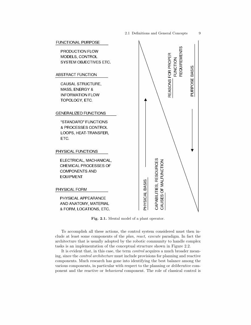
An important aspect of the tasks considered in this Thesis is that they arecomplex, i.e. cannot be controlled by Automatic Control techniques alone. Classicaland Modern Control Theory, in fact, study the design of control systems whosepurpose is to ensure that a vector of nominal trajectories is closely tracked by thecontrolled plant. The trajectories are continuous functions of time and the controlactions aims at reaching an equilibrium in which the error vector goes to zero.Instead, a complex task has a structure that can be represented by the diagramin Figure 2.1. This Figure shows the mental model developed by the operators ofcomplex systems, such as nuclear and power plants, to help manage the complexityof the operations and the flow of data [124,150,151]. The task, in this case, is thecorrect operation of the complete plant.
In these studies, the authors set the basis for the definition of the mental modelof a complex task, and formulate a hypothesis on how a person interacting with thetask organize the task mental representation. The hypothesis proposed is that thethe task model has a layered structure, in which each level has a different degreeof data abstraction. Each level processes a specific type of feedback, from rawmeasurements to plant states, so that the amount of data remains approximatelyconstant at every level. With this representation, the operator can process plantinformation at each level, and in particular can initiate a control action at the levelin the hierarchy whose data representation best describes the current situation andsupports the required corrective action. In this way, for instance, an alarm signalcan trigger a response action at the lowest level, without interacting with the higherlevels because its importance is recognized immediately. A drift in the state of theplant instead, needs to be processed at a higher level in the hierarchy, becauseit is characterized by the combination of several feedback signals possibly filteredby logical operators. With such a structure, the operator adds three importantfeatures to the plant’s mental model that improve her/his control performance:causal connections between layers, constant data complexity, and directed focusof attention.
Figure 2.1 as also been used as a model of the robot control paradigm plan, re-act, execute that is currently at the heart of most robotic systems. In this paradigm,the Automatic Control functions are confined to the bottom layer of the architec-ture, whereas techniques of Artificial Intelligence are more appropriate for theupper layers. The tasks considered in this Thesis, although much simpler than thecontrol of a power plant, require the careful integration of execution and sens-ing functions, but also of reactions to unexpected events and planning completesequences of actions. Data will be a mixture of continuous and logical signals gen-erated by sensors and by higher level cognitive functions. Typically, these tasks willinclude some motion phase, some interaction with the environment, some sensorbased input, and some adaptation to an uncertain environment.
2.1 Definitions and General Concepts 9
Fig. 2.1. Mental model of a plant operator.
To accomplish all these actions, the control system considered must then in-clude at least some components of the plan, react, execute paradigm. In fact thearchitecture that is usually adopted by the robotic community to handle complextasks is an implementation of the conceptual structure shown in Figure 2.2.
It is evident that, in this case, the term control acquires a much broader mean-ing, since the control architecture must include provisions for planning and reactivecomponents. Much research has gone into identifying the best balance among thevarious components, in particular with respect to the planning or deliberative com-ponent and the reactive or behavioral component. The role of classical control is
10 2 Autonomous Task Execution
Perception Signals
Storedrules
Identification Decision Planning
Recognition
Actuation
Symbols
Signs
Skill level
Rule level
Knowledgelevel
State
task
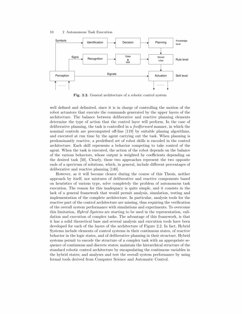
Fig. 2.2. General architecture of a robotic control system
well defined and delimited, since it is in charge of controlling the motion of therobot actuators that execute the commands generated by the upper layers of thearchitecture. The balance between deliberative and reactive planning elementsdetermine the type of action that the control layer will perform. In the case ofdeliberative planning, the task is controlled in a feedforward manner, in which thenominal controls are precomputed off-line [119] by suitable planing algorithms,and executed at run time by the agent carrying out the task. When planning ispredominantly reactive, a predefined set of robot skills is encoded in the controlarchitecture. Each skill represents a behavior competing to take control of theagent. When the task is executed, the action of the robot depends on the balanceof the various behaviors, whose output is weighted by coefficients depending onthe desired task [50]. Clearly, these two approaches represent the two oppositeends of a spectrum of solutions, which, in general, include different percentages ofdeliberative and reactive planning [140].
However, as it will become clearer during the course of this Thesis, neitherapproach by itself, nor mixtures of deliberative and reactive components basedon heuristics of various type, solve completely the problem of autonomous taskexecution. The reason for this inadequacy is quite simple, and it consists in thelack of a general framework that would permit analysis, simulation, testing andimplementation of the complete architecture. In particular, analysis tools for thereactive part of the control architecture are missing, thus requiring the verificationof the overall system performance with simulations and experiments. To overcomethis limitation, Hybrid Systems are starting to be used in the representation, vali-dation and execution of complex tasks. The advantage of this framework, is thatit has a solid theoretical base and several analysis and execution tools have beendeveloped for each of the layers of the architecture of Figure 2.2. In fact, HybridSystems include elements of control systems in their continuous states, of reactivebehavior in the logic states, and of deliberative planning in their structure. Hybridsystems permit to encode the structure of a complex task with an appropriate se-quence of continuous and discrete states; maintain the hierarchical structure of thestandard robotic control architecture by encapsulating the continuous variables inthe hybrid states; and analyses and test the overall system performance by usingformal tools derived from Computer Science and Automatic Control.
2.2 Early Work in Autonomous Task Planning and Execution 11
To show how the research in this area has evolved in the past years, in thenext Sections we will first summarize earlier work in task planning and execution,where deliberative, reactive and executive control were kept separate and graduallymixed together. Then we will describe in some detail more recent work in taskplanning and execution, where the awareness of the capabilities of Hybrid Systemsfor autonomous task execution is becoming more evident.
2.2 Early Work in Autonomous Task Planning andExecution
Earlier formalizations and architectures developed to describe and execute complextasks included a variety of tools and procedures, but little emphasis is given tostructured approaches.
Some of the earlier solutions proposed address the need of intelligent dataacquisition and processing, i.e. the development of sensors capable of producingalso a logical output from the data collected. This approach was called the Logi-cal Sensor Specification [103], in which physical devices were separated from eachother and from the central controller by software layers, where local processing offeedback signals and actuator commands could take place. Other proposals putmore emphasis on the local reactive capabilities of the controlled system and theyused mechanical devices able to produce an implicit control similar to the HumanReflex Action [30]. These approaches were directed to solve specific problems, andtherefore more general structures were studied based on Expert Systems [173,121]or on Artificial Neural Networks [54,86]. The first family of solutions permits thesystem to learn some of its own control procedures and the modularity of the rulebase allows for easy implementation and update. The second approach is directedtowards integrating real time performance with some strategic knowledge. Finallyan important area of research was Intelligent Control [51, 136], in which nestedcontrol loops organized in the hierarchical structure described in Figure 2.2 super-vise all aspects of the task evolution. Intelliget control is still a general approach,proposed for a number of different applications and is not specific to robotics.However, because of this fact, it is still very application dependent and cannoteasily extended to generic robotic tasks.
To address the need of higher flexibility, with specific reference to the controland execution of robotic tasks, a new approach was proposed in the context ofthe Telerobotic Testbed, described in [100], which was a telerobotics laboratorydeveloped at JPL-Caltech under NASA sponsorship, completely devoted to thedevelopment of new control strategies for telerobotic tasks. During the develop-ment of the testbed, teleoperation capabilities were enhanced with the addition ofdextrous manipulators [23], dual-arm operation [99], and automatic sequence gen-eration and execution. This last development is relevant to the research describedin this Thesis since it represents an approach to formulate and execute a sequenceof operations in a partially structured environment. Tasks were built interactivelyusing a series of pre-programmed skills such as, guarded motion, move-to-push,slide, insert, and so on [22], i.e. all actions that could be framed in the context ofclassical control algorithms. Skills were parameterized, so that different operations
12 2 Autonomous Task Execution
could be programmed using the same set of basic capabilities. The execution ofthe sequence was carried out by maintaining two queues of commands, one re-quiring only feedforward commands and the other requiring some feedback fromthe sensors, called Reflex Actions [24]. The execution of each skill was monitoredby defining termination conditions on each controlled variable. The description ofthe complete system, with sequence input and execution, and a discussion of ro-bustness issues during execution is presented in [25]. This approach was tested inlaboratory experiments of complex sequences: opening Orbital Replacement Unit(ORU) door, and turning bolts were successfully completed. However it is not clearhow much engineering of the environment went into ensuring that the task, i.e. thecomplete sequence of skills, completed successfully. Furthermore, the uncertaintyrelative to the task is compensated by defining ranges, rather than values, of theparameters, but without including additional states into the task model.
All the approaches presented in this Section share the common aspect of beingdeveloped for a specific task, without a unifying framework for task analysis andcontrol and thus are examples of ad hoc solutions rather than instances of a formaltheory of complex system analysis and control. In the next Section we will brieflyreview some of the more recent results in task control and show how the field isevolving towards a more extensive use of the formalism of Hybrid Systems.
2.3 Recent Work in Autonomous Task Planning andExecution
As mentioned in the previous Section, the main limitation emerged from the sum-mary of the earlier work, is the lack of a structured approach to the analysis andcontrol of a complex task. In this Section we trace the more recent development,leading to the gradual establishment of the Hybrid System methodology as thecomprehensive framework for complex task study. In particular, one of key the-oretical element missing in the earlier work is the tight and effective integrationof deliberative and reactive planning with execution and control. In this Sectionwe will briefly summarize a few approaches showing how this problem is beingaddressed, and will describe solutions that respond to this need with various levelsof integration. The approaches presented in this Sections are subdivided accordingto the technology that they address: single sensing and control actions, or globalarchitectural issues.
2.3.1 Design, Sensing and Actuation Issues
Clearly, the main issues of complex task control are related to the architectureand communication characteristics of the control system. However, also the basicelements of the architecture, such as sensors and actuators, must be capable ofresponding to the demands of the architecture. In this Section, we briefly documentsome of the enhancements made to robotic devices to make them compatible withthe needs of complex task control. In particular, we first describe an example ofadvanced processing at the low level of the architecture, then at the middle level,and finally in the top layer of the architecture.
2.3 Recent Work in Autonomous Task Planning and Execution 13
The issues of integrating actuation and perception at the low level of the con-trol architecture is addressed by the approaches summarized next. Visual servoingis a form of trajectory control in which feedback data are produced by imageprocessing, thus providing a form of feedback control higher than standard signalprocessing. The approach described in [115], presents a few experiments in thisarea, with reference to the surgical robotics domain, in which the motion of a la-paroscopic instrument is guided using the image of a laparoscopic camera. In theseexperiments, the higher level of the reference architecture of Figure 2.2 is suppliedby the human operator, who teleoperates the surgical instruments with the helpof visual servoing. Thus, this technique can be described as a semi-autonomousenhancement to teleoperation. To achieve the motion of the instruments, the au-thors designed a new instrument-holder equipped with laser beams projecting aknown pattern on the internal surfaces of the patient. This pattern, once properlyidentified and measured, is the basis of visual servoing, since it identifies the cur-rent position of the instrument in the patient’s body and allows to safely movethe instrument even when it is not in the field of view of the endoscopic camera.With this set up, the surgeon can specify the final position of the instrument tipby indicating it on the monitor with a cursor, and bring it to a desired positionwithout an exact knowledge of its current position. The technology described inthe paper is an example of essential technologies for autonomous task execution,since it provides the low level sensing and actuation necessary to give the bottomlayer of the architecture the desired processing autonomy.
The needs of the middle layer of the architecture shown in Figure 2.2, namelythe capability of adapting a planned task execution to variations of the task pa-rameters are addressed in [39]. Here, the authors describe an example of reactivecontrol methods applied to a robotic surgical task. Reactive control is impementedby means of a new device, the EndoBot, which can provide some form of sharedand traded control during a MIS procedure. The EndoBot consists of a dockingstation holding two four-degree-of-freedom devices, each capable of moving a MISinstrument along four axes, since two axis are constrained by the incision point.The device was designed to cooperate with the surgeon, in the sense that the sur-geon could teleoperate some of the axes and the robot can move the other axesautonomously. The approach relevant to this Thesis is the role of the device dur-ing a simple suture in which it compensates autonomously unexpected variationsin the environment. However no explanation is given on how the EndoBot wouldautonomously execute the suture and what sensory conditions and motor controlswere used to progress from one phase to the next.
At the upper level of the reference architecture, there is a planning layer that isin charge computing the initial nominal task trajectory. One of the main problemarising with this configuration is the division of activities between the middlelevel, i.e. the reactive planner/behavior, and the top level. In particular it must bedecided at what point the nominal task trajectory need to be completely replannedand the local corrections applied by the middle level are no longer sufficient toensure task conclusion. An example of the solution to this problem is presentedin [20] in the context of the autonomous landing of an airship. The task here iscarried out using pure visual servoing, and is a complex control problem requiringa system with a good level of autonomy. In this case the autonomy is necessary to
14 2 Autonomous Task Execution
compensate the severe disturbances of wind gusts, which require the replanning ofthe landing maneuvers when the trajectory exceeds a given tolerance.
Another type of autonomy is discussed in reference [80] where an approach ispresented in which the telerobotic system improves the way the operator’s com-mands are executed by the remote robot, by varying the ratio between the com-manded and the executed velocities of the robot. In this way, for example, the robotcan autonomously adjust the approach velocity of the robot to a target to improveaccuracy and overall performance. This approach is demonstrated in several Fitts’law1 [88] type experiments. When replannig is too difficult for an automatic agent,a human operator can be called upon for help, and the control functions can beshared between the robot controller and a human operator, as described in [84].In this case, the operation of the robot is mostly autonomous, and the task is theassembly of micro MEMS components. However there are situations in which therobot cannot operate autonomously, for example when the uncertainties in themicroassembly are different from those considered when developing an assemblyplan. The robot then requires human assistance and, depending on the case, thecontrol can be shared between the robot and the operator, or traded, with fullcontrol given to the human. In this research
Another aspect of complex task analysis refer to the preliminary modeling ofthe task structure. A correct model is essential to express the a priori knowledgeabout the task and to set up the various task evolution scenarios. An approach torepresent manipulation tasks in a formal manner is described in [29]. The paperdescribes a set of grasping tasks in terms of the way humans carry them out. Thepreferences of several human subjects are coded into a knowledge base, which isthen used to different grasp patterns in terms of grasping primitives. The primitivesare also classified according to the shape of the object to be grasped and the typeof robot hand. The task is represented as a set of discrete rules, that shouldbe used by a controller as pre and post conditions to the various phases of agrasping task. In this example, the grasp patterns are the different instances of agrasp task, whereas the grasp primitives represent the behavior level of the taskcontrol. Another example of task modeling is described in [27] in the context ofmanufacturing operations. In this research, an assembly task is described by meansof a graph in which nodes and edges represent the various objects involved and theactions required. However, this method does not enter into the detail of how thesequence of actions described should be executed and controlled by an automaticdevice. In any case, the definition of a task as an oriented graph is one of thecurrent methods used to specify the task structure and execution flow.
Having briefly discussed the single elements and technologies concurring tothe implementation of the control of a complex task, in the next Section we willexamine the structure of the software system that must be set up to supportadvanced control functions.
1 Fitts’ law is a model of human psychomotor behavior developed in 1954. Accordingto Fitts’ Law, the time to move and point to a target of width W at a distance A is alogarithmic function of the spatial relative error (A/W ).
2.3 Recent Work in Autonomous Task Planning and Execution 15
2.3.2 Architectural Issues
Key to the effective operation of a task-level control system is the underlyingsoftware architecture and the mechanisms governing the exchange of functionsand duties among the different agents in the control system. This is a very activeresearch area which is currently being explored by a number of large projects,both in Europe and in the US, and a small sample of the results achieved so far isdiscussed next.
An effective balance of feedforward and feedback control is described in [157]where the authors presents the analysis and implementation of the control systemfor two different tasks, walking and object grasping. In this paper the authorsdescribes the network of actions and the logical checks that form the Task ControlArchitecture used for the two tasks. It is interesting to note that the control isbased upon a rather fix task model, in which a set of concurrent control actionsare executed at different frequencies to ensure some concurrency. Although ratherpowerful, this approach seems to encode the tasks in the control and may requiresubstantial modification to be used to control a different task. Thus the deliberativecomponent of planning is represented by the task tree and the a priori knowledgeby the sequence of task actions. The issue of modifying the task to adapt to achanged environment seems not to be addressed in detail.
A different approach is described in [26] in which the authors describe anarchitecture for the motion control of a group of autonomous vehicles based onthe careful tuning of various behaviors. In this paper, the task demanded to therobots is the exploration of an area, and therefore it involves almost exclusivelythe motion of robots while keeping an assigned formation. In this case, the taskis coded in terms of the robot formation and the maneuver goal. Because of thelinearity of the task it is acceptable to have a preponderance of reactive behaviorversus deliberative planning. It is questionable whether this approach is applicableto more structured tasks, where temporal and spatial sequences of actions mustbe combined to complete the task.
Another exmple of an architecture based on the behavior paradigm for plan-ning and control is described in [9] in the context of exploring and mapping anindoor environment. The behaviors implemented for the task of map formation,are go to, obstacle avoidance, wall avoidance, corridor following, door passing, anddocking to reach the recharging station. However, in this case the mapping taskis specified in two forms. The actual measurements and memorization of the envi-ronment is carried out autonomously by the robot, whereas the higher functions ofnavigation and exploration patterns are not performed autonomously, but replacedby following a human guiding the robot through the environment, thus allocatingresources according to the ability of an agent to perform the function.
An implementation of the deliberative and reactive framework in autonomoustask execution is described in [19], where the authors describe in detail the imple-mentation of a robot control architecture consisting of three main layers: planning,execution, and reaction. The first layer takes care of the definition of the high levelgoals using the environmental map. The execution layer partitions the goals intosubgoals and activates the appropriate behaviors. Finally, the reactive layer inter-faces the robot with sensors and actuators and modifies the plans in real time. Thearchitecture proved very successful in an exhibition where the robots traveled more
16 2 Autonomous Task Execution
than 3000 Km. However, tasks executed by the robots had not a fixed configura-tion and can be rearranged depending on the various sensor input. Furthermore,no manipulation was involved, thus constraints on task execution were somehowsimpler to model and satisfy, and the switch to the deliberative planner was onlyrequired to compute a new navigation trajectory in the environment.
The integration of vision and grasp planning and execution is described in [114].The authors describe the experiments carried out to verify the performance of avision-based tracking system combined with a grasp planner. The tracking systemis used to estimate pose and motion direction of an object, and provides these datato the grasp planner, which then plans a stable grasps and commands a robotichand to execute. The integration of vision and grasping is a key element in thedevelopment of autonomous manipulation tasks and this paper describes the adhoc architecture used to carry out the task.
Failure recovery and graceful degradation are important issues in the contextof complex tasks, where safety may be crucial. Since, in most cases, complex tasksare carried by independent agents, safety depends on the correct functioning ofall the agents. However, since malfunctions do occur, it is important to identifyin which way a group of agents can gracefully alter its operation to maintainits basic capabilities. These same considerations can be extended also to roboticteams, as discussed in [76], where the authors examine the main causes of mal-functions: communication failure, robot partial malfunction, and robot death. Theapproach discussed is based on capitalistic market economy, a flavor of game the-ory, in which each robot is an independent agent trying to maximize its own good.However, since the payoff depends only on the team success, the satisfaction ofthe team goal equates to maximization of each individual profit. Using this ap-proach, the authors show the capability of the team to reconfigure its resourcesas a function of detected failures and the team ability to carry out autonomouslythe assigned task, even in the presence of several failures. In this example, bothdeliberative and reactive planning are carried out in an implicit form, resultingfrom the optimization algorithms implemented in the control software.
The main criticism one can move to the approaches presented above, and tomainstream research in this area is the lack of a unifying method to study complextasks, whether during modeling, analysis and, finally, execution. A possible answerto this lack of common theoretical background is given by the increasing use ofHybrid System methodologies to support the description and the execution ofautonomous tasks.
A typical example of how this formalism can be used in the context of complextask control is given in [143]. The application described in the paper refers tothe everyday action of opening a door, but it integrates different control andsensory modalities of the type needed in the real autonomous surgical procedure,which are the main focus of this Thesis. The paper first gives a model of the opendoor task, in which each action of the task is assigned to a specific control modeand qualified by appropriate sensor thresholds to ensure completion. The task isdescribed using the Hybrid System formalism and the control parameters neededin each continuous state of the Hybrid Model are estimated on line during taskexecution. The authors indicate that experiments carried out with this approachwere successful about 90% of the time, mostly due to the lack of an accurate error
2.3 Recent Work in Autonomous Task Planning and Execution 17
recovering strategy. The challenge in this case is to extend this approach to morecomplex cases, such as medical procedures, where safety is paramount.
Other examples of use of the Hybrid System formalism in complex task analy-sis and control is represented by the following papers. In [57] the authors describethe implementation of a robot capable of autonomous installing warning sphereon high voltage cables. In this case, the task to be carried out by the robot is welldefined and the authors do not provide much detail on how the various phasesof the task are controlled by the underlying hybrid system monitor. In [62, 63] ahybrid automaton is used to model the cooperation of multiple mobile robots toperform a coordinated manipulation. In [62] each robot of a team is assigned arole and the dynamic exchange of the roles during the execution of the cooperativemanipulation of an object is governed by a hybrid automaton. A suitable utilityfunction determines when and to what role a robot should be assigned, and sim-ulations show that this policy supports the execution of the task. The novelty ofthe approach presented in [63] is in the composition of the hybrid automata rep-resenting each individual robot into a single, more complex, automaton describingthe complete cooperative task. The authors point out the possibility of doing for-mal task analysis and verification using the hybrid system methodology to identifypossible faults and deadlocks in the task execution.
Finally, another area of application of Hybrid System theory, and of greatpotential impact, is the control of the navigation and interaction of autonomousvehicles. An example is [7], in which the authors summarize their contributionsto this research area. The focus here is on intelligent multi agent systems thateventually will replace centralized control systems, as in the case of air trafficmanagement, or will enhance human resources, as in the case of automatic vehiclecontrol. The Hybrid System framework is ideally suited for autonomous, or semi-autonomous, agent control. In fact, at the continuous level, each agent choosesits own optimal strategy, while discrete coordination is used to solve conflicts.This approach has several advantages with respect to centralized control: has thepotential to yield an optimal design, it is intrinsically reliable and scalable, andis flexible to adapt to different conditions, traffic levels, and unexpected needs. Inthe context of traffic management, the Hybrid System definition of safe sets, has avery real meaning, since it represents the state set able to guarantee, for example,collision avoidance. In particular, a hybrid automaton can be used to representthe different operating conditions of the autonomous vehicle, and thus frame andrepresent in a consistent way the discontinuities of navigation control.
Concluding this brief summary of approaches and techniques to the architec-tural design of complex task control systems, it appears that the methods satisfy-ing most of the requirements on model definition, formal analysis, simulation andexecution are based on some variation of the Hybrid System methodology. Thismethodology, as it is discussed in the next Chapters, is still in its infancy andtherefore it has not yet reached a unified and all encompassing structure. It is stilla collection of many similar definitions and methods, yet the techniques developedso far are very relevant and useful to the objective of this Thesis.
18 2 Autonomous Task Execution
2.4 Conclusions
In this Chapter the main issues and developments relevant to autonomous taskexecution have been briefly described. First the distinction between simple andcomplex tasks has been addressed, and then some of the difficulties found in thedevelopment of autonomous systems listed in terms of modeling, analyzing, andexecuting the sequence of actions representing a complex task. To show how thisproblem has been addressed by many researchers in the past twenty years, firstearlier work is summarized to show the variety of solutions proposed. Then, mostrecent papers are summarized emphasizing the clear trend emerging towards thedevelopment of a mathematical framework able to support all the needs in complextask planning and control. The current trend is towards the adaptation of HybridSystem methodologies to the needs of complex task execution and control. Thistrend is illustrated by pointing out the results described in a few key papers in thearea. In the following Chapters, this trend will be further justified, by analyzingthe advantages offered by the Hybrid System methodology in the development ofa control strategy for a surgical suture.
3
Hybrid System
Everything should be made as simple as possible, but not simpler.Albert Einstein
The hybrid systems of interest in this research are dynamic systems, where thebehavior of interest is determined by the interaction of continuous and discretedynamics.
There are several reasons for using hybrid models to represent the dynamicbehavior of a complex task. Reducing complexity is an important reason for dealingwith hybrid systems; this is accomplished by incorporating models of dynamicprocesses having different levels of abstraction. For example a thermostat typicallysees a very simple model of the complex heat flow dynamics adequate for thetask in hand. Another example is the analysis of non linear systems. In orderto avoid dealing directly with the set of nonlinear equations, one may choose towork with sets of simpler equation (e.g., linear), and switch among these simplermodels. The advent of digital machines has made hybrid systems very commonindeed. Whenever a digital device interacts with the continuous world, the behaviorinvolves hybrid phenomena that need to be analyzed and understood.
It is not hard to find examples of systems that motivate the need for studyinghybrid systems. Many examples can be found in the literature, for instance themanagement of a fishery resource [141], computer disk system [92], motion controlsystems [49], robotics (a non exhaustive list [78,83,163,184]), power systems [105],systems in classical mechanics [48], air traffic management [172] and automatedvehicles [127].
In this chapter we will give a brief overview of the main aspects of the modeland analysis of Hybrid Systems, that will form the framework for this research.
3.1 Survey of systems and model
Construction of models (abstractions) of parts of reality (systems) and investiga-tion of their properties are fundamental issues for all scientists. The models canbe more or less formal but all have the property that they try to link relations
20 3 Hybrid System
in the system to some kind of pattern. Loosely speaking, a model of a system isa tool used to represent some sort of knowledge of the system without makingexperiments. It is used for instance to predict the future behavior or to design acontroller. The degree of agreement between the system and the model determinesthe usefulness of the model. One of the tasks of applied mathematics is to gener-ate models for the description of systems in different disciplines. A mathematicalmodel formally describes the relation between different quantities and variables inthe system by a mathematical relation. Such models are commonly used in modernengineering science, for instance control engineering and computer science, and arethe class of models studied in this Thesis.
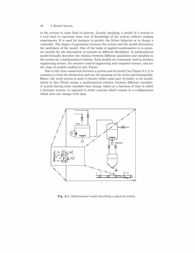
Due to the close connection between a system and its model (see Figure 3.1) it iscommon to drop the distinction and use the meaning of the terms interchangeably.Hence, the word system is used to denote either some part of reality or its model,which in this Thesis means a mathematical relation between different variables.A system having state variables that change values as a function of time is calleda dynamic system, as opposed to static systems which remain in a configurationwhich does not change with time.
Fig. 3.1. Mathematical model describing a physical system.
3.1 Survey of systems and model 21
3.1.1 Classification of Dynamic Systems
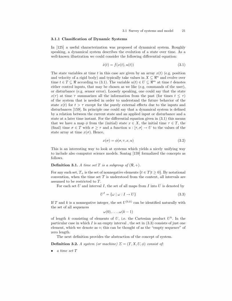
In [125] a useful characterization was proposed of dynamical system. Roughlyspeaking, a dynamical system describes the evolution of a state over time. As awell-known illustration we could consider the following differential equation:
x(t) = f(x(t), u(t)) (3.1)
The state variables at time t in this case are given by an array x(t) (e.g. positionand velocity of a rigid body) and typically take values in X ⊆ <n and evolve overtime t ∈ T ⊆ < according to (3.1). The variable u(t) ∈ U ⊆ <m at time t denoteseither control inputs, that may be chosen as we like (e.g. commands of the user),or disturbance (e.g. sensor error). Loosely speaking, one could say that the statex(τ) at time τ summarizes all the information from the past (for times t ≤ τ)of the system that is needed in order to understand the future behavior of thestate x(t) for t > τ except for the purely external effects due to the inputs anddisturbances [159]. In principle one could say that a dynamical system is definedby a relation between the current state and an applied input or disturbance and astate at a later time instant. For the differential equation given in (3.1) this meansthat we have a map φ from the (initial) state x ∈ X, the initial time τ ∈ T , the(final) time σ ∈ T with σ ≥ τ and a function u : [τ, σ] → U to the values of thestate array at time x(σ). Hence,
x(σ) = φ(σ, τ, x, u) (3.2)
This is an interesting way to look at systems which yields a nicely unifying wayto include also computer science models. Sontag [159] formalized the concepts asfollows.
Definition 3.1. A time set T is a subgroup of (<,+).
For any such set, T+ is the set of nonnegative elements t ∈ T |t ≥ 0. By notationalconvention, when the time set T is understood from the context, all intervals areassumed to be restricted to T .
For each set U and interval I, the set of all maps from I into U is denoted by
U I = ω | ω : I → U (3.3)
If T and k is a nonnegative integer, the set U [0,k) can be identified naturally withthe set of all sequences
ω(0), . . . , ω(k − 1)
of length k consisting of elements of U , i.e. the Cartesian product Uk. In theparticular case in which I is an empty interval , the set in (3.3) consists of just oneelement, which we denote as ; this can be thought of as the “empty sequence” ofzero length.
The next definition provides the abstraction of the concept of system.
Definition 3.2. A system (or machine) Σ = (T,X,U, φ) consist of:
• a time set T
22 3 Hybrid System
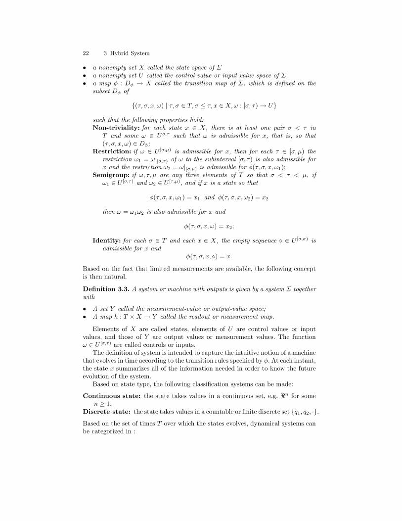
• a nonempty set X called the state space of Σ• a nonempty set U called the control-value or input-value space of Σ• a map φ : Dφ → X called the transition map of Σ, which is defined on the
subset Dφ of
(τ, σ, x, ω) | τ, σ ∈ T, σ ≤ τ, x ∈ X,ω : [σ, τ) → U
such that the following properties hold:Non-triviality: for each state x ∈ X, there is at least one pair σ < τ in
T and some ω ∈ Uσ,τ such that ω is admissible for x, that is, so that(τ, σ, x, ω) ∈ Dφ;
Restriction: if ω ∈ U [σ,µ) is admissible for x, then for each τ ∈ [σ, µ) therestriction ω1 = ω|[σ,τ) of ω to the subinterval [σ, τ) is also admissible forx and the restriction ω2 = ω|[σ,µ) is admissible for φ(τ, σ, x, ω1);
Semigroup: if ω, τ, µ are any three elements of T so that σ < τ < µ, ifω1 ∈ U [σ,τ) and ω2 ∈ U [τ,µ), and if x is a state so that
φ(τ, σ, x, ω1) = x1 and φ(τ, σ, x, ω2) = x2
then ω = ω1ω2 is also admissible for x and
φ(τ, σ, x, ω) = x2;
Identity: for each σ ∈ T and each x ∈ X, the empty sequence ∈ U [σ,σ) isadmissible for x and
φ(τ, σ, x, ) = x.
Based on the fact that limited measurements are available, the following conceptis then natural.
Definition 3.3. A system or machine with outputs is given by a system Σ togetherwith
• A set Y called the measurement-value or output-value space;• A map h : T ×X → Y called the readout or measurement map.
Elements of X are called states, elements of U are control values or inputvalues, and those of Y are output values or measurement values. The functionω ∈ U [σ,τ) are called controls or inputs.
The definition of system is intended to capture the intuitive notion of a machinethat evolves in time according to the transition rules specified by φ. At each instant,the state x summarizes all of the information needed in order to know the futureevolution of the system.
Based on state type, the following classification systems can be made:
Continuous state: the state takes values in a continuous set, e.g. <n for somen ≥ 1.
Discrete state: the state takes values in a countable or finite discrete set q1, q2, ·.
Based on the set of times T over which the states evolves, dynamical systems canbe categorized in :
3.1 Survey of systems and model 23
Continuous time: T is a continuous set, e.g. a subset of <.Discrete time: T is a discrete set, e.g. a subset of the integers Z.
Third, we distinguish systems, based on the mechanism that drives their evolution,which can be:
Time-driven: the state of the system changes as time progresses, i.e. continu-ously (for continuous time systems), or at every tick of the clock (for discretetime systems). It is common to have a model described by a continuous timecontinuous state system expressed by a differential equation (3.1). These sys-tems are usually referred to as continuous systems.
Event-driven: the state of the system changes due to the occurrence of anevent. An event corresponds to the start or the end of an activity. In gen-eral, event-driven systems are asynchronous and the event occurrence timesare not equidistant. Typical examples of event-driven systems are manufac-turing systems, telecommunication networks, parallel processing systems, andlogistic systems. For a manufacturing system possible events are: the com-pletion of a part on a machine, a machine breakdown, or a buffer becomingempty.
We can also have combinations of continuous and discrete states, of continuousand discrete time, or of time-driven and event-driven dynamics. The resultingsystems are called hybrid. In this Thesis a hybrid system essentially is a systemthe evolution of which is over continuous time, but there are also discrete timeinstants when “something happens” (e.g., the occurrence of an event that resultsin a mode change of the system. Usually the mode is then characterized by adiscrete state variable).
3.1.2 Discrete Event Systems
Discrete Event Systems (DES) are models that arise naturally for a large class ofsystems, mostly man-made and highly complex. The interest in discrete event sys-tems in control engineering has been intensified in the last decade, and a referencedescribing their properties is for example [5].
The DES mathematical models is described by asynchronous discrete-time dis-crete state systems, where the times tk ∈ < | k ∈ N are not known a priori.
Automata or finite state machines are the most common models for discretetime and discrete state (event-driven) systems, see Figure 3.2. We need some no-tation before we can give a formal definition of automaton. For a set V we denotethe collection of all subsets of V (the power set) by P (V ). Moreover, if we have twosets V and W a partial function from V to W is a mapping that is not necessarilydefined for all values of V , but only for a subset D of V (its domain). Hence, if fis a partial function from V to W , then there is a subset D(f) ⊆ V such that f isa function from D(f) to W .
Definition 3.4. An Automaton is defined by the triple Σ = (Q,U, φ) with
• Q a finite or countable set of discrete states;• U a finite or countable set of discrete inputs or the input alphabet;
24 3 Hybrid System
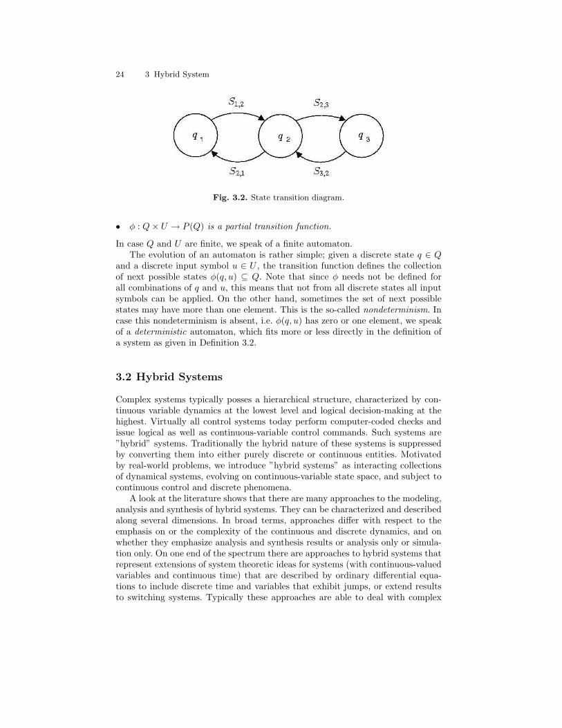
Fig. 3.2. State transition diagram.
• φ : Q× U → P (Q) is a partial transition function.
In case Q and U are finite, we speak of a finite automaton.The evolution of an automaton is rather simple; given a discrete state q ∈ Q
and a discrete input symbol u ∈ U , the transition function defines the collectionof next possible states φ(q, u) ⊆ Q. Note that since φ needs not be defined forall combinations of q and u, this means that not from all discrete states all inputsymbols can be applied. On the other hand, sometimes the set of next possiblestates may have more than one element. This is the so-called nondeterminism. Incase this nondeterminism is absent, i.e. φ(q, u) has zero or one element, we speakof a deterministic automaton, which fits more or less directly in the definition ofa system as given in Definition 3.2.
3.2 Hybrid Systems
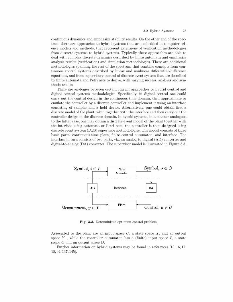
Complex systems typically posses a hierarchical structure, characterized by con-tinuous variable dynamics at the lowest level and logical decision-making at thehighest. Virtually all control systems today perform computer-coded checks andissue logical as well as continuous-variable control commands. Such systems are”hybrid” systems. Traditionally the hybrid nature of these systems is suppressedby converting them into either purely discrete or continuous entities. Motivatedby real-world problems, we introduce ”hybrid systems” as interacting collectionsof dynamical systems, evolving on continuous-variable state space, and subject tocontinuous control and discrete phenomena.
A look at the literature shows that there are many approaches to the modeling,analysis and synthesis of hybrid systems. They can be characterized and describedalong several dimensions. In broad terms, approaches differ with respect to theemphasis on or the complexity of the continuous and discrete dynamics, and onwhether they emphasize analysis and synthesis results or analysis only or simula-tion only. On one end of the spectrum there are approaches to hybrid systems thatrepresent extensions of system theoretic ideas for systems (with continuous-valuedvariables and continuous time) that are described by ordinary differential equa-tions to include discrete time and variables that exhibit jumps, or extend resultsto switching systems. Typically these approaches are able to deal with complex
3.2 Hybrid Systems 25
continuous dynamics and emphasize stability results. On the other end of the spec-trum there are approaches to hybrid systems that are embedded in computer sci-ence models and methods, that represent extensions of verification methodologiesfrom discrete systems to hybrid systems. Typically these approaches are able todeal with complex discrete dynamics described by finite automata and emphasizeanalysis results (verification) and simulation methodologies. There are additionalmethodologies spanning the rest of the spectrum that combine concepts from con-tinuous control systems described by linear and nonlinear differential/differenceequations, and from supervisory control of discrete event system that are describedby finite automata and Petri nets to derive, with varying success, analysis and syn-thesis results.
There are analogies between certain current approaches to hybrid control anddigital control systems methodologies. Specifically, in digital control one couldcarry out the control design in the continuous time domain, then approximate oremulate the controller by a discrete controller and implement it using an interfaceconsisting of sampler and a hold device. Alternatively, one could obtain first adiscrete model of the plant taken together with the interface and then carry out thecontroller design in the discrete domain. In hybrid systems, in a manner analogousto the latter case, one may obtain a discrete event model of the plant together withthe interface using automata or Petri nets; the controller is then designed usingdiscrete event system (DES) supervisor methodologies. The model consists of threebasic parts: continuous-time plant, finite control automaton, and interface. Theinterface in turn consists of two parts, viz. an analog-to-digital (AD) converter anddigital-to-analog (DA) converter. The supervisor model is illustrated in Figure 3.3.
Fig. 3.3. Deterministic optimum control problem.
Associated to the plant are an input space U , a state space X, and an outputspace Y , while the controller automaton has a (finite) input space I, a statespace Q and an output space O.
Further information on hybrid systems may be found in references [13, 16, 17,18,94,137,145].
26 3 Hybrid System
3.2.1 Modeling Approaches
Models are the ultimate tools for obtaining and dealing with knowledge. Recently,the modeling of hybrid system, with special emphasis on process control appli-cation, has given rise to an abundance of research activity. There has been con-siderable effort to develop theoretical frameworks and models for such systems,and different directions have been pursued, depending on chosen goals. In thisresearch, we approach the study of modeling hybrid dynamical systems with theaim of designing control laws. With this purpose in mind, hybrid automata arediscussed next.
Different mathematical paradigms have been used for modeling hybrid systemsreveal the diversity of the researches. Tavernini [166] used differential automata;Nerode and Kohn [94] took an automata theoretic approach to systems composedof interacting ODEs and finite automata; Antsaklis in the same Lecture Notes tooka discrete event dynamical systems approach; Brockett [49] combined ODEs anddiscrete phenomena to describe motion systems; Back [94] provided a frameworksuitable for numerical simulation. Alur [11] used hybrid automata, and an exten-sion of timed automata is used in [12,128]; Chaochen [64] used Duration Calculusfor hybrid real-time systems, and Benveniste [38] proposed a behavioral frame-work of hybrid systems modeling with emphasis on compositionality and use ofmultiform time. Clearly, these models were developed for different purposes withassumption arising accordingly.
The choice of a suitable framework is a trade-off between two conflicting crite-ria: the modeling power and the decisive power. The modeling power indicates thesize of the class of systems allowing a reformulation in terms of the chosen modeldescription. The decisive power is the ability to prove quantitative and qualitativeproperties of individual systems in the framework. A model structure that is toobroad cannot reveal specific properties of a particular element in a model class.The size of a model class is often taken too large for analysis purpose. Even forthe easiest hybrid systems analysis and control problems are often undecidable1,NP-complete or NP-hard2, or require a high computational load.
Although hybrid automata can be considered as one of the most descriptiveand general models for hybrid systems, analysis and control design based on thesemodels is often results in computationally hard problems ( [5,61]). However, some
1 A problem is undecidable if there cannot exist generally applicable algorithms thatsolve the problem.
2 A decision problem is a problem that has only two possible solutions: either the answer“yes” or the answer “no”. A search problem is a problem for which we either haveto give a solution or have to establish that the problem has no solution. A searchproblem (such as an optimization problem or a design problem) is called NP-hardif the corresponding decision problem (e.g., deciding whether or not there exists anoptimal solution or an optimal design) is NP-complete. An NP-complete problem canonly be solved in polynomial time if the class P would coincide with the class NP [2].With the present state of knowledge it is still an open question whether the classP coincides with the class NP. However, since no NP-complete problem is known tobe solvable in polynomial time despite the efforts of many excellent researchers, it iswidely conjectured that no NP-complete problem can be solved by a polynomial timealgorithm.
3.2 Hybrid Systems 27
special classes of hybrid systems for which tractable analysis and control designtechniques are available. An overview of these kind of modeling techniques includes:
• mixed logical dynamical (MLD) systems [36,37],• piecewise-affine (PWA) systems [160],• linear complementarity (LC) systems [102,176],• extended linear complementarity (ELC) systems,• max-min-plus scaling (MMPS) systems [70],• timed automata,• timed Petri nets.
We would like to emphasize that this list is by no means exhaustive. We arenot going to treat all these classes here, but focus on the most well-known classes.The common feature of all the modeling paradigms, and in fact of all hybridsystems, is in the interaction of different dynamics. This indicates that also themodel structure should mix two modeling formalisms. Typically, one might thinkof the interaction of time-driven models (governed by differential or differenceequations) on one hand, and event-driven systems (described by, e.g., temporallogic, automata, finite state machines, etc.) or logic rules on the other. In someway these features should be combined in a unifying model structure. One of thenicest ways to look at hybrid systems is via hybrid automata, which can be as across production of finite state machines and differential or difference equations(depending on whether we use discrete time or continuous time formalism).
Hybrid Automata
The Hybrid Automaton (see [47, 45, 138]) model is described briefly as follows.The discrete part of the dynamics is modeled by means of a graph whose verticesare called locations, discrete states or modes, and whose edges are transitions.The continuous state takes values in a vector space χ. For each mode there isa set of trajectories, which represents the continuous dynamics of the system.Interaction between the discrete dynamics and continuous dynamics takes placethrough invariants and transition relations. Each mode has an invariant associatedto it, which describes the conditions that the continuous state has to satisfy atthis mode. Each transition has an associated transition relation, which describesthe conditions on the continuous state under which that particular transition maytake place and effect that the transition will have on the continuous state.
Various ramifications of the hybrid automaton model have been proposed inthe literature. Sometimes the notion of a transition relation is split up into twocomponents, namely a guard which specifies the subset of the state space where acertain transition is enabled, and a reset map which is a (set-valued) function thatspecifies how new continuous states are related to previous continuous states for aparticular transition. We opt here for the following description of hybrid automata.
Definition 3.5. A hybrid automaton H is a collection H = (Q,X, f, Init, Inv,E,G,R)with
• Q = q1, · · · , qN is a finite set of discrete states;

28 3 Hybrid System
• X = <n is a set of continuous states;• f : Q×X → X is a vector field;• Init ⊆ Q×X is a set of initial states;• Inv : Q→ P (X) describe the invariants;• E ⊆ Q×Q is a set of edges;• G : E → P (X) is a guard condition;• R : E → P (X ×X) is a reset map.
Note that P (X) is a power set of X, i.e., the collection of all subset of X. Hence,note that the guard condition G gives for each mode a subset of X. The (hybrid)state variable of the system H is given by (q, x) ∈ Q × X. The evolution of thisdynamical system behaves as shown in Figure 3.4. The initial hybrid state (q0, x0)of trajectories of a hybrid automaton lies in the initial set Init. From this hybridstate the continuous state x evolves according to the differential equation
x = f(q0, x) with x(0) = x0
and the discrete state q remains constant q(t) = q0. The continuous evolution cango on as long as x stays in Inv(q0). If at some point the continuous state x reachesthe guard G(q0, q1), we say that the transition is enabled. The discrete state maythen change to q1, and the continuous state jumps from the current value x− tothe new value x+ with (x−, x+) ∈ R(q0, q1). After this transition, the continuousevolution resumes and the whole process is repeated.
This framework indicates the behavior of a hybrid system: continuous phasesseparated by events at which (maybe multiple) discrete actions (re-initializationof the continuous state x and discrete state q) take place. It is obvious that thesesystems switch between many operating modes where each mode is governed byits own characteristic dynamical laws. Mode transitions are triggered by variablescrossing specific thresholds (state events) and by the elapse of certain time periods(time events) due to the invariants and guards. With a change of mode, discon-tinuities in the time-continuous variable may occur as given by the reset map.Extension of this formalism are possible, so as to include also external inputs(inputs events) as triggering a mode change, as defined in [44].
A description format (e.g. differential equations or finite state machines) for aclass of dynamical systems only specifies a collection of trajectories if one provides anotion of solution. Formally speaking, description formats are a matter of syntax:they specify what is a well-formed expression. The notion of solution providessemantics: to each well-formed expression it associates a collection of functions oftime (called the behavior of the system in [182]).
Hybrid Time Trajectories
Definition 3.6. A hybrid time trajectory τ is a finite or infinite sequence of in-tervals τ = IiNi=0 such that
• Ii = [τi, τ ′i ] for i < N, and, if N <∞, IN = [τN , τ ′N )• τi ≤ τ ′i = τi+1 for i ≥ 0
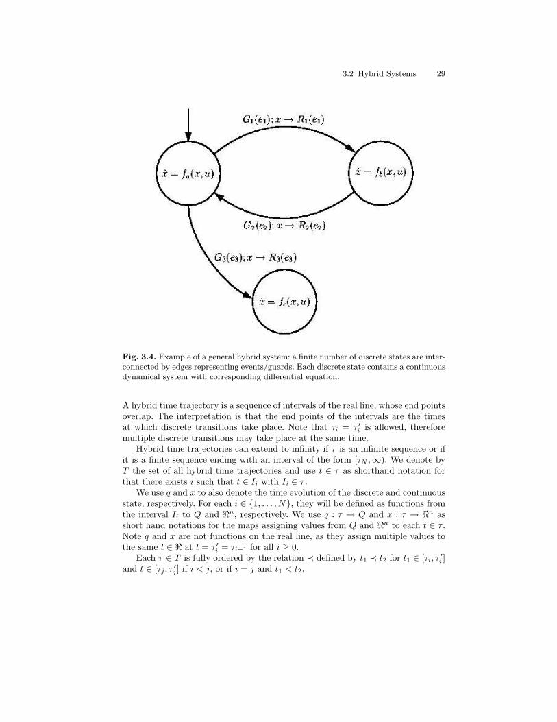
3.2 Hybrid Systems 29
Fig. 3.4. Example of a general hybrid system: a finite number of discrete states are inter-connected by edges representing events/guards. Each discrete state contains a continuousdynamical system with corresponding differential equation.
A hybrid time trajectory is a sequence of intervals of the real line, whose end pointsoverlap. The interpretation is that the end points of the intervals are the timesat which discrete transitions take place. Note that τi = τ ′i is allowed, thereforemultiple discrete transitions may take place at the same time.
Hybrid time trajectories can extend to infinity if τ is an infinite sequence or ifit is a finite sequence ending with an interval of the form [τN ,∞). We denote byT the set of all hybrid time trajectories and use t ∈ τ as shorthand notation forthat there exists i such that t ∈ Ii with Ii ∈ τ .
We use q and x to also denote the time evolution of the discrete and continuousstate, respectively. For each i ∈ 1, . . . , N, they will be defined as functions fromthe interval Ii to Q and <n, respectively. We use q : τ → Q and x : τ → <n asshort hand notations for the maps assigning values from Q and <n to each t ∈ τ .Note q and x are not functions on the real line, as they assign multiple values tothe same t ∈ < at t = τ ′i = τi+1 for all i ≥ 0.
Each τ ∈ T is fully ordered by the relation ≺ defined by t1 ≺ t2 for t1 ∈ [τi, τ ′i ]and t ∈ [τj , τ ′j ] if i < j, or if i = j and t1 < t2.
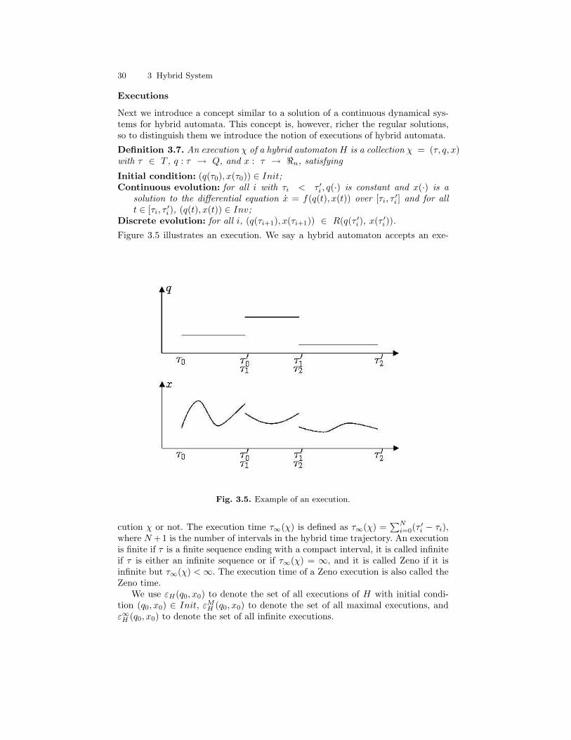
30 3 Hybrid System
Executions
Next we introduce a concept similar to a solution of a continuous dynamical sys-tems for hybrid automata. This concept is, however, richer the regular solutions,so to distinguish them we introduce the notion of executions of hybrid automata.
Definition 3.7. An execution χ of a hybrid automaton H is a collection χ = (τ, q, x)with τ ∈ T , q : τ → Q, and x : τ → <n, satisfying
Initial condition: (q(τ0), x(τ0)) ∈ Init;Continuous evolution: for all i with τi < τ ′i , q(·) is constant and x(·) is a
solution to the differential equation x = f(q(t), x(t)) over [τi, τ ′i ] and for allt ∈ [τi, τ ′i), (q(t), x(t)) ∈ Inv;
Discrete evolution: for all i, (q(τi+1), x(τi+1)) ∈ R(q(τ ′i), x(τ′i)).
Figure 3.5 illustrates an execution. We say a hybrid automaton accepts an exe-
Fig. 3.5. Example of an execution.
cution χ or not. The execution time τ∞(χ) is defined as τ∞(χ) =∑Ni=0(τ
′i − τi),
where N +1 is the number of intervals in the hybrid time trajectory. An executionis finite if τ is a finite sequence ending with a compact interval, it is called infiniteif τ is either an infinite sequence or if τ∞(χ) = ∞, and it is called Zeno if it isinfinite but τ∞(χ) <∞. The execution time of a Zeno execution is also called theZeno time.
We use εH(q0, x0) to denote the set of all executions of H with initial condi-tion (q0, x0) ∈ Init, εMH (q0, x0) to denote the set of all maximal executions, andε∞H (q0, x0) to denote the set of all infinite executions.
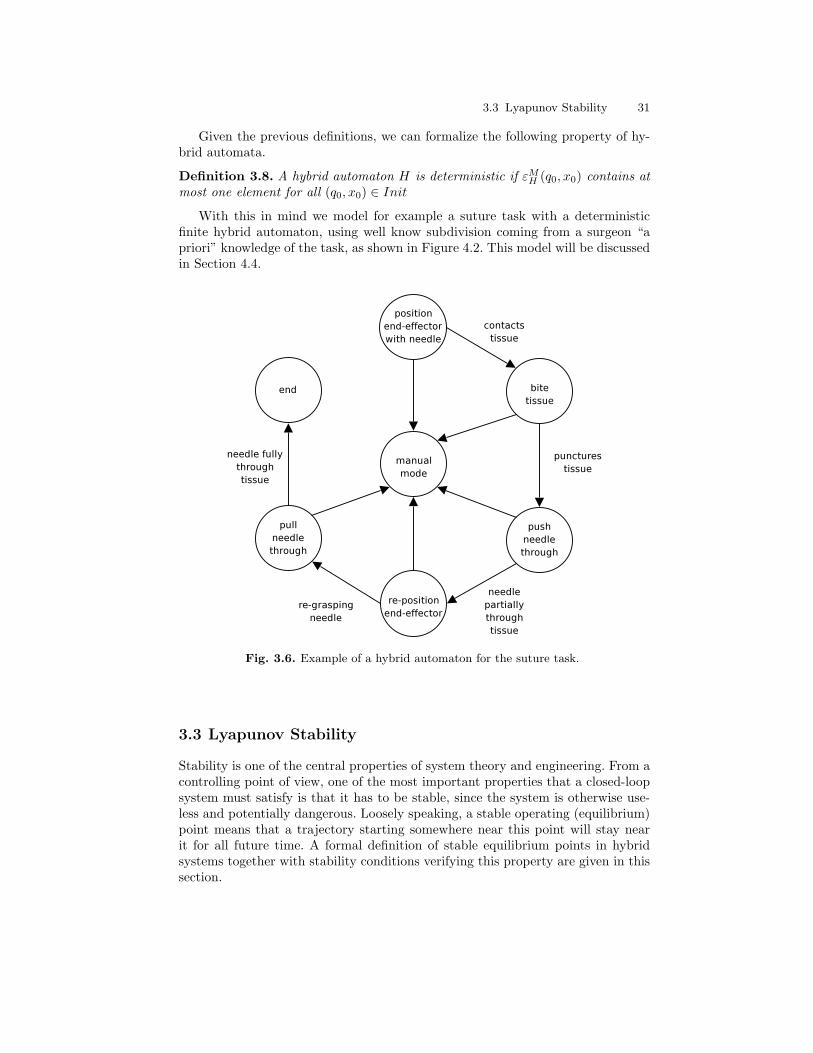
3.3 Lyapunov Stability 31
Given the previous definitions, we can formalize the following property of hy-brid automata.
Definition 3.8. A hybrid automaton H is deterministic if εMH (q0, x0) contains atmost one element for all (q0, x0) ∈ Init
With this in mind we model for example a suture task with a deterministicfinite hybrid automaton, using well know subdivision coming from a surgeon “apriori” knowledge of the task, as shown in Figure 4.2. This model will be discussedin Section 4.4.
Fig. 3.6. Example of a hybrid automaton for the suture task.
3.3 Lyapunov Stability
Stability is one of the central properties of system theory and engineering. From acontrolling point of view, one of the most important properties that a closed-loopsystem must satisfy is that it has to be stable, since the system is otherwise use-less and potentially dangerous. Loosely speaking, a stable operating (equilibrium)point means that a trajectory starting somewhere near this point will stay nearit for all future time. A formal definition of stable equilibrium points in hybridsystems together with stability conditions verifying this property are given in thissection.
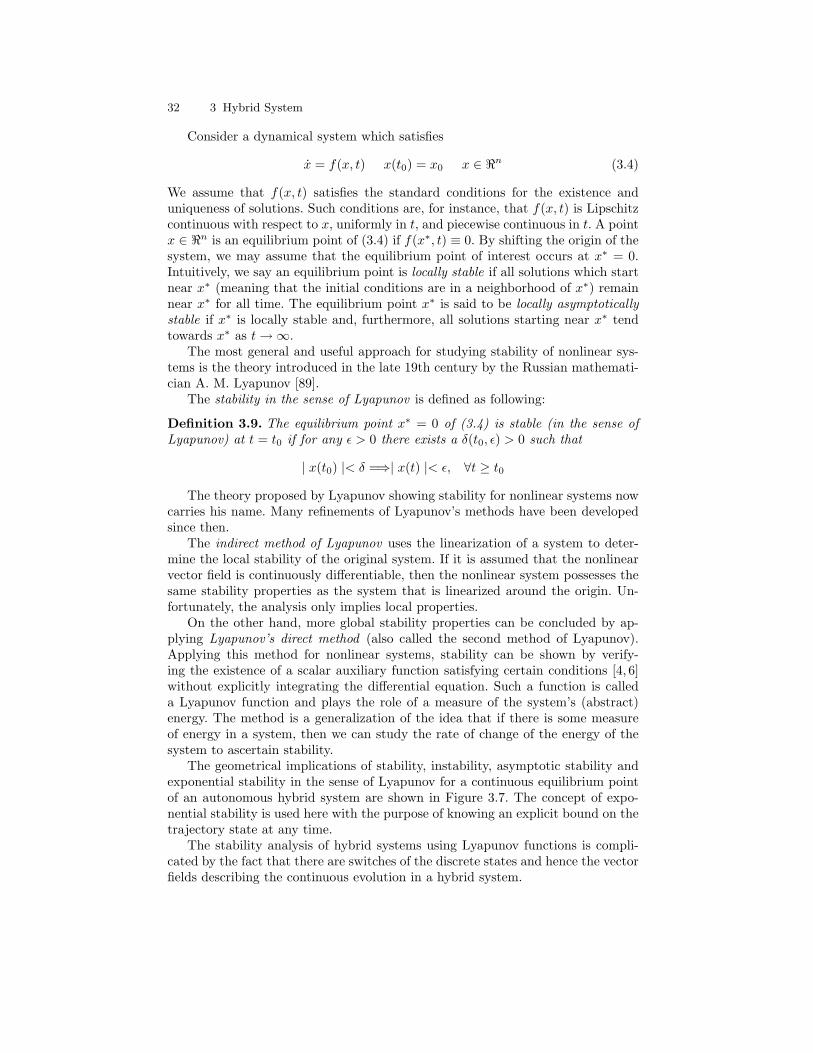
32 3 Hybrid System
Consider a dynamical system which satisfies
x = f(x, t) x(t0) = x0 x ∈ <n (3.4)
We assume that f(x, t) satisfies the standard conditions for the existence anduniqueness of solutions. Such conditions are, for instance, that f(x, t) is Lipschitzcontinuous with respect to x, uniformly in t, and piecewise continuous in t. A pointx ∈ <n is an equilibrium point of (3.4) if f(x∗, t) ≡ 0. By shifting the origin of thesystem, we may assume that the equilibrium point of interest occurs at x∗ = 0.Intuitively, we say an equilibrium point is locally stable if all solutions which startnear x∗ (meaning that the initial conditions are in a neighborhood of x∗) remainnear x∗ for all time. The equilibrium point x∗ is said to be locally asymptoticallystable if x∗ is locally stable and, furthermore, all solutions starting near x∗ tendtowards x∗ as t→∞.
The most general and useful approach for studying stability of nonlinear sys-tems is the theory introduced in the late 19th century by the Russian mathemati-cian A. M. Lyapunov [89].
The stability in the sense of Lyapunov is defined as following:
Definition 3.9. The equilibrium point x∗ = 0 of (3.4) is stable (in the sense ofLyapunov) at t = t0 if for any ε > 0 there exists a δ(t0, ε) > 0 such that
| x(t0) |< δ =⇒| x(t) |< ε, ∀t ≥ t0
The theory proposed by Lyapunov showing stability for nonlinear systems nowcarries his name. Many refinements of Lyapunov’s methods have been developedsince then.
The indirect method of Lyapunov uses the linearization of a system to deter-mine the local stability of the original system. If it is assumed that the nonlinearvector field is continuously differentiable, then the nonlinear system possesses thesame stability properties as the system that is linearized around the origin. Un-fortunately, the analysis only implies local properties.
On the other hand, more global stability properties can be concluded by ap-plying Lyapunov’s direct method (also called the second method of Lyapunov).Applying this method for nonlinear systems, stability can be shown by verify-ing the existence of a scalar auxiliary function satisfying certain conditions [4, 6]without explicitly integrating the differential equation. Such a function is calleda Lyapunov function and plays the role of a measure of the system’s (abstract)energy. The method is a generalization of the idea that if there is some measureof energy in a system, then we can study the rate of change of the energy of thesystem to ascertain stability.
The geometrical implications of stability, instability, asymptotic stability andexponential stability in the sense of Lyapunov for a continuous equilibrium pointof an autonomous hybrid system are shown in Figure 3.7. The concept of expo-nential stability is used here with the purpose of knowing an explicit bound on thetrajectory state at any time.
The stability analysis of hybrid systems using Lyapunov functions is compli-cated by the fact that there are switches of the discrete states and hence the vectorfields describing the continuous evolution in a hybrid system.
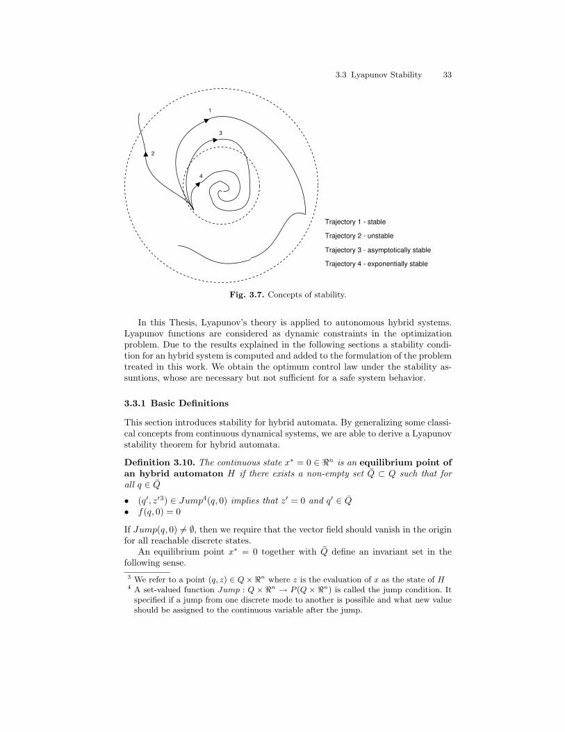
3.3 Lyapunov Stability 33
2
1
3
4
Trajectory 1 - stable
Trajectory 2 - unstable
Trajectory 3 - asymptotically stable
Trajectory 4 - exponentially stable
Fig. 3.7. Concepts of stability.
In this Thesis, Lyapunov’s theory is applied to autonomous hybrid systems.Lyapunov functions are considered as dynamic constraints in the optimizationproblem. Due to the results explained in the following sections a stability condi-tion for an hybrid system is computed and added to the formulation of the problemtreated in this work. We obtain the optimum control law under the stability as-suntions, whose are necessary but not sufficient for a safe system behavior.
3.3.1 Basic Definitions
This section introduces stability for hybrid automata. By generalizing some classi-cal concepts from continuous dynamical systems, we are able to derive a Lyapunovstability theorem for hybrid automata.
Definition 3.10. The continuous state x∗ = 0 ∈ <n is an equilibrium point ofan hybrid automaton H if there exists a non-empty set Q ⊂ Q such that forall q ∈ Q
• (q′, z′3) ∈ Jump4(q, 0) implies that z′ = 0 and q′ ∈ Q• f(q, 0) = 0
If Jump(q, 0) 6= ∅, then we require that the vector field should vanish in the originfor all reachable discrete states.
An equilibrium point x∗ = 0 together with Q define an invariant set in thefollowing sense.3 We refer to a point (q, z) ∈ Q×<n where z is the evaluation of x as the state of H4 A set-valued function Jump : Q × <n → P (Q × <n) is called the jump condition. It
specified if a jump from one discrete mode to another is possible and what new valueshould be assigned to the continuous variable after the jump.

34 3 Hybrid System
Definition 3.11. A set M ⊂ Init is called invariant if for all (q0, x0) ∈ M ,(τ, q, x) ∈ εH(q0, x0), and t ∈ τ , it holds that (q(t), x(t)) ∈M .
We can now define the notion of stability and enunciate the Lyapunov’s StabilityTheorem for Hybrid Automata.
Definition 3.12. Assume x∗ = 0 is an equilibrium point of a hybrid automatonH. It is called stable, if for all ε > 0 there exists δ > 0 such that for all executionsχ = (τ, x, q) ∈ εH(q0, x0) with ‖x0‖ < δ it holds that ‖x(t)‖ < ε for all t ∈ τ .
The equilibrium point x∗ = 0 is asymptotically stable if it is stable andδ < 0 can be chosen such that for all executions χ = (τ, x, q) ∈ ε∞H (q0, x0) with‖x0‖ < δ it holds that limt→τ∞‖x(t)‖ = 0.
Note that in the definition of stability , the discrete state of hybrid automataare not taken into account. This means that an equilibrium point of a hybridautomaton is considered asymptotically stable, although the discrete evolutionnot converge.
Theorem 3.13. Consider a hybrid automaton H, such that (q, z) ∈ Q × <n and(q′, z′) ∈ Jump(q, z) imply that z′ = z. Assume there exists an open set Ω ⊂Q × <n, such that (q, 0) ∈ Ω for some q ∈ Q and that x∗ = 0 is an equilibriumpoint of H. Let V : Ω → < be a continuously differentiable function in its secondargument such that for all q ∈ Q
• V (q, 0) = 0• V (q, x) > 0,∀x, (q, x) ∈ Ω\0• ∂V
∂x f(q, x) ≤ 0,∀x, (q, x) ∈ Ω
If for all χ = (τ, q, x) ∈ εH(q0, x0) with (q0, x0) ∈ Init ∩Ω and for all q ∈ Q, thesequence V (q(τi), x(τi)) : q(τi) = q is non-increasing (or empty), then x∗ = 0 isstable.
Theorem 3.13 gives sufficient conditions for the stability of the origin of asystem. It does not, however, give a prescription for determining the Lyapunovfunction V (q, x). Since the theorem only gives sufficient conditions, the search for aLyapunov function establishing stability of an equilibrium point could be arduous.However, it is a remarkable fact that the converse of Theorem 3.13 also exists: ifan equilibrium point is stable, then there exists a function V (q, x) satisfying theconditions of the theorem. However, the utility of this and other converse theoremsis limited by the lack of a computable technique for generating Lyapunov functions.Theorem 3.13 also stops short of giving explicit rates of convergence of solutionsto the equilibrium. It may be modified to do so in the case of exponentially stableequilibria.
3.3.2 Existing stability results
There exist several results in the literature using Lyapunov theory to show stabilityfor hybrid systems and to illustrate that stability of hybrid systems in generaldepends on the switchings of discrete states and corresponding vector fields. Thepurpose of this section is to present some of these.

3.3 Lyapunov Stability 35
Peletis-DeCarlo An early theorem guaranteeing (asymptotic) stability of linearhybrid systems is proposed in [142] by Peletis and DeCarlo. It is assumedthat the time between vector field switchings is bounded above and below bysome constant, implying that an infinite number of switching cannot occur infinite time but there will be an infinite number of switching when time goes toinfinity. By introducing multiple Lyapunov functions, one Lyapunov functionVi for each linear vector field fi, which are positive definite and continuouslydifferentiable (and hence continuous), (asymptotic) stability is guaranteed byrequiring the energy at the consecutive times (just before switching) to be adecreasing sequence, as shown in Figure 3.8. When there are switchings toanother linear vector field at the times t1, t2 and so on, the values of thecorresponding Lyapunov function just before the switchings are marked byfilled circles. The sequence of consecutive values marked by the circles mustbe (strictly) decreasing according to the (asymptotic) stability result.
V
tt0 t1 t2 t3 t4 t5 t6
V1
V2
V1
V3
V2 V3
V1
Fig. 3.8. Illustration of the decrease of energy in the (asymptotic) stability result ofPeleties-DeCarlo.
Dogruel-Ozguner Another proposed (asymptotic) stability result for hybrid sys-tems is the theorem presented in [78] by Dogruel and Ozguner. It is appliedto hybrid systems with nonlinear vector fields, where possible sliding modeshave been replaced by an equivalent continuous dynamics in such a way thatthe system spends equal time in each of the discrete states involved in theswitchings. It is assumed that the origin is an equilibrium point for all vectorfields. By introducing a common Lyapunov function which is positive definiteand continuously differentiable (and hence continuous), (asymptotic) stabil-ity is guaranteed by requiring the energy to be decreasing all the time for allvector fields that are possible in a certain region, as shown in Figure 3.9.
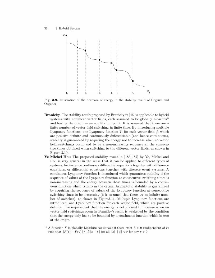
36 3 Hybrid System
V
tt0 t1 t2 t3 t4 t5 t6
Fig. 3.9. Illustration of the decrease of energy in the stability result of Dogruel andOzguner
Branicky The stability result proposed by Branicky in [46] is applicable to hybridsystems with nonlinear vector fields, each assumed to be globally Lipschitz5
and having the origin as an equilibrium point. It is assumed that there are afinite number of vector field switching in finite time. By introducing multipleLyapunov functions, one Lyapunov function Vi for each vector field fi whichare positive definite and continuously differentiable (and hence continuous),stability is guaranteed by requiring the energy not to increase when no vectorfield switchings occur and to be a non-increasing sequence at the consecu-tive times obtained when switching to the different vector fields, as shown inFigure 3.10.
Ye-Michel-Hou The proposed stability result in [186, 187] by Ye, Michel andHou is very general in the sense that it can be applied to different types ofsystems, for instance continuous differential equations together with differenceequations, or differential equations together with discrete event systems. Acontinuous Lyapunov function is introduced which guarantees stability if thesequence of values of the Lyapunov function at consecutive switching times isnon-increasing and the energy between these times is bounded by a contin-uous function which is zero in the origin. Asymptotic stability is guaranteedby requiring the sequence of values of the Lyapunov function at consecutiveswitching times to be decreasing (it is assumed that there are an infinite num-ber of switches), as shown in Figure3.11. Multiple Lyapunov functions areintroduced, one Lyapunov function for each vector field, which are positivedefinite. The requirement that the energy is not allowed to increase when novector field switchings occur in Branicky’s result is weakened by the conditionthat the energy only has to be bounded by a continuous function which is zeroat the origin.
5 A function F is globally Lipschitz continuous if there exist L > 0 (indipendent of r)such that ‖F (z)− F (y)‖ ≤ L‖z − y‖ for all ‖z‖, ‖y‖ < r for any r > 0
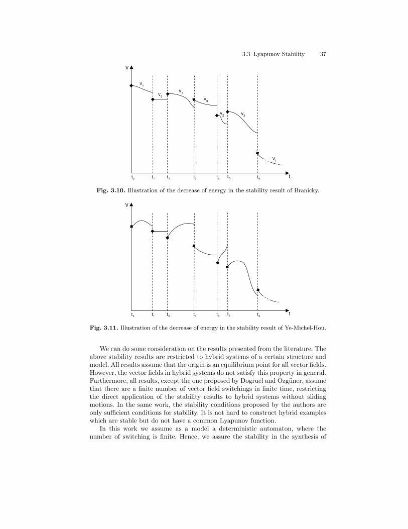
3.3 Lyapunov Stability 37
V
tt0 t1 t2 t3 t4 t5 t6
V1
V2
V1
V3
V2 V3
V1
Fig. 3.10. Illustration of the decrease of energy in the stability result of Branicky.
V
tt0 t1 t2 t3 t4 t5 t6
Fig. 3.11. Illustration of the decrease of energy in the stability result of Ye-Michel-Hou.
We can do some consideration on the results presented from the literature. Theabove stability results are restricted to hybrid systems of a certain structure andmodel. All results assume that the origin is an equilibrium point for all vector fields.However, the vector fields in hybrid systems do not satisfy this property in general.Furthermore, all results, except the one proposed by Dogruel and Ozguner, assumethat there are a finite number of vector field switchings in finite time, restrictingthe direct application of the stability results to hybrid systems without slidingmotions. In the same work, the stability conditions proposed by the authors areonly sufficient conditions for stability. It is not hard to construct hybrid exampleswhich are stable but do not have a common Lyapunov function.
In this work we assume as a model a deterministic automaton, where thenumber of switching is finite. Hence, we assure the stability in the synthesis of
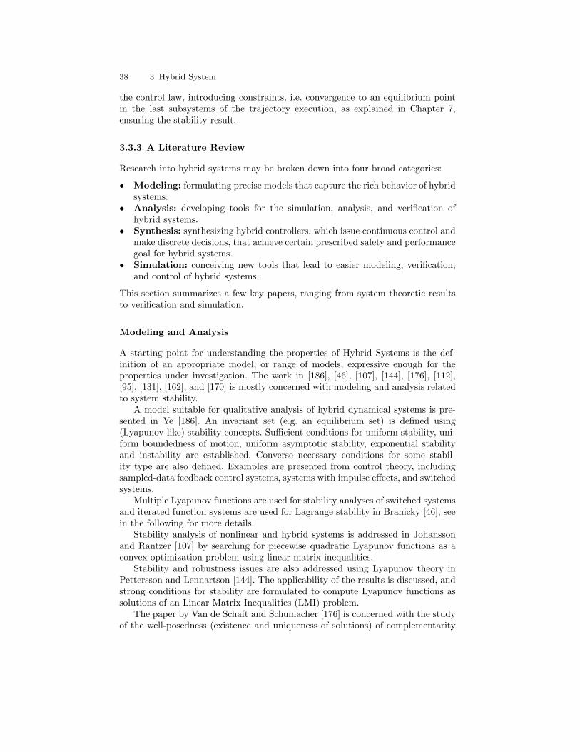
38 3 Hybrid System
the control law, introducing constraints, i.e. convergence to an equilibrium pointin the last subsystems of the trajectory execution, as explained in Chapter 7,ensuring the stability result.
3.3.3 A Literature Review
Research into hybrid systems may be broken down into four broad categories:
• Modeling: formulating precise models that capture the rich behavior of hybridsystems.
• Analysis: developing tools for the simulation, analysis, and verification ofhybrid systems.
• Synthesis: synthesizing hybrid controllers, which issue continuous control andmake discrete decisions, that achieve certain prescribed safety and performancegoal for hybrid systems.
• Simulation: conceiving new tools that lead to easier modeling, verification,and control of hybrid systems.
This section summarizes a few key papers, ranging from system theoretic resultsto verification and simulation.
Modeling and Analysis
A starting point for understanding the properties of Hybrid Systems is the def-inition of an appropriate model, or range of models, expressive enough for theproperties under investigation. The work in [186], [46], [107], [144], [176], [112],[95], [131], [162], and [170] is mostly concerned with modeling and analysis relatedto system stability.
A model suitable for qualitative analysis of hybrid dynamical systems is pre-sented in Ye [186]. An invariant set (e.g. an equilibrium set) is defined using(Lyapunov-like) stability concepts. Sufficient conditions for uniform stability, uni-form boundedness of motion, uniform asymptotic stability, exponential stabilityand instability are established. Converse necessary conditions for some stabil-ity type are also defined. Examples are presented from control theory, includingsampled-data feedback control systems, systems with impulse effects, and switchedsystems.
Multiple Lyapunov functions are used for stability analyses of switched systemsand iterated function systems are used for Lagrange stability in Branicky [46], seein the following for more details.
Stability analysis of nonlinear and hybrid systems is addressed in Johanssonand Rantzer [107] by searching for piecewise quadratic Lyapunov functions as aconvex optimization problem using linear matrix inequalities.
Stability and robustness issues are also addressed using Lyapunov theory inPettersson and Lennartson [144]. The applicability of the results is discussed, andstrong conditions for stability are formulated to compute Lyapunov functions assolutions of an Linear Matrix Inequalities (LMI) problem.
The paper by Van de Schaft and Schumacher [176] is concerned with the studyof the well-posedness (existence and uniqueness of solutions) of complementarity
3.3 Lyapunov Stability 39
systems, special hybrid systems that are related to the linear complementary prob-lem of mathematical programming. Complementarity modeling is presented first,and well-posedness is defined. The paper, then establishes sufficient conditions forthe uniqueness of smooth continuations of complementary systems of arbitrarynumber of discrete states.
Feedback stabilization of a class on nonlinear systems using hybrid feedbackcontrollers is addressed by Kolmanovsky and McClamroch [112]. The authorsstudy the general structure of systems represented as a cascade of a linear timeinvariant and a nonlinear system. The controller is constructed to induce a slowand a fast dynamics, and feedback control linearizes the original nonlinear systemat the two different time scales.
The domain of attraction of a nonlinear control systems is expanded by Guck-enheimer [95] and McClarmroch [131] using switching. The resulting nonlinearcontrol system admits a family of equilibria corresponding to constant control in-puts. Switching occurs at discrete times from one control input to another so thatthe system gradually progresses from one equilibrium point to another towards afinal equilibrium.
A Discrete Event System (DES) automaton is used in Stiver [162] to describe acontinuous plant, its discrete event controller, and the interface and the completesystem is analyzed as a hybrid control system. The system is proved to be adeterministic and controllable hybrid system for which a controller design methodis proposed. To extend this approach, invariant based methods for control designare also presented. This method is based on the natural invariants of the continuouspart and has appeared in [161].
The control design of a class of hybrid systems with continuous dynamic de-scribed by pure integrators is studied by Tittus and Egardt in [170]. This classincludes a small set of hybrid systems, but it models the important class of con-trol batch processes. The notion of controllability for this class is proposed and acontrollability analysis formulated as a backward reachability problem is derived.The analysis is based on a hybrid automaton model, which includes a hybrid plantand a hybrid controller that interact in a feedback loop.
Synthesis
The design of controllers suitable for hybrid systems, or based on hybrid systemtheory, is address in papers [149], [67], [56], [139], [126], [123].
The paper by Raisch and O’Young [149] addresses the problem of a continuousplant controlled via symbolic feedback. The hybrid problem is first translatedinto a purely discrete problem by approximating the continuous plant model by anon deterministic finite state machine. Past measurements and control symbols areused to improve approximation accuracy and adjusted it to required specifications.An optimal controller enforcing the specifications is then computed by applyingsupervisory control theory.
Supervisory control for a class of continuous-time hybrid systems is studiedby Cury [67]. The supervisor is allowed to switch the discrete-valued input signalwhen threshold events are observed. The objective of the control is to synthesize anonblocking supervisor that keeps the set of possible control sequences and thresh-old events for the closed-loop system between given upper and lower bounds in the
40 3 Hybrid System
sense of set containment. The paper shows that this problem can be converted intoa supervisor synthesis problem for a DES. A finite representation may not existfor the exact DES model of the hybrid system, however. The algorithm bypassesthis difficulty by constructing finite-state Muller automata that accept outer ap-proximations to the exact controlled threshold-event language is presented. Thepaper shows that supervisors synthesized for the approximating automata are ableto achieve the original specifications when applied to the true hybrid system.
Hierarchical hybrid control systems are defined by Caines and Wei [56] usingthe notion of dynamic consistency. This notion is extended to hybrid systems bydefining a set of dynamically consistent hybrid partition machines, with between-block and in-block controllability properties. The hybrid partition machines areorganized in a lattice structure, whose properties are investigated.
Nerode and Kohn [139] propose a Multiple Agent Hybrid Control Architec-ture to implement a real-time distributed software controller. The architecture isbased on principles of declarative control, concurrent programming and dynami-cal hybrid systems. Each agent computes its control action by solving a relaxedconvex optimization problem. An evolution of this approach is proposed in (Kohnet al., 1998) by finding an unbiased estimate of the plant state given dynamic andnoisy measurements represented in a multiplicity of forms, without converting alldata to a common representation. The paper defines the Multiple Agent HybridEstimation Architecture to allow hetereogenous data to flow between individualagents in the network and to improve their individual capability of estimating thecurrent plant state.
Hybrid control of large scale, multiagent systems based on optimal control andgame theory is addressed by Lygeros, Godbole and Sastry [126]. The hybrid designis seen as a game between two players: the control, which is chosen by the designer,and noise including the actions of other agents, and unmodeled environmentaldisturbances. The two players compete over cost functions that encode propertiesthat the closed loop hybrid system needs to satisfy, e.g. safety. The control ”wins”the game if it can keep the system safe for any allowable disturbance. The gametheoretical methodology is used to compute the continuous controllers as well asthe sets of safe states where the control ”wins” the game. The sets of safe statesare used to construct an interface to the discrete domain that guarantees the safeoperation of the combined hybrid system. This approach has been used in airtraffic management [172] and in control of automated highway systems [127].
The integration of timed automata and robust control methods for the controlof complex dynamical systems is analyzed by Lemmon and Antsaklis [123]. Recentresults from computer science and robust control are presented and integrationguidelines are given to study stability and boundedness conditions of switchedsystems. Robust control methods have also been used for hybrid control [16,17].
Simulation
Papers on simulation and performance verification are the final group of this briefsummary of theoretical aspects of Hybrid Systems, and include [12], [16], [104], [73].Here a most relevant distinction is that between using timed automata and hybridautomata.
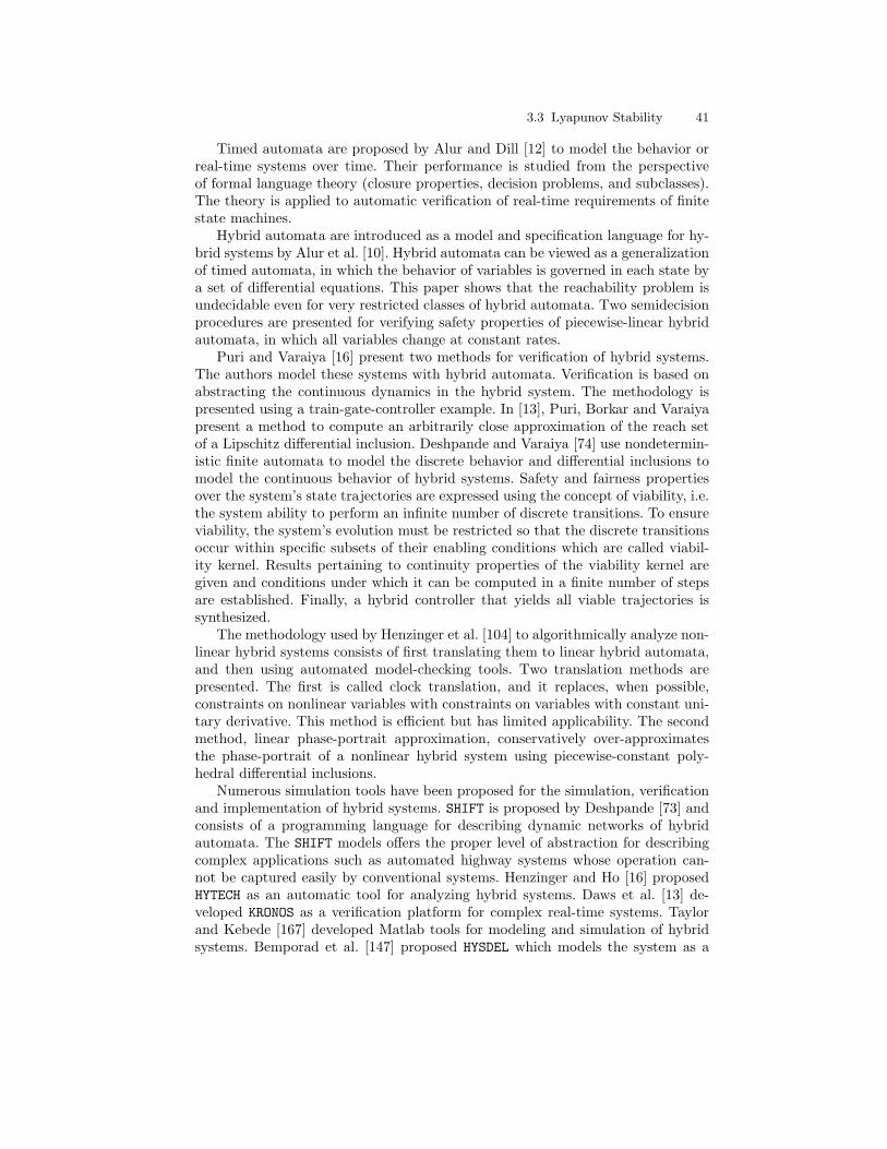
3.3 Lyapunov Stability 41
Timed automata are proposed by Alur and Dill [12] to model the behavior orreal-time systems over time. Their performance is studied from the perspectiveof formal language theory (closure properties, decision problems, and subclasses).The theory is applied to automatic verification of real-time requirements of finitestate machines.
Hybrid automata are introduced as a model and specification language for hy-brid systems by Alur et al. [10]. Hybrid automata can be viewed as a generalizationof timed automata, in which the behavior of variables is governed in each state bya set of differential equations. This paper shows that the reachability problem isundecidable even for very restricted classes of hybrid automata. Two semidecisionprocedures are presented for verifying safety properties of piecewise-linear hybridautomata, in which all variables change at constant rates.
Puri and Varaiya [16] present two methods for verification of hybrid systems.The authors model these systems with hybrid automata. Verification is based onabstracting the continuous dynamics in the hybrid system. The methodology ispresented using a train-gate-controller example. In [13], Puri, Borkar and Varaiyapresent a method to compute an arbitrarily close approximation of the reach setof a Lipschitz differential inclusion. Deshpande and Varaiya [74] use nondetermin-istic finite automata to model the discrete behavior and differential inclusions tomodel the continuous behavior of hybrid systems. Safety and fairness propertiesover the system’s state trajectories are expressed using the concept of viability, i.e.the system ability to perform an infinite number of discrete transitions. To ensureviability, the system’s evolution must be restricted so that the discrete transitionsoccur within specific subsets of their enabling conditions which are called viabil-ity kernel. Results pertaining to continuity properties of the viability kernel aregiven and conditions under which it can be computed in a finite number of stepsare established. Finally, a hybrid controller that yields all viable trajectories issynthesized.
The methodology used by Henzinger et al. [104] to algorithmically analyze non-linear hybrid systems consists of first translating them to linear hybrid automata,and then using automated model-checking tools. Two translation methods arepresented. The first is called clock translation, and it replaces, when possible,constraints on nonlinear variables with constraints on variables with constant uni-tary derivative. This method is efficient but has limited applicability. The secondmethod, linear phase-portrait approximation, conservatively over-approximatesthe phase-portrait of a nonlinear hybrid system using piecewise-constant poly-hedral differential inclusions.
Numerous simulation tools have been proposed for the simulation, verificationand implementation of hybrid systems. SHIFT is proposed by Deshpande [73] andconsists of a programming language for describing dynamic networks of hybridautomata. The SHIFT models offers the proper level of abstraction for describingcomplex applications such as automated highway systems whose operation can-not be captured easily by conventional systems. Henzinger and Ho [16] proposedHYTECH as an automatic tool for analyzing hybrid systems. Daws et al. [13] de-veloped KRONOS as a verification platform for complex real-time systems. Taylorand Kebede [167] developed Matlab tools for modeling and simulation of hybridsystems. Bemporad et al. [147] proposed HYSDEL which models the system as a
42 3 Hybrid System
discrete hybrid automaton (DHA) using the high level modeling language HYSDEL(HYbrid System DEscription Language). Such a model can be later translatedinto Mixed Integer Dynamical (MLD) modeling framework. Other computer sim-ulation and verification tools that are (also) used for hybrid systems are BaSiP,Modelica, Chi, 20-sim, UPPAAL, and many others. Simulation models can rep-resent the plant with a high degree of detail, providing a close correspondencebetween simulated behavior and real plant behavior. This approach is, for anylarge system, computationally very demanding, and moreover it is difficult to un-derstand from a simulation how the behavior depends on model parameters. Thisdifficulty is even more pronounced in the case of large hybrid systems which con-sist of many interacting modules. Fast simulation techniques based on variancereduction, and perturbation analysis techniques [5] have been developed in orderto partially overcome these limitations.
3.4 Conclusions
In this chapter an overview on hybrid system framework is presented. Becausethe literature on hybrid systems is broad and covers many areas in engineeringand computer science, here we present only some aspects strictly related to thisresearch. We define a hybrid automaton, that is the model that we choose todescribe our task. We summarized the state of the art on the analysis of hybridsystems with emphasis on the stability results and some consideration on synthesisand simulation. We use the concepts and definitions summarized here as the baseto set up the approach presented in the following chapters.
4
Robotic Surgery
The more a machine is developed the more it disappears.Jose Maria Galvan
Surgical theaters are changing rapidly. Also surgical techniques are changing.Minimally Invasive Surgery (MIS) has already been introduced some time ago.After the introduction of MIS, computers and computer controlled surgical toolswere more and more integrated into the surgical theater. The next step was tointroduce the robot for surgical purposes. In the future surgeons will not evenhave to touch the patient while operating.
To understand the problems that arise when the new robotic techniques isintroduced, an introduction to medical robotics is given in this Section. The terms’minimally invasive surgery’ and ’microsurgery’ are introduced. Their advantages,disadvantages and shortcomings are discussed. The most important advantages arefast recovery and less pain for the patient. The most important disadvantages arethe less ergonomic situation for the surgeon and the bad visibility of the operationarea. A difference is made between ’robotic surgery’ and ’computer aided surgery’(CAS). CAS system is powered by the surgeon, while a medical robot is not.Medical robots can be divided in four groups, (i) passive robots, (ii) active robots,(iii) synergistic systems and (iv) master-slave systems. Especially master-slavesystems seem to be very promising to use on large scale, because they are able tohandle soft tissues and can be used for a large range of operations.
As stated, robots seem to be very promising for use during surgery. However,a lot of aspects have to be improved to increase their performance, not only withrespect to mechanical design, but also with respect to control and sensing. Besidesthese technical aspects also clinical and social aspects play a role. Questions suchas: ’Is the result of robotic surgery really better than the result of conventionalsurgery? Is such a big investment worthwhile? Are there any surgeons who areable and willing to handle such a robot?’ arise.
Many studies were carried out in order to introduce new robotic techniques orsimply to improve the existing ones. In the literature studies on decomposition ofcomplex task, especially surgical task, have the objective to develop simulators forevaluating surgical skill. Few works address the problem of automatic execution
44 4 Robotic Surgery
of surgical task, which requires the identification of an underlying mental modelto derive a possible task control sequence. The model aims at analyzing and seg-menting the task in simpler sub-tasks. As an example of surgical task at the endof this Chapter we consider suture, which is well defined and parametric in nature.This approach generates a model, hybrid automaton, where the states are basicskills and the transitions between states are governed by knowledge of the taskand issues of good performance with respect to a given task.
In this Chapter we will summarize the main aspects of the research area towhich this Thesis contributes. In Section 4.1 some definitions of medical aspectsare presented, in Section 4.2 attention is given to clinical and social aspects ofrobot surgery. In Section 4.3, we introduce segmentation as a technique widelyused to subdivide and analyze task. In Section 4.4 we describe the surgical taskthat we have been using in this work, as representative task of the spectrum ofsurgical procedures.
4.1 Medical Aspects
Minimally Invasive Surgery
As long as operations exist, procedures are developed to decrease the size of thesurgical incision. Smaller incisions lead to less trauma and less pain for the patient.This results in a faster recovery of the patient. Patients can return earlier to theirhomes and freeing place for other patients. Beside the advantages for the patientscare, a fast recovery of the patient has also several economical advantages, e.g.lower medical costs and the patient is able to return earlier to work. The searchfor smaller incisions has led to minimally invasive surgery. The small incisions ofMIS are used to introduce special instruments with a long rod transmission mecha-nism through a cannula into the body of the patient. By using a small camera, thesurgeon is able to follow the progress of the operation on a screen. The term min-imally invasive surgery covers all surgery with small incisions and endoscopes likethorascopy (chest cavity), arthroscopy (joints), laparoscopy (abdominal cavity),pelviscopy (pelvis) and angioscopy (bloodvessels).
Although MIS fastens the rehabilitation of the patients, it also has some dis-advantages. In open surgery the surgeon has more space and freedom to move ina large operation area. With MIS, the operation area is smaller and the freedomto move the operation tool decreases with the use of an endoscope. Laparoscopictools are long and have only four degrees of freedom. These four degrees of free-dom include rotation around and translation along the axis perpendicular to theincision surface, and rotation around the two axes on the incision surface, as shownin Figure 4.1. Because of the long instruments the operative situation is less er-gonomic for the surgeon. It takes more energy to use the laparoscopic tools becauseof the rod transmission between the surgeons hands and the tip of the instruments.Furthermore, the surgeon has to concentrate on the reverse motion direction ofhis hands and the tip of the instrument. For example, a motion to the right ofthe surgeon is followed by a motion to the left of the instrument tip. The surgeonhas to develop more skills to perform the same operation than without MIS tech-niques. Another disadvantage of MIS is the interaction between the surgeon and
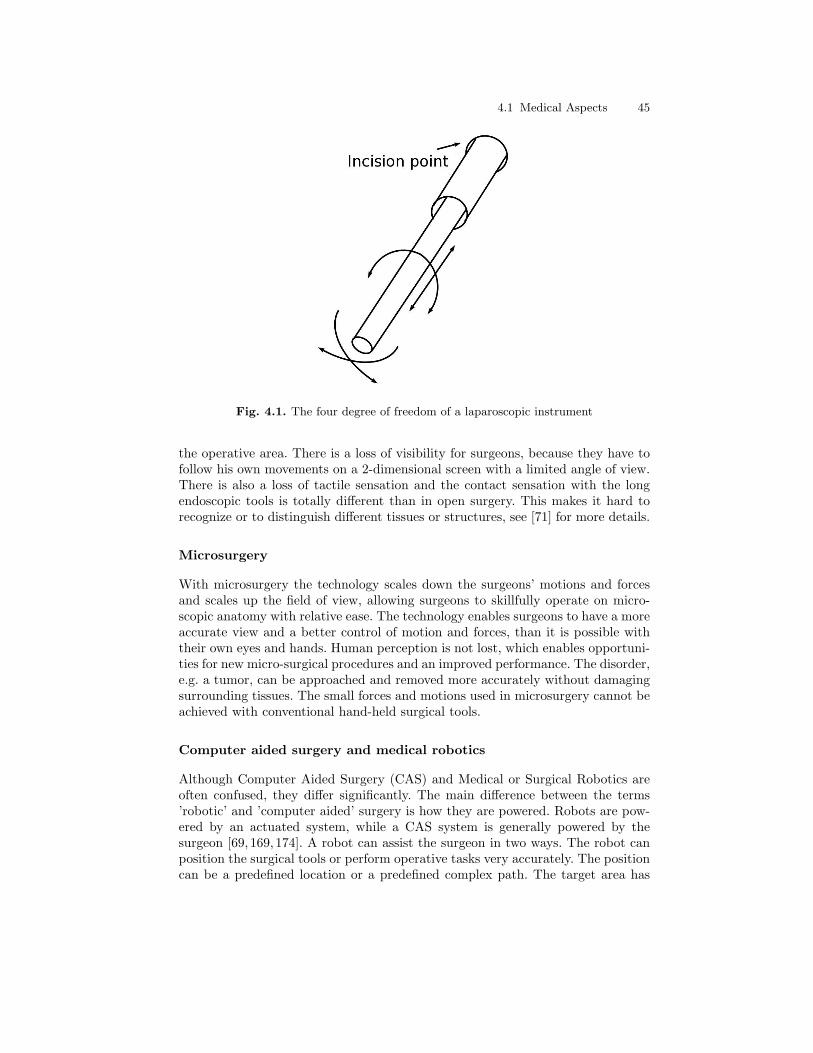
4.1 Medical Aspects 45
Fig. 4.1. The four degree of freedom of a laparoscopic instrument
the operative area. There is a loss of visibility for surgeons, because they have tofollow his own movements on a 2-dimensional screen with a limited angle of view.There is also a loss of tactile sensation and the contact sensation with the longendoscopic tools is totally different than in open surgery. This makes it hard torecognize or to distinguish different tissues or structures, see [71] for more details.
Microsurgery
With microsurgery the technology scales down the surgeons’ motions and forcesand scales up the field of view, allowing surgeons to skillfully operate on micro-scopic anatomy with relative ease. The technology enables surgeons to have a moreaccurate view and a better control of motion and forces, than it is possible withtheir own eyes and hands. Human perception is not lost, which enables opportuni-ties for new micro-surgical procedures and an improved performance. The disorder,e.g. a tumor, can be approached and removed more accurately without damagingsurrounding tissues. The small forces and motions used in microsurgery cannot beachieved with conventional hand-held surgical tools.
Computer aided surgery and medical robotics
Although Computer Aided Surgery (CAS) and Medical or Surgical Robotics areoften confused, they differ significantly. The main difference between the terms’robotic’ and ’computer aided’ surgery is how they are powered. Robots are pow-ered by an actuated system, while a CAS system is generally powered by thesurgeon [69, 169, 174]. A robot can assist the surgeon in two ways. The robot canposition the surgical tools or perform operative tasks very accurately. The positioncan be a predefined location or a predefined complex path. The target area has
46 4 Robotic Surgery
to be defined very accurately, because the robot has to be programmed for itssurgical task. The target operation area is defined during the pre-operative phase.Both operations with medical robotics or with CAS systems use a pre-operativephase. With CAS systems the pre-operative phase is only used for simulating andplanning the operative procedure, programming of instruments is not necessary.Unexpected situations can be avoided and the operation time can be decreased.However, robots are able to provide a greater accuracy than CAS systems. Anotherreason why robots are superior to CAS systems is the ability to constrain the mo-tions of the system. A robotic system has a predefined safety concept, which doesnot change during operation. The movements of a CAS system are established bythe decisions of surgeons, who can change the operation plan every moment theywant. They can neglect warnings or cut into unsafe regions.
Robotic systems
Robots are used to improve the outcome of operations. Different kinds of surgicalrobots exists. It is possible to divide them in groups related to their operative func-tion or in groups related to the way they function. There exist (i) passive robots,(ii) active robots, (iii) synergistic systems and (iv) master-slave systems [69].
Passive robots are used as tool-holders and do not have an operative task. Theiradvantage is, that they do not get tired and keep tools accurately in position for along time. An active robot must be able to carry out more complex motions thenpassive robots. They have an operative task, which they perform autonomously.That is why most active robots are developed for one specific task within thetotal operation procedure. The safety demands are high for active robots. Someexamples of active robots are laparoscopic cameras or robots used for arthroscopy.Because arthroscopy (joints) deals with bones, the modeling and calibration phaseare easier than to deal with soft tissue.
The third group of medical robots contains the synergistic systems. Synergisticsystems are controlled by both the surgeon and a computer. The surgeon is ableto use the machine within a predefined motion and force region. Oppositely toactive robots, synergistic systems do not work autonomously. The operationaltask is performed by the surgeon, but the synergistic robot system constrains thesurgeon. This reduces the risk of failures without loosing the surgeons skills andjudgment.
The fourth group consists of the master-slave systems, also called teleopera-tion systems. Master-slave systems are also non-autonomous. At the master sidethere are the surgeon, the master robot and visual and haptic displays. The masterrobot is controlled by the surgeon. At the slave side there are the patient, the slaverobot, haptic sensors and cameras. The slave robot is in contact with the patientand follows the instructions of the master robot. In this way the slave robot per-forms the actual operation. The surgeon controls the master robot on the basis ofvisual feedback and, if present, haptic feedback from the operation area. Visualfeedback can either be two or three dimensional and is established with camerasat the operation area. The cameras are a part of the slave robot and, accordinglycan be controlled with the master robot. The slave robot can use instruments forconventional surgery, instruments for MIS, instruments for microsurgery or a com-bination of them. The big advantages of master- slave systems above active robots
4.2 Clinical and Social Aspects 47
is that they can handle with soft tissue and be used for several operative tasks,because the surgeon is in control of the master robot. The ergonomic situationof the surgeon improves when master-slave systems are used. They can performthe operation sitting at the console and does not have to hold the instruments fora long time at the same position. The master and the slave robot can be decou-pled. While the master robot is moved, the slave robot keeps holding its position.Although the distance between master and slave robot normally is a few meters,master-slave systems have the potential to be used in long distance tele-surgery. Inthat case the data transmission has to be fast because of time delays between themaster and the slave side. Master-slave systems have the potential to use motionand force scaling. Motion scaling has the advantage that the surgical tools can bepositioned very accurately. Also tremor of the surgeons hands can be filtered out.Force scaling can only be used if haptic feedback is present. Forces can be scaledupward from slave to master to let the surgeon have better notice of properties ofthe operation area. However, commercial systems at this moment lack the presenceof total haptic feedback.
A special group of master-slave systems are the surgical simulators. Surgicalsimulators are not used for surgical intervention, but as training facility for traineesor as operation planning facility. A surgical simulator has the same structure asthe master-slave system. Instead of a real patient and a real slave robot, a virtualpatient and a virtual slave robot are introduced by a computer. The computerproduces images of the operative area and computes force feedback for the masterrobot of the contact forces between organs and surgical instruments. The mo-tion images and contact forces are reproduced and displayed as they are in realsituations.
The main benefits of using robots for surgical applications are improved pre-cision, stability and dexterity. To take the patients and surgeons advantage ofthese benefits, improvements have to be made in mechanical design, sensing andcontrol [65,106].
4.2 Clinical and Social Aspects
The reason why robots integrate slower into the surgical theater than in industrialenvironments is not only due to technical aspects. The most important social as-pect is safety. The safety requirements for medical robots are a lot more stringentthan industrial robots. Safety of a system can be achieved by active and passivesafety mechanisms in the mechanical design of the system. Passive mechanismsinclude the materials used and passive joints. An example of an active mechanismis a switch that turns off the instrument when force or motion limits are exceeded.Safety concepts can also be programmed into the software of the robot. Anotherpossibility to ensure safety is to keep the robot under supervision of the surgeon.Synergistic robots are good examples of this possibility. Another way is super-vision of the progress of the operation by surgeons on a screen, while they areable to stop the robot in an easy way. The startup times of most medical robots,especially master-slave systems, is quite long, sometimes up to fifteen minutes.Every time the system is stopped for safety reasons, it takes another quarter of an
48 4 Robotic Surgery
hour to continue the operation. Robots will only be used for operations when theiradvantages in outcome above conventional techniques are proven. This can takesome time. For example the advantage of hip replacement by use of a robot canonly be proved after several years [148]. Another example is the use of master-slavesystems. Master-slave systems have the potential to perform the same endoscopicoperations than conventional endoscopic operations and even more sophisticatedones. However, with the current master-slave systems the operating and anasto-mosis time are not decreased. Improvements of the instrument and manipulatordesign have the ability to perform operations that are not possible with conven-tional endoscopic techniques and to decrease the operating time [59,117,165]. Thecost of a medical robot is high with respect to conventional instruments. Whenthe benefits of a robot are not really clear, this might set up a threshold to investin medical robots. Furthermore, acceptance by patients, who may not be used torobots, as well as acceptance by surgeons, who have to get familiar with workingwith robots, are important aspects for the introduction of robots into the surgicaltheater.
4.3 Analysis and Segmentation of Surgical Task
The analysis of complex task could help improving the performance during taskexecution, knowledge of the task state could add important features in the roboticssystems, i.e. safety and autonomy. Especially teleoperation data are studies withthe purpose of evaluating, testing and training surgical skills.
During task execution it is advisable that a supervisory algorithm analyses theteleoperation data as an additional safety measure. This algorithm should have theability to monitor the system by using feedback signals. Because of the variabilityof complex teleoperation tasks (a sequence of simpler but different sub-tasks) theknowledge of the task state could help improving performance. For example, asingle control algorithm may not be the most appropriate choice for every sub-task. A better choice could be to use a different control strategy for every sub-task, in this way each controller can be made more precise. To identify the varioussub-tasks of a teleoperation, it is necessary to segment the teleoperation data inorder to recognize the changes in the task state and to mark them as jumps from asub-task to another. The segmentation gives informations on the system behavioridentifying the changes of the model states.
In the literature the problem of data segmentation has been addressed in dif-ferent ways. In [97] a Hidden Markov Model (HMM) is used to carry out thetask segmentation with a number of states equal to the teleoperation sub-tasks.The state transition is computed using the Viterbi algorithm, which returns themore probable state sequence of the HMM, and the parameters of the HMM arecomputed using the Baum-Welch algorithm or, equivalently, the Expectation Max-imization method (EM). However this approach returns the segmentation only inoff-line analysis. In [87] a partially Recurrent Neural Network (RNN) with fixedfeedback is trained in order to segment the task on-line. This approach producedgood results but the use of a neural network hides the use of prior informationabout the task. In [81,82] auto-regressive models are presented where the segmen-tation or the jump between a state and the next is obtained using the Sequential
4.3 Analysis and Segmentation of Surgical Task 49
Likelihood Ratio Test (SLRT) technique [28]. This technique is based on workon failure detection [183] and speech segmentation [15]. The teleoperation taskand the signals produced during a teleoperation task are very unpredictable. Theystrongly depend on the operator and they are also quite variable when the sameoperator executes the same task. For these reason in [60] HMM model, where theemission probability distribution are computed using a Support Vector Machine(SVM) Classifier, is used and a surgical task model is developed as input for pos-sible teleoperation control algorithm, and as basis for automatic task execution.
Simulators for evaluating surgical skills and testing of dexterity in MIS can beroughly divided into three categories: (i) training box including physical objects orlatex organ packs (ii) virtual reality simulator including graphical representationof virtual objects or virtual anatomy, and (iii) virtual reality simulator with a forcefeedback device (haptic display) for simulating forces and torques generated as aresult of interaction between the virtual objects or organs and the surgical tools.
One of the most used surgical simulator is the laparoscopic trainer box coveredby an opaque membrane through which different trocars are placed at differentworking angles. The trainee is required to complete several structured laparo-scopic tasks which are scored for both precision and speed of performance. Severalstudies [72,134] have found the laparoscopic training box a valuable teaching toolfor training and evaluation of basic laparoscopic skills.
A virtual reality simulator for laparoscopic surgery models the movementsneeded to perform MIS and can generate a score for various aspects of psychomo-tor skill. The use of virtual reality models for teaching complex surgical skills whilesimulating realistic human/tool and tool/tissue interaction has been a long-termgoal of numerous investigators [41,155] et al..
Although the haptic devices providing force feedback to the surgical tool whileinteracting with the virtual tissue/organ are commercially available, simulating arealistic force feedback based on biomechanical models of soft tissue is still underactive research. The complexity of these biomechanical models is due to the vis-coelasticity and non-linear characteristics of soft tissues. Moreover, the F/T datameasured in-vivo [108, 152] is crucial for designing and evaluating haptic devicesforce-feedback telerobotic systems and virtual reality simulators.
The methodology developed in the current studies was based on the HiddenMarkov Modeling (HMM) and the goal was to define the learning curve of MISbased on new quantitative knowledge of the F/T applied by surgeons on their in-struments, and the types of tool/tissue interactions used during the course of MISsurgery. This goal was pursued through several steps: (i) developing instrumentedendoscopic tools which contain embedded sensors capable of measuring and record-ing F/T information (ii) creating a database of F/T signals acquired during actualoperating conditions on experimental animals, (iii) performing a task decomposi-tion in terms of tool/tissue interactions existed in MIS based on video analysis(iv) developing statistical models (HMM) for evaluating an objective laparoscopicskill level. These studies were not intended to test knowledge of the procedure, butwhether the surgeon-subjects could technically perform the procedure.
50 4 Robotic Surgery
4.4 Suture
4.4.1 Suture characteristics
With respect to other surgical procedures, sutures have the advantage that canbe described by a set of well defined rules and characteristics. For example, theyshould be manufactured to assure:
• Sterility• Uniform diameter and size• Pliability for ease of handling and knot security• Uniform tensile strength by suture type and size• Freedom from irritants or impurities that would elicit tissue reaction
Also the suture material is described by well defined characteristics, some of whichare essential in the development of an automatic procedure, such as:
• Breaking strength, i.e. limit of tensile strength at which suture failure occurs• Elasticity, i.e. measure of the ability of the material to regain its original form
and length after deformation• Knot-pull tensile strength• Breaking strength of knotted suture material (10-40% weaker after deformation
by knot placement)• Knot strength, i.e. amount of force necessary to cause a knot to slip (related
to the coefficient of static friction and plasticity of a given material)• Memory, i.e. inherent capability of suture to return to or maintain its original
gross shape (related to elasticity, plasticity, and diameter)• Straight-pull tensile strength, i.e. linear breaking strength of suture material• Suture pullout value, i.e. the application of force to a loop of suture located
where tissue failure occurs, which measures the strength of a particular tissue;variable depending on anatomic site and histologic composition (fat, 0.2 kg;muscle, 1.27 kg; skin, 1.82 kg; fascia, 3.77 kg)
• Tensile strength, i.e. measure of a material or tissue’s ability to resist deforma-tion and breakage
• Wound breaking strength, i.e. limit of tensile strength of a healing wound atwhich separation of the wound edges occurs
The United States Pharmacopeia classification system was established in 1937for standardization and comparison of suture materials, corresponding to metricmeasures. The three classes of sutures are collagen, synthetic absorbable, andnon-absorbable. Size refers to the diameter of the suture strand and is denotedas zeroes. The more zeroes characterizing a suture size, the smaller the resultantstrand diameter (e.g., 4-0 or 0000 is larger than 5-0 or 00000). The smaller thesuture, the less tensile strength of the strand.
Sutures were originally manufactured ranging from #1 to #6. (To give an ideaabout these numbers, a #4 suture would be more or less the diameter of a tennisracket string.) The manufacturing techniques, derived at the beginning from theproduction of musical strings, did not allow thinner diameters. As the proceduresimproved, #0 was added to the suture diameters, and later, thinner and thinnerthreads were manufactured, which were identified as #2/0 to #6/0. The body of

4.4 Suture 51
the needle is available also in different makes, like circular, with edge on the outerside, with edge on the inner side, and others [175].
We can estimate the parameter of a mathematical model with a good level ofaccuracy, using the approach that we formalize in the following section.
4.4.2 Suture Model
We classify the suture pattern into two categories: the first is a discontinuouspattern, in which each loop is fixed with a knot (possibly of different types); anda continuous pattern where there are many loops whose number is related to thelength of the cut. Each phase of a suture is described in few steps:
1. reach the tissue2. penetrate the tissue3. recover the needle on the other side
It is possible to execute a suture step from different positions and with differentorientations and a classification of the different combinations is available in thesurgical literature. We consider here the simplest case described in the literaturecalled ”classical suture step”. Thanks to the repeatability of this surgical gesture,it is possible to represent the single step with an algorithm, and iterate it to formthe complete suture pattern.
Fig. 4.2. The automaton representing a suture.
With this in mind, we model a suture with a deterministic finite hybrid automa-ton, using the phase subdivision given by the a priori knowledge of the surgical
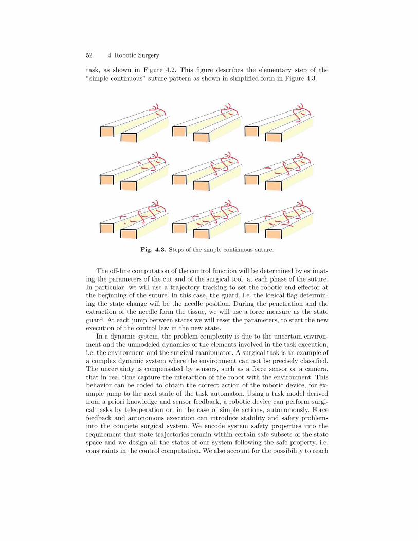
52 4 Robotic Surgery
task, as shown in Figure 4.2. This figure describes the elementary step of the”simple continuous” suture pattern as shown in simplified form in Figure 4.3.
Fig. 4.3. Steps of the simple continuous suture.
The off-line computation of the control function will be determined by estimat-ing the parameters of the cut and of the surgical tool, at each phase of the suture.In particular, we will use a trajectory tracking to set the robotic end effector atthe beginning of the suture. In this case, the guard, i.e. the logical flag determin-ing the state change will be the needle position. During the penetration and theextraction of the needle form the tissue, we will use a force measure as the stateguard. At each jump between states we will reset the parameters, to start the newexecution of the control law in the new state.
In a dynamic system, the problem complexity is due to the uncertain environ-ment and the unmodeled dynamics of the elements involved in the task execution,i.e. the environment and the surgical manipulator. A surgical task is an example ofa complex dynamic system where the environment can not be precisely classified.The uncertainty is compensated by sensors, such as a force sensor or a camera,that in real time capture the interaction of the robot with the environment. Thisbehavior can be coded to obtain the correct action of the robotic device, for ex-ample jump to the next state of the task automaton. Using a task model derivedfrom a priori knowledge and sensor feedback, a robotic device can perform surgi-cal tasks by teleoperation or, in the case of simple actions, autonomously. Forcefeedback and autonomous execution can introduce stability and safety problemsinto the compete surgical system. We encode system safety properties into therequirement that state trajectories remain within certain safe subsets of the statespace and we design all the states of our system following the safe property, i.e.constraints in the control computation. We also account for the possibility to reach
4.5 Conclusion 53
the manual state from each state. We guarantee the continuous evolution (invari-ant set property) and the stability of the complete system by enforcing constraintson the control laws. As an example, we consider the positioning state, the firststate of the suture automaton, and the jump to the following state, i.e. contactwith the tissue. In the first state we use a control law based on the knowledge ofthe exact position and orientation that the needle should have to bite the tissue.The constraints that we take into account are: needle shape, grasp position of themanipulator end effector with respect to the needle, tissue position, and tissueproperties. The jump guard is the force, i.e. when the needle contacts the tissue,a force value is acquired from the force sensor. The state transition constraintsthat we use to preserve stability and safety are: bounded control, this is to ensurebounded output, and requires the knowledge of the tissue viscosity; small devicemovements, so that the kinematic constraints are satisfied during the movementto the contact. In the second state, i.e. tissue perforation, a control law based onthe property of the tissue is used. The manual mode is always reachable when anevent is triggered by the supervisory software or by the surgeon monitoring theoperation. We consider an index weighted on the safety of the task, i.e. how far isthe current execution from the nominal task performance. The higher this indexthe lower the probability that the task will be safely completed.
4.5 Conclusion
In this chapter we have described the state of the art in robotic surgery, withemphasis on teleoperation and segmentation. The classification is used mainly forsafety or training or evaluation issues as described in this Chapter. In the lastSection we describe a suture in terms of a deterministic automaton. We base ouralgorithm on the parameters determined from suture analysis, and we consider thesafety of the execution as a model property.


5
Optimal Control Design
Insofar as the laws of mathematics are certain, they do not refer to reality; and insofaras they refer to reality, they are not certain.
Albert Einstein
In this Chapter we will present the approach we propose to control the au-tonomous execution of a complex task. The task that we consider is a surgicalsuture, using the model developed in Chapter 4. This task, although simple, hasthe characteristics of a complex task, since it require different control modes andinvolves various logical conditions. To guarantee the correct task execution wefirst compute off-line the nominal trajectory of the state variables, using optimiza-tion techniques. At execution time, uncertainties are compensated by a regulator.Roughly speaking, the computation of the nominal trajectory is an instance ofoptimal control problem, i.e. to drive the system to a desirable state while min-imizing a cost function that depends on the path followed. It typically involvesa terminal cost (depending on the terminal state), an integral cost accumulatedalong continuous evolution, and a series of jump cost associated with discrete tran-sitions. This is a classical problem for continuous systems, extended more recentlyto discrete systems [156], and a class of hybrid systems with simple continuousdynamics. The approach has been extended to general hybrid systems using adynamic programming formulation [44], and a variational formulation, extendingPontryagin Maximum Principle [93]. In this Chapter we introduce the optimumsystem control in Section 5.1 and its mathematical background in Section 5.1.2.We explore the optimum control from hybrid system point of view in Section 5.2.In Section 5.3 we present the formulation of the problem addressed in this Thesisand in Section 5.4 we give an explanation of the choices carried out.
5.1 Optimum System Control
The fundamental problem of optimization theory may be subdivided into fourinterrelated parts:
• Definition of a goal.
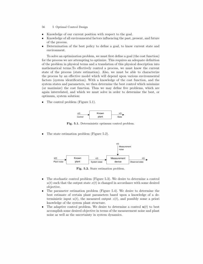
56 5 Optimal Control Design
• Knowledge of our current position with respect to the goal.• Knowledge of all environmental factors influencing the past, present, and future
of the process.• Determination of the best policy to define a goal, to know current state and
environment.
To solve an optimization problem, we must first define a goal (the cost function)for the process we are attempting to optimize. This requires an adequate definitionof the problem in physical terms and a translation of this physical description intomathematical terms.To effectively control a process, we must know the currentstate of the process (state estimation). Also, we must be able to characterizethe process by an effective model which will depend upon various environmentalfactors (system identification). With a knowledge of the cost function, and thesystem states and parameters, we then determine the best control which minimize(or maximize) the cost function. Thus we may define five problems, which areagain interrelated, and which we must solve in order to determine the best, oroptimum, system solution:
• The control problem (Figure 5.1).
Knownplant
u(t)
Control State
x(t)
Fig. 5.1. Deterministic optimum control problem.
• The state estimation problem (Figure 5.2).
Measurementdevice
x(t)
System state Observed state
z(t)Knownplant
w(t)
Plant noise
v(t)Measurementnoise
Fig. 5.2. State estimation problem.
• The stochastic control problem (Figure 5.3). We desire to determine a controlu(t) such that the output state x(t) is changed in accordance with some desiredobjective.
• The parameter estimation problem (Figure 5.4). We desire to determine thebest estimate of certain plant parameters based upon a knowledge of a de-terministic input u(t), the measured output z(t), and possibly some a prioriknowledge of the system plant structure.
• The adaptive control problem. We desire to determine a control u(t) to bestaccomplish some desired objective in terms of the measurement noise and plantnoise as well as the uncertainty in system dynamics.
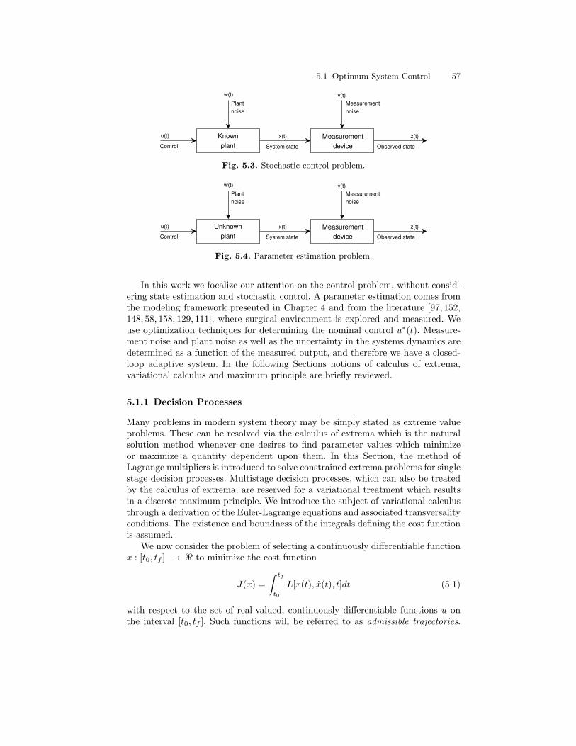
5.1 Optimum System Control 57
Measurementdevice
x(t)
System state Observed state
z(t)Knownplant
u(t)
Control
w(t) v(t)Plantnoise
Measurementnoise
Fig. 5.3. Stochastic control problem.
Measurementdevice
x(t)
System state Observed state
z(t)Unknownplant
u(t)
Control
w(t) v(t)Plantnoise
Measurementnoise
Fig. 5.4. Parameter estimation problem.
In this work we focalize our attention on the control problem, without consid-ering state estimation and stochastic control. A parameter estimation comes fromthe modeling framework presented in Chapter 4 and from the literature [97, 152,148, 58, 158, 129, 111], where surgical environment is explored and measured. Weuse optimization techniques for determining the nominal control u∗(t). Measure-ment noise and plant noise as well as the uncertainty in the systems dynamics aredetermined as a function of the measured output, and therefore we have a closed-loop adaptive system. In the following Sections notions of calculus of extrema,variational calculus and maximum principle are briefly reviewed.
5.1.1 Decision Processes
Many problems in modern system theory may be simply stated as extreme valueproblems. These can be resolved via the calculus of extrema which is the naturalsolution method whenever one desires to find parameter values which minimizeor maximize a quantity dependent upon them. In this Section, the method ofLagrange multipliers is introduced to solve constrained extrema problems for singlestage decision processes. Multistage decision processes, which can also be treatedby the calculus of extrema, are reserved for a variational treatment which resultsin a discrete maximum principle. We introduce the subject of variational calculusthrough a derivation of the Euler-Lagrange equations and associated transversalityconditions. The existence and boundness of the integrals defining the cost functionis assumed.
We now consider the problem of selecting a continuously differentiable functionx : [t0, tf ] → < to minimize the cost function
J(x) =∫ tf
t0
L[x(t), x(t), t]dt (5.1)
with respect to the set of real-valued, continuously differentiable functions u onthe interval [t0, tf ]. Such functions will be referred to as admissible trajectories.
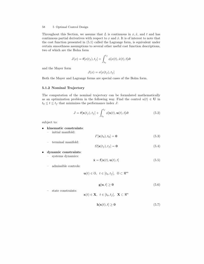
58 5 Optimal Control Design
Throughout this Section, we assume that L is continuous in x, x, and t and hascontinuous partial derivatives with respect to x and x. It is of interest to note thatthe cost function presented in (5.1) called the Lagrange form, is equivalent undercertain smoothness assumptions to several other useful cost function descriptions,two of which are the Bolza form
J(x) = θ[x(tf ), tf ] +∫ tf
t0
φ[x(t), x(t), t]dt
and the Mayer formJ(x) = σ[x(tf ), tf ]
Both the Mayer and Lagrange forms are special cases of the Bolza form.
5.1.2 Nominal Trajectory
The computation of the nominal trajectory can be formulated mathematicallyas an optimization problem in the following way. Find the control u(t) ∈ U int0 ≤ t ≤ tf that minimizes the performance index J :
J = θ[x(tf ), tf ] +∫ tf
t0
φ[x(t),u(t), t]dt (5.2)
subject to:
• kinematic constraints:– initial manifold:
Γ [x(t0), t0] = 0 (5.3)
– terminal manifold:Ω[x(tf ), tf ] = 0 (5.4)
• dynamic constraints:– systems dynamics:
x = f [x(t),u(t), t] (5.5)
– admissible controls:
u(t) ∈ f, t ∈ [t0, tf ], f ⊂ <m
g[u, t] ≥ 0 (5.6)
– state constraints:x(t) ∈ X, t ∈ [t0, tf ], X ⊂ <n
h[x(t), t] ≥ 0 (5.7)
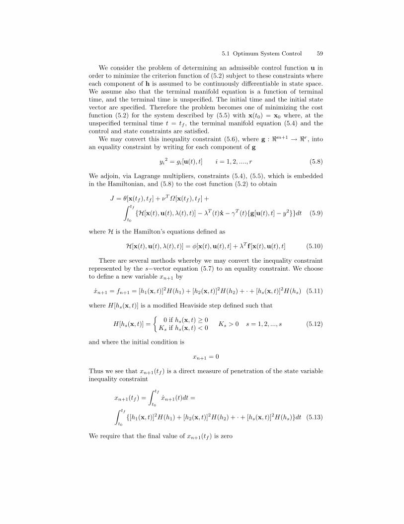
5.1 Optimum System Control 59
We consider the problem of determining an admissible control function u inorder to minimize the criterion function of (5.2) subject to these constraints whereeach component of h is assumed to be continuously differentiable in state space.We assume also that the terminal manifold equation is a function of terminaltime, and the terminal time is unspecified. The initial time and the initial statevector are specified. Therefore the problem becomes one of minimizing the costfunction (5.2) for the system described by (5.5) with x(t0) = x0 where, at theunspecified terminal time t = tf , the terminal manifold equation (5.4) and thecontrol and state constraints are satisfied.
We may convert this inequality constraint (5.6), where g : <m+1 → <r, intoan equality constraint by writing for each component of g
yi2 = gi[u(t), t] i = 1, 2, ...., r (5.8)
We adjoin, via Lagrange multipliers, constraints (5.4), (5.5), which is embeddedin the Hamiltonian, and (5.8) to the cost function (5.2) to obtain
J = θ[x(tf ), tf ] + νTΩ[x(tf ), tf ] +∫ tf
t0
H[x(t),u(t), λ(t), t)]− λT (t)x− γT (t)g[u(t), t]− y2dt (5.9)
where H is the Hamilton’s equations defined as
H[x(t),u(t), λ(t), t)] = φ[x(t),u(t), t] + λT f [x(t),u(t), t] (5.10)
There are several methods whereby we may convert the inequality constraintrepresented by the s−vector equation (5.7) to an equality constraint. We chooseto define a new variable xn+1 by
xn+1 = fn+1 = [h1(x, t)]2H(h1) + [h2(x, t)]2H(h2) + ·+ [hs(x, t)]2H(hs) (5.11)
where H[hs(x, t)] is a modified Heaviside step defined such that
H[hs(x, t)] =
0 if hs(x, t) ≥ 0Ks if hs(x, t) < 0 Ks > 0 s = 1, 2, ..., s (5.12)
and where the initial condition is
xn+1 = 0
Thus we see that xn+1(tf ) is a direct measure of penetration of the state variableinequality constraint
xn+1(tf ) =∫ tf
t0
xn+1(t)dt =∫ tf
t0
[h1(x, t)]2H(h1) + [h2(x, t)]2H(h2) + ·+ [hs(x, t)]2H(hs)dt (5.13)
We require that the final value of xn+1(tf ) is zero
60 5 Optimal Control Design
xn+1(tf ) = 0
which imposes the restriction that the solution does not violate the inequalityconstraint. This approach is a modification by McGill [132] of a similar procedureby Kelley [110] which converts the s-inequality constraints to s equality constraintsof the form
xn+1 = [h1(x, t)]2H(h1) xn+1(t0) = 0xn+2 = [h2(x, t)]2H(h2) xn+2(t0) = 0
......
...xn+s = [hs(x, t)]2H(hs) xn+s(t0) = 0
(5.14)
which are then added to the cost function to obtain
Jmodified = Joriginal +s∑j=1
xn+j(tf ) (5.15)
The multipliers Ks are thus the penalty functions, and Jmodified is minimizedsuch that the constraint region is entered only slightly, if at all. If we requirexn+j(tf ) = 0 for j = 1, 2, ..., s the constraint is, of course, not exceeded at all.
The dynamic optimization presented in this work is based on the necessaryconditions of optimality derived from Pontryagin’s Maximum Principle [122]:
Theorem 5.1. Given a dynamical system governed by the state equations:
dxjdt
= fj(x1, x2, .., xn, u1, u2, .., um)j = 1, 2, .., n
where u ∈ U and U ⊂ Em, independent of x and t, with the performance indexdefined as:
J =∫ tf
t0
L(x(t),u(t))dt
from a given initial manifold Γ at time t0 to a given terminal manifold Ω at timetf , with tf not prescribed, and defining
H(Λ,x,u) = L(x(t),u(t)) + Λ · f(x,u)
where Λ is a vector of Lagrange multiplier functions, then:if u∗(t), t0 ≤ t ≤ tf , is an optimal control, then there exists a nonzero continuousvector function Λ(t) ∈ <n+1, satisfying the co-state equations:
dΛjdt
= −n∑i=0
∂fi(x,u∗(t))∂xj
∣∣∣∣x=x∗(t)
Λi j = 0, 1, . . . , n
with x0 defined by dx0dt = L(x,u), such that:
minu∈UH(Λ(t),x∗(t),u) = H(Λ(t),x∗(t),u∗(t))H(Λ(t),x∗(t),u∗(t)) = 0Λ0(t) = constant ≥ 0
t ∈ [t0, tf ]
Λ1(t), Λ2(t), . . . , Λn(t) is normal to the end manifolds Γ and Ω at t = t0 andt = tf , respectively.
5.1 Optimum System Control 61
We now apply the Euler-Lagrange equations to the cost function (5.15) inorder to obtain the necessary conditions for a minimum, due to McShane [133]and Pontryagin [146], and others. It is thus convenient to define a scalar functionΦ, the Lagrangian for no inequality state constraint, as
Φ[x(t), x(t),u(t), λ(t), γ(t),y(t), t] =H[x(t),u(t), λ(t), t)]− λT (t)x− γT (t)g[u(t), t]− y2 (5.16)
From (5.16) it follows that the Lagrangian for the problem at hand is
Φ = Φ + λn+1[fn+1 − xn+1] (5.17)
We write the Euler-Lagrange equations as
d
dt
∂Φ∂x
− ∂Φ∂x
− ∂fn+1
∂xλn+1 = 0
d
dt
∂Φ∂u
= 0
d
dt
∂Φ∂y
= 0
(5.18)
We call each piecewise continuously differentiable solution of the Euler-Lagrangeequations (5.18) extremal trajectory of the associated variational problem. Thetransversality conditions for this problem are
Ω[x(tf ), tf ] = 0
x(t0) = x0
∂θ
∂tf+∂ΩT
∂tfν +H = 0 fort = tf
∂θ
∂x+∂ΩT
∂xν − λ = 0 fort = tf
xn+1(t0) = xn+1(tf ) = 0 (5.19)
The optimization problem given by equations (5.18) and (5.19) is essentially aMulti Point Boundary Value Problem, since its solution must satisfy the terminalmanifold Ω, the state and co-state constraints. The optimal solution u∗i (t) for the i-subtask is reached when the above necessary conditions of optimality, derived fromPontryagin’s Maximum Principle, are satisfied. We compute the global optimalsolution, i.e. nominal trajectory of the complete task
u∗(t) =n∑i=1
N∑t=0
u∗i (t)
The optimality of the u∗ is assured by null jump cost θi for all i. These conditions(5.19) can be used to check the i optimal solution because we know for each subtaski the terminal configuration manifold Ω.
62 5 Optimal Control Design
In particular, they must be satisfied by the trajectory computed by the nu-merical method. It will be shown in Chapter 6, that a steepest descent algorithmcomputes a solution satisfying the necessary conditions and, therefore, convergesto a target behavior. In Chapter 6 an overview on the computational approach fora Two Point Boundary Value Problem (TPBVP) is presented. The developmentcarried out for the TPVVP can be easily extended to the Multi Point BoundaryValue Problem (MPBVP).
5.2 Hybrid Optimal Control
In the context of Hybrid Systems, the computation of the optimal solution involvesthe selection of a path among the possible states of the hybrid system and thecomputation of the optimal times to jumps from one state to the next.
Controlling the switching times, when possible, and choosing among severalpossible states, whenever such choices are available, gives rise to a rich class ofoptimal control problems. This has motivated efforts to extend classical optimalcontrol principles [44] and to apply dynamic programming techniques [185, 101].While in principle this is possible, the computational complexity of this compu-tation becomes prohibitive: not only does one have to deal with the well-knowncurse of dimensionality in such problems, but there are at least two additionalsources of complexity to deal with, i.e., the presence of switching events causingtransitions from one state to another (which introduces a combinatorial elementinto the control), and the presence of event-driven dynamics for the switchingtimes (which introduce non differentiability). Therefore, key to the successful de-velopment of optimal control methods for hybrid systems is the identification ofstructural properties that allow the decomposition of such systems into simplercomponents, and making use of efficient numerical techniques. Along these lines,progress has been reported for classes of hybrid systems whose structure may beexploited. For example, in [35] a Mixed Logical Dynamical (MDL) system frame-work is proposed, which allows the use of efficient methods developed for piecewiseaffine systems, and in [96] optimal controllers are presented for the class of au-tonomous switched linear systems.
The problem statement defined in Section 5.1.2 must be modified for the case ofHybrid Systems. The Hybrid Optimal Control Problem (HOCP) is to find optimalhybrid (i.e., continuous u and discrete v) control trajectories such that an integralcost index, typically an integral of a function of the hybrid system state and controlinput, is minimized subject to the system dynamics, initial, terminal, and furtherequality or inequality constraints.
The Hybrid Optimal Control Problem is defined as the minimization of thereal valued, hybrid cost index J :
minu,v
J(u,v) = θ[x(t+0 ), . . . ,x(t−N );q(t+0 ), . . . ,q(t−N ); t0, . . . , tN ]+∫ tf
t0
φ[x,u,q,v, t]dt
(5.20)subject to:
• kinematic constraints:
5.2 Hybrid Optimal Control 63
– initial manifold:Γ [x(t0),q(t0)] = 0 (5.21)
– terminal manifold:Ω[x(tf ),q(tf )] = 0 (5.22)
• dynamic constraints:– systems dynamics:
x = f [x,u,q,v, t] if Rj(x,u,q,v, t) 6= 0 j = 1, . . . , ns (5.23)
[x(t+i )q(t+i )
]= Gj(x,u,q,v, t−i ) if Rj(x,u,q,v, t−i ) = 0 j = 1, . . . , ns
(5.24)– admissible controls:
u(t) ∈ f, f ⊂ <nu , v(t) ∈ V, t ∈ [t0, tf ], V ⊂ Znv
g[u,v, t] ≥ 0 t ∈ [t0, tf ] (5.25)
– state constraints:
x(t) ∈ X, X ⊂ <nx , q(t) ∈ Q, t ∈ [t0, tf ], Q ⊂ Znq
h[x,q, t] ≥ 0 t ∈ [t0, tf ] (5.26)
where the initial and final times, t0, tf , are free or fixed, Rj are the ns switchingfunctions and Gj denotes the explicit phase transition conditions occurring at thezeros of the one of the switching functions. θ is a general function of the phasetransition time ti, i = 1, . . . , N and of the continuous x(t−i ), x(t+i ) and discretestates q(t−i ), q(t+i ) just before and just after the N − 1 interior transition eventsand at the beginning and final times respectively. The number of phases N may begiven or free. The integrand ψ is a real-valued function of the continuous/discretestate and control variables and of time.
The solutions of the HOCPs described in the previous equations are deter-ministic open-loop trajectories. As in conventional optimal control this class ofproblems can be generalized to a stochastic setting or to treat issues like opti-mal closed-loop feedback control. The numerical solution of closed-loop hybridfeedback control problems, however, is at even a much earlier stage and the pri-marily finite-element based solution strategies that have been presented for theirsolution [101, 171] cannot readily handle nonlinear systems of more than threedimensions due to the well-known curse of dimensionality. A framework for mod-eling and (optimally) controlling mixed logical dynamical systems described bylinear dynamic equations subject to linear inequalities involving real and integervariables has been proposed by [37]. The on-line optimization problems resultingfrom a predictive control scheme are solved numerically by application of a mixed-integer quadratic programming branch-and-bound method. However, the approachis not applicable to our class of HOCPs with nonlinear dynamics equations sub-ject to nonlinear constraints. For these reasons we adopt Pontryagin’s MaximumPrinciple to the specific requirements of Hybrid Systems
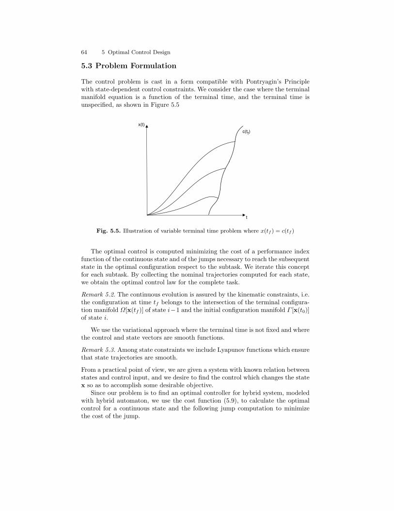
64 5 Optimal Control Design
5.3 Problem Formulation
The control problem is cast in a form compatible with Pontryagin’s Principlewith state-dependent control constraints. We consider the case where the terminalmanifold equation is a function of the terminal time, and the terminal time isunspecified, as shown in Figure 5.5
t
x(t)
c(t )f
Fig. 5.5. Illustration of variable terminal time problem where x(tf ) = c(tf )
The optimal control is computed minimizing the cost of a performance indexfunction of the continuous state and of the jumps necessary to reach the subsequentstate in the optimal configuration respect to the subtask. We iterate this conceptfor each subtask. By collecting the nominal trajectories computed for each state,we obtain the optimal control law for the complete task.
Remark 5.2. The continuous evolution is assured by the kinematic constraints, i.e.the configuration at time tf belongs to the intersection of the terminal configura-tion manifold Ω[x(tf )] of state i−1 and the initial configuration manifold Γ [x(t0)]of state i.
We use the variational approach where the terminal time is not fixed and wherethe control and state vectors are smooth functions.
Remark 5.3. Among state constraints we include Lyapunov functions which ensurethat state trajectories are smooth.
From a practical point of view, we are given a system with known relation betweenstates and control input, and we desire to find the control which changes the statex so as to accomplish some desirable objective.
Since our problem is to find an optimal controller for hybrid system, modeledwith hybrid automaton, we use the cost function (5.9), to calculate the optimalcontrol for a continuous state and the following jump computation to minimizethe cost of the jump.
5.3 Problem Formulation 65
Definition 5.4. We define the cost of the jump as the distance between the initialposition on manifold Γ [x(t0)] of the state i and the final position of terminalmanifold Ω[x(tf )] of the state i − 1. We instantiate the function θ[x(tf ), tf ] assuch distance function.
Remark 5.5. θ is an indicator of successful completion of the task: the bigger θ thelower the probability to complete the task.
We define:
Definition 5.6. Safety in a task execution is the property of completing the taskwithout uncontrolled behaviors.
Thus we can state the following:
Remark 5.7. The distance θ is inversely proportional to the safety of the completesystem execution.
For our problem the function θ[x(tf ), tf ] is the distance between two points onthe same manifold because we assume that:
Remark 5.8. The final configuration manifold Ω[x(tf )] of state i−1 and the initialconfiguration manifold Γ [x(t0)] of state i intersect at tf = t0. The final point ofthe trajectory of the state i− 1 and the initial point of the trajectory of the statei are on this manifold.
To define the concept of the jump cost we introduce the following definitions.
Definition 5.9. A metric is a nonnegative function g(x, y) describing the ”dis-tance” between neighboring points for a given set. A metric satisfies the triangleinequality
g(x, y) + g(y, z) ≥ g(x, z)
and is symmetric, sog(x, x) = 0
andg(x, y) = 0 implies x = y
Definition 5.10. The distance between two points is the length of the path con-necting them. In the plane, the distance between points (x1, y1) and (x2, y2) is givenby the Pythagorean theorem. In general, the distance between points x and y in aEuclidean space <n is given by
d = |x− y| =
√√√√ n∑i=1
|xi − yi|2
Definition 5.11. Suppose for every point x in a manifold M , an inner product〈·, ·〉 is defined on a tangent space TxM of M at x. Then the collection of all theseinner products is called the Riemannian metric.
66 5 Optimal Control Design
For curved or more complicated surfaces, the metric used to compute the distancebetween two points is an integration. With distance we mean the shortest distancebetween two points computed on the surface, i.e. the geodesic. The geodesics in aspace depend on the Riemannian metric, which affects the notions of distance andacceleration, see [77].
Definition 5.12. Let δ(s) be a smooth curve on a manifold M from a to b withδ(0) = a and δ(1) = b. Then δ′(s) ∈ Tδ(s) where Ta is the tangent space of M ata. The curve length of δ with respect to the Riemannian structure is given by∫ 1
0
| δ′(s) |δ(s)ds (5.27)
and the distance d(a, b) between a and b is the shortest distance between a and bgiven by
d(a, b) = infδ:a→b
∫ 1
0
| δ′(s) |δ(s)ds (5.28)
Thus, we can describe the θ function as a geodesic, where M[x(tf )] = 01 isthe manifold representing a subset of the configuration space, considering (5.8).Following (5.28), we can write
θ[x(tf )] = infδ:a→b
∫ 1
0
| δ′(s) |δ(s)ds (5.29)
whereδ =| Γi[x(t0)]−Ωi−1[x(tf )] | with tf = t0 (5.30)
For example for a surface given parametrically by x(u, v), y(u, v), and z(u, v),the geodesic can be found by minimizing the arc length
L =∫ds =
∫ √dx2 + dy2 + dz2
where
dx =∂x
∂udu+
∂x
∂vdv
dx2 = (∂x
∂u)2(du)2 + 2
∂x
∂u
∂x
∂vdudv + (
∂x
∂v)2(dv)2
5.4 Discussion and Conclusions
In summary, the problem addressed in this work can be subdivided in the followingsteps:
• Task modeling, described in Chapter 4.• Formalization as an optimal control problem, presented in Section 5.1.2.
1 M is not explicitly dependent on time as Γ and Ω in this case
5.4 Discussion and Conclusions 67
• Off-line computation of the nominal trajectory satisfying task constraints, de-scribed in Chapter 6.
• On-line simulation of the real system and calculation of the distance functionθ, carried out in this Section.
In this Chapter we focus on the various approaches to optimal trajectory com-putation for different kind of dynamical systems. We define the theoretical frame-work used in this research and motivate the various choices made.
In particular we use a deterministic behavior to describe task evolution (seeChapter 4), i.e. the optimal trajectory accounts for a single switch at each jumpcondition. Hence, we compute the nominal trajectory as explained in Section 5.1.2,by transforming the discrete part of the hybrid system in a set of constraints forthe continuous optimal trajectory computation. This choice of task representationis motivated by the nature of the task we are studying.
With respect to the computation of the optimal solution we do not followthe general HOCP approach making the optimal choice among many switchingpossibilities. Rather, we use a priori knowledge in the switching selection to chooseamong jump alternatives to emphasize good performance in each subtask andsafety of the complete execution. This is accomplished by optimizing a performanceindex based on the the knowledge of the task. We compute the nominal trajectoryimplementing the desired task behavior. In the on-line implementation a weight,a.k.a the distance θ is used as index of good performance. We use PontryaginMaximum Principle because the constraints of the problem at hand can be mappeddirectly into this formulation.
With the approach proposed in this Thesis we want to assure safety, good per-formance and efficiency. In our approach a priory knowledge plays a big role inthe definition of the task model and in the computation of the optimal solution,however this is not a limitation to the solution of more general hybrid controlproblems because of the large number of situations where the optimal execution iswell defined and structured. In fact, it is more appropriate to indicate the approachproposed as the solution to an optimal control problem rather for an hybrid op-timal control problem because we have used the hybrid systems model mostly asmodeling and solution framework. The results of this approach are demonstratedin Chapter 7 with appropriate examples.

6
Computational Issues
You might wish to follow the advice of your authors as notorious computer gunslingers:We always shoot first, and only then relax.
[3]
Theoretical work on controllability properties of nonlinear hybrid dynamicalsystems is still in its early stages and to date only a few problems with low state andcontrol dimensionability can be throughly understood [177]. Nevertheless, therehas been a strong interest in numerical methods for determining controllers forthese systems, inspired from the success of such approaches in conventional non-linear optimal control problems. Nonlinear optimal control plays a key role inmodern mechatronics and robotics, in particular in the area of path, trajectory,and action planning. To mention some of the many applications: walking patternand trajectory planning [98], mobile robot path planning [113], optimal payload(weight) lifting, and acrobatics [8, 130], etc.. Numerical algorithms designed forhybrid optimal control problems (HOCPs) with variable structure and nonlineardifferential equations have recently been published [55,101,171]. The key to numer-ically solving HOCPs seems to be the combination of efficient numerical solvers,such as direct collocation, for optimal control problems together with (heuristic)approaches to reduce the combinatorial complexity of the discrete event aspect inHOCPs [55,180].
The organization of this Chapter is as follows: in Section 6.1 a broad classof HOCPs is defined and numerical strategies to obtain suboptimal solutions oninterior point constraints on grids are summarized, Section 6.1.1, and a branch-and-bound strategy, Section 6.1.2, is proposed. The approach of this work is pre-sented in Section 6.2 and in particular in Section 6.3 the algorithm implementedis discussed, that relies on an efficient numerical tool developed in Matlab [53].
6.1 HOCP Solutions
A set of several different numerical strategies is presented here to compute the solu-tion to the HOCP. Two alternatives HOCP solution strategies will be described: (i)
70 6 Computational Issues
suboptimal solution with interior event time and state constraints fixed on a gridcombined with graph search, and (ii) transformation to a mixed-binary-optimalcontrol problem and its subsequent solution using a branch-and-bound algorithm.
6.1.1 Suboptimal Solution Technique
Suboptimal solutions may be obtained by assigning interior point time instantsand states to predefined values on a (fine) grid. Between grid points, a standardoptimal control problem with fixed boundary conditions is solved. Finally, thesuboptimal solution to the HOCP is obtained by a graph search with each gridpoint forming the nodes of the graph and the optimal cost weighing the vertices ofthe graph. This solution strategy is applied to solve cooperative multi-arm trans-port problem [55]. Disadvantages of this approach are the possibly high number ofmulti-point boundary value problems to be solved and the inherent suboptimalityof the solution obtained. On the other hand, an appealing advantage is that byproblem understanding one often has good insight as to how the grid needs to bespecified, and a useful solution usually can be obtained easily.
Sparse Direct Collocation
The basis for the suboptimal solution strategies is the highly efficient direct collo-cation method implemented in the software package Dircol [179] to approximatelysolve optimal control problems using solutions to (sparse) nonlinear programming.
The numerical method of sparse direct collocation implemented in Dircol canefficiently solve multi-phase optimal control problems with a fixed discrete statetrajectory. The state x is approximated by cubic Hermite polynomials x =
∑j αj x
and the control vector u by piecewise linear functions u =∑k αkx on a discretized
grid in each phase. The state differential equations are pointwise fulfilled at thegrid points and grid midpoints, resulting in a set of nonlinear program (NLP)equality constraints. The control or state inequality constraints are to be satis-fied at the grid points resulting in a set of nonlinear NLP inequality constraints.The transcription of the optimal control problem to an NLP is made by Dircol, theNLP is solved efficiently with the advanced SQP-based (Sequential Quadratic Pro-gramming) sparse nonlinear program solver SNOPT [91], and subsequently Dircolprocesses the solution to provide state and control trajectories, error estimatesand output that may be used to verify the optimality of the solution. Importantfeatures of the method are:
• As the grid becomes finer, the discretized solution converges to a solution of theEuler-Lagrange differential equations (EL-DEQs) according to the MaximumPrinciple.
• Reliable estimates of the adjoint variable trajectories λ along the discretizationgrid may be derived from the Lagrange multipliers of the NLP. They enablea verification of the optimality conditions of the discretized solution withoutsolving explicitly the EL-DEQs.
• Local optimality error estimates can be derived which enable efficient strategiesfor successively refining a first solution on a coarse grid.
6.2 TPBVP Solutions 71
• Computation is fast because ODE simulation and control optimization areperformed simultaneously (unlike shooting methods).
• The method is also applicable to systems described by differential-algebraicequations of differential index 1. In this case, the algebraic state variables arediscretized analogously to the control variables by piecewise linear functions.
6.1.2 Branch-and-Bound
The solution method for mixed-binary optimal control problems (MBOCP) using acombination of sparse direct collocation and branch-and-bound was first presentedin [178] and further investigated in [180,55]. Given certain assumptions (finite andknown number of phases, constant state and control variables), the HOCP may betransformed into a MBOCP with a simple transformation of its discrete variables.
The solution of the MBOCP yields the optimal (open loop) trajectories, theoptimal phase transition times, the possibly free final time and the optimal binarycontrol vector.
Remark 6.1. The nature of the binary control vector appearing in the MBOCP istwofold. On the one hand it represents the discrete control variable v that controlsthe order and types of phase transitions, on the other hand it also represents thediscrete state q in each phase.
A branch-and-bound strategy in combination with a binary search tree is em-ployed. The subproblems solved provide approximate upper and lower bounds tothe MBOCP performance index. If the lower bound at a node is greater thanthe global upper bound, that branch is discarded. The comparison of subproblemsolutions is additionally aided by the use of the optimality error estimate (confi-dence interval). The MBOCP is thus reduced to a continuous multi-phase optimalcontrol problem, that is a relaxation method (see definition in the following).
6.2 TPBVP Solutions
Unless system equations, performance index, and constraints are quite simple, wemust employ numerical methods to solve optimal programming and control prob-lems. Optimal programming and control problems are at least two point boundaryvalue problems (TPBVP) and, in some cases, multi point boundary value prob-lems (MPBVP), e.g. when there are interior point constraints or state variableinequality constraints.
Finding solutions to these nonlinear two-point boundary-value problem is, inmany cases, not a trivial extension of finding solutions to initial-value (one-pointboundary-value) problems. The crucial distinction between initial value problemsand TPBVP is that in the former case we are able to start an acceptable solutionat its beginning (initial values) and just march along it by numerical integrationto its end (final values). In the present case, instead the boundary conditions atthe starting point do not determine a unique solution to start with, and a randomchoice among the solutions which satisfy these (incomplete) starting boundaryconditions is almost certain not to satisfy the boundary conditions at the other
72 6 Computational Issues
specified points. Iteration is generally required to mold these spatially scatteredboundary conditions into a single global solution of the differential equations. Forthis reason, TPBVP require considerably more effort to solve than do initial valueproblems.
The nonlinear two-point boundary value problem can be defined as
Definition 6.2. Find the n state variables, x(t), the n influence functions, λ(t)and the m control variables, u(t) to satisfy, simultaneously, the n system differen-tial equations (involving x, u), the n influence (adjoint, Euler-Lagrange) differen-tial equations (involving λ, x, u), the m optimality conditions (involving λ, x, u)and the initial and final boundary conditions (involving λ, x)
There are two distinct classes of numerical methods for solving TPBVPs. In theshooting (or direct) method we choose values for all of the dependent variables atone boundary. These values must be consistent with any boundary conditions forthat boundary, but otherwise are arranged to depend on arbitrary free parameterswhose values we initially ’randomly’ guess. We then integrate the ODEs by initialvalue methods, arriving to the other boundary (and/or interior points with bound-ary conditions specified). The shooting method provides a systematic approach totaking a set of ’ranging’ shots that allow us to improve our aim systematically.In all shooting methods, trial solutions satisfy the differential equations ’exactly’,but the trial solutions come to satisfy the required boundary conditions only afterthe iterations are finished.
In the relaxation (or indirect) methods differential equations are replaced byfinite difference equations on a mesh of points that cover the range of the inte-gration. The iteration, called relaxation, consists of adjusting all the values on themesh so as to bring them into successively closer agreement with the finite dif-ference equations and, simultaneously, with the boundary conditions. Good initialguesses are the secret of efficient relaxation methods.
Relaxation works best when the solution is smooth and not highly oscillatory,such oscillations would require many grid points for accurate representation. Thenumber and position of required points may not be known a priori. Shooting meth-ods are usually preferred in such cases, because their variable step-size integrationsadjust naturally to a solution’s peculiarities.
6.2.1 The Calculus of Variation and Optimal Control
The extrema-finding techniques, although quite sufficient for many different situ-ations, will not, in general, yield the solution to many problems associated withcontrol systems. Whereas the previously discussed techniques deal with methodsfor extremizing functions of one or several independent variables, in control sys-tem design we are typically concerned with extremizing certain types of functionswhose independent variables are actually other functions. This type of function iscalled a functional. Although, as we might expect, many of the basic approaches forextremizing functionals are similar to those for extremizing functions, the resultsare sometimes quite different. The body of mathematics developed for extremiz-ing functionals is variational calculus. Variational principles have been applied tophysical problems, such as wave propagation. The Hamiltonian formulation of the

6.2 TPBVP Solutions 73
variational problem has existed since the early nineteenth century in the works ofHamilton, Jacobi, and others. The most significant contribution in recent timeswas made by L.S. Pontryagin. The work of Pontryagin [146] extended the varia-tional method to include problems wherein the available control and state vectoris bounded, as we have seen in Chapter 5.
We formalize the optimum control problem as MPBVP using variational calcu-lus. This set of differential equation may not be solved in a straightforward mannerbecause of the occurrence of state conditions together with terminal conditions.We use direct methods to change the variational problem into a problem of or-dinary maxima and minima. The techniques commonly used for this purpose arethe Rayleigh-Ritz and the finite elements methods (FEM) [66, 109, 90]; discretedynamic programming [79,32,33] and gradient method or method of steepest de-scend [110,53].
The Ritz and FEM methods [66, 109, 90] are based on finding a sequence offunctions which give successively smaller values to the functional to be minimized.In the Ritz method, for example, the trajectory and the control are expanded interms of a weighted sum of a suitable set of functions, and a minimizing set ofcoefficients for these functions is found. These methods apparently have not beentoo popular due to the difficulties in finding a suitable set of basis functions andin determining the number of terms to use in the expansion.
Another direct method is that of discrete dynamic programming [79,31,32,33].Discrete dynamic programming is, in effect, the repeated, sequential, stage-by-stage application of the Hamilton-Jacobi equations or the optimality principleof Bellman. Discrete dynamic programming has an advantage of actually beingsimplified by the addition of control and state-space constraints. Its biggest dis-advantage is the requirement for a truly fantastic amount of computer memoryfor any but very low order problems. The polynomial approximation method ofBellman [33] and the state increment method of Larson [118] are two methodsfor the reduction of the memory requirements in the computational solution ofoptimal control problems by discrete dynamic programming.
A third and significantly different type of direct method is the gradient methodor method of steepest descent. The gradient method consists of searching for anoptimum by making each new iteration move in the direction of the gradient whichpoints locally in the direction of the maximum decrease (or increase) of the costfunction. The method was developed and applied to optimal control problemsby Kelly [110], and Bryson and Denham [52]. Various modifications to includepenalty functions and other methods of treating equality and inequality constraintshave been presented [53]. We use the approach of Bryson [53]. These gradientmethods have the ability to generate successively improved trajectory with verypoor starting values. However they tend to converge slowly and often require theselection and adjustment of several convergence parameter. The gradient methodis a first-order method since it is based on finding first-order effects of controlupon terminal constraints and the cost function. To improve the convergence ofthe gradient method near the optimal trajectory, second-order term can be added.Due to the similarity of these terms to the terms present in the second variation,these methods are know as methods based on second variations [135, 53]. They
74 6 Computational Issues
do accelerate convergence of the gradient method but they require good initialestimates of the initial control and trajectory for convergence.
The method of quasilinearization for the resolution of boundary-value problemsarising in the solution of nonlinear differential equation has been widely developedand applied by Bellman and Kalaba in various works [34]. This method generatesa monotone iteration scheme whose iterates converge quadratically to a uniquesolution of the problem at hand. This overview does not aim at reviewing the entireliterature of the two-point boundary value problem. A more complete summaryyou can find in [154].
To compute the nominal control function, we use a modified gradient methodbecause we do not fix a target function, a.k.a. the control law, and we do notcompute with the gradient method only a set of parameters but also a controlfunction u(t) that respects the behavioral constraints imposed by the subtaskanalysis. In Chapter 7 we present an application of this methods to the simulationof a robot task touching and breaking a compliant surface. In Section 6.3 wedescribe the algorithm that we use in this work for the generation of the subtasknominal trajectory.
6.3 The Algorithm
We describe in this Section the procedure used to resolve the multi-point boundary-value problem. We transform the variational problem into a minimization problemwith constraints. We minimize a functional and the output of the minimization isthe control law.
The mathematical background for this kind of problem is well defined butvery few implementation results are present in the literature for such kind ofminimization, where we do not have an objective function to minimize, neither weare checking for optimal parameters of this function but we compute a functional.We adapt Brayson’s algorithm [53] to our problem formulation. The algorithmgives the possibility to choose between a fixed time with interval 0 < t < T andopen final time, where t is variable. In the second case the optimization algorithmreturns an optimal control law, with 0 < t < T where T is determined from theproblem constrains. We resolve a dynamic optimization problem with open finaltime, with state and control constraints. The inequality in the state and controlconstrains are added to the problem as shown in Equations (6.1), (6.2) and (6.3).Consider an optimization problem with only one control variable u(t), where u isbounded between umin and umax. We first introduce a change of control variablesfrom u to u1 where
u =(umax + umin)
2+ u1
(umax − umin)2
(6.1)
Using the new control variable u1, we have
−1 ≤ u1 ≤ 1 (6.2)
To handle this constraint, we next introduce a slack control variable u2 where

6.3 The Algorithm 75
u1 = cos (u2) (6.3)
Numerical solutions using u2 as control are then relatively straightforward usingthe gradient projection algorithm seqopt. However, if the exact solution containsabrupt switches from u1 = 1 to u1 = −1 or vice-versa, the solution using u2 willhave rapid but not abrupt changes, so it is an approximate solution. By increasingthe number of integration steps, one can come as close as desired to the exactsolution. If the inequality constraint involves only the state variables, we have tointroduce one or more slack state variables as well as a slack control variable.
Necessary Condition for a Stationary Solution
We state the problem as to find the control vector sequence u(i), i = 0, . . . , N − 1and the time step ∆ to minimize
J = φ[x(N),∆] (6.4)
where the number of steps N is specified and
N∆ = tf (6.5)
subject to the constraints
x(i+ 1) = f [x(i), u(i),∆], x(0) = x0 (6.6)ψ[x(N),∆] = 0 (6.7)
The new element depends on the performance index, terminal constraints, anddynamic equations on the time step ∆. Differential changes in the performanceindex and the terminal constraints are given by
dφ = φ∆d∆+N−1∑i=0
[Huφ(i)du(i) +H∆
φ(i)d∆] (6.8)
dψ = ψ∆d∆+N−1∑i=0
[Huψ(i)du(i) +H∆
ψ(i)d∆] (6.9)
where Hu and H∆ are computed by backward sequencing the adjoint equation forthe performance index
(Huφ(i))T = fu
Tλφ(i+ 1), λφ(N) = φxT (6.10)
H∆φ(i) = f∆
Tλφ(i+ 1) (6.11)λφ(i) = fx
Tλφ(i+ 1) (6.12)
and the adjoint equations for the terminal constraints
(Huψ(i))T = fu
Tλψ(i+ 1), λψ(N) = ψxT (6.13)
H∆ψ(i) = f∆
Tλψ(i+ 1) (6.14)λψ(i) = fx
Tλψ(i+ 1) (6.15)
76 6 Computational Issues
Note that ψ and hence Huψ and H∆
ψ are q-vectors, and λψ is an n × q matrix.To simplify the notation, we define
φ∆4= φ∆ +
N−1∑i=0
H∆φ(i) (6.16)
ψ∆4= ψ∆ +
N−1∑i=0
H∆ψ(i) (6.17)
We adjoin the terminal constraint changes to the performance index changes withconstant Lagrange multipliers ν
dΦ = dφ+ νT dψ
= (φ∆ + νT ψ∆)d∆+N−1∑i=0
[Huφ(i) + νTHu
ψ(i)]du(i) (6.18)
For dΦ = 0 for arbitrary d∆ and du(i), with dψ = 0, it is necessary that
Φ∆4= φ∆ + νT ψ∆ = 0 (6.19)
and thatHu(i)
4= Hu
φ(i) + νTHuψ(i) = 0 (6.20)
for i = 0, . . . , N − 1, where ν is chosen to satisfy ψ = 0.
Remark 6.3. 6.20 is the same condition also with fixed final time.
Remark 6.4. 6.19 is the transversality condition. It is the additional condition thatdetermines the optimal time step ∆.
Numerical Solution with Gradient Methods
Using a guess for the optimal u(i) and optimal ∆, we may calculate the gradientsin (6.19) and (6.20). In general, they will not be zero, so we construct improvedestimates by making differential changes in the negative direction of these gradi-ents:
d∆ = −k∆Φ∆ (6.21)du(i) = −kuHu(i), i = 0, . . . , N − 1 (6.22)
Substituting (6.21)-(6.22) into (6.18) gives
dΦ = −k∆(Φ∆)2 − ku
N−1∑i=0
[Hu(i)HuT (6.23)
which is non-positive if k∆ and ku are chosen positive.Substituting (6.21)-(6.22) into (6.9) gives q linear equations for the q-vector ν:
6.4 Conclusions 77
ν = −(k∆ψ∆ψT∆ + kuQ)−1
(dψ + k∆φ∆ψ∆ + kug) (6.24)
and
Q =N−1∑i=0
[Huψ(i)[Hu
ψ(i)]T
(6.25)
g =N−1∑i=0
[Huφ(i)[Hu
ψ(i)]T
(6.26)
Remark 6.5. (k∆ψ∆ψT∆ + kuQ) is non-singular.
A Matlab code for Problems with Open final Time
A Matlab code for solving open final time problems, called seqopt, is an iterativealgorithm and it follows these summarized steps:
• Compute an initial ∆, tf is divided by N , the number of elements of the controlvector, that is the function to be minimized.
• Initialize states of the systems.• Compute the entire state sequence.• Compute the partial derivative for the dynamics, the objective function and
the constraints respect to the states the control and the time.• Compute the new control in the gradient direction given in the previous step.
Also a new tf is given.• Iteratively perform the algorithm from the initialization step till a maximum
number of steps (fixed) or the difference between the solution of one steps andthe following is less than a threshold.
6.4 Conclusions
In this chapter an overview on numerical algorithms to resolve the optimal controlproblem is given. Some specific methods are proposed in the literature to resolvethe Hybrid Optimal Control Problem. The focus of this algorithms is on the dis-crete evolution, with a search along the graph of the discrete states they computean optimal time trajectory. Instead, we focus on the continuous part and we mini-mize dynamic parameters strictly correlated to the optimal task execution criteria.We constrain the continuous trajectory in each subtask in order to minimize thecost and have a null jump cost. The discrete part is considered only at the final stepwhere the partial results coming from the computation of the nominal trajectoryare putted together to obtain the optimal trajectory for the hybrid system.

7
Computation Results and Simulations
‘Testing can show the presence of bugs, but not their absence.Edsger W. Dijkstra
The simulation of technical processes by scientific computing has become animportant tool for the development of new technologies. In many applications,the required theoretical validation and experimental research can be replaced inpart by numerical computations. In this Chapter, we focus on the simulation ofthe hybrid system optimization described in the previous Chapter and on thepresentation and discussion of the computation results.
7.1 Introduction
Several recently developed efficient numerical methods have been presented inChapter 6. Their impact in engineering is demonstrated by their application tothree different classes of problems, namely trajectory optimization, parameter es-timation and design optimization.
The application of numerical optimization methods to trajectory optimizationfor industrial robots has shown that large improvements are possible comparedwith traditional path planning methods (e.g. [181]). But the use of sophisticatednumerical optimization methods requires several necessities as, e.g., the properdescription of the dynamic behavior of the robot as an n-body system (in minimalcoordinates, e.g., the relative angles between successive joints q = (q1, . . . , qn)T ofthe robot)
M(q(t)q(t) = u(t) + χ(q(t), q(t)), t ∈ [0, tf ] (7.1)
where u = (u1(t), · · · , un(t))T is the torque control, M is the positive definiteand symmetric (n × n)-matrix of moments of inertia and χ are the momentsresulting from centrifugal, coriolis, gravitational and frictional forces. Thus thefirst basic problem is the modeling of the dynamic system (7.1) of the robot.The identification of unknown dynamic parameters of the specific robot (as, e.g.,moments of inertia or friction parameters) is a second must, see Chapter 8.

80 7 Computation Results and Simulations
Once the dynamic equations have been modeled and determined in a properway, the optimization of trajectories can be investigated. Different robot tasks re-quire different objectives for optimal trajectories evolution, e.g., in welding optimaltracking of the prescribed path might be required. For example if only the initialand the final position of the robot are prescribed a fast point-to-point movementmight be requested.
Remark 7.1. The fastest point-to-point motion is calculated with this objectivefunction: tf → min
Remark 7.2. Time minimization in a robotics task exhibits quite often a surpris-ingly result, impacts enormous stress on manipulator links and can even often notbe realized in practice.
Remark 7.3. Fast minimum energy motions has∫ tf0
∑ni=1 ui
2(t)dt → min as ob-jective function.
Remark 7.4. Energy minimization in a robotics task offers a compromise betweentime and stress, [181].
The robot trajectories execution also have to satisfy several constraints as,e.,g., constraints on the controls, the angles and the angular velocities (dynamicalconstraints). Further constraints result from the geometrical design of the robot’sworkspace and require an efficient modeling of collision avoidance (kinematic con-straints).
In this Chapter the concepts presented in this Thesis are explained. In Sec-tion 7.2 computation results of the algorithm explained in the Section 6.3 for a1-DOF manipulator puncturing a membrane are proposed. In Section 7.3 we usethese results, i.e. the nominal control law, as a reference in the closed-loop sys-tem simulation, where a feedback control law is introduced to compensate thedisturbances of the model use for the nominal trajectory computation.
7.2 Nominal Trajectory Computation
In this Section we study a simple robotic switching task, whose hybrid model isshown in Figure 7.1. This diagram represent a simplified surgical action, i.e. theinitial steps of a suture as describes in Section 4.4. The first state represents thesubtask of positioning the end effector of the manipulator in contact with a com-pliant surface; in the second state an elastic force is opposing the tool tip untilthe force applied by robot breaks the surface. At the breaking point there is atransition to the third state in which the end effector of the manipulator movesthrough the surface and stop as soon as possible. For the sake of simplicity, weconsider a 1-DOF manipulator in order to have simple dynamics and simplifiedconstraints. Given the cost function (5.2) and the dynamic and kinematic con-straint, we instantiate them for each state in the automaton (Figure 7.1). In thefirst positioning state we want to minimize the dissipated energy, i.e. φ[u(t)] = u2
while satisfying the dynamic of our system, i.e. for the 1DOF manipulator:
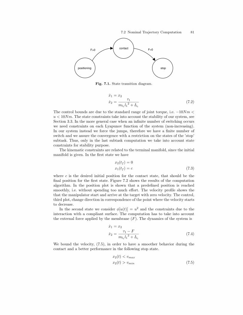
7.2 Nominal Trajectory Computation 81
contact
stoppositioning
F=0F>0
Fig. 7.1. State transition diagram.
x1 = x2
x2 =τ1
ml1 l12 + Il1
(7.2)
The control bounds are due to the standard range of joint torque, i.e. −10Nm <u < 10Nm. The state constraints take into account the stability of our system, seeSection 3.3. In the more general case when an infinite number of switching occurswe need constraints on each Lyapunov function of the system (non-increasing).In our system instead we force the jumps, therefore we have a finite number ofswitch and we assure the convergence with a restriction on the states of the ’stop’subtask. Thus, only in the last subtask computation we take into account stateconstraints for stability purpose.
The kinematic constraints are related to the terminal manifold, since the initialmanifold is given. In the first state we have
x2(tf ) = 0x1(tf ) = c (7.3)
where c is the desired initial position for the contact state, that should be thefinal position for the first state. Figure 7.2 shows the results of the computationalgorithm. In the position plot is shown that a predefined position is reachedsmoothly, i.e. without spending too much effort. The velocity profile shows thethat the manipulator start and arrive at the target with zero velocity. The control,third plot, change direction in correspondence of the point where the velocity startsto decrease.
In the second state we consider φ[u(t)] = u2 and the constraints due to theinteraction with a compliant surface. The computation has to take into accountthe external force applied by the membrane (F ). The dynamics of the system is
x1 = x2
x2 =τ1 − F
ml1 l12 + Il1
(7.4)
We bound the velocity, (7.5), in order to have a smoother behavior during thecontact and a better performance in the following stop state.
x2(t) < vmax
x2(t) > vmin (7.5)
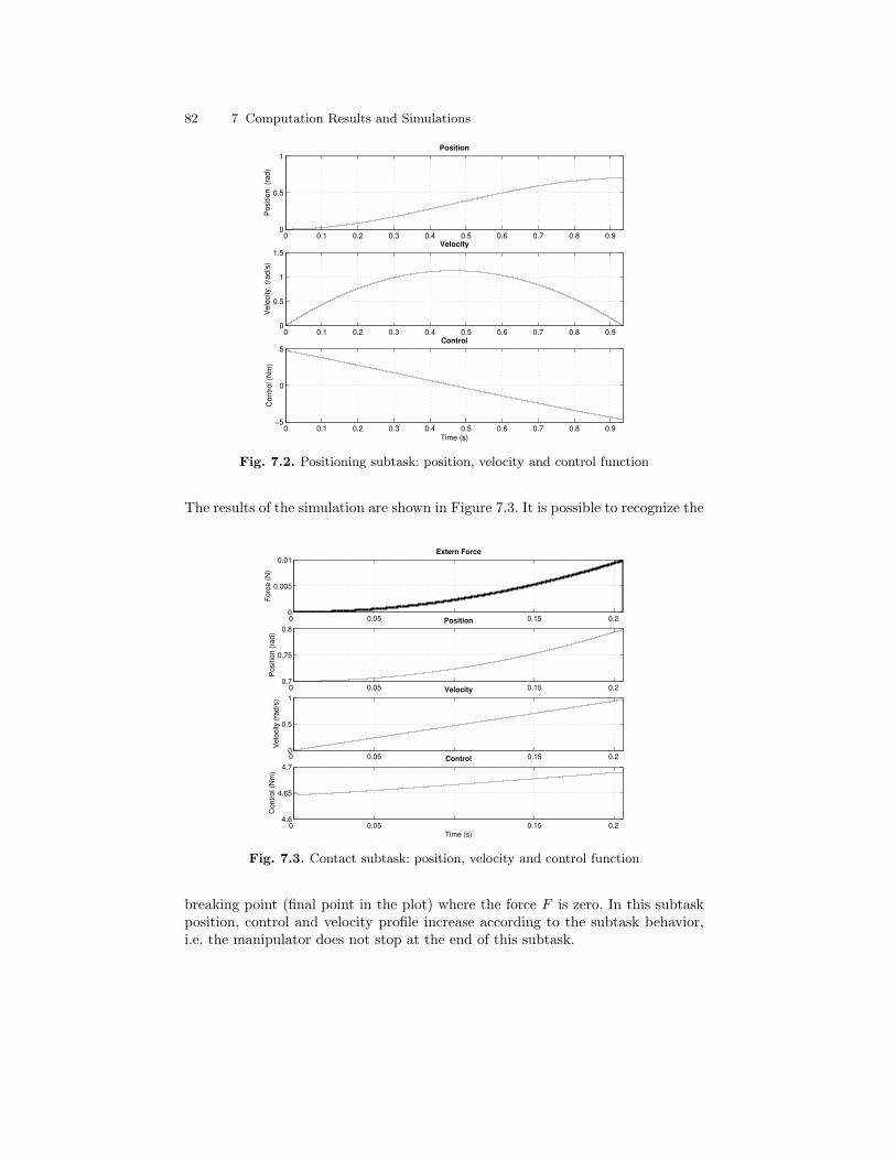
82 7 Computation Results and Simulations
0 0.1 0.2 0.3 0.4 0.5 0.6 0.7 0.8 0.90
0.5
1Position
Pos
ition
. (ra
d)
0 0.1 0.2 0.3 0.4 0.5 0.6 0.7 0.8 0.90
0.5
1
1.5Velocity
Vel
ocity
. (ra
d/s)
0 0.1 0.2 0.3 0.4 0.5 0.6 0.7 0.8 0.9−5
0
5Control
Time (s)
Con
trol (
Nm
)
Fig. 7.2. Positioning subtask: position, velocity and control function
The results of the simulation are shown in Figure 7.3. It is possible to recognize the
0 0.05 0.15 0.2 0
0.005
0.01Extern Force
Forc
e (N
)
0 0.05 0.15 0.2 0.7
0.75
0.8Position
Pos
ition
(rad
)
0 0.05 0.15 0.2 0
0.5
1Velocity
Vel
ocity
(rad
/s)
0 0.05 0.15 0.2 4.6
4.65
4.7Control
Time (s)
Con
trol (
Nm
)
Fig. 7.3. Contact subtask: position, velocity and control function
breaking point (final point in the plot) where the force F is zero. In this subtaskposition, control and velocity profile increase according to the subtask behavior,i.e. the manipulator does not stop at the end of this subtask.
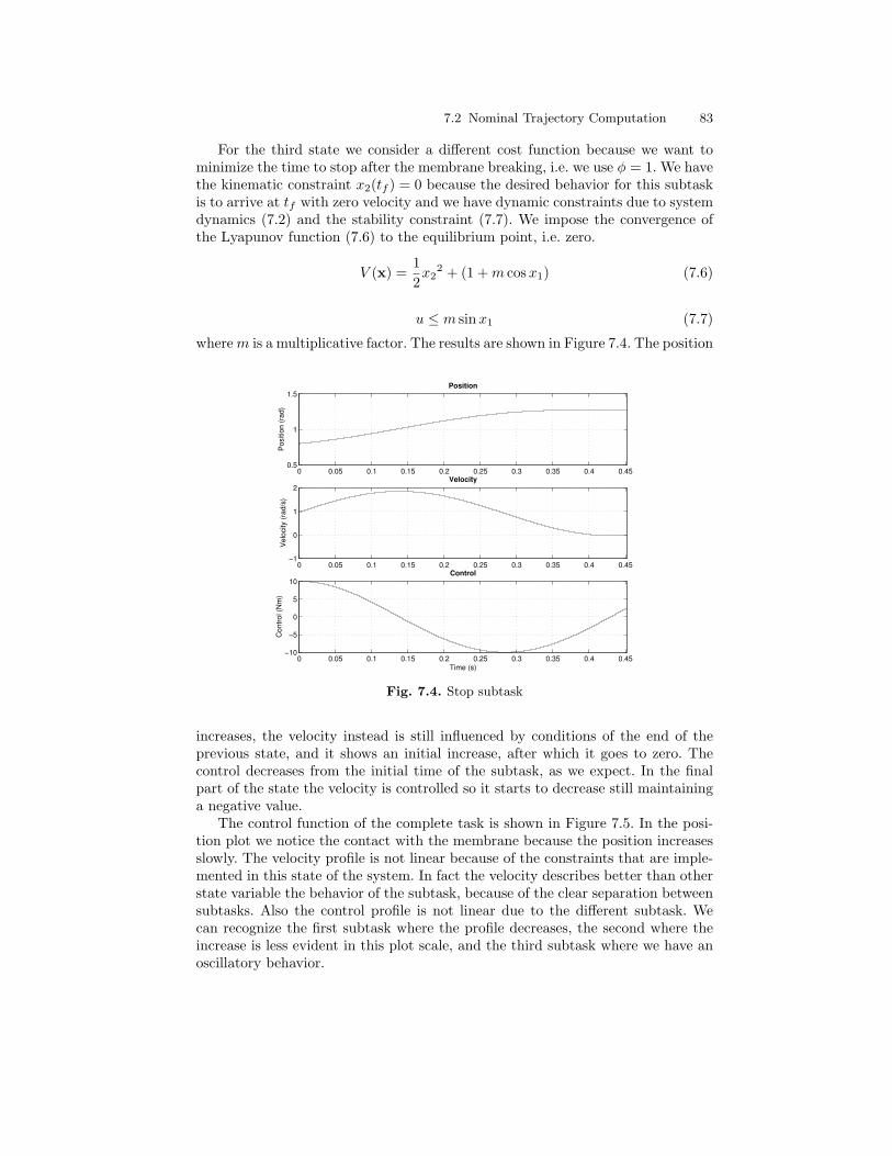
7.2 Nominal Trajectory Computation 83
For the third state we consider a different cost function because we want tominimize the time to stop after the membrane breaking, i.e. we use φ = 1. We havethe kinematic constraint x2(tf ) = 0 because the desired behavior for this subtaskis to arrive at tf with zero velocity and we have dynamic constraints due to systemdynamics (7.2) and the stability constraint (7.7). We impose the convergence ofthe Lyapunov function (7.6) to the equilibrium point, i.e. zero.
V (x) =12x2
2 + (1 +m cosx1) (7.6)
u ≤ m sinx1 (7.7)
wherem is a multiplicative factor. The results are shown in Figure 7.4. The position
0 0.05 0.1 0.15 0.2 0.25 0.3 0.35 0.4 0.450.5
1
1.5Position
Pos
ition
(rad
)
0 0.05 0.1 0.15 0.2 0.25 0.3 0.35 0.4 0.45−1
0
1
2Velocity
Vel
ocity
(rad
/s)
0 0.05 0.1 0.15 0.2 0.25 0.3 0.35 0.4 0.45−10
−5
0
5
10Control
Time (s)
Con
trol (
Nm
)
Fig. 7.4. Stop subtask
increases, the velocity instead is still influenced by conditions of the end of theprevious state, and it shows an initial increase, after which it goes to zero. Thecontrol decreases from the initial time of the subtask, as we expect. In the finalpart of the state the velocity is controlled so it starts to decrease still maintaininga negative value.
The control function of the complete task is shown in Figure 7.5. In the posi-tion plot we notice the contact with the membrane because the position increasesslowly. The velocity profile is not linear because of the constraints that are imple-mented in this state of the system. In fact the velocity describes better than otherstate variable the behavior of the subtask, because of the clear separation betweensubtasks. Also the control profile is not linear due to the different subtask. Wecan recognize the first subtask where the profile decreases, the second where theincrease is less evident in this plot scale, and the third subtask where we have anoscillatory behavior.
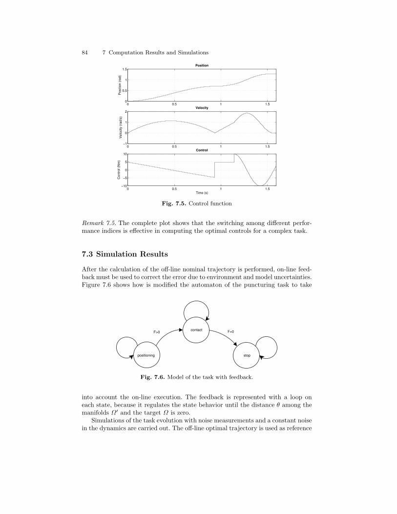
84 7 Computation Results and Simulations
0 0.5 1 1.50
0.5
1
1.5Position
Pos
ition
(rad
)
0 0.5 1 1.5−1
0
1
2Velocity
Vel
ocity
(rad
/s)
0 0.5 1 1.5−10
−5
0
5
10Control
Time (s)
Con
trol (
Nm
)
Fig. 7.5. Control function
Remark 7.5. The complete plot shows that the switching among different perfor-mance indices is effective in computing the optimal controls for a complex task.
7.3 Simulation Results
After the calculation of the off-line nominal trajectory is performed, on-line feed-back must be used to correct the error due to environment and model uncertainties.Figure 7.6 shows how is modified the automaton of the puncturing task to take
contact
stoppositioning
F=0F>0
Fig. 7.6. Model of the task with feedback.
into account the on-line execution. The feedback is represented with a loop oneach state, because it regulates the state behavior until the distance θ among themanifolds Ω′ and the target Ω is zero.
Simulations of the task evolution with noise measurements and a constant noisein the dynamics are carried out. The off-line optimal trajectory is used as reference
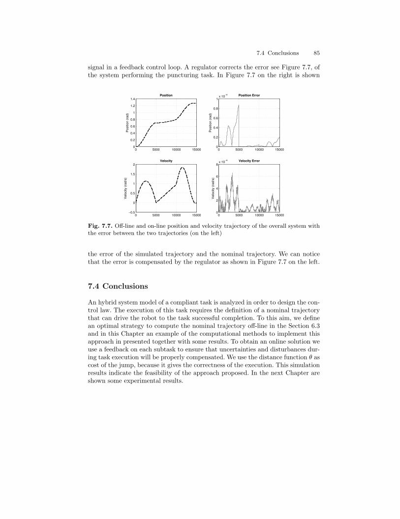
7.4 Conclusions 85
signal in a feedback control loop. A regulator corrects the error see Figure 7.7, ofthe system performing the puncturing task. In Figure 7.7 on the right is shown
0 5000 10000 150000
0.2
0.4
0.6
0.8
1
1.2
1.4Position
Pos
ition
(rad
)
0 5000 10000 15000−0.5
0
0.5
1
1.5
2Velocity
Vel
ocity
(rad
/s)
0 5000 10000 150000
0.2
0.4
0.6
0.8
1x 10⁻⁴ Position Error
Pos
ition
(rad
)0 5000 10000 15000
0
2
4
6
8x 10⁻⁴ Velocity Error
Vel
ocity
(rad
/s)
Fig. 7.7. Off-line and on-line position and velocity trajectory of the overall system withthe error between the two trajectories (on the left)
the error of the simulated trajectory and the nominal trajectory. We can noticethat the error is compensated by the regulator as shown in Figure 7.7 on the left.
7.4 Conclusions
An hybrid system model of a compliant task is analyzed in order to design the con-trol law. The execution of this task requires the definition of a nominal trajectorythat can drive the robot to the task successful completion. To this aim, we definean optimal strategy to compute the nominal trajectory off-line in the Section 6.3and in this Chapter an example of the computational methods to implement thisapproach in presented together with some results. To obtain an online solution weuse a feedback on each subtask to ensure that uncertainties and disturbances dur-ing task execution will be properly compensated. We use the distance function θ ascost of the jump, because it gives the correctness of the execution. This simulationresults indicate the feasibility of the approach proposed. In the next Chapter areshown some experimental results.

8
Experimental Verification
Hope is not the conviction that something will turn out well, but the certainty thatsomething makes sense, no matter how it turns out.
Vaclav Havel
In this Chapter we present experimental results of an autonomous task ex-ecution by a robot in a teleoperation system whose slave end effector comes incontact with a compliant surface. These experiments are carried out in a teleop-eration system to identify the salient features of the task and as a test based forthe experiments on autonomous execution of the same task, carried out using theslave manipulator alone.
The Chapter is divided into two parts. In the first part a task is carried out inteleoperation to extract and verify the model of the manipulator and tune its con-trol algorithms. In the second part of the Chapter, we describe the experiments ofautonomous task execution implementing the simulations of the previous Chapter(to be done).
A salient feature of the teleoperation experiments is the comparison of differentcontrol schemes: a single regulator PID, impedance control and hybrid systemapproach. The performance of the various schemes is compared on a contact andpuncturing task of an elastic membrane, shown in Figure 8.1, to determine thebest controllers for the autonomous.
The performance measures that we use to evaluate the controllers include ap-proach to the membrane, puncturing, and position overshoot.
The autonomous task executions are carried out with the same setup, but inthis case the commands are not generated by an operator but by the optimizationprocedure described in the previous Chapters. A comparison and discussion ofthe task execution in teleoperation and autonomously validates the quality of thenominal trajectory computed by the optimization procedure.
8.1 The Experimental Setup
Since we are mostly concerned with the part of the teleoperation system interactingwith the environment, we will only describe the robot and the environment. A
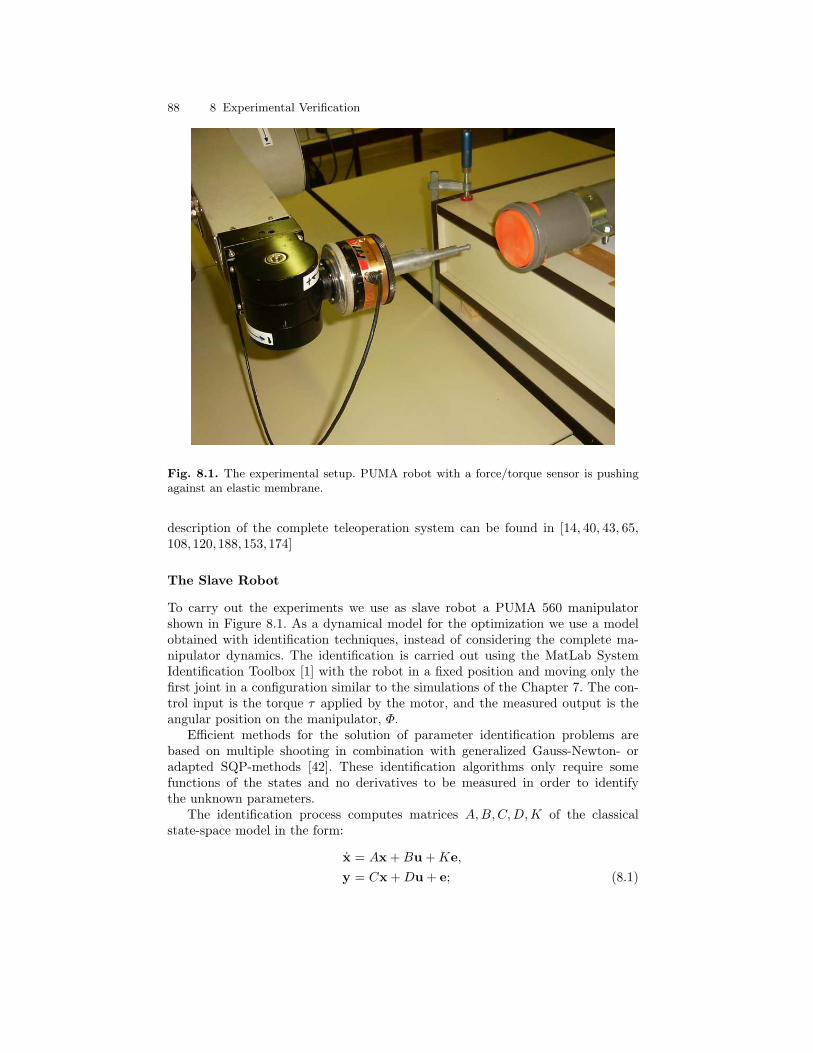
88 8 Experimental Verification
Fig. 8.1. The experimental setup. PUMA robot with a force/torque sensor is pushingagainst an elastic membrane.
description of the complete teleoperation system can be found in [14, 40, 43, 65,108,120,188,153,174]
The Slave Robot
To carry out the experiments we use as slave robot a PUMA 560 manipulatorshown in Figure 8.1. As a dynamical model for the optimization we use a modelobtained with identification techniques, instead of considering the complete ma-nipulator dynamics. The identification is carried out using the MatLab SystemIdentification Toolbox [1] with the robot in a fixed position and moving only thefirst joint in a configuration similar to the simulations of the Chapter 7. The con-trol input is the torque τ applied by the motor, and the measured output is theangular position on the manipulator, Φ.
Efficient methods for the solution of parameter identification problems arebased on multiple shooting in combination with generalized Gauss-Newton- oradapted SQP-methods [42]. These identification algorithms only require somefunctions of the states and no derivatives to be measured in order to identifythe unknown parameters.
The identification process computes matrices A,B,C,D,K of the classicalstate-space model in the form:
x = Ax +Bu +Ke,
y = Cx +Du + e; (8.1)
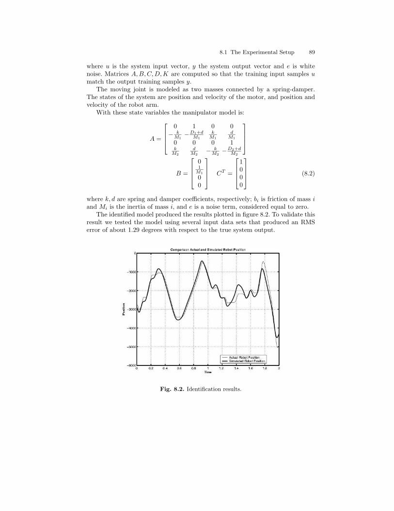
8.1 The Experimental Setup 89
where u is the system input vector, y the system output vector and e is whitenoise. Matrices A,B,C,D,K are computed so that the training input samples umatch the output training samples y.
The moving joint is modeled as two masses connected by a spring-damper.The states of the system are position and velocity of the motor, and position andvelocity of the robot arm.
With these state variables the manipulator model is:
A =
0 1 0 0
− kM1
−D1+dM1
kM1
dM1
0 0 0 1kM2
dM2
− kM2
−D2+dM2
B =
01M1
00
CT =
1000
(8.2)
where k, d are spring and damper coefficients, respectively; bi is friction of mass iand Mi is the inertia of mass i, and e is a noise term, considered equal to zero.
The identified model produced the results plotted in figure 8.2. To validate thisresult we tested the model using several input data sets that produced an RMSerror of about 1.29 degrees with respect to the true system output.
Fig. 8.2. Identification results.
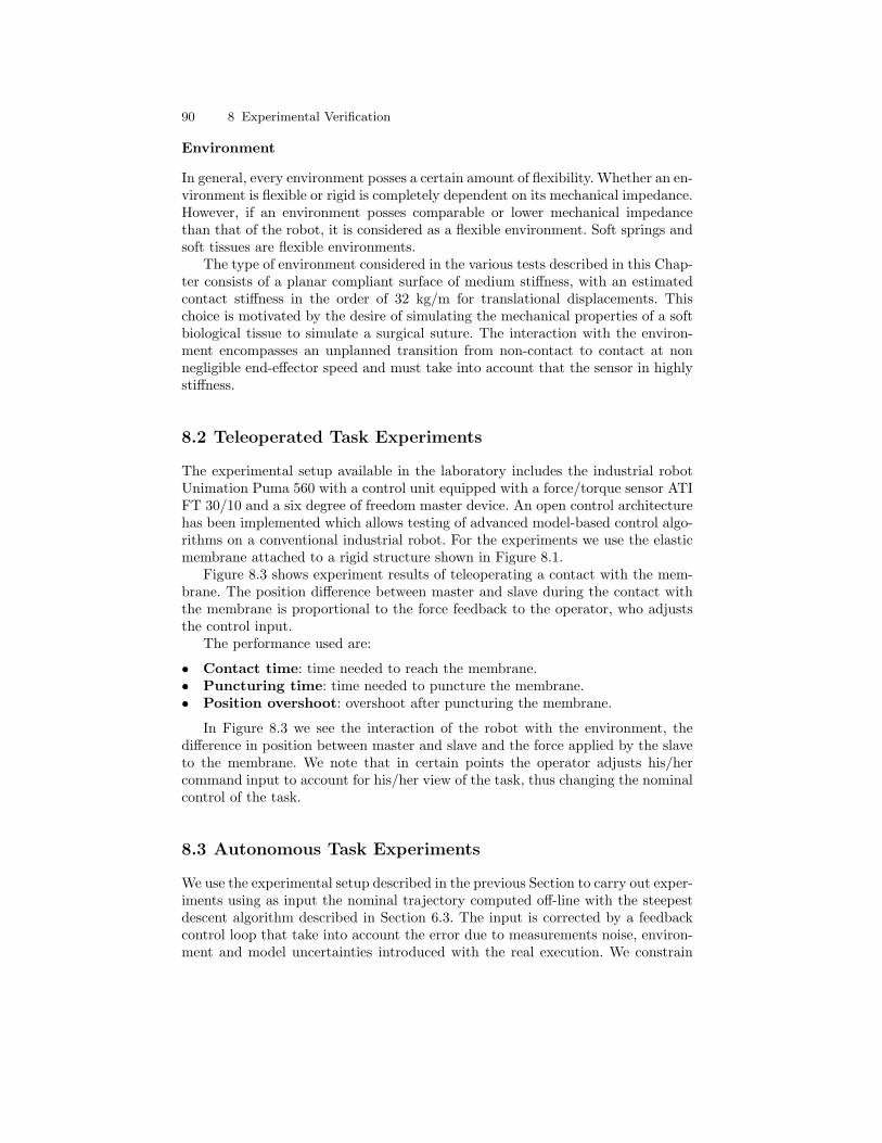
90 8 Experimental Verification
Environment
In general, every environment posses a certain amount of flexibility. Whether an en-vironment is flexible or rigid is completely dependent on its mechanical impedance.However, if an environment posses comparable or lower mechanical impedancethan that of the robot, it is considered as a flexible environment. Soft springs andsoft tissues are flexible environments.
The type of environment considered in the various tests described in this Chap-ter consists of a planar compliant surface of medium stiffness, with an estimatedcontact stiffness in the order of 32 kg/m for translational displacements. Thischoice is motivated by the desire of simulating the mechanical properties of a softbiological tissue to simulate a surgical suture. The interaction with the environ-ment encompasses an unplanned transition from non-contact to contact at nonnegligible end-effector speed and must take into account that the sensor in highlystiffness.
8.2 Teleoperated Task Experiments
The experimental setup available in the laboratory includes the industrial robotUnimation Puma 560 with a control unit equipped with a force/torque sensor ATIFT 30/10 and a six degree of freedom master device. An open control architecturehas been implemented which allows testing of advanced model-based control algo-rithms on a conventional industrial robot. For the experiments we use the elasticmembrane attached to a rigid structure shown in Figure 8.1.
Figure 8.3 shows experiment results of teleoperating a contact with the mem-brane. The position difference between master and slave during the contact withthe membrane is proportional to the force feedback to the operator, who adjuststhe control input.
The performance used are:
• Contact time: time needed to reach the membrane.• Puncturing time: time needed to puncture the membrane.• Position overshoot: overshoot after puncturing the membrane.
In Figure 8.3 we see the interaction of the robot with the environment, thedifference in position between master and slave and the force applied by the slaveto the membrane. We note that in certain points the operator adjusts his/hercommand input to account for his/her view of the task, thus changing the nominalcontrol of the task.
8.3 Autonomous Task Experiments
We use the experimental setup described in the previous Section to carry out exper-iments using as input the nominal trajectory computed off-line with the steepestdescent algorithm described in Section 6.3. The input is corrected by a feedbackcontrol loop that take into account the error due to measurements noise, environ-ment and model uncertainties introduced with the real execution. We constrain
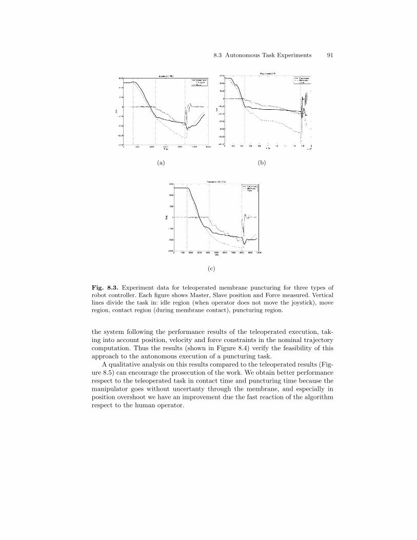
8.3 Autonomous Task Experiments 91
(a) (b)
(c)
Fig. 8.3. Experiment data for teleoperated membrane puncturing for three types ofrobot controller. Each figure shows Master, Slave position and Force measured. Verticallines divide the task in: idle region (when operator does not move the joystick), moveregion, contact region (during membrane contact), puncturing region.
the system following the performance results of the teleoperated execution, tak-ing into account position, velocity and force constraints in the nominal trajectorycomputation. Thus the results (shown in Figure 8.4) verify the feasibility of thisapproach to the autonomous execution of a puncturing task.
A qualitative analysis on this results compared to the teleoperated results (Fig-ure 8.5) can encourage the prosecution of the work. We obtain better performancerespect to the teleoperated task in contact time and puncturing time because themanipulator goes without uncertanty through the membrane, and especially inposition overshoot we have an improvement due the fast reaction of the algorithmrespect to the human operator.
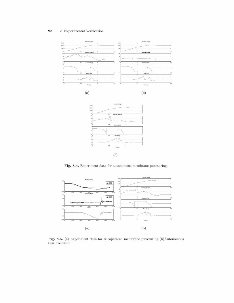
92 8 Experimental Verification
0 0.5 1 1.50
1000
2000
3000Position (step)
0 0.5 1 1.5−10
0
10
20Velocity (step/s)
0 0.5 1 1.5−2
0
2Control (Volt)
0 0.5 1 1.5−1
0
1
2Force (Kg)
Time (s)
(a)
0 0.5 1 1.50
1000
2000
3000Position (step)
0 0.5 1 1.5−50
0
50
100Velocity (step/s)
0 0.5 1 1.5−2
0
2Control (Volt)
0 0.5 1 1.5−1
0
1
2Force (Kg)
Time (s)
(b)
0 0.5 1 1.50
1000
2000
3000Position (step)
0 0.5 1 1.5−20
0
20
40Velocity (step/s)
0 0.5 1 1.5−2
0
2Control (Volt)
0 0.5 1 1.5−1
0
1
2Force (Kg)
Time (s)
(c)
Fig. 8.4. Experiment data for autonomous membrane puncturing.
0 2000 4000 6000 8000 10000 12000−5000
0
5000Position (step)
MasterSlave
0 2000 4000 6000 8000 10000 12000−100
0
100
200Velocity (step/s)
MasterSlave
0 2000 4000 6000 8000 10000 12000−2000
−1000
0
1000Force
(a)
0 0.5 1 1.50
1000
2000
3000Position (step)
0 0.5 1 1.5−10
0
10
20Velocity (step/s)
0 0.5 1 1.5−2
0
2Control (Volt)
0 0.5 1 1.5−1
0
1
2Force (Kg)
Time (s)
(b)
Fig. 8.5. (a) Experiment data for teleoperated membrane puncturing (b)Autonomoustask execution.
8.4 Conclusions 93
8.4 Conclusions
In this Chapter we have presented experiments task of puncturing a membrane asa representative surgical task. The experiments were first carried out by humansto tune the system and to generate a performance baseline against which evaluatethe autonomous execution. To this goal we defined a set of performance measuresand identified a range of ’good’ values of human performance.
Autonomous execution was carried out using the nominal controls computedoff-line following the algorithm presented in Chapter 6. According to the perfor-mance measure selected, the autonomous controller and the teleoperated task aresimilar in the executions and the autonomous execution has better performance.

9
Summary and Recomandation for FutureResearch
The most exciting phrase to hear in science, the one that heralds new discoveries, is not’Eureka!’ (I found it!) but ’That’s funny....
Isaac Asimov
In this Thesis we have developed a novel approach for the modellization, anal-ysis and execution of complex tasks, based on the formalism of Hybrid SystemTheory. The approach has been used to model, simulate and experimentally verifya simple surgical task, a suture, which includes, in a small context, most of thedifficulties of autonomous task execution. To our knowledge, the enhancement ofteleoperation using hybrid automaton has not been done so far, and the resultsof the experiments show the significance of the enhancements supported by thisapproach, since it provides a unified framework for modeling, formal verification,and testing of the execution of sequences of elementary tasks.
A new quality measure of task execution is introduced to monitor the progressof the task. Performance is evaluated only at discrete jumps between task phases,which summarize the history of the continuous portion of the hybrid system.
Dynamic Optimization has been adapted to the computation of the nominalcontrols for the task execution, and a direct numerical method has been usedto compute the nominal trajectory that satisfies the dynamics of the robot andsatisfies the constraints of task environment.
The combination of Hybrid System formalism and of the Dynamic Optimiza-tion has lead to an algorithm for the computation of the safe execution of a complextask. First, the model of the task is structured, based on a priori knowledge of thetask, and task requirements are represented as constraints on the hybrid model,either on the continuous or on the discrete states. Then an optimal trajectory, sat-isfying task constraints is computed using the Dynamic Optimization. Task qualityis measured at each discrete state, providing for warning in case of performancedegradation either in the case of autonomous or in the case of human assistedexecution.
The approach is first validated in computer simulations, which indicate thefeasibility of this approach.
96 9 Summary and Recomandation for Future Research
The experimental verification of the proposed approach is based on the teleop-eration equipment available in the Altair robotics laboratory and it consists in a6-DOF manipulator and a 1-DOF force feedback joystick and an open architectureCorba based.
9.1 Contributions
The major contributions of this Thesis can be summarized as follows.
• The problem of the autonomous execution of a complex task has been for-mulated as a Hybrid Automaton optimization, with applications to the robotassisted execution of surgical procedures.
• An in depth review of the state of the art of autonomous task execution hasbeen produced.
• A method to formalize a complex task using hybrid system tools has beenoutlined, yielding a representation of task phases, environment constraints,and quality measures.
• The concepts of Safety and Stability for complex task has been introduced,which is considered in the optimal control design.
• Pontryagin’s Maximum Principle has been adapted to the computation of op-timal hybrid trajectories, and the relative necessary conditions have been de-rived.
• Autonomous task execution has been formulated as the computation of theoptimal trajectory in space state of a hybrid automaton, and subject to statedependent constraints.
• The numerical gradient procedure for computing the time optimal solution hasbeen adapted to the hybrid system formalism, and implemented.
• This approach has combined hybrid system analysis with dynamic optimiza-tion.
9.2 Recommendations for Future Research
The following subjects are suggested for further research:
1. Hybrid System:• The development of automatic procedures for the automatic representation
of a task model, given a task execution, for example, by a skilled operator.• Development of more complex and structured task quality measures, that
can provide real time warnings on the insurgence of critical situations.• The development and analysis or different real time execution environments
and control suitable for HS.• Lesser reliance on a priori knowledge.
2. Dynamic Optimization:• The numerical computation of optimal trajectories is an important issue.
It should be made fast enough so that it could be integrated into a realtime execution system. Furthermore, different numerical algorithms should
9.3 Conclusion 97
be investigated to determine the most appropriate method for this specificoptimization problem.
3. Complete Algorithm:• Fault Recognition and Fault Recovery should be investigated and imple-
mented in the algorithm.• More complex automa should be considered.
4. Validation and Verification:• Application of Formal Methods to verify and validate the model, i.e. model
checking techniques.
9.3 Conclusion
This Thesis has developed three main aspects of autonomous execution of complextasks: the formalization of a task as a hybrid automaton, the adaptation of neces-sary optimality conditions to the case of hybrid automaton, and the developmentof a numerical procedure for the computation of the nominal task trajectory.
The Hybrid System Formalism is very suitable and powerful to represent thestructure and the constraints of a complex task. Certain features of Hybrid Sys-tems, e.g. safe sets, can be interpreted in the context of autonomous tasks, andallow high level analysis of task properties and quality. The use of a priori knowl-edge of the task allows to avoid the curse of dimensionality of hybrid systemanalysis and to compute the optimal solution in short time. When initial analysisand simulation verification is needed, the off-line computation of the optimal tra-jectory yields a nominal trajectory that can be used to verify task sequence andorganization. When the task is to be executed on a hardware system, the addi-tion of a simple feedback controller, allows the easy transition from simulation toexperimental verification.
Dynamic optimization is well suited to solve a Hybrid System planning andexecution problem, and to explore the effects of the various constraints on thefinal solution. The selection of the parameters in the numerical optimization is atool that can be used to examine the relative weight of the task constraints. Thecareful adjustment of the parameters allows the computation of different solutionsthat give a better understanding of the underlying solution space.
Finally, by combining Hybrid System formalism with Dynamic Optimizationmethods, the result is the computation of a feasible optimal trajectory that can bedirectly validated in simulation and tested with experiments. The lack of accuratemodels in certain phases of the task is compensated by the dynamic optimization.Similarly, the use of feedback control during task experiments, compensates forsome of the uncertainties not accounted for in the optimization algorithm. Al-though still in its infancy, the combination of fast heuristics hybrid system mod-eling and dynamic optimization has demonstrated its power in computing thecontrols and the sensory conditions for the autonomous execution of a complexsurgical task.

References
1. Matlab identification toolbox. The Mathworks Inc. http:www.mathworks.com.
2. Computers and Intractability: A Guide to the Theory of NPCompleteness. SanFrancisco, 1979.
3. Numerical Recipes in C. Press Syndicate, 1988.4. Applied Nonlinear Control. Prentice-Hall, 1991.5. Discrete Event Systems, Modeling and Performance Analysis. Richard D. Irwin,
Inc. The Aksen Associates Series in Electrical and Computer Engineering, Illinois,burr ridge edition, 1993.
6. Nonlinear Systems. Prentice-Hall, 1996.7. Air traffic automation: a case study in distributed decentralized control. Springer,
1998.8. J. Albro and J. Bobrow. Optimal motion primitives for a 5 dof experimental hopper.
Seoul, Korea, 2001. IEEE International Conference on Robotics and Automation.9. P. Althaus and H. Christensen. Automatic map acquisition for navigating in domes-
tic environments. In IEEE International Conference on Robotics and Automation,pages 1551–1556, Taipei, Taiwan, September 14-19 2003.
10. R. Alur, C. Courcoubetis, N. Halbwachs, T.A. Henzinger, P-H. Ho, X. Nicollin,A. Oliviero, J. Sifakis, and S. Yovine. The algorithmic analysis of hybrid systems.Theoretical and Computer Science, 138:3–34, 1995.
11. R. Alur, C. Courcoubetis, T.A. Henzinger, and P-H Ho. Hybrid automata: analgorithmic approach to the specification and verification of hybrid systems. InLecture Notes in Computer Science [94].
12. R. Alur and D. Dill. The theory of timed automata. In Theoretical and ComputerScisnce, volume 126, 1994.
13. R. Alur, T.A. Henzinger, and Sontag. Hybrid systems iii, verification and control.In Lecture Notes in Computer Science, volume 1066. Springer, 1996.
14. R.J. Anderson and W Spong. Asymptotic stability for force reflecting teleoperatorswith time delay. Journal of Robotics Research, 11(2):135–148, April 1992.
15. R. Andre-Obrecht. A new statistical approach for the automatic segmentationof continuous speeech signals. IEEE Transactions on Acustics Speech and SignalProcessing, 36(1), 1988.
16. P. Antsaklis, W. Kohn, A. Nerode, and S. Sastry. Hybrid systems ii. In LectureNotes in Computer Science. Springer, 1995.
17. P. Antsaklis, W. Kohn, A. Nerode, and S. Sastry. Hybrid systems iv. In LectureNotes in Computer Science. Springer, 1997.
100 References
18. P. Antsaklis, W. Kohn, A. Nerode, and S. Sastry. Hybrid systems v. In LectureNotes in Computer Science. Springer, 1998.
19. K. Arras, R. Philippsen, N. Tomatis, M. de Battista, M. Schilt, and R. Siegwart. Anavigation framework for multiple mobile robots and its applicaiton at the Expo02Exhibition. In IEEE International Conference on Robotics and Automation, pages1992–1997, Taipei, Taiwan, September 14-19 2003.
20. J. Azinheira, P. Rives, J. Carvalho, G. Silveira, E. de Paiva, and S. Bueno. Vi-sual control for the hovering of an outdoor robotic airship. In IEEE InternationalConference on Robotics and Automation, pages 2787–2792, Washington, DC, May2002.
21. G. Backes, P. Rabideau, K. Tao, and S. Chien. Automated planning and schedulingfor planetary rover distributed operations. In IEEE Int. Conf. on Robotics andAutomation, pages 1096–1101, Detroit,MI, May 1999.
22. P. Backes, J. Beahan, and B. Bon. Interactive command building and sequencingfor supervisory autonomy. In IEEE Int. Conf. on Robotics and Automation, pages795–801, 1993.
23. P. Backes and M. Long. Merging concurrent behaviors on a redundant manipulator.In IEEE Int. Conf. on Robotics and Automation, pages 638–645, 1993.
24. P. Backes, M. Long, and R. Steele. The modular telerobot task eecution system forspace telerobotics. In IEEE Int. Conf. on Robotics and Automation, pages 524–329,1993.
25. P. Backes and K. Tao. Umi: An interactive supervisory and shared control systemfor telerobotics. In IEEE Int. Conf. on Robotics and Automation, pages 1096–1101,1990.
26. T. Balch and R. Arkin. Behavior-based formation control for multirobot teams.IEEE Transactions of Robotics and Automation, 14(6):926–939, December 1998.
27. A. Banerjee, P. Banerjee, T. DeFanti, A. Hudson, B. Dodds, and J. Curtis. Abehavioral layer architecture for telecollaborative virtual manufacturing operations.IEEE Transactions of Robotics and Automation, 16(3):218–227, June 2000.
28. M. Basseville. Detecting chages in signals and systems - a survey. Automatica,24(3), 1988.
29. G. Bekey, H. Liu, R. Tomovich, and W. Karplus. Knowledge based control of grasp-ing in robot hands using heuristics from human motor skills. IEEE Transactions ofRobotics and Automation, 9(6):709–722, December 1993.
30. G. Bekey and R. Tomovich. Robot control by reflex action. In IEEE InternationalConference on Robotics and Automation, pages 240–247, San Francisco, CA, April7-10 1986.
31. R. Bellman. Dynamic Programming. Princeton University Press, New Jersy, 1957.32. R. Bellman. Adaptive Control Processes, A Giuded Tour. Princeton University
Press, New Jersy, 1961.33. R. Bellman and G. Leitman. On the Determination of Optimal Trajectories Via Dy-
namic Programming. Academic Press, New York, optimization techniques edition,1962.
34. R. E. Bellman, H. H. Kagiwada, R. E. Kalaba, and R. Vasudevan. Numerical analy-sis: Quasilinearization and the estimation of differential operators from eigenvalues.Commun. ACM, 11(4):255–256, 1968.
35. A. Bemporad, F. Borelli, and M. Morari. Optimal controllers for hybrid systems:Stability and piecewise linear explicit form. In 39th IEEE Conf. On Decision andControl, pages 1810–1815, Dec. 2000.
36. A. Bemporad, G. Ferrari-Trecate, and M. Morari. Observability and controllabilityof piecewise af ne and hybrid systems. IEEE Transactions on Automatic Control,45(10):1864–1876, 2000.
References 101
37. A. Bemporad and M. Morari. Control of systems integrating logic, dynamics, andconstraints. Automatica, 35(3):407–427, 1999.
38. A Benveniste. Compositional and uniform modeling of hybrid systems. IEEE Trans-actions on automatic control, Special Issue on Hybrid Systems, 1998.
39. C. Bernard, H. Kang, S. Singh, and J. Wen. Robotic system for collaborativecontrol of minimally invasive surgery. Industrial Robot: an International Journal,26(6):476–484, 1999.
40. C. Bernard, H. Kang, S.K. Singh, and Wen J.T. Robotic system for collaborativecontrol in minimally invasivesurgery. Industrial Robot:An international Journal,26(6):476–484, 1999.
41. A. et al. Bicchi. A sensorized minimally invasive surgery tool for detecting tissueelastic properties. In 1996 IEEE International Conference on Robotics and Automa-tion:, 1996.
42. H.G. Bock, E. Eich, and J.P. Schloder. Numerical solution of constrained leastsquares boundary value problems in differential-algebraic equations. In K. Strehmel,editor, Numerical Treatment of Differential Equations.
43. D. Botturi, A. Castellani, D. Moschini, and P. Fiorini. Performance evaluation oftask control in teleoperation. In International Conference on robotics and Automa-tion, New Orleans, 2004.
44. M. S. Branicky, V. S. Borkar, and S. K. Mitter. A unified framework for hybridcontrol: Model and optimal optimal control theory. IEEE Transaction on AutomaticControl, 43(1):31–45, April 1998.
45. M.S. Branicky. Topology of hybrid systems. In 32nd IEEE CDC, pages 2309–2314,San Antonio,TX, december 1993.
46. M.S. Branicky. Multiple lyapunov functions and other analysis tools for switchedand hybrid systems. IEEE TRansaction on Automatic Control, 43(4), 1998.
47. M.S. Braniky. Universal computation and other capabilities of hybrid and contin-uous dynamical systems. Theoretical Computer Science, 138(1):67–100, 1995.
48. R. Brockett. Hybrid systems in classical mechanics. In 13th IFAC, pages 473–476,1996.
49. R.W. Brockett. Hybrid models for motion control systems. In H.L. Tentleman andJ.C. Willems, editors, Essays on Control: Perspectives in Theory and its Applica-tions, Boston, 1993. Birkhauser.
50. R. Brooks. A robust layered control system for a mobile robot. IEEE Transactionsof Robotics and Automation, 2(1), 1986.
51. R. Brooks. A hardware retargetable distribuited layered architecture for mobilerobot control. In IEEE International Conference on Robotics and Automation,pages 240–247, Raleigh, NC, March 31 - April 3 1987.
52. A.E. Bryson and W.F. Denham. A steepest ascent method for solving optimumprogramming problems. J.Applied Machanics, (29):247–57, 1962.
53. A.E. Bryson and Yu-Chi Ho. Applied Optimal Control. Hemisphere PublishingCorporation, 1975.
54. D. Bullock and S. Grossberg. A neural network architecture for automatic tra-jectory formation and coordination of multiple effectors during variable-speed armmovements. In IEEE International Conference on Neural Network, pages 559–566,San Diego, CA, June 1987.
55. M. Buss, O. Von Stryk, R. Bulirsch, and G. Schmidt. Towards hybrid optimalcontrol. Technical report, University of Berlin, 2000.
56. P.E. Caines and Y-J. Wei. Hierarchical hybrid control systems: A lattice formula-tion. Transactions on Automatic Control, Special Issue on Hybrid Systems, 1998.
57. M. Campos, G. Pereira, S. Vale, A. Bracarense, G. Pinheiro, and M. Oliveira. Amobile manipulator fo rinstallation and removal of aircraft warning spheres on aerial
102 References
power transmission lines. In IEEE International Conference on Robotics and Au-tomation, pages 3559–3564, Washington, DC, May 2002.
58. C. Cao, C. MacKenzie, and S. Payandeh. Task and motion analyses in endoscopicsurgery. In ASME IMECE Conference: 5th Annual Symposium on Haptic Interfacefor Virtual Environment and Teleoperator Systems, pages 583–590, Atlanta,GA,1996.
59. C. Casadei, S. Martelli, and P. Fiorini. A workcell for the development of robot-assisted surgical procedures. Journal of Intelligent and Robotic Systems, (28):301–324, 2000.
60. A. Castellani, D. Botturi, M. Bicego, and P. Fiorini. Hybrid hmm/svm model for theanalysis and segmentation of teleoperation tasks. In IEEE International Conferenceon Robotics and Automation, New Orleans,LA, 2004.
61. M. C. Cavusoglu, J. Yan, and S. S. Sastry. A hybrid system approch to contactstability and force control in robotic manipulator. In 12th IEEE InternationalSymposium on Intelligent Control, pages 143–148, July 1997.
62. L. Chaimowicz, M. Campos, and V. Kumar. Dynamic role assigment for cooperativerobots. In IEEE International Conference on Robotics and Automation, pages 293–298, Washington, DC, May 2002.
63. L. Chaimowicz, M. Campos, and V. Kumar. Hybrid systems modeling of cooperativerobots. In IEEE International Conference on Robotics and Automation, pages 4086–4091, Taipei, Taiwan, September 2003.
64. Z. Chaochen, A.P. Ravn, and M.R. Hansen. An extended duration calculus forhybrid real-time systems. In Lecture Notes in Computer Science [94].
65. S. Charles, H. Das, T. Ohm, C. Boswell, G. Rodriguez, R. Steele, and D. Istrate.Dexterity-enhanced telerobotics microsurgery. In 8th International Conference onAdvanced Robotics (ICAR97), Monterey, CA, July 1997.
66. R. Courant and D. Hilbert. Methods of Methematical Physics, volume 1. Inter-science, New York, 1953.
67. J.E.R. Cury, B.H. Krogh, and T. Niinomi. Synthesis of supervisory controllersfor hybrid systems based on approximating automata. Transactions on AutomaticControl, Special Issue on Hybrid Systems, 1998.
68. H. Das, H. Zak, W. S. Kim, A. K. Bejczy, and P. S. Schenker. Operator performancewith alternative manual control modes in teleoperation. Presence, 1(2):201–218,Spring 1992.
69. B. Davies. A review of robotics in surgery. volume Part H, pages 129–140. Institutionof Mechanical Engineers, 2000.
70. B. De Schutter. Optimal control of a class of linear hybrid systems with saturation.SIAM Journal on Control and Optimization,, 2000.
71. K.T Den Boer. Surgical Task Performance, Assessment using Time-Action Analy-sis. PhD thesis, Delft University of Technology, 2001.
72. A.M. Derossis, G.M. Fried, M. Abrahamowicz, H.H. Sigman, J.S. Barkun, and J.L.Meakins. Development of a model for training and evaluation of laparoscopic skills.Am.J.Surg, 1998.
73. A. Deshpande, A. Gollu, and P. Varaiya. The shift programming language andrun-time system for dynamic networks of hybrid automata. IEEE Transactions onautomatic control, Special Issue on Hybrid Systems, 1998.
74. A. Deshpande and P. Varaiya. Viable control of hybrid systems. In 35th IEEEConference on Decision and Control, Kobe, Japan.
75. The Galileo development team. Galileo program description document: commandand data subsystem. Technical Report 625-355-060000, D-535 Rev. G, NASA JetPropulsion Laboratory, California Institute of Technology, Pasadena, CA (USA),May 1989.
References 103
76. M.B. Dias, M. Zinck, R. Zlot, and A. Stentz. Robust multirobot coordination indynamic environments. In IEEE International Conference on Robotics and Au-tomation, pages 3435–3441, New Orleans, LA, April 2004.
77. P. M. Do Carmo. Differential Geometry of Curves and Surfaces. Prentice-Hall,Upper Side river, New Jersey, 1976.
78. M. Dogruel, S. Drakunov, and Ozguner. Sliding mode control in discrete statesystems. In 32nd Conference on Decision and Control, pages 1194–1199, 1993.
79. S.E. Dreyfus. Dynamic Programming and the Calculus of Variations. AcademicPress, New York, 1965.
80. R. Dubey, S. Everett, N. Pernalete, and K. Manocha. Teleoperation assistancethrough variable velocity mapping. IEEE Transactions of Robotics and Automation,17(5):761–766, October 2001.
81. B. Eberman. A model-based approach to cartesian manipulation contact sensing.International Jurnal of Robotics Research, 16(4), 1997.
82. B. Eberman and J.K. Salisbury. Application of change detection to dynamic contactsensing. International Jurnal of Robotics Research, 13(5), 1994.
83. M. Egerstedt. Behavior based robotics using hybrid automata. In Springer-Verlag,editor, Lecture Notes in Computer Science: Hybrid Systems III, pages 103–116. 2000.
84. A. Ferreira. Strategies for human robot interaction for automatic microassembly.In IEEE International Conference on Robotics and Automation, pages 3076–3081,Taipei, Taiwan, September 2003.
85. P.A. Finlay and M.H. Ornstein. Controlling the movement of a surgical laparoscope.IEEE Engineeing in Medicine and Biology, pages 289–291, May/June 1995.
86. P. Fiorini. Autonomous organization of grasping tasks. In SPIE Symposia onAerospace Sensing, Artificial Intelligence VII, Orlando, FL, March 27-31 1989.
87. P. Fiorini, A. Giancaspro, S. Losito, and G. Pasquariello. Neural networks for thesegmentation of teleoperation tasks. In Presence, pages Vol.2, Number I, Winter1993.
88. P.M. Fitts. The information capacity of the human motor system in controlling theamplitude of movements. Journal of Experimental Psychology, 47(6):381–391, June1954.
89. A.F. Fuller. Lyapunov centenary issue. International Journal of Control, 55(3),1992.
90. I.M. Gelfand and S.V. Fomin. Calculus of Variations, volume 1. Prentice-Hall, NewJersy, 1963.
91. P. Gill, W. Murray, and M. Saunders. Users guide for SNOPT 5.3: a fortranpackage for large-scale nonlinear programming. Department of Mathematics, Univ.of California, San Diego, 1997.
92. A. Gollu and P. Varaiya. Hybrid dynamical systems. In 28th IEEE Conference onDecision and Control, pages 2708–2712, Tampa, Florida, December 1989.
93. G. Grammel. Maximum principle for hybrid system via singular pertrubations.SIAM Control and Optimization, 37(4):1162–1175, 1999.
94. A. Grossman, A. Nerode, A.P. Ravan, and H. Rischel. Hybrid systems. In LectureNotes in Computer Science, volume 736. Springer-Verlag, 1993.
95. J. Guckenheimer. A robust hybrid stabilization strategy for equilibria. IEEE Trans-actions on Automatic control, 40(2):321–326, 1995.
96. A. Guia, C. Seatzu, and C. V. D. Mee. Optimal control of switched autonomouslinear systems. In 40th IEEE Conf. On Decision and Control, pages 2472–2477,Dec. 2000.
97. B. Hannaford and P. Lee. Hidden markov model analysis of force/torque informationin telemanipulatio. The International Journal of Robotics Research, 10(5):528–539,October 1991.

104 References
98. M. Hardt, J. Helton, and K. Kreutz-Delgado. Numerical solution of nonlinear h2 andh1 control problems with application to jet engine compressors. IEEE Transactionson Control Systems Technology, 2000.
99. S. Hayati, T. Lee, K. Tso, and P. Backes. A testbed for a unified teleoperated-autonomous dual-arm robotic system. In IEEE Int. Conf. on Robotics and Au-tomation, pages 1090–1095, 1990.
100. S. Hayati, T. Lee, K. Tso, P. Backes, and E. Kan. The jpl telerobot manipulatorcontrol and mechanization subsystem (mcm). pages 173–181.
101. S. Hedlund and A Rantzer. Optimal control of hybrid systems. In 38th IEEE Conf.On Decision and Control, pages 3972–3977, Dec 1999.
102. W.P.M.H. Heemels, J.M. Schumacher, and S. Weiland. Linear complementaritysystems. SIAM Journal on Applied Mathematics, 60(4):1234–1269, 2000.
103. T. Henderson et al. The specification of distributed sensing and control. Journalof Robotic Systems, 2(4), April 1985.
104. T.A. Henzinger, P-H. Ho, and H. Wong-Toi. Algorithmic analysis of nonlinearhybrid systems. IEEE Transactions on automatic control, Special Issue on HybridSystems, 1998.
105. I.A. Hiskens. Analysis tools for power systems - contending with nonlinearities.1995.
106. R.D. Howe and Y. Matsuoka. Robotics for surgery. In Annual Review of BiomedicalEngineering, volume 1. 1999.
107. M. Johansson and A. Rantzer. Computation of piecewise lyapunov function forhybrid systems. IEEE Transaction on Automatic Control, 43(4):555–559, April1998.
108. H. Kang and J.T. Wen. Robotic assistants aid surgeons during minimally inva-sive procedures. IEEE Engineering in Medicine and Biology, pages 94–104, Jan-uary/February 2001.
109. L.V. Kantorovich and V.I. Krylov. Approximate Methods of Higher Analysis, vol-ume 1. Interscience and P.Noordhoff Ltd., New York and Groningen, The Nether-lands, 1958.
110. H.J. Kelley and G. Leitman. Method of Gradients. Academic Press, New York,optimization techniques edition, 1962. Chapter 6.
111. M. Kitagawa, M. Okamura, B.T. Bethea, V.L. Gott, and A. Baumgartner. Anal-ysis of suture manipulation forces for teleoperation with force feedback. In FifthInternational Conference on Medical Image Computing and Computer Assisted In-tervention (MICCAI), 2002.
112. I. Kolmanovsky and N.H. McClamroch. Hybrid feedback laws for a class of nonlinearcascade systems. IEEE Transaction on Automatic Control, 41:1271–1281, 1996.
113. K. Kondak and G. Hommel. Computation of time optimal movements for au-tonomous parking of non-holonomic mobile platforms. Seoul, Korea, 2001. IEEEInternational Conference on Robotics and Automation.
114. D. Kragic, A. Miller, and P. Allen. Realtime tracking meets on line grasping plan-ning. In IEEE International Conference on Robotics and Automation, pages 2460–2465, Seoul, Korea, May, 21-26 2001.
115. A. Krupa, C. Doignon, J. Gangloff, M. de Mathelin, G. Morel, L. Soler, J. leroy,and M. Ghodoussi. Towards semi-autonomy in laparoscopic surgery: first live ex-periments. Sant’Angelo d’Ischia, Italy, July 2002.
116. A Krupa, C. Doignon, J. Gengloff, M. de Mathelin, L. Soler, G. Morel, J. Leroy,and M. Ghodoussi. Towards semi-autonomy in laparoscopic surgery: first live ex-periment. In 8th International Symposium on Experimental Robotics, Sant’Angelod’Ischia, Italy, July 2002.

References 105
117. Y.S. Kwoh, E. Jonckheere, and S. Hayati. A robot with improved absolute position-ing accuracy for ct guided stereotactic surgery. IEEE Transaction on BiomedicalEngineering, pages 153–161, February 1988.
118. R.E. Larson. Dynamic programming with reduced computational requirements.IEEE Transaction on Automatic Control, (10):135–143, 1965.
119. J.C. Latombe, editor. Robot Motion Planning. Kluwer Academic Publisher, Boston,MA, 1991.
120. D.A. Lawrence. Stability and transparency in bilateral teleoperation. IEEE Trans-action on Robotics and Automation, 9(5):624–637, October 1993.
121. S. Lee and M.H. Kim. Cognitive contorl of dynamic systems. In IEEE InternationalSymposium on Intelligent Control, pages 455–460, Philadelphia, PA, January 19-201987.
122. G. Leitman. An Introduction to Optimal Control. McGraw-Hill Book Co., NewYork, NY, 1966.
123. M.D. Lemmon and P.J. Antsaklis. Timed automata and robust control: Can wenow control complex dynamical systems? In 36th IEEE Conference on Decisionand Control.
124. M. Lind. The use of flow models for automated plant diagnosis. In NATO Sy,posiumon human detection and diagnosis of system failures, 1981.
125. J. Lygeros, D.N. Godbole, and S. Sastry, editors. A Game Theoretic Approach toHybrid System Design. University of California, Berkeley, 1995.
126. J. Lygeros, D.N. Godbole, and S. Sastry. Multiagent hybrid system design usinggame theory and optimal control. In 35th IEEE Conference on Decision and Con-trol, pages 1190–1195, Kobe, Japan, 1996.
127. J. Lygeros, D.N. Godbole, and S. Sastry. Verified hybrid controllers for automatedvehicles. Transactions on Automatic Control, Special Issue on Hybrid Systems,1998.
128. N. Lynch, R. Segala, and F. Vaandrager. Hybrid i/o automata. Inf. Comput.,185(1):105–157, 2003.
129. H. Maa and U. Kuhnapfel. Noninvasive measurement of elastic properties of livingtissue. Technical report, Institut fr Angewandte Informatik, ForschungszentrumKarlsruhe,, 1997.
130. B. Martin and J. Bobrow. Minimum e ort motions for open chain manipulatorswith task-dependent end-e ector constraints. Albuquerque, New Mexiko, 1997. InProceedings of the IEEE International Conference on Robotics and Automation.
131. N.H. McClamroch, C. Rui, I. Kolmanvsky, and M. Reyhanoglu. Hybrid closed loopsystems: A nonlinear control perspective. In 36th IEEE Conference on Decisionand Control, 1997.
132. R. McGill. Optimal control, inequality state constraint, and the generalized newton-raphson algorithm. SIAM J.Control, 1965.
133. E.J. McShane. On Multipliers for Lagrange Problems, volume 61. American J.Math., New York, 1939.
134. W.S. Melvin and E.C Johnson, J.A.and Ellison. Laparoscopic skill enhancement.Am.J.Surg., 1996.
135. C.W. Merriam. Optimization Theory and Design of Feedback Control Systems.McGraw-Hill Book Co., New York, 1964.
136. A. Meystel. Intelligent control in robotics. Journal of Robotic Systems, 5(4):269–308, August 1988.
137. A.S. Morse. Control using logic-based switching. In Lecture Notes in Control andInformation Science, volume 222. Springer, 1997.
138. M.S.Branicky. Studies in Hybrid Systems:Modeling, Analysis, and Control. PhDthesis, Massachusetts Institute of Technology, 1995. In English.
106 References
139. A. Nerode and W. Kohn. Multiple agent hybrid control architecture. In LectureNotes in Computer Science [94].
140. K. Passino and P. Antsaklis. A system and control theoretic perspective on artificialintelligence planning systems. Applied Artificial Intelligence, 3:1–32, 1989.
141. P. Peleties and R.A. DeCarlo. Modeling of interacting continuous time and discreteevent systems: An example. In 26th Annual Allerton Conference on comunication,control and Computing, pages 1150–1159, 1988.
142. P. Peleties and R.A. DeCarlo. Asymptotic stability of m-switched systems usinglyapunov-like functions. In American Control Conference, pages 1679–1684, 1991.
143. L. Petersson, D. Austin, and D. Kragic. High-level control of a manipulator fordoor opening. volume 3, pages 2333–2338, Takamatsu, Kagawa, Japan, 2000.
144. S. Pettersson and B. Lennartson. Stability and robusteness of hybrid systems. In35th Conference on Decision and Control, Kobe, Japan, 1996.
145. A. Pnueli and J. Sifakis. Special issue on hybrid systems. In Theoretical ComputerScinence, volume 138, 1995.
146. L.S. Pontryagin. The Mathematical Theory of Optimal Processes. Wiley, New York,1962.
147. A. Potocnik, B.and Bemporad, F.D. Torrisi, G. Music, and B. Zupancic. Hysdelmodeling and simulation of hybrid dynamical systems. In MATHMOD Conference,Vienna, February 2003.
148. K. Radermacher, H.W. Staudte, and G. Rau. Computer assisted orthopaedicsurgery by means of individual templates. aspects and analysis of potential applica-tions. In 1st International Symposium on Medical Robotics and Computer AssistedSurgery (MRCAS’94), pages 42–48, Pittsburgh, PA, September 1994.
149. J. Raisch and S.D. O’Young. Discrete approximation and supervisory control ofcontinuous systems. Transactions on Automatic Control, Special Issue on HybridSystems, 1998.
150. J. Rasmussen and M. Lind. Coping with complexity. In European Annual Confer-ence of Human Decision and Manual Control, Delft, The Netherlands, 1981.
151. J. Rasmussen and M. Lind. Model of human decision making in complex systemsand its use for design of control strategies. In American Control Conference, Ar-lington, VA, June, 14-16 1982.
152. J. Rosen, J.D. Brown, L. Chang, M. Barreca, M. Sinanan, and B. Hannaford. Thebluedragon - a system for measuring the kinematics and the dynamics of minimallyinvasive surgical tools in-vivo. In 2002 IEEE International Conference on Roboticsand Automation, pages 1876–1881, Washington, DC, May 2002.
153. Jee-Hwan Ryn, Dong-Soo Kwon, and B. Hannaford. Stable teleoperation with timedomain passivity control. In 2002 IEEE International Conference on Robotics &Automation, pages 3260–3264, Waschintong, US, May 2002.
154. A.P. Sage and C.C.III White. Optimum System Control. Prentice-Hall, New Jersy,1977.
155. R. Satava. Virtual reality surgical simulator. Surg Endosc, 1993.156. R. Sengupta and S. Lafortune. An optimal control theory for discrete event systems.
SIAM Control and Optimization, 36(2):488–541, 1998.157. R. Simmons. Structured control for autonomous robots. IEEE Transactions of
Robotics and Automation, 10(1):34–43, February 1984.158. C. Simone. Modeling of needle insertion forces for percutaneous therapies. PhD
thesis, The Johns Hopkins University, Baltimore, Mariland, 2002.159. E. D. Sontag, editor. Mathematical Control Theory: Deterministic Finite Dimen-
sional Systems. Springer, New York, 1998.160. E.D. Sontag. Nonlinear regulation: the piecewise linear approach. IEEE Transac-
tions on Automatic Control, 26(2):346–357, 1981.
References 107
161. J.A. Stiver, P.J. Antsaklis, and M.D Lemmon. An invariant based approach to thedesign of hybrid contol systems. volume J, San Francisco, 1996.
162. J.A. Stiver, P.J. Antsaklis, and M.D. Lemmon. A logical des approach to the designof hybrid control systems. Mathl. Comput. Modelling, 23(11/12):55–76, 1996.
163. Y. Sun, N. Xi, and Y. Wang. Modeling and analysis of perceptive robot controllerbased on hybrid automata. In IEEE International conference on robotics and Au-tomation, New Orleans, LA, 2004.
164. G.T. Sung and I.S. Gill. Robotic laparoscopic surgery: a comparison of the da vinciand Zeus systems. Elsevier Science, Urology(58):893–898, 2001.
165. L.W. Tang, G. D’Ancona, J. Bergsland, and H.L. Kawaguchi, A.and Kara-manoukian. Robotically assisted video-enhanced-endoscopic coronary artery bypassgraft surgery. Angiology, 52:99–102, 2001.
166. L. Tavernini. Differential automata and their discrete simulator. In NonlinearAnalysis, Theory, Methods and Applications, volume 11, pages 665–683, 1987.
167. J.H. Taylor and D. Kebede. Modeling and simulation of hybrid systems in matlab.volume J, San Francisco, 1996.
168. R.H. Taylor, J. Funda, B. Eldridge, S. Gomory, K. Gruben, D. LaRose, M. Talamini,L. Kavoussi, and J. Anderson. A telerobotic assistant for laparoscopic surgery. IEEEEngineeing in Medicine and Biology, pages 279–288, May/June 1995.
169. R.H. Taylor, S. Lavalle, G.C. Burdea, and R. Mosges, editors. Computer - IntegratedSurgery. MIT Press, Cambridge, MA, 1996.
170. M. Tittus and B. Egart. Control design for integrator hybrid systems. IEEE Trans-action on Automatic Control, 43(4):491–500, April 1998.
171. C. Tomlin. Towards effcient computation of solutions to hybrid systems. Phoenix,AZ, 1999. 38th IEEE Conference on Decision and Control.
172. C. Tomlin, G.J. Pappas, and S. Sastry. Conflict resolution for air traffic manage-ment: A study in multi-agent hybrid systems. Transactions on Automatic Control,Special Issue on Hybrid Systems, 1998.
173. R. Tomovich et al. A strategy for grasp synthesis with multifingered robot hands. InIEEE International Conference on Robotics and Automation, pages 83–89, Raleigh,NC, March 31 - April 3 1987.
174. J. Troccaz, M. Peshkin, and B. Davies. The use of localizers, robots and synergisticdevices in cas. In 4th International Symposium on Medical Robotics and ComputerAssisted Surgery (CVRMed-MRCAS’97), pages 727–735, Grenoble, France, March1997.
175. University of Pennsylvania School of Veterinary Medicine. Principles of Surgery.176. A.J. Van der Schaft and M. Schumacher. Complementarity modeling of hybrid
systems. IEEE Transaction on Automatic Control, 43(4):483–490, April 1998.177. A.J. Van der Schaft and M. Schumacher. An introduction to hybrid dynamical
systems. In Springer Verlag, editor, In Lecture Notes in Control and InformationSciences, volume 251. 2000.
178. O. Von Stryk. Numerical hybrid optimal control and related topics. PhD thesis,Technical University of Munich, 2000. In English.
179. O. Von Stryk. User s guide for DIRCOL version 2.1: A direct collocation methodfor the numerical solution of optimal control problems. Tecnical University of Darm-stadt, 2001. WWW:www.sim.informatik.tu-darmstadt.de/sw/.
180. O. Von Stryk and M. Glocker. Decomposition of mixed-integer optimal controlproblems using branch and bound and sparse direct collocation. In ADPM 4th Intl Conf. on Automation of Mixed Processes: Hybrid Dynamic Systems, 2000.
181. O. Von Stryk and M. Schlemmer. Optimal control of the industrial robot manutecr3. In R. Bulirsch and D. Kraft, editors, Computational Optimal Control, volume115 of International Series of Numerical Mathematics, pages 367–382. 1994.
108 References
182. J.C. Willems. Paradigms and puzzles in the theory of dynamical systems. IEEETransactions on Automatic Control, 36:259–294, 1991.
183. A.S. Willsky. A survey of design methods for failure detection in dynamic systems.Automatica, 12(6), 1974.
184. N. Xi, Tarn T.J., and A.K. Bejczy. Intelligent planning and control for multirobotcoordination: An event-based approach. IEEE Transaction on Robotics and Au-tomation, 12(2), June 1996.
185. X. Xu and J. Antsaklis. A dynamic programmin approach for optimal control ofswitched systems. In 39th IEEE Conf. On Decision and Control, pages 1822–1827,Dec. 2000.
186. H. Ye, A.N. Michel, and L. Hou. Stability theory for hybrid dynamical systems.pages 2779–2684, New Orelans, 1995. IEEE Conference on Decision Control.
187. H. Ye, N. Michel, and L. Hou. Stability theory for hybrid dynamical systems. IEEETransaction on Automatic Control, 43(4):461–474, April 1998.
188. Y. Yokokohji and T. Yoshikawa. Bilateral control of master-slave manipulatorsfor ideal kinestetic coupling–formulation and experiment. IEEE Transactions onRobotics and Automation, 10(5):605–620, October 1994.
Sommario
La continua crescita della Chirurgia Minimamente Invasiva e motivata dallavolonta di migliorare le cure dei pazienti e contemporaneamente abbassare i costidella sanita. Questi obiettivi richiedono lo sviluppo di tecniche chirurgiche, conparticolare attenzione alla riduzione della variabilita e la crescita dell’efficienzadelle stesse.
Molti dispositivi robotici sono stati sviluppati o proposti per cercare di rag-giungere tali obiettivi, ed alcuni di essi sono usati in ambito ospedaliero. Nellarobotica assistita le procedure sono completamente eseguite dal chirurgo e il robotsvolge solamente la funzione di strumento, a volte anche troppo sofisticato, persvolgere tale operazione.
Quindi per aumentare la qualita delle cure e ridurre il loro costo, sarebbedesiderabile e necessario esplorare lo sviluppo di algoritmi che diano la capacita alrobot di collaborare con il chirurgo durante una procedura minimamente invasiva.In questo contesto, con collaborazione si intende la capacita di un robot di portareavanti autonomamente sottoprocedure, adattandosi alla forte variabilita tipica dell’ambiente chirurgico. Questa collaborazione potrebbe ridurre le fatiche del chirurgo,eliminare la variabilita presente tra i vari specializzandi e conseguentemente nellaesecuzione delle procedure chirurgiche ed infine aumentare l’efficienza dell’interosistema riducendo il tempo di impiego del chirurgo.
In questa tesi viene esaminata l’esecuzione automatica di compiti robotici inambiente non completamente conosciuto come quello chirurgico, e viene propostoun metodo per il calcolo del controllo nominale per un robot che esegue una tipicaprocedura chirurgica.
La sicurezza e un problema molto importante nella chirurgia robotica, ed e an-cora piu importante nell’esecuzione automatica ti procedure chirurgiche. I robotchirurghi attualmente in commercio non utilizzano la retroazione di forza, privandol’operatore umano di una modalita di controllo delle prestazione del robot moltopotente. Quindi, ancora oggi, una grande responsabilita per la corretta esecuzionedella procedura e messa nella correttezza dell’algoritmo di controllo, vista la vari-abilita dell’ambiente. In questa Tesi viene investigata la sicurezza dell’algoritmoutilizzando l’ottimizzazione con vincoli sull’esecuzione. La variabilita e consideratarispetto al modello del compito ed ai vincoli ed e quantificata come la distanzadel comportamento corrente del robot da quello desiderato durante un’operazioneminimamente invasiva. Questo approccio consente anche di monitorare continua-mente la qualita della procedurae le prestazioni dell’operatore.
Tradizionalmente, l’esecuzione automatica di procedure e stata affrontata sem-plificando il problema ingegnerizzando l’ambiente, ad esempio aggiungendo op-portuni punti fissi per cercare di rimuovere l’incertezza del compito. Le piu avan-zate tecniche di controllo consistono di comportamenti pre-programmati, cosı chedifferenti compiti possano essere programmati ed eseguiti usando lo stesso in-sieme di comportamenti di base. Quando non e disponibile un modello esplicitodell’ambiente, i comportamenti vengono parametrizzati in modo da consentire al-cuni gradi di flessibilita nell’esecuzione del compito. Se il compito e/o il modello
110 References
dell’ambiente sono conosciuti o possono essere identificati, e possibile sviluppareuna legge di controllo esplicita per il controllo dell’esecuzione della procedura. Inquesta Tesi abbiamo sviluppatouna legge di controllo esplicita usando le teoriadei Sistemi Ibridi, e abbiamo modellato l’incertezza con una appropiata sequanzadi stati nel sistema ibrido. In particolare, abbiamo usato un automaton deter-ministico come modello della procedura considerato che le procedure chirurgichestudiate sono ben codificate nella letteratura medica, e possono essere propiamenterappresentate come procedure autonome.
Rappresentiamo una procedura chirurgicacome un automaton ibrido i qualistati elementari rappresentanouna distinta azione della procedura. In questo modo,possiamo calcolare il controllo nominale ottimizzando un appropiato indice diqualita nel dominio del sottocompito, che corrisponde ad ogni azione del compito.In questo contesto, il compromesso tra la conoscenza esplicita del modello e la com-pensazione con retroazione influenza pesantemente le prestazioni del sistema. Ab-biamo indagato la relazione tra conoscenza a priori, rappresentata dall’automatonibrido, il numero e la forma dei vincoli ed il tipo di retroazione on-line per garantiredelle linee guida per il progetto dell’intero sistema.
Auspichiamo che l’integrazione di tecniche dalla teoria dei sistemi ibridi, dell’ottimizzazione vincolata e della rappresentazione dei vincoli, faciliti l’autonomiain ambiente incerto. Per dimostrare questo , abbiamo simulato l’esecuzione auto-matica di una sutura, che e una comoda e rappresentativa procedura chirurgica.L’esecuzione della sutura richiede la definizione di una traiettoria nominale cheguidi il robot alla completa e corretta esecuzione del compito. A questo riguardo,definiamo una strategia ottima per calcolare la traiettoria ottima off-line ed unacompensazione on-line dalla deviazione dalla traiettoria ottima. Possiamo con-cludere che l’integrazione di metodi diversi come sistemi ibridi, metodi di ottimiz-zazione e controllo ottimo hanno facilitato la costruzione di una piu sicura ese-cuzione automatica di una realistica procedura chirurgica.
Riassumendo, un insieme di strumenti per la sintesi del controllo un un compitocomplesso e stato proposto, investigato e valutato nel contesto delle procedurechirurgiche autonome. Questo metodo sviluppato costituisce una ricca base pertrattare compiti complessi in ambiente non conosciuto ed espande la parte sullostato dell’arte dell’esecuzione automatica di compiti.
Copyright © 2022 FDOKUMEN