---

Available online al www.sciencedirect.com -" INFORMATION ..:;, ScienceDirect SCIENCES

AN INTERNATIONAl J0I;RNAL

Information Sciences 177 (2007) 2075-2098

www.elsevier.com/locate/ins ELSEVIER

Human evolutionary model: A new approach to optimization

Osear Montiel a, Osear Castillo b,*, Patricia Melin b, Antonio Rodríguez Díaz e,

Roberto Sepúlveda a

a CITEDI-IPN, Av. del Parque #1310, Mesa de Otay Tijuana, BC, Mexico b Department oi Computer Science, Tijuana Institute oi Technology, P. O. Box 4207, Chula Vista, CA 91909, USA

e FCQI-UABC Tijuana, BC, Mexico

Received 15 September 2006; accepted 21 September 2006

Abstract

The aim of this paper is to propose the Human Evolutionary Model (HEM) as a novel eomputational method for solv­ing seareh and optimization problems with single or multiple objeetives, HEM is an intelligent evolutionary optimization method that uses eonsensus knowledge from experts with the aim of inferring the most suitable parameters to aehieve the evolution in an intelligent way, HEM is able to handIe experts' knowledge disagreements by the use of a novel eoneept eal1ed Mediative Fuzzy Logic (MFL). The effeetiveness of this computational method is demonstrated through several experiments that were performed using c1assieal test funetions as wel1 as eomposite test functions. We are eomparing our results against the results obtained with the Genetie Algorithm of the Matlab's Toolbox, Evolution Strategy with Covarianee Matrix Adaptation (CMA-ES), Particle Swarrn Optimizer (PSO), Cooperative PSO (CPSO), G3 model with PCX erossover (G3-PCX), Differential Evolution (DE), and Comprehensive Learning PSO (CLPSO). The results obtained using HEM outperforms the results obtained using the abovementioned optimization methods. © 2006 Elsevier lne. AH rights reserved.

Keywords: HEM; Intelligent evolutionary algorithm; Optimization; Fuzzy adaptation

1. Introduction

Estimating optimal solutions for real-world problems such as finding the maximal possible reliability in the design of a product comprised with reducing its cost, modeling a physical system, or others, has become a

, necessity since there is no standard and infallible technique. Recently, optimization has received enormous attention as a direct consequence of the rapid progress in computer technology inc1uding the availability of powerful software [5].

Although, physical systems are inherently nonlinear [30], they can be modeled using a linear or a nonlinear approach [28,38]; the decision of which approach to use is done depending on the nature of the problem being

. Corresponding author. E-mail addresses:oross@citedi.mx(O.Montiel).ocastil1o@tectijuana.mx(O.Castillo).pmelin@tectijuana.mx (P. Melin),

ardiaz@uabc.mx (A.R. Díaz), rsepulve@citedi.mx (R. Sepúlveda).

0020-0255/$ - see front matter © 2006 Elsevier Inc. Al1 rights reserved. doi: 10.1 O16/j.ins.2006.09.012

~076 o. Montie/ el al. / Informalion Sciences 177 (2007) 2075-2098

solved. Since linear models are simpler is very common to consider them first, but if they do not yield satis. factory performance, it is necessary to consider a nonlinear one [25].

Flexibility is a key concept for obtaining good models, it is necessary to choose an appropriate model struc. ture as wel1 as the optimization method [18]. Most nonlinear optimization problems are solved using numerica methods; these are iterative methods; which implicitly means that it is necessary to perform several tries befon the optimal solution can be reached [36]. Numerical methods for solving search problems have the fundamen. tal task of dividing the search space in two c1asses: solutions and no solutions. From a big diversity of search. ing methods, we have to select and implement algorithms that provide us with valid solutions in the searct space for a specific problem. For being consistent, different algorithms applied to the same search space shouk find the same solutions. A1though, from practice we know that sorne algorithms are more or less efficient [12]

Search problems can be c1assified into single objective (SO) and multiple objective (MO) optimization proh lems commonly refereed as SOOP and MOOP, respectively. Basical1y, this c1assification is based on the num ber of objective functions that should be minimized or maximized. In a broad sense, an optimization problen can be stated as fol1ows:

MinimizeImaximize fm(X) m = 1,2,3, ,M;

subject to g¡(X) ~ O j = 1,2, ,J;

hk (X) = O k = 1,2, , K;

x~~x¡~x~ i=I,2, ... ,D.

where X is a vector of n decision variables given by X = (X)'X2,'" ,x,,)T; gj and hk are constrained function: with associated J inequality constraints, and K equality constraints. The last set of constraints are cal1ed var iable bounds that restrict each decision variable X¡ to take a value within a lower x~ and upper x~ boun< respectively. These bounds define a decision variable space D, or simply the decision space. Here, we havl M objective functions fiX) = (f1(X),!2(X), . . . ,fM<x)) that should be minimized or maximized.

Methods for solving SOOP and MOOP are substantial1y different because besides the number of objective that each approach needs to handle, there are other differences between them. In an SOOP we have only Olll

goal to satisfy which is to find the optimal solution, although the search space can have severallocal optima solutions, and the goal is always to find the global optimum. In contrast, in MOOP there are two goals, one i to advance toward the Pareto optimal front, the other goal is to maintain a diverse set of solutions in the non dominated front. Another difference is that in SOOP there exists only one search space - the decision variabl, space - but in MOOP we have in addition the objective space that is formed by the objective functions [lO:

Nowadays, there are several wel1-known optimization methods that are widely addressed in the literaturl [5,25,27]. The Human Evolutionary Model is an intelligent computational model for solving SO and M( search and nonlinear global optimization problems. At this time, HEM uses floating-point codification; hence we are adopting sorne well-known operators normally used in this type of coding [10). HEM should learn fron experts using consensus knowledge with the aim of inferring the most suitable parameters to achieve the evo lution. Since human experts are part of the system is very common that they differ about knowledge for dif ferent reasons; therefore, information might have considerable degree of disagreement that can be interpretel as a contradiction, and it can be represented by the use of agreement and non-agreement membership fune tions. HEM is an intelligent method that uses a novel concept called Mediative Fuzzy Logic (MFL) for han d1ing doubtful and contradictory information [20,21]. It was conceived with the ability of learning and/o dealing with new situations and it has attributes such as reasoning, generalization, discovering, associatiól and abstraction with the goal of predicting and taking decisions for making easier adaptation in comple: and changing environments [6,21]. Moreover, HEM is an intuitive method, this characteristic could seen vague, but intuition is like that, when we recognize a face, nobody knows how intuition works, but it doe~

Evolutionary algorithms mimic biological evolution, a1though we know they use fitness functions for findin optimal solutions, there is not a deductive process for finding solutions, since not necessarily previous gool solutions will produce new ones that are better. We know in complete detail what evolutionary algorithm do, but we do not understand how they work in the way we understand a rational process. HEM has an Ada¡: tive Intelligent/Intuitive System (AIIS) that allows the algorithm to adapt itself using intuition as a drivin force, with this we mean that although we created the necessary mechanism to achieve this adaptation, actu

-

o. Montiel et al. / Information Scíences 177 (2007) 2075-2098 2077

ally we do not know in a rational sense how is it working. A related work about handling uncertainty in infor­mation is [37]. A different method to solve conflicts in information is given in [26].

The idea of HEM is to provide an intelligent optimization method for SOOP and MOOP. HEM has two different intelligent methods: one is for solving SOOP, and finding the ideal, utopian and nadir objective vec­tors that are used in MOOP [10], the second method is to find the Pareto set for MOOP. In this paper, the focus is on explaining the SOO method.

Several experiments were performed, using classical test functions (benchmark functions), like the De Jong's test set [8], Rastrigin's function, and others. Moreover, we used a novel composition test function suite developed by Liang et al. in [16]. This benchmark set is made up by six composed functions named "Compos­ite function 1" (CF 1) to "Composite Function 6" (CF6). The composite functions were especially designed to test optimization algorithms providing several challenges with randomly located global optima and several randomly located deep local optima. The use of these composite functions is very important for testing novel optimization algorithms because even algorithms that have demonstrated their excellent performance on stan­dard benchmark functions have failed on all the composite functions CFI to CF6 for 10 dimensions [16]. Some examples of such algorithms that have failed are: Evolution Strategy with Covariance Matrix Adapta­tion (CMA-ES) [13], Particle Swarm Optimizer (PSO) [11], Cooperative PSO (CPSO) [34,35], G3 model with PCX crossover (G3-PCX) [9], Differential Evolution (DE) [31,32]. Comprehensive Learning PSO (CLPSO) [17] works only well optimizing CFI and it fails for CF2 to CF6.

The rest of the paper is organized as follows: Section 2 is devoted to describe the HEM model. In Section 3, a description of the test suite that was used to test this proposal is presented. In Section 4, the experiments that were made are described. InSection 5, a discussion about the results and comparisons is presented. Finally, in Section 6, the conclusions are presented.

2. The human evolutionary model

2.1. Human evolutionary model deseription

The HEM model can be formally defined as the following structure:

HEM = (H,AIlS,P,O,S,E,L, TLjPS, VRL,POS) (1)

H human AlIS adaptive intelligent intuitive system P population of size N individuals O single or a multiple objective optimization goals S evolutionary strategy used for reaching the objectives expressed in O E environment, here we can have predators, etc L landscape, i.e., the scenario where the evolution must be performed TL/PS Tabu List formed by the best solutions found/Pareto Set VRL visited regions list POS Pareto optimal set

In Fig. 1, we have a general description of HEM containing six main blocks. In the first block, we show that the human or group of humans is part of the system. HEM is an intelligent evolutionary algorithm that learns from experts their rational and intuitive procedures that they use to solve optimization problems. In this model, we consider that we have two kinds of humans: real human beings and artificial humans. In the first block of Fig. 1we show that real human beings form one class. In the second block, the artificial human imple­mented in the AIIS of HEM is shown. Humans as part of the system are in charge of teaching the artificial human all the knowledge needed for realizing the searching task. The AIIS should learn the rational and intu­itive knowledge from the experts; the final purpose is that the artificial human eventually can substitute the human beings most of the times. HEM has a feedback control system formed by blocks three and four; they work coordinately for monitoring and evaluating the evolution of the problem to be solved. In the fifth block,

2078 o. Montiel el al. / Informal ion Sciences 177 (2007) 2075-2098

HEM

Nadir vector }

12 Adaptive Intelligent Intuitive System

AlIS

iJ Ü Perfonnance

Control parameters

monitor ofthe evolutionary

3 4 algorithm

I Single Objective Multi Objective

Optimization Optimization Method Method

S 6.

,...soop L Pareto Set ~ Ideal vector ~ Utopian vector MOOP .....,

Fig. 1. This is a sketch of the Human Evolutionary Model (HEM). We show the main components of it. AIlS is controlling al! of the parameters of this evolutionary model.

we have a single objective optimization (SOO) method for solving single objective optimization problems (SOOP). In addition, using the SOO method we can to find the ideal, utopian and nadir vectors for multiple objective optimization problems (MOOP). In the sixth block, we have a multiple objective optimization (MOO) method, which is dedicated to find the Pareto optimal set (POS) in MOOP.

Emotions are an essential part of human perception, and they are closely related with the success or failure of achieving certain goal. There are several well-known optimization methods, sorne of them are of determin­istic or stochastic nature, and they are guided by objective functions to fulfill their task. However, for all the existing methods human intervention is indispensable at several stages, for example in selecting the most suit­able method and initial parameters, etc. Moreover, if the selected method does not satisfy the optimization task, the human will need to select a different method. Hence, it is desirable to have an optimization method with certain human abilities to automate the optimization process. HEM, as any model, is a human concep­tualization that can be separated from reality, but the model is trying to emulate the process that human experts use to select parameters for solving optimization problems.

In Fig. 2, we show a representation of HEM's population; here P represents a population of N individuals, which size can vary through generations. A particular characteristic of individuals in HEM is that we are not only including the decision variables; also, each individual has associated other variables that are called genetic effects (GE) that will infiuence the searching process. An individual in HEM is composed of three parts:

• 1. A genetic representation gr, that can be codified using binary or floating-point representation. Decision variables are codified in this part.

2. A set of genetic effects ge, that are attributes of each individual such as "physical structure", "gender", "actual age", "maximum age allowed", "pheromone level", etc. For example, the genetic attribute gender of individual n at generation x is defined as ge(3k" = ge(gender)l1.x, and the actual age as ge(4k", etc. In general, we have the definition given by expression (2), where we omitted the generation number

gen = (ge (minStr) n,ge(maxStr)n' ge(gender)n,ge(actAge)n' ge(maxAge)n' ge(phLevel)n" .. ,ge(m)n) (2)

2079 o. Monliel el al. I Informalion Sciences 177 (2007) 2075-2098

í One individual

gr••, --. Genelic represenlalion of individual "n " al generalion "x ". gr(a),,~ --. Genelic representalion ofdecision variable "a" of

individual "n " al generation "x oo.

Fig. 2. Population in HEM. Each row in the figure is representing an individual, and the whole table is the populalion.

3. The third part in the individual representation is devoted to the individual's objective values. Objective val­ues are codified in vectorial form, the size of the vector is determined by the number of objectives that the problem requires. For single objective (SO) problems, we will use only one ov value. For multiple objectives (MO) problems, we will use ov(l), ... ,ov(M).

Fig. 3 shows an individual Pn=(grn.ge,,,ovn) where grn =(gr(l)n. ... ,gr(2)1I) is a vector (a row) in the GRNxQ matrix. The genetic effects gen are rows in the matrix GENxR . Because HEM allows the optimization of SO and MO problems, we can have one or several objective values codified as vectorsov", and they are rows in the matrixOVNxS. In this context, a population P at generation x is defined as Px = (GR x + GEx + OV,)

Using the attributes ge(minStr) and ge(maxStr) is possible to control the individuals' structure size gr in problems where it is necessary to optimize the number of decision variable (i.e. the structure size) in addition of the objective values. For the attribute ge(gender) we have the valid set of values {M, F, O} for males, females and not used, respectively. We can set the maximum Jife expectancy using the attribute ge(maxAge). We use the attribute ge(phLevel) for keeping traek of individuals that produce good successors.

The SOO method is divided in two parts, the first one corresponds to the initialization and setting up of the optimization problem, and the second one corresponds to the intelligent evolutionary process.

For the first part we have,

1. The human(s) will use an already established knowledge base of AIIS. At any time, the human(s) can inter­act with the evolutionary process for teaching, helping the evolution, and/or taking decisions. The main idea is that the human(s) can be able to teach the human decision making process to AIIS. The purpose is that eventually AIIS will be able to substitute the human(s).

2. Setting up of initial parameters (default parameters), for example, initial population size, upper and lower. limit for population size, parameters for the recombination. and mutation operators, etc.

3. Setting up the optimization problem, here we wil\ establish the ranges for the decision variables, the quan­tity of objective values, the optimization criteria, and the cost functions.

gr ge ov

Genetic Genetic Objective representation effects values

r' Binary Effect #1, 1,Objective value # ~, Floating point

Effeet #n Ob]ee I e alue #nt'v v

1, I 1 gr, gel ov,

I grl gel

.­ovz

grJ!a),grJ(b) geJ(a),geib)

~~ ~ ~!:> ~!:>

Population Px

G t.

enerallon number

N',a:::.;"" 1-g-r­n -1 <'. 10'. J

! Fig. 3. Represenlation of one individual in HEM. Each individual has a genetic represenlation (gr); a sel of control paramelers caBed genetic effects (ge); Ihe evalualion of Ihe individual can performed using one ore several objective functions. this is depending of problem's nature, this evaluation is expressed as a set of filness values (fu).

I

l

2080 o. Montiel et al. I Information Sciences 177 (2007) 2075-2098

For the second part, we have:

l. For m = l to M where m is the objective function number, perform the next procedure. 2. Create an initial population Po of size N. Rere, we wilI create GRo of populationPo. In this part the

genetic attributes GEo will be defined. Make GRx = GRo and GEx = GEo. 3. Evaluate GRx . At this stage, we are going to evaluate ov(m), the corresponding objective value will be

assigned to each individual. Rere, we wilI obtain OVx '

4. Calculate the fitness value fv(m) of each individual in Px and sort the whole population in ascending order. In this step, we will obtain the fitness vectorFVx '

5. At each generation, the best individual PBest is saved in a Tabu List (TL) as the element ti. In this list, we can find alI the solutions previously found. Repetition of individual's values is not alIowed. The list is defined as IL = {t¡}7=1' each individual ti has a radius p to represent a subspace in the landscape, this radius is defined according the application precision requirements.

6. Apply to the whole population Px the genetic operator #1 (GO#I). AII the genetic operators work over the genetic effects (GEx ) of REM. In this case, GO#I will add "1" to the genetic effect "age" of each individual of the whole population.

7. Apply predation operator # 1 (Pred# 1) to the populationPx' This operator verifies the actual age of each individual in Px, and it wilI eliminate alI the individuals that are over this age. Moreover, this operator will eliminate the amount of individuals suggested by AIIS via the variables "Create" and "Delete". To achieve this elimination process, the individuals with less fitness in the actual population will be selected.

8. The task of the genetic operator #2 (GE#2) is to mutate some of the genetic effects of the individuals. FunctionalIy, the most evident is to mutate the genetic effect "gender".

9. Predator #2 (Pred#2) will analyze the actual population to verify the gender balance; it is desirable to know if there is a numeric balance or a valid proportion of male and female individuals. If the popula­tion is balanced the algorithm will not perform any predation. If the population is unbalanced the oper­ator will proceed to balance it. For achieving the balance, the algorithm wilI select randomly as many individuals as necessary of the biggest population and it will change their gender. We preferred to make this change instead of realIy eliminating the individuals because we could eliminate very good individuals slowing down the evolution.

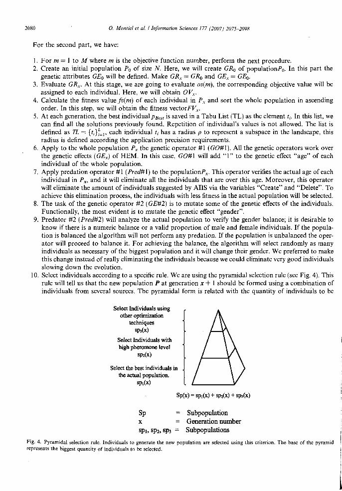
10. Select individuals according to a specific rule. We are using the pyramidal selection rule (see Fig. 4). This rule wilI telI us that the new population P at generation x + 1 should be formed using a combination of individuals from several sources. The pyramidal form is related with the quantity of individuals to be

Select Individuals using other optimization

techniques SP3(X)

Select Individuals with high pheromone level

sP2(x)

Select the best individuals in tbe actual population.

sp¡(x)

Sp(x) = sp¡(x) + SP2(x) + Sp3(X)

Subpopulation Generation number Subpopulations

Fig. 4. Pyramidal selection rule. lndividuals to generate the new population are selected using this criterion. The base of the pyramid represents the biggest quantity of individuals to be selected.

2081 o. Montiel e/ al. I Informa/ion Sciences 177 (2007) 2075-2098

selected; for example, the base is the biggest part of the pyramid and it is representing the biggest quan­tity of determined class of individuals to be selected, in this case a percentage of the best individuals of the actual populationp¡(x). In the next level, at the middle, we have a percentage ofindividuals with high pheromone level P2(X). At the top, we have individuals selected from other optimization methods P3(X). In this way, we are allowing a natural hybrid functionality.

11. Utilize the genetic operator #3 (GO#3) to increase the pheromone level of the best individuals (base of pyramid) that were selected in step lO.

12. Create a new population of size actPs (actual population size) using the subpopulation formed by the selected individuals at step 10. a. Parent selection is made according to what was programmed in the genetic effect "gender". If we

selected to use a population ofmale and female individuals, then we have to select randomly one indi­vidual of each classification to perform the recombination. On the other hand, if we are not consid­ering the gender, then we have to select two individuals from the same population. We used the Extended intermediate recombination operator given by Eq. (3) [22,24]. One strategy that gives good results is to achieve the parent's selection with a probability of 80% of being of different sex (class), the rest can be of the same sex, and even we can select the same individual twice. Randomly, create and assign the genetic effects to the new individual.

b. Apply the mutation operator to the genetic representation (gr) of the new individual. We are using the mutation operator defined by Eq. (4).

c. Apply Predator #3 (Pred#3) to the recentIy created individual. This operator is dedicated to eliminate all the individuals that are out of the valid search space. This operator can be programmed in two ways: One is to eliminate individuals, which parametric values gr went out the search space; this is a drastic solution because we can eliminate individuals that are very near to the optimum. A better solution is to adjust (correct) the decision variables that are out of range in such a way that the cor­responding values fall in the nearest boundary.

d. Calculate the objective values of the new individual. 13. Considering the best individual of the last generations (we used the last 10 generations), calculate the

variance value of these individuals using their fitness value. We are using the variable "Variance" to store this value.

14. We are using the variable "Cycling" to indicate the number of generations that the evolution has not had any significant change. We are measuring this change using the variable "Variance", if the obtained var­iance value is less than 0.05 in the last generations (10 generations), then increase the value of the var­iable "Cycling", otherwise reset its value.

15. Using AIIS calculate the amount of individuals that we have to eliminate, as well as the amount of indi­viduals that we have to create.

16. If AIIS determined that it is necessary to create more individuals, then we have two ways to create them. AIIS will determine the best option. a. Randomly, create a quantity of new individuals, this quantity is calculated by AIIS. This option

is very fast and the best option at the first stages because in average is very likely that the new generated individuals do not repeat the same search subspace, i.e. they do not fall in a previously visited point.

b. Create an individual out of the tabu regions, i.e., an individual that has not been included in the Tabu List TL and/or in the Visited Region List (VRL). Note that always at the first time VRL is empty, and it is filled with individual that has been selected as valid individual to complete the population size inferred by AIIS, this is to avoid repeating the selection of the same regions; i.e., individuals that pre­viously were created and selected. The VRL uses the same value of p that was used in step 5 for TL. The VRL is a complementary list of TL, and the use of both is very important since they allow the algorithm to perform an exhaustive search in the whole landscape.

17. Repeat steps 4-17, until we fulfill the termination criterion. 18. Save the decision variables for the current objective function, as well as the corresponding OVo

19. End for. (Of step 1).

2082 o. Montiel el al. / lnformalion Sciences 177 (2007) 2075-2098

20. Continue with the next objective, i.e. m = m + 1; otherwise proceed with step 21. 21. End.

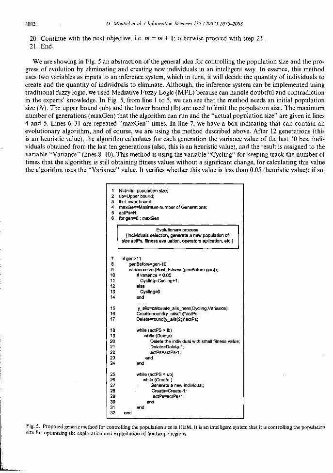
We are showing in Fig. 5 an abstraction of the general idea for controlling the population size and the pro­gress of evolution by eliminating and creating new individuals in an intelligent way. In essence, this method uses two variables as inputs to an inference system, which in turn, it will decide the quantity of individuals to create and the quantity of individuals to eliminate. Although, the inference system can be implemented using traditional fuzzy logic, we used Mediative Fuzzy Logic (MFL) because can handle doubtful and contradiction in the experts' knowledge. In Fig. 5, from line 1 to 5, we can see that the method needs an initial population size (N). The upper bound (ub) and the lower bound (lb) are used to limit the population size. The maximum number of generations (maxGen) that the algorithm can run and the "actual population size" are given in lines 4 and 5. Lines 6-31 are repeated "maxGen" times. In line 7, we have a box indicating that can contain an evolutionary algorithm, and of course, we are using the method described aboye. After 12 generations (this is an heuristic value), the algorithm calculates for each generation the variance value of the last 10 best indi­viduals obtained from the last ten generations (also, this is an heuristic value), and the result is assigned to the variable "Variance" (lines 8-10). This method is using the variable "Cycling" for keeping track the number of times that the algorithm is still obtaining fitness values without a significant change, for calculating this value the algorithm uses the "Variance" value. It verifies whether this value is less than 0.05 (heuristic value); if so,

1 N=lnitial populalion size; 2 ub=Upper bound; 3 Ib=Lower bound; 4 maxGen=Maximum number of Generalions; 5 acIPs=N; 6 for gen=O : maxGen

Evolutionary process (Individuals seleclion, generale a new population of

size actPs, filness evalualion, operators aplication, etc.)

7 if gen>11 8 genBefore=gen-10; 9 variance=var(Best_Fitness(genBefore:gen)); 1O If variance < 0.05 11 Cycling=Cycling+1; 12 else 13 Cycling=O 14 end

15 Laiis=calculate_aiis_hem(Cycling,Variance); 16 Create=round(Laiis(1 ))*actPs; 17 Delele=round(Laiis(2))*actPs;

18 while (actPS > lb) 19 while (Delele) 20 Delete the individual wilh small fitness value; 21 Delete=Delete-1; 22 actPs=actPs-1; 23 end 24 end

25 while (actPS < ub) 26 while (Creale ) 27 Generele a new individual; 28 Creale=Create-1; 29 actPs=actPs+1 : 30 end 31 end 32 end

Fig. S. Proposed generic method for controlling the population size in HEM. lt is an intelligent system that it is controlling the population size for optimizing the exploration and exploitation of landscape regions.

2083 o. Montiel et al. I Information Sciences 177 (2007) 2075-2098

then the variable "Cycling" is incremented (line 12), otherwise the variable is reset (line 14). The MFL infer­ence system will calculate the quantity of individuals that should be created and deleted, the result is assigned to the variable "y-aiis" (line 16); using this value, in line 17 the algorithm obtains an integer value of individ­uals to create, the result is assigned to the variable "Create". Similarly, in line 18 the quantity of individuals that have to be deleted are calculated, and the resuIting value is assigned to the variable "Delete". Lines 19-25 are dedicated to delete the quantity of individuals contained in the variable Delete. This elimination is made provided the actual population size stil1 being greater than the lower bound value (lb). Using line 21 the worst individual in the population is eliminated, line 22 updates de quantity of individuals to be eliminated, and in line 23 the actual population size (variable "actPs") is updated. Lines 26-32 are used in the process of creating new individuals, the quantity is indicated in the variable "Create". The algorithm will create new individuals as long as the actual population size does not exceed the upper bound (ub). A new individual can be created at random, using a tabu like method, and/or using a combination of both methods. After that, the variables "Create" and "actPS" are updated. Note that new population is stil1 being created in line 7, in other words, the evolutionary process creates the new population using the common procedures for selection, recombina­tion and mutation. The difference stems in that this method exploits determined region with the less individuals as can be possible, for speeding up the process; of course, diversity is lost but we do not take care for it, because HEM is able to advance the evolution when the algorithm has exploited exhaustively the region, i.e., we cannot get better fitness values.

2.2. Genetic operators to modify the genetic representation

2.2.1. Recombination operator We are using the Extended Intermediate Recombination (EIR) operator. To use this operator, we are

considering that we selected two parents X = (x ..... ,xn) and Y = (YI,'" ,Yn) to obtain the successor Z = (z ... .. ,zn)' Classical1y, for this operator the parents are selected such that X #- Y. Because, the process of test­ing this last condition takes time, we obtained an 80% of individuals using the original approach, we separated the individuals in two c1asses, male and females, and we selected one individual of each class to achieve the recombination. For the remaining 20%, we al10wed to mating individuals of the same class. The EIR operator is given by Eq. (3)

Z¡=X¡+IX¡(y¡-X¡), i= l, ... ,n (3)

where lXi E [-d, 1 + d] is chosen with uniform probability for each i, and d ~ O, a good choice is d = 0.25, which is the one that was used.

2.2.2. Mutation operator The goal of the mutation operator is to modify one or more parameters of Z¡, the modified objects (i.e., the

offsprings) that appear in the landscape within a certain distance ofthe unmodified objects (i.e. the parents). In this way, a coefficient z' of the offspring Z, is given by

z' = Z¡ ± range¡ . 15

where rangei defines the mutation range, and it is calculated as

range¡ = A . searchinterval¡

(4)

(5)

In the Discrete Mutation operator (DM), A is normally set to 0.1 or 0.2 and it is very efficient with sorne func­tions, but also we can set it to l. This is the case of the Broad Mutation Operator (BM) proposed in [29] to solve problems where the distance between the optimum and the actual position is 1arger than the DM oper­ator could reach. We wil1 have in one step, that the mutation operator can reach points from =¡ only within the distance given by ±rangei' 15. The sign + or - is chosen with probability of 0.5. The variable 15 is computed by

K-I

15 = ¿Ip¡r', lpiE{O,I} (6) ¡=O

iI

2084 o. Montiel et al. / Information Sciences 177 (2007) 2075-2098

Before mutation is applied, we set each ({Ji equal to 0, and then each ({Ji is mutated to I with probability Pb = k, and only ({Ji = I contributes to the sumo On the average there will be just one ({Ji with value 1, say 'Pi; this is done for each coefficient, in this way several coefficients of the same vector might be mutated. Then b is given by [7,23J

b = r i (7) In formula (6), K is a parameter original1y related to the machine precision, i.e. the number of bits used to represent a real variable in the machine that we are working with, traditionally K uses values of 8 and 16. In practice, however, the value of K is related to the expected number of mutation steps, in other words, the higher the value of K is, the more fine-grained is the resultant mutation operator [2].

2.3. Mediative fuzzy logic

MFL is a novel method for performing inference in presence of doubtful and contradictory information [20,21]. MFL was proposed as an extension of traditional fuzzy logic and includes Intuitionistic fuzzy Logic (IFL) in the Atanassov sense [1,4,15,33].

A set e in MFL is given by

e = {(x, .udx) , vc(x)) Ix E X} (8) where .uc: X --+ [0, lJ and Vc: X --+ [0, lJ are the agreement and non-agreement membership functions.

In the same way as in intuitionistic fuzzy logic in the Atanassov sense, for a fuzzy set e we have a "hesi­tation margin" nc(x) defined by equation

nc(x) = 1 - .udx) - vdx) (9)

where

(10)

and .uc(x); vc(x) E [0, lJ denotes a degree of membership and a degree of non-membership of x E e, respec­tively [3].

A contradiction fuzzy set e in X is given by

(dx) = min(.udx), vc(x)) (11 )

we can say that for each x E X we have a "contradiction index" value (c that indicates the degree of contra­diction in the knowledge for the x value. For calculating the inference at the system's output, we are using

MFS= (l-n-DFS1, + (n+DFSv (12)

where FSI' is the inference at the output using only the agreement membership functions, and FSv is the output using only the non-agreement membership functions.

2.4. The artificial intel/igent intuitive system

The control ofpopulation size is achieved via theAIIS and it is feedback method based in MFL. We preferred to use MFL in the inference system because can handle the knowledge in a more robust way since MFL can make inferences taking into account doubtful and contradictory knowledge. Moreover, if there is no contradiction or doubtful, the MFL system auto-reduces itself to behave as a traditional or intuitionistic fuzzy logic system.

Basical1y, at present time, the MFL method in HEM uses two variables. The variable "Variance" to control the variance value, and the variable "Cyc1ing" to control the number of generations that the population remains in the same landscape region arid/or without any significative change in the variance measurement. For the first one, we use the fitness value of the best individual of previous generations (we used 10 genera­tions), to calculate their variance. For measuring the degree of cyc1ing, at each generation we calculate th~ variable "Variance" and we make an increment in the variable "Cycling" each time the variable "Variance" is below a predetermined threshold value, we fixed this value to 0.05; otherwise reset the variable "Cycling", i.e. "Cycling = O". The threshold value was obtained experimental1y, testing several complex test functions.

I [ I

11

j

2085 O. Montiel el al. / Informalion Sciences 177 (2007) 2075-2098

The inteJligent system will calculate the quantity of individuals that should be eliminated from the actual pop­ulation, as well as the individuals that should be created in the actual population. We have two choices for creating individuals, the first one is to create individuals randomly, the second way is to use a Tabu search method for avoiding the tabu regions and create the new individual out these regions. Always, the operation of deletion is performed first, then we proceed to create the new individuals.

We used two Sugeno inference systems of order O, one for the agre~ment side, and the other one for the non­agreement side. In Table 1, we are summarizing the linguistic variables that we used in the fuzzy system: Each inference system has two output variables named "Delete" and "Create". The values of these two variables are related to the amount of individuals that should be eliminated or created. Each output variable has three con­stant terms, which are: "Iittle", "regular", and "many". We assigned the values of "O", "0.5", and "1", respec­tively. We used the same name and values at the output ofeach inference system (agreement and non-agreement).

At the agreement side we have the following 16 rules:

1. If (Cyc!ing is SmallC) and (Variance is SmallV) then (Create is little)(Delete is little) 2. If (Cyc1ing is SmallC) and (Variance is RegularV) then (Create is regular)(Delete is little) 3. If (Cyc1ing is SmallC) and (Variance is LargeV) then (Create is regular)(Delete is regular) 4. If (Cyc1ing is RegularC) and (Variance is SmallV) then (Create is many)(Delete is regular) 5. If (Cyc1ing is RegularC) and (Variance is RegularV) then (Create is regular)(Delete is regular) 6. If (Cyc1ing is RegularC) and (Variance is LargeV) then (Create is regular)(Delete is regular) 7. If (Cyc!ing is LargeC) and (Variance is SmallV) then (Create is many)(Delete is many) 8. If (Cyc1ing is LargeC) and (Variance is RegularV) then (Create is many)(Delete is regular) 9. If (Cyc1ing is LargeC) and (Variance is LargeV) then (Create is little)(Delete is little)

lO. If (Cyc1ing is SmallC) and (Variance is XLargeV) then (Create is little)(Delete is regular) 11. If (Cyc1ing is RegularC) and (Variance is XLargeV) then (Create is regular)(Delete is little) 12. If (Cyc1ing is LargeC) and (Variance is XLargeV) then (Create is little)(Delete is little) 13. If (Cyc1ing is XLargeC) and (Variance is SmallV) then (Create is many)(Delete is many) 14. If (Cyc!ing is XLargeC) and (Variance is RegularV) then (Create is many)(Delete is many) 15. If (Cyc!ing is XLargeC) and (Variance is XLargeV) then (Create is many)(Delete is many) 16. If (Cyc1ing is XLargeC) and (Variance is LargeV) then (Create is many)(Delete is many)

At the non-agreement side we have the following four rules:

1. If (Cyc1ing is nLargeC) and (Variance is nLargeV) then (Create is little)(Delete is little) 2. If (Cyc1ing is nLargeC) and (Variance is nSmallV) then (Create is little)(Delete is little) 3. If (Cyc1ing is nSmallC) and (Variance is nLargeV) then (Create is many)(Delete is many) 4. If (Cyc1ing is nSmallC) and (Variance is nSmallV) then (Create is regular)(Delete is regular)

Table 1 Name, type, and parameters of the linguistic variables for each Fuzzy Inference System (FIS)

FIS name Variable name Term name Type Parameters

AlISa (FS,,) Cycling SmallC Trapezoidal [-1, -1,5,30] AlISa (FS¡,) Cycling RegularC Triangular [10,30,50] AlISa (FS,,) Cycling LargeC Triangular [30,50,70] AlISa (FS,.J Cycling XLargeC Trapezoidal [50,70, 5e+ 15, 5e+ 15] AlISa (FS,,) Variance SmallV Trapezoidal [-1, -1, 0.04, 0.2] AlISa (FS,,) Variance RegularV Triangular [0,0.2,0.4] AlISa (FS~) Variance LargeV Triangular [0.2,0.4,0.6] AlISa (FS,,) Variance XlargeV Trapezoidal [0.4,0.6, 5e+ 15, 5e+15] AIISna (FS,.) Cycling nLargeC Trapezoidal [-1, -1, 10,60] AIISna (FS,.) Cycling nSmallC Trapezoidal [1O,60,5e+15,5e+15] AIISna (FS,.) Variance nLargeV Trapezoidal [-1, -1,0.05, \] AIISna (FS,.) Variance nSmallV Trapezoidal [-1,0.09, \, 5e+ 15]

In the agreement side, we are identifying the agreement side using (AlISa), and the non-agreement side with AIISna .

2086 o. Montiel et al. I Information Sciences 177 (2007) 2075-2098

The agreement and non-agreement membership function were established by two different experts. At the agreement side, for example, considering rule 1, we have that for smal1 values of the variables

"Cycling" and "Variance" it is necessary to "Delete" a "Iittle" quantity of individuals and then "Create" a "Iittie" quantity of individuals. In other words, if AIlS has begin to detect that the algorithm in the last gen­erations has not had a significative increment in the fitness value of the best individuals then is necessary to "Delete" a smal1 quantity of individuals (the less fit individuals), then "Create" a smal1 quantity of individuals to increase the explorative skills of the algorithm. If "Variance" remains being "Smal1" the value of the var­iable "Cycling" is increased (rule 4 at the agreement side) and the algorithm should "Delete" more individuals (a regular quantity) and "Create" many individuals, and so on.

2.5. Generating the new population

HEM has three ways to generate new individuals, they are:

l. The basic method is to use a subpopulation of individuals that were selected with the pyramidal rule (step 10 of HEM), then the new individuals are obtained applying the recombination and mutation operators (steps 12a and 12b of HEM), this part is very similar to others EAs; the difference is the use ofthe operator Pred#3 that basical1y is repairing individuals with decision variables out of a valid range (step 12c of HEM).

2. AIIS can determine wheter is necessary to create new individuals using random search (step 16a). The quan­tity of new individuals is variable and depends on the degree of cycling that the algorithm is having. More­over, AIIS determines the quantity of individuals in the actual population that we have to eliminate, AIIS wil1 select the less fit individuals in the population to eliminate them. The new population will be formed by a combination of individuals generated using steps 1 and 2 of this Section 2.5; also, a possibility is that new populations wil1 be formed only by individuals randomly generated.

3. The third way is more complex and time consuming but it is very efficient when we could not advance in evolution using steps I and 2 of this section. Similarly than in step 2, AIIS wil1 determine the amount of individuals to create and eliminate, but the new individuals will be created using tabu regions for avoiding create a successor in this region. HEM basical1y is using a Tabu List (TL) where the best solutions at each generation is saved, and a Visited Region List where HEM is saving the already visited regions in the pro­cess of creating new successors [14]. The TL is defined as TL = {ti}~=\' in this list we are saving the whole individual Pll' VRL is defined by VRL = {((i, Pi' lpi)):' where Vis the number of al1 visited regions; (i is the center of a visited region which is a sphere with radios Pi; and the frequency of visiting this region is rep­resented by lpi. Step 2 is faster than step 3, and it is an option for going out traps.

3. Benchmark functions description

As it was mentioned in the introduction, several classical benchmark functions as wel1 as a novel composite test functions suite special1y designed for testing optimization algorithms were used. Next, we are giving a brief description of them.

3.1. Classical test functions

The Sphere function (FI) is quadratic, continuous, convex, and unimodal. For D dimensions the minimum is Oat the origin; i.e. x· = [0"02",, ,OD). This function provides an easily analyzable first test for the optimi­zation algorithm.

The Rosenbrock function (F2) is quadratic, continuous, non-convex, unimodal. For D dimensions, this function has its global minima at x· = [l lo 12" .. , ID). This function is considered as a nightmare for most of the optimization algorithms because it has deep parabolic valley along the curve XH 1 = x1. AIgorithms that are not able to discover good directions underperform in this problem.

The Step function (F3) is discontinuous, non-convex, and unimodal. This function is used as a representa­tion of problems with flat surfaces that are considered as obstacles for optimization algorithms, because they

2087 o. Montiel et al. I Information Sciences 177 (2007) 2075-2098

do not give any information about which is the feasible direction. The main idea of this function is to make the search more difficult by introducing small plateaus to the topology. Using the range [-5.12,5.12], the mini­mum of this function for two dimensions is -10; similarly, for four dimensions the minimum is -20.

The Quartic function (F4) is quadratic, continuous, convex, unimodal padded with Gaussian noise. The fact of introducing noise to the function causes that the algorithm never gets the same value on the same point. Algorithms that do not work well optimizing this function will work poorly on surfaces with noisy data.

The Foxholes function (F5) is continuous, non-convex, non-quadratic, two-dimensional with 25 local min­ima located approximately at the point {(alj, a2j)}~:" and the value at the points (alj, a2j) is approximatelycj. De long in his work defined the next values for aij,

[ -32

[aij] = -32 -16

-32

O

-32

16

-32

32

-32

-32

-16

-16

-16

O

32

16

32 32] 32

(13)

where Cj = j and K = 500.

rabie 2 De Jong's test suite (FI-F5), Rastringin function

Name Function Limits

Sphere function FI

Rosenbrock function F2

Step function F3

Quartic function F4

Foxholes F5

Rastrigin F6

Weierstrass's function

Griewank's function

Ackley's function

N

FI(X) = ¿x¡ ;=1

N-I

F2(X) = ¿(lOO * (X;+I _ '¿')2 + (Xi _ 1)2) ;=1

N

F3(X) = ¿lx;J ;=1

N-I

F4(X) = ¿i ·x4 + GAUSS(O, 1) ;=1

1 1 25 1-=-+¿­F5(X) K j=1 Jj(X)

where ,

¡; = Cj + !)x; - aij)6

;=1

" F6(X) = A . n + ¿ x¡ - A . cos(W . Xi)

;=1

o , o ()f(x) = {; 4~~0 - TI cos ~ + 1

f(x) = -20exp (-0.2 ~ tx¡)-exp (~t COS(2lUi)) + 20 + e

-IO<x;< 10

-2.048 < Xi < 2.048

-5.12<xi<5.12

-1.28 < Xi < 1.28

-65.536 < Xi < 65.536

-10 < Xi < 10

a =0.5, b = 3, kmax = 20, X E [-0.5, 0.5t

X E [-100,100t

X E [-32,32]D

For aH the functions N is the number of dimensions, in F3, lXiJ represents the greatest integer less than or equal to Xi; in F6, A is the amplitude and IV the frequency. We tested functions FI and F6 using a range of[-IO, lO).

2088 o. Montiel et al. / ln{ormation Sciences 177 (2007) 2075-2098

Rastrigin's function (F6) is continuous, non-convex, and multimodal. It is a fairly difficult problem for evo­lutionary algorithms due to the large search space and large number of local minima. The surface of the func­tion is determined by the variables A and w, which control the amplitude and frequency of the modulation, respectively. The global minima is located at x· = [Ob02," .,ODJ.

3.2. Composite test Junctions

The basic set of composite test functions are composed by 10 basic functions (jI-lO = JI ... JIO) for lO-D (Dimensions), the search range for aH the functions is [-S, st. The basic set is given by the Sphere, Rastrigin, Weierstrass, Griewank, and Acley's functions, see Table 2 for the specific formulas. In [16] a method is given for constructing these Composite Functions.

......

...,.-'

. .

-"'"

...,. -......­ ...­ o

......

200· .

800­

400 ­ .

800·­ ..

1000·­ ..

1200,- .

1400­

-5 ':l

Fig. 6. 2-D Composite Function 1 (CF 1j.

Fig. 7. 2-D Composite Function 2 (CF2).

5

I I

1

2089 o. Montid et al. I Information Sciences 177 (2007) 2075-2098

In general we have that the multimodal Composite Function CFl (Fig. 6) was constructed using 10 unimo­dal sphere functions ({1~1O)' this resulting function has one global optimum and nine local optima.

CF2 (Fig. 7), and CF3 (Fig. 8) were constructed using 10 Griewank's and Rastrigin's functions ({l-IO), respectively. Because they have more complex multimodal functions, localizing their local optima becomes more complexo For this function the global optimum is very difficult to reach even when the global optimum area has been found.

CF4, CF5, and CF6 are all called hybrid functions because they were constructed with different basic functions.

To construct CF4 (Fig. 9) we have:f¡_2(X): Acley's function,/J-4(x): Rastrigin's function,fs_6(x): Weierst­rass function, h~8(X): Griewank's function, h-lO(X): Sphere function.

...... . ....

.....

3500" ..... .... .....

3000" .. "

2500·

2000....

!lOO" ..., ..

o 5

. ....

. ,

......

.­ -....-.

Fig. 8. 2-D Composite Function 3 (CF3).

5 , .•...­....--

Fig. 9. 2-D Composite Function 4 (CF4).

2090 O. Montiel e/ al. / Informa/ion Sciences 177 (2007) 2075-2098

Fig. 10. 2-D Composite Function 5 (CF5).

2000

1000.

500.

O. 6'- '.

\'.

\

.. ",- ----.:- -"'.~ -~ ...;----~._,----

.2 ·3--- ...\---- ....~ -- o ~1

2

Fig. 11. 2-D Composite Function 6 (CF6).

CF5 (Fig. la) is composed by the functions: fl-2(X): Rastrigin's function, !,-4(X): Weierstrass function, fS-6(X): Griewank's function, f7-S(X): Ac1ey's function, f9-IO(X): Sphere function.

CF6 (Fig. 11) is composed by the functions: fl-2(X): Rastrigin's function, f3-4(X): Weierstrass function, fs-6Cx): Griewank's function, f7 s(x): Ac1ey's function, f9-IO(X): Sphere function.

The construction of composite functions requires a methodo1ogy, like the one given in [16J.

4. Experimental results

Several experiments were performed, and they were c1assified in two groups: experiments with c1assical test functions, and experiments with composite test functions.

2091 o. Montiel et al. IInformation Sciences 177 (2007) 2075-2098

For aH the tests the HEM model was used, as was described in Section 2. The HEM model was not allowed to work in hybrid mode because the idea is to test the functionality of the method without the intervention of any other algorithm. New individuals were created using the procedures explained in Section 2.5 (sections l and 2). For achieving the recombination process, we selected a percentage of the best individuals (20%), and a percentage of individuals with highest pherhomone level (2%) (value of the genetic effect ge(phLevel) of each individual). Others specific HEM's parameters are given in the corresponding tests in Tables 4-6.

All the tests were done in a Pentium 4 computer (DELL Optiplex GX620j with Windows XP platform. All the programs were tested in Matlab programming language version 7.1.

4. J. Group J. Experiments with classical test functions

We performed experiments using the De Jong's test function suite, as well as the Rastrigin function. In Table 2 we show the formula for each function (FI to F6). We compared our results against the results obtained using a Genetic AIgorithm (GA). We decided to use the Genetic AIgorithm of Matlab's Toolbox to perform the comparison because it provides an easy way to reproduce the results presented in this work. In Table 3 are the selected options for the Matlab's GA.

We made comparisons of processing time and average precision for each test function and for each method. Each test was conducted in the next form:

a. For each test function (FI to F6), we selected the most suitable parameters for the GA for achieving a good statistical result for 100 mns for the corresponding function.

b. We executed the GA lOO times and we saved the best fitness value (maximal fitness), the minimum fitness value, and the statistical values of mean, median and standard deviation achieved in the 100 mns.

c. We chose the parameters of HEM in such a way to obtain a notable difference in precision in favor of HEM. We used statistical t-Student test to ensure that statistical processes are different. In the same way than in step c, we saved the results of the lOO tests.

d. We compare the average time of both algorithms, and we obtained the statistical to value [19].

Steps "a" to "d" were done for two and eight variables (2 and 8 dimensions). In Tables 4 and 5, we are showing a comparison between the results obtained using HEM and the GA of Matlab for the six abovemen­tioned test functions Fl to F6. In Table 4 we used two decision variables, and eight variables for Table 5. In all of the cases, we executed each algorithm 100 times for obtaining statistical meaningful results. In these

Table 3 We used these options in the GA Toolbox of Matlab for testing the Test Suite of Table 2

Options

PopulationType 'doubleVector' InitialPopulation [] PopInitRange [2 x 1 double] InitialScores [ ] PopulationSize SO InitialPena1ty 10 EliteCount 2 Pena1tyFactor 100 CrossoverFraction 0.8000 PlotInterval 1 MigrationDirection 'forward' CreationFcn @gacreationuniform MigrationInterval 20 FitnessScalingFcn @fitscalingrank MigrationFraction 0.2000 SelectionFcn @selectionstochunif Generations 80 CrossoverFcn @crossoverscattered TimeLimit Inf MutationFcn @mutationgaussian FitnessLimit -Inf HybridFcn [] StallGenLimit 80 Display 'final' StallTimeLimit 20 PlotFcns [] TolFun l.OOOOe-006 OutputFcns [] TolCon 1.0000e-006 Vectorized 'off

2092 o. Montiel et a/. / Information Sciences 177 (2007) 2075-2098

Table 4 Two dimensions

FI F2 F3 F4 F5 F6

HEM GA HEM GA HEM GA HEM GA HEM GA HEM GA

Generations Age Ni Nub Nlb Maximum fitness Minimum fitness Mean value Median Standard deviation Average time (s)

30 4 lO 600 lO 4.20e9 133.35 I.I1e8 3.14e5 5.7ge8 0.131

lOO

20

7.5e4 15.63 1.66e3 255.01 7.78e3 0.145

60 4 300 1000 lO 5.25e10 121.38 5.44e8 1.24e5 5.25e9 0.92

200

lOO

l.72e6 145.83 3.1ge4 2.28e3 l.78e5 0.98

40 4 20 50 10 -10 -10 -lO -10 O 0.26

500

300

-6 8 0.65 -5 6.25 0.52

30 4 10 600 10 116.71 1.01 7.58 2.29 17.30 0.135

500

300

85.28 1.00 5.87 2.30 10.90 6.647

50 4 10 100 20 1.002 1.002 1.002 1.002 2.5ge-11 0.866

200

40

1.002 1.0007 1.0020 1.002 1.7ge-4 1.211

40 4 lO 600 10 I.31e9 122.9 1.8ge7 4.60e5 I.31e8 0.206

200

lOO

6.le3 5.4 580.17 110.17 1.I5e3 0.871

Time difference (s) Statistic t-test (lo)

0.0138 -1.9240

0.06 -1.0359

0.26 17.0348

6.512 -1.924

0.345 O

0.665 -1.4447

We show results of the optimization of the De Jong's test suit (FI-F5), and the Rastrigin function for two decision variables. We use as optimization methods, the HEM and the GA from the Matlab's toolbox. In the first column we are showing the variables values that we use for both evolutionary algorithms; note that the GA does not require sorne of them because they are specific for HEM.

Table 5 Eight dimensions

FI F2 F3 F4 F6

HEM GA HEM GA HEM GA HEM GA HEM GA

Generations 60 250 5000 5200 100 5000 2000 1000 130 800 Age 8 10 8 8 16 Ni 50 50 200 800 20 1000 100 500 50 300 Nub 600 250 200 800 600 Nlb 10 100 10 20 10 Maximum fitness 3.64e4 193.41 21.72 13.91 -40 -34 295.13 41.51 9.31e5 81.80 Minimum fitness 47.65 13.13 0.9230 0.9015 -36 -22.5 0.9994 0.9962 557.90 2.20 Mean value 3.78e3 45.92 13.62 0.9015 -39.41 -20.5 6.4239 4.6885 5.92e4 13.50 Median 1.24e3 34.84 13.57 0.5707 -40 -20.5 2.2034 2.1450 1.6ge4 9.69 Standard deviation 6.80e3 33.20 3.39 1.54 1.0833 6.45 29.69 7.3404 1.26e5 12.40 Average time (s) 0.4481 0.5970 263.74 286.85 1.1359 0.658 20.70 24.465 2.561 3.53

Time difference (s) 0.1489 23.11 t (The GA found 3.7650 0.9692 values very far the

optimal value) Statistic t-test (lo) -5.4930 -34.15 60.34 -5.4930 -4.71

Optimization of the De Jong's test suite (FI-F4), and the Rastrigin function for eight decision variables. We use as optimization methods, the HEM and the GA from the Mat1ab's toolbox. In this case, we do not optimize F5 since it is defined for two dimensions. Here, t means that the comparison does not apply because the GA could not found the optimal value, or the value founded is far from the optimal.

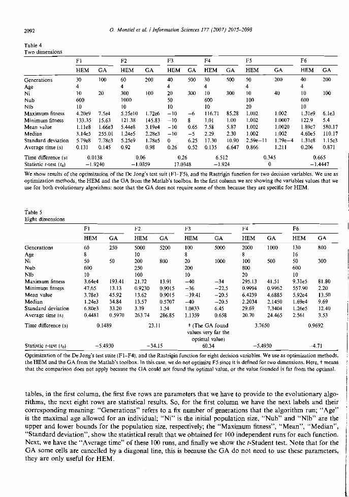
tables, in the first column, the first five rows are parameters that we have to provide to the evolutionary algo­rithms, the next eight rows are statistical results. So, for the first column we have the next labe1s and their corresponding meaning: "Generations" refers to a fix number of generations that the algorithm run; "Age" is the maximal age al10wed for an individual; "Ni" is the initial population size, "Nub" and "Nlb" are the ¡ upper and lower bounds for the population size, respectively; the "Maximum fitness", "Mean", "Median", I "Standard deviation", show the statistical result that we obtained for 100 independent runs for each function. I Next, we have the "Average time" ofthese 100 mns, and final1y we show the t-Student test. Note that for the GA sorne cells are cancel1ed by a diagonal line, this is because the GA do not need to use these parameters, they are only useful for REM. I

1

2093 o. Montiel et al. I Information Sciences 177 (2007) 2075-2098

In this group of tests for the recombination operator we used d = 0.25 to calculate ~ of Eq. (3); and for the mutation operator we used A= 0.1 in Eq. (5) for aH the cases, except for the Foxholes function where we used a value of 0.5 for this variable.

4.2. Group 2. Experiments with composite test functions

We considered as benchmark target values the results reported in [16] for the algorithms PSO, CPSO, CLPSO, CMA-ES, G3-PCX, and DE. In this work the best objective value reported for the composite test function is 5.7348 x 10-8

, so we used that va1ue as the stopping criteria for HEM in this group of tests, a

Table 6 10 dímensions Composite Functions optimization usíng HEM

CFI CF2 CF3 CF4 CF5 CF6

Generations 300 500 300 500 500 500 Age 20 20 25 20 20 20 Ni (initial population size) 600 1000 600 1000 1000 1000 Nub (population's upper bound) 600 1000 600 1000 1000 1000 Nlb (population's lower bound) 100 150 100 150 ISO 150 Mínimum objective value (best) 2.7Ie-8 5.7ge-8 5.46e-0 200 3.7882e-2 400.52 Maximum objective value 4.9ge-8 2.35 206.03 278.98 4.3903 500.74 Mean value 4.3ge-8 0.12 77.63 240.83 1.8190 495.08 Median 4.5ge-8 2.68e-6 72.83 252.43 1.4048 500.00 Standard deviation 6.400-9 0.53 69.78 24.44 1.3510 22.26 Average time (s) 196 2059 804 2828 2758 2942 Success relation 20/20 19/20 7/20 0/20 4/20 0/20 Average of population size 49 475 318 521 508 531

We obtained statistics results runníng 20 times HEM for each composite function.

Table 7 Comparative results

CFI CF2 CF3 CF4 CF5 CF6

HEM Mean 4.3ge-8 0.12 77.63 240.83 1.82 495.08 Std. 6.46e-9 0.53 69.78 24.44 1.35 22.26

PSO Mean 100.00 155.91 172.03 314.30 83.45 861.42 Std. 81.650 131.76 32.87 20.07 101.11 125.81

CPSO Mean 156.26 242.29 362.64 522.37 255.56 853.14 Std. 134.27 148.95 196.31 122.09 175.63 127.98

CLPSO Mean 5.74e-8 19.16 132.81 322.32 5.371 501.16 Std. 1.04e-7 14.75 20.03 27.46 2.61 0.78

CMA-ES Mean 100.00 161.99 214.06 616.40 3.585 900.26e Std. 188.58 151.00 74.18 671.92 168.26 0.083

G3-PCX Mean 60.000 92.699 319.80 492.96 26.02 772.08 Std. 69.93 99.07 125.19 142.49 41.58 189.39

DE Mean 0.07 28.76 144.41 324.86 10.79 490.94 Std. 0.11 8.63 19.40 14.75 2.60 39.64

HEM outperforms the results obtained with the others methods. The over aH best optimization result obtained with determined algorithm (row) for the correspondingcomposition functíon (column) is highlighted (bold) and underlined. In addition, we híghlighted the best result obtained with HEM for CFI and CF6 because they are as good like the obtained with CLPSO for CFI, and DE for CF6. We underlined the best results obtained with any other algorithm different of HEM. Note: Optimization results for PSO, CPSO, CLPSO, CMA-ES, G3­PCX, and DE were taken from [16] as benchmarks.

>

2094 o. Montiel et al. / lnformation Sciences 177 (2007) 2075-2098

second criteria was the number of generations. In Table 6, the first five rows are for the specific parameters values used in HEM to achieve each test. In the fol1owing six rows we col1ected information for 20 runs for each composite function CFl to CF6 for 10 dimensions (Figs. 6-11), this is for being consistent with the result of the tests reported in [16]. We included one row labeled as "Success relation" for indicating a rela­tion of successful test vs. number of runs. The last row is for annotating the average population size in 20 runs that each test required.

In Table 7, we are comparing the results obtained with HEM for the composite functions against the results reported in [16]. To achieve this comparison HEM's statistics from Table 6 was used.

In this group of tests for the recombination operator a value of d = 0.25 was used to calculate a of Eq. (3); and for the mutation operator A= 0.1 was used in Eq. (5) for aH the cases.

5. Discussion

In this section, a discussion of the performed experiments is presented. The discussion was divided in two groups: "Group 1" for classical test function, and "Group 2" for the composite test functions.

5.1. Group l. Classical test functions

We have that always HEM works better than the GA of the Matlab's Toolbox. The best times and preci­sion finding the minimizer for this group of functions were obtained using HEM.

In Tables 4 and 5, we can appreciate that the best fitness values and the lower processing times were achieved using HEM. We selected the parameters of HEM for obtaining a better statistical behavior than the one obtained using the GA, this with the aim of making' comparisons of time, we noted that always the processing time and precision of REM outperformed the results obtained using the GA of Matlab. We performed many tests using 8, 16 and 32 variables and always we obtained better results using REM. We noticed that the more difficult is the problem the better results were obtained using REM. The Foxholes func­tion (F5) is a difficult function that tests the explorative capacity of evolutionary algorithms, also in this test REM worked better, but we observed that in this case REM always needed a mutation step size ofO.5, instead of 0.1 like in the other cases.

We conducted additional tests for 16, 32 and 64 decision variables for testing functions Fl to F6 ofTable 2. For example, in Figs. 12 and 13, we show results of the optimization of a Sphere function with 64 decision

F1: Filness behavior tor lhe Sphere tunction. 64-025,-------.----------'---.-----------,

20

15

10

0'-----===-----'--------'--------­O

generations 50 100

Fig. 12. Typical fitness plot for the Sphere function with 64 decision variables when it is optimized using REM.

2095 o. Montiel el al. I Informalion Sciences 177 (2007) 2075-2098

F1. 64-D. Dynamic behavior 01 lhe populalion size 1000,-------~-----_'___',------___,

900

900

700

<Il'51 aoo c:

~500 ~ 8. 400

300

200

100

oL

.

--J..._-=:=::::=-_b~::=:=__ _=:::::::.....J_ o 50 100 150

generalions

Fig. 13. Typical dynamics of populalion size for the Sphere function wilh 64 decision variables. We used HEM for oblaining lhe minimizers.

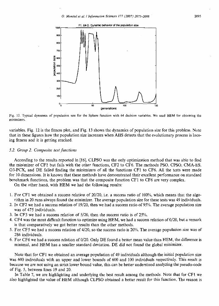
variables. Fig. 12 is the fitness plot, and Fig. 13 shows the dynamics of population size for this problem. Note that in these figures how the population size increases when AIIS detects that the evolutionary process is loos­ing fitness and it is getting stucked.

5.2. Group 2. Composite test functions

According to the resuits reported in [16], CLPSO was the only optimization method that was able to find the minimizer of CFl but fails with the other functions, CF2 to CF6. The methods PSO, CPSO, CMA-ES, G3-PCX, and DE failed finding the minimizers of aH the functions CFl to CF6. AH the tests were made for 10 dimensions. It is known that these methods have demonstrated their exceHent performance on standard benchmark functions, the problem was that the composite function CFI to CF6 are very complex.

On the other hand, with HEM we had the foHowing resuits:

1. For CFI we obtained a success relation of 20/20, i.e. a success ratio of 100%, which means that the algo­rithm in 20 mns always found the minimizer. The average population size for these tests was 49 individuals.

2. In CF2 we had a success relation of 19/20, then we had a success ratio of95%. The average population size was of 475 individuals.

3. In CF3 we had a success relation of 5/20, then the success ratio is of 25%. 4. CF4 was the most difficult function to optimize using HEM, we had a success relation ofO/20, but a remark

is that comparatively we got better resuits than the other methods. 5. For CF5 we had a success relation of 4/20, so the success ratio is 20%. The average population size was of

286 individuals. 6. For CF6 we had a success relation of 0/20. Only DE found a better mean value than HEM, the difference is

minimal, and HEM has a smaHer standard deviation. DE did not found the global minimizer.

Note that for CFl we obtained an average population of 49 individuals although the initial population size was 600 individuals with an upper and lower bounds of 600 and 100 individuals respectively. This result is because we are not using an strict lower bound value, this can be better understood analyzing the pseudo-code of Fig. 5, between lines 19 and 20.

In Table 7, we are highlighting and underiying the best resuit among the methods. Note that for CFl we also highlighted the value of HEM aithough CLPSO obtained a better result for this function. The reason is

2096 o. Montiel et al. I Information Sciences 177 (2007) 2075-2098

that HEM also found the minimizer with a very good approximation to zero, in this sense HEM works as well as CLPO finding the minimizer for the composite function CFl. In CF6 we highlighted the statistic values of CF6 because we considered that they are as good as those obtained with DE since differences are minimal.

We executed the algorithms 300 generations for CFl and CF3, and 500 generations for CF2, CF4, CF5, and CF6. HEM found solutions before the corresponding number of generations were achieved, for example for testing CF4, the best values were found around generation 50, so the time for finding this solution is more or less 200 seconds instead 1194 seconds. We have similar conditions in the other experiments. In Hg. 14 we are showing a typical fitness plot for the composite function CF2 for 10 decision variables, and in Fig. 15 we have its corresponding plot showing the dynamic behavior of population size for this test.

Fitness behavior

I 16

14

12

'" lO Q) '" c: e 8

6

r o!------'--~,,:::::::~===!~:=;::=~-----:-'_:______,'_::____::_:_~ o 50 100 150 200 250 300 350 400 450 500

generations

Fig. 14. Typical fitness plot for the composite function CF2 with 10 decision variables when it is optimized using HEM.

Dynamics 01 population siza 1000

l\900

BOO

700 <D N.0;

600c:

~ "3500

~ 400

300

200

100 O 50 100 150 200

~ 250 300 350 400 450

generations

I I i

1 I

500

Fig. 15. Typica1 dynamics of population size for the composite function CF2 with 10 decision variables when it is optimized using HEM.

2097 O. Mantie/ et al. / Infarmatian Sciences 177 (2007) 2075-2098

6. Conclusions

The use of composite test functions was very important since these functions are hard to optimize, we had to reconsider and make a general review of each step of HEM as previously proposed in [20], for example, we were considering one operator for c10ning the best individual in the population. This operator works great in our evolutionary model with c1assical test functions, but using the composite test function we realized that this operator was stucking the evolution.

HEM uses an intelligent strategy to "explore, exploit, ... , exploit, explore, ... ", so we can say that HEM always searches for a promissory region for being exploited. AIIS will maintain or increase the population size; once a convenient region is found, generally HEM reduces its population size with the purpose of speed­ing up the algorithm, this is done taking care of no diminishing the performance of the evolution; and when AIIS determines that this region has been exploited enough, then AIIS decides to increase the population size by generating new individuals randomly and/or using a tabu regions for avoiding falling in the same subspace, this is for being more explorative. In general, HEM has several mechanisms that work synergetically for per­forming search in an intelligent way. Hence, HEM is an intelligent evolutionary algorithm that uses knowl­edge from experts, and it is able to handle doubt and contradiction among human experts. An interesting thing that we observed is that almost always the dynamics of the population size for the same type of problem is behaves very similar.

In general, according the comparisons that we made, we can conc1ude that HEM outperformed the evolu­tionary algorithms PSO, CPSO, CLPSO, CMA-ES, G3-PCX and DE for the composite test functions CFI, CF2, CF3, CF5 and CF6.

We have demonstrated that having an intelligent evolutionary algorithm with the ability of learning from a group of experts is an interesting and promising idea. Future work may focus on improving the AIIS and increasing its knowledge data base with the aim of controlling more parameters of this evolutionary model.

Acknowledgements

The authors thank Comisión de Operación y Fomento de Actividades Académicas del I.P.N., and Instituto Tecnológico de Tijuana for supporting our research activities.

References

[1] K.T. Atanassov, Intuitionistic Fuzzy Sets: Theory and Applications, Springer-Verlag, Heidelberg, Germany, 1999. [2] L. Belanche, A study in function optimization with the breeder genetic algorithm, Research Report LSI-99-36-R. Universitad

Politécnica de Catalunya, 1999. Available from: <http://citeseer.nj.nec.com/belanche99study.html>. [3] O. Castillo, P. Melin, A new method for fuzzy inference, in: Intuitionistic Fuzzy Systems, Proceedings ofthe International Conference

NAFIPS 2003, IEEE Press, Chicago, Illinois, USA, 2003, pp. 20-25. [4] E. Co§kun, Systems on intuitionistic fuzzy special sets and intuitionistic fuzzy speciaJ measures, Information Sciences 128 (2000) 105­

118. [5] E.K.P. Chong, Stanislaw H. Zak, An Introduction to Optimization, second ed., Wiley, USA, 2001. [6] B.G.W. Craenen, A.E. Eiben, Computational Intelligence, online document consuited in 2006 May 28, Encyclopedia of Life Support

Sciences, EOLSS, EOLSS Co. LId. Available from: <http://www.xs4all.nl/-bcraenen/publications.html>. [7] 1. De Falco, A. Della Cioppa, P. Natale, E. Tarantino, Artificial neural networks optimization by means of evolutionary algorithms,

Soft Computing in Engineering Design and Manufacturing, Springer-Verlag, London, 1997. Available from: <http://cite­seer.ist.psu.edu/defalc097artificial.html> .

[8] K.A. De Jong, An analysis of the behaviour of a class of genetic adaptive systems, Ph.D. Thesis in Computer and Communication Science, University of Michigan, 1975.

[9] K. Deb, A. Anand, D. Joshi. A computationally efficient evolutionary algorithm for real-parameter optimization, KanGAL Report No. 20022003, 2002. Available from: <http://www.iitk.ac.in/kangal/reports.shtml#2002>.

[lO] K. Deb, Multi-Objective Optimization Using Evolutionary AIgorithms, John Wiley & Sons, LId., Great Bretain, 2002. [11] A.P. Engelbrecht, Fundamentals of Computational Swarm Intelligence, John Wiley & Sons, USA, 2006. [12] G.S. Ficici, Solution concepts in coevolutionary algorithms, Ph.D. Dissertation, Brandeis University, Computer Science Department

Technical Report CS-03-243, 2004. [13] N. Hansen, S.D. Muller, P. Koumoutaskos, Reducing the time complexity of the derandomized evolution strategy with covariance

matrix adaptation (CMA-ES), Evolutionary Computation II (2003) 1-18.

2098 o. Mantid el al. Ilnformalion Scíences 177 (2007) 2075-2098

[14] A.-R. Hedar, M. Fukushima, Tabu Search directed by direct search methods for nonlinear global optimization, European Journal of Operational Research 170 (2) (2006) 329-349.

[15] W.-L. Hung, J.-W. Wu, Correlation ofintuitionistic fuzzy sets by centroid method, Information Sciences 144 (2002) 219-225. [16] J.J. Liang, P.N. Suganthan, K. Deb, Novel composition test functions for numerical global optimization, in: IEEE Swarm Intelligence

Symposium, Pasadena California, USA, 2005, pp. 68-75. [17] J.1. Liang, A.K. Qin, P.N. Suganthan, S. Baskar, Evaluation ofcomprehensive learning particle swarm optimizer, Lecture Notes in

Computer Science 3316 (2004) 230-235. [18] L. Ljung, System Identification. Theory for the User, second ed., Prentice-Hall PTR, USA, 1999. [19] D.e. Montgomery, Design and Analysis of Experiments, fifth ed., John Wiley & Sons, Inc., USA, 2001. [20] O. Montiel, O. Castillo, P. Melin, R. Sepúlveda, Reducing the cycling problem in evolutionary algorithm, in: The 2005 International

Conference on Artificial Intelligence (lC-Ar05), Las Vegas Nevada, USA, 2005, pp. 426-432. [21] O. Montiel, O. Castillo, P. Melin, R. Sepúlveda, Mediative fuzzy logic: a novel approach for handling contradictory knowledge, in:

Proceedings of International Conference on Fuzzy Systems, Neural Neiworks and Genetic Algorithms, FNG 2005, Tijuana, BC, México, 2005.

[22] H. Mühlenbein, Evolutionary Algorithms: Theory and Applications. Available from: <http://citeseer.ist.psu.edu/110687.html>. [23] H. Mühlenbein, D. Schilierkamp-Voosen, Predictive model for breeder genetic algorithm: continuous parameter optimization,

Evolutionary Computation I (1993) 25-49. [24] H. Mühlenbein, D. Schilierkamp-Voosen, The science of breeding and its application to the breeder genetic algorithm BGA,

Evolutionary Computation 1 (1994) 335-360. [25] O. Nelles, Nonlinear System Identification. From Classical Approaches to Neural networks and Fuzzy Models, Springer-Verlag,

Berlin, Heidelberg, Germany, 200!. [26] N.T. Nguyen, Consensus system for solving confiicts in distributed systems, Information Sciences 147 (2002) 91-122. [27] K. Penev, G. Littlefair, Free search - a comparative analysis, Information Sciences (2005) 173-179. [28] J.G. Proakis, D.G. Manolakis, Digital Signal Processing: Principies, Algorithms, and Applications, third ed., Prentice-Hall, USA,

1996,87-89. [29] R. Salomon, Genetic AIgorithms and the O(nlnn) Complexity on Selected Test Functions. Available from: <http://citesser.

nj.nec.com/ I09962.html>. [30] J.-J.E. Slotine, Weiping Lí, Applied Nonlinear Control, Prentice-Hall, USA, 1991. [31] R. Storm, K. Price, Differential evolution - a simple and efficient heuristic for global optimization over continuous spaces, Journal of

Global Optimization II (1997) 341-359. [32] J. Sun, Q. Zhang, E.P.K. Tzang, DE/EDA: a new evolutionary algorithm for global optimization, Information Sciences 169 (2005)

249-262. [33] E. Szmidt, J. Kacprzyk, Analysis of agreement in a group of experts via distances between intuitionistic preferences, in: Proceedings of

IPMU'2002, Universite Savoie, France, 2002, pp. 1859-1865. [34] F. Van den Bergh, A.P. Engelbrecht, A cooperative approach to particle swarm optimization, IEEE Transactions on Evolutionary

Computation 8 (3) (2004) 225-239. [35] F. Van den Bergh, A.P. Engelbrecht, A study of particle swarm optimization particle trajectories, Information Sciences 176 (2006)

937-97!. [36] P. Venkataraman, Applied Optimization with Matlab Prograrnming, John Wiley & Sons, lnc., USA, 2002. [37] L.A. Zadeh, Toward a generalized theory of uncertainty (GTU) - an outline, Information Science 172 (2005) 1-40. [38] R.E. Ziemer, W.H. Tranter, D.R. Fannin, Signal and Systems: Continuous and Discrete, fourth ed., Prentice-Hall, USA, 1998.

Volume 177, issue lO, 15 May 2007 ISSN 0020-0255

IncIuding speciaI section

Hybrid Intelligent Systems

Guest Editors

Osear Castillo Patricia Melin

Available online at

cienceDirect www.sciencedirect.com