A computer model of evolutionary optimization

Biophysical Chemistry 26 (1987) 1233147 Elsevier

123

BPC 01133

A computer model of evolutionary optimization

Walter Fontana and Peter Schuster hstitut ftir theoretische Chew& und Strahlenchemie der Uniuersiriit Wien, WiihnngerstraBe 17, A-1090 Wien, Austria

Accepted 27 February 1987

Molecular evolution; Optimization; Polyribonucleotide folding; Quasi-species; Selective value; Stochastic reaction kinetics

Molecular evolution is viewed as a typical combinatorial optimization problem. We analyse a chemical reaction model which considers RNA replication including correct copying and point mutations together with hydrolytic degradation and the dilution flux of a flow reactor. The corresponding stochastic reaction network is implemented on a computer in order to investigate some basic features of evolutionary optimization dynamics. Characteristic features of real molecular systems are mimicked by folding binary sequences into unknotted two-dimensional structures. Selective values are derived from these molecular ‘phenotypes’ by an evaluation procedure which assigns numerical values to different elements of the secondary structure. The fitness function obtained thereby contains nontrivial long-range interactions which are typical for real systems. The fitness landscape also reveals quite involved and bizarre local topologies which we consider also representative of polynucleotide replication in actually occurring systems. Optimization operates on an ensemble OF sequences via mutation and natural selection. The strategy observed in the simulation experiments is fairly general and resembles closely a heuristic widely applied in operations research areas. Despite the relative smallness of the system - we study 2000 molecules of chain length Y = 70 in a typical simulation experiment - features typical for the evolution of real populations are observed as there are error thresholds for replication, evolutionary steps and quasistationary sequence distributions. The relative importance of selectively neutral or almost neutral variants is discussed quantitatively. Four characteristic ensemble properties, entropy of the distribution, ensemble correlation, mean Hamming distance and diversity of the population, are computed and checked for their sensitivity in recordmg major optimization events during the simulation.

1. Molecular evolution and optimization

Conventional population genetics treats mutation as an external stochastic source. Moreover, mutations are considered as very rare events. In the absence of genetic recombination populations of haploid organisms are expected to be usually homogeneous. Experimental evidence on viral and bacterial populations is available now and it contradicts these expectations. Mutations appear much more frequently than was originally assumed.

Dedicated to Professor Manfred Eigen on the occasion of his 60th birthday. Correspondence address: P. Schuster, Institut ftir theoretische Chemie und Strahlenchemie der Universitilt When, Wahrin- gerstraf3e 17, A-1090 Wien, Austria.

The molecular approach considers error-free replication and mutation as parallel reactions within the same mechanism. Detailed information on the molecular mechanisms of polynucleotide replication provides direct insight into the nature of mutations and their role in evolution. Several classes of mutations are properly distinguished: point mutations, deletions and insertions. Point mutations are of special importance: they represent the most frequent mutations and are easily incorporated into theoretical models of molecular evolution. This does not mean, however, that the other classes of mutations are not important in evolution. To give an example: there is a general belief that insertions leading to gene duplication played a major role in the development of present day enzyme families.

The fist theoretical model of molecular evolu-

0301-4622/87/$03.50 0 1987 Elsevier Science Publishers B.V. (Biomedical Division)

124 W. Fontma P. Schuster/Computer model of optimization

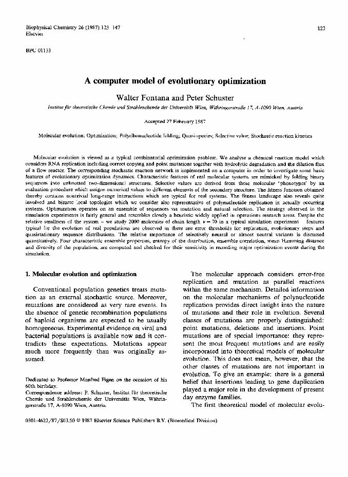
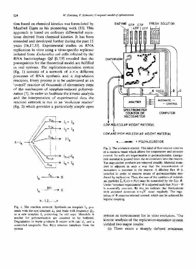
tion based on chemical kinetics was formulated by Manfred Eigen in his pioneering work [15]. This approach is based on ordinary differential equations derived from chemical kinetics. It has been extended and developed further during the past 15 years [16,17,35]. Experimental studies on RNA replication in vitro using a virus-specific replicase isolated from Escherichia co/i cells infected by the RNA bacteriophage Q/3 [6,7,9] revealed that the prerequisites for the theoretical model are fulfilled in real systems. The replication-mutation system (fig. 1) consists of a network of n x n different processes of RNA synthesis and n. degradation reactions. Every process is to be understood as an ‘overall’ reaction of thousands of elementary steps of the mechanism of template-induced polymerization [7]. In order to facilitate the kinetic analysis and the interpretation of experimental data the reaction network is run in an ‘evolution reactor’ (fig. 2) which provides a particularly simple open

A+Ik

‘Z+ lk

21k

ln-i+Ik

ln+ Ik

lk dk

ZB

*k OkI

.O

k= 1.2 ,....,.., n

Fig. 1. The reaction network. Synthesis on template I, proceeds with the rate constant uk and leads with frequency Q,k to a new template Ii preserving the old copy. Materials A needed for polymerization are assumed to be buffered. Degradation to waste products B occurs with rate d, and a controlled unspecific flux Q(z) removes templates from the system.

LO MbL ECULAR WEIGHT MATERIAL

1

ENZyME GTP CTP FRESH SOLUTION ,

--f AUTOMATIC - ANALYSER --f

- CONTROL

SPECTROMETER COUNTER OR

VISCOSIMETER COMPUTER

LOWAND HIGH MOLECULAR WEIGHT MATERIAL

l . . . . cma = POLYNUCLEOTIDE

Fig. 2. The evolution reactor. This kind of flow reactor consists of a reaction vessel which allows for temperature and pressure control. Its walls are impermeable to polynucleotides. Energy- rich material is poured from the environment into the reactor. The degradation products are removed steadily. Material trans- port is adjusted in such a way that the concentration of monomers is constant in the reactor. A dilution flux @ is installed in order to remove excess of polynucleotides produced by replication. Thus, the sum of the numbers of individual particles Z,X,(r) = N(t) may be controlled by the flux @. Under ‘constant organization’ 6 is adjusted such that N(I) = 0 is essentially constant. By this we indicate that fluctuations with standard deviation o =@ occur regularly. The regu- lation of 0 requires internal control, which can be achieved by logistic coupling.

system as environment for in vitro evolution. The kinetic analysis of the replication-mutation system yielded two major results:

(i) There exists a sharply defined minimum

W. Fontana, P. Schuster/Computer model of optimization 125

accuracy of replication below which sequences are dynamically unstable toward successive repli- cations. This instability implies that there is no long time correlation between sequences in the sense of heredity. Replication at low accuracy may be characterized, therefore, as ‘random replication’. We introduced the notion ‘error threshold’ for the transition from regular to random replication in order to indicate its sharpness in polymer sequences.

(2) Stationary states of a replication-mutation ensemble are characterized by distributions of sequences. These stationary distributions were called ‘quasispecies’ [17] in order to stress the analogy to the notion of species in biology. Quasispecies have precisely defined internal structures which are determined by the selective values of individual polynucleotide sequences and the mutation frequencies.

The conventional concept of natural selection has to be revised in the light of molecular biology. Not a single fittest type but an ensemble of sequences, the quasispecies, is selected. In this mod- ified form the selection concept prevails and evolution can be visualized as a succession of quasistationary states which are characterized as stationary solutions of the kinetic differential equations. Rare advantageous mutants eventually destabilize the quasistationary states. After a tran- sient phase the population reaches a new quasistationary sequence distribution. The evolutionary optimum is approached stepwise. We shall use the notion of ‘evolutionary steps’ for this phenome- non.

Some questions remain inevitably unanswered by the deterministic kinetic approach. Among them are those concerning the role of neutral mutations, the influence of population sizes on the selection process, and the factors which determine whether the evolutionary optimum is approached gradually or in steps. Still unsolved is the problem of how to predict whether or not a given replication-mutation system can approach the global optimum of the evolutionary process.

In order to be able to discuss some of the above-mentioned questions by means of a simple but as realistic as possible model system, we de- signed a computer simulation of optimization in

an ensemble of replicating RNA molecules. Although we intended to model the adaptive

behavior of a fairly simple and specific chemical reaction mechanism, it turned out that our model displays features which are very similar to those of a wide class of general optimization problems. Therefore, we make an attempt to formulate our optimization problem in general mathematical terms :

(1) We assume a (finite, nonempty) set E of K

different symbols, a, with i = I,. . ., K. In the case of polyribonucleotides we have K = 4 and a, E {G,A,C,U}; for binary sequences the specifica- tions are K = 2 and a, E (O,l}.

(2) The symbols are combined to strings of given length Y (Y t N). The set of all K” strings is denoted by

c’=c-c-c. . ..c. These strings represent the polynucleotide or binary sequences denoted by I, (k = 1, 2, . . . ,4’ or 2”, respectively). In the language of biology they represent the genotypes.

(3) Let u be a mapping that assigns a graph g, to every string I, = ajk)oJk) _. uJk) according to certain rules on the set of vertices { CJ,‘~‘; i = 1, 2,. . ., P}: g, = ~(1~). The graph g, is the phenotype corresponding to the genotype I,. In the case of polynucleotides or binary sequences I, is the primary sequence, i.e., the string of symbols a(“), and g, a secondary or tertiary structure formed according to the rules of base-pairing, in general some rules of symbol complementarity.

(4) Finally, we define a bounded function u( gk) which assigns a nonnegative value to every graph: wk = u(gk) = u(u{Ik}). In common biological terms, wk is the selective value or the fitness of the phenotype g,. The function u evaluates the phenotype g, which in turn is determined by the genotype I,.

The optimization problem can now be stated in the following form: find a string I, E E” such that the graph g, assigned to I, by u displays a maximum in u: w, = max(wk; k=l,...,~“}. In order to make the optimization problem numeri- cally tractable the computation of both functions u and IJ is assumed to be of polynomial time

126 W. Fontanu, P. Schwer/Computer model of oplimizacion

complexity in v which means that the number of individual computational steps is a polynomial in V.

The mapping u ( u { I}) is usually viewed as ‘cost’, ‘objective’ or potential function in the v-independent variables cri E E. In the relevant and interesting cases the cost function generates a quite com- plicated ‘landscape’ on the discrete polytope C which has been characterized as ‘sequence space’ [l&33]. In the case of binary sequences the sequence space is simply a hypercube of dimension v (fig. 3).

The cardinality of Y - this is the number of possible sequences, 4’ or 2’, respectively - for medium and large values of the chain length v (v > 200) exceeds by far the capacities of all re- sources, natural or artificial, be it a computer, a laboratory, a planet or even the physical universe. Thus, we are faced with a combinatorial optimization problem that reminds one of those belonging to the ‘nondeterministic polynomial time complete’ (NP-c) class. Any search has to aim at

‘good’, i.e., useful, solutions in acceptable amounts of space and time. A widely applied strategy in this context is ‘neighbourhood search’ or ‘best first and backtracking’ approach, in which the optimization proceeds via local improvements upon a restricted set of candidates until it gets stuck in a local or possibly global maximum.

Exactly the same problem arises when we trans- late the deterministic kinetic model of molecular evolution into a stochastic process on a finite population. An iterative heuristic in general optimization theory has a number of ‘knobs’, in our case rules which determine the rate constants, population size and replication accuracy, by which ‘fine tuning’ of the process can be achieved in order to obtain satisfactory performance. It is not surprising that the observed heuristic which operates in the evolution reactor is close to what might be characterized as ‘design by variation and natural selection’ (251. For example, this approach has been applied successfully to the travelling sales- man problem [26]. It also recalls ‘simulated-an-

v=s Fig. 3. The sequence space of binary sequences based on the two-letter alphabet (OJ). We present the case Y = 5. All pairs sequences, I, and IA with Hammin g distance d(i,k) =1 are connected by a straight line. The graph obtained is a hypercube dimension I = 5.

Of

of

W. Fontana, P. Schurter/Computer m&i of optzmizatton 127

nealing’ techniques as have been proposed by Kirkpatrick et al. [22]. The problem which we try to approach here has also much in common with Anderson’s [2] statistical analysis of spin glass Hamiltonians. He himself stressed this analogy in applications to polynucleotide replication and early evolution [3,32,37].

2. The computer model

2.1. The stochastic reaction network

The network of chemical reactions which we intend to simulate by stochastic events is shown in fig. 1. It describes reactions involving n polymers I, (k=l,..., n) and consists of n2 synthetic reaction channels (eq. l), n degradation channels (eq. 2) and n ‘improper’ reaction channels (eq. 3) representing an unspecific dilution flux Q(t):

Ak. Q,k I, - I, + I,

*cl) I, ----i 0. (3)

The numbers of polymer molecules are considered as stochastic variables X,Jr) which are in principle related to the conventional concentrations by averaging over many individual runs: [lk] = x,(r) = {X,(t)).

Pathway 1 is visualized properly as a succession of two different types of processes. The first step is the initialization of the polymerization process. We assume constant concentrations of all low molecular weight materials and we account for the stoichiometric kinetic contributions of these concentrations implicitly in the overall rate constants A, (k=l,..., a). After a sequence enters reaction channel 1 it completes the pathway by copying the template molecule. The template sequence I, = u1(k)@) ck) . . . a, thereby remains unchanged whereas the copy, in principle, may be any sequence I, (i = 1, 2,. . . , n). Here we shall follow a model which considers binary sequences of the same length Y (Ii E E”) [38]. Accordingly, only

point mutations are admitted. The copy is synthe- sized in many, precisely in V, reaction steps of the second type. These reaction steps describe the incorporation of individual digits into the growing copy chain. As polymerization proceeds along the sequence, the decision as to which digit is incorporated into the new strand has to be made at every position. Accuracy of replication is assumed to be uniform along the chain: the probability of mutation does not depend on the position in the sequence. In binary sequences the decision as to which digit is incorporated is restricted to two possibilities only. Incorporation of the correct digit, 0 + 0 or 1 + 1, occurs with probability 4. Then an error at a given position, that means incorporation of the complementary digit, 0 + 1 or 1 + 0, occurs with probability 1 -q_ The synthesis of a complete polymer is a series of simple Bernoulli trials which produces a mutant with m errors with a binomial probability density:

P,(v,q) = (;)@-“(I -q)“= (;jqv( 517

(4)

The individual mutation probabilities, which are the elements of the mutation matrix Q = { Qik}, can be written in the form

Qik = qy- W,W(l _ q)d(l*k), (5) where the Hamming distance of the two sequences Ii and I, is denoted by d(i,k). The mutation probabilities fulfil the conditions 0 2 Qj < 1 and I$Pki = IL-

Pathway 2 represents a specific intrinsic de- struction which corresponds to hydrolytic degradation. It occurs with a reaction probability Dk (k = 1, 2,. _.) n).

Pathway 3 models a self-controlled removal of sequences by an unspecific dilution flux such that the average total population number N(t) = xXk(t) approaches some fixed constant value

0 &d fluctuates around it. Then the unspecific flux is of the form

(6)

12x W. Fontma, P. Schuster/Computer model of optimization

A flow term as used in the deterministic equations,

k k

(6’)

is unstable in the stochastic treatment since it would lead to a divergent variance of the total population number N [21]. Every N(f) satisifies the constraint and hence the system is deprived of a regulating force which resets the original value of N after small fluctuations. The flow in eq. 6 instead introduces a self-regulating mechanism of the logistic type.

In essence, the stochastic simulation follows an algorithm proposed and applied to chemical reactions by Gillespie [19,20]. Let us now consider the stochastic events which lead to changes in the molecular content of the reactor. Each sequence I, (k = 1, 2,. _ , n) may enter one of the three reaction channels (a) with (Y E { 1,2,3}. The number of such events (for given k and a) in the time interval between t and t + At is counted by N,‘*‘(t, t + At). We then characterize all reaction channels by constants R, . (a) This means for example:

R(kl)= A,, RF)= D, and Ri3)= a(t).

Reaction probability densities P,$“)(t) are related to the ‘stochastic rate constants’ Rp’ such that the three relations

Prob{ Nia)(t,t + At) = 0) = 1 - R’,*‘.At + o(At)

(7)

Prob{ Nk(“)(t,t + At) = l} = R’,*)*At + o(At)

(8)

Prob{N,‘*)(t,t+At)>l} =o{At} (9)

hold for every reaction channel in the limit At --) 0. The stochastic series of events defined by eqs.

7-9 is a Poisson process and the probability density function is the exponential distribution with a reciprocal time constant Rp)

I$“‘( t) = R(kol) exp{ - Rp)t } (t > 0). (10)

Now we can easily implement the network of

events in the reactor. Since all choices of reaction pathways are independent Poisson processes, the whole network constitutes a compound Poisson process. By this we mean that the time t between two events of the combined process has a probability density

P(t)=R(t)exp{-R(t)t}, t>O

with

(11)

R(t) = c xRp)&(t) = k LY

(12)

Eqs. 11 and 12 define the internal clock of the reaction network. Intervals between successive events are independent, but obviously not identi- cally distributed because of the time dependence of the parameter R(t).

Given a time t = T at which an event occurs, which sequence (Ik) and which reaction channel ( CX) will be involved? Let Tk(=) be the time at which I, reacts according to (a) then we find by elementary probability arguments:

Prob{ 7”@ = t, Tts) >r(jzk, jkY)lT=t}

= Rj$/R( t). (13)

The implementation of the stochastic simulation on a computer is straightforward. It is described in detail in ref. 19.

2.2. The value function

The next problem is to define the rules according to which nontrivial sets of rate constants A, and D, (k = l,..., n) are generated from given sequence data. Thereby we intend to produce a value landscape which emulates some characteristic features of ‘real-life’ situations. According to what has been described before, this is done in two steps:

(1) The binary sequences I, are folded into secondary structures, which represent the ‘pheno-

W. Fontana, P. Schuwer/Compuier model of optimization 129

types’ gk in OUT model. The prediction of secondary structures of single-stranded nucleic acids has been the subject of numerous mathematical and algorithmic investigations since the problem was first approached in the early sixties [18]. Sys- tematic further studies led to the development of a number of elegant techniques which are based on dynamic programming [27,28,39-431 (for an ex- tensive list of references see ref. 42). The implementation used here follows the guidelines given in ref. 43. In order to make this contribution self-contained we describe the folding strategy in the appendix.

(2) The second step assigns rate constants Ak and Dk to the secondary structures, the phenotypes (gk) of the sequences I,. We chose two cases which differ with respect to sophistication of the value function.

(i) The simplest assignment would take directly the absolute value of the free energy of g, to be the replication rate constant, eventually after suitable scaling: A, = constant. 1 AG( gk) ( . Degrada- tion rates might be neglected: D, = 0. If a structure is unstable, AG(g,) > 0, then we set Aj = 0, the structure does not multiply and we are dealing with a ‘sterile’ variant. Since such a sequence would be diluted out of the reactor sooner or later, we may consider sterile variants also as ‘lethal within our model. The more stable a structure is in this simplest assignment, the higher is its selective value. The longer the stacking regions, the faster it will replicate. Clearly, this is biophysical nonsense since it contradicts experimental data on replication of single-stranded molecules. From the viewpoint of the mapping I, + g, -B (A,,D,), however, we are dealing with a problem of the same ‘universality class’ [3] as in the biophysically more appealing assignment discussed below. Moreover, we have the advantage of knowing a priori what the ‘fittest’ sequences look like: obviously they are the 32 palindromes with complete parallel stacks and variations only in the four digits of the hairpin turn (see the appendix). One series of computer experiments characterized as searches on the ‘thermodynamic value landscape’ was performed by assignments in this way.

(ii) The second assignment was chosen in order to meet better some biophysical constraints of

replication. Since up to now nobody knows how to calculate replication rate constants from secondary structures of single-stranded polynucleotides our model is only of heuristic value. It is based on the fact that replication operates on single strands [8] and that unzippering of helical regions is cooperative 1311. We assume that every stacking region slows down the overall replication process in an additive fashion and that the term each stack contributes is a sigmoidal function which is reminiscent of the Monod-Wyman- Changeux model:

Ak=tcR-tcl~ ny (1 + “jL))j

3 (l+ny))4+L (14)

The sum is to be taken over all stacking regions of the sequence Ik_ The njk) values refer to the lengths of the individual stacks: PZ~) denotes the number of base-pairs in the j-th stack of sequence I,. The parameter L is some large positive constant which determines the detailed shape of the sigmoidal curve. The parameters xR and ki represent rate constants: ICY is the replication rate constant of the linear unstacked chain whereas in - K1 corresponds to the limit of infinitely long stacks. Should a structure yield a negative rate constant A, < 0 then we declare the sequence as lethal and put A, = 0. The values of K~ and K, can be used, therefore, to control the fraction of lethal mutants.

The rate constants of the hydrolytic degradation, D,, are also made up of additive contributions from each unpaired region. Heavier penalties are assigned to free ends and joins than to loops. There is no cooperativity.

s(k)

+‘Cy. 1

The first sum herein is taken over all loops, the second over all external elements as there are joins and tails. Three rate constants, K~, K~ and K~, are introduced to determine stability against hydrolysis. The number of unpaired digits in the j-th loop

130 W. Fontam, P. Schuster/Compuier model of optimrantron

of sequence Ik is denoted by uj”), the length of the I-th unpaired element in the same sequence by VI (k); U m is a weighting factor and v the length of the sequence.

All we have to do now is to ‘parse’ the folded secondary structure g, of the sequence I, into its elements in order to obtain the information needed in the computation of Ak(gk) and Dk(gk). The selective value or fitness factor of the sequence I, is then computed from W,, = A,. q” - D,.

We characterize this second assignment of fitness factors to the secondary structures gk as ‘ kinetic value landscape’. Certainly, our evaluation of rate constants from structural elements is naive in the light of modern biophysics but we do not aim at a quantitative determination here. In- stead, we present an example of an assignment in which high fitness is based on a compromise between two contradictory trends: long double-helical regions stabilize against hydrolysis, but they also reduce the rate of replication and vice versa. Some details of the value landscapes in the thermodynamic and kinetic case are discussed in section 3.

2.3. The data structure

The last question we have to address here is that of suitable data structures in order to keep track of the current sequence distribution in an evolving population. Repeatedly we search the population for the appearance of mutants and adjust their counters or in the case of new sequences we start the folding procedure. Folding has to be kept to a minimum since it represents the most time-consuming step of the whole simulation. Therefore, we need a data structure which supports efficient searching and allows one to insert and delete specified items. The nature of the process suggests, moreover, that insertions of new sequences and deletions of obsolete ones occur far from random. We have to avoid structures in which those operations interfere strongly with their search properties.

An elegant data structure that performs all operations required on N items in guaranteed O(logN) time complexity was devised in the early sixties [l]. It is known as the celebrated balanced

binary tree method [23]. The search tree is balanced by a set of rotation operations whenever the height differences between right and left subtrees exceed some critical value upon insertion or dele- tion. We chose the balanced tree especially with regard to future experiments with variable chain lengths, since many independently growing and shrinking trees can easily coexist in one large internal storage pool.

3. Value landscapes

Before we discuss the results of computer simulations we present some data on general structures of the two types of value landscapes. First, we consider the distribution of selective values and explore the value landscape by a Monte Carlo search. We begin from the ‘all-zero’ sequence I, of chain length v = 70, the sequence which consists of seventy digits 0 exclusively, and replace the digits 0 by digits 1 at every position with a given constant probability 4. Thereby we obtain a random distribution of sequences of almost Gaussian shape which is centered around the (70 X q)-error mutants of the reference sequence I,. Apart from some minor details a random sample of 38000 different sequences was sufficient to reflect the general features of the fitness landscape. Repeats with 76000 trials showed almost no detectable differences.

The distributions of selective values were calculated for three different q values, ql = 0.2857, q2 = 0.5 and q3 = 0.7143, which led to mutant distributions centered around the 20-, 35- and 50-error mutants of the all-zero sequence I,,. Three different parts of the sequence space were ex- plored in such a way. The value landscape for the thermodynamic assignment differs significantly from that of the kinetic model (fig. 4).

The selective values in the thermodynamic assignment show roughly a ‘noisy’ Gaussian distribution. The mean selective values for q1 and q3 me about the same: p= 500 (t-i) (Selective values are rate constants by definition [16,17] and therefore are given in reciprocal arbitrary time units here). The distribution around the 35-error mutants is significantly superior: W= 750 (tt’).

W. Fontma, P. Schuster/Computer model of optimization 131

> t- m

6 P

012

010

008

006

004

002

0.

0 1000 2000 3000

FREE ENERGY

0 1000 2000 3000 -1000 D 1000

FREE ENERGY EXCESS FRODUCTION

-1DOO 0 1000

EXCESS PRODUCT1 ON

*.0015 t-

2 ;.0010

.ooos

0.

Fig. 4. Distribution of selective values in sequence space. 38ooO different sequences of length Y = 70 were generated by introducing digits 1 at random with probability q1 = 0.2857, qz = 0.5 and q3 = 0.7143. This produces samples of Gaussian shape centered around the 20., 35- and SO-error mutants of the ah-zero reference sequence. The distributions of the free energy AGk and the excess production A, - D, are shown for the regions located at mean Hamming distances 35 (upper plots) and 20 (lower plots) from the all-zero vertex of the hypercube. Apart from a scaling factor the free energy distribution constitutes the thermodynamic fitness landscape. For high-accuracy replication (e.g., for all runs reported in the text) the kinetic fitness landscape retains the same shape as the (Ak - 4) distribution. The densities in the surroundings at distance 50 (not shown) are essentially the same as those at distance 20. They contain the direct (i.e., unchanged polarity or folding direction; the common plus-minus complementarity is inverse complementarity, since the polarity of the minus strand is opposite to that of the aligned plus strand) complementary sequences. Although the secondary structures of sequences directly complementary to each other differ in general, the pools of configurations derived from them behave in the same way with respect to evaluation.

lnterpretation of this observation is straightforward. The 35-error mutants have as many digits 0 as digits 1 and, provided the primary sequence admits it, they form more base-pairs than the 20- or SO-error mutants do. In essence, therrnody- namic stability counts the number of base-pairs and hence, the 35-error mutants of the all-zero

sequence I, are the most stable on average. A plot of the distributions on the kinetic landscape is shown for the case 4 = 1 where the selective value becomes identical to the excess production E, = A, - D,. In the case of the distributions around 20- and 50-error mutants we observe an interesting bimodal shape. Bimodality is here a result of

132 W. Fonram. P. Schuster/Computer model of optimization

the relation between A, and D, values as regu- lated by eqs. 14 and 15 and will be discussed in detail in a forthcoming paper.

It is useful to split the kinetic landscape into the different contributions resulting from replication and degradation rate constants (fig. 5). The distribution of the degradation rate constants and the thermodynamic value assignment have much in common. Degradation rate constants also re- semble noisy Gaussian distributions. This is no surprise since both functions roughly count the numbers of base-pairs, eventually with slightly different weightings. Obviously the dependence on

.DlZ

.I310

008

c z 006

41 ,004

.ooz

0.

.u12

,010

.008

c VI .006

! ,004

.002

0

1000 2000 3000

REPLICATION CONSTANT

0 1000 2000 3000 0 1000 2000 3000

DEGRADATION CONSTANT DEGRADATION CONSTANT

A B

the number of base-pairs formed is opposite: many base-pairs imply high thermodynamic stability but low rate of degradation. By the same token the 35error mutants hydrolyse less readily than the 20- or 50-error mutants do.

The distribution of replication rate constants, shown in fig. 5, differs rather drastically from the other two. It looks bizarre and determines the overall shape of the total kinetic value landscape. Due to the sigmoidal contribution of the lengths of double-helical regions replication rates are extremely sensitive to minor details of the structure and this leads to an enormous scatter in the distri-

c Lo ,006

6 0

004

,002

0

0 1000 2000 3000

REPLICATION CONSTANT

Fig. 5. Splitting of selective values on the kinetic surface into replication rates A, (upper plots) and degradation rates Dk (lower plots). Parts A and B show the distributions sampled from the 35- and 20-error environments, respectively, as explained in the caption to fig. 4. Note that in the upper plot of (A) the high density (0.18) at A, = 0 has been cut off to show the details of the surface at positive rates.


bution. Long base-paired regions are a disad- vantage for replication and therefore, 20- or 50-error mutants of the all-zero sequence I,, replicate faster on average than the 35error mutants do. The latter region of the sequence space bears many structures with some stacks above the critical length of four to five base-pairs. Due to our particular choice of the constants K~ and K~ in eq. 14 the contributions of these stacks cumulate to a negative replication rate constant which is set at zero, thus establishing a nonviable mutant. The fraction of nonviable sequences in the sample centered around Hamming distance 35 is therefore

620

600

580 560

Y ;: 540

id 520

I 500

0 10 20 30 40 50 60 70

MUTATED POSITION

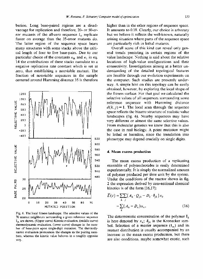
Fig. 6. The local fitness landscape. The selective values of the 70 nearest neighbours surrounding a given reference sequence I, are shown. (Upper curve) Kinetic evaluation, (middle curve) thermodynamic evaluation, (lower curve) changes in the number of base-pairs upon single-digit mutation. The thermodynamic evaluation pronounces the changes in the pairing numbers, whereas the kinetic value behaves in a roughly opposite way.

higher than in the other regions of sequence space. It amounts to 0.18. Clearly, our choice is arbitrary but we believe it reflects the well-known, naturally arising situation where parts of the sequence space are particularly rich in lethal mutants.

Overall scans of this kind can reveal only general trends persisting in certain regions of the value landscape. Nothing is said about the relative locations of high-value configurations and their connectivity. Investigations aiming at a better understanding of the detailed topological features are feasible through our evolution experiments on the computer. Such studies are presently under- way. A simple hint on this topology can be easily obtained, however, by exploring the local shape of the fitness surface. For that goal we calculated the selective values of all sequences surrounding some reference sequence with Hamming distance d( k, j) = 1. The local scan through the sequence space reflects the bizarre structure of realistic value landscapes (fig. 6). Nearby sequences may have very different or almost the same selective values. From molecular genetics we know that this is also the case in real biology. A point mutation might be lethal or harmless, since the translation into phenotype may depend crucially on single digits.

4. Mean excess production

The mean excess production of a replicating ensemble of polynucleotides is easily determined experimentally. It is simply the normalized amount of polymer produced per time unit by the system. Under the conditions of the reactor shown in fig. 2 the expression derived by conventional chemical kinetics is of the form [16,17]:

kj

k

The deterministic concentration of the polymer I, is here denoted by x,; 6;k is the Kronecker symbol. Selection of a master sequence (I,) and its mutant distribution is usually accompanied by an increase in the mean excess production, but there are also conditions, maybe somewhat exotic, such

134 W. Fontam, P. Schuster/Computer model ~Juptimizntion

as commencing with the pure master sequence I,,,, for which E(t) decreases or does not even behave monotonically [34]. In any case it approaches a well-defined asymptotic value which is determined by the inequality

A,-D,,,> lim~(t)=E,z-A;Q,,-D,,,. I-+W

(17)

The difference between the selective value of the master sequence and the asymptotic mean excess production is a measure of the total fraction of revertants; these are mutations leading from mutants back to the master:

08)

The master sequence is well defined in a stationary mutant distribution as the most frequent sequence which is commonly characterized by the largest selective value. In the stochastic computer simulations we are not dealing with stationary populations and therefore we have to generalize the concept. The notion master sequence is re- tained for the most frequent type irrespective of

selective value.

The results of seven typical selected runs are shown in figs. 7-9 and 11. In order to facilitate reading the individual runs are denoted con- sistently by letters: A-G. Ail computer experiments reported here use a chain length of v = 70, an average population size of F= 2000 and start from a homogeneous population. There is a rather fast initial period during which a first mutant distribution is formed. Then optimization starts. When a simulation starts from a very inefficient initial sequence it turns out to be necessary to evaluate selective values in the first phase differ- ently from the genuine simulation experiment in order to avoid negative mean excess production. This has been done by generally slowing down degradation without altering the shape of the fitness surface.

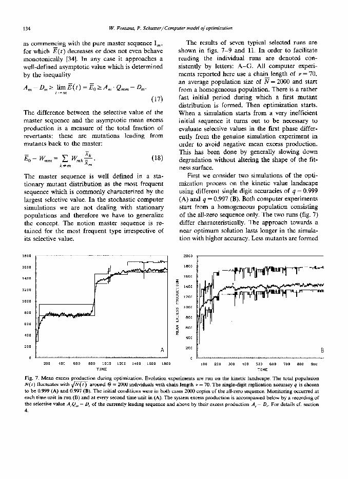
First we consider two simulations of the optimization process on the kinetic value landscape using different single digit accuracies of q = 0.999 (A) and 4 = 0.997 (B). Both computer experiments start from a homogeneous population consisting of the all-zero sequence only. The two runs (fig. 7) differ characteristically. The approach towards a near optimum solution lasts longer in the simulation with higher accuracy. Less mutants are formed

Fig. 7. Mean excess production during optimization. Evolution experiments are run on the kinetic landscape. The total population N(I) fluctuates with $qq around 8 = 2000 individuals with chain length P = 70. The single-digit replication accuracy q is chosen to be 0.999 (A) and 0.997 (B). The initial conditions were in both cases 2000 copies of the all-zero sequence. Monitoring occurred at each time unit in run (B) and at every second time unit in (A). The system excess production is accompanied below by a recording of the selective value A,Q,, - 0, of the currently leading sequence and above by their excess production A, - D,. For details cf. section 4.

W. Foniana, P. Schuster/Computer model of optimmztron 135

and optimization is less efficient. In the high-accuracy case we also observe quasistationary state which lasts roughly from f = 200 to r = 800. Sub- sequently, the mean excess production increases instantaneously. We observe an evolutionary step. In the low-accuracy simulation such a step is vaguely indicated only between t = 100 and t = 200. Another obvious consequence of the mutation rates concerns the difference E- W,, in the stationary state which is a measure of the relative importance of revertants. This difference is sub- stantially larger in the run at lower accuracy where the frequency of mutation is higher.

Next we consider two computer experiments on the kinetic value landscape, C and D, starting from a sequence (fig. 10) which is less far away from a ‘near-optimum’ solution than the all-zero sequence. The results are shown in fig. 8. Clearly, a nearly optimal sequence is approached faster than in the two previous runs. Again, the simulation with higher replication accuracy (C: 9 = 0.999) shows a detectable evolutionary step in the optimization process, whereas the other run (D: 4 = 0.997) approaches the optimum gradually. The asymptotic value of the difference E- W,, behaves as expected: it is larger for D (4 = 0.997) than it is for C (4 = 0.999).

Two other simulation experiments (E and F) .

were carried out on the thermodynamic landscape (fig. 9). Both commence from the same sequence (fig. 10) and use the same q values as the previous sets of experiments. On the whole optimization is somewhat faster on the thermodynamic landscape than it is on the kinetic one. It is also ‘smoother’ in the sense that practically no evolutionary steps can be detected. The less accurate simulation reaches a near-optimum sequence faster than the more accurate computer experiment does. In this particular example we are in the position to predict the sequence with maximum selective value (fig. 10). It is a perfect hairpin, a hairpin with the maximum number of base-pairs, here 33, with ‘0 digits on one side and ‘1’ digits on the opposite side. Changes within the four digits of the loop give rise to a family of selectively neutral variants. The simulation at lower accuracy (4 = 0.997) reaches a perfect hairpin within the time spent in the run. It is not yet the global optimum but it contains the maximum number of base-pairs. The high-accuracy run (q = 0.999), however, becomes stuck in a nonoptimal hairpin with one base-pair less.

Let us now consider a ‘downhill’ computer experiment on the thermodynamic landscape (G) where we start from the optimum sequence and follow the decay of the population due to mu-

Fig. 8. Mean excess production during optimization. The recordings of runs with q = 0.999 (C) and q = 0.997 (D) under reactor conditions as described in fig. 7 are shown together with the selective values of the leading sequences. We started from a homogeneous population of the sequence shown in fig. 1OA.

136

,200

,100

1000

5 i: 300 3 2 600

% z 700

z 600

H 500

400

300

200

W. Fontana, P. Schuster/Computer mode/ of optrmrzalion

E

1300

1200

1100

1000

900

BOO

700

600

500

400

300

200 F

0 50 100 150 200 250 300 350 400 450 0 50 LOO 150 200 250 300 350 400 450 TIME TIUE

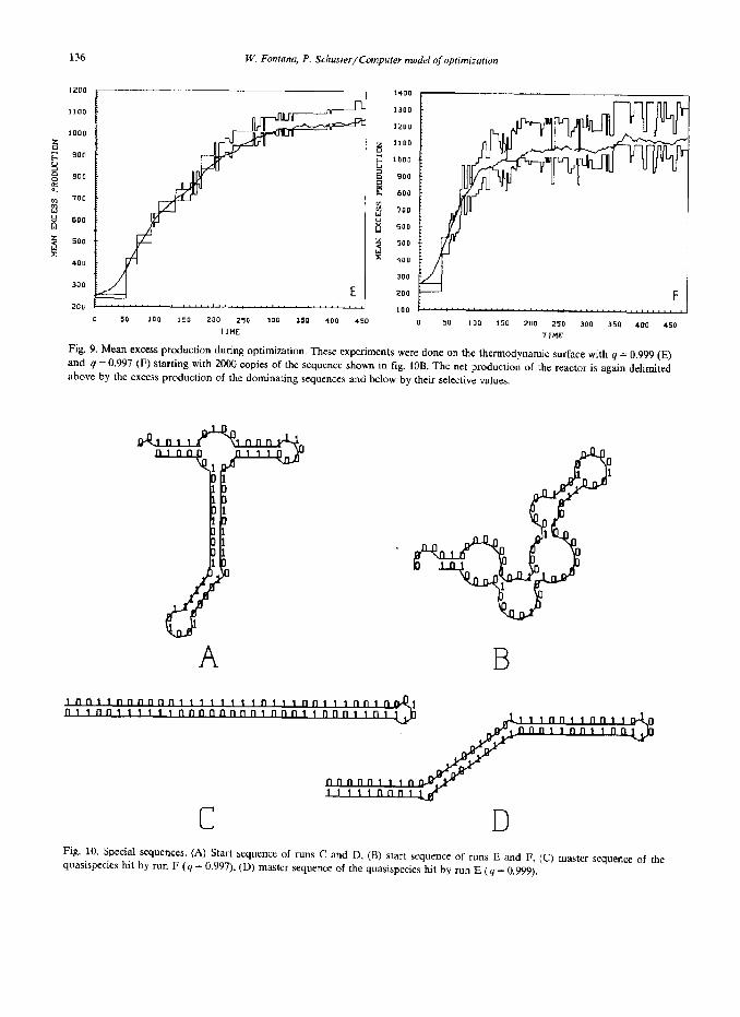
Fig. 9. Mean excess production during optimization. These experiments were done on the thermodynamic surface with 4 = 0.999 (E) and 4 = 0.997 (F) starting with 2000 copies of the sequence shown in fig. IOB. The net production of the reactor is again delimited above by the excess production of the dominating sequences and below by their selective valuea.

Fig. 10. Special sequences. (A) Start sequence of runs C and D, (R) start sequence of runs E and F, (C) mater sequence of the quasispecies hit by run F (4 = 0.997), (D) master sequence of the quasispecies hit by run E (4 = 0.999).

W. Fontana, P. Schuster/Computer model aj optimization 137

G I

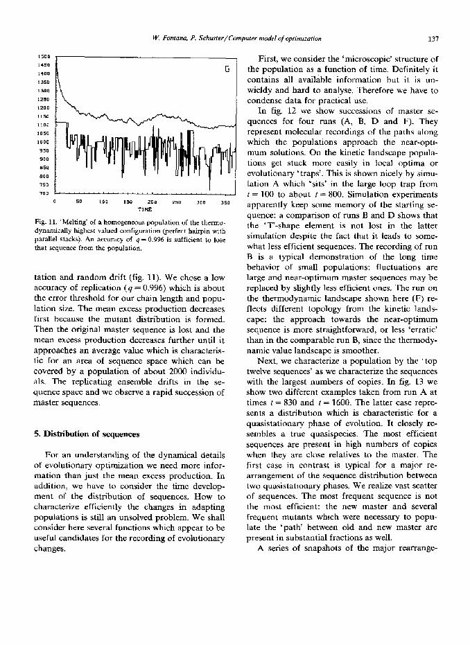
Fig. 11. ‘Melting’ of a homogeneous population of the themo- dynamically hxghest valued configuration (perfect hairpin with parallel stacks). An accuracy of 4 - 0.996 is sufficient to lose that sequence from the population.

tation and random drift (fig. 11). We chose a low accuracy of replication (4 = 0.996) which is about the error threshold for our chain length and population size. The mean excess production decreases first because the mutant distribution is formed. Then the original master sequence is lost and the mean excess production decreases further until it approaches an average value which is characteristic for an area of sequence space which can be covered by a population of about 2000 individuals. The replicating ensemble drifts in the sequence space and we observe a rapid succession of master sequences.

5. Distribution of sequences

For an understanding of the dynamical details of evolutionary optimization we need more information than just the mean excess production. In addition, we have to consider the time development of the distribution of sequences. How to characterize efficiently the changes in adapting populations is still an unsolved problem. We shall consider here several functions which appear to be useful candidates for the recording of evolutionary changes.

First, we consider the ‘microscopic’ structure of the population as a function of time. Definitely it contains all available information but it is un- wieldy and hard to analyse. Therefore we have to condense data for practical use.

In fig. 12 we show successions of master sequences for four runs (A, B, D and F). They represent molecular recordings of the paths along which the populations approach the near-optimum solutions. On the kinetic landscape populations get stuck more easily in local optima or evolutionary ‘traps’. This is shown nicely by simulation A which ‘sits’ in the large loop trap from t = 100 to about t = 800. Simulation experiments apparently keep some memory of the starting sequence: a comparison of runs B and D shows that the ‘T’-shape element is not lost in the latter simulation despite the fact that it leads to somewhat less efficient sequences. The recording of run B is a typical demonstration of the long time behavior of small populations: fluctuations are large and near-optimum master sequences may be replaced by slightly less efficient ones. The run on the thermodynamic landscape shown here (F) reflects different topology from the kinetic landscape: the approach towards the near-optimum sequence is more straightforward, or less ‘erratic’ than in the comparable run B, since the thermodynamic value landscape is smoother.

Next, we characterize a population by the ‘ top twelve sequences’ as we characterize the sequences with the largest numbers of copies. In fig. 13 we show two different examples taken from run A at times t = 830 and t = 1600. The latter case represents a distribution which is characteristic for a quasistationary phase of evolution. It closely resembles a true quasispecies. The most efficient sequences are present in high numbers of copies when they are close relatives to the master. The first case in contrast is typical for a major rearrangement of the sequence distribution between two quasistationary phases. We realize vast scatter of sequences. The most frequent sequence is not the most efficient: the new master and several frequent mutants which were necessary to popu- late the ‘path’ between old and new master are present in substantial fractions as well.

A series of snapshots of the major rearrange-

138 W. Fontann, P. Schurter/Computer model of optimizntron

ment of the sequence distribution at the evolutionary step in run A is shown in fig. 14. The sequence distribution centered around the new master builds up as the old quasispecies-like distribution decays.

A

T-O Q T_4aQ

T-34 E-486

T-1 024 T-1052 E-l 578 h-1628

B

T-O T-32

T-137 E-1460

T-232 T-325 0 E-1719 E-1769

T- 1284 E-l 692

T-69 E-1179

n

J T-142 E-1437

1 T-363 E-1722

T-6?+j ..6?$ T-9h E-1766 E-1759 E-1798

Moreover, we realize intermediate sequences posi- tioned on an ‘island’ in sequence space which has to be populated before the evolutionary jump of the ensemble becomes possible.

D T-90 T-04 E-71 5 E-943

\ T-840 E-1480

T-70 E-1455

\ T-160 E-1616

T-103 E-l 355

T-170 E- 1677

r T-200 E-171 1

T-367 T-417 \ T-456 E- 1762 E- 1674 E-1740

T-91 1 v T-913 b T-951 D E-1750 E-1798 E-1777

Fig. 12. Selected recordings of the successions of master sequences along the path to the final distribution. A, B, D and F denote the corresponding runs reported in the text (T = time, E = A - D = net production).

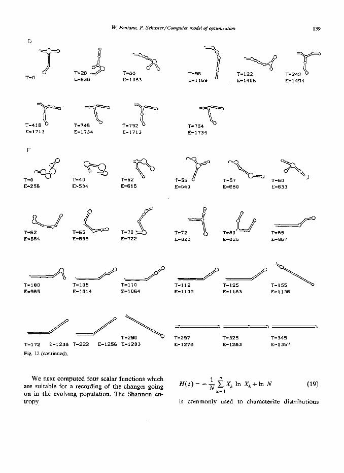
W. Fontma, P. Schuster/Computer model of optimization 139

T-O E-830 E-1083 T-96 7 E-l 169 E-1406 E-1494

T-4lr T-74T T 75r _ E-171 3 E-1734 E-1713

T-O ” T-40 T-52 ” E-256 E-534 E-616

E-664 E-696 E-722

E-640 T-57 E-680

E-826

T-100 E-gas

T-105 T-110 T-112 T-125 E-1014 E-1064 E-1109 E-l 183

T-60 J

E-633

T-85 E-967

\ T-155 E-1136

J /T-l T:T:T: T-172 E-1238 T-222 E-1256 E-1203 E- 1278 E-1283 E-1357

Fig. 12 (continued).

We next computed four scalar functions which are suitable for a recording of the changes going H(t) = +XkInXk+lniV (1% on in the evolving population. The Shannon en- k-l

tropy is commonly used to characterize distributions

140 W. Fontana, P. Schuster/Computer model of optimizotinn

“_743cJlo4?+QLlo73~ c-199 c-35 c-62 d-0 d-16 d-17

il -4 v-1307 v-705 v-l 062 c-59 c-52 c-43 d-21

v-916 c-37 d-16

d-16 d-17

d-l d-20

v-734 2 _g63~“-g53 4 c-25 d-17

c-25 c-23 i-J d-19 d-18

T= 830

V v-l 516 c-166 d-0

c-112 d-6

c-65 d-2 Yl

v-l 504 c-61 d-4

v-1443 c-41 d-5

;I

v-l 504 c-40 d-l

v-l 504 c-57

d-3 c

v-1516 c-45 d-l

Q

v-1501 c-41 d-8

\ v-1480 c-40 d-2

v-l 504 c-36 d-3

T=1600

Fig. 13. The twelve most frequent types (‘top twelve’) at times T = 830 and T = 1600 of run A. At T = 830 the ensemble is rearranging internally for the jump shown in fig. 7 (A); at T = 1600 a typical quasistationary state is achieved. U, Selective value; c, number of copies; d, Hamming distance from the most frequent type.

and has also been applied to molecular populations [lO,ll]. Characteristic examples are shown in fig. 15. As expected the entropy is larger if replication is less accurate. The perfect evolutionary step of the high-accuracy run (A) shown in fig. 7, however, is not well documented by the entropy function. We realize the spontaneous increase after

t = 800 but then the function settles at a value which is almost as large as that during the major rearrangement.

The second function to be considered here is a kind of autocorrelation function of the (nonsta- tionary) sequence distribution. We call it ‘ensemble correlation’ since it represents a measure for

~- _.-~~- Fig. 14. Rstabilization of a quasispecies and building up of a new quasistationary state. The optinwation jump in run A is resolved into frequencies of selective values at different Hamming distances computed from the new outgrowing master sequence. At time T = 700 the ‘newcomer’ has not yet appeared in the system, but 120 time units later a path to it has been established. The resolution along the value axis is of 10 units, i.e., the frequencies of types with values u E (u k ~ 5, ok + 5), for some IJ~, are cumulated. Clearly, care has to be taken in inferring the relative distances in the Hamming metric between peaks not involving the new master at d = 0. The btghest peak at time T = 700 amounts to 0.29. It was cut off at 0.2 in order to make the smaller peaks better visible

W. Fonrana, P. Schurter/Computer model oj optimizolion

T= 840

141

.20

T- 820 T= 850

.05

0. 0. DO

0

.05

0. 00 00

0

W. Fontma, P. Schuster/Computer model of optimization

c?(t, At) = {J?(r + At) *z(t))

= + &t+At).x,(lj. (20) k L

in contrast to an ordinary autocorrelation function, we consider a fixed time increment (At) and analyse the ensemble correlation as a function of t. We calculated C(t,At) for several choices of At but it turned out that the correlation function is not at all sensitive to this choice. Clearly, the ensemble correlation is unity in a stationary (deterministic) population. Any real population, however, is always ‘quasistationary’. By this we mean that only the master sequence and the most frequent mutants are present in constant fractions of the total population. There will be rearrangements at the periphery of the quasispecies-like distribution. Therefore, c( t, A t) will be less than unity. The quantity 1 - c( t, At) is a direct measure of the importance of fluctuations at the periphery. In fig. 16 we show two characteristic examples of ensemble correlation functions. They turn out to be a useful diagnostics for major rearrangements of sequence distributions occurring at evolutionary steps: C(t,At) drops before the midpoint of the rearrangement. The two correlation functions

0 200 400 600 a00 1000 1200 1400 ,600 ,800

TIHE

15. The Shannon entropy (eq. 19) of runs A and B. The recording for run A shares some vague shape features with the mean Hamming distance of fig. 17 (A), whereas the upper curve for the less accurate run B lacks the ability to monitor the adaptive behavior of the system.

rearrangements of the distribution within a given time interval At. We describe the seauence distribution by a vector T(t) = (X,(t), X2(t), . . . , X, (t >}. Then, the ensemble correlation is defined as

1.00

.99

-96

.97

-96

.95

.%

-93

.92

-91

.a0

1.00

0 zoo 400 600 600 1000 ,200 1400 1600 l800 0 200 400 600 BD(I I

TIHE TlHE

Fig. 16. The ensemble correlation (eq. 20). The series of projections between states At = 2 time units apart from each other is shown for run A (left) and for run B (right). For details cf. section 5.


for runs A and B with different accuracy differ characteristically. There is almost no change in the population during the early period (200 -C t -C 800) of the high-accuracy simulation. Then we observe three noisy drops corresponding to evolutionary steps before the population settles around a mean value of c(t, At = 2) = 0.97. The run at lower replication accuracy shows only one drop before it settles at a mean value of C(t,At = 2) = 0.89 re- flecting higher mutational activity.

A

0 200 400 600 800 LOO0 1200 ,400 1600 ,800 TIME

El

0 200 400 500 800 1000

TINE

Fig. 17. The mean Hamming distance (eq. 21). This measures sensitively the width of the current state in the appropriate metric of the hypercube. The upper part has been traced during run A, the lower one during run B. For details cf. section 5.

Another global function of sequence distributions which turned out to be useful here is the mean Hamming distance defined by

so

45

.40

.35

i .30

8 .25

2 q .20

.I5

.I0

.05

0.

0 200 *00 600 800 1000 1200 1400 1600 181

TIHL

Fig. 18. The diversity {eq. 22). This measures the support on which a sequence distribution is built. Inheritance keeps a kernel of the sequence distribution away from dropping below the threshold of stochastic noise. This implies a restriction upon the band width of the variability that can be sustained in a given evolutionary system under defined conditions. The diversity obviously depends upon the replication accuracy 4, but it also depends on the topology of the fraction of the fitness surface that is occupied instantaneously by the ensemble. We observe a characteristic grouping of the diversities according to the chosen simulation conditions. High-accuracy runs (A, C, E) show a lower diversity than the low-accuracy experiments (B, D, F, G). Simulation G is just below the error threshold, which is reflected by a fraction of sequences differ- ing from each other as high as 0.44 on average. Runs C and D start from a different region in sequence space than A and B and settle on a different diversity. The same holds for a comparison between the runs on the kinetic surface (A, B, C, D) and the experiments with the thermodynamic evaluation (E, F). The latter landscape seems to produce more variability under comparable conditions. This may be due to a higher density of neutral mutants resulting from the smoother surface. This is viewed as a hint that the error threshold depends in fact on the actual value landscape. The pronounced evolutionary step in run A swaps the ensemble from a location near the all-zero vertex of the hypercube to another far away from the starting point. The corresponding change in the otherwise constant diversity hints at a different topology of the value surface in that region. In addition, the diversity also depends on population size.

144 W. Foniana, P. Schuster/Computer model of optimization

Two typical examples of mean Hamming distances in simulations with different accuracies are shown in fig. 17. The mean H amming distance increases sharply at evolutionary steps. In quasistationary populations it fluctuates around mean values which are measures of the widths of mutant distributions. In our particular examples we found 3 = 7 in the more accurately replicating population with q = 0.999 and B = 11 in the population with q = 0.997. The last of the four global quanti- ties of sequence distributions which we discuss here is the diversity V(f). It is a measure of the width of distributions and simply counts the number of mutants present:

V( t ) = $ . (number of mutants present at time t ) .

(22)

Accordingly, the diversity is unity in a population in which all sequences are different. It is l/N in a uniform distribution. As seen from the examples shown in fig. 18, the diversity is an appropriate measure for the characterization of quasistationary populations. High diversity implies high capacity for evolutionary adaptation provided the system is still above error threshold. Below error threshold the diversity is large and may approach unity.

6. Conclusions

Populations of a few thousand molecules, which are about the size we can handle with our computational facilities, are minute compared to population sizes commonly used in microbiology or in test-tube evolution experiments. When we de- signed our simulation studies it was not at all clear, therefore, whether we would be able or not to observe typical evolutionary phenomena as there are error thresholds, quasistationary mutant distributions or evolutionary steps. Fluctuations might cover the interesting features. The computer experiments have shown that this is not the case. Error thresholds, originally derived for infinite populations, do exist in small populations as well, The influence of population size on error thresholds is unclear. Intuitively, one would expect that

higher accuracy is needed in smaller populations to sustain stable ensembles of replicating sequences since fluctuations are more likely to wipe out individual types there. The structure of the value landscape, of course, also has an influence on the error threshold. As the simulations have shown, the error threshold for a population of 2000 individuals of chain length v = 70 on the thermodynamic landscape lies somewhere in the range 0.996 i q_ < 0.997. A ‘conservative’ esti- mate of the deterministic error threshold on this energy surface yields q_ = 0.990 for v = 70.

Depending on chain length, population size and structure of the value landscape, an efficient approach towards a target sequence of optimum or near-optimum selective value requires an optimum replication accuracy. Too high an error rate, as shown by the downhill experiment in fig. 11, leads to continuous loss of the most efficient sequences. The population is unable to adapt and scans the sequence space in the manner of a random walk. The mean excess production therefore reaches only an average value of the area populated in sequence space. Clearly, too low a replication accuracy is prohibitive for evolutionary optimization because there is no long time correlation between sequences in the sense of inheritance.

Too high an accuracy of replication, on the other hand, slows down the optimization process. The ensemble eventually becomes stuck in a local optimum of the fitness landscape. Before we reach a situation in which the system is locally bound for long times we encounter quasistationary states and evolutionary steps. The replicating ensemble resides temporarily at a local trap on the value landscape. An example of this kind is shown in fig. 7. It is possible to interpret the occurrence of the step on the molecular level. The quasistationary distribution before the step consists mainly of sequences with one large loop (fig. 12). No much more efficient sequences lie in the direct surrounding of the large-loop-structures, since at least one stem has to be formed within an all-zero region and this requires several point mutations at a time. If the error rate is low, formation of a many-error mutant is an unlikely event.

The best-documented experimental record of an evolutionary step has been reported for the Q/3

W. Fontann, P. Schwrer/Computer model of optimization 145

system [24,36]. The environmental conditions for replication of the MDV-1 variant of Q/3 RNA, a small polyribonucleotide with Y = 218, deterio- rated on addition of ethidium bromide to the stock solution. The mean excess production drops immediately and stays for about six serial trans- fers at the low value before it increases in a stepwise manner. This can be easily interpreted by means of the results shown in fig. 7: the replication accuracy of Qp replicase (q = 0.9997) is extremely high for the chain length of the RNA molecule (v = 218) and hence only few mutants are present at the quasistationary state. The population proceeds through a succession of transients dominated first by a one- and then by a two-error mutant until it reaches a new quasistationary state in which the most efficient variant is a three-error mutant of the original master sequence. All four sequences were isolated and identified by sequence analysis.

Sequence data are now readily obtained for viruses and bacteria. The new techniques allow detection of sequence heterogeneities in natural populations [13,14,29] and determination of mutation rates [5,12,30]. How to collect data efficiently and how to derive the desired information on the evolutionary optimization process are still not known. We made an attempt to evaluate several functions which might serve as a diagnostics for the microscopic state of the system. The mean Hamming distance was found to be the best indicator of major rearrangements of sequence distributions. Information on the status of quasistationary sequence distributions is obtained much more easily. All four functions provide a direct measure of the spreading of the population in sequence space.

Finally, we return to the optimization problem and the structure of the value landscape. Two different types of phenotype evaluation were applied in the computer simulations reported here. Although the kinetic and thermodynamic landscapes differ in significant details, they have common properties which are of major importance for optimization. The local structures are bizarre. The selective values at nearby points in sequence space may be very different. There is plenty of room for selectively neutral or slightly deleterious mutants

which are responsible for the spreading of distributions. The efficiency of optimization is determined by the accuracy of replication. An optimum strategy with constant accuracy of replication is to operate as closely as possible to the error threshold in order to allow fast adaptation and to reduce the danger to be caught in a local fitness trap. It is also straightforward to conjecture a near-optimal strategy with adjustable mutation rates:

(1) Operate close to threshold during the major phases of optimization.

(2) In order to avoid local fitness traps, reduce the accuracy below threshold whenever the system stays for longer time in a quasistationary state. Then, after the trap has been passed return to the slightly above threshold strategy and stick to it as long as sufficient progress is made in optimization.

This strategy is the basis of a research program developed by Manfred Eigen and co-workers [l&16] which aims at optimization of biopolymers. It is also a straight analogy to the well-known simulated annealing technique [22].

Appendix: The strategy of folding

The secondary structure of a sequence I can be defined in the following formal way [401: Given a sequence I = ~~(7~. . . CT, the secondary structure is a graph g on the set of the IJ labelled points 1% cZ,, . . , a,} such that the adjacency matrix A = ( aii) has the properties

(i) 0, i+l =lforl<ilv-1, (ii) there is at most one u,~ = 1 with j f i + 1

for each fixed i (1 2 i <n), (iii) a,, = 1 for j > i + 1 requires complemen-

tary digits, either ur = 0 and u, = 1 or a, = 1 and uj = 0, and

(iv) atj = ukl = 1 is admitted only if i < 1 <j is fulfilled when i < k (j.

Condition (i) states that the v - 1 backbone bonds are edges of the graph g. Besides the backbone the chain has links only where base-pairs between 0 and 1 digits occur; (iii) and (ii) state that these pairings are unique. Property (iv) implies a restriction to planar structures by requiring

146 W. Fontana, P. Schuster/Computer model of optimizotron

that whenever a pair i -j confines a substring i . . , j then any edge that has an endpoint inside that region must have the other endpoint inside the same region. Crossings of strands or ‘outer’ connections are not admitted. A secondary structure is then built up from elementary substructures which can be classified graph-theoretically into four distinct types:

(1) loops, which are unpaired regions closed by a pair, i.e., by a link between two complementary digits, also called hairpins;

(2) ladders, which are regions of adjacent pairs, also called stacks;

(3) bulges, which are unpaired regions with more then one branch emanating from them; and

(4) tails consisting of unpaired end vertices. Any secondary structure can be uniquely de-

composed into loops, ladders, bulges and tails [40], which means that every digit is a member of exactly one of these elementary substructures. This is easily verified by checking all possibilities for a given digit in the sequence.

The basis for approximate free energy estimates was worked out during the past two decades and we are now in a position to assign energy increments to the basic substructures. In essence these increments are based on the numbers of base-pairs and their orientations.

If every substructure into which the secondary structure S can be decomposed contributes ad- ditively to the total free energy, the principle of optimality in dynamic programming applies. Let i -j be a pair of S and S,, a secondary structure of the substring i _ . j. If S is optimal, then S,, is optimal on i.. . j. We used the energy weights tabulated in ref. 43 and assigned G to the digit 1 and C to 0.

The task of computing an optimal structure has time complexity exponential in v. Therefore, all algorithms used so far rigorously examine multi- loop structure elements up to a certain (low) branching level only and often set a ceiling on the number of unpaired digits in bulges and internal loops for which the search is done exactly.

In our computations with sequence length Y = 70 we search rigorously for internal loops up to a branching level of 2 with 75 as an upper limit for the number of unpaired digits. The actual calcula-

tion then consists of incrementing the chain symbol by symbol from one end and, at each step, computing the optimal energy for all substrings in a way that one can refer to them recursively. At the end we trace back through the energy arrays and obtain the set of edges in the graph. We make no search for alternative equivalent sets.

The only stabilizing element is the ladder

(stack), where we distinguish between parallel ( i yy

and antiparallel yi stacking, whereas hairpins, ( 1

bulges and internal loops contribute a positive energy term. We assign zero energy to multiloops and tails and impose as a steric constraint the condition that a hairpin loop turn has to consist of at least four unpaired digits. Under these conditions, the time complexity is O(?), but strictly speaking the structures may be suboptimal with respect to energy minimization. As in reality, we have to compromise between perfect search and acceptable computer time demands. To give an example for the time needed: Folding a randomly patterned 70-digit (0,l) sequence with our implementation of Zuker and Stiegler’s algorithm takes approx. 0.43 s CPU time on an IBM 3083JXI running under VM/CMS.

Finally, we would like to stress that it is not important for our purpose to predict accurate equilibrium secondary structures of (G,C) hetero- polymers whatsoever. We only intend to employ recent advances in this research area in a rather heuristic fashion in order to play with an objective function that emulates certain features of polyribonucleotides. Slight local changes in the sequence may have drastic effects upon the whole structure with or without affecting their stability and there will be digit substitutions that are silent with respect to structure alterations, thus account- ing for neutral mutants in the system.

Acknowledgements

Financial support of this work by the Stiftung Volkswagenwerk and by the Fonds zur Fijrdenmg der wissenschaftlichen Forschung in osterreich (project no. 5286) is gratefully acknowledged. We thank the EDV-Zentrum der Universitat Wien for generous supply of computer time.

W. Fontma, P. Schuster/Computer model of optmizotion 147

References

1 G.M. Adelson-Velskii and E.M. Landis, Dokl. Akad. Nauk SSSR 146 (1962) 263.

2 P.W. Anderson, Phys. Rev. 109 (1958) 1492. 3 P.W. Anderson, Proc. Natl. Acad. Sci. U.S.A. 80 (1983)

3386. 4 P.E. Auron, W-P. Rindone, C.P.H. Vary, J.J. Celentano and

J.N. Voumakis, Nucleic Acids Res. 10 (1982) 403. 5 E. Batschelet, E. Domingo and C. Weissmann, Gene 1

(1976) 27. 6 C.K. Biebricher, in: Evolutionary biology, vol. 76, eds.

M.K. Hechet. B. Wallace and G.T. Prance (Plenum Press, New York, 1983) p.1.

7 C.K. Biebricher, M. Eigen and WC. Gardiner, Jr, B&hem- istry 22 (1983) 2544.

8 C.K. Biebricher, M. Eigen and WC. Gardiner, Jr, Biochem- istry 23 (1984) 3186.

9 C.K. Biebricher, M. Eigen and W.C. Gardiner, Jr, Biochem- istry 24 (1985) 6550.

10 L. Demetrius, J. Statistical Phys. 30 (1983) 709. 11 L. Demetrius, J. Theor. Biol. 103 (1983) 619. 12 E. Domingo, R.A. Flavell and C. Weissmann, Gene 1

(1976) 3. 13 E. Domingo, 0. S&o, T. Taniguchi and C. Weissmann,

Cell 13 (1978) 735. 14 E. Domingo, M. Davilla and J. Ortin, Gene 11 (1980) 333. 15 M. Eigen, Naturwissenschaften 58 (1971) 465. 16 M. Eigen, Ber. Bunsenges. Phys. Chem. 89 (1985) 658. 17 M. Eigen and P. Schuster, The hypercycle - a principle of

natural self-organization (Springer-Verlag, Berlin, 1979); Naturwissenschaften 64 (1977) 541; Natmwissenschaften 65 (1978) 7; Naturwissenschaften 65 (1978) 341.

18 J.R. Fresco, B.M. Alberts and P. Doty, Nature 188 (1960) 98.

19 D.T. Gillespie, J. Comp. Phys. 22 (1976) 403. 20 D.T. Gillespie, J. Chem. Phys. 81 (1977) 2340. 21 B.L. Jones and H.K. Leung, Bull. Math. Biol. 81 (1981)

665. 22 S. Kirkpatrick, CD. Gelatt, Jr and M.P. Vecchi, Science

220 (1983) 671.

23 D.E. Knuth, Sorting and searching, the art of computer programming vol. 3 (Addison-Wesley, Reading, MA, 1973).

24 F.R. Kramer, D.R. Mills, P.E. Cole, T. Nishihara and S. Spiegehnan, J. Mol. Biol. 89 (1974) 719.

25 S. Lin, Networks 5 (1957) 33. 26 S. Lin and B.W. Kemighan, Operations Res. 21 (1973) 498. 27 R. Nussinov, G. Pieczenik, J.R. Griggs and D.J. K&man,

SIAM J. Appl. Math. 35 (1978) 68. 28 R. Nussinov and A.B. Jacobson, Proc. Natl. Acad. Sci.

U.S.A. 77 (1980) 6309. 29 J. Ortin, R. Najera, C. Lopez, M. Davilla and E. Domingo,

Gene 11 (1980) 319. 30 J.D. Par&, A. Moscona, W.T. Pan, J.M. Leider and P.

Palese, Measurement of the mutation rate of animal viruses (1986) (preprint).

31 D. Porschke, in: Chemical relaxation in molecular biology, eds. I. Pecht and R. Rigler (Springer-Verlag, Berlin, 1977) p. 191.

32 D.S. Rokhsar, P.W. Anderson and D.L. Stein, Self-organization in prebiological systems: a model for the origin of genetic information (1985) (preprint).

33 P. Schuster, Chem. Ser. 26B (1986) 27. 34 P. Schuster, Physica 24D (1986) 100. 35 P. Schuster and K. Sigmund, Ber. Bunsenges, Phys. Chem.

89 (1985) 668. 36 S. Spiegelman, Q. Rev. Biophys. 4 (1971) 213. 37 D.L. Stem and P.W. Anderson, Proc. Natl. Acad. Sci.

U.S.A. 81 (1984) 1751. 38 J. Swetina and P. Schuster, Biophys. Chem. 16 (1982) 329. 39 I. Tiioco, Jr, O.C. Uhlenbeck and M.D. Levine, Nature

230 (1971) 362. 40 MS. Waterman, in: Advances in mathematics supplemen-

tary studies, ed. G.-C. Rota, vol. 1 (Academic Press, New York, 1978) p. 167.

41 MS. Waterman and T.F. Smith, Math. Biosci. 42 (1978) 257.

42 M. Zuker and P. Stiegler, Nucleic Acids Res. 9 (1981) 133. 43 M. Zuker and D. Sankoff, Bull. Math. Biol. 46 (1984) 597.

A computer model of evolutionary optimization

Documents

Transcript of A computer model of evolutionary optimization