Multiobjective optimization and multiple constraint handling with evolutionary algorithms. II....

38 IEEE TRANSACTIONS ON SYSTEMS, MAN, AND CYBERNETICS—PART A: SYSTEMS AND HUMANS, VOL. 28, NO. 1, JANUARY 1998

Multiobjective Optimization and MultipleConstraint Handling with Evolutionary

Algorithms–Part II: Application ExampleCarlos M. Fonseca,Member, IEEE, and Peter J. Fleming

Abstract— The evolutionary approach to multiple functionoptimization formulated in the first part of the paper [1] is appliedto the optimization of the low-pressure spool speed governorof a Pegasus gas turbine engine. This study illustrates how atechnique such as the multiobjective genetic algorithm can beapplied, and exemplifies how design requirements can be refinedas the algorithm runs. Several objective functions and associatedgoals express design concerns in direct form, i.e., as the designerwould state them. While such a designer-oriented formulationis very attractive, its practical usefulness depends heavily onthe ability to search and optimize cost surfaces in a class muchbroader than usual, as already provided to a large extent by thegenetic algorithm (GA). The two instances of the problem studieddemonstrate the need for preference articulation in cases wheremany and highly competing objectives lead to a nondominatedset too large for a finite population to sample effectively. It isshown that only a very small portion of the nondominated setis of practical relevance, which further substantiates the need tosupply preference information to the GA. The paper concludeswith a discussion of the results.

I. INTRODUCTION

T HE evolutionary approach to multiple function optimiza-tion formulated in the first part of the paper [1] is applied

to the optimization of the low-pressure spool speed governorof a Pegasus gas turbine engine, a nontrivial and realisticnonlinear multiobjective optimization problem.

The study provides an illustration of how a technique suchas the multiobjective genetic algorithm can be applied. Italso exemplifies how the tradeoff information generated bythe algorithm can contribute to a better understanding andappreciation of the complexity of the problem before require-ments are refined. In particular, the concept of preferabilitycan be seen to establish an important compromise betweenaggregating function approaches, which would provide a singlefinal solution, and a pure Pareto approach, which wouldbe faced with sampling a very large tradeoff surface ofwhich only a small portion is of practical relevance. Variabledependencies leading to ridge-shaped fitness landscapes canalso be identified in the problem.

Manuscript received February 26, 1995; revised April 7, 1997. This workwas supported by Programa CIENCIA, Junta Nacional de Investiga¸caoCientıfica e Tecnologica, Portugal under Grant BD/1595/91-IA and by theU.K. Engineering and Physical Sciences Research Council under GrantGR/J70857.

The authors are with the Department of Automatic Control andSystems Engineering, University of Sheffield, Sheffield, U.K. (e-mail:[email protected]; [email protected]).

Publisher Item Identifier S 1083-4427(98)00134-9.

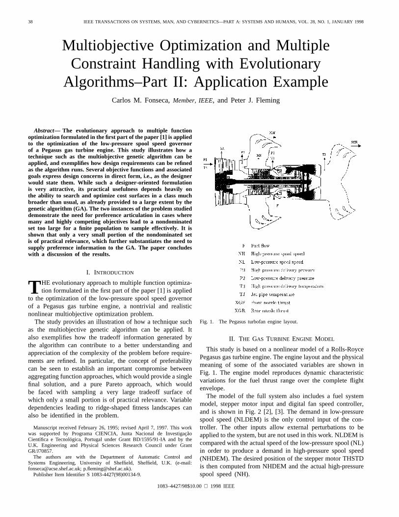
Fig. 1. The Pegasus turbofan engine layout.

II. THE GAS TURBINE ENGINE MODEL

This study is based on a nonlinear model of a Rolls-RoycePegasus gas turbine engine. The engine layout and the physicalmeaning of some of the associated variables are shown inFig. 1. The engine model reproduces dynamic characteristicvariations for the fuel thrust range over the complete flightenvelope.

The model of the full system also includes a fuel systemmodel, stepper motor input and digital fan speed controller,and is shown in Fig. 2 [2], [3]. The demand in low-pressurespool speed (NLDEM) is the only control input of the con-troller. The other inputs allow external perturbations to beapplied to the system, but are not used in this work. NLDEM iscompared with the actual speed of the low-pressure spool (NL)in order to produce a demand in high-pressure spool speed(NHDEM). The desired position of the stepper motor THSTDis then computed from NHDEM and the actual high-pressurespool speed (NH).

1083–4427/98$10.00 1998 IEEE

FONSECA AND FLEMING: EVOLUTIONARY ALGORITHMS—PART II: APPLICATION EXAMPLE 39

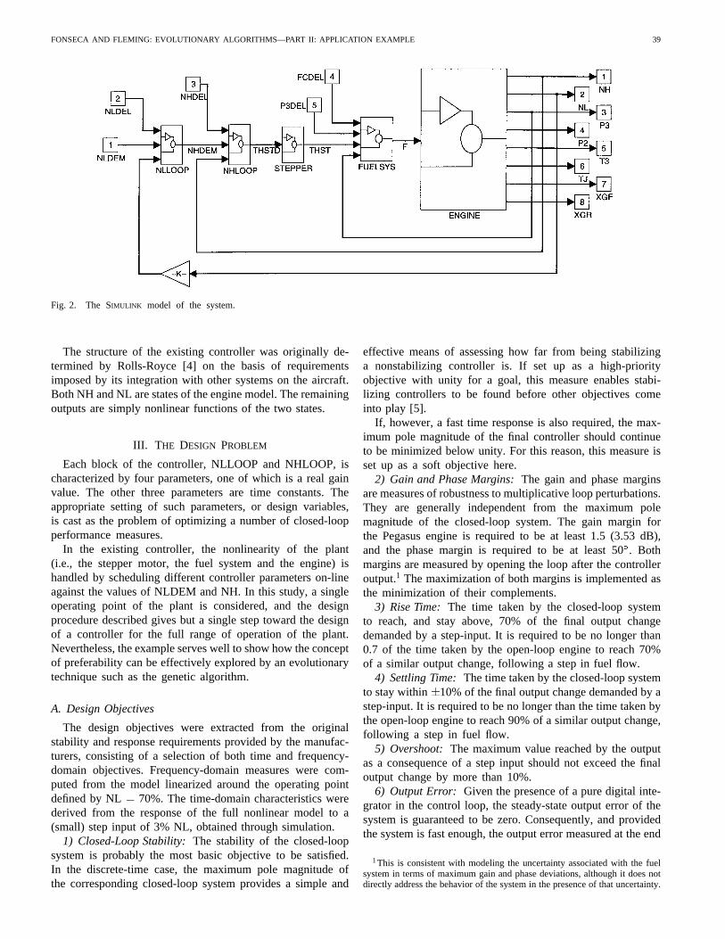
Fig. 2. The SIMULINK model of the system.

The structure of the existing controller was originally de-termined by Rolls-Royce [4] on the basis of requirementsimposed by its integration with other systems on the aircraft.Both NH and NL are states of the engine model. The remainingoutputs are simply nonlinear functions of the two states.

III. T HE DESIGN PROBLEM

Each block of the controller, NLLOOP and NHLOOP, ischaracterized by four parameters, one of which is a real gainvalue. The other three parameters are time constants. Theappropriate setting of such parameters, or design variables,is cast as the problem of optimizing a number of closed-loopperformance measures.

In the existing controller, the nonlinearity of the plant(i.e., the stepper motor, the fuel system and the engine) ishandled by scheduling different controller parameters on-lineagainst the values of NLDEM and NH. In this study, a singleoperating point of the plant is considered, and the designprocedure described gives but a single step toward the designof a controller for the full range of operation of the plant.Nevertheless, the example serves well to show how the conceptof preferability can be effectively explored by an evolutionarytechnique such as the genetic algorithm.

A. Design Objectives

The design objectives were extracted from the originalstability and response requirements provided by the manufac-turers, consisting of a selection of both time and frequency-domain objectives. Frequency-domain measures were com-puted from the model linearized around the operating pointdefined by NL 70%. The time-domain characteristics werederived from the response of the full nonlinear model to a(small) step input of 3% NL, obtained through simulation.

1) Closed-Loop Stability:The stability of the closed-loopsystem is probably the most basic objective to be satisfied.In the discrete-time case, the maximum pole magnitude ofthe corresponding closed-loop system provides a simple and

effective means of assessing how far from being stabilizinga nonstabilizing controller is. If set up as a high-priorityobjective with unity for a goal, this measure enables stabi-lizing controllers to be found before other objectives comeinto play [5].

If, however, a fast time response is also required, the max-imum pole magnitude of the final controller should continueto be minimized below unity. For this reason, this measure isset up as a soft objective here.

2) Gain and Phase Margins:The gain and phase marginsare measures of robustness to multiplicative loop perturbations.They are generally independent from the maximum polemagnitude of the closed-loop system. The gain margin forthe Pegasus engine is required to be at least 1.5 (3.53 dB),and the phase margin is required to be at least 50. Bothmargins are measured by opening the loop after the controlleroutput.1 The maximization of both margins is implemented asthe minimization of their complements.

3) Rise Time:The time taken by the closed-loop systemto reach, and stay above, 70% of the final output changedemanded by a step-input. It is required to be no longer than0.7 of the time taken by the open-loop engine to reach 70%of a similar output change, following a step in fuel flow.

4) Settling Time:The time taken by the closed-loop systemto stay within 10% of the final output change demanded by astep-input. It is required to be no longer than the time taken bythe open-loop engine to reach 90% of a similar output change,following a step in fuel flow.

5) Overshoot: The maximum value reached by the outputas a consequence of a step input should not exceed the finaloutput change by more than 10%.

6) Output Error: Given the presence of a pure digital inte-grator in the control loop, the steady-state output error of thesystem is guaranteed to be zero. Consequently, and providedthe system is fast enough, the output error measured at the end

1This is consistent with modeling the uncertainty associated with the fuelsystem in terms of maximum gain and phase deviations, although it does notdirectly address the behavior of the system in the presence of that uncertainty.


of the simulation should be close to zero. The associated goalis set to 0.1% of the desired output value.2

IV. I MPLEMENTATION

The several objective functions, the multiobjective rankingalgorithm, and all GA routines were implemented as MATLAB

[6] M and MEX-files [7]. A graphical user interface (GUI)was also written as anM-file, making use of the graphicalcapabilities of MATLAB V4. The model was simulated withSIMULINK [8].

A. Parameter Encoding

The controller parameters were encoded as 15-digit binarystrings each, using Gray coding, and then concatenated toform the chromosomes. Gain parameters in the interval [10,10 ), and time constants in the interval [10, 10) (s), werelogarithmically mapped onto the set of possible chromosomevalues, providing a resolution of about foursignificant digits in each case.

B. Genetic Operators

The genetic algorithm consisted of a fairly standard gen-erational GA with multiobjective ranking, and with sharingand mating restriction implemented in the objective domain,as described in Part I [1]. A small percentage (10%) of randomimmigrants was inserted in the population at each generation,with a view to making the GA more responsive to on-linepreference changes [9].

After evaluation, multiobjective ranks were computed ac-cording to the current preferences, and the population sorted.Fitness assignment followed.

1) Fitness Assignment and Selection:The selective pres-sure (defined as the ratio between the number of offspringexpected by the best individual in the population and theaverage number of offspring per individual) imposed by rank-based fitness assignment is constant and can be easily set.In particular, arbitrary values of selective pressure can beobtained by assigning fitness exponentially [10].

In a fixed-size population, the average number of offspringper individual is one and, therefore, the number of offspringexpected by the best individual equals the selective pressure.In the present case, however, only 90% of the individuals inthe new population are the result of selection, the remaining10% consisting of random immigrants. Consequently, for theexpected number of offspring of the best individual to be keptconstant, selective pressure must increase with the percentageof random immigrants introduced in the population. This isuseful in setting parameters such as the mutation rate, asdiscussed below.

By guaranteeing a nonzero, although small, probability ofreproduction to the least fit individuals in the populationfor all values of selective pressure, exponential ranking alsogives random immigrants a chance to take part in the nextrecombination stage of the algorithm. It is desired that, through

2This goal was taken from the steady state stability requirement, whichstates that speed fluctuations should not exceed�0.1% NL.

recombination, they may pass their genetic diversity on tothe population, since it is unlikely that randomly generatedindividuals are able to compete with the current best directlyin terms of fitness, especially as the population evolves towardoptimality.

The fitness assigned to individuals with the same multiob-jective rank is averaged, and fitness shared within each rankbefore selection takes place. The sharing parameter isestimated given the number of preferable individuals in thepresent generation and, for each objective, either the range theydefine in objective space, or the corresponding range definedby the set of preferred individuals found until, and including,the present generation, whichever is smaller. This encouragesthe population to expand across the tradeoff surface, whileallowing it to contract when some of its preferable individualsbecome known to lie outside the preferred region.

Selection uses Baker’s stochastic universal sampling (SUS)algorithm [11], which is optimal in terms of bias and spread. Itminimizes the stochastic errors associated with roulette-wheelselection, and, thus, genetic drift.

2) Recombination:Once the parents of the next generationhave been selected from the old population, they are paired upand recombined with high probability (0.7). Mating restrictionis implemented by forming pairs of individual within a dis-tance of each other in objective space, where possible[12]. Reduced-surrogate [13] shuffle crossover [14] is usedfor recombination.

3) Mutation: Although initially thought to play a secondaryrole in the context of the genetic algorithm [15], mutation hasbeen found to, despite its simplicity, be an important, activesearch operator. Independent bit mutation is characterizedby a single parameter, the bit mutation rate, or probability,the setting of which depends on the selective pressure andchromosome length [16].

If there was no crossover, the probability of an individualnot actually undergoing, or surviving, mutation should be atleast the inverse of the best individual’s expected number ofoffspring for the best individual to, on average, be passedon to the next generation. For lengthchromosomes,

where represents the bit mutation probability. In thepresence of crossover, the actual should be somewherebelow the limit. For , setting

where , was found to perform well. (Note that in thepresence of mating restriction, crossover tends not to be toodestructive.)

C. Offspring Evaluation

Only those offspring which were actually changed by thegenetic operators were reevaluated, as suggested in [17]. Thissimple “caching” mechanism reduced the number of objectivefunction evaluations by between 20% and 25%.


Fig. 3. The cost surface associated with the maximum pole magnitude ofthe closed-loop system.

Fig. 4. The cost surface associated with the phase margin of the closed-loopsystem.

V. RESULTS

The setting of the gain parameters of the controller giventhe existing time-constant parameter values will be consideredfirst. Involving only two decision variables, this formulationmakes it possible to directly visualize cost surfaces in thedecision variable domain.

The optimization of all eight controller parameters follows,with emphasis being put on the articulation of preferences inthe objective domain. The seven objectives described aboveare included in both cases.

A. Two-Variable Example

Consider the problem of minimizing the seven objectivesby varying only the controller gains, KNL and KNH. Sincethere are only two variables, the cost surfaces associated witheach of the objectives can be produced through gridding andvisualized, although this is a computationally intensive task.

Figs. 3–6 depict four of the seven single-objective costsurfaces involved in this problem. Due to the bad scaling ofsome of these objectives, the points on the grid were rankedafter evaluation, as discussed in Part I [1]. Whilst being closerto how a GA with ranking would see them, the resultingsurfaces are much easier to visualize than the original ones.In each case, the axes have been rotated so as to highlight thefeatures of each surface.

It is possible to see how some objectives, notably thosedefined in the time domain, tend to display large flat regions

Fig. 5. The cost surface associated with the settling time of the closed-loopstep response.

Fig. 6. The cost surface associated with the overshoot of the closed-loopstep response.

corresponding either to lowest performance, as with settlingtime (Fig. 5) and rise-time (not shown), or even to optimal per-formance in that objective’s sense, as with overshoot (Fig. 6).However, zero (optimal) overshoot means very little on itsown: for example, it may imply too long a rise-time.

In these regions of the search space, the optimizer mustrely on other objectives, such as the maximum closed-looppole magnitude (Fig. 3). The closed forms used to computethe gain and phase margins, though resulting in fairly fastnumerical algorithms, proved not to be sufficiently numericallyrobust across the whole search space. This is apparent inFig. 4 for the phase margin. Nevertheless, the algorithms didproduce accurate results with “sensible” gain settings, andwere used instead of more stable, but brute-force, approaches.(A discussion of genetic search with approximate functionevaluations can be found in [18].)

One can also estimate and plot a representation of thecost surface associated with the Pareto formulation of theproblem when no goals are specified (Fig. 7). Here, the moststriking features are, perhaps, the large area of the search spacecorresponding to nondominated solutions and the irregularshape of that region, also shown in Fig. 8.

Specifying goals for the objectives defines a much smallerarea of preferable solutions (Figs. 9 and 10), whose dimen-sions approach the resolution of the grid. As it turns out,none of these points is, in fact, satisficing. Actual preferredsolutions, whether satisficing or not, will probably be confinedto an even smaller region of the search space.


Fig. 7. A representation of the cost surface associated with the Pareto-basedformulation in the absence of preference information.

Fig. 8. An alternative view of the nondominated set estimated throughgridding.

1) Genetic Algorithm Results:A genetic algorithm with apopulation size of 100 individuals was run on this problemfive times, each time for 50 generations. Out of a total ofabout 4000 points evaluated in each run, around a half werenondominated relatively to each other. Of these, from ten to200 points were satisficing. Runs in which the populationcould locate itself earlier on the satisficing region rapidlyproduced variations of the first satisficing individuals found,which explains why some runs were apparently much moresuccessful than others.

In this example, some degree of preference informationproves to be absolutely necessary to guide the GA througha very large nondominated set toward solutions of practicalinterest. Fig. 11 illustrates the solutions so-far-preferable atthree different stages of an algorithm run. The preferablesolutions found at the end of the run reveal tradeoffs betweenthe several objectives within the bounds imposed by the goalsassociated with them.

In these plots, objectives are represented by their integerindex on the -axis, and performance in each objectivedimension is plotted on the-axis. Each candidate solution

is represented by a line connecting the points .A tradeoff between adjacent objectives results in the crossingof lines between them, whereas nonconcurrent lines indicatethat those objectives are noncompeting. For example, rise-time

Fig. 9. A representation of the cost surface associated with the formulationincluding goal information.

Fig. 10. An alternative view of the preferable set estimated through gridding.

(objective 4) and settling-time (objective 5) do not seem tocompete heavily. In turn, there is a clear tradeoff betweenthese two objectives and objective 6 (overshoot). The gainand phase margins (objectives 2 and 3) seem to be competingobjectives in part of the tradeoff only.

B. Full Controller Parameter Optimization

The optimization of the full controller assumes no a prioriknowledge of the controller parameter values apart from thatimplicitly used in setting the parameter ranges. Individualsare now 120-bits long, and the population is increased to 150individuals.

Running the GA reveals a much larger set of satisficing solu-tions. The preferable individuals found until, and including, thefortieth generation are shown in Fig. 12(a). When comparedwith the previous example, the solutions found have all greatermaximum pole-magnitudes, that is, longer time-constants. Onthe other hand, they generally exhibit better stability marginsand settling time. Thus, not only do the solutions found inthis second example not dominate those found previously,but also they represent a significantly different region of thepreferable set.

The fact that the eight-variable GA could not find solutionssimilar to, or better than, those found for the two-variableexample shows how sampling the whole preferred region witha population of a given size may not be always feasible,


Fig. 11. Sample tradeoff graphs from a run on the two-variable example, showing the preferable solutions found after ten, 30, and 50 generations. The verticalaxis ranges are the same as those associated with the control-panel sliders. The goal values are given in the middle column of the panel and are plotted as “�”.

even though niche induction mechanisms are used. The di-versity among the preferable individuals in the population atgeneration 40, shown by the corresponding tradeoff graph inFig. 12(b), is an indication that these techniques are indeed atwork, at least to some extent. Nevertheless, their effectivenessin causing the population to spread across the whole, actual,preferred set also depends on the genetic algorithm’s own

ability to capture the regularities in the fitness landscape, andgenerate offspring accordingly. Unfortunately, as discussed inPart I [1], binary coded GA’s cannot be expected to be ableto deal well with strong variable dependencies.

Appropriate interaction with the decision maker can helpaddress this difficulty. The algorithm has found solutionswhich do, in principle, meet their goals, and which it sees all


(a)

(b)

Fig. 12. Sample tradeoff graphs from a run on the eight-variable example, showing preferable solutions found after 40 generations. The vertical axisrangesare the same as those associated with the control-panel sliders. The goal values are given in the middle column of the panel and are plotted as an “�”.(a) Cumulative tradeoff graph after 40 generations. (b) Preferable individuals in the population at generation 40.

as equally fit. Other solutions nonpreferable to these may exist,but they are probably more difficult to find given the encodingstructure used for the chromosomes and the associated geneticoperators. If the DM finds the candidate solutions producedby the GA unacceptable, then preferences should be refinedso as to stimulate the GA to move on to a different region ofthe nondominated set.

As an example, consider again the tradeoff graph inFig. 12(a). The step-response error at the end of thesimulations is not particularly low, reflecting the long timeconstants associated with maximum pole magnitudes close tounity. If faster responses are desired, the DM can tighten thegoals associated with either, or both, of these two objectiveswhile continuing to run the algorithm.

Suppose the DM chooses to lower the goal associated withthe maximum pole magnitude to 0.98. Solutions capable ofmeeting this new requirement turn out not to have yet beenfound, and a set of relatively nondominated solutions close tobeing satisficing is presented to the DM [Fig. 13(a)]. If the DM

believesthis new set of goals can in fact be met (for example,because some goals in the previous set have clearly beenover-attained), there is no algorithmic reason not to specifyit. If the GA cannot find satisficing solutions, it will at leastproduce a set of relatively nondominated approximations tothe new goals on which further preference changes can bebased. As the population continues to evolve, reductions inmaximum pole magnitude are accompanied by reductions inthe step-response error measured at the end of the simulation,and satisficing solutions are eventually found at the expenseof some degradation in gain margin and other objectives[Fig. 13(b)].

Further refinements could involve specifying hard, insteadof soft, bounds for some of the objectives. Suppose the DMdecided that a gain margin of 6 dB seemed possible (inthe presence of the tradeoff graph), and that better gain andphase margins would not be required. Raising the priority ofthese objectives, and changing the gain margin goal, convertsthem into hard constraints as desired. Doing so reduces the


(a)

(b)

Fig. 13. Sample tradeoff graphs showing the effect of tightening one goal’s value. The population is driven toward achieving that goal at the expense ofdegradation with respect to others. (a) After 40 generations (new preferences) and (b) after 60 generations.

preferred set further [Fig. 14(a)], and the process continues.The family of step responses corresponding to the tradeoffgraph in Fig. 14(b) is shown in Fig. 15.

VI. DISCUSSION

In the authors’ search for a reduced, yet illustrative, set ofrealistic design objectives for the Pegasus engine, the ability ofthe GA to exploit omissions in the design requirements soonbecame apparent. The set up of the closed-loop maximum polemagnitude as a soft objective instead of a hard one was a directconsequence of the solutions produced by early runs of thealgorithm being clearly unacceptable: the GA was sometimesable to exploit the nonlinearity of the plant in such a waythat the step-response characteristics achieved were only validfor the particular amplitude of the step used during simulation.Applying slightly larger or smaller steps to the controlled plantimmediately revealed the slow dynamics in the closed loop,deeming the controller unacceptable.

The objective functions and respective goals used in theseexamples reflect design concerns in a direct form. The prob-

lems were formulated from the point of view of the designer,not that of the optimizer. The associated cost landscapes do notall meet common requirements such as continuity, smoothness,and absence of flat regions, and neither does the resultingmultiobjective cost landscape. The practical usefulness of sucha formulation is, therefore, tied to the ability to search andoptimize cost surfaces in a class much broader than usual, asprovided by the GA.

On the other hand, GA’s do work best when no strongdependencies between decision variables exist, which wasneither the case for the simple example given in Part I [1],nor is the case for the Pegasus controller design example.Evolutionary algorithms to be used in multiobjective parameteroptimization should undoubtedly address this issue, because itseems to arise from the very nature of the Pareto formulation.Decision variable dependencies have been taken into accountmainly in the context of evolution strategies [19], at the codinglevel. Simple mating restriction techniques, as described anddiscussed in Part I [1], may require too large a population tobecome effective as the size and complexity of the tradeoff


(a)

(b)

Fig. 14. Sample tradeoff graphs showing the effect of converting two objectives into hard constraints, while also changing the goal associated with ofone of them. (a) After 60 generations (hard stability margins) and (b) after 80 generations.

surfaces increase, while also remaining practical. The prefer-ability relation provides a means of addressing this difficultyby interfacing between the DM and the search algorithm, andallowing the two to interact.

When objective functions are very expensive to evaluate,the interactive use of the MOGA may become less attractivedue to the long time spent at the function evaluation stageof the GA. In such generational EA’s, however, many can-didate solutions can be evaluated independently from eachother, making possible the use of parallelism paradigms whichexploit event replication, while largely avoiding issues such asload balancing and inter-processor communication problems.Parallel formulations (as opposed to parallel implementation)of EA’s are also important alternatives, because of the nichemechanisms which arise in geographically isolated popula-tions.

Finally, evolutionary algorithms are not restricted to pa-rameter optimization. They are also, and probably mainly,powerful combinatoric optimizers. The preferability relationcan, in principle, be applied to virtually all design applications

Fig. 15. Family of preferable step-responses found after 80 generations.

of evolutionary algorithms, whether they involve permutationproblems such as scheduling and the travelling salesman


problem [20], grouping problems such as process-processormapping [21] and nonlinear model term selection [22], or theevolution of computer programs [23].

VII. CONCLUDING REMARKS

The application of the multiobjective genetic algorithm to acontroller design example was used to demonstrate the needfor some degree of preference articulation in Pareto-basedevolutionary optimization. The preferability relation providessuch a mechanism, allowing the designer to concentrate ondesign requirements rather than on the properties of the finalcost function to be optimized.

The interactive use of such an evolutionary multiobjectivealgorithm is very attractive. Speed of execution then becomesan important concern, which can possibly be addressed withparallel processing techniques. The need for improved EA’scapable of addressing strong variable dependencies to someextent has also been highlighted.

ACKNOWLEDGMENT

The authors would like to thank A. Shutler of Rolls-Roycefor sharing his expertise and knowledge in connection withthe Pegasus case-study.

REFERENCES

[1] C. M. Fonseca and P. J. Fleming, “Multiobjective optimization andmultiple constraint handling with evolutionary algorithms–part I: Aunified formulation,” IEEE Trans. Syst., Man, Cybern., this issue, pp.26–37.

[2] S. D. Hancock, “Gas turbine engine controller design using multiobjec-tive optimization techniques,” Ph.D. dissertation, Univ. Wales, Bangor,U.K., 1992.

[3] “Turbofan engine model,” Tech. Rep., Control and CAD Group, Univ.College Swansea, Swansea, U.K., June 1991.

[4] A. G. Shutler, “A case study problem for the advanced controlstechnology club,” Internal Rep. CSAN 2790, Rolls Royce plc, Bristol,U.K., 1991.

[5] C. M. Fonseca and P. J. Fleming, “Multiobjective optimal controllerdesign with genetic algorithms,” inProc. IEE Control’94 Int. Conf.,Warwick, U.K., 1994, vol. 1, pp. 745–749.

[6] MATLAB Reference Guide, The MathWorks, Inc., Aug. 1992.[7] A. Chipperfield, P. Fleming, H. Pohlheim, and C. Fonseca, “Genetic

algorithm toolbox user’s guide,” Res. Rep. 512, Dept. Automatic ControlSyst. Eng., Univ. Sheffield, Sheffield, U.K., July 1994.

[8] SIMULINK User’s Guide, The MathWorks, Inc., Mar. 1992.[9] J. J. Grefenstette, “Genetic algorithms for changing environments,” in

Parallel Problem Solving from Nature 2, R. Mnner and B. Manderick,Eds. Amsterdam, The Netherlands: North-Holland, 1992, pp. 137–144.

[10] P. J. B. Hancock, “An empirical comparison of selection methods inevolutionary algorithms,” inEvolutionary Computing, AISB Workshop,

Terence C. Fogarty, Ed., vol. 865 ofLecture Notes in Computer Science.Berlin, Germany: Springer-Verlag, 1994, pp. 80–94.

[11] J. E. Baker, “Reducing bias and inefficiency in the selection algorithm,”in Genetic Algorithms and Their Applications: Proceedings of the SecondInternational Conference on Genetic Algorithms, J. J. Grefenstette, Ed.Princeton, NJ: Lawrence Erlbaum, 1987, pp. 14–21.

[12] K. Deb and D. E. Goldberg, “An investigation of niche and speciesformation in genetic function optimization,” inProc. 3rd Int. Conf.Genetic Algorithms, J. D. Schaffer, Ed. San Mateo, CA: MorganKaufmann, 1989, pp. 42–50.

[13] L. Booker, “Improving search in genetic algorithms,” inGenetic Al-gorithms and Simulated Annealing, Research Notes in Artificial Intelli-gence, L. Davis, Ed. London, U.K.: Pitman, 1987, ch. 5, pp. 61–73.

[14] R. A. Caruana, L. J. Eshelman, and J. D. Schaffer, “Representation andhidden bias II: Eliminating defining length bias in genetic search viashuffle crossover,” inProc. 11th Int. Joint Conf. Artificial Intelligence,N. S. Sridharan, Ed. San Mateo, CA: Morgan Kaufmann, 1989, pp.750–755.

[15] D. E. Goldberg,Genetic Algorithms in Search, Optimization and Ma-chine Learning. Reading, MA: Addison-Wesley, 1989.

[16] I. Harvey, “Evolutionary robotics and SAGA: The case for hill crawlingand tournament selection,” Cognitive Sci. Res. Paper 222, Univ. Sussex,Brighton, Brighton, U.K., 1992.

[17] P. Oliveira, J. Sequeira, and J. Sentieiro, “Selection of controller parame-ters using genetic algorithms,” inEngineering Systems with Intelligence,S. G. Tzafestas, Ed. Amsterdam, The Netherlands: Kluwer, 1991, pp.431–438.

[18] J. J. Grefenstette and J. M. Fitzpatrick, “Genetic search with approximatefunction evaluations,” inGenetic Algorithms and Their Applications:Proc. 1st Int. Conf. Genetic Algorithms, J. J. Grefenstette, Ed. Prince-ton, NJ: Lawrence Erlbaum, 1985, pp. 112–120.

[19] T. Back, F. Hoffmeister, and H.-P. Schwefel, “A survey of evolutionstrategies,” inGenetic Algorithms: Proc. 4th Int. Conf., R. K. Belew andL. B. Booker, Eds. San Mateo, CA: Morgan Kaufmann, 1991, pp. 2–9.

[20] D. Whitley, T. Starkweather, and D. Shaner, “The travelling salesmanand sequence scheduling: Quality solutions using genetic edge recombi-nation,” in Handbook of Genetic Algorithms, L. Davis, Ed. New York:Van Nostrand Reinhold, 1991, ch. 22, pp. 350–372.

[21] M. J. Baxter, M. O. Tokhi, and P. J. Fleming, “Heterogeneous archi-tectures for real-time control: Design tools and scheduling issues,” inPreprints 12th IFAC Workshop Distributed Computer Control Systems(DCCS’94), J. A. del al Puente and M. G. Rodd, Eds., Toledo, Spain,1994, pp. 89–94.

[22] C. M. Fonseca, E. M. Mendes, P. J. Fleming, and S. A. Billings,“Non-linear model term selection with genetic algorithms,” inIEE/IEEEWorkshop Natural Algorithms Signal Processing, Essex, U.K., 1993, vol.2, pp. 27/1–27/8.

[23] J. R. Koza,Genetic Programming: On the Programming of Computersby Means of Natural Selection. Cambridge, MA: MIT Press, 1992.

Carlos M. Fonseca(S’90–M’95), for a photograph and biography, see thisissue, p. 37.

Peter J. Fleming, for a photograph and biography, see this issue p. 37.

Multiobjective optimization and multiple constraint handling with evolutionary algorithms. II....

Documents

Transcript of Multiobjective optimization and multiple constraint handling with evolutionary algorithms. II....