III European Conference on Computational Mechanics Solids, Structures and Coupled Problems in Engineering

C.A. Mota Soares et.al. (eds.) Lisbon, Portugal, 5–8 June 2006

SEISMIC DESIGN PROCEDURES IN THE FRAMEWORK OF EVOLUTIONARY BASED STRUCTURAL OPTIMIZATION

Manolis Papadrakakis, Nikolaos D. Lagaros, Michalis Fragiadakis

Institute of Structural Analysis & Seismic Research National Technical University of Athens

9, Iroon Polytechniou Str., Zografou Campus, GR-15780 Athens, Greece {mpapadra,nlagaros,mfrag}@central.ntua.gr

Keywords: Seismic design procedures, performance-based design structural optimization, evolutionary algorithms, pushover analysis, nonlinear timehistory analysis.

Abstract. The objective of this paper is twofold: to evaluate seismic design procedures of 3D frame structures and to present a performance-based design procedure for steel structures both in the framework of structural optimization. The evaluation is based on European seis-mic design codes where procedures based on both linear and nonlinear timehistory analysis are adopted. On the other hand the structural performance in the proposed performance-based design procedure is evaluated by means of the reliability demand and resistance meth-odology of U.S. FEMA-350 (Federal Emergency Management Agency) guidelines where the uncertainties and randomness in capacity and seismic demand are taken into account in a consistent manner. The structure has to be able to respond for different hazard levels with a desired confidence. Both Nonlinear Static and Nonlinear Dynamic analysis procedures are used in order to obtain the response at two hazard levels. For the solution of the optimization problems a highly efficient evolutionary algorithm is adopted.

Manolis Papadrakakis, Nikolaos D. Lagaros and Michalis Fragiadakis

2

1 INTRODUCTION

Since the early seventies structural optimization has been the subject of intensive research and several different approaches have been advocated for the optimal design of structures in terms of optimization methods or problem formulation. Most of the attention of the engineer-ing community has been directed towards the optimum design of structures under static load-ing conditions with the assumption of linear elastic structural behaviour. For a large number of real-life structural problems assuming linear response and ignoring the dynamic character-istics of the seismic action during the design phase may lead to structural configurations highly vulnerable to future earthquakes. Furthermore, seismic design codes suggest that under severe earthquake events the structures should be designed to deform inelastically due to the large intensity of the imposed inertia loads.

Performance-Based Design (PBD) has been introduced only recently to increase the safety against natural hazards and, in the case of earthquakes, to make them having a predict-able and reliable performance. In other words, the structures should be able to resist earth-quakes in a quantifiable manner and to preset levels of desired possible damage. Therefore, the modern conceptual approach of seismic structural design is that the structure should meet performance-based objectives for a number of different hazard levels ranging form earth-quakes with a small intensity but also with a small return period to more destructive events with large return periods. The current state of practice in performance-based engineering for steel structures is defined by US guidelines FEMA-350 (Federal Emergency Management Agency) for the design of new buildings and by FEMA-356 for the seismic rehabilitation of existing buildings. These guidelines introduce procedures that can be considered as the first significant diversification from prescriptive building design codes such as EC8 and IBC. Pre-scriptive codes require that the engineer has to ensure that the structure satisfies a number of checks, and in so doing, the structure is supposed to be safe for occupancy. According to a prescriptive code the strength of the structure is evaluated at one loading level corresponding to a single limit state. Serviceability is usually checked as well to ensure that the structure will not deflect or vibrate excessively during its service life.

The structural performance during an earthquake depends highly on a number of uncer-tain parameters. Such parameters are material properties and workmanship or the hysteretic behaviour of the members and the joints. Large randomness also exists in the intensity and the characteristics of earthquake ground motion. Furthermore, uncertainty exists in the analytical procedure that would be adopted and on the mathematical model of the structure. In order to account for as many as possible uncertainties, a reliability-based, performance-oriented ap-proach is proposed by FEMA-350 guidelines. This approach explicitly accounts for uncertain-ties and randomness of seismic demand and capacities in a consistent manner and satisfies the defined reliability performance objectives corresponding to various damage states and seismic hazards. In other words during the optimization process each candidate design must be able to respond with a predefined confidence level.

The objective of this work is to examine the influence of various design procedures adopted by seismic codes on the performance of real-scale structures under an objective framework provided by structural optimization. Several studies have appeared in the literature where seismic design procedures based on non-linear response (e.g. [1,2]) are presented and compared. However, this task can be accomplished in a complete and elaborate manner only in the framework of structural optimization, where the designs obtained with different proce-dures can be directly evaluated by comparing the value of the objective function of the opti-mization problem and the seismic performance of the optimum solution achieved.

Manolis Papadrakakis, Nikolaos D. Lagaros and Michalis Fragiadakis

3

Additionally, it is demonstrated how structural optimization algorithms can be used as a gen-eral-purpose design tool, suitable for very-demanding real-world problems.

Furthermore it is demonstrated how structural optimization can be applied within the reli-ability based framework of FEMA-350 for the design of steel frames, where the demand and re-sistance factor concept is adopted. The proposed methodology is applied using two alterna-tive analytical procedures specified by FEMA-350 as the Nonlinear Static Procedure (NSP) and Nonlinear Dynamic Procure (NDP). In order to handle the increased computational cost of the large number of inelastic time history analyses required by the NDP procedure, parallel processing in a cluster of PCs is performed. In the numerical study presented it is demon-strated how structural optimization can be used to provide more economic designs having bet-ter control on structural performance.

During the last fifteen years there has been a growing interest in optimization algorithms that rely on analogies to natural processes such as Evolutionary Algorithms (EA). For com-plex and realistic structural optimization problems, EA methods appear to be a reliable ap-proach, since most mathematical programming optimizers are prone to converge to a local optimum or may not converge at all. EA do not require the calculation of gradients of the con-straints, as opposed to the widely used in the past mathematical programming algorithms, and thus structural design code checks can be incorporated within an optimization environment as constraints in a straightforward manner.

2 PROGRESS ON SEISMIC DESIGN USING STRUCTURAL OPTIMIZATION PROCEDURES

Structures built according to the provisions of contemporary seismic design codes are de-signed to respond inelastically under strong earthquakes. However, this behaviour is taken into account during the design phase only implicitly. This practice can be mainly attributed to the fact that non-linear timehistory analysis results in increased computational complexity and requires excessive computational resources. In general, a comparatively limited number of studies have been performed for the solution of structural optimization problems under dy-namic loading conditions considering inelastic behaviour. One of the earliest studies on the subject is the work of Polak et al. [4] who minimized the cost of multi-storey frame structures using inelastic timehistory analysis of simplified structural models. Bhatti and Pister [5] and Balling et al. [6] introduced optimization procedures based on nonlinear timehistory analysis. Several limit-states were considered, while different performance objectives are adopted for each limit-state. Pezeshk [7] presented an integrated non-linear analysis and optimal mini-mum weight design methodology, for a simple 3D frame under an equivalent pseudo-static loading scheme.

Following recent developments in structural design procedures [8], a number of research-ers have integrated structural optimization in the framework of Performance-Based Earth-quake Engineering (PBEE). Ganzerli et al. [9] implemented a performance-based optimization procedure of RC frames using convex optimum design models and a standard mathematical optimizer. Esteva et al. [10] presented a performance and reliability-based op-timization under life-cycle considerations using special type damage functions in conjunction with pushover analysis. Gong [11] combined pushover analysis and a dual optimization algo-rithm for the optimal design of steel building frames for various performance levels. Chan and Zou [12] proposed a two-stage, optimality criteria-based, optimization procedure for 2D con-crete frame structures.

The advancements achieved by Evolutionary Algorithms over the past years made possible the solution of real-scale structural optimization problems incorporating design code-based constraints. Two of the earliest studies, where EA were employed for the optimum seismic

Manolis Papadrakakis, Nikolaos D. Lagaros and Michalis Fragiadakis

4

design of structures, are those of Kocer and Arora [13,14] for the optimal design of H-frame transition poles and latticed towers conducting nonlinear timehistory analysis. They proposed the use of Genetic Algorithms (GA) and Simulated Annealing (SA) for the solution of dis-crete variable problems although the computational time required was excessive. Beck et al. [15] proposed a multi-criteria GA-based structural optimisation approach under uncertainties in both structural properties and seismic hazard.

Cheng et al. [16] used a multi-objective GA-based formulation incorporating game and fuzzy set theory for the optimum design of seismically loaded 2D frames. Game theory is used in order to achieve a compromise solution that satisfies all competing objectives in the multi-objective optimization problem, while with the implementation of fuzzy set theory they transformed the constrained optimization problem into an unconstrained one which in turn was solved with a Pareto GA-based optimizer. Liu et al. [17] proposed a GA-based multi-objective structural optimization procedure for steel frames using pushover analysis consider-ing minimum weight, life-cycle cost and design complexity criteria as the objective functions of the optimization problem. The same authors recently extended their methodology in the framework of PBEE [18,19].

As opposed to the aforementioned studies on the optimum seismic design of structures and the different approaches proposed in the past, this work is focused on using structural optimi-zation as a tool for comparing alternative design procedures. The set up of the optimization problem differs according to the design procedure examined, while several issues regarding nonlinear timehistory analysis and structural optimization in the framework of earthquake en-gineering practice are discussed. European seismic design regulations for steel moment resist-ing frames are used as the testbed of the optimum design procedures, while the provisions of U.S. guidelines [20] are also taken into consideration. In total three alternative design proce-dures for seismic design are evaluated in the framework of structural optimization: modal analysis, linear timehistory analysis and nonlinear timehistory analysis. The dynamic analysis based procedures are considered using both natural and artificial ground motion records.

3 SEISMIC DESIGN PROCEDURES

3.1 Analysis methods

According to FEMA-356 [20] four alternative analytical procedures, based on linear and nonlinear structural response, are recommended for the structural analysis of buildings under earthquake loading. The linear procedures can be either the linear static procedure (LSP) or the linear dynamic procedure (LDP). For the linear dynamic procedures there are two alterna-tives, the response spectrum method (which in Eurocode 8 (EC8) [21] is referred as Multi-modal Response Spectrum (MmRS) analysis), and the timehistory method. In a similar fash-ion the nonlinear methods are distinguished to the nonlinear static procedure (NSP), also known as Pushover Analysis, and the nonlinear dynamic procedure (NDP), also referred as inelastic or nonlinear timehistory analysis. Procedures that are not based on dynamic timehis-tory analysis, when applied in the framework of a seismic design code, usually resort to a re-gional response spectrum. Design procedures based on non-linear analysis are less preferred due to their computational cost and the requirements for highly trained engineers to put into practice more elaborate analysis methods. However, when a linear analysis method is em-ployed simplifying assumptions of the structural response are made, resulting either to con-servative and therefore to more expensive designs, or to designs with reduced safety since phenomena that have not been accounted for during the design phase may influence the load carrying capacity of the structure.

Manolis Papadrakakis, Nikolaos D. Lagaros and Michalis Fragiadakis

5

Three different analysis procedures were considered in this study and implemented in the framework of structural optimization. The first corresponds to the EC8 design procedure where the Multi-modal Response Spectrum (MmRS) analysis method is employed. The sec-ond and third correspond to linear elastic and nonlinear inelastic timehistory analysis, respec-tively. Most current design practice is based on the first procedure, while the second is an extension of the first which takes directly into consideration the dynamic characteristics of earthquake loading. The third procedure is considered as the “exact” analysis method requir-ing excessive computational demands.

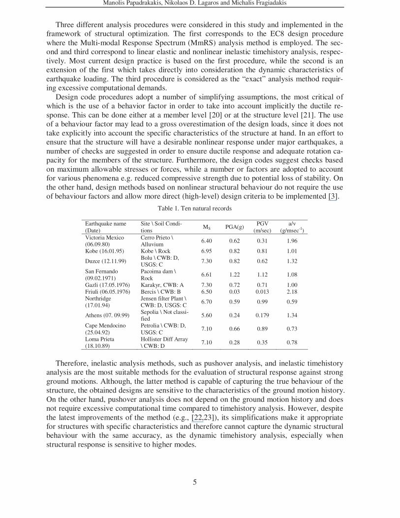
Design code procedures adopt a number of simplifying assumptions, the most critical of which is the use of a behavior factor in order to take into account implicitly the ductile re-sponse. This can be done either at a member level [20] or at the structure level [21]. The use of a behaviour factor may lead to a gross overestimation of the design loads, since it does not take explicitly into account the specific characteristics of the structure at hand. In an effort to ensure that the structure will have a desirable nonlinear response under major earthquakes, a number of checks are suggested in order to ensure ductile response and adequate rotation ca-pacity for the members of the structure. Furthermore, the design codes suggest checks based on maximum allowable stresses or forces, while a number or factors are adopted to account for various phenomena e.g. reduced compressive strength due to potential loss of stability. On the other hand, design methods based on nonlinear structural behaviour do not require the use of behaviour factors and allow more direct (high-level) design criteria to be implemented [3].

Table 1. Ten natural records

Earthquake name (Date)

Site \ Soil Condi-tions

MS PGA(g) PGV (m/sec)

a/v

(g/msec-1) Victoria Mexico (06.09.80)

Cerro Prieto \ Alluvium

6.40 0.62 0.31 1.96

Kobe (16.01.95) Kobe \ Rock 6.95 0.82 0.81 1.01

Duzce (12.11.99) Bolu \ CWB: D, USGS: C

7.30 0.82 0.62 1.32

San Fernando (09.02.1971)

Pacoima dam \ Rock

6.61 1.22 1.12 1.08

Gazli (17.05.1976) Karakyr, CWB: A 7.30 0.72 0.71 1.00 Friuli (06.05.1976) Bercis \ CWB: B 6.50 0.03 0.013 2.18 Northridge (17.01.94)

Jensen filter Plant \ CWB: D, USGS: C

6.70 0.59 0.99 0.59

Athens (07. 09.99) Sepolia \ Not classi-fied

5.60 0.24 0.179 1.34

Cape Mendocino (25.04.92)

Petrolia \ CWB: D, USGS: C

7.10 0.66 0.89 0.73

Loma Prieta (18.10.89)

Hollister Diff Array \ CWB: D

7.10 0.28 0.35 0.78

Therefore, inelastic analysis methods, such as pushover analysis, and inelastic timehistory

analysis are the most suitable methods for the evaluation of structural response against strong ground motions. Although, the latter method is capable of capturing the true behaviour of the structure, the obtained designs are sensitive to the characteristics of the ground motion history. On the other hand, pushover analysis does not depend on the ground motion history and does not require excessive computational time compared to timehistory analysis. However, despite the latest improvements of the method (e.g., [22,23]), its simplifications make it appropriate for structures with specific characteristics and therefore cannot capture the dynamic structural behaviour with the same accuracy, as the dynamic timehistory analysis, especially when structural response is sensitive to higher modes.

Manolis Papadrakakis, Nikolaos D. Lagaros and Michalis Fragiadakis

6

3.2 Earthquake loading

In the present study, each candidate design is checked against the provisions of EC3 [24] and EC8 [21] during the optimization process. Two design load combinations are considered:

d kj kij i

S 1.35 G " "1.50 Q= +∑ ∑ (1)

d kj d 2i kij i

S G " "E " " Q= + + ψ∑ ∑ (2)

where “+” implies “to be combined with”, the summation symbol “Σ” implies “the combined effect of”, Gkj denotes the characteristic value “k” of the permanent action j, Ed is the design value of the seismic action, and Qki refers to the characteristic value “k” of the variable action i, while ψ2i is the combination coefficient for quasi permanent value of the variable action i, here taken equal to 0.30. Furthermore, for 3D problems earthquake actions must be consid-ered using the following combinations:

d dx dy

d dx dy

E E 0.30E

E 0.30E E

= +

= + (3)

where Edx and Edy represent earthquake loading at two perpendicular to each other directions. When natural records are used they must consist of two perpendicular components from the same earthquake. All design code checks are implemented into the optimization problem as constraints.

The design procedures adopted in the present investigation differ in the way they take into account earthquake loading. The first procedure is based on the EC8 response spectrum, while the two timehistory procedures are based on suites of natural or artificial earthquake records. The selection of the proper seismic loading for design purposes is not an easy task due to the inherent uncertainties in seismic loading. For this reason a more rigorous treatment of seismic loading is to assume that the structure is subjected to a set of natural or artificial records that match the characteristics of the site where the structure is to be located. The dynamic analysis procedures in current U.S. seismic design provisions and guidelines specify that a series of non-linear timehistory analyses are conducted with pairs of horizontal ground motion compo-nents selected from not less than three seismic events. If three pairs of records are used, then the maximum value of the response parameter of interest (e.g., peak lateral displacement) is used for the evaluation of the current design, while if seven or more pairs of records are used, then the median value of the response parameter may be used. However, these are minimum requirements and in practice it is advised to use a larger number of records, e.g. 10 or more, since the seismic response is very sensitive to the choice of records. Moreover, the use of the median response is preferable compared to the mean, since the median is not sensitive to out-liers and its value is not affected when the structure collapses under some records.

In order to determine the damaging potential of each record a classification is performed according to the peak ground acceleration (PGA) to peak ground velocity (PGV), the so-called a/v ratio [25]. This ratio reflects many source characteristics, travel path and site condi-tions, as well as, structural response parameters. With regard to structural response, high a/v ratios will be more critical for stiffer, short period structures, while more flexible, long period structures will be strongly shaken by earthquakes with low a/v ratios. These ranges approxi-mately can be determined as:

Manolis Papadrakakis, Nikolaos D. Lagaros and Michalis Fragiadakis

7

-1 -1

-1

-1

0.8g/ms / 1.2g/ms (Normal)

1.2g/ms / (High)

/ 0.8g/ms (Low)

a v

a v

a v

≤ ≤

<

<

(4)

where: Normal (a/v) refers to ground motions time histories with significant energy content for a broad range of frequencies. High (a/v) refers to ground motions with many large-amplitude, high-frequency oscillations. Low (a/v) refers to ground motions in which the sig-nificant response is contained in a few long duration acceleration pulses.

In the present study the ground motion records listed in Table 1 were used, where PGA and PGV values refer to the stronger, in terms of PGA, of the two horizontal components of each record. These records cover a sufficient range of a/v ratios. Figure 1 shows the 2.5%-damped EC8 elastic response spectrum and the corresponding spectra of the records of Table 1. Scal-ing the ground motion records is necessary in order to make all records compatible with the design spectrum of EC8. Among the many ways of scaling ground motion records, a widely accepted choice is the 5%-damped first mode spectral acceleration. Shome et al. (1998) [26] found that when using this scaling approach the bias of damage estimation is not statistically significant.

0 0.5 1 1.5 2 2.5 3 3.5 40

0.5

1

1.5

2

2.5

3

T (sec)

Sa

(g)

Figure 1: EC8 2% damped spectrum and scaled spectra of Table 1 records

However, in cases where the participation of higher modes has significant impact on the structural response, a scale factor that covers a wide range of modes should be used. In this investigation each record is scaled by a factor that minimizes the error with respect to the EC8 spectrum at a number of NT structural periods (typically from 0.1 to 4 seconds). Thus, the scaling factor λ is computed as follows:

8

1

( )min 1

( )

T recordNa i

ECi a i

S Terror

S T=

⎛ ⎞⎛ ⎞λ ⋅= −⎜ ⎟⎜ ⎟⎜ ⎟⎝ ⎠⎝ ⎠

∑ (5)

where 8( )ECa iS T , ( )record

a iS T are the spectral accelerations for the ith period value from the EC8 and the record response spectrum, respectively.

Apart from enriching the catalogues of earthquake records of a region, a second reason for using artificial records is that they usually present a larger number of cycles than natural re-

Manolis Papadrakakis, Nikolaos D. Lagaros and Michalis Fragiadakis

8

cords and therefore they result to more severe earthquake loading for a greater range of struc-tural periods. Although one may argue that artificial records are unrealistic and thus they do not simulate an earthquake, they can still be considered as an envelope ground motion and hence as a more conservative loading scenario. Five uncorrelated artificial accelerograms, produced from the smooth EC8 spectrum are used in the present study. The methodology adopted for the creation of artificial accelerograms from a given smooth spectrum was pro-posed by Gasparini and Vanmarke [27]. A typical artificial accelerogram and its correspond-ing 2.5%-damped spectrum are shown in Figure 2. Scaling is not required in the case of artificial records since they represent the same earthquake hazard with the smooth spectrum they were generated from.

0 5 10 15 20−0.4

−0.3

−0.2

−0.1

0

0.1

0.2

0.3

0.4

Time (sec)

Acc

eler

atio

n (g

)

(a)

0 0.5 1 1.5 2 2.5 3 3.5 40

0.2

0.4

0.6

0.8

1

1.2

1.4

1.6

1.8

2

T (sec)

Sa

(g)

(b)

Figure 2: (a) A typical artificial accelerogram, (b) 2.5% damped response spectra of EC8 and of the artificial accelerogram of Figure 2(a)

3.3 Finite element modeling

In order to perform dynamic analysis considering inelastic behaviour there is a need for a detailed and accurate simulation of the structure in the areas where plastic deformations are expected to occur. Given that the plastic hinge approach has limitations in terms of accuracy, especially under dynamic loading, the fiber approach was adopted in this study. A fiber beam element based on the natural mode method has been employed [28]. This finite element for-mulation is based on the natural mode method where the description of the displacement field along the beam is performed with quantities having a clear physical meaning.

Each structural element is discretized into a number of sections, and each section is further divided into a number of fibers (Figure 3), which are restrained to beam kinematics. The sec-tions are located either at the centre of the element or at its Gaussian integration points. The

Manolis Papadrakakis, Nikolaos D. Lagaros and Michalis Fragiadakis

9

main advantage of the fiber approach is that each fiber has a simple uniaxial material model allowing an easy and efficient implementation of the inelastic behaviour. This approach is considered suitable for inelastic beam-column elements under dynamic loading and provides reliable solution compared to other formulations for inelastic analysis of frame structures.

zifib

yifib

y

z

x

L

b

h

Aifib,Eifib

(a)

zifib

yifib

y

z

Aifib,Eifib

(b)

Figure 3. Modelling of inelastic behaviour-The fiber approach

However, it results to higher computational demands both in terms of memory storage and CPU time. An adaptive discretization is used where a detailed simulation is restricted to the regions of the joints. Thus, the vicinity (usually 2.5% to 10% of element’s length) of beam and column joints is discretized with a denser mesh of beam elements, while the remaining part of the member is discretized with linear elastic elements.

A simple bilinear stress-strain relationship with kinematic hardening is adopted. Studies have shown that this law is adequate and gives accurate results for many practical applications. The stress-strain relationship that allows for strain hardening is:

( )

y

y st y y

σ , for

σ , for

= Ε ⋅ε ε ≤ ε

= Ε ⋅ε + Ε ⋅ ε − ε ε > ε (6)

where σy and εy are the yield strain and the corresponding yield stress, E is the elastic Young’s modulus and Est is the strain-hardening modulus. 4 PERFORMANCE-BASED DESIGN OPTIMIZATION

Prescriptive building codes cannot provide acceptable levels of building life-cycle perform-ance because they include a great number of provisions designed to ensure adequate strength of structural members and, indirectly or implicitly, of the overall structural strength. The basic philosophy of a PBD procedure is to allow engineers to determine explicitly the seismic de-mands at preset performance levels by introducing design checks of a higher level.

4.1 Performance Levels and Objectives

Building performance is a combination of the performance of both structural and nonstruc-tural components. FEMA-350 describes the overall levels of structural and nonstructural damage that buildings are expected to meet using two performance levels, the Collapse Pre-

Manolis Papadrakakis, Nikolaos D. Lagaros and Michalis Fragiadakis

10

vention (CP) level and Immediate Occupancy (IO) level. The CP performance level corre-sponds to a hazard level with a 2% probability of exceedance in 50 years (2/50) and is defined as the post earthquake damage state in which the structure is on the verge of experiencing par-tial or total collapse. Substantial damage to the structure has occurred, potentially including significant degradation in the stiffness and strength of the lateral-force-resisting system and large permanent lateral deformation of the structure. The IO performance level corresponds to a hazard level with a 50% probability of exceedance in 50 years (50/50) and is defined as the post earthquake damage state in which only limited structural damage has occurred. Damage is anticipated to be so slight that no repair is required after the earthquake. Buildings that meet this performance level should be safe for immediate post earthquake occupancy. FEMA-350 guidelines provide the framework for the estimation of the level of confi-dence that a structure will be able to achieve a desired performance objective. The main dif-ference with the FEMA-356 guidelines is that the performance objectives are not expressed in a deterministic manner. Each performance objective set by FEMA-350 guidelines consist of a hazard level, for which the corresponding performance is to be achieved. For example, a de-sign may be determined to provide at least a 90% level of confidence of the performance ob-jective for the CP, for earthquake hazards with a 2% probability of exceedance in 50 years, and with a 50% or higher level of confidence for IO, for earthquake hazards with a 50% prob-ability of exceedance in 50 years. The confidence levels are obtained by means of the factored demand to capacity ratio where a number of parameters are considered that introduce explic-itly the uncertainty in prediction of seismic demand and in the analytical procedure adopted as well as the uncertainty and randomness in the prediction of structural capacity.

4.2 Acceptance Criteria - Optimization Constraints

A number of constraints must be expressed for the structural optimization problem in order the optimum design to be acceptable in practice. FEMA-350 and EC3 provisions are adopted in order to formulate these constraints. Each candidate design is verified against these con-straints, while care should be taken during the optimization process in order to perform the checks that require less computational effort first. Therefore, prior to any analysis the column to beam strength ratio is calculated and also a check is performed on whether the sections chosen are of class 1, as EC3 suggests. The later check is necessary in order to ensure that the members have the capacity to develop their full plastic moment and rotational ductility, while the former is necessary in order to have a design consistent with the ‘strong column-weak beam’ design philosophy. Subsequently, all EC3 checks must be satisfied for the gravity loads using the following load combination of Eq. (1).

If the above constraints are satisfied, then nonlinear static or dynamic analysis is per-formed for both hazard levels for the selected ground motion records. When the dynamic analysis procedure is adopted, the maximum interstorey drift value or the median drift value is obtained depending on the number of records used. According to FEMA standards, if less than seven records are used the maximum drift value must be considered, otherwise the me-dian value must be used instead. For the analysis step, for both analytical procedures earth-quake loading is applied using the following load combination of Eq. (2).

Acceptability of the structural performance is evaluated using the FEMA-350 procedure where the level of confidence that the building has the ability to meet the desired performance objectives is determined. The confidence level is determined through evaluation of the fac-tored-demand-to-capacity ratio which is given by the expression:

Manolis Papadrakakis, Nikolaos D. Lagaros and Michalis Fragiadakis

11

D

Cαγ ⋅ γ ⋅

λ =φ⋅ (7)

where: C is the median estimate of the capacity of the structure, expressed as the maximum intersto-

rey drift demand. D is the calculated demand for the structure, can be obtained either from nonlinear static or

nonlinear dynamic analysis. γ is the demand variability factor that accounts for the variability inherent in the prediction of

demand related to assumptions made in structural modelling and prediction of the character of ground motion.

γα is the analysis uncertainty factor that accounts for bias and uncertainty, associated with the specific analytical procedure used to estimate demand as a function of ground shaking in-tensity.

φ is the resistance factor that accounts for the uncertainty and variability inherent in the pre-diction of structural capacity as a function of ground shaking intensity.

Detailed description and the theoretical background of these parameters are provided by FEMA-350 (Appendix A). In the present study the above parameters take values from FEMA-350 tables. Table 2 lists the values adopted in this study for mid-rise moment frames with rigid connections for both nonlinear static and nonlinear dynamic analysis.

Table 2. Parameters for the Evaluation of Confidence for mid-rise Special Moment frames according to FEMA-350

IO Performance Level CP Performance Level NSP NDP NSP NDP

βUT 0.20 0.20 0.40 0.40 C 0.02 0.02 0.10 0.10

φ 1.00 1.00 0.85 0.85

γ 1.40 1.40 1.20 1.20

aγ 1.45 1.02 0.99 1.06

Once λ of Eq. (7) is known, the following expression is solved for KΧ :

{ }exp -bβ ( β / 2)UT X UTK kλ = − (8)

where: KX is the standard Gaussian variate associated with probability x of not being exceeded found

in standard probability tables. b is a coefficient relating the incremental change in demand to an incremental change in

ground shaking intensity, at the hazard level of interest, typically taken as having a value of 1.0

βUT is an uncertainty measure coefficient dependent on a number of sources of uncertainty in the estimation of structural demands and capacities. Sources of uncertainty include, for ex-ample, the actual material properties, effective damping and other. If the uncertainty asso-ciated with each source i is denoted asβUi , then βUT is obtained as:

β β2

UT Uii= ∑ (9)

Manolis Papadrakakis, Nikolaos D. Lagaros and Michalis Fragiadakis

12

k is the slope of the hazard curve when plotted on a log-log scale, where the hazard curve is of the form:

( ) 0k

Si i iH S k S −= (10)

where: ( )Si iH S is the probability of ground shaking having spectral response acceleration greater

than Si and k0 is a constant that depends on the seismicity of the site. The confidence level for each performance objective is obtained once the factored demand to capacity ratio (Eq. (7)) is computed and Eq. (8) is solved for KΧ. The confidence level for each performance level can be easily obtained from conventional probability tables. For example, if KΧ is 1.28 the confidence level is 90%. According to FEMA-350 when the global behaviour is limited by interstorey drift, the minimum confidence levels are 90% for the CP and 50% for the IO level. In order to implement the above procedure in a structural optimization environ-ment the factored demand to capacity ratio is obtained for each performance level and a con-straint in the maximum interstorey drift is formulated by rearranging Eq. (7):

0

a

CD

λ ⋅φ⋅− ≤

γ ⋅ γ (11)

5 FORMULATION OF THE STRUCTURAL OPTIMIZATION PROBLEM

In sizing optimization problems usually the aim is to minimize the weight of the structure under certain behavioral constraints on stress and displacements. The design variables are most frequently chosen to be dimensions of the cross-sectional areas of the members of the structure. Due to engineering practice demands the members are divided into groups having the same design variables. This linking of elements results in a trade-off between the use of more material and the need of symmetry and uniformity of structures due to practical consid-erations. Furthermore, due to fabrication limitations the design variables are not continuous but discrete. A discrete structural optimization problem can be formulated in the following form:

j

i

min F(s)

subject to g (s) 0 j=1,...,m

s , i=1,...,ndR

≤

∈ (12)

where Rd is a given set of discrete values and the design variables si (i=1,...,n) can take values only from this set.

5.1 Solving the optimization problem with Evolution Strategies

The sensitivity analysis phase, which is an important ingredient of all mathematical pro-gramming optimization methods, is the most time-consuming part of the optimization process when a gradient-based optimizer is used [29]. On the other hand, the application of random search optimization methods, such as evolutionary algorithms, do not need gradient informa-tion and therefore avoid performing the computationally expensive sensitivity analysis step [30,31]. Furthermore, it is widely recognized that evolution-based optimization techniques are in general more robust and present a better global behavior than mathematical programming methods. Moreover, the feasible design space in structural optimization problems under dy-

Manolis Papadrakakis, Nikolaos D. Lagaros and Michalis Fragiadakis

13

namic constraints is often disconnected or disjoint which causes difficulties for many conven-tional optimization algorithm. They may suffer, however, from a slow rate of convergence towards the global optimum.

In the current study Evolution Strategies (ES) have been employed for the solution of the optimization problem. ES imitate biological evolution in nature and have three characteristics that make them differ from other conventional optimization algorithms: (i) in place of the usual deterministic operators, they use randomized operators: mutation, selection as well as recombination; (ii) instead of a single design point, they work simultaneously with a popula-tion of design points in the space of variables; (iii) they can handle continuous, discrete and mixed optimization problems. The second characteristic allows for a natural implementation of ES on parallel computing environments. The ES was initially applied for continuous opti-mization problems, but they have also been implemented in discrete and mixed optimization problems.

In engineering practice the design variables are not continuous because usually the struc-tural parts are constructed with certain variation of their dimensions. Thus design variables can only take values from a predefined discrete set. For the solution of discrete optimization problems, as the ones considered in the present study, a modified ES algorithm can be used. The basic differences between discrete and continuous ES are focused on the mutation and the recombination operators. The multi-membered ES (M-ES), adopted in the current study, use the three standard genetic operators: recombination, mutation and selection.

The ES optimization procedure starts with a set of parent vectors. If any of these parent vectors gives an infeasible design then this parent vector is modified until it becomes feasible. Subsequently, the offsprings are generated and checked if they are in the feasible region. Ac-cording to (μ+λ) selection scheme in every generation the values of the objective function of the parent and the offspring vectors are compared and the worst vectors are rejected, while the remaining ones are considered to be the parent vectors of the new generation. On the other hand, according to (μ,λ) selection scheme only the offspring vectors of each generation are used to produce the new generation. This procedure is repeated until the chosen termination criterion is satisfied. The number of parents and offsprings involved affects the computational efficiency of the multi-membered ES. It has been observed that when the values of μ and λ are taken equal to the number of the design variables produce better results.

The ES algorithm for structural optimization applications under seismic loading can be stated as follows: 1. Selection step: selection of si (i = 1,2,...,μ) parent vectors of the design variables. 2. Structural analysis step 3. Constraints check: all parent vectors become feasible. 4. Offspring generation: generate sj, (j=1,2,...,λ) offspring vectors of the design variables. 5. Structural analysis step 6. Constraints check: if satisfied continue, else change sj and go to step 4. 7. Selection step: selection of the next generation parents. 8. Convergence check: If satisfied stop, else go to step 4.

5.2 Optimum seismic design procedures and constraints

Regardless the analysis procedure adopted, there is a number of behavioural constraints that have to be taken into consideration in order to ensure that during the optimization proce-dure the structure fulfils design code requirements. For example, FEMA-356 makes a clear distinction between deformation-based and force-based actions and specifies separate per-formance criteria for each type of action. For structural optimization problems under earth-quake loading the constraints adopted are derived from seismic performance criteria specified

Manolis Papadrakakis, Nikolaos D. Lagaros and Michalis Fragiadakis

14

by structural codes or guidelines. These criteria are placed into categories according to the analysis procedure, linear or nonlinear, used for the design. The criteria are further classified according to the performance level they refer to. In the present study a single performance level is adopted, namely Life Safety, due to the increased computational cost to perform struc-tural optimization for a wider range of performance levels.

In both linear and nonlinear procedures, before proceeding to the analysis part at each op-timization step, the strength ratio of column to beam is calculated and a check whether the sections chosen are of class 1, as EC3 suggests, is carried out. The later check is necessary in order to ensure that the members have the capacity to develop their full plastic moment and rotational ductility, while the check on the ratio of the column strength over the strength of the beam is necessary in order to have designs consistent with the ‘strong column-weak beam’ philosophy. Subsequently, linear or nonlinear analysis is carried out and a number of design checks are performed.

5.3 Constraints for Linear Analysis Procedures

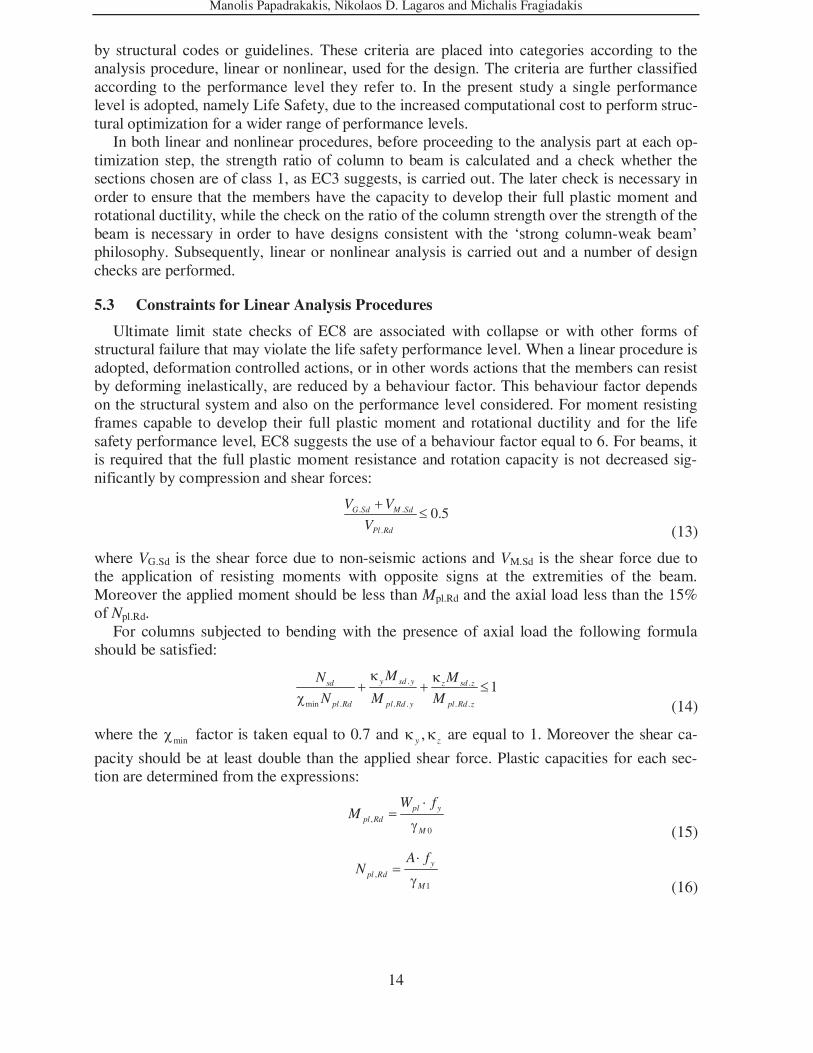
Ultimate limit state checks of EC8 are associated with collapse or with other forms of structural failure that may violate the life safety performance level. When a linear procedure is adopted, deformation controlled actions, or in other words actions that the members can resist by deforming inelastically, are reduced by a behaviour factor. This behaviour factor depends on the structural system and also on the performance level considered. For moment resisting frames capable to develop their full plastic moment and rotational ductility and for the life safety performance level, EC8 suggests the use of a behaviour factor equal to 6. For beams, it is required that the full plastic moment resistance and rotation capacity is not decreased sig-nificantly by compression and shear forces:

. .

.

0.5G Sd M Sd

Pl Rd

V V

V

+≤

(13)

where VG.Sd is the shear force due to non-seismic actions and VM.Sd is the shear force due to the application of resisting moments with opposite signs at the extremities of the beam. Moreover the applied moment should be less than Mpl.Rd and the axial load less than the 15% of Npl.Rd.

For columns subjected to bending with the presence of axial load the following formula should be satisfied:

. .

min . . . . .

1y sd ysd z sd z

pl Rd pl Rd y pl Rd z

MN M

N M M

κ κ+ + ≤

χ (14)

where the minχ factor is taken equal to 0.7 and ,κ κy z are equal to 1. Moreover the shear ca-

pacity should be at least double than the applied shear force. Plastic capacities for each sec-tion are determined from the expressions:

,

0

pl ypl Rd

M

W fM

⋅=

γ (15)

,

1

ypl Rd

M

A fN

⋅=

γ (16)

Manolis Papadrakakis, Nikolaos D. Lagaros and Michalis Fragiadakis

15

,

0

1.04

3w y

pl Rd

M

h t fV

⋅ ⋅ ⋅=

⋅ γ (17)

where parameters M0γ and M1γ are taken both equal to 1.10. The stress check of equation (14) is performed for both the weak and the strong axis of the member when biaxial actions are present. The stability coefficient θ is evaluated for each storey using the formula:

tot r

tot

P d

V h

⋅θ =

⋅ (18)

where Ptot is the total gravity load at the storey considered, dr is the interstorey drift, Vtot is the total seismic shear and h is the storey height. P-Δ effects need not be considered when the stability coefficient is less than 0.1.

5.4 Constraints for Nonlinear Analysis Procedures

The use of nonlinear analysis procedures allows more direct performance criteria to be adopted. Performance criteria that refer to the local member level, such as plastic hinge rota-tions or member chord rotations can be used. Alternatively, storey level criteria, such as maximum interstorey drift values, can also be adopted. Suggested values for plastic hinge ro-tations and maximum interstorey drift values are given for steel moment resisting frames by FEMA-356 and FEMA-350. Since nonlinear analysis is performed the P-Δ effects can be taken into account explicitly. In the present study, a maximum interstorey drift value of 2% is considered for the Life Safety performance level.

Furthermore, another restriction is that the applied axial force on columns should not ex-ceed 50% of the member capacity given by Eq. (16), in order to allow ductile structural be-haviour. If the nonlinear dynamic analysis fails to converge it is considered that the structure has lost its stability during the ground motion, and thus the design is rejected. 6 NUMERICAL RESULTS

6.1 Assessment of the design procedures

The six storey space frame, shown in Figure 4, has been considered for the purpose of the current study. The space frame consists of 63 members, simulated with 383 beam elements (6 adaptively distributed beam-column elements per member and approximately 100 fibers in each member) and about 2100 d.o.f. The modulus of elasticity is 200 GPa and the yield stress is fy=250 MPa. The structural members are divided into five groups, each of them having one design variable, i.e. element’s cross-section, thus corresponding to 5 independent design vari-ables. All sections are W-shaped given by standard AISC tables.

Manolis Papadrakakis, Nikolaos D. Lagaros and Michalis Fragiadakis

16

Figure 4. Six storey space frame

1

2

3

4

5

6

0 0.005 0.01 0.015 0.02 0.025 0.03

Maximum Interstorey Drift Ratio (θ max)

Sto

rey

MmRSLDP - NATLDP - ARNDP - NATNDP - AR

7

Figure 5. Seismic performance of the five optimum designs: Profiles of median maximum interstorey drifts

The structure is loaded with G=3kPa permanent action and a live load of Q=5 kPa in the vertical direction. Earthquake loading is taken into account using the EC8 response spectrum (Figure 1) for a PGA value of 0.40g. Both LDP and NDP design procedures are considered with either a suite of 10 natural records, scaled to the EC8 response spectrum according to Eq. (5), or 5 artificial accelerograms generated from the same spectrum. For all linear procedures, including the MmRS procedure, the design spectrum is reduced by a behaviour factor q=6.0 as suggested by EC8 for steel moment resisting frame structures.

All the optimization analyses in this study were performed with a ES(5+5) scheme, while the same initial feasible population was employed for all cases examined. The objective func-tion of the optimization problem is the structural weight. In total five cases were examined; the MmRS procedure using the EC8 spectrum, and the LDP and the NDP using either 10

Manolis Papadrakakis, Nikolaos D. Lagaros and Michalis Fragiadakis

17

natural records (cases LDP-NAT and NDP-NAT) or 5 artificial records (cases LDP-AR and NDP-AR).

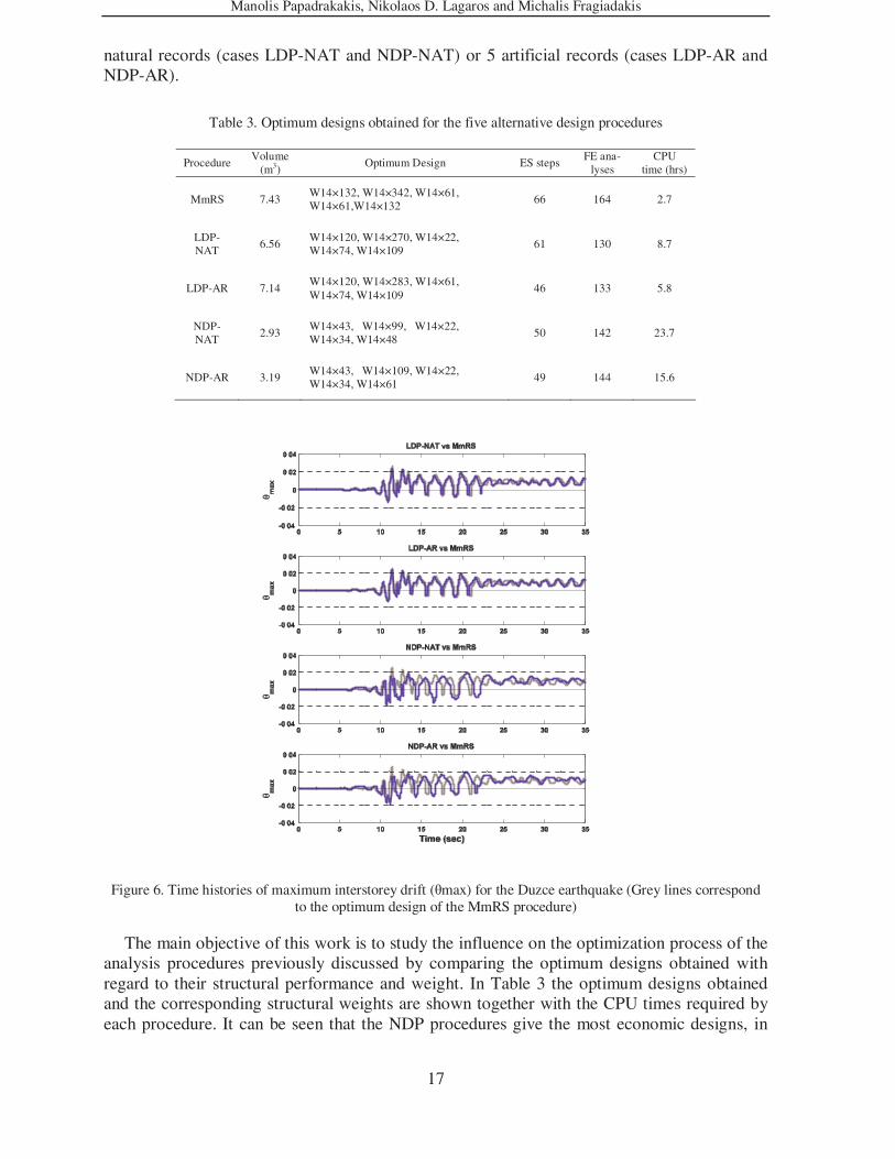
Table 3. Optimum designs obtained for the five alternative design procedures

Procedure Volume

(m3) Optimum Design ES steps

FE ana-lyses

CPU time (hrs)

MmRS 7.43 W14×132, W14×342, W14×61, W14×61,W14×132

66 164 2.7

LDP-NAT

6.56 W14×120, W14×270, W14×22, W14×74, W14×109

61 130 8.7

LDP-AR 7.14 W14×120, W14×283, W14×61, W14×74, W14×109

46 133 5.8

NDP-NAT

2.93 W14×43, W14×99, W14×22, W14×34, W14×48

50 142 23.7

NDP-AR 3.19 W14×43, W14×109, W14×22, W14×34, W14×61

49 144 15.6

Figure 6. Time histories of maximum interstorey drift (θmax) for the Duzce earthquake (Grey lines correspond to the optimum design of the MmRS procedure)

The main objective of this work is to study the influence on the optimization process of the analysis procedures previously discussed by comparing the optimum designs obtained with regard to their structural performance and weight. In Table 3 the optimum designs obtained and the corresponding structural weights are shown together with the CPU times required by each procedure. It can be seen that the NDP procedures give the most economic designs, in

Manolis Papadrakakis, Nikolaos D. Lagaros and Michalis Fragiadakis

18

terms of the material weight, while the MmRS procedure lead to the most expensive solution. Furthermore, comparing the dynamic procedures with natural and artificial records it can be seen that natural records lead to less material weight. The LDP procedures compared to the MmRS procedure achieved a structural weight reduction of 12% and 4% for the natural re-cords (NAT) and the artificial records (AR) case, respectively, while the corresponding reduc-tion of the NDP procedures is 60% and 57%, respectively. Furthermore, it can be seen that the number of ES optimization steps and the number of FE analyses required are reasonable for such complicated, non-convex, problems.

In Figure 5 the seismic performance of the five optimum designs is compared in terms of their profiles of maximum interstorey drifts. More specifically, Figure 5 shows the median of the maximum interstorey drift values for each of the five optimum designs along the height of the frame when nonlinear timehistory analysis is performed using the records of Table 1. From Table 3 and Figure 5 it can be seen that even though the MmRS procedure leads to the most conservative design in terms of structural weight achieved (7.43m3), it results to the highest interstorey drift values compared to the remaining four optimum designs. Similarly the optimum designs of the LDP procedure exhibit interstorey drift values slightly larger than the 2% drift limit imposed on the NDP designs but in terms of material weight the LDP de-signs are considerably heavier. This is attributed to the nature of the constraints imposed on the linear procedures, as opposed to the direct design criteria adopted in the nonlinear analysis procedures as it is described in section 4.2. The designs obtained with artificial records both for the LDP and the NDP procedures resulted in slightly heavier designs with approximately the same maximum interstorey drift values. This can be partially explained by the large num-ber of significant cycles that artificial records contain and thus they pose a more conservative loading scheme.

Similar conclusions arise from Figure 6 where the optimum designs of the dynamic proce-dures are compared against the optimum design of the MmRS procedure, when subjected to the Duzce earthquake. It can be seen that the optimization procedure is dominated by two or three cycles, where the maximum interstorey drift values occur. The response of the optimum design of the MmRS procedure results to drift values comparable to those of the optimum de-signs of the linear dynamic procedures where for at least two cycles the 2%-drift threshold is exceeded. However, the nonlinear procedures do not exceed this threshold and in general ex-hibit maximum interstorey drift values close to those of the much heavier optimum design of the MmRS procedure.

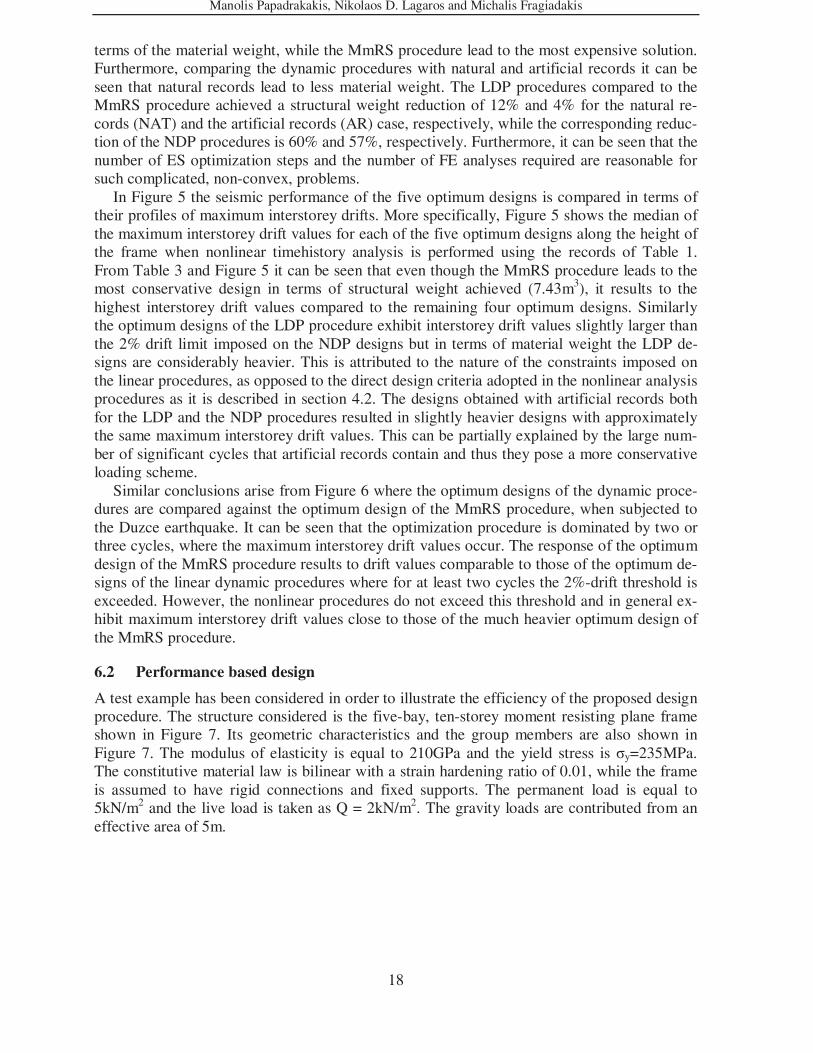
6.2 Performance based design

A test example has been considered in order to illustrate the efficiency of the proposed design procedure. The structure considered is the five-bay, ten-storey moment resisting plane frame shown in Figure 7. Its geometric characteristics and the group members are also shown in Figure 7. The modulus of elasticity is equal to 210GPa and the yield stress is σy=235MPa. The constitutive material law is bilinear with a strain hardening ratio of 0.01, while the frame is assumed to have rigid connections and fixed supports. The permanent load is equal to 5kN/m2 and the live load is taken as Q = 2kN/m2. The gravity loads are contributed from an effective area of 5m.

Manolis Papadrakakis, Nikolaos D. Lagaros and Michalis Fragiadakis

19

Figure 7 Geometry and member grouping

The problem consists of 13 design variables which represent the cross sections of the members as shown in Figure 7. The cross-sections are W-shape available from manuals of the American Institute of Steel Construction (AISC). More specifically all beams are chosen from a database of 23 W21 sections and all columns are chosen from a database of 37 W14 cross sections.

0 0.5 1 1.5 2 2.5 3 3.5 40

0.2

0.4

0.6

0.8

1

1.2

1.4

1.6

1.8

2

T (sec)

Sa

(g)

2% in 50yrs

50% in 50yrs

Figure 8 Uniform EC8 hazard spectra with 2% and 50% in 50 yrs probability of being exceeded

Seismic hazard is represented by the EC8 spectrum where two uniform hazard spectra for the 2% and the 50% earthquakes are obtained using peak ground acceleration values of 0.60g and 0.12g, respectively (Figure 8). Moreover, the importance factor γI was taken equal to 1 and the characteristic periods TA and TB of the spectrum were considered equal to 0.15 and 0.60sec (soil type B), respectively. All records are scaled to match the 5% damped EC8

Manolis Papadrakakis, Nikolaos D. Lagaros and Michalis Fragiadakis

20

elastic response spectrum at the first mode Sa(T1,5%). The slope k of the hazard curve of Eq. (6) is obtained from the expression (FEMA-350, Appendix A):

( )( ) ( )

50 /50 2 /50

50 /50 2/ 50 50 /50 2 /501 1 1 1

ln / 3.53

ln ( ) / ( ) ln ( ) / ( )

Si SiH Hk

Sa T Sa T Sa T Sa T= =

(13)

Where 50/ 50 2 /50andSi SiH H are the probabilities of exceedance for the two earthquakes and

1( )Sa T is the 5% damped spectral acceleration at the first mode of each candidate design ob-

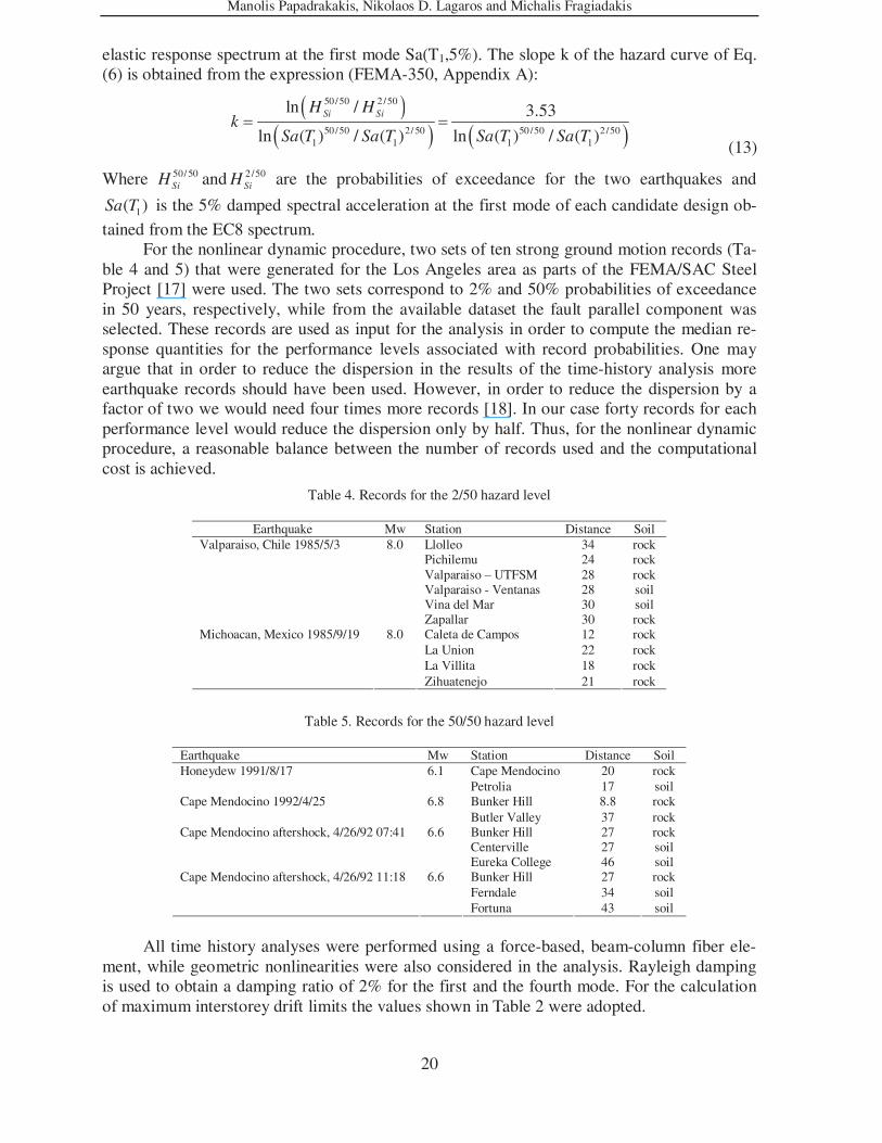
tained from the EC8 spectrum. For the nonlinear dynamic procedure, two sets of ten strong ground motion records (Ta-

ble 4 and 5) that were generated for the Los Angeles area as parts of the FEMA/SAC Steel Project [17] were used. The two sets correspond to 2% and 50% probabilities of exceedance in 50 years, respectively, while from the available dataset the fault parallel component was selected. These records are used as input for the analysis in order to compute the median re-sponse quantities for the performance levels associated with record probabilities. One may argue that in order to reduce the dispersion in the results of the time-history analysis more earthquake records should have been used. However, in order to reduce the dispersion by a factor of two we would need four times more records [18]. In our case forty records for each performance level would reduce the dispersion only by half. Thus, for the nonlinear dynamic procedure, a reasonable balance between the number of records used and the computational cost is achieved.

Table 4. Records for the 2/50 hazard level

Earthquake Mw Station Distance Soil Llolleo 34 rock Pichilemu 24 rock Valparaiso – UTFSM 28 rock Valparaiso - Ventanas 28 soil Vina del Mar 30 soil

Valparaiso, Chile 1985/5/3

8.0

Zapallar 30 rock Caleta de Campos 12 rock La Union 22 rock La Villita 18 rock

Michoacan, Mexico 1985/9/19 8.0

Zihuatenejo 21 rock

Table 5. Records for the 50/50 hazard level

Earthquake Mw Station Distance Soil Cape Mendocino 20 rock Honeydew 1991/8/17 6.1 Petrolia 17 soil Bunker Hill 8.8 rock Cape Mendocino 1992/4/25 6.8 Butler Valley 37 rock Bunker Hill 27 rock Centerville 27 soil

Cape Mendocino aftershock, 4/26/92 07:41 6.6

Eureka College 46 soil Bunker Hill 27 rock Ferndale 34 soil

Cape Mendocino aftershock, 4/26/92 11:18 6.6

Fortuna 43 soil

All time history analyses were performed using a force-based, beam-column fiber ele-

ment, while geometric nonlinearities were also considered in the analysis. Rayleigh damping is used to obtain a damping ratio of 2% for the first and the fourth mode. For the calculation of maximum interstorey drift limits the values shown in Table 2 were adopted.

Manolis Papadrakakis, Nikolaos D. Lagaros and Michalis Fragiadakis

21

Table 6. Optimal and Sub-optimal Solutions

Nonlinear Static Analysis Nonlinear Dynamic Analysis Section A B C D A B C D

1 W21x57 W21x101 W21x101 W21x101 W21x128 W21x147 W21x122 W21x132 2 W21x68 W21x83 W21x68 W21x73 W21x146 W21x83 W21x101 W21x101 3 W21x57 W21x44 W21x44 W21x44 W21x217 W21x93 W21x68 W21x62 4 W21x57 W21x68 W21x83 W21x44 W21x161 W21x50 W21x68 W21x44 5 W21x57 W21x44 W21x44 W21x44 W21x307 W21x73 W21x57 W21x44 6 W14x655 W14x257 W14x99 W14x99 W14x455 W14x257 W14x193 W14x109 7 W14x730 W14x311 W14x233 W14x99 W14x730 W14x550 W14x342 W14x193 8 W14x550 W14x455 W14x426 W14x257 W14x500 W14x455 W14x426 W14x193 9 W14x730 W14x370 W14x145 W14x109 W14x500 W14x311 W14x283 W14x120

10 W14x808 W14x342 W14x211 W14x211 W14x808 W14x550 W14x550 W14x550 11 W14x605 W14x257 W14x211 W14x176 W14x605 W14x311 W14x311 W14x311 12 W14x808 W14x426 W14x211 W14x99 W14x808 W14x455 W14x257 W14x145 13 W14x605 W14x398 W14x132 W14x99 W14x505 W14x283 W14x109 W14x109

Volume (m3) 38.49 22.44 15.28 13.06 38.85 27.31 23.22 20.07 50/50 drift 0.0194 0.0211 0.0284 0.0296 0.0138 0.0143 0.0145 0.0146 2/50 drift 0.0504 0.0596 0.0745 0.0718 0.0353 0.0371 0.0400 0.0392

0

10

20

30

40

0 50 100 150 200 250

Generation

Wei

gh

t (m

3 )

NDP

NSP

A=A (38.8 m3)

B (27.3 m3)

D (20.1 m3)

C (23.2 m3)

B (22.6 m3)

C (15.3 m3)

D (13.1 m3)

Figure 9 Generation history

Following the optimization procedure described in the previous sections the ES optimi-zation history is shown in Figure 9 for both analysis procedures where the reduction in mate-rial weight with respect to the number of ES generations is shown. For each procedure, four designs A, B, C and D are identified in Figure 3 and are also listed in Table 6. Designs A are the best designs in terms of the weight value of the initial population corresponding to ran-domly chosen designs close to the upper bounds of the design variables. Designs B and C are sub-optimal designs corresponding to the best designs achieved until the 50th and the 110th generation (25% and 50% of the total number of generations), respectively. The global optima for the two procedures are designs D. Design D in the case of the NDP procedure has been achieved after 210 generations while in the case of the NSP procedure 215 generations are required. For the optimization problem examined, the type of analysis procedure did not in-fluence considerably the required number of generations. However, due to the complexity of the problem more than 200 generations were required. It can be seen (Figure 9) that compared to the static analysis procedure the dynamic procedure produces more conservative results. Although, the variability in the results due to the analysis procedure adopted has been ac-

Manolis Papadrakakis, Nikolaos D. Lagaros and Michalis Fragiadakis

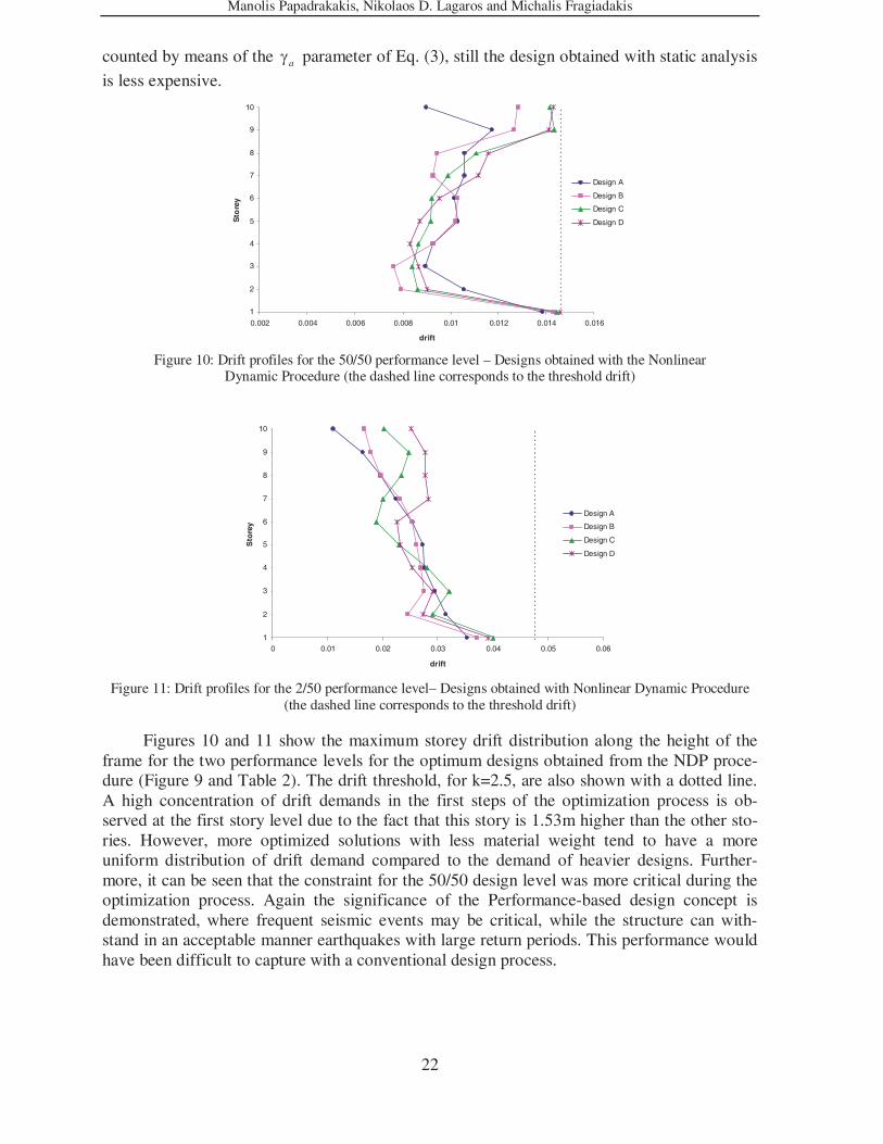
22

counted by means of the aγ parameter of Eq. (3), still the design obtained with static analysis

is less expensive.

1

2

3

4

5

6

7

8

9

10

0.002 0.004 0.006 0.008 0.01 0.012 0.014 0.016

drift

Sto

rey

Design A

Design B

Design C

Design D

Figure 10: Drift profiles for the 50/50 performance level – Designs obtained with the Nonlinear Dynamic Procedure (the dashed line corresponds to the threshold drift)

1

2

3

4

5

6

7

8

9

10

0 0.01 0.02 0.03 0.04 0.05 0.06

drift

Sto

rey

Design A

Design B

Design C

Design D

Figure 11: Drift profiles for the 2/50 performance level– Designs obtained with Nonlinear Dynamic Procedure (the dashed line corresponds to the threshold drift)

Figures 10 and 11 show the maximum storey drift distribution along the height of the frame for the two performance levels for the optimum designs obtained from the NDP proce-dure (Figure 9 and Table 2). The drift threshold, for k=2.5, are also shown with a dotted line. A high concentration of drift demands in the first steps of the optimization process is ob-served at the first story level due to the fact that this story is 1.53m higher than the other sto-ries. However, more optimized solutions with less material weight tend to have a more uniform distribution of drift demand compared to the demand of heavier designs. Further-more, it can be seen that the constraint for the 50/50 design level was more critical during the optimization process. Again the significance of the Performance-based design concept is demonstrated, where frequent seismic events may be critical, while the structure can with-stand in an acceptable manner earthquakes with large return periods. This performance would have been difficult to capture with a conventional design process.

Manolis Papadrakakis, Nikolaos D. Lagaros and Michalis Fragiadakis

23

1

2

3

4

5

6

7

8

9

10

0 0.005 0.01 0.015 0.02 0.025 0.03 0.035

drift

Sto

rey

Design A

Design B

Design C

Design D

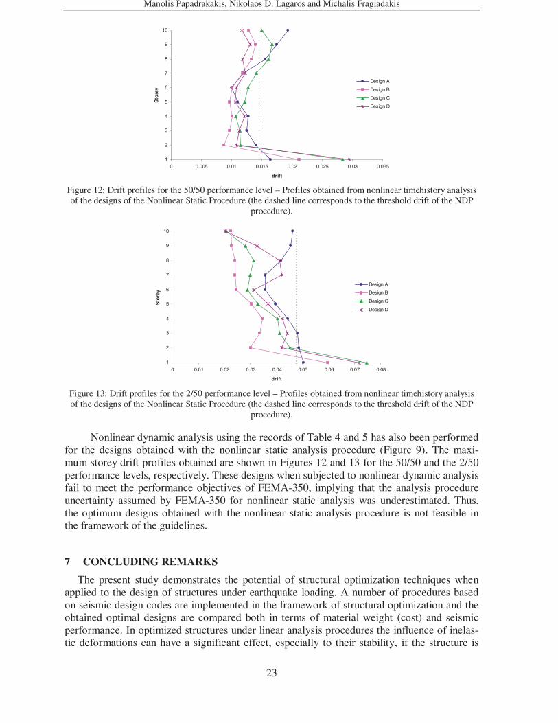
Figure 12: Drift profiles for the 50/50 performance level – Profiles obtained from nonlinear timehistory analysis of the designs of the Nonlinear Static Procedure (the dashed line corresponds to the threshold drift of the NDP

procedure).

1

2

3

4

5

6

7

8

9

10

0 0.01 0.02 0.03 0.04 0.05 0.06 0.07 0.08

drift

Sto

rey

Design A

Design B

Design C

Design D

Figure 13: Drift profiles for the 2/50 performance level – Profiles obtained from nonlinear timehistory analysis of the designs of the Nonlinear Static Procedure (the dashed line corresponds to the threshold drift of the NDP

procedure).

Nonlinear dynamic analysis using the records of Table 4 and 5 has also been performed for the designs obtained with the nonlinear static analysis procedure (Figure 9). The maxi-mum storey drift profiles obtained are shown in Figures 12 and 13 for the 50/50 and the 2/50 performance levels, respectively. These designs when subjected to nonlinear dynamic analysis fail to meet the performance objectives of FEMA-350, implying that the analysis procedure uncertainty assumed by FEMA-350 for nonlinear static analysis was underestimated. Thus, the optimum designs obtained with the nonlinear static analysis procedure is not feasible in the framework of the guidelines.

7 CONCLUDING REMARKS

The present study demonstrates the potential of structural optimization techniques when applied to the design of structures under earthquake loading. A number of procedures based on seismic design codes are implemented in the framework of structural optimization and the obtained optimal designs are compared both in terms of material weight (cost) and seismic performance. In optimized structures under linear analysis procedures the influence of inelas-tic deformations can have a significant effect, especially to their stability, if the structure is

Manolis Papadrakakis, Nikolaos D. Lagaros and Michalis Fragiadakis

24

subjected to earthquake loading since heavier linearly elastic structures do not, in general, have a better post-limit response. In order to circumvent this problem the use of alternative design approaches based on more elaborate analysis procedures is suggested. The numerical results demonstrate that more elaborate analysis procedures take explicitly into account the characteristics of the seismic response and thus lead to designs with better seismic perform-ance. Furthermore, by avoiding conservative designs checks and assumptions made by simpli-fying procedures, structural designs with less material weight can be obtained.

The main conclusions of the presented evaluation of optimum seismic design procedures are the following: (i) improved control on the structural response and weight is achieved when non-linear analysis is performed, compared to optimum designs obtained when linear analysis procedures based on EC8 requirements were adopted; (ii) a reasonable number ES optimiza-tion steps, and thus designs with affordable computational cost, with substantially less mate-rial cost can be obtained; (iii) the use of artificial instead of natural ground motion records leads to slightly heavier structures since they constitute a more ‘demanding’ loading scheme. It was also demonstrated that the Evolution Strategies algorithm can be considered not only a robust but also an efficient tool for design optimization of real world space frames under earthquake loading. Furthermore a framework for the performance-based optimal design of steel structures has also been proposed in this study. Two different analytical procedures, nonlinear static analysis and nonlinear dynamic analysis were implemented in order to deter-mine the level of damage for two performance levels. In order to account for a number of un-certainties which are critical for the determination of the structural response for each performance level, the FEMA-350 methodology has been adopted. It is shown that structural code design checks can be implemented in a straightforward manner when nonlinear analysis procedures are adopted and optimum designs that meet the specified performance objectives with the desired confidence can be obtained.

REFERENCES

[1] Han SW, Wen YK. Method for reliability-based seismic design: Equivalent nonlinear systems, II: Calibration of code parameters. ASCE Journal of Structural Engineering 1997; 123(3): 256-270.

[2] Bazzuro P, Cornell CA, Shome N, Carballo JE. Three proposals for characterizing MDOF nonlinear response. ASCE Journal of Structural Engineering 1998; 124(11): 1281-1289.

[3] Foley CM. Optimized performance-based design for buildings. In Burns S.A. (Ed.) Re-cent Advances in Optimal Structural Design, ASCE Publications, 2002: 169-240.

[4] Polak E, Pister KS, Ray D. Optimal design of framed structures subjected to earth-quakes. Engineering Optimization 1976; 2: 65-71.

[5] Bhatti MA, Pister KS. A dual criteria approach for optimal design of earthquake resis-tant structural systems. Earthquake Engineering and Structural Dynamics 1981; 9: 557-572.

[6] Balling RJ, Ciampi V, Pister KS, Polak E. Optimal design of seismic-resistant planar steel frames. Earthquake Engineering Research Center, University of California, Berke-ley. Report No. UCB/EERC-81/20, 1981.

Manolis Papadrakakis, Nikolaos D. Lagaros and Michalis Fragiadakis

25

[7] Pezeshk S. Design of framed structures: an integrated non-linear analysis and optimal minimum weight design. International Journal for Numerical Methods in Engineering 1998; 41: 459-471.

[8] Charney FA.. Needs in the Development of a comprehensive performance based opti-mization process. In Elgaaly M. (Ed.) ASCE Structures 2000 Conference Proceedings. May 8–10; 2000, Philadelphia, Pennsylvania, USA; Paper No. 28.

[9] Ganzerli S, Pantelides CP, Reaveley LD. Performance-based design using structural op-timization. Earthquake Engineering and Structural Dynamics 2000; 29: 1677-1690.

[10] Esteva L, Dıaz-Lopez O, Garcıa-Perez J, Sierra G, Ismael E. Life-cycle optimization in the establishment of performance-acceptance parameters for seismic design. Structural Safety 2002; 24: 187–204.

[11] Gong Y. Performance-based design of steel building frameworks under seismic loading. PhD Thesis, Dep. of Civil Eng. University of Waterloo, Canada, 2003.

[12] Chan C-M, Zou X-K. Elastic and inelastic drift performance optimization for reinforced concrete buildings under earthquake loads, Earthquake Engineering and Structural Dy-namics 2004; 33: 929–950.

[13] Kocer FY, Arora JS. Optimal design of H-frame transmission poles for earthquake load-ing. ASCE Journal of Structural Engineering 1999; 125(11): 1299-1308.

[14] Kocer FY, Arora JS. Optimal design of latticed towers subjected to earthquake loading, ASCE Journal of Structural Engineering 2002; 128(2):197-204.

[15] Beck JL, Chan E, Irfanoglu A, Papadimitriou C. Multi-criteria optimal structural design under uncertainty. Earthquake Engineering and Structural Dynamics 1999; 28: 741-761.

[16] Cheng FY, Li D, Ger J. Multiobjective optimization of seismic structures. In Elgaaly M. (Ed.) ASCE Structures 2000 Conference Proceedings. May 8–10; 2000, Philadelphia, Pennsylvania, USA; Paper No. 24.

[17] Liu M, Burns SA, Wen YK. Optimal seismic design of steel frame buildings based on life cycle cost considerations. Earthquake Engineering and Structural Dynamics 2003; 32: 1313-1332.

[18] Liu M, Wen YK, Burns SA. Life cycle cost oriented seismic design optimization of steel moment frame structures with risk-taking preference. Engineering Structures 2004; 26: 1407-1421.

[19] Liu M, Burns SA, Wen YK. Multiobjective optimization for performance-based seismic design of steel moment frame structures. Earthquake Engineering and Structural Dy-namics 2005; 34: 289-306.

[20] FEMA 356: Prestandard and commentary for the seismic rehabilitation of buildings. Federal Emergency Management Agency, Washington DC, SAC Joint Venture, 2000.

[21] Eurocode 8. Design provisions for earthquake resistant structures. CEN-ENV, 1994.

[22] Antoniou S, Pinho R. Development and verification of a displacement-based adaptive pushover procedure, Journal of Earthquake Engineering, 2004; 8: 643:661.

[23] Chintanapakdee C, Chopra AK. Evaluation of modal pushover analysis using generic frames, Earthquake Engineering and Structural Dynamics, 2003, 32: 417-442.

Manolis Papadrakakis, Nikolaos D. Lagaros and Michalis Fragiadakis

26

[24] Eurocode 3. Design of steel structures. Part1.1: General rules for buildings. CEN- ENV, 1993.

[25] Zhu TJ, Heidebrecht AC, Tso WK. Effect of peak ground acceleration to velocity ratio on the ductility demand of inelastic systems. Earthquake Engineering and Structural Dynamics, 1988; 16: 63-79.

[26] Shome N, Cornell CA, Bazzuro P, Carballo JE. Earthquakes, records, and nonlinear re-sponses. Earthquake Spectra 1998; 14: 469-500.

[27] Gasparini DA, Vanmarke EH. Simulated earthquake motions compatible with pre-scribed response spectra. Dep. of Civil Eng. MIT, Publication No. R76-4, 1976.

[28] Argyris J, Tenek L, Mattssonn A. BEC: A 2-node fast converging shear-deformable iso-tropic and composite beam element based on 6 rigid-body and 6 straining modes. Com-puter Methods in Applied Mechanics in Engineering 1998; 152: 281-336.

[29] Papadrakakis M, Tsompanakis Y, Hinton E, Sienz J. Advanced solution methods in to-pology optimization and shape sensitivity analysis. Journal of Engineering Computa-tions 1996; 13(5): 57-90.

[30] Papadrakakis M, Tsompanakis Y, Lagaros ND. Structural shape optimization using Evolution Strategies. Engineering Optimization 1999; 31: 515-540.

[31] Papadrakakis M, Lagaros ND, Thierauf G, Cai J. Advanced solution methods in struc-tural optimization based on Evolution Strategies. Engineering Computations Journal 1998; 15: 12-34.