Sequential Parameter Optimization Appliedto Self-Adaptation for Binary-CodedEvolutionary Algorithms

Mike Preuss and Thomas Bartz-Beielstein

Dortmund University, D-44221 Dortmund, Germany.mike.preuss@cs.uni-dortmund.de, thomas.bartz-beielstein@udo.edu

Summary. Adjusting algorithm parameters to a given problem is of crucial impor-tance for performance comparisons as well as for reliable (first) results on previouslyunknown problems, or with new algorithms. This also holds for parameters con-trolling adaptability features, as long as the optimization algorithm is not able tocompletely self-adapt itself to the posed problem and thereby get rid of all para-meters. We present the recently developed sequential parameter optimization (SPO)technique that reliably finds good parameter sets for stochastically disturbed algo-rithm output. SPO combines classical regression techniques and modern statisticalapproaches for deterministic algorithms as Design and Analysis of Computer Exper-iments (DACE). Moreover, it is embedded in a twelve-step procedure that targetsat doing optimization experiments in a statistically sound manner, focusing on an-swering scientific questions.

We apply SPO to a question that did not receive much attention yet: Is self-adaptation as known from real-coded evolution strategies useful when applied tobinary-coded problems? Here, SPO enables obtaining parameters resulting in goodperformance of self-adaptive mutation operators. It thereby allows for reliable com-parison of modified and traditional evolutionary algorithms, finally allowing for wellfounded conclusions concerning the usefulness of either technique.

1 Introduction

The evolutionary computation (EC) field currently seems to experience a state offlux, at least as far as experimental research methods are concerned. A purely theo-retical approach is not reasonable for many optimization problems. In fact, there isa huge gap between theory and experiment in evolutionary computation. However,empiricism in EC cannot compensate this shortcoming due to a lack of standards.A broad spectrum of presentation techniques makes new results almost incompara-ble. At present, it is intensely discussed which experimental research methodologiesshould be used to improve the acceptance and quality of evolutionary algorithms(EA).

Several authors from related fields ([32], [57], and [39]) and from within EC ([81],[23]) have criticized usual experimental practice. Besides other topics, they ask for

M. Preuss and T. Bartz-Beielstein: Sequential Parameter Optimization Applied to Self-

Adaptation for Binary-Coded Evolutionary Algorithms, Studies in Computational Intelligence

(SCI) 54, 91–119 (2007)

www.springerlink.com © Springer-Verlag Berlin Heidelberg 2007

92 Mike Preuss and Thomas Bartz-Beielstein

increased thoughtfulness when selecting benchmark problems, a better structuredprocess of experimentation, including presentation of results, and proper use of sta-tistical techniques.

In the light of the no free lunch theorem (NFL, [82]), research aims are graduallychanging from demonstration of superiority of new algorithms towards experimentalanalysis, addressing questions as: What makes an algorithm work well on a certainproblem class? In spite of this development, the so-called horse race papers1 stillseem to prevail. [23] report about the situation in experimental EC and name thereasons for their discontentment with current practice. Put into positive formulation,their main demands are:

• assembly of concrete research questions and concrete answers to these, no claimsthat are not backed up by tests

• selection of test problems and instances motivated by these questions• utilization of adequate performance measures for answering the questions, and• reproducibility, which requires all necessary details and/or source code to repeat

experimentsThis line is carried further in [22]. Partly in response to these demands, [7] pro-poses SPO as a structured experimentation procedure based on modern statistictechniques (§4). In its heart, SPO contains a parameter tuning method that enablesadapting parameters to the treated test problems.

Undoubtedly, comparing badly parametrized algorithms is rather useless. How-ever, a good parameter set allows for near-optimal performance of an algorithm.As this statement suggests, parameter tuning is of course an optimization problemon its own. Following from that, some interesting questions arise when algorithmswith parameter control operators are concerned, because their own adaptability is inturn guarded by control parameters, which can be tuned. The broadest of these ques-tions may be where to put effort into when striving for best performance—tune thesimple algorithm, or tune the adaptability of more complex algorithms—eventuallyresulting in recommendations when to apply adaptive operators.

1.1 Parameter Control or Parameter Tuning?

Parameter Control refers to parameter adaptation during the run of an optimizationalgorithm, whereas parameter tuning improves their setting before the run is started.These two different mechanisms are the roots of the two subtrees of parameter settingmethods in the global taxonomy given by [21]. One may get the impression that theyare contradictory and researchers should aim at using parameter control as much aspossible. In our view, the picture is somewhat more complex, and the two are rathercomplementary.

In a production environment, an EA and any alternative stochastic optimizationalgorithm would be run several times, not once, possibly solving the next or tryingthe same problem again. This obliterates the separating time factor of above. Whatis more, the EA as well as the problem representation will most likely undergostructural changes during these iterations (new operators, criteria, etc.). These willentail changes in the “optimal” parameters, too.

1 [39] uses this term for papers that aim at showing predominance of one algo-rithm over (all) others by reporting performance comparisons on (standard) testproblems.

SPO Applied to Self-Adaptation for Binary-Coded EAs 93

Furthermore, parameter control methods do not necessarily decrease the numberof parameters. For example, the 1/5th adaptation rule by [63] provides at least threequantities where there has been one—mutation step size—before, namely the timewindow length used to measure success, the required success rate (1/5), and the rateof change applied. Even if their number remains constant, is it justified to expectthat parameter tuning has become simpler now? We certainly hope so, but needmore evidence to decide.

In principle, every EA parameter may be (self-)adapted. However, concurrentadaptation of many does not seem particularly successful and is probably limitedto two or three at a time. We thus cannot simply displace parameter tuning withparameter control. On the other hand, manual tuning is surely not the answer, aswell, and grid based tuning seems intractable for higher order design spaces. At thispoint, we have three possibilities, either to

• fall back on default values,• abandon tuning alltogether and take random parameters, or• to apply a tuning method that is more robust than doing it manually, but also

more efficient than grid search.We argue that SPO is such a method and thus of particular importance for

experimental studies on non-trivial EAs, as such utilizing self-adaptation. As theexperimental analysis in EC currently is a hot topic, other parameter tuning ap-proaches are developed, too, e.g. [61]. But whatever method is used, there is hardlya way around parameter tuning, at least for scientific investigations. SPO will bediscussed further in §4.

1.2 Self-adaptation for Binary Representations

When comparing recent literature, it is astounding that for real-coded EAs as e.g.evolution strategies (ES), self-adaptation is an almost ubiquitously applied feature,at least as far as mutation operators are concerned. In binary-coded EA however,it did not become a standard method. Optimization practitioners working withbinary representations seem largely unconvinced that it may be of any use. Whatmay be the reason for this huge difference? One could first think of traditionalreasons. Of the three standard evolutionary methods for numerical optimization,genetic algorithms (GA), evolutionary programming (EP) and evolution strategies,the last one first adopted self-adaptation in various forms to improve mutationoperators ([64, 71, 72]), followed by EP in [25]. These two mainly work with real-valued representations. Nevertheless, since then so much time has passed that it ishard to imagine that others would not employ a technique that clearly provides anadvantage. Considering this, tradition appears not as a substantial reason for thedivergent developments.

In fact, meanwhile, several authors have tried to transfer self-adaptation to EAsfor binary encodings: [4, 3, 70, 74, 75, 77, 29]. If we accept the view of an evolutionaryepistemology underlying the development of our scientific domain, so that mostlysuccessful changes are inherited to the next stages, these studies have apparentlynot been very convincing. Either they were ignored by the rest of the field, or theyfailed to provide reason good enough for a change. Let us assume the latter case.In consequence, most EAs for binary representations published nowadays still dowithout self-adaptation.

94 Mike Preuss and Thomas Bartz-Beielstein

Evolutionary algorithms employing different forms of self-adaptation are usuallyapplied to continuous, or, more rarely, ordinal discrete or mixed search spaces. Sothe distinction may result from differences in representation. When dealing withreal-valued numbers, it is quite easy to come by a good intuition why adaptingmutation strengths (also called mutation step sizes) during optimization can speedup search. Features of a fitness landscape changing slowly compared to the fitnessvalues themselves can be learned, like gradients or covariances ([31, 30]). In a binaryspace, this intuition is lacking. Definition of gradients is meaningless if a variablecan only take two values. Consequently, research is trying different ways here, e.g.linkage learning or distribution estimation as in [59]. As much as the experiences fromcontinuous search spaces cannot be simply transferred, neither can the methods. Self-adaptation of mutation rates, as straightforward continuation of existing techniquesfor real-valued variables, if working at all for binary representations, can be expectedto work differently.

2 Aims and Methods

Our aims are twofold: To demonstrate usefulness of the SPO approach for experimen-tal analysis, and to perform an experimental analysis of self-adaptation mechanisms.

Methodologically, we want to convey that SPO is a suitable tool for finding goodparameter sets (designs) within a fixed, low budget of algorithm runs. It seems safeto assume that a parameter set exists in the parameter design space that is betterthan the best of a small (≈100) sample. We therefore require that the best config-urations detected by SPO are significantly better than the best of a first sample.Furthermore, we want to suggest a flexible yet structured methodology for perform-ing and documenting experimentation by employing a parameter tuning technique.

Concerning the experimental analysis of self-adaptation mechanisms on binaryrepresented problems, our aim is to collect evidence for or against the followingconjectures:

• Well parametrized self-adaptation significantly speeds up optimization whencompared to well tuned constant mutation rates for many problems.

• Detecting good parameter sets for self-adaptive EAs is usually not significantlyharder than doing so for non self-adaptive EAs.

• Problem knowledge, e.g., shared properties or structural similarities of problemclasses, gives useful hints for selecting a self-adaptation mechanism.

Before these conjectures are detailed, we give an overview of existing parametertuning methods.

3 Parameter Optimization Approaches

Modern search heuristics have proved to be very useful for solving complex real–world optimization problems that cannot be tackled through classical optimizationtechniques [73]. Many of these search heuristics involve a set of exogenous parame-ters, i.e., values are specified before the run is performed, that affect their conver-gence properties. The population size in EA is a typical example for an exogenousstrategy parameter. The determination of an adequate population size is crucial for

SPO Applied to Self-Adaptation for Binary-Coded EAs 95

many optimization problems. Increasing the population size from 10 to 50 whilekeeping the number of function evaluations constant might improve the algorithm’sperformance—whereas a further increase might result in a performance decrease, ifthe number of function evaluations remains constant.

SPO is based on statistical design of experiments (DOE) which has its ori-gins in agriculture and industry. However, DOE has to be adapted to the specialrequirements of computer programs. For example, computer program are per se de-terministic, thus a different concepts of randomness has to be considered. Law &Kelton [46] and Kleijnen [43, 44] demonstrated how to apply DOE in simulation.Simulation is related to optimization (simulation models equipped with an objec-tive function define a related optimization problem), therefore we can benefit fromsimulation studies.

DOE related parameter studies were performed to analyze EA: Schaffer et al. [67]proposed a complete factorial design experiment, Feldt & Nordin [24] use statisti-cal techniques for designing and analyzing experiments to evaluate the individualand combined effects of genetic programming parameters. Myers & Hancock [58]presented an empirical modeling of genetic algorithms. Francois & Lavergne [26]demonstrate the applicability of generalized linear models to design evolutionaryalgorithms. These approaches require up to 100,000 program runs, whereas SPO isapplicable even if a small amount of function evaluations are available only.

Because the search for useful parameter settings of algorithms itself is an opti-mization problem, meta-algorithms have been proposed. Back [2] and Kursawe [45]presented meta-algorithms for evolutionary algorithms. But these approaches do notsolve the original problem completely, because they require the determination of ad-ditional parameter setting of the meta-algorithm. Furthermore, we argue that theexperimenter’s skill plays an important role in this analysis. It cannot be replacedby automatic “meta” rules.

SPO can also be run on auto-pilot without any user intervention. This conve-nience cannot be obtained for free: The user gains limited insight into the workingmechanisms of the tuned algorithm and, which is even more severe, the validity andthus the predictive power of the regression model might be quite poor.

The reader should note that our approach is related to the discipline of experi-mental algorithmics, which offers methodologies for the design, implementation, andperformance analysis of computer programs for solving algorithmic problems [18,56]. Further valuable approaches have been proposed by McGeoch [50], Barr &Hickman [5], and Hooker [32].

Design and analysis of computer experiments (DACE) as introduced in Sackset al. [65] models the deterministic output of a computer experiment as the realiza-tion of a stochastic process. The DACE approach focuses entirely on the correlationstructure of the errors and makes simplistic assumptions about the regressors. Itdescribes “how the function behaves,” whereas regression as used in classical DOE

describes “what the function is” [40, p. 14]. DACE requires other experimental de-signs than classical DOE, e.g., Latin hypercube designs (LHD) [51].

We claim that it is beneficial to combine some of these well-established ideasfrom DOE, DACE, and further statistical techniques to improve the acceptanceand quality of evolutionary algorithms.

96 Mike Preuss and Thomas Bartz-Beielstein

4 Sequential Parameter Optimization Methodology

How can optimization practitioners determine if concepts developed in theory workin practice? Hence, experiments are necessary. Experiment has a long tradition inscience. To analyze experimental data, statistical methods can be applied. It is nota trivial task to answer the final question “Is algorithm A better than algorithm B?”Results that are statistically significant are not automatically scientifically mean-ingful.

Example 4.1 (Floor and ceiling effects). The statistical meaningful result “allalgorithms perform equally” can be scientifically meaningless, because the probleminstances are too hard for any algorithm. A similar effect occurs if the probleminstances are too easy. The resulting effects are known as floor or ceiling effects,respectively. �

SPO is more than a simple combination of existing statistical approaches. It is basedon the new experimentalism, a development in the modern philosophy of science,which considers that an experiment can have a life of its own. SPO provides astatistical methodology to learn from experiments, where the experimenter shoulddistinguish between statistical significance and scientific meaning.

An optimization run is considered as an experiment. An optimal parameter set-ting, or statistically speaking, an optimal algorithm design, depends on the problemat hand as well as on the restrictions posed by the environment (i.e., time and hard-ware constraints). Algorithm designs are usually either determined empirically orset equal to widely used default values. SPO is a methodology for the experimentalanalysis of optimization algorithms to determine improved algorithm designs andto learn, how the algorithm works. The proposed technique employs computationalstatistic methods to investigate the interactions among optimization problems, algo-rithms, and environments.

An optimization practitioner is interested in robust solutions, i.e., solutions inde-pendent from the random seeds that are used to generate the random numbers duringthe optimization run. The proposed statistical methodology provides guidelines todesign robust algorithms under restrictions, such as a limited number of functionevaluations and processing units. These restrictions can be modeled by consideringthe performance of the algorithm in terms of the (expected) best function value fora limited number of function evaluations.

To justify the usefulness of our approach, we analyze the properties of severalalgorithms from the viewpoint of a researcher who wants to develop and understandself-adaptation mechanisms for evolutionary algorithms. SPO provides numericaland graphical tools to test if the statistical results are really relevant or have beencaused by the experimental setup only. It is based on a framework that permits a de-linearization of the complex steps from raw data to scientific hypotheses. Substantivescientific questions are broken down into several local hypotheses, that can be testedexperimentally. The optimization process can be regarded as a process that enableslearning. SPO consists of the twelve steps that are reported in Table 1. These stepsand the necessary statistical techniques will be presented in the following. SPO hasbeen applied on search heuristics in the following domains:

1. machine engineering: design of mold temperature control [53, 80, 52]2. aerospace industry: airfoil design optimization [11]

SPO Applied to Self-Adaptation for Binary-Coded EAs 97

3. simulation and optimization: elevator group control [13, 49]4. technical thermodynamics: nonsharp separation [10]5. economy: agri-environmental policy-switchings [17]

Other fields of application are in fundamental research:

1. algorithm engineering: graph drawing [79]2. statistics: selection under uncertainty (optimal computational budget alloca-

tion) for PSO [8]3. evolution strategies: threshold selection and step-size adaptation [6]4. other evolutionary algorithms: genetic chromodynamics [76]5. computational intelligence: algorithmic chemistry [10]6. particle swarm optimization: analysis and application [9]7. numerics: comparison and analysis of classical and modern optimization algo-

rithms [12]

Further projects, e.g., vehicle routing and door-assignment problems and the appli-cation of methods from computational intelligence to problems from bioinformaticsare subject of current research. An SPO-toolbox is freely available under the follow-ing link: http://www.springer.com/3-540-32026-1.

4.1 Tuning

In order to find an optimal algorithm design, or to tune the algorithm, it is necessaryto define a performance measure. Effectivity (robustness) and efficiency can guide

Table 1. Sequential parameter optimization (SPO). This approach combines meth-ods from computational statistics and exploratory data analysis to improve (tune)the performance of direct search algorithms.

Step Action

(S-1) Preexperimental planning(S-2) Scientific claim(S-3) Statistical hypothesis(S-4) Specification of the

(a) optimization problem(b) constraints(c) initialization method(d) termination method(e) algorithm (important factors)(f) initial experimental design(g) performance measure

(S-5) Experimentation(S-6) Statistical modeling of data and prediction(S-7) Evaluation and visualization(S-8) Optimization(S-9) Termination: If the obtained solution is good enough, or the maximum num-

ber of iterations has been reached, go to step (S-11)(S-10) Design update and go to step (S-5)(S-11) Rejection/acceptance of the statistical hypothesis(S-12) Objective interpretation of the results from step (S-11)

98 Mike Preuss and Thomas Bartz-Beielstein

the choice of an adequate performance measure. Note that optimization practitionersdo not always choose the absolute best algorithm. Sometimes a robust algorithm oran algorithm that provides insight into the structure of the optimization problemis preferred. From the viewpoint of an experimenter, design variables (factors) arethe parameters that can be changed during an experiment. Generally, there are twodifferent types of factors that influence the behavior of an optimization algorithm:

• problem specific factors, e.g., the objective function• algorithm specific factors, i.e., the population size or other exogenous parameters

We will consider experimental designs that comprise problem specific factors andexogenous algorithm specific factors. Algorithm specific factors will be consideredfirst. Endogenous can be distinguished from exogenous parameters [16]. The formerare kept constant during the optimization run, whereas the latter, e.g., standarddeviations, are modified by the algorithms during the run. Consider DA, the set ofall parameterizations for one algorithm. An algorithm design XA is a set of vectors,each representing one specific setting of the design variables of an algorithm. A designcan be specified by defining ranges of values for the design variables. A design pointxa ∈ DA presents exactly one parameterization of an algorithm. Note that a designcan contain none, one, several or even infinitely many design points. The optimalalgorithm design is denoted as X∗

A. The term “optimal design” can refer to the bestdesign point x∗

a as well as the most informative design points [60, 66].Let DP denote the set of all problem instances for one optimization problem.

Problem designs XP provide information related to the optimization problem, suchas the available resources (number of function evaluations) or the problem’s dimen-sion.

An experimental design XE ∈ D consists of a problem design XP and an al-gorithm design XA. The run of a stochastic search algorithm can be treated as anexperiment with a stochastic output Y (xa, xp), with xa ∈ DA and xp ∈ DP . If therandom seed is specified, the output would be deterministic. This case will not beconsidered further, because it is not a common practice to specify the seed that isused in an optimization run. Our goals of the experimental approach can be statedas follows:

(G-1) Efficiency. To find a design point x∗a ∈ DA that improves the performance of

an optimization algorithm for one specific problem design point xp ∈ DP .(G-2) Robustness. To find a design point x∗

a ∈ DA that improves the performanceof an optimization algorithm for several problem design points xp ∈ DP .

Performance can be measured in many ways, e.g., as the best or the average functionvalue for n runs. Statistical techniques to attain these goals will be presented next.

4.2 Stochastic Process Models as Extensions of ClassicalRegression Models

The classical DOE approach consists of three steps: Screening, modeling, and opti-mization. Each step requires different experimental designs. Linear regression mod-els are central elements of the classical design of experiments approach [19, 55]. Wepropose an approach that extends the classical regression techniques, because theassumption of a linear model for the analysis of computer programs and the implicit

SPO Applied to Self-Adaptation for Binary-Coded EAs 99

model assumption that observation errors are independent of one another are highlyspeculative [7]. To keep the number of experiments low, a sequential procedure hasbeen developed. Our approach relies on a stochastic process model, that will bepresented next.

We consider each algorithm design with associated output as a realization of astochastic process. Kriging is an interpolation method to predict unknown valuesof a stochastic process and can be applied to interpolate observations from com-putationally expensive simulations. Our presentation follows concepts introduced inSacks et al. [65], Jones et al. [40], and Lophaven et al. [48].

Consider a set of m design points x = (x(1), . . . , x(m))T with x(i) ∈ Rd. In the

design and analysis of computer experiments (DACE) stochastic process model, adeterministic function is evaluated at the m design points x. The vector of the mresponses is denoted as y = (y(1), . . . , y(m))T with y(i) ∈ R. The process modelproposed in Sacks et al. [65] expresses the deterministic response y(x(i)) for a d-dimensional input x(i) as a realization of a regression model F and a stochasticprocess Z,

Y (x) = F(β, x) + Z(x). (1)

DACE Regression Models

We use q functions fj : Rd → R to define the regression model

F(β, x) =

q∑

j=1

βjfj(x) = f(x)T β. (2)

Regression models with polynomials of orders 0, 1, and 2 have been used in ourexperiments. Regression models with a constant term only, i.e., f1 = 1, have beenapplied successfully to model the data and to predict new data points in the sequen-tial approach.

DACE Correlation Models

The random process Z(·) (Equation 1) is assumed to have mean zero and covarianceV (w, x) = σ2R(θ, w, x) with process variance σ2 and correlation model R(θ, w, x).Consider an algorithm with d factors (parameters). Correlations of the form

R(θ, w, x) =

d∏

j=1

Rj(θ, wj − xj)

will be used in our experiments. The correlation function should be chosen withrespect to the underlying process [34]. Lophaven et al. [47] discuss seven differentmodels. The Gaussian correlation function is a well-known example. It is defined as

GAUSS : Rj(θ, hj) = exp(−θjh2j ), (3)

with hj = wj − xj , and for θj > 0. The regression matrix R is the matrix withelements

Rij = R(xi, xj) (4)

100 Mike Preuss and Thomas Bartz-Beielstein

that represent the correlations between Z(xi) and Z(xj). The vector with correla-tions between Z(xi) and a new design point Z(x) is

r(x) = (R(x1, x), . . . , R(xm, x)) . (5)

Large θj ’s indicate that variable j is active: function values at points in the vicinityof a point are correlated with Y at that point, whereas small θj ’s indicate thatalso distant data points influence the prediction at that point. The empirical bestunbiased linear predictor (EBLUP) can be shown to be

y(x) = fT (x)β + rT (x)R−1(y − F β), (6)

whereβ =

(F T R−1F

)−1F T R−1y (7)

is the generalized least-squares estimate of β in Equation 1, f(x) are the q regressionfunctions in Equation 2, and F represents the values of the regression functions inthe m design points.

Maximum likelihood estimation methods to estimate the parameters θj of thecorrelation functions from Equation 3 are discussed in Lophaven et al. [47]. DACEmethods provide an estimation of the prediction error on an untried point x, themean squared error (MSE) of the predictor

MSE(x) = E (y(x) − y(x)) . (8)

The stochastic process model, which was introduced as an extension of the classicalregression model will be used in our experiments. Next, we have to decide how togenerate design points, i.e., which parameter settings should be used to test thealgorithm’s performance.

Space Filling Designs and Expected Improvement

Often, designs that use sequential sampling are more efficient than designs with fixedsample sizes. Therefore, we specify an initial design X

(0)A ∈ D(0)

A first. Latin hyper-cube sampling (LHS) was used to generate the initial algorithm designs. Consider nnumber of levels being examined and d design variables. A Latin hypercube is a ma-trix of n rows and d columns. The d columns contain the levels 1, 2, . . . , n, randomlypermuted, and the d columns are matched at random to form the Latin hypercube.The resulting Latin hypercube designs are space-filling designs. McKay et al. [51] in-troduced LHDs for computer experiments, Santner et al. [66] give a comprehensiveoverview.

Information obtained in the first runs can be used for the determination of thesecond design X

(1)A in order to choose new design points sequentially and thus more

efficiently.Sequential sampling approaches have been proposed for DACE. For example,

in Sacks et al. [65] sequential sampling approaches were classified to the existingmeta-model. We will present a sequential approach that is based on the expectedimprovement. In Santner et al. [66, p. 178] a heuristic algorithm for unconstrainedglobal minimization problems is presented. Consider one problem design point xp.

Let y(t)min denote the smallest known minimum value after t runs of the algorithm,

SPO Applied to Self-Adaptation for Binary-Coded EAs 101

SequentialParameterOptimization(DA,DP )1 Select p ∈ DP and set t = 0 /* Select problem instance */

2 X(t)A = {x1, x2, . . . , xk} /* Sample k initial points, e.g., LHS */

3 repeat4 yij = Yj(xi, p)∀xi ∈ X

(t)A and j = 1, . . . , r(t) /* Fitness evaluation */

5 Y(t)i =

∑r(t)

j=1y(t)ij /r(t) /* Sample statistic for the ith design point */

6 xb with b = arg mini(yi) /* Determine best point */7 Y (x) = F(β, x) + Z(x) /* DACE model from Eq. 1 */8 XS = {xk+1, . . . , xk+s} /* Generate s sample points, s � k */9 y(xi), i = 1, . . . , k + s /* Predict fitness from DACE model */

10 I(xi) for i = 1, . . . , s + k /* Expected improvement (Eq. 9) */

11 X(t+1)A = X

(t)A ∪ {xk+i}m

i=1 /∈ X(t)A /* Add m promising points */

12 if x(t)b = x

(t+1)b

13 then r(t+1) = 2r(t) /* Increase number of repeats */14 t = t + 1 /* Increment iteration counter */15 until BudgetExausted?()

Fig. 1. Sequential parameter optimization

y(x) be the algorithm’s response, i.e., the realization of Y (x) in Equation (1), andlet xa represent a specific design point from the algorithm design XA. Then theimprovement is defined as

I(xa) =

{y(t)min − y(xa), y

(t)min − y(xa) > 0

0, otherwise(9)

for xa ∈ DA. As Y (·) is a random variable, its exact value is unknown. The goal isto optimize its expectation, the so-called expected improvement . New design points,which are added sequentially to the existing design, are attractive “if either thereis a high probability that their predicted output is below [minimization] the cur-rent observed minimum and/or there is a large uncertainty in the predicted out-put.” This leads to the expected improvement heuristic [7]. Based on theorems fromSchonlau [68, p. 22] we implemented a program to estimate and plot the main fac-tor effects. Furthermore, three dimensional visualizations produced with the DACE

toolbox [48] can be used to illustrate the interaction between two design variablesand the associated mean squared error of the predictor.

Figure 1 describes the SPO in a formal manner. The selection of a suitableproblem instance is done in the pre-experimental planning phase to avoid floor andceiling effects (l.2). Latin hypercube sampling can be used to determine an initial setof design points (l.3). After the algorithm has been run with these k initial parametersettings (l.5), the DACE process model is used to discover promising design points(l.10). Note that other sample statistics than the mean, e.g., the median, can beused in l.6. The m points with the highest expected improvement are added tothe set of design points, where m should be small compared to s. The update rulefor the number of reevaluations r(t) (l.13–15) guarantees that the new best design

point x(t+1)b has been evaluated at least as many times as the previous best design

point x(t)b . Obviously, this is a very simple update rule and more elaborate rules

102 Mike Preuss and Thomas Bartz-Beielstein

are possible. Other termination criteria exist besides the budget based termination(l.17).

4.3 Experimental Reports

Surprisingly, despite around 40 years of empirical tradition, in EC a standardizedscheme for reporting experimental results never developed. The natural sciences, e.g.physics, possess such schemes as de-facto standards. We argue that for both groups,readers and writers, an improved report structure is beneficial: As with the com-mon overall paper structure (introduction, conclusions, etc.), a standard providesguidelines for readers, what to expect, and where. Writers are steadily reminded todescribe the important details needed to understand and possibly replicate their ex-periments. For the structured documentation of experiments, we propose organizingtheir presentation into 7 parts, as follows.ER-1: Focus/Title

Briefly names the matter dealt with, the (possibly very general) objective,preferably in one sentence.

ER-2: Pre-experimental planningReports the first—possibly explorative—program runs, leading to task and setup(steps ER-3 and ER-4) . Decisions on used benchmark problems or performancemeasures may often be influenced by the outcome of preliminary runs. Thismay also include negative results, e.g. modifications to an algorithm that didnot work, or a test problem that turned out to be too hard, if they provide newinsight.

ER-3: TaskConcretizes the question in focus and states scientific and derived statistical hy-potheses to test. Note that one scientific hypothesis may require several, some-times hundreds of statistical hypotheses. In case of a purely explorative study,as with the first test of a new algorithm, statistical tests may be not applicable.Still, the task should be formulated as precise as possible.

ER-4: SetupSpecifies problem design and algorithm design, containing fixed and variableparameters and criteria of tackled problem, investigated algorithm and chosenperformance measuring. The information in this part should be sufficient toreplicate an experiment.

ER-5: Experimentation/VisualizationGives raw or produced (filtered) data on the experimental outcome, additionallyprovides basic visualizations where meaningful.

ER-6: ObservationsDescribes exceptions from the expected, or unusual patterns noticed, withoutsubjective assessment or explanation. As an example, it may be worthwhile tolook at parameter interactions. Additional visualizations may help to clarifywhat happens.

ER-7: DiscussionDecides about the hypotheses specified in step 4.3, and provides necessarilysubjective interpretations for the recorded observations.This scheme is tightly linked to the 12 steps of experimentation suggested in [7]

and depicted in Table 1, but on a slightly more abstract level. The scientific andstatistical hypothesis steps are treated together in part ER-3, and the SPO core

SPO Applied to Self-Adaptation for Binary-Coded EAs 103

(parameter tuning) procedure, much of which may be automated, is included inpart ER-5. In our view, it is especially important to divide parts ER-6 and ER-7,to facilitate different conclusions drawn by others.

5 Self-Adaptation Mechanisms and Test Problems

In order to prepare a meaningful experiment, we want to take up the previously citedwarning words from [39] and [23] concerning the proper selection of ingredients fora good setup and carefully select mechanisms and problems to test.

5.1 Mechanisms: Self-Adaptive, Constant, Asymmetrical

[54], to be found in this volume, give an extensive account of the history and currentstate of adaptation mechanisms in evolutionary algorithms. However, in this work,we consider only self-adaptive mechanisms for binary represented (often combinato-rial) problems. Self-adaptiveness basically means to introduce unbiased deviationsinto control parameters and let the algorithm chose the value that apparently worksbest. Another possibility would be to use a rule set as in the previously stated 1/5thrule by [63], which grants adaptation, but not self-adaptation. The mechanism sug-gested by [29] is of this type. Others aim for establishing a feedback loop betweenthe probability of using one operator and the fitness advancement this operator isresponsible for, e.g. [42, 33, 78].

Thus, whereas several adaptation techniques have been proposed for binary rep-resentations, few are purely self-adaptive. The mechanisms proposed in [3] and [75]have this property, though they origin from very different sources. The former is avariant of a self-adaptation scheme designed for real-valued search spaces; the lat-ter has been shaped especially for binary search spaces and to overcome prematureconvergence. Mutation of the mutation rate in [3] is accomplished according to theformula:

p′k =

1

1 + 1−pkpk

exp(−γNk(0, 1)), (10)

where Nk(0, 1)) is a standard normally distributed random variable. p′k stands for

the new, and pk the current mutation rate, which must be prevented from be-coming 0 as this is a fixpoint of the iteration. The approach of [75] is completelydifferent; it employs a discrete, small number q of mutation rates, one of whichis selected according to the innovation rate z, so that the probability for alter-ation in one generation respects pa = z · (q − 1)/q. The q values are given aspm ∈ {0.0005, 0.001, 0.0025, 0.005, 0.0075, 0.01, 0.025, 0.05, 0.075, 0.1} and thus un-balanced in the interval [0, 1]. We employ a different set to facilitate comparisonwith the first mechanism that produces balanced mutation rates. Thereby, the differ-ences are reduced to continuity or discreteness with and without causal relationshipbetween new and old values (the second mechanism is stateless). In the followingexperiment, we also set q to ten, with pm ∈ {0.001, 0.01, 0.05, 0.1, 0.3, 0.7, 0.9, 0.95,0.99, 0.999}.

Depending on the treated problem, it sometimes pays to use asymmetric muta-tion, that is, different mutation rates for ones and zeroes, as has been shown e.g.

104 Mike Preuss and Thomas Bartz-Beielstein

for certain instances of the Subset Sum problem by [37]. In [38] a meta-algorithm—itself an EA—was used to learn good mutation rate pairs. In this work, we alsowant to enable comparison between constant and self-adaptive asymmetric muta-tion rates by simply extending the two named symmetric self-adaptive mechanismsto two independently adapted mutation rates in the fashion of the asymmetric con-stant rate operator. It shall not be concealed that recent theoretical investigationsalso deal with asymmetric mutation operators, e.g. [36], even though their notion ofasymmetry is slightly different.

5.2 Problems and Expectations

We chose a set of six test problems that maybe divided into three pairs, according tosimilar properties. Our expectation is that shared problem attributes lead to com-parable performance and parametrization of algorithms. However, we are currentlynot able to express problem similarity quantitatively. Thus, our experimental studymay be seen as a first explorative attempt in this direction.

wP-PEAKS and SUFSAMP

wP-PEAKS stands for weighted P-PEAKS generator, a modification of the originalproblem by [41], which employed random N -bit strings to represent the location ofP peaks in search space. A small/large number of peaks results in weakly/stronglyepistatic problems. Originally, each peak represented a global optimum. We employa modified version ([27]) by adding weights wi ∈ R+ with only w1 = 1.0 andw[2...P ] < 1.0, thereby requiring the optimization algorithm to find the one peakbearing the global optimum instead of just any peak. In our experiments, P and Nwere 100, and wi ∈ [0.9, 0.99] for local optima.

The SUFSAMP problem has been introduced by [35] as test for the fraction ofneighborhoods actually visited by an EA when building the offspring generation.The key point is that only one of the direct neighbours, the one that providesthe highest fitness gain, leads towards the global optimum. Thus, it is essentialto perform sufficient sampling (high selection pressure) to maintain the chance ofmoving in the right direction. We used an instance with bitlength 30 for our tests,this is just beyond the point where the problem is solved easily.

Both problems are by far not similar, but still somewhat related because theyare extreme in requiring global and local exploration. In case of the wP-PEAKS,the whole search space is to cover to find the best peak, in SUFSAMP the localneighborhood must be covered well to get hold of the path to the global optimum.

MMDP and COUNTSAT

The Massively Multimodal Deceptive Problem (MMDP) as suggested by [28] is amultiple of a 6 bit deceptive subproblem which has its maximum for 6 or 0 bits set,its minimum for 1 or 5 bits set, and a deceptive local peak at 3 set bits. The fitnessof a solution is simply the sum over all subproblems. From the mode of construction,it becomes clear that mutation is deliberately mislead here whether recombinationis essential. We use an instance with 40 blocks of 6 bit, each.

The COUNTSAT problem is an instance of the MAXSAT problem suggestedby [20]. Its fitness only depends on the number of set bits, all set to 1 in the globaloptimum. Our test instance is of length 40.

SPO Applied to Self-Adaptation for Binary-Coded EAs 105

These two problems share the property that their fitness values are invariant topermutations of the whole (COUNTSAT) or separate parts (MMDP) of the genome.Consequently, [27] empirically demonstrate the general aptitude of self-adaptive mu-tation mechanisms on these problems.

Number Partitioning and Subset Sum

The (Min) Number Partitioning Problem (MNP) requires arranging a set of longnumbers, here 35 with 10 digits length each, into two groups adding up to the samesum. Fitness of a solution candidate is measured as the remaining difference in sums,meaning this is a minimization problem. It was treated e.g. in [15, 14] by means of amemetic algorithm. We used a randomly determined instance for each optimizationrun.

The Subset Sum problem is related to the MNP in that from a given collection ofpositive integers, a subset must be chosen to achieve a predetermined sum. This time,the target sum does not directly depend on the overall sum of the given numbers butcan be any attainable number. Additionally, all solution candidates approaching itfrom above are counted as infeasible. We use the same setup as in [38], made up of100 numbers from within [0, 2100] and a density of 0.1, thus constructing the targetsum from 10 of the original numbers. For each optimization run, an instance of thisform is randomly created.

As stated, both are set selection problems. However, the expected fraction ofones in a good solution is different: Around 0.5 for the MNP, and 0.1 for the SubsetSum. Therefore, me may expect asymmetric mutation rates (self-adpative or not)to perform well on the latter, and symmetric on the former.

6 Assessment via Parameter Optimization

Within this section, we perform and discuss an SPO-based experiment to collectevidence for or against the claims made in §2. However, allowing for multiple startsduring an optimization run on one and simultaneously employing algorithms withenormous differences in speed and quality on the other hand complicates assess-ing performance by means of standard measures like the MBF (mean best fitness),AES (average evaluations to solution), or SR (success rate). This is also confirmedby other views, e.g. [62], who express that dealing with aggregated measures, es-pecially for multistart algorithms, requires some creativity. Additionally, we wantto investigate the “tunability” of an algorithm-problem pair, for which no commonmeasures exist. We therefore resort to introducing the needed, prior to describingthe experiment itself.

6.1 Adequate Measures

LHS Average and Best

For assessing tunability of an algorithm towards a problem, the best performancefound by a parameter optimization method shall be related to a base performancethat is easily obtained without, or by manual tuning. Additionally, comparison to a

106 Mike Preuss and Thomas Bartz-Beielstein

simple hillclimber makes sense, as the more complex EAs should be able to attainbetter solutions than these to claim any importance.

The performance achieved by manual tuning surely depends on the expertise ofthe experimenter. As a substitute for this hardly quantifiable measure we propose toemploy the best performance contained in an LHS of size 10 × #parameters, whichin our case resembles the result of an initial SPO step. In contrast to the best, theaverage performance of all LHS design points is an approximation of the expectedquality of a random configuration. Moreover, the variance of this quantity hints tolow large the differences are. Large variances may indicate two things at once: a)There are very bad configurations the user must avoid, and b) there exist very goodconfigurations that cover only a small amount of the parameter space and are thushard to find. Low variances, however, mean that the algorithm is neither tunablenor mis-configurable. In consequence, we suggest to observe the measures fhc, theMBF of a standard hillclimber, fLHSa, the average fitness of an LHS design, σLHSa,its standard deviation, fLHSb, fitness of the best configuration of an LHS, and fSPO,the best performance achieved when tuning is finished.

AEB: Average Evaluations to Best

The AES needs a definition of success and is thus a problem-centric measure. If thespecified success rarely occurs, its meaning is questionable. Lowering the quality ofwhat counts as success may lead from floor to ceiling effect if performance differencesof the algorithms in scope are large and the meaning of success is not carefullybalanced. We turn this measure into an algorithm-centric one by taking the averageof the number of evaluations needed to obtain the peak performance in each singleoptimization run. Stated differently, this is the average time an algorithm continuesto make progress. This quantity still implies dependency of the time horizon of theexperiment (the total number of evaluations allowed), but in contrast to the AES, itis always defined. The AEB alone is of limited value, as fast converging algorithmsare prefered, regardless of the quality of their final best solution. However, it is usefulfor defining the following measure.

RFA: Robustness Favoring Aggregate

Assessing robustness and efficiency of an optimization algorithm at the same timeis difficult, especially in situations where the optimum is seldomly reached, or evenworse, is unknown. Common fitness measures as the MBF, AES, or SR, apply onlyto one of the two aspects. Combined measures as the success performance suggestedby [1] require definition of success, as well. Two possibilities remain to resolve thisdilemma: Multicriterial assessment, or aggregation. We choose the latter and use arobustness favoring aggregate (RFA), defined as:

RFA = ∆f ·∣∣∣

∆f

AEB

∣∣∣ , ∆f =

{MBF − fhc : minimizationfhc − MBF : maximization

(11)

The RFA consists of fitness progress, relative to the hillclimber, multiplied by thelinear relative progress rate, which depends on the average number of evaluationsto reach the best fitness value (AEB). It weights robustness higher than efficiency,but takes both into account. Using solely the linear relative progress rate is noalternative; it rates fast algorithms achieving poor quality equal to slow algorithms

SPO Applied to Self-Adaptation for Binary-Coded EAs 107

able to attain good quality. If an algorithm performs better than the hillclimber(in quality), its RFA is negative, positive otherwise. Note that this is only one of avirtually unlimited number of ways to define an aggregate.

6.2 Experiment

Apply SPO to EAs including different self-adaptive mechanisms and fixedrate mutation, compare tunability and achievable quality.

Table 2. Algorithm design for the six EA variants. Only asymmetric mutation oper-ators need a second mutation rate and its initialization range (∗). The learning rate(∗∗) is only applicable to adaptive mutation operators, hence not used for variantswith constant mutation rates. Algorithm designs thus have 7, 8, 9, or 10 parameters.

Parameter name N/R Min Max Parameter name N/R Min Max

Population size µ N 1 500 Maximum age κ N 1 50Selection pressure λ/µ R+ 1 10 Recombination prob. pr R 0 1Stagnation restart rs N 5 30 Learning rate∗∗ τ R 0.0 1.0

Mutation rate pm R+ 10−3 1.0 Mut. rate range r(pm) R 0 0.5

Mutation rate 2∗ pm2 R+ 10−3 1.0 Mut. rate 2 range∗ r(pm2) R 0 0.5

Pre-experimental planning:The originally intended performance measure (MBF) has been exchanged with theRFA fitness measure, due to first experiences with certain EA configurations onthe MMDP problem, namely with asymmetric mutation operators. RFA provides agradient even between the best found configurations that always solved the problemto optimality before, even for increased problem sizes (100 or more 6-bit groups).

Task:Based on the aims named in §2, we investigate two scientific claims:1. Tuned self-adaptative mutation allows for better performance than tuned con-

stant mutation for many problems.2. The tuning process is not significantly harder for self-adaptive mutation.

Additionally, the third aim shall be achieved by searching for patterns in thevirtual relation between problem class properties and performance results. We per-form statistical hypothesis testing by employing bootstrap permutation tests withthe commonly used significance level of 5%. For accepting the first hypothesis, wedemand a significant difference between the fastest self-adaptive and the fastest non-adaptive EA variant for at least half of the tested problems. The second claim ismore difficult to test; in absence of a well-defined measure, we have to resort to justexpressing the impression obtained from evaluating data and visualizations.

Setup:The optimization algorithm used is a panmictic (µ, κ, λ)-ES with different mutationoperators and 2-point crossover for recombination. As κ is one of the factors theparameter optimization is allowed to change, the degree of elitism (complete forκ ≥ max(#generations), none for kappa = 1), that is the time any individual may

108 Mike Preuss and Thomas Bartz-Beielstein

survive within the population, maybe varied. As common for binary representations,mutation works with bit flip probabilities (rates). We employ 6 different modes ofperforming mutation, namely constant rates, the self-adaptative method of [70], andthe self-adaptive method of [75], each in turn symmetrical and asymmetrical (2 mu-tation rates, one for 0s and 1s, respectively). Table 2 shows the algorithm designfor all variants. Note that not every parameter applies to all mutation operators.Parameter ranges are chosen relatively freehanded, bounded only by resource lim-its (µ, λ) or to enable a reasonable gradient (rs, κ) in configuration qualities. Twofeatures of the used algorithm variants may appear unusual, namely the recombi-nation probability, allowing for gradually switching recombination on and off, andthe stagnation restart, enabling restarts after a given number of generations withoutimprovement.

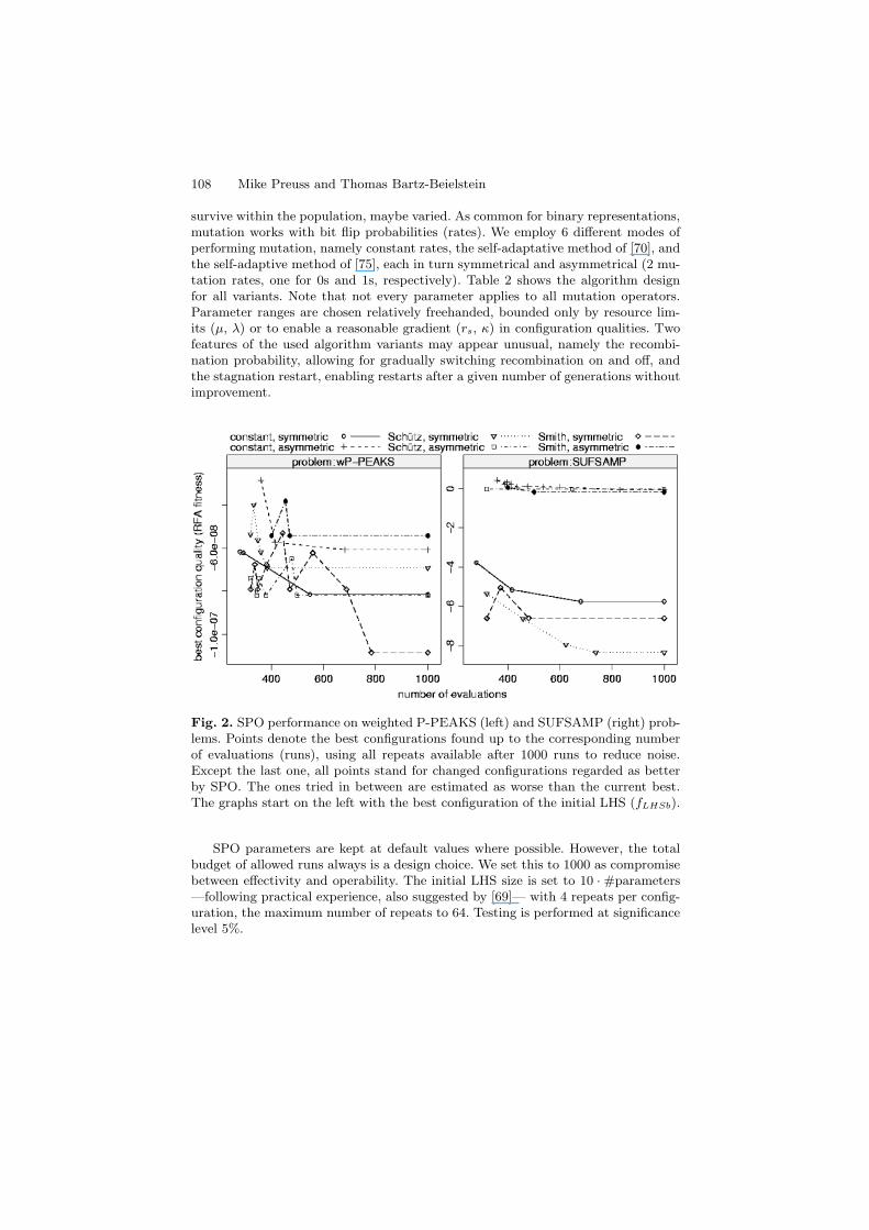
Fig. 2. SPO performance on weighted P-PEAKS (left) and SUFSAMP (right) prob-lems. Points denote the best configurations found up to the corresponding numberof evaluations (runs), using all repeats available after 1000 runs to reduce noise.Except the last one, all points stand for changed configurations regarded as betterby SPO. The ones tried in between are estimated as worse than the current best.The graphs start on the left with the best configuration of the initial LHS (fLHSb).

SPO parameters are kept at default values where possible. However, the totalbudget of allowed runs always is a design choice. We set this to 1000 as compromisebetween effectivity and operability. The initial LHS size is set to 10 · #parameters—following practical experience, also suggested by [69]— with 4 repeats per config-uration, the maximum number of repeats to 64. Testing is performed at significancelevel 5%.

SPO Applied to Self-Adaptation for Binary-Coded EAs 109

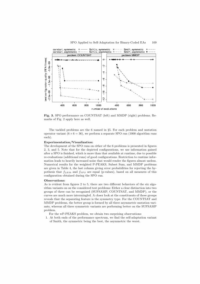
Fig. 3. SPO performance on COUNTSAT (left) and MMDP (right) problems. Re-marks of Fig. 2 apply here as well.

The tackled problems are the 6 named in §5. For each problem and mutationoperator variant (6× 6 = 36), we perform a separate SPO run (1000 algorithm runseach).

Experimentation/Visualization:The development of the SPO runs on either of the 6 problems is presented in figures2, 3, and 5. Note that for the depicted configurations, we use information gainedafter a SPO is finished, which is more than that available at runtime, due to possiblere-evaluations (additional runs) of good configurations. Restriction to runtime infor-mation leads to heavily increased noise that would render the figures almost useless.Numerical results for the weighted P-PEAKS, Subset Sum, and MMDP problemsare given in Table 4, the last column giving error probabilities for rejecting the hy-pothesis that fLHSb and fSPO are equal (p-values), based on all measures of thisconfiguration obtained during the SPO run.

Observations:As is evident from figures 2 to 5, there are two different behaviors of the six algo-rithm variants on on the considered test problems: Either a clear distinction into twogroups of three can be recognized (SUFSAMP, COUNTSAT, and MMDP), or thecurves are much more intermingled. A closer look at the constituents of these groupsreveals that the separating feature is the symmetry type. For the COUNTSAT andMMDP problems, the better group is formed by all three asymmetric mutation vari-ants, whereas all three symmetric variants are performing better on the SUFSAMPproblem.

For the wP-PEAKS problem, we obtain two surprising observations:1. At both ends of the performance spectrum, we find the self-adaptation variant

of Smith, the symmetric being the best, the asymmetric the worst.

110 Mike Preuss and Thomas Bartz-Beielstein

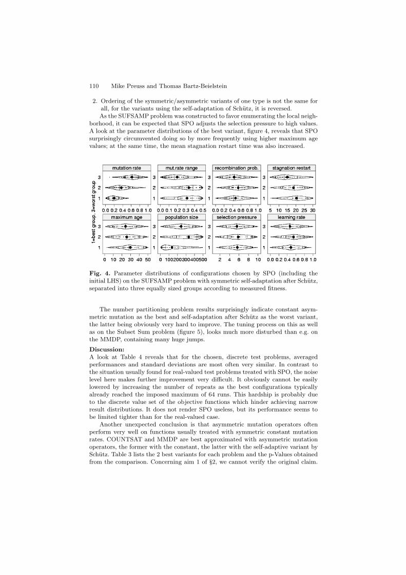
2. Ordering of the symmetric/asymmetric variants of one type is not the same forall, for the variants using the self-adaptation of Schutz, it is reversed.As the SUFSAMP problem was constructed to favor enumerating the local neigh-

borhood, it can be expected that SPO adjusts the selection pressure to high values.A look at the parameter distributions of the best variant, figure 4, reveals that SPOsurprisingly circumvented doing so by more frequently using higher maximum agevalues; at the same time, the mean stagnation restart time was also increased.

Fig. 4. Parameter distributions of configurations chosen by SPO (including theinitial LHS) on the SUFSAMP problem with symmetric self-adaptation after Schutz,separated into three equally sized groups according to measured fitness.

The number partitioning problem results surprisingly indicate constant asym-metric mutation as the best and self-adaptation after Schutz as the worst variant,the latter being obviously very hard to improve. The tuning process on this as wellas on the Subset Sum problem (figure 5), looks much more disturbed than e.g. onthe MMDP, containing many huge jumps.

Discussion:A look at Table 4 reveals that for the chosen, discrete test problems, averagedperformances and standard deviations are most often very similar. In contrast tothe situation usually found for real-valued test problems treated with SPO, the noiselevel here makes further improvement very difficult. It obviously cannot be easilylowered by increasing the number of repeats as the best configurations typicallyalready reached the imposed maximum of 64 runs. This hardship is probably dueto the discrete value set of the objective functions which hinder achieving narrowresult distributions. It does not render SPO useless, but its performance seems tobe limited tighter than for the real-valued case.

Another unexpected conclusion is that asymmetric mutation operators oftenperform very well on functions usually treated with symmetric constant mutationrates. COUNTSAT and MMDP are best approximated with asymmetric mutationoperators, the former with the constant, the latter with the self-adaptive variant bySchutz. Table 3 lists the 2 best variants for each problem and the p-Values obtainedfrom the comparison. Concerning aim 1 of §2, we cannot verify the original claim.

SPO Applied to Self-Adaptation for Binary-Coded EAs 111

Fig. 5. SPO performance on Number Partitioning (left) and Subset Sum (right).

There are problems for which self-adaptation is very useful, and there are somewhere it is not. Only in 2 of the six test cases, they have significant advantage.

Table 3. Bootstrap Permutation hypothesis tests between performances of the bestconstant and the best self-adaptive variant for each problem. The tests use all bestconfiguration runs available after SPO is finished, this is in most cases 64.

Problem Best Variant Second Variant p-Value Significant?

wP-PEAKS Smith, symmetric constant, symmetric 0.125 No

SUFSAMP Schutz, symmetric constant, symmetric 2e-05 Yes

COUNTSAT constant, asymmetric Schutz, asymmetric 0.261 No

MMDP Schutz, asymmetric constant, asymmetric 0.008 Yes

Number Part. constant, asymmetric Schutz, symmetric 0.489 No

Subset Sum constant, asymmetric Schutz, asymmetric 0.439 No

Concerning the effort needed for tuning constant and self-adaptive mutationoperators, we cannot account for a clear difference, thereby adhering to the originalclaim that tuning efforts are similar. However, there is neither statistical evidencein favor nor against this statement.

Nevertheless, when comparing the final best configurations to the average LHSresults, it becomes clear that without any tuning, algorithms may easily be miscon-figured, leading to performance values much worse than that of a simple EA-basedhillclimber. Moreover, the best point of an initial LHS appears as a reasonable es-timate for the quality achievable by tuning. Within this experiment, the LHS bestfitness fLHSb has always been superior to that of the (single-start) hillclimber.

112 Mike Preuss and Thomas Bartz-Beielstein

Is it possible to derive any connection between the properties of the tackledproblems and the success of different self-adaptation variants? We can detect simi-larities in the progression of the SPO runs, e.g. between COUNTSAT and MMDP,and Number Partitioning and Subset Sum, like the huge jumps found in case ofthe latter; these probably indicate result distributions much more complex than forthe former. However, it appears difficult to foresee if self-adaptation enhanced EAswill perform better or worse. In case of the MMDP, recombination is likely to pre-serve existing good blocks that may be optimized individually so that mutation rateschedules, once learned, can be successfully reapplied. But without further tests,this is rather speculation.

7 Conclusions

We motivated and explained the SPO procedure and, as a test case, applied it toself-adaptive EA variants for binary coded problems. This study revealed why self-adaptation is rarely applied for these problem types: It is hard to predict whether itwill increase performance, and which variant to choose. However, if properly para-metrized, it can be significantly faster than well tuned standard mutation operators.Modeling only a rough problem-mechanism interaction would require a much morethoroughly conducted study than presented here.

Surprisingly, specialized and seldomly used operators like the (constant and self-adaptive) asymmetric mutation performed very well when parametrized accordingly.This probably leads the way to superior operators still to develop—with or withoutself-adaptation. Mutation rate learning seems to provide rather limited potential.

The invented performance measures, RFA and AEB, were found capable of lead-ing the meta-search into the right direction. Unfortunately, the absence of well-defined measures for the tuning process itself currently prevents effectively usingSPO for answering questions concerning the tunability of an algorithm-problemcombination. This problem we want to tackle in future work.

Recapitulating, SPO works on binary problems, and proves to be a valuabletool for experimental analysis. However, there is room for improvement, first andforemost by taking measures to reduce the variances within the results of a singleconfiguration.

Acknowledgment

The research leading to this paper has been supported by the DFG (DeutscheForschungsgemeinschaft) as project no. 252441, “Mehrkriterielle Struktur- und Pa-rameteroptimierung verfahrenstechnischer Prozesse mit evolutionaren Algorithmenam Beispiel gewinnorientierter unscharfer destillativer Trennprozesse”. T. Bartz–Beielstein’s research was supported by the DFG as part of the collaborative researchcenter “Computational Intelligence” (531).

The autors want to thank Thomas Jansen for providing his code of the SUF-SAMP problem, and Silja Meyer-Nieberg and Nikolaus Hansen for sharing theiropinions with us.

Table

4.

Bes

tfo

und

configura

tion

per

form

ance

s,m

ean

valu

eofLH

S,bes

tofLH

S,and

bes

taft

erSP

Ois

finis

hed

,on

the

wei

ghte

dP

-P

EA

KS,Subse

tSum

,and

MM

DP

pro

ble

ms.

Bes

ides

the

RFA

fitn

essm

easu

reuse

dw

ithin

SP

O(t

om

inim

ize,

rela

tive

tohillc

lim

ber

),w

eals

ogiv

eth

eM

BF

and

AE

Bper

form

ance

mea

sure

s.A

EB

valu

esare

mea

nt

as

mult

iple

sof103.N

ote

that

wP

-PE

AK

Sand

MM

DP

(40)

are

tobe

maxim

ized

wit

hopti

malva

lues

at

1.0

and

40.0

,re

spec

tivel

y,and

Subse

tSum

isto

be

min

imiz

edto

0.0

.

Hillc

lim

ber

,f h

cLH

Sm

ean,f L

HS

aLH

Sbes

t,f L

HS

bSP

Obes

t,f S

PO

Adapta

tion

MB

FA

EB

RFA

stddev

MB

FA

EB

RFA

stddev

MB

FA

EB

RFA

stddev

MB

FA

EB

p-v

al

Pro

ble

m:w

P-P

EA

KS

none,

sym

0.9

45

<5

4.7

e-07

9.5

e-07

0.8

52

61.9

-6.2

e-08

6.7

e-08

0.9

84

52.1

-8.1

e-08

8.2

e-08

0.9

93

50.4

0.2

9

none,

asy

m0.9

45

<5

4.2

e-07

8.8

e-07

0.8

51

63.4

-2.9

e-08

8.3

e-08

0.9

64

48.8

-6.1

e-08

2.5

e-08

0.9

83

30.4

0.0

0

Sch

utz

,sy

m0.9

45

<5

5.0

e-07

9.1

e-07

0.8

44

60.5

-5.7

e-08

3.1

e-08

0.9

95

57.3

-6.9

e-08

1.1

e-07

0.9

80

46.2

0.4

6

Sch

utz

,asy

m0.9

45

<5

4.1

e-07

1.1

e-06

0.8

58

62.0

-7.4

e-08

8.2

e-08

0.9

84

48.3

-8.2

-08

4.4

e-08

0.9

84

24.2

0.3

5

Sm

ith,sy

m0.9

45

<5

4.9

e-07

1.0

e-06

0.8

46

58.5

-7.9

e-08

1.2

e-07

0.9

90

54.2

-1.1

e-07

1.6

e-07

0.9

87

46.1

0.1

2

Sm

ith,asy

m0.9

45

<5

4.0

e-07

8.6

e-07

0.8

58

63.1

-5.4

e-08

3.4

e-08

0.9

84

41.6

-5.4

e-08

3.4

e-08

0.9

84

41.6

0.5

0

Pro

ble

m:Subse

tSum

none,

sym

5.5

e+26

36.0

3.4

e+59

3.9

e+60

4.7

e+31

54.7

-7.3

e+48

1.2

e+49

1.6

e+26

49.3

-7.8

e+48

6.8

e+48

8.1

e+25

49.2

0.4

4

none,

asy

m5.5

e+26

36.0

1.4

e+59

6.4

e+59

3.2

e+31

52.5

-7.9

e+48

1.0

e+49

7.7

e+25

55.6

-1.1

e+49

1.6

e+49

7.7

e+25

38.0

0.1

8

Sch

utz

,sy

m5.5

e+26

36.0

1.9

e+59

1.1

e+60

5.0

e+31

53.9

-4.9

e+48

6.6

e+48

2.0

e+26

51.7

-7.7

e+48

5.6

e+48

4.3

e+25

51.2

0.0

4

Sch

utz

,asy

m5.5

e+26

36.0

2.5

e+59

1.9

e+60

2.9

e+31

49.4

-1.0

e+49

1.2

e+49

4.2

e+25

51.0

-1.1

e+49

1.4

e+49

7.1

e+25

48.1

0.4

2

Sm

ith,sy

m5.5

e+26

36.0

2.6

e+59

1.7

e+60

5.0

e+31

55.7

-5.1

e+48

5.2

e+48

1.3

e+26

58.3

-7.0

e+48

9.0

e+48

8.8

e+25

52.6

0.2

1

Sm

ith,asy

m5.5

e+26

36.0

3.2

e+59

4.5

e+60

2.8

e+31

51.1

-9.7

e+48

1.3

e+49

7.3

e+25

52.5

-9.7

e+48

1.3

e+49

7.3

e+25

52.5

0.5

0

Pro

ble

m:M

MD

P

none,

sym

23.8

058.1

-1.1

e-03

1.4

e-03

29.3

62.0

-4.3

e-03

2.3

e-03

37.0

54.3

-4.3

e-03

4.3

e-04

37.8

45.7

0.4

8

none,

asy

m23.8

058.1

-0.2

25

0.7

83

39.9

7.4

-4.6

04.8

340

<5

-7.1

311.7

40

<5

0.2

3

Sch

utz

,sy

m23.8

058.1

-1.3

e-03

1.7

e-03

30.0

63.0

-4.3

e-03

2.8

e-03

36.0

48.3

-4.6

e-03

2.3

e-03

37.6

54.3

0.3

7

Sch

utz

,asy

m23.8

058.1

-0.1

55

0.2

74

39.8

8.1

-2.2

80.8

94

40

<5

-12.0

10.9

40

<5

0.0

0

Sm

ith,sy

m23.8

058.1

-1.4

e-03

1.8

e-03

30.0

62.1

-4.1

e-03

2.4

e-03

37.3

59.6

-4.6

e-03

2.1

e-03

36.8

46.1

0.1

8

Sm

ith,asy

m23.8

058.1

-0.1

43

0.2

34

39.8

7.4

-1.5

60.7

74

40

<5

-8.4

16.5

940

<5

0.0

0

114 Mike Preuss and Thomas Bartz-Beielstein

References

1. Anne Auger and Nikolaus Hansen. Performance Evaluation of an AdvancedLocal Search Evolutionary Algorithm. In B. McKay et al., editors, Proc. 2005Congress on Evolutionary Computation (CEC’05), Piscataway NJ, 2005. IEEEPress.

2. T. Back. Evolutionary Algorithms in Theory and Practice. Oxford UniversityPress, New York NY, 1996.

3. T. Back and M. Schutz. Evolution strategies for mixed-integer optimization ofoptical multilayer systems. In J. R. McDonnell, R. G. Reynolds, and D. B.Fogel, editors, Evolutionary Programming IV: Proceedings of the Fourth AnnualConference on Evolutionary Programming, pages 33–51. MIT Press, Cambridge,MA, 1995.

4. Th. Back. Self-adaptation in genetic algorithms. In FJ Varela and P Bourgine,editors, Toward a Practice of Autonomous Systems: proceedings of the first Eu-ropean conference on Artificial Life, pages 263–271. MIT Press, 1992.

5. R. Barr and B. Hickman. Reporting computational experiments with parallelalgorithms: Issues, measures, and experts’ opinions. ORSA Journal on Comput-ing, 5(1):2–18, 1993.

6. Thomas Bartz-Beielstein. Evolution strategies and threshold selection. In M. J.Blesa Aguilera, C. Blum, A. Roli, and M. Sampels, editors, Proceedings SecondInternational Workshop Hybrid Metaheuristics (HM’05), volume 3636 of LectureNotes in Computer Science, pages 104–115, Berlin, Heidelberg, New York, 2005.Springer.

7. Thomas Bartz-Beielstein. Experimental Research in Evolutionary Computa-tion—The New Experimentalism. Springer, Berlin, Heidelberg, New York, 2006.

8. Thomas Bartz-Beielstein, Daniel Blum, and Jurgen Branke. Particle swarm op-timization and sequential sampling in noisy environments. In Richard Hartl andKarl Doerner, editors, Proceedings 6th Metaheuristics International Conference(MIC2005), pages 89–94, Vienna, Austria, 2005.

9. Thomas Bartz-Beielstein, Marcel de Vegt, Konstantinos E. Parsopoulos, andMichael N. Vrahatis. Designing particle swarm optimization with regressiontrees. Interner Bericht des Sonderforschungsbereichs 531 Computational Intel-ligence CI–173/04, Universitat Dortmund, Germany, Mai 2004.

10. Thomas Bartz-Beielstein, Christian Lasarczyk, and Mike Preuß. Sequential pa-rameter optimization. In B. McKay et al., editors, Proceedings 2005 Congresson Evolutionary Computation (CEC’05), Edinburgh, Scotland, volume 1, pages773–780, Piscataway NJ, 2005. IEEE Press.

11. Thomas Bartz-Beielstein and Boris Naujoks. Tuning multicriteria evolutionaryalgorithms for airfoil design optimization. Interner Bericht des Sonder-forschungsbereichs 531 Computational Intelligence CI–159/04, Universitat Dort-mund, Germany, Februar 2004.

12. Thomas Bartz-Beielstein, Konstantinos E. Parsopoulos, and Michael N.Vrahatis. Design and analysis of optimization algorithms using computa-tional statistics. Applied Numerical Analysis & Computational Mathematics(ANACM), 1(2):413–433, 2004.

13. Thomas Bartz-Beielstein, Mike Preuß, and Sandor Markon. Validation andoptimization of an elevator simulation model with modern search heuristics. In

SPO Applied to Self-Adaptation for Binary-Coded EAs 115

T. Ibaraki, K. Nonobe, and M. Yagiura, editors, Metaheuristics: Progress asReal Problem Solvers, Operations Research/Computer Science Interfaces, pages109–128. Springer, Berlin, Heidelberg, New York, 2005.

14. Regina Berretta, Carlos Cotta, and Pablo Moscato. Enhancing the performanceof memetic algorithms by using a matching-based recombination algorithm. InMetaheuristics: computer decision-making, pages 65–90. Kluwer Academic Pub-lishers, Norwell, MA, 2004.

15. Regina Berretta and Pablo Moscato. The number partitioning problem: an openchallenge for evolutionary computation? In New ideas in optimization, pages261–278. McGraw-Hill Ltd., Maidenhead, UK, 1999.

16. H.-G. Beyer and H.-P. Schwefel. Evolution strategies—A comprehensive intro-duction. Natural Computing, 1:3–52, 2002.

17. Marcel de Vegt. Einfluss verschiedener Parametrisierungen auf die Dynamikdes Partikel-Schwarm-Verfahrens: Eine empirische Analyse. Interner Berichtder Systems Analysis Research Group SYS–3/05, Universitat Dortmund, Fach-bereich Informatik, Germany, Dezember 2005.

18. Camil Demetrescu and Giuseppe F. Italiano. What do we learn from experi-mental algorithmics? In MFCS ’00: Proceedings of the 25th International Sym-posium on Mathematical Foundations of Computer Science, pages 36–51, Berlin,Heidelberg, New York, 2000. Springer.

19. N. R. Draper and H. Smith. Applied Regression Analysis. Wiley, New York NY,3rd edition, 1998.

20. S. Droste, T. Jansen, and I. Wegener. A natural and simple function which ishard for all evolutionary algorithms. In IEEE International Conference on In-dustrial Electronics, Control, and Instrumentation (IECON 2000), pages 2704–2709, Piscataway, NJ, 2000. IEEE Press.

21. A. E. Eiben, R. Hinterding, and Z. Michalewicz. Parameter control in evolution-ary algorithms. IEEE Transactions on Evolutionary Computation, 3(2):124–141,1999.

22. A. E. Eiben and J. E. Smith. Introduction to Evolutionary Computing. Springer,Berlin, Heidelberg, New York, 2003.

23. A.E. Eiben and M. Jelasity. A critical note on experimental research methodol-ogy in EC. In Proceedings of the 2002 Congress on Evolutionary Computation(CEC’2002), pages 582–587, Piscataway NJ, 2002. IEEE.

24. Robert Feldt and Peter Nordin. Using factorial experiments to evaluate the effectof genetic programming parameters. In Riccardo Poli et al., editors, GeneticProgramming, Proceedings of EuroGP’2000, volume 1802 of Lecture Notes inComputer Science, pages 271–282, Berlin, Heidelberg, New York, 15-16 April2000. Springer.

25. D. B. Fogel. Evolving Artificial Intelligence. PhD thesis, University of California,San Diego, 1992.

26. O. Francois and C. Lavergne. Design of evolutionary algorithms—a statisticalperspective. IEEE Transactions on Evolutionary Computation, 5(2):129–148,April 2001.

27. Mario Giacobini, Mike Preuß, and Marco Tomassini. Effects of scale-free andsmall-world topologies on binary coded self-adaptive CEA. In 6th EuropeanConf. Evolutionary Computation in Combinatorial Optimization, Proc. (Evo-COP’06), Lecture Notes in Computer Science, pages 86–98, Berlin, 2006.Springer.

116 Mike Preuss and Thomas Bartz-Beielstein

28. D. E. Goldberg, K. Deb, and J. Horn. Massively multimodality, deception andgenetic algorithms. In R. Manner and B. Manderick, editors, Parallel Prob.Solving from Nature II, pages 37–46. North-Holland, 1992.

29. Garrison W. Greenwood. Adapting mutations in genetic algorithms using geneflow principles. In R. Sarker et al., editors, Proc. 2003 Congress on Evolution-ary Computation (CEC’03), Canberra, pages 1392–1397, Piscataway NJ, 2003.IEEE Press.

30. N. Hansen and A. Ostermeier. Completely derandomized self-adaptation inevolution strategies. Evolutionary Computation, 9(2):159–195, 2001.

31. N. Hansen, A. Ostermeier, and A. Gawelczyk. On the adaptation of arbitrarynormal mutation distributions in evolution strategies: The generating set adap-tation. In L. J. Eshelman, editor, Proc. 6th Int’l Conf. on Genetic Algorithms,pages 57–64, San Francisco, CA, 1995. Morgan Kaufmann Publishers, Inc.

32. J. Hooker. Testing heuristics: We have it all wrong. Journal of Heuristics,1(1):33–42, 1996.

33. Christian Igel and Martin Kreutz. Operator adaptation in evolutionary compu-tation and its application to structure optimization of neural networks. Neuro-computing, 55(1-2):347–361, 2003.

34. E. H. Isaaks and R. M. Srivastava. An Introduction to Applied Geostatistics.Oxford University Press, Oxford, U.K., 1989.

35. Thomas Jansen, Kenneth A. De Jong, and Ingo Wegener. On the choice of theoffspring population size in evolutionary algorithms. Evolutionary Computation,13(4):413–440, 2005.

36. Thomas Jansen and Dirk Sudholt. Design and analysis of an asymmetric muta-tion operator. In B. McKay et al., editors, Proc. 2005 Congress on EvolutionaryComputation (CEC’05), Edinburgh, Scotland, volume 1, pages 190–197, Piscat-away NJ, 2005. IEEE Press.

37. Mark Jelasity. A wave analysis of the subset sum problem. In Thomas Back, ed-itor, Proceedings of the Seventh International Conference on Genetic Algorithms(ICGA97), pages 89–96, San Francisco, CA, 1997. Morgan Kaufmann.

38. Mark Jelasity, Mike Preuß, and Agoston E. Eiben. Operator learning for a prob-lem class in a distributed peer-to-peer environment. In J. J. Merelo Guervos,P. Adamidis, H.-G. Beyer, J.L. Fernandez-Villacanas, and H.-P. Schwefel, ed-itors, Parallel Problem Solving from Nature – PPSN VII, Proc. Seventh Int’lConf., Granada, pages 172–183, Berlin, 2002. Springer.

39. David S. Johnson. A theoretician’s guide to the experimental analysis of al-gorithms. In M. H. Goldwasser, D. S. Johnson, and C. C. McGeoch, editors,Data Structures, Near Neighbor Searches, and Methodology: Fifth and Sixth DI-MACS Implementation Challenges, pages 215–250, Providence, 2002. AmericanMathematical Society.

40. D.R. Jones, M. Schonlau, and W.J. Welch. Efficient global optimization of ex-pensive black-box functions. Journal of Global Optimization, 13:455–492, 1998.

41. Kenneth A. De Jong, Michael A. Potter, and William M. Spears. Using problemgenerators to explore the effects of epistasis. In T. Back, editor, Proceedings ofthe Seventh ICGA, pages 338–345. Morgan Kaufmann, 1997.

42. Bryant A. Julstrom. Adaptive operator probabilities in a genetic algorithm thatapplies three operators. In SAC ’97: Proceedings of the 1997 ACM symposiumon Applied computing, pages 233–238, New York, NY, 1997. ACM Press.

43. J. P. C. Kleijnen. Statistical Tools for Simulation Practitioners. Marcel Dekker,New York NY, 1987.

SPO Applied to Self-Adaptation for Binary-Coded EAs 117

44. J. P. C. Kleijnen. Experimental design for sensitivity analysis, optimization, andvalidation of simulation models. In J. Banks, editor, Handbook of Simulation.Wiley, New York NY, 1997.

45. F. Kursawe. Grundlegende empirische Untersuchungen der Parameter vonEvolutionsstrategien – Metastrategien. Dissertation, Fachbereich Informatik,Universitat Dortmund, Germany, 1999.

46. A.M. Law and W.D. Kelton. Simulation Modeling and Analysis. McGraw-Hill,New York NY, 3rd edition, 2000.

47. S.N. Lophaven, H.B. Nielsen, and J. Søndergaard. Aspects of the Matlab Tool-box DACE. Technical Report IMM-REP-2002-13, Informatics and Mathemati-cal Modelling, Technical University of Denmark, Copenhagen, Denmark, 2002.

48. S.N. Lophaven, H.B. Nielsen, and J. Søndergaard. DACE—A Matlab KrigingToolbox. Technical Report IMM-REP-2002-12, Informatics and MathematicalModelling, Technical University of Denmark, Copenhagen, Denmark, 2002.

49. Sandor Markon, Hajime Kita, Hiroshi Kise, and Thomas Bartz-Beielstein, edi-tors. Modern Supervisory and Optimal Control with Applications in the Controlof Passenger Traffic Systems in Buildings. Springer, Berlin, Heidelberg, NewYork, 2006.

50. Catherine C. McGeoch. Experimental Analysis of Algorithms. PhD thesis,Carnegie Mellon University, Pittsburgh PA, 1986.

51. M. D. McKay, R. J. Beckman, and W. J. Conover. A comparison of threemethods for selecting values of input variables in the analysis of output from acomputer code. Technometrics, 21(2):239–245, 1979.

52. Jorn Mehnen, Thomas Michelitsch, Thomas Bartz-Beielstein, and NadineHenkenjohann. Systematic analyses of multi-objective evolutionary algorithmsapplied to real-world problems using statistical design of experiments. In R. Teti,editor, Proceedings Fourth International Seminar Intelligent Computation inManufacturing Engineering (CIRP ICME’04), volume 4, pages 171–178, Naples,Italy, 2004.

53. Jorn Mehnen, Thomas Michelitsch, Thomas Bartz-Beielstein, and Chris-tian W. G. Lasarczyk. Multiobjective evolutionary design of mold temperaturecontrol using DACE for parameter optimization. In H. Pfutzner and E. Leiss,editors, Proceedings Twelfth International Symposium Interdisciplinary Electro-magnetics, Mechanics, and Biomedical Problems (ISEM 2005), volume L11-1,pages 464–465, Vienna, Austria, 2005. Vienna Magnetics Group Reports.

54. Silja Meyer-Nieberg and Hans-Georg Beyer. Self-adaptation in evolutionaryalgorithms. In Fernando Lobo, Claudio Lima, and Zbigniew Michalewicz, edi-tors, Parameter Setting in Evolutionary Algorithms, Studies in ComputationalIntelligence. Springer, Berlin Heidelberg New York, 2006.

55. D. C. Montgomery. Design and Analysis of Experiments. Wiley, New York NY,5th edition, 2001.

56. B. M. E. Moret. Towards a discipline of experimental algorithmics. In M.H.Goldwasser, D.S. Johnson, and C.C. McGeoch, editors, Data Structures, NearNeighbor Searches, and Methodology: Fifth and Sixth DIMACS Implementa-tion Challenges, DIMACS Monographs 59 , pages 197–213, Providence RI, 2002.American Mathematical Society.

57. Bernard M. Moret and Henry D. Shapiro. Algorithms and experiments: The new(and old) methodology. Journal of Universal Computer Science, 7(5):434–446,2001.

118 Mike Preuss and Thomas Bartz-Beielstein

58. R. Myers and E.R. Hancock. Empirical modelling of genetic algorithms. Evo-lutionary Computation, 9(4):461–493, 2001.

59. Martin Pelikan, David E. Goldberg, and Erick Cantu-Paz. Linkage problem,distribution estimation, and bayesian networks. Evolutionary Computation,8(3):311–340, 2000.

60. F. Pukelsheim. Optimal Design of Experiments. Wiley, New York NY, 1993.61. Iloneide C. O. Ramos, Marco C. Goldbarg, Elizabeth G. Goldbarg, and Adriao

D. Doria Neto. Logistic Regression for Parameter Tuning on an EvolutionaryAlgorithm. In B. McKay et al., editors, Proc. 2005 Congress on EvolutionaryComputation (CEC’05), volume 2, pages 1061–1068, Piscataway NJ, 2005. IEEEPress.

62. Ronald L. Rardin and Reha Uzsoy. Experimental evaluation of heuristic opti-mization algorithms: A tutorial. J. Heuristics, 7(3):261–304, 2001.

63. I. Rechenberg. Evolutionsstrategie: Optimierung technischer Systeme nachPrinzipien der biologischen Evolution. Frommann-Holzboog Verlag, Stuttgart,1973.

64. I. Rechenberg. Evolutionsstrategien. In B. Schneider and U. Ranft, editors, Sim-ulationsmethoden in der Medizin und Biologie, pages 83–114. Springer-Verlag,Berlin, 1978.

65. J. Sacks, W. J. Welch, T. J. Mitchell, and H. P. Wynn. Design and analysis ofcomputer experiments. Statistical Science, 4(4):409–435, 1989.

66. T. J. Santner, B. J. Williams, and W. I. Notz. The Design and Analysis ofComputer Experiments. Springer, Berlin, Heidelberg, New York, 2003.

67. J. D. Schaffer, R. A. Caruana, L. Eshelman, and R. Das. A study of con-trol parameters affecting online performance of genetic algorithms for functionoptimization. In J. D. Schaffer, editor, Proceedings of the Third InternationalConference on Genetic Algorithms, pages 51–60, San Mateo CA, 1989. MorganKaufman.

68. M. Schonlau. Computer Experiments and Global Optimization. PhD thesis,University of Waterloo, Ontario, Canada, 1997.

69. Matthias Schonlau, William J. Welch, and Ronald R. Jones. Global versus localsearch in constrained optimization of computer models. In New Developmentand Applications in Experimental Design, number 34 in IMS Lecture Notes,pages 11–25. Institute of Mathematical Statistics, Beachwood, OH, 1998.

70. Martin Schutz. Eine Evolutionsstrategie fur gemischt-ganzzahlige Optimier-probleme mit variabler Dimension. Interner Bericht der Systems Analysis Re-search Group SYS–1/96, Universitat Dortmund, Fachbereich Informatik, Au-gust 1996.

71. H.-P. Schwefel. Adaptive Mechanismen in der biologischen Evolution und ihrEinfluß auf die Evolutionsgeschwindigkeit. Technical report, Technical Univer-sity of Berlin, 1974. Abschlußbericht zum DFG-Vorhaben Re 215/2.

72. H.-P. Schwefel. Numerical Optimization of Computer Models. Wiley, Chichester,1981.

73. H.-P. Schwefel, I. Wegener, and K. Weinert, editors. Advances in Computa-tional Intelligence—Theory and Practice. Springer, Berlin, Heidelberg, NewYork, 2003.

74. J. Smith and T. C. Fogarty. Self-adaptation of mutation rates in a steady stategenetic algorithm. In Proceedings of 1996 IEEE Int’l Conf. on EvolutionaryComputation (ICEC ’96), pages 318–323. IEEE Press, NY, 1996.

SPO Applied to Self-Adaptation for Binary-Coded EAs 119

75. J. E. Smith. Modelling gas with self adaptive mutation rates. In L. Spectorand et al., editors, Proceedings of the Genetic and Evolutionary ComputationConference (GECCO-2001), pages 599–606, San Francisco, California, USA, 7-11 July 2001. Morgan Kaufmann.

76. Catalin Stoean, Mike Preuss, Ruxandra Gorunescu, and Dan Dumitrescu. ElitistGenerational Genetic Chromodynamics - a New Radii-Based Evolutionary Al-gorithm for Multimodal Optimization. In B. McKay et al., editors, Proc. 2005Congress on Evolutionary Computation (CEC’05), volume 2, pages 1839 – 1846,Piscataway NJ, 2005. IEEE Press.

77. Ch. Stone and J. E. Smith. Strategy parameter variety in self-adaptation ofmutation rates. In W. B. Langdon and et al., editors, GECCO, pages 586–593.Morgan Kaufmann, 2002.

78. Dirk Thierens. An adaptive pursuit strategy for allocating operator proba-bilities. In GECCO ’05: Proceedings of the 2005 conference on Genetic andevolutionary computation, pages 1539–1546, New York, NY, 2005. ACM Press.

79. Marko Tosic. Evolutionare Kreuzungsminimierung. Diploma thesis, Universityof Dortmund, Germany, January 2006.

80. Klaus Weinert, Jorn Mehnen, Thomas Michelitsch, Karlheinz Schmitt, andThomas Bartz-Beielstein. A multiobjective approach to optimize temperaturecontrol systems of moulding tools. Production Engineering Research and Devel-opment, Annals of the German Academic Society for Production Engineering,XI(1):77–80, 2004.

81. Darrell Whitley, Soraya B. Rana, John Dzubera, and Keith E. Mathias. Evalu-ating evolutionary algorithms. Artificial Intelligence, 85(1-2):245–276, 1996.

82. D.H. Wolpert and W.G. Macready. No free lunch theorems for optimization.IEEE Transactions on Evolutionary Computation, 1(1):67–82, 1997.