Hybrid FE/ANN and LPR approach for the inverseidentification of material parameters from cutting tests

Ana Muñoz-Sánchez & Isabel M. González-Farias &

Xavier Soldani & M. Henar Miguélez

Abstract Accuracy of numerical models based in finiteelements (FE), extensively used for simulation of cuttingprocesses, depends strongly on the identification of propermaterial parameters. Experimental identification of theconstitutive law parameters for simulation of cuttingprocesses involves unsolved problems such as the complextesting techniques or the difficulty to reproduce the stresstriaxiality state during cutting. This work proposes amethodology for the inverse identification of the materialparameters from cutting test. Two hybrid approaches arecompared. One of them based on FE and artificial neuralnetworks (ANN). The other one based on FE and localpolynomial regression (LPR). Firstly, a FE model isvalidated with experimental data. Then, ANN and LPRare trained with FE simulations. Finally, the estimated ANNand LPR models are used for the inverse identification ofmaterial parameters. This identification is solved as anoptimization problem. The FE/LPR approach shows goodperformance, outperforming the FE/ANN approach.

Keywords Inverse technique . Cutting simulation . FE .

ANN . Local polynomial regression

NomenclatureParameters of constitutive equationσY Equivalent stressA Yield limitB Strain hardening coefficient

n Strain hardening exponentC Strain rate hardening coefficientm Thermal softening coefficientεpl Equivalent plastic strain�"pl Equivalent plastic strain rate�"0 Reference strain rateθ Temperatureθref Reference temperatureθmelt Melting temperature

Description of the methodologyμ Friction coefficient at the interfaceFc Cutting forceFt Thrust forceσ11 Tensile residual stresses at

machined surface in direction 1σ33 Tensile residual stresses at

machined surface in direction 3A(i), B(i), n(i) Random values being the input

variables of RBFN or LPRbFcðiÞ; bFtðiÞ; bs11ðiÞ; bs33ðiÞ Estimated values of forces andresidual stress

RBFN and LPR modelsX ¼ X1;X2; :::;Xp

� �0Predictor input variables

Y Response variable

RBFNK(•) Univariate kernel function||•|| Euclidean distanceJ Number of hidden unitsvj Output of the j-th hidden unitCj Vector of centres of the j-th hidden unitTj Width of the kernel functionbY Estimated value of response variablew0k wjk Weights associated with the output unit k

A. Muñoz-Sánchez : I. M. González-Farias :X. Soldani :M. H. Miguélez (*)Department of Mechanical Engineering,Universidad Carlos III de Madrid,Av. de la Universidad 30,28911 Leganés, Madrid, Spaine-mail: mhmiguel@ing.uc3m.es

1

LPRxi; yif g; i ¼ 1; 2; . . . ; n Sample observations

wi Weight for the ith observationβj Regression coefficientd Grade of the polynomialhj Bandwidth (smoothing parameter)Kh (uj) Univariate kernel for the

variable Xj

KH Kernel function product ofunivariate kernels

Models estimationM Number of iterationsN Number of observations of the datasetNv Validation observationss Number of output variablesy Real valueby Estimated valueMARE Mean absolute relative errorMSE Mean square errorAPE Absolute percentage errorMAPE Mean absolute percentage error

1 Introduction

Manufacturing processes should ensure not only competi-tive time and cost production, but also the development ofcomponents with high quality, especially in the case of highresponsibility applications. Simulation tools are widelyused in all steps of product design, not only for structuralcalculations, also for processing route design, being thisstep related with final service behaviour of the component.Numerical models based on finite elements (FE) have beenextensively used for machining simulation [1, 2], howevermany aspects related with numerical simulations remainunsolved.

The identification of material parameters for cuttingsimulation, strongly influent in the numerical results, is anobjective that should be achieved. Many problems remainunsolved when a representative constitutive law should bestated. Firstly, the inexistence of experimental tests able toreproduce the special conditions involved during cutting.Current characterization tests induce stress states in thespecimen quite different from those obtained duringmachining. Another problem is performing typical tests athigh strain rates (for instance using metallic sheets in tensiletests) for the same material treatment and the same formatas used in machining tests (as an example, bars in turningoperations). The work path suffered in different manufactureprocess leads to different mechanical properties. Differentworks in scientific literature show reasonable doubts relatedwith the convenience of applying constitutive equation

parameters obtained in traditional test to simulate cuttingprocesses. The best solution could be using machining tests toidentify the constitutive equation parameters [3].

Artificial neural networks (ANN) and local polynomialregression (LPR) techniques could help in the identificationof constitutive law parameters for specific machiningconditions. These nonparametric techniques require noassumptions about the form of the relationship between aset of variables.

Hence, they are particularly useful when little informationabout the model structure is available.

ANN have been extensively used in a wide variety ofapplications related with manufacturing processes (see forinstance [4–6]).

On the other hand LPR techniques [7] have not beencommonly used for the analysis of manufacturing processes.These statistical tool provide similar characteristics andrequirements as ANN to threat complex relationships, withlittle information about the interdependence of the input andoutput variables, however their use has been limited to otherfields.

Despite of the potentiality of ANN and LPR models, themain drawback of these techniques is the requirement of alarge amount of data for training process. In our context, itis really difficult to have a large amount of experimentaldata. The variety of materials that should be involved toreproduce a wide range of variation of constitutiveparameters would be extremely high. Furthermore, it isnot possible to control the constitutive parameters of thematerials tested. Thus, the use of validated FE models is analternative way to generate numerical data to find the bestANN and LPR models.

The hybrid FE/ANN approach has been used in differentanalysis of manufacturing processes and other fields. Forinstance, Umbrello et al. [8] used this combined method topredict machining induced residual stresses during hardturning; and Chamekh et al. [9] proposed a hybridprocedure for the identification of HILL anisotropicparameters based on deep drawing of a cylindrical cup.Fernández-Fdz and Zaera [10] used the combined approachto predict the penetration behaviour of ceramic targetsunder the impact of different projectiles.

In this work, we propose a hybrid procedure for theinverse identification of material parameters from cuttingtests. The aim is obtaining constitutive equation parameterssuitable to be implemented in FE codes for accuratesimulation of cutting. Two approaches, one based FE/ANN and the other one based on FE/LPR are compared inorder to find the best hybrid procedure. These approachesare based on the following variables: (1) the forces and thefriction coefficient at the interface, measured/estimatedduring cutting tests. (2) The machining induced residualstresses, measured on the machined surface. These variables

2

are highly sensible to variations of the material parameters.Residual stresses were selected because of both its depen-dence on material parameters and due to their relevance assurface integrity indicators [11].

Thus, the methodology proposed in this work relatesexperimental data obtained from orthogonal cutting testsand subsequent measurements on the machined workpiece,with the values of the parameters of the constitutiveequation. This approach could simplify significantly theexperimental devices needed for research in this field.

The proposed FE/ANN and FE/LPR approaches aredivided in three different stages. In the first stage, a FEmodel is developed using experimental data. Then, thevalidated model is used to perform a great number ofsimulations, changing the input data and obtaining a widerange of cutting forces and level of residual stresses for thedifferent ranges of material parameters covered. In thesecond stage, both ANN and LPR models are trained byusing a large set of numerical results obtained from FEmodel. The neural network used is the Radial BasisFunction Network (RBFN). Finally, the last stageinvolves the inverse identification procedure. In thisstage the objective is the prediction of the constitutiveparameters according to specific values of cutting forcesand residual stresses obtained from cutting tests. Theidentification problem is solved as an optimizationproblem using the estimated RBFN and LPR modelsfrom second stage.

The rest of the article is organized as follows. Section 2describes the steps of the proposed FE/ANN and FE/LPRprocedures. Section 3 describes the FE model and itsexperimental validation. Theoretical concepts related withRBFN and LPR techniques are briefly explained in sectionfourth. Sections 5 shows the results, and finally section 6summarizes the conclusions of the work.

2 Methodology

The methodology is illustrated in Fig. 1. At the first stage(corresponding with the upper box of Fig. 1), the FE model,able to predict both cutting forces and residual stresses, wasdeveloped and validated with experimental data. TheJonhson-Cook [12] constitutive law (see Eq. 1) was usedin this work due to its ability to simulate mechanicalprocesses involving high strain and strain rate and thermalsoftening. This constitutive law is commonly used insimulations of cutting processes [13].

sY ¼ Aþ B "pl� �n� � � 1þ C ln

�"pl�"

� �� �� 1� q � qref

qmelt � qref

� �m� �ð1Þ

being σY, equivalent stress; A, yield limit; B, strainhardening coefficient; n, strain hardening exponent; C,strain rate hardening coefficient; m, thermal softeningcoefficient; εpl, equivalent plastic strain; �"pl, equivalentplastic strain rate; �"0, reference strain rate; θ, temperature;θref, reference temperature; and θmelt, melting temperature.

Cutting tests of AISI 316L were used for the validation ofthe FEmodel. This alloy is similar (mechanical behaviour andphysical properties) to those materials that will be studied inthe last section of the paper. The experimentally validated FEmodel was used to generate a large dataset for the secondstage. This data set was obtained by varying the parameters ofconstitutive equation, A, B and n; and the friction coefficientat the interface, μ. The output variables were the cutting andthrust force, Fc, and Ft, and the level of tensile residualstresses in machined surface in direction 1, σ11, and indirection 3, σ33. (see Fig. 2). These directions correspond,respectively, with circumferential and axial directions of theorthogonal cutting tests performed to validate the FE model.Cutting forces are significant parameters related with themechanical behaviour of the workpiece material, and theyare relatively easy to measure during machining tests.Residual stresses in machined surface, which should bemeasured in a post mortem analysis of the machinedspecimen, are related with both mechanical and thermalphenomena during cutting. The sensibility of residual stressto variations of constitutive parameters A, B and n, havebeen analyzed recently in scientific literature [14]. Also theterms of the constitutive equation related with strain ratesensitivity and thermal softening (C and m, respectively)could influence the residual stresses and the cuttingforces. However, the prediction of these parameterswould involve a large number of simulations. Thus, despiteof the interest of a full approach involving all terms ofconstitutive equation (strain hardening, strain rate hardeningand thermal softening) this work is restricted to the threecoefficients A, B, n.

At the second stage (corresponding with intermediatebox of Fig. 1, see also Fig. 3) RBF and LPR models areestimated by using the dataset from FE model. The inputand output variables of these models are the same usedin FE model. That is, the input variables are theparameters A, B and μ, and the output variables were Fc,Ft, σ11 and σ33.

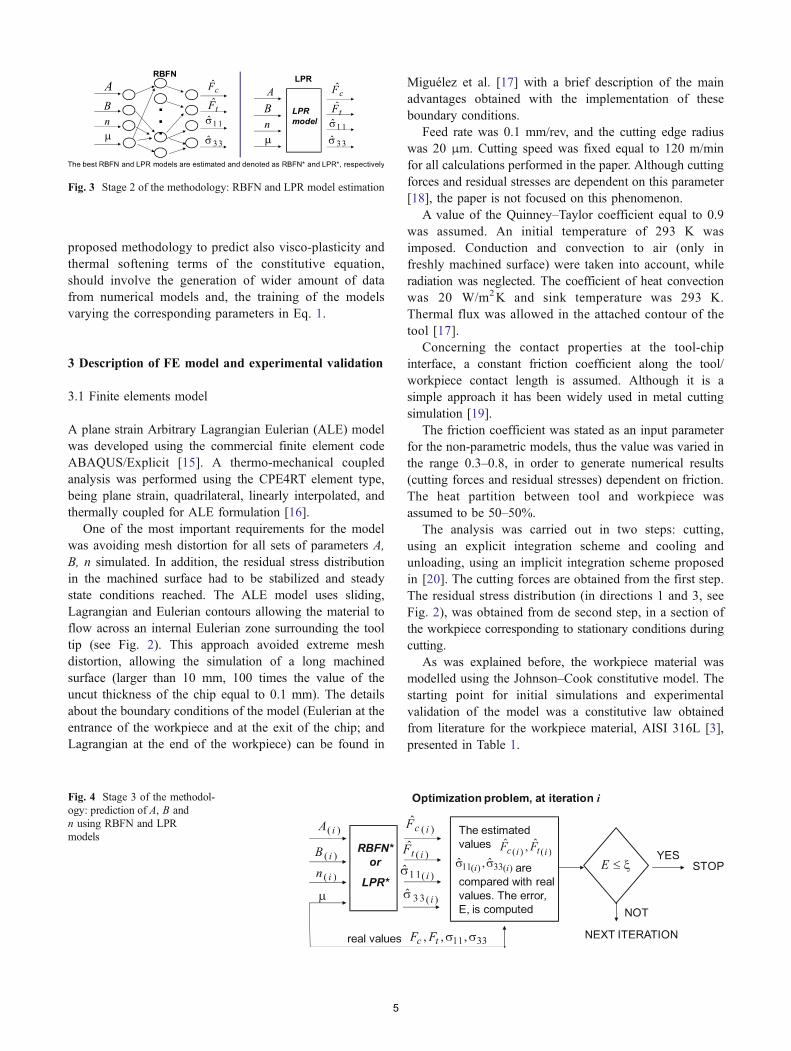
Finally, at the third stage (lowest box in Fig. 1, see alsoFig. 4) the inverse identification is performed. During thisstage, an optimization problem was solved. Now theinput variables are a set of specific values of Fc, Ft, σ11,σ33 and μ. The objective is to find the values of A, B and naccording those input values. The estimated RBFN andLPR models of the second stage are used to related inputand output variables. At the iteration i of the optimizationproblem, a set of random values A(i), B(i) and n(i) along

3

with the value μ are the input variables of RBFN or LPRmodels. For these values, the corresponding bFcðiÞ; bFtðiÞ;bs11ðiÞ and bs33ðiÞare estimated. The values A(i), B(i) and n(i)that minimize the difference between bFcðiÞ; bFtðiÞ; bs11ðiÞ andbs33ðiÞ and Fc, Ft, σ11, σ33, are the predicted constitutivematerial parameters.

Concerning the limitations of the method proposed, itshould be noted that the RBFN and LPR models couldbe used to predict parameters A, B and n, correspondingto materials showing thermal softening and strain ratehardening behaviour similar to those used during thetraining process of the models. Further application of the

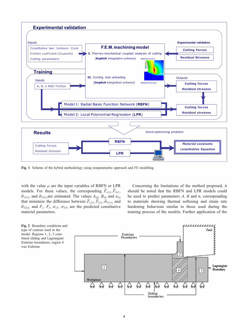
Fig. 1 Scheme of the hybrid methodology using nonparametric approach and FE modelling

Fig. 2 Boundary conditions andtype of contour used in themodel. Regions 1, 2, 3 com-bined sliding and Lagrangian/Eulerian boundaries; region 4was Eulerian

4

proposed methodology to predict also visco-plasticity andthermal softening terms of the constitutive equation,should involve the generation of wider amount of datafrom numerical models and, the training of the modelsvarying the corresponding parameters in Eq. 1.

3 Description of FE model and experimental validation

3.1 Finite elements model

A plane strain Arbitrary Lagrangian Eulerian (ALE) modelwas developed using the commercial finite element codeABAQUS/Explicit [15]. A thermo-mechanical coupledanalysis was performed using the CPE4RT element type,being plane strain, quadrilateral, linearly interpolated, andthermally coupled for ALE formulation [16].

One of the most important requirements for the modelwas avoiding mesh distortion for all sets of parameters A,B, n simulated. In addition, the residual stress distributionin the machined surface had to be stabilized and steadystate conditions reached. The ALE model uses sliding,Lagrangian and Eulerian contours allowing the material toflow across an internal Eulerian zone surrounding the tooltip (see Fig. 2). This approach avoided extreme meshdistortion, allowing the simulation of a long machinedsurface (larger than 10 mm, 100 times the value of theuncut thickness of the chip equal to 0.1 mm). The detailsabout the boundary conditions of the model (Eulerian at theentrance of the workpiece and at the exit of the chip; andLagrangian at the end of the workpiece) can be found in

Miguélez et al. [17] with a brief description of the mainadvantages obtained with the implementation of theseboundary conditions.

Feed rate was 0.1 mm/rev, and the cutting edge radiuswas 20 μm. Cutting speed was fixed equal to 120 m/minfor all calculations performed in the paper. Although cuttingforces and residual stresses are dependent on this parameter[18], the paper is not focused on this phenomenon.

A value of the Quinney–Taylor coefficient equal to 0.9was assumed. An initial temperature of 293 K wasimposed. Conduction and convection to air (only infreshly machined surface) were taken into account, whileradiation was neglected. The coefficient of heat convectionwas 20 W/m2K and sink temperature was 293 K.Thermal flux was allowed in the attached contour of thetool [17].

Concerning the contact properties at the tool-chipinterface, a constant friction coefficient along the tool/workpiece contact length is assumed. Although it is asimple approach it has been widely used in metal cuttingsimulation [19].

The friction coefficient was stated as an input parameterfor the non-parametric models, thus the value was varied inthe range 0.3–0.8, in order to generate numerical results(cutting forces and residual stresses) dependent on friction.The heat partition between tool and workpiece wasassumed to be 50–50%.

The analysis was carried out in two steps: cutting,using an explicit integration scheme and cooling andunloading, using an implicit integration scheme proposedin [20]. The cutting forces are obtained from the first step.The residual stress distribution (in directions 1 and 3, seeFig. 2), was obtained from de second step, in a section ofthe workpiece corresponding to stationary conditions duringcutting.

As was explained before, the workpiece material wasmodelled using the Johnson–Cook constitutive model. Thestarting point for initial simulations and experimentalvalidation of the model was a constitutive law obtainedfrom literature for the workpiece material, AISI 316L [3],presented in Table 1.

Fig. 3 Stage 2 of the methodology: RBFN and LPR model estimation

Fig. 4 Stage 3 of the methodol-ogy: prediction of A, B andn using RBFN and LPRmodels

5

Physical properties of cutting material (carbide) andworkpiece material were obtained from scientific literature(references [14, 21]) and are presented in Tables 2 and 3.

3.2 Experimental validation

The model was validated with experimental data obtainedfrom orthogonal cutting tests (AISI316L) and subsequentmeasurement of residual stresses in the machined surface.The value of the friction coefficient equal to 0.4 reproducedaccurately the resultant residual stresses observed inexperimental tests performed in the laboratory.

Orthogonal dry cutting tests with air cooling werecarried out in a lathe (PINACHO model Smart-Turn 6/165) with the following parameters: cutting speed 120 m/min, feed rate 0.1 mm/rev, depth of cut equal to 2 mm. Theworkpiece material was a tube of AISI 316L steel with awall thickness equal to 2 mm.

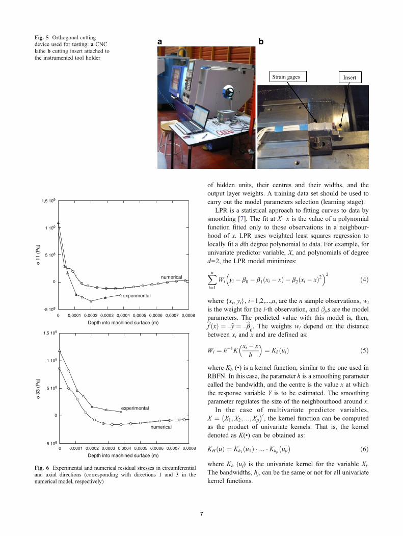
The tool geometry was generated by electro-dischargemachining in a hard metal preform. Cutting edge radius was20 μm. The rake angle and the clearance angle wererespectively 0° and 5°, obtained by positioning the insert inthe tool holder. The support of the tool was instrumentedwith strain gauges allowing measurement of the cuttingforce during orthogonal cutting of the tube (see Fig. 5). Thecutting edge of the insert was located coaxially with theaxis of the support, avoiding the effect of torque duringcutting. Cutting and trust forces predicted with numericalmodel matched reasonably the values measured in thecutting tests in the lathe. Errors below 15% were obtainedfor cutting force prediction. However, the model does notpredict accurately thrust force. As is well known, theinaccuracy in predicting thrust force is a common problemof FE cutting models.

The distribution of residual stress in circumferentialdirection was measured in the Technological CentreIDEKO (see http://www.ideko.es). The in depth distributionof residual stresses, both in circumferential and axialdirections, were approximately predicted with the model

(see Fig. 6). Experimental tensile value in the machinedsurface is larger than predicted value (error around 20%).This behaviour could be related with the effect of theprevious cut that appears in the turning tests. In theexperimental tests used to validate simulations, the maincutting edge cuts the machined surface generated in theprevious revolution of the lathe. In the case of difficult tocut material like AISI 316L, this zone is strongly affectedby the previous cut [22] increasing the induced residualstresses in the workpiece. This increment could explain thedifferences observed between predicted and measuredresidual stresses.

4 Theoretical concepts of RBFN and LPR

The RBFN and LPR are nonparametric techniques toestimate the conditional expectation of a response variable,Y, given a set of p predictor variables X ¼ X1;X2; :::;Xp

� �0.

RBFN is a feed-forward network with three layers:input, hidden and output layer [23]. The input layer iscomposed of the input variables, X. The hidden layer of Junits transforms the data from the input space by applying akernel function, K(•). The output vj of the jth hidden unit isobtained as:

vj ¼ KX� Cj

�� ��Tj

� �ð2Þ

where Cj is the vector of centres, Tj controls the width ofthe kernel function and ||•|| denotes the Euclidean distance.Thus, vj is near to 1 when the input vector is near to thecentre, and as the input vector is moved away from thecentre, vj decreases. Finally, the output layer applies a linearcombination of all hidden layer outputs. That is, the kthoutput unit has the output bYk obtained as:

bYk ¼ w0k þXJj¼1

wjkvj ð3Þ

where w0k and wjk are weights associated with the outputunit k. The degree of accuracy of the RBFN can then becontrolled by the shape of the kernel function, the number

Table 3 Material properties [14]

Properties AISI 316L

Young modulus (GPa) 202

Poisson coefficient 0.3

Density (kg/m3) 7,800

Specific heat (J/kg°C) 542

Thermal expansion coefficient 1.99 E-5

Thermal conductivity (W/m°C) 20

Table 2 Tool properties [21]

Properties Carbide tool

Density (kg/m3) 14,900

Specific heat (J/kg°C) 138

Thermal conductivity (W/m°C) 79

Table 1 Constitutive parameters for AISI 316L [3]

A (MPa) B (MPa) n C m �"0 s�1ð Þ

514 514 0.508 0.042 0.533 10−3

6

of hidden units, their centres and their widths, and theoutput layer weights. A training data set should be used tocarry out the model parameters selection (learning stage).

LPR is a statistical approach to fitting curves to data bysmoothing [7]. The fit at X=x is the value of a polynomialfunction fitted only to those observations in a neighbour-hood of x. LPR uses weighted least squares regression tolocally fit a dth degree polynomial to data. For example, forunivariate predictor variable, X, and polynomials of degreed=2, the LPR model minimizes:

Xni¼1

Wi yi � b0 � b1 xi � xð Þ � b2 xi � xð Þ2� �2

ð4Þ

where {xi, yi}, i=1,2,...,n, are the n sample observations, wi

is the weight for the i-th observation, and βj,s are the modelparameters. The predicted value with this model is, then,bf ðxÞ ¼ _by ¼ _bb

0. The weights wi depend on the distance

between xi and x and are defined as:

Wi ¼ h�1Kxi � x

h

� �¼ Kh uið Þ ð5Þ

where Kh (•) is a kernel function, similar to the one used inRBFN. In this case, the parameter h is a smoothing parametercalled the bandwidth, and the centre is the value x at whichthe response variable Y is to be estimated. The smoothingparameter regulates the size of the neighbourhood around x.

In the case of multivariate predictor variables,X ¼ X1;X2; :::;Xp

� �0, the kernel function can be computed

as the product of univariate kernels. That is, the kerneldenoted as K(•) can be obtained as:

KH ðuÞ ¼ Kh1 u1ð Þ � ::: � Khp up� � ð6Þ

where Kh (uj) is the univariate kernel for the variable Xj.The bandwidths, hj, can be the same or not for all univariatekernel functions.

Strain gages Insert

a bFig. 5 Orthogonal cuttingdevice used for testing: a CNClathe b cutting insert attached tothe instrumented tool holder

0 0,0001 0,0002 0,0003 0,0004 0,0005 0,0006 0,0007 0,0008

σ 11

(P

a)

numerical

Depth into machined surface (m)

0 0,0001 0,0002 0,0003 0,0004 0,0005 0,0006 0,0007 0,0008

Depth into machined surface (m)

experimental

σ 33

(P

a)

experimental

numerical

-5 108

0

5 108

1 109

1,5 109

-5 108

0

5 108

1 109

1,5 109

Fig. 6 Experimental and numerical residual stresses in circumferentialand axial directions (corresponding with directions 1 and 3 in thenumerical model, respectively)

7

The accuracy of the LPR model is, then, controlled bythe shape of the kernel functions, the bandwidth hj and thepolynomial degree d. As in RBFN models, a training dataset should be used in order to select these model parameters.

5 Modelling results and discussion

5.1 First stage: finite element results

Numerical simulations were performed with different setsof Johnson–Cook equation parameters and values offriction coefficient. Total number of sets used in numericalsimulations was 320, large enough to train both non-

parametric models (RBFN and LPR). The values of theterms of the constitutive equation were ranged from theinitial values (given in [3]); Table 4 shows the intervals ofA, B, n and friction μ, implemented in the numerical work.The intervals were selected covering representative valuescharacteristics of different type of steel behaviour found inscientific literature.

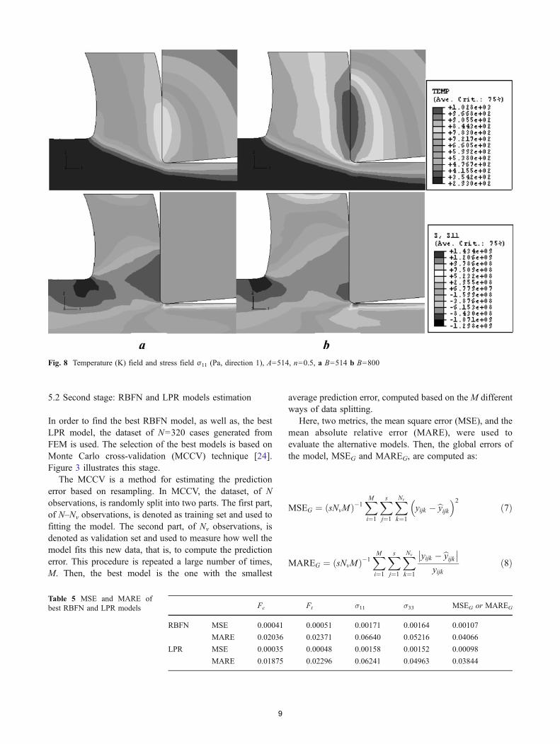
Residual stresses results from the interaction of differentcoupled phenomena. Temperature increase implies boththermal softening and enhanced thermal expansion contri-bution, having opposite effects in resultant residual stress[11]. During cutting simulation, significant influence ofinput parameters in chip morphology and stress andtemperature fields was observed. Some examples of thetemperature and σ11 fields during cutting are shown inFigs. 7 and 8. In the simulations presented in Fig. 7, thesame value of parameters A=514 and B=800 MPa wereconsidered, while n was equal to 0.4, 0.5 and 0.6. Figure 8shows the influence of B, being equal to 514 and 800 MPa,respectively, while the other parameters were A=514 MPaand n=0.5. The increment of A, being the elastic limit, ledto decreased values of tensile residual stresses. The incrementof B and n, representing increased hardening originated largervalues of residual stresses. These trends observed in this workare in agreement with those presented in [20].

Fig. 7 Temperature (K) and stress field σ11 (Pa, direction 1) obtained for A=514 B=800 a n=0.4 b n=0.5, c n=0.6

Table 4 Intervals of input parameters for numerical simulations andcorresponding intervals of output parameters used for training nonparametric models

Input parameters Output parameters

A (MPa) 300–600 Fc (N/mm) 156–470

B (MPa) 500–900 Ft (N/mm) 76–386

n 0.3–0.6 σ11 (MPa) 162–1,540

μ 0.3–0.8 σ33 (MPa) 272–1,420

8

5.2 Second stage: RBFN and LPR models estimation

In order to find the best RBFN model, as well as, the bestLPR model, the dataset of N=320 cases generated fromFEM is used. The selection of the best models is based onMonte Carlo cross-validation (MCCV) technique [24].Figure 3 illustrates this stage.

The MCCV is a method for estimating the predictionerror based on resampling. In MCCV, the dataset, of Nobservations, is randomly split into two parts. The first part,of N–Nv observations, is denoted as training set and used tofitting the model. The second part, of Nv observations, isdenoted as validation set and used to measure how well themodel fits this new data, that is, to compute the predictionerror. This procedure is repeated a large number of times,M. Then, the best model is the one with the smallest

average prediction error, computed based on the M differentways of data splitting.

Here, two metrics, the mean square error (MSE), and themean absolute relative error (MARE), were used toevaluate the alternative models. Then, the global errors ofthe model, MSEG and MAREG, are computed as:

MSEG ¼ sNvMð Þ�1XMi¼1

Xs

j¼1

XNv

k¼1

yijk �byijk� �2ð7Þ

MAREG ¼ sNvMð Þ�1XMi¼1

Xs

j¼1

XNv

k¼1

yijk � byijk yijk

ð8Þ

Fig. 8 Temperature (K) field and stress field σ11 (Pa, direction 1), A=514, n=0.5, a B=514 b B=800

Fc Ft σ11 σ33 MSEG or MAREG

RBFN MSE 0.00041 0.00051 0.00171 0.00164 0.00107

MARE 0.02036 0.02371 0.06640 0.05216 0.04066

LPR MSE 0.00035 0.00048 0.00158 0.00152 0.00098

MARE 0.01875 0.02296 0.06241 0.04963 0.03844

Table 5 MSE and MARE ofbest RBFN and LPR models

9

where, s is the number of output variables, y is the realvalue, and by the estimated value.

The results showed in this section are based on avalidation set of Nv=25 observations, and a value of M=5,000 iterations. The number of output variables is s=4.Because variables span over different ranges, all variablesare normalized between 0 and 1. Since the selection ofkernel functions is not critical to the performance of thenonparametric fit [7], the kernel in all models (RBFN orLPR) is the Gaussian function.

Therefore, for RBFN models, the parameters thatshould be determined were Tj, Cj, wjk, in Eqs. (2) and(3), and the number of hidden neurons, J. For LPR models,the parameters were the bandwidths hj, in Eq. (6), and thepolynomial degree d.

In the case of LPR models, since variables have beennormalized between [0,1], all bandwidths are set the same,that is, hj=h, j=1,2,3,4.

For RBFN models, the orthogonal least square (OLS) isused as learning procedure [25]. The OLS uses the samevalue Tj (that is, Tj=T) for all hidden neurons. For a givenT, the algorithm optimized the number of hidden neurons, J,their centres Cj, and the output layer weights, wjk. Hence, in

order to select the best RBFN model, only the parameterh is controlled.

The Matlab is used for this analysis. The parameters ofthe best estimated models were the following:

& RBFN: T=2.27 and J=120 hidden neurons. Thelocation of the centres Cj, and the output weights, wjk,are not listed for simplicity.

& LPR: h=0.13 and d=3.

Table 2 shows the MSE and the MARE for thesemodels. We can conclude that both models have similarperformance with LPR showing a better overall perfor-mance. Both metrics have very low values, showing theefficiency of the models. The MARE for variables Fc,and Ft, has a value around 2%. In the case of variablesσ11and σ33,this error has a value around 6% and 5%,respectively.

5.3 Third stage: prediction of constitutive parameters A, Band n

In this stage, a set of Fc, Ft, σ11, and σ33, as well as, theparameter μ (obtained as the ratio between thrust and

Table 6 APE (%) of the constitutive parameters using RBFN model

A bA APE (%) B bB APE (%) n bn APE (%)

363 302.27 16.73 742 775.81 4.56 0.46 0.40 12.78

385 387.68 0.70 533 500.00 6.19 0.38 0.46 20.82

457 491.95 7.65 624 764.34 22.49 0.44 0.39 10.25

464 549.13 18.35 818 847.45 3.60 0.57 0.51 9.84

471 366.81 22.12 752 851.26 13.20 0.41 0.35 14.17

532 509.24 4.28 596 672.92 12.91 0.52 0.51 2.38

565 563.23 0.31 810 852.39 5.23 0.33 0.31 5.48

567 587.25 3.57 876 899.90 2.73 0.34 0.32 6.18

592 542.53 8.36 846 713.84 15.62 0.54 0.59 8.94

641 614.07 4.20 641 889.94 38.84 0.55 0.44 19.24

Table 7 APE (%) of the constitutive parameters using LPR model

A bA APE (%) B bB APE (%) n bn APE (%)

363 430.20 18.51 742 725.42 2.23 0.46 0.48 4.74

385 355.93 7.55 533 500.10 6.17 0.38 0.45 18.34

457 524.92 14.86 624 627.31 0.53 0.44 0.45 1.84

464 402.08 13.34 818 807.46 1.29 0.57 0.56 2.30

471 379.84 19.35 752 857.07 13.97 0.41 0.35 15.15

532 552.97 3.94 596 556.21 6.68 0.52 0.57 9.96

565 584.21 3.40 810 822.65 1.56 0.33 0.32 2.39

567 547.99 3.35 876 798.91 8.80 0.34 0.34 1.41

592 526.60 11.05 846 899.76 6.35 0.54 0.51 4.98

641 646.73 0.89 641 629.26 1.83 0.55 0.58 5.82

10

cutting force) are known (Table 5). The objective is topredict the values of parameters A, B and n. As mentionedin section 1, an optimization problem is solved. At iterationi, a set of random values A(i), B(i) and n(i) along with the

value μ are used as input variables of RBFN or LPR model.Then, the values bFcðiÞ; bFtðiÞ; bs11ðiÞ and bs33ðiÞ are estimated.These values are used to compute the error, E, as:

E ¼Fc � bFcðiÞ

Fcþ

Ft � bFtðiÞ

Ftþ s11 � bs11ðiÞ

s11

þ s33 � bs33ðiÞ

s33ð9Þ

The genetic algorithm is used to minimize the error E [26].The values A(i), B(i) and n(i) that minimize E are thepredicted parameters.

Here, we show the predicted parameters bA; _bB and bn, for aset of ten cases. These cases are obtained from the FEM andthey have not been used in stage 2. The error used to evaluatethe prediction performance is the absolute percentage error(APE):

APEð%Þ ¼ y� byj jy

� 100 ð10Þ

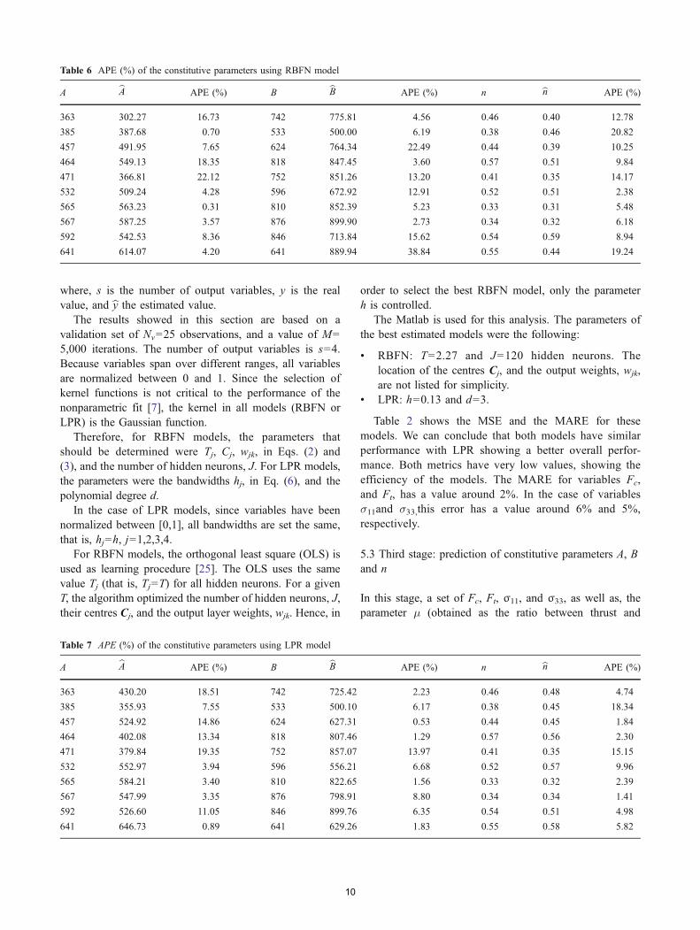
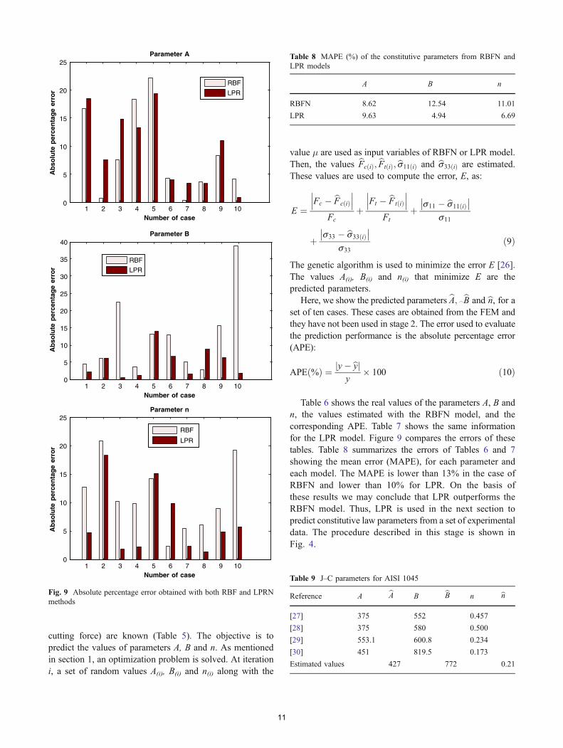
Table 6 shows the real values of the parameters A, B andn, the values estimated with the RBFN model, and thecorresponding APE. Table 7 shows the same informationfor the LPR model. Figure 9 compares the errors of thesetables. Table 8 summarizes the errors of Tables 6 and 7showing the mean error (MAPE), for each parameter andeach model. The MAPE is lower than 13% in the case ofRBFN and lower than 10% for LPR. On the basis ofthese results we may conclude that LPR outperforms theRBFN model. Thus, LPR is used in the next section topredict constitutive law parameters from a set of experimentaldata. The procedure described in this stage is shown inFig. 4.

1 2 3 4 5 6 7 8 9 100

5

10

15

20

25

Number of case

1 2 3 4 5 6 7 8 9 10Number of case

1 2 3 4 5 6 7 8 9 10Number of case

Ab

solu

te p

erce

nta

ge

erro

rParameter A

RBF

LPR

0

5

10

15

20

25

30

35

40

Ab

solu

te p

erce

nta

ge

erro

r

Parameter B

RBF

LPR

0

5

10

15

20

25

Ab

solu

te p

erce

nta

ge

erro

r

Parameter n

RBF

LPR

Fig. 9 Absolute percentage error obtained with both RBF and LPRNmethods

Table 8 MAPE (%) of the constitutive parameters from RBFN andLPR models

A B n

RBFN 8.62 12.54 11.01

LPR 9.63 4.94 6.69

Table 9 J–C parameters for AISI 1045

Reference A bA B bB n bn[27] 375 552 0.457

[28] 375 580 0.500

[29] 553.1 600.8 0.234

[30] 451 819.5 0.173

Estimated values 427 772 0.21

11

5.4 Inverse identification from experimental data

Since LPR model gives the better prediction, it is used forinverse estimation of constitutive law parameters of twotypes of steels: AISI 1045 and AISI 316L. Experimentaldata for these steels were obtained from the scientificliterature to be used as an input for the inverse identificationmethod.

Experimental data for stainless steel AISI 1045, obtainedfrom comparable cutting conditions were obtained fromreference [27]. The data from [27] were Fc=652N/mm, Ft=338N/mm and σ11=530MPa. The value of σ33 wasconsidered to be approximately the same as σ11, becauseno data was found about this parameter. Table 9 shows theestimated values for A, B and n obtained by using theproposed inverse identification methodology and thosevalues of Fc, Ft, σ11 and σ33 and also summarizes thevalues of these parameters for the AISI 1045, found inthe literature [28–31]. As shown in Table 9, the resultsprovided by the proposed inverse methodology lied inthe range of the available material parameters. Theresults were especially very close to those proposed byÖzel [31].

The methodology is also applied to the data given in thework of Outeiro et al. [32] concerning the machininginduced residual stresses in AISI 316L. The values used areFc=291 N/mm, Ft=237 N/mm, σ11=900 MPa and σ33=600 MPa. In this case, the material constants obtained withthe proposed method are shown in Table 10. These valuesare in the range proposed in the works [33–35] andsummarized in Table 10.

In order to check the material parameters by inverseidentification, the values given for both materials (AISI1045 and AISI 316L) by the LPR model were implementedin the numerical model. Numerical output (forces andresidual stresses) were compared with those presented inthe references [26–32]. The error values for cutting forcesobtained from numerical simulation were similar to thoseobtained in the experimental validation of the numericalmodel presented previously. The same trend was observedfor residual stresses. The level of tensile residual stresses in

the machined surface was underestimated with an errorclose to 20%; however as was explained before, thisphenomenon could be related with the effect of previouspasses inducing subsurface hardening in the workpiece.These results are reasonably, having into account that theerrors are due not only to the estimation method. Alsothe inexactitude derived from the use of experimentalvalues obtained from literature (due for instance topossible different treatments or processing routes of theworkpiece material, or to uncertainties of the measure-ment in each experiment) influences the errors of thefinal result.

6 Conclusions

The main contribution of this paper is the exploration of thepotentiality of the methodology developed, that has provedits ability to perform inverse identification of materialparameters from cutting tests. RBFN and LPR models wereused to identify these parameters from experimental dataobtained from cutting tests. These models are useful toolsin prediction of variables with complex dependence oninput data. Finite element analysis was performed to trainthe nonparametric models. Different methodology stageswere covered successfully. Firstly the numerical model wasdeveloped and validated showing reasonably accuracywhen compared with experimental data. Secondly, thenonparametric models were trained with FE output andwere able to predict material parameters with acceptableerrors. Finally, the method was applied to experimentaldata (cutting forces and residual stresses) obtained fromliterature focused on machining of two types of stainlesssteel. Although LPR has not been commonly used inanalysis of manufacturing processes, this method presentedlower level of error. In fact the constitutive parametersobtained with the LPR model agreed reasonably with therange of values presented in literature for each materialanalyzed.

The proposed methodology could be easily extended topredict also strain rate hardening and thermal softeningterms of the constitutive equation. Future work in thetopic presented in the paper would also involve improvedtesting procedure with the measurement of other signif-icant variables during cutting (mainly temperature).Furthermore, other representative parameters obtainedfrom numerical simulation could be used, for instancethe geometrical characteristics of the chip morphology,strongly dependent on constitutive law parameters. Alsothe numerical modelling could be improved considering3D codes and more sophisticated contact laws or otheradvanced constitutive equations. The improvement ofeach stage involved in the presented methodology would

Table 10 J–C parameters for AISI 316L

Reference A bA B bB n bn[32] 305 1,161 0.61

[32] 305 441 0.10

[33] 301 1,472 0.807

[34] 280 1,750 0.8

[3] 514 514 0.508

Estimated values 330 822 0.4

12

lead to improvements in the final inverse identificationprocedure.

Acknowledgments The authors acknowledge the financial supportof this work to the Ministry of Science and Education of Spain(under project DPI2008-06746).

References

1. Gonzalo O, Jauregi H, Uriarte L, López de Lacalle L (2009)Prediction of specific force coefficients from a FEM cuttingmodel. Int J Adv Manuf Technol 43:348–356

2. Davim J, Maranhão C, Jackson M, Cabral G, Grácio J (2009) FEManalysis in high speed machining of aluminium alloy (Al7075-0)using polycrystalline diamond (PCD) and cemented carbide (K10)cutting tools. Int J Adv Manuf Technol 39:1093–1100

3. Tounsi N, Vincenti J, Otho A, Elbestawi MA (2002) From thebasics of orthogonal metal cutting toward the identification of theconstitutive equation. Int J Mach Tools Manuf 42/2:1373–1383

4. Kuo C-FJ, Wu Y-S (2005) Application of a Taguchi-based neuralnetwork prediction design of the film coating process for polymerblends. Int J Adv Manuf Technol 27:455–461. doi:10.1007/s00170-004-2215-3

5. Kohli A, Dixit US (2005) A neural-network-based methodologyfor the prediction of surface roughness in a turning process. Int JAdv Manuf Technol 25(1/2):118–129

6. Sanjay C, Jyothi C (2006) A study of surface roughness in drillingusing mathematical analysis and neural networks. Int J AdvManuf Technol 29:846–852

7. Härdle W (1990) Applied nonparametric regression. CambridgeUniversity Press, Cambridge, UK

8. Umbrello D, Ambrogio G, Filice L, Shivpuri R (2008) A hybridfinite element method–artificial neural network approach forpredicting residual stresses and the optimal cutting conditionsduring hard turning of AISI 52100 bearing steel. Mater Design29:873–883

9. Chamekh A, Bel Hadj Salah H, Hambli R (2009) Inversetechnique identification of material parameters using finiteelement and neural network computation. Int J Adv ManufTechnol 44:173–179. doi:10.1007/s00170-008-1809-6

10. Fernández-Fdz D, Zaera R (2008) A new tool based on artificialneural networks for the design of lightweight ceramic–metalarmour against high-velocity impact of solids. Int J Solid Struct45:6369–6383

11. Miguélez MH, Zaera R, Molinari A, Cheriguene R, Rusinek A(2009) Residual stresses in orthogonal cutting of metals: the effectof thermomechanical coupling parameters and of friction. J ThermStresses 32(3):269–289

12. Johnson GR, Cook WH (1983) A constitutive model and data formetals subjected to large strains, high strain rate and temperature.In: Proc 7th Int Symp on Ballistics. pp. 541–547.

13. Muñoz-Sánchez A, Miguélez H, Canteli JA, Cantero JL (2009)The influence of tool wear in surface integrity when machiningaustenitic stainless steel. In: 9th International Conference on theMechanical and Physical Behaviour of Materials under DynamicLoading (DYMAT 2009), Brussels, Belgium

14. Umbrello D, M’Saoubi R, Outeiro JC (2007) The influence ofJohnson–Cook material constants on finite element simulation ofmachining of AISI 316L steel. Int J Mach Tools Manuf 47:462–470

15. Hibbit Karlson and Sorensen Inc (2003) ABAQUS User’s Manual6.4–1

16. Adetoro OB, Wen PH (2010) Prediction of mechanistic cuttingforce coefficients using ALE formulation. Int J Adv ManufTechnol 46(1/4):79–90

17. Miguélez H, Muñoz-Sánchez A, Cantero JL, Loya JA (2009) Anefficient implementation of boundary conditions in an ALE modelfor orthogonal cutting. J Theor Appl Mech 47(3):1–20

18. Miguélez MH, Zaera R, Molinari A, Muñoz-Sánchez A (2009)The influence of cutting speed in the residual stresses induced byHSM in AISI 316L steel, 12th CIRP Conference on Modelling ofMachining Operations. San Sebastián, Spain.

19. Moufki A, Molinari A, Dudzinski D (1998) Modelling oforthogonal cutting with a temperature dependent friction law. JMech Phys Solids 46/10:2103–38

20. Nasr MNA, Ng EG, Elbestawi MA (2008) A modified time-efficient FE approach for predicting machining-induced residualstresses. Finite Elem Anal Des 44:149–161

21. Jang DY, Watkins TR, Kozaczek KJ, Hubbard CR, Cavin OB(1996) Surface residual stresses in machined austenitic stainlesssteel. Wear 194:168–173

22. Korkut I, Kasap M, Ciftci I, Seke U (2004) Determination ofoptimum cutting parameters during machining of AISI 304austenitic stainless steel. Mater Design 25:303–305

23. Haykin S (2007) Neural networks: a comprehensive foundation.Prentice Hall, Englewood Cliffs, NJ

24. Shao J (2003) Linear Model Selection by Cross-Validation. JAmer Stat Assoc 88:486–494

25. Chen S, Cowan CFN, Grant PM (1991) Orthogonal least squareslearning algorithm for radial basis function networks. IIEE TransNeur Netw 2:302–309

26. Goldberg DE (1989) Genetic Algorithms in Search, Optimizationand Machine Learning. Kluwer Academic Publishers, Boston,MA

27. Zouhar J, Piska M (2008) Modelling the orthogonal machiningprocess using cutting tools with different geometry. MM Sci J 48–51

28. Borkovec J, Petruska J (2007) Computer simulation of materialseparation process. In: Proc. Engineering Mechanics, Svratka,Czech Republic. p. 14.

29. Forejt M (2004) The mechanical properties of selected types ofsteel in the condition of higher speed deformation. Report ofResearch plan MSM 262100003, Brno University of Technology,Institute of Manufacturing Technology, Czech Republic

30. Jaspers SPFC, Dautzenberg JH (2002) Material behaviour inconditions similar to metal cutting: flow stress in the primaryshear zone. J Mater Process Technol 122:322–330

31. Özel T, Zeren E (2005) Finite element modeling of stressesinduced by high speed machining with round edge cutting tools.ASME InternationalMechanical Engineering Congress & Exposition,Orlando

32. Outeiro JC, Umbrello D, M’Saoubi R (2006) Experimental andnumerical modelling of the residual stresses induced in orthogonalcutting of AISI 316L steel. Int J Mach Tool Manufact 46(14):1786–1794

33. Chandrasekaran H, M’Saoubi R, Chazal H (2005) Modelling ofmaterial flow stress in chip formation process from orthogonalmilling and split Hopkinson bar tests. Mach Sci Technol 9:131–145

34. M’Saoubi R (1998) Aspects Thermiques et Microstructuraux de lacoupe. Application a la coupe orthogonale des aciers austenitiques.Ph.D. Thesis, ENSAM-Paris

35. Changeux B, Touratier M, Lebrun JL, Thomas T, Clisson J(2001) High-speed shear tests for the identification of theJohnson–Cook law. Fourth International ESAFORM Conference.pp. 603–606

13