A Global Optimization Approach for Architectural Synthesis

1266 IEEE TRANSACTIONS ON COMPUTER-AIDED DESIGN OF INTEGRATED CIRCUITS AND SYSTEMS, VOL. 12, NO. 9, SEPTEMBER 1993

Global Optimization Approach for Architectural Synthesis

Catherine H . Gebotys, Member, IEEE, and Mohamed I . Elmasry, Fellow, IEEE

Abstract-A relaxed LP model, which simultaneously schedules and allocates functional units and registers, is presented for synthesizing cost-constrained globally optimal architectures. This research is important for industry by providing exploration of optimal synthesized architectures since it is well known that early architectural decisions have the greatest impact on the final design. A mathematical integer programming formulation of the architectural synthesis problem was transformed into the node packing problem. Polyhedral theory was used to formulate constraints that decreased the size of the search space, thus improving integer programming solution efficiency. Execution times are an order-of-magnitude faster than previous research that uses heuristic techniques. This research breaks new ground by 1) simultaneously scheduling and allocating in practical execution times, 2) guaranteeing globally optimal solutions for a specific objective function, and 3) providing a polynomial run-time algorithm for solving some instances of this NP-complete problem.

I. INTRODUCTION RCHITECTURAL synthesis is an important part of A the VLSI design cycle. The objective of synthesizers

is to transform an input algorithm (or behavior) into a hardware architecture that minimizes a cost function and satisfies a set of constraints. Synthesizers must produce globally optimal architectures and execute quickly to provide early exploration of design tradeoffs. In addition, synthesizers should be able to optimize linear or piecewise linear cost functions, and incorporate complex timing constraints. The architectural synthesis problem in- volves several interdependent subtasks including scheduling, and the allocation of functional units, registers, and interconnects. The preceding problem is be- lieved to be NP-hard, since many of its subtasks have been defined as NP-complete [ 11.

Since the subtasks of architectural synthesis are highly interdependent, we must solve simultaneously for more than one subtask. The classic problem given subsequently, known as precedence constrained scheduling, is taken from 12, p. 811 and is an important subtask of the architectural synthesis problem.

Manuscript received February 21, 1991; revised December 14, 1992. This paper was recommended by Associate Editor A. Parker. The work of the first author was supported by NSERC and the University of Waterloo Start Up Grant. The work of the second author was supported in part by grants from BNR, GE, and NSERC.

The authors are with the Department of Electrical and Computer Engi- neering, University of Waterloo, Ontario, Canada.

IEEE Log Number 9207800.

“A set T ‘tasks’ (each assumed to have ‘length’ one), a partial order < * on T, a number m of ‘processors’ and an overall ‘deadline’ D E Z.

Is there a ‘schedule’ a: T .+ (0 , 1, - - , D} such that, for each i E (0, 1, - * , D}, I{t E T : a(t) = i}I +

m, and such that, whenever t < * t’, then a(t) < 0 (t)’ )?”

This problem, known as precedence constrained scheduling, is NP-complete [2] (except for two processors 131, or if the partially ordered set has an intree structure 121). In architectural synthesis, this problem (with many exten- sions that will be defined later in this paper) is called simultaneous scheduling and jimctional unit allocation. The processors are functional units and the tasks are the code operations of the input algorithm. Any input algorithm or directed acyclic graph (DAG) can be represented by a partially ordered set of code operations. The following architectural synthesis problems, 1 and 2, will be examined and solved herein.

Produce a schedule, by mapping each code operation of an input algorithm to a time and map each code operation to a functional unit. The objective is to minimize a cost function of the functional units, given an upper bound on the time to execute the input algorithm (on the synthesized architecture). Produce a schedule, as in Problem 1 and map each code operation to a functional unit and a register (which holds the variable output by the code operation, until the last code operation that uses the variable has been executed). The objective is to minimize a cost function of the functional units and registers, given an upper bound on the time to execute the input algorithm (on the synthesized architecture).

both Problems 1 and 2, the following constructs are to be supported: a) selection of single-cycle, multicycle, or pipelined functional units, b) functional pipelining (or pipelining of the input algorithm), c) conditional code, d) loops, and e) fixed, minimum, or maximum timing constraints.

Many heuristic approaches to Problem 1 have been researched in [4] and [5]. More recently, [4] has extended the stepwise refinement algorithm, HAL, to include changes in scheduling due to register and interconnect es-

0278-0070/93$03.00 0 1993 lEEE

GEBOTYS AND ELMASRY 1 ARCHITECTURAL SYNTHESIS 1267

timated effects. Problem 2 represents simultaneous scheduling, and allocation of functional units and registers. Several research projects that simultaneously optimize Problem 2 in a formal or mathematical manner are discussed subsequently.

A Mixed Integer Linear Programming (MILP) model in [6] solves Problem 2 and, in addition, simultaneously schedules in real time and selects registers and functional units from a library. Unfortunately, only very small examples could be solved due to the size of the model and the inefficiencies of the branch-and-bound technique.

A simulated annealing technique presented in [ 13 solves Problem 2 . The cost functions include a calculated number of registers and an estimated number of interconnects. Running times were achieved comparable to heuristic techniques, although the rate of convergence to a global optimum is exponential [7].

An integer programming (IP) formulation for solving Problem 1 is used to produce a schedule [8] that can minimize the number of functional units in one step and the sum of the variable lifetimes of the algorithm (or execution time) in the second step. By using a two-step meth- odology, they have shown that individual IP’s can be solved very quickly by incrementally moving across the design space and using previous allocations as an upper bound on solving for the increased number of control steps. A heuristic partitioning procedure was presented to overcome the IP limitation to small problems ( 5 200 variables [9]).

A graph-theoretical approach to the simultaneous scheduling and resource (modules and registers) minimi- zation problem was presented in [ 101. A two-dimensional placement of the data flow graph, where makespan (or execution time), graph height (number of modules), and modified cutwidth measurement (estimated number of registers) were defined, was used to represent the scheduling problem. A heuristic algorithm was used to solve the problem since the complexity was NP-complete.

General IP solving techniques, such as branch and bound [7], are very inefficient and only practical for 100- 200 variables [9]. Even general 0- 1 IP problems with linear constraints and objective functions are among the NP- complete problems for which no technically good algorithms are known to date [ l l ] . However, under certain conditions, polyhedral theory can be used to solve the IP more efficiency. Research in this area is motivated by the fact that integer programming is NP-hard, and very erratic performance is solving IP’s has been experienced. It has been proven that, for every bounded linear system of inequalities (or polytope), there exists another linear system of inequalities (integral polytope) that can be solved as a linear program (e.g., using the simplex algorithm) and always produce integer solutions [7]. Integral facets’ of the polytope are the necessary constraints required to define the integer vertices of the polytope. If these facets are

‘ A facet is a valid inequality of dimension one less than the dimension [7] of the polyhedron.

used over the region of a minimum (or maximum) objective function, then the solution of the IP can be obtained from the relaxed Linear Programming (LP) solution. Al- though for many problems it is not known what the facets look like, there are some problems, such as matching and total unimodularity [7], for which the facets have been completely characterized. In another class of problems, such as the traveling salesman problem (TSP) and the node packing problem, the facets have been partially characterized. The recent success in the TSP problem has an important impact on solving large IP’s. For example [7], the TSP with 7000 integer variables was solved in 2 min 30 s, and a 50 000-variable TSP was solved to 0.25% optimality in 30 min. Unfortunately, the large amount of research in the traveling salesman problem is not propor- tional to its applicability. Crowder et al. [ l l ] have recently shown that, even if a problem does not fall into one of these classes, yet a subset of the problem can be mapped into one of these partially characterized classes of problems, then by using facets of this subpolytope the size of the search space is reduced and large 0-1 IP problems can be solved efficiently. For example, they solved for over 2000 binary variables in under 1 h of CPU time.

The focus of this paper is on the application of node packing to architectural synthesis, which, similar to the TSP, has been partially characterized by its facets. In addition, a property unique to node packing (and not valid for any other IP) is that, if not all variables in a solution are integers, the variables that are integers remain integers in a globally optimal solution [7]. This important property will be called the decomposition property, since it can be used to decompose a large problem into a number of smaller problems.

The weighted node packing problem [7] is stated more formally as maximizing E, cuxu, where c, is a cost vector and xu is a vertex of the graph G = ( V , E ) , where

for every edge (U, U ) E E

for all nodes U E V.

xu + x,, 5 1,

xu E (0, I ) ,

The problem can also be represented as a system of linear inequalities, Ax 5 6 , where A is a (0, 1) matrix with each row having two 1’s and b is a unit vector.

Finding all integral facets for a particular node packing problem is NP-complete. This problem is known as the stable set polytope problem, using graph-theoretical terminology. Nevertheless, only integral facets over the region of the minimum (or maximum) objective function are required to obtain integer solutions. It is also important to extract some facets since they make the model very tight [7] (or reduce the size of the solution space), thus providing good bounds on the problem. The use of facets is also known to reduce the number of live nodes generated in a branch-and-bound algorithm.

We will show how our research has mapped the architectural synthesis problem into the node packing problem and by extraction and generalization of some integral facets has optimally solved Problems 1 and 2 . Synthesized


solutions of several high-level synthesis benchmarks are obtained in (CPU) execution times faster than comparable heuristic technique. The simplex algorithm [9] is currently used to schedule and allocate architectures simultaneously. The cost function can be piecewise linear, and it can handle fixed resources, cost-constrained allocation, or a combination of both. Functional units can be multi- functional (e.g., an ALU), single-cycled, multicycled or pipelined. Branches, loops, conditional code, and functional pipelining are supported. In addition, the selection of the type of functional unit (e.g., pipelined or multicycled version of a multiplier) can be optimized simultaneously.

11. PRELIMINARIES The input to the synthesizer is a list of code operations,

a table defining the partial order between code operations, the as-soon-as-possible (asap) and as-late-as-possible (alap) times for each code operation, and the cost function. The IP model, its transformation to the stable set polytope problem, and techniques used for its solution will be presented next. We will use Problem 1 to illustrate how we transformed the IP into the node packing problem and extracted integral facets, and then we will discuss the additional register allocation constraints necessary for solving Problem 2.

The following terminology is used:

k = code operation. A partial order (or precedence constraint) between k l and k2 is represented by k l < k Z , or, in other words, kl must execute before k2 [2] . Let K be the maximum number of code operations in the input algorithm. j = time or control step (cstep), J L j 2 1, j E Z (set of integers), and J = upper bound on the number of control steps. i = functional unit, i E Z. The mapping of k to i (one to many) is also defined based on the functions that each i can perform. For example, an addition code operation k, cannot be mapped to a multiplier i l , however, it may be mapped to an ALU i2 or an adder i3. Thus xl2,,,k, xL3,,,kZ are the variables generated for code operation k,. R = number of registers, R E Z . When x , , , , ~ = 1 in the IP solution, this means that code operation k is assigned to functional unit i, and the code operation starts executing at control stepj. j E R ( k ) , where R (k) = {asap (k), asap (k) + 1 ,

, alap ( k ) } , means that j is lower bounded by the asap control step and upper bounded by the alap control step for code operation k or asap (k) 5 j 5 alap (k) . k, E Op (C,, L,) means that the code operation k, has an execution time of C, (the number of control steps required by the operation to produce an output) and a latency of L, (or the minimum time between successive data inputs to the functional unit). For example, a single-cycle operation is k E Op (1, l ) , and

a two-cycle pipelined operation is k E Op(2, 1 ) . This notation is used to simplify the inequalities presented in Section 111. However, it should be noted that, in fact, each code operation can have different C and L values, depending on which functional unit it is mapped to. In Section V we will illustrate this with the notation ( k , i) E Op(C, L).

111. PROBLEM 1 : IP MODEL Problem 1, which performs simultaneous scheduling

and functional unit allocation, can be modeled as an assignment problem, where the variables are represented by x i , j ,+ . The IP model consists of three types of general constraints, as discussed below.

Equation (l), called the operation assignment constraint, ensures that each code operation will be assigned to one control step and one functional unit.

* i , j , k - - 1 , v k . i j eR(k)

Inequality (2 ) , called the functional unit constraint, prevents more than one code operation from being assigned to the same functional unit at the same control step.

ji = j - L + 1

Inequality (3), called the precedence constraint, prevents an operation k l from being scheduled after operation k2 whenever there is a partial order between these operations such that kl < * k2 .

(xi , j i ,ki + x i , j ~ , k ~ ) 5 1 , vkl < * k27 j2 I j l

x ; , ~ , ~ = O or 1. (4)

IV. TRANSFORMATION TO NODE PACKING AND FACET ANALYSIS

When we relax (4) to 0 I x I 1, the system of linear inequalities2 becomes Ax I b, where A is a (0, 1) matrix (or all entries in A are 0 or 1) and b is a unit vector. For example, consider scheduling the two operations k = a and k = b (a E Op(1, 1) b E Op(1, l)), where a must be executed before b (or a < b) , defined over csteps j = 1, 2 , 3 , 4, and 5, thus R(a) = (1, 2 , 3 , 4}, and R ( b ) = ( 2 , 3 , 4, 5 ) . For now, we assume there are two functional units i = 1, 2. The constraints for this problem generated from inequalities (1) through (3) below form the following A matfix, where x = [XI, l , a , x2,1,a, ~ 1 , 2 , a , ~ 2 , 2 , a , * * *

'Equation (1) could be transformed into an (5) inequality by using a maximization objective function, such as max Ex. However, we use (1) directly. This had no effect on the efficiency of solving the IP.

I269 GEBOTYS AND ELMASRY: ARCHITECTURAL SYNTHESIS

X 1 , 5 , b , x 2 , 5 , bl:

(3)

Row No. Inequality No.

(1)

(2)

This problem, known as set packing [any problem with A a (0, 1) matrix and a unit b vector, and binary x ] [7], can be transformed into a graph, G = ( V , E ) (called the node packing graph), from which we can extract some integral facets of the node packing problem. First, we map each variable, x ~ , ~ , ~ , into a node, u E I/. Edges of the graph, E, are defined by the following procedure. For each row of the matrix A (representing a constraint), the variables

in G [7]. The graph G represents the node packing problem, which can be transformed from any system of linear inequalities with a (0, 1) constraint matrix (A) and a unit vector (6) on the right-hand side. Known integral facets

5 1 , for all K cliques (or maximal complete subgraphs), and ii) C l r s C x U I (\Cl - 1)/2, for all C chordless odd

procedure for odd cycles. For simplicity, first we will examine the one-dimen-

sional (1-D) problem, where the variables are x , , k for all Jegk,) ( j 1x1 ki - c ( j ) X J , k2 5 - C I , V ~ I < * k2. j , k. Again consider the scheduling problem for code operations a and b, where a < e b and J = 5. Constraints We will call this constraint ( 5 * ) . Although the set of in- (1) and (3) [with i = 1 , and (2) is no longer valid for the teger feasible solutions is the same, formulation (5) is 1-D model] are used to generate the following F matrix, tighter (or forms a smaller search space) than ( 5 ” ) and the where Fx 5 1 and xT = [xl,., x2,., x3, . , x4, . , x 2 , b , x 3 , b , proof is given in Appendix I . Thus improvements in IP

x J , . and x J , b . In Fig. l(b) we note that the four nodes, x3, . , x4,., x Z , b , x 3 , b , shown in bold, form a clique, or integral facet ( i ) . The edges of this clique were formed by rows (1. l ) , (1.2), and (3.2)-(3.5) of matrix F. The clique can be represented by the inequality x 3 , . + ~ 4 , . + X 2 , b -k X 3 . b

5 1. Therefore, (3.2)-(3.5) can be replaced by the following row:

(or columns) with a “1”entry define a complete subgraph3 [ O O 1 1 1 1 0 0 1 .

We can generalize this clique facet (precedence a m - straint) to

c X ~ 2 9 k 2 + x J l , k l v k , < * k 2 , for the node packing problem are as follows: i) C u c K xu ~ 2 5 . 1 J I 21 -cI + 1 J I ER(ki ) J 2 E R ( k 2 )

j E R(k2) rl (R(ki) + ( C I - l)), ki E 0 p ( C 1 , L I )

straint formulation was presented in [8] and [12] as

(5 ) cycles, (cl 2 5 and others in [71 that involve a lifting A different formulation of the 1-D precedence con-

J E R (A21

X 4 , b , X5,bl:

Row No. Inequality No.

( 1 )

(3)

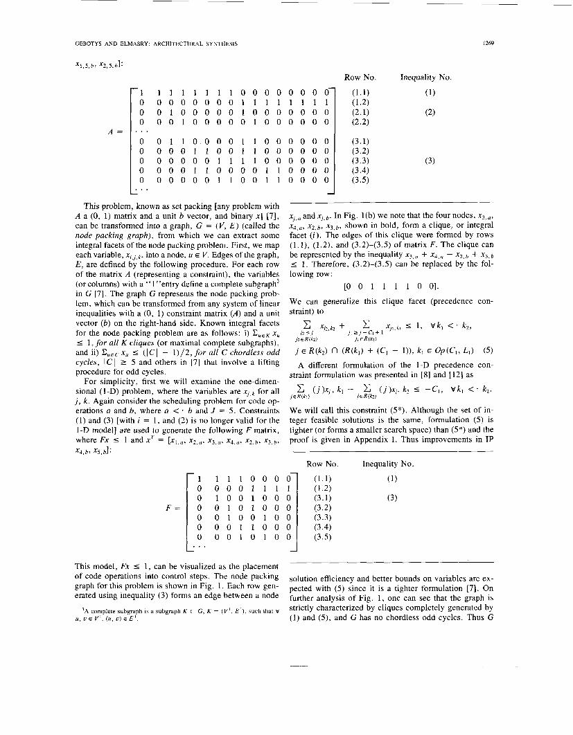
This model, Fx I I , can be visualized as the placement Of code Operations into control steps. The node packing graph for this problem is shown in Fig. 1 . Each row gen- crated using (3) forms an edge between a node

solution efficiency and better bounds on variables are expected with (5) since it is a tighter formulation [7]. o n further analysis of Fig. 1, one can see that the graph is

’A complete subgraph 1s a subgraph K c G, K = (VI, E l ) , such that v characterized by completely generated by U , v E V ’ , ( U , U ) E El (1) and ( 5 ) , and G has no chordless odd cycles. Thus G

1270 IEEE TRANSACTIONS ON COMPUTER-AIDED DESIGN OF INTEGRATED CIRCUITS AND SYSTEMS, VOL. 12, NO. 9 , SEPTEMBER 1993

(a) (b) (a) (b) Fig. 1. Node packing graph for two code operations (a < . b), showing in bold a clique facet f o r j = 2 in (a) a n d j = 3 in (b) of inequality (5). R(a)

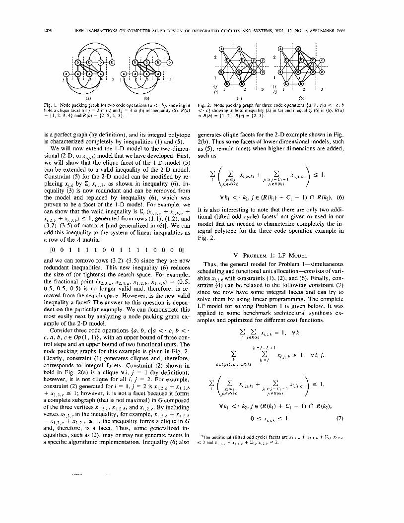
Fig. 2. Node packing graph for three code operations { a , b, cia < . c , 6 < . c } showing in bold inequality (2) in (a) and inequality ( 6 ) in (b). R ( a )

= { 1, 2 , 3 , 4) and R(b) = (2 , 3 , 4, 5). = R(b) = (1, 2} , R ( c ) = (2, 3 ) .

is a perfect graph (by definition), and its integral polytope is characterized completely by inequalities (1 ) and (5).

We will now extend the 1-D model to the two-dimensional (2-D, orxi,j,k) model that we have developed. First, we will show that the clique facet of the 1-D model (5) can be extended to a valid inequality of the 2-D model. Constraint (5) for the 2-D model can be modified by re- placing xj,k by Ci x ; , ~ , ~ , as shown in inequality (6). In- equality (3) is now redundant and can be removed from the model and replaced by inequality (6) , which was proven to be a facet of the 1-D model. For example, we can show that the valid inequality is Ci + x ; , ~ , ~ + xi, 2 , b + xi, 3 , b ) I 1 , generated from rows ( 1 . l ) , (1.2), and (3.2)-(3.5) of matrix A [and generalized in ( 6 ) ] . We can add this inequality to the system of linear inequalities as a row of the A matrix:

[O 0 1 1 1 1 0 0 1 1 1 1 0 0 0 01

and we can remove rows (3.2)-(3.5) since they are now redundant inequalities. This new inequality (6) reduces the size of (or tightens) the search space. For example,

0.5, 0.5, 0.5) is no longer valid and, therefore, is removed from the search space. However, is the new valid inequality a facet? The answer to this question is depen- dent on the particular example. We can demonstrate this most easily next by analyzing a node packing graph example of the 2-D model.

c , a, b, c E Op ( 1 , l)], with an upper bound of three control steps and an upper bound of two functional units. The node packing graphs for this example is given in Fig. 2. Clearly, constraint (1) generates cliques and, therefore, corresponds to integral facets. Constraint (2) shown in bold in Fig. 2(a) is a clique V i , j = 1 (by definition); however, it is not clique for all i, j = 2. For example, constraint (2) generated for i = 1 , j = 2 is x ~ , ~ , ~ + x , , ~ , ~ + x1,2,c I 1; however, it is not a facet because it forms a complete subgraph (that is not maximal) in G composed of the three vertices x ~ , ~ , xl, 2,b , and x ~ , ~ , =. By including vertex x 2 , 2 , c in the inequality, for example, x ~ , ~ , ~ + x ~ , ~ , ~ + x1,2 ,c + x2 ,2 ,c I 1 , the inequality forms a clique in G and, therefore, is a facet. Thus, some generalized inequalities, such as (2), may or may not generate facets in a specific algorithmic implementation. Inequality (6) also

the fractional point ( x 2 , 3 , a , X2,4,a, x 1 , 2 , b , x 1 , 3 , b ) = (0.5,

Consider three code operations {a , b, c ( a < c, b <

generates clique facets for the 2-D example shown in Fig. 2(b). Thus some facets of lower dimensional models, such as ( 5 ) , remain facets when higher dimensions are added, such as

v k ~ < - k2, j E ( R ( ~ I ) + CI - 1) n R W , (6)

It is also interesting to note that there are only two additional (lifted odd cycle) facets4 not given or used in our model that are needed to characterize completely the integral polytope for the three code operation example in Fig. 2.

V. PROBLEM 1: LP MODEL Thus, the general model for Problem 1-simultaneous

scheduling and functional unit allocation-consists of vari- a b l e s ~ ; , ~ , ~ with constraints ( l ) , (2), and (6 ) . Finally, constraint (4) can be relaxed to the following constraint (7) since we now have some integral facets and can try to solve them by using linear programming. The complete LP model for solving Problem 1 is given below. It was applied to some benchmark architectural synthesis examples and optimized for different cost functions.

X i , j , k - - 1, vk. i j E R ( k )

i i = i - L + 1 c c i 1= i

Xi, j i ,k 1 , V i , j .

vk, < k2, j E ( R ( k l ) + C1 - 1) fl R(k2) ,

0 5 x;,j,k 5 1. (7)

4The additional (lifted odd cycle) facets are x2. I , u + x2. I . h + E,,,, x , ,~ . , , 5 2 a n d x , , , , , + X i . i . h + E, k X t , 2 . k 5 2.

GEBOTYS AND ELMASRY: ARCHITECTURAL SYNTHESIS 1271

VI. PROBLEM 2: CONSTRAINT FOR

REGISTER ALLOCATION The LP model for Problem 2-simultaneous scheduling

and functional unit and register allocation-is exactly the same as the LP model presented in Section V (for solving Problem 1) except additional constraints are generated for register allocation. The register allocation constraint required for this model requires some preprocessing. We have researched many different formulations [ 131 for register allocation. The formulation that gave the best performance (in terms of CPU time to solve the optimization problem) will be presented subsequently.

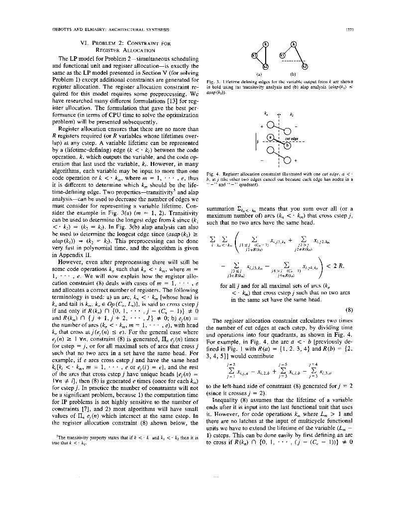
Register allocation ensures that there are no more than R registers required (or R variables whose lifetimes over- lap) at any cstep. A variable lifetime can be represented by a (lifetime-defining) edge (k < k,) between the code operation, k, which outputs the variable, and the code operation that last used the variable, kl. However, in many algorithms, each variable may be input to more than one code operation or k < k,, where rn = 1, * , e , thus it is different to determine which k, should be the lifetime-defining edge. Two properties-transitivity5 and alap analysis-can be used to decrease the number of edges we must consider for representing a variable lifetime. Con- sider the example in Fig. 3(a) (rn = 1, 2). Transitivity can be used to determine the longest edge from k since (k, < k2) =$ (k2 = k,). In Fig. 3(b) alap analysis can also be used to determine the longest edge since (asap(k2) 2 alap (k,)) =$ (k2 = k, ) . This preprocessing can be done very fast in polynomial time, and the algorithm is given in Appendix 11.

However, even after preprocessing there will still be some code operations k, such that k, < * k,, where m = 1, * - . , e . We will now explain how the register allo-

and allocates a correct number of registers. The following terminology is used: a) an arc, k, < k, [whose head is k, and tail is k,, k, E Op(C,, L,)], is said to cross cstep j if and only if R(k,) n (0, 1, * , j - (C, - I )} # 0 andR(k,) n { j + 1 , j + 2, * * , J } # 0; b) e j (n ) = the number of arcs (k, < k,, rn = 1, - - , e), with head k, that cross at j (ej (n) I e ) . For the general case where ej(n) 1 1 Vn, constraint (8) is generated, 11, ej(n) times for cstep = j , or for all maximal sets of arcs that cross j such that no two arcs in a set have the same head. For example, if e arcs cross c s t e p j and have the same head ki[ki < * , e or e j ( i ) = e ] , and the rest of the arcs that cross cstep j have unique heads [e, (n ) = 1Vn # i], then (8) is generated e times (once for each k,) for cstepj. In practice the number of constraints will not be a significant problem, because 1) the computation time for IP problems is not highly sensitive to the number of constraints [7], and 2) most algorithms will have small values of 11, e j (n ) which intersect at the same cstep. In the register allocation constraint (8) shown below, the

cation constraint (8) deals with cases of rn = 1, * , e

k,, m = 1,

'The transitivity property states that if k < . k , and k , < . k2 then it is true that k < . k, .

(a) (b) Fig. 3. Lifetime defining edges for the variable output from k are shown in bold using (a) transitivity analysis and (b) alap analysis (a lap(k , ) 5 asap ( k d .

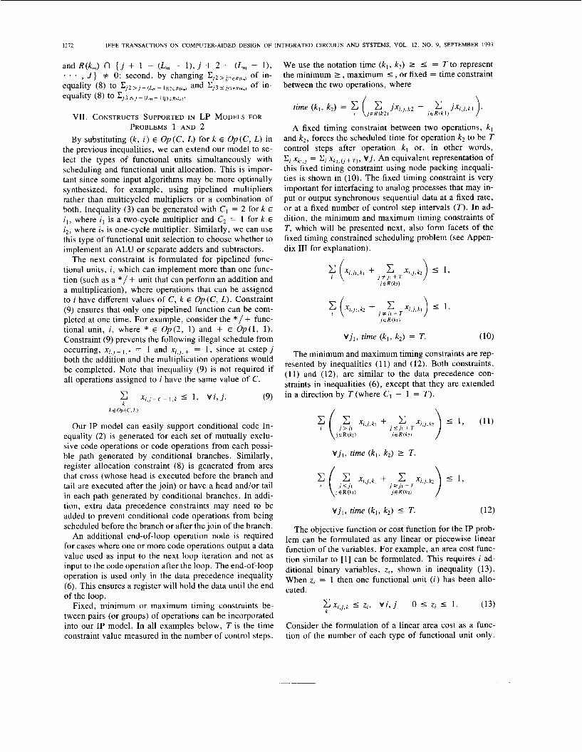
Fig. 4. Register allocation constraint illustrated with one cut edge, a < . b, at j (the other two edges cancel out because each edge has nodes in a "+" and "-" quadrant).

summation c k n < . k m means that you sum over all (or a maximum number of) arcs (k, < k,) that cross cstep j , such that no two arcs have the same head.

- j 3 5 j X i , j 3 , k , - j 4 > j - ( C n - l ) c X i , j 4 , k , ) < 2 R , j 3 E R (km) j 4 E R ( k d

for all j and for all maximal sets of arcs (k, < - k,) that cross cs tepj such that no two arcs in the same set have the same head.

(8) The register allocation constraint calculates two times

the number of cut edges at each cstep, by dividing time and operations into four quadrants, as shown in Fig. 4. For example, in Fig. 4, the arc a < b [previously defined in Fig. l with R(a) = (1, 2 , 3 , 4) and R(b) = (2 , 3, 4, 5 } ] would contribute

j = 2 j = 5 j = 4

X i , j , a - Xi,2,b + ] = 3 .x x i , j , b - j s 3 X i . 3 . a j = 1

to the left-hand side of constraint (8) generated f o r j = 2 (since it crossesj = 2).

Inequality (8) assumes that the lifetime of a variable ends after it is input into the last functional unit that uses it. However, for code operations k, where L, > 1 and there are no latches at the input of multicycle functional units we have to extend the lifetime of the variable (L, - 1) csteps. This can be done easily by first defining an arc to cross if R(k,) r l (0, 1 , , ( j - (C, - 1))) # 0 -


and R(k, ) fl { j + 1 - (L, - l ) , j + 2 - (L, - 11, . . . , J } # 0; second, by changing CJ2>J12sR(k,n, of in-

(8) to > J - (Lm - 1 ) j 2 t R ( I m ) and ‘ J 3 s J j 3 ~ R ( k , , , ) Of inequality (8) to ‘ J 3 5 J - ( L m - I ) j 7 s R ( k m ) ’

VII. CONSTRUCTS SUPPORTED I N LP MODELS FOR PROBLEMS 1 AND 2

By substituting ( k , i ) E Op(C, L) for k E Op(C, L) in the previous inequalities, we can extend our model to select the types of functional units simultaneously with scheduling and functional unit allocation. This is important since some input algorithms may be more optimally synthesized, for example, using pipelined multipliers rather than multicycled multipliers or a combination of both. Inequality (3) can be generated with C, = 2 for k E i , , where i l is a two-cycle multiplier and C2 = 1 for k E i 2 , where i2 is one-cycle multiplier. Similarly, we can use this type of functional unit selection to choose whether to implement an ALU or separate adders and subtractors.

The next constraint is formulated for pipelined functional units, i , which can implement more than one function (such as a * / + unit that can perform an addition and a multiplication), where operations that can be assigned to i have different values of C, k E Op(C, L). Constraint (9) ensures that only one pipelined function can be completed at one time. For example, consider the * / + functional unit, i , where * E Op(2, 1) and + E Op(1, 1). Constraint (9) prevents the following illegal schedule from occurring, x , , ~ - ,,* = 1 and x,,~,.+ = 1, since at cstep j both the addition and the multiplication operations would be completed. Note that inequality (9) is not required if all operations assigned to i have the same value of C.

C ~ , , ~ - c + i , k ~ 1, v i , j . (9) k

k E Op(C, L)

Our IP model can easily support conditional code In- equality (2) is generated for each set of mutually exclu- sive code operations or code operations from each possible path generated by conditional branches. Similarly, register allocation constraint (8) is generated from arcs that cross (whose head is executed before the branch and tail are executed after the join) or have a head and/or tail in each path generated by conditional branches. In addition, extra data precedence constraints may need to be added to prevent conditional code operations from being scheduled before the branch or after the join of the branch.

An additional end-of-loop operation node is required for cases where one or more code operations output a data value used as input to the next loop iteration and not as input to the code operation after the loop. The end-of-loop operation is used only in the data precedence inequality (6). This ensures a register will hold the data until the end of the loop.

Fixed, minimum or maximum timing constraints between pairs (or groups) of operations can be incorporated into our IP model. In all examples below, T is the time constraint value measured in the number of control steps.

We use the notation time ( k , , k2) I I = T to represent the minimum 2 , maximum I, or fixed = time constraint between the two operations, where

A fixed timing constraint between two operations, k l and k2, forces the scheduled time for operation k2 to be T control steps after operation kl or, in other words, Ci xk,,, = Ci x ~ , ~ + T ) , v j . An equivalent representation of this fixed timing constraint using node packing inequalities is shown in (10). The fixed timing constraint is very important for interfacing to analog processes that may input or output synchronous sequential data at a fixed rate, or at a fixed number of control step intervals ( T ) . In addition, the minimum and maximum timing constraints of T, which will be presented next, also form facets of the fixed timing constrained scheduling problem (see Appen- dix 111 for explanation).

V j , , time ( k , , k2) = T. (10)

The minimum and maximum timing constraints are represented by inequalities (1 1) and (12). Both constraints, (11) and (12), are similar to the data precedence constraints in inequalities (6 ) , except that they are extended in a direction by T (where C, - 1 = T ) .

V j , , time ( k , , k2) I T.

V j , , time ( k , , k2) I T, (12)

The objective function or cost function for the IP problem can be formulated as any linear or piecewise linear function of the variables. For example, an area cost function similar to [ l ] can be formulated. This requires i additional binary variables, z i , shown in inequality (13). When zi = 1 then one functional unit ( i ) has been allocated.

C X ~ , ~ , ~ I z i , v i , j o I zi I 1 . (13)

Consider the formulation of a linear area cost as a function of the number of each type of functional unit only.

k

GEBOTYS AND ELMASRY: ARCHITECTURAL SYNTnEsIs 1273

Assume a+ is the area of an adder, a* is the area of a multiplier, i = 1 , 2, 3 represents the multipliers, and i = 4, 5 , 6 represents the adders. Then the linear area cost can be formulated as follows:

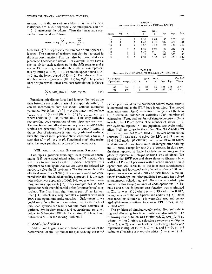
TABLE I SYNTHESIS USING LP MODEL FOR EWF (ON RC6280)

Tgen, Texe, csteps *PI * + s Var Eqn Itns S

I = 3 1 = 6

Area = a* c z, + a+ C z I . r = l 1 = 4

Note that C: E z , represents the number of multipliers allocated. The number of registers can also be included in the area cost function. This can also be formulated as a piecewise linear cost function. For example, if we have a cost of 10 for each register up to the fifth register and a cost of 15 for all registers after the sixth, we can represent this by letting R = R I + R2, where the upper bound of R I = 5 and the lower bound of R2 = 0. Then the cost function becomes cost-reg R = (10 15) (R , R2)T. The general linear or piecewise linear area cost formulation is shown as

(14)

Functional pipelining for a fixed latency (defined as the time between successive starts of an input algorithm), I , can be incorporated into our model without additional variables. We define r J / l 1 = p pipestages, and replace

where addition ( j + n l ) is modulo 1. Thus only variables representing code operations of one pipestage are used. The functional unit allocation and register allocation constraints are generated for l consecutive control steps. If the number of pipestages is less than p (defined earlier), then the model must generate these constraints for all j such that ( J - p l ) 1 j 1 p l . Functional pipelining main- tains the node packing structure of the inequalities.

C z, cost-@(i) + cost-reg R. I

C k , E ~ ( ~ ) XI,,,^ of (2) and (8) with C k ( , + n i ) E ~ ( ~ ) X r , , + n l , k

VIII. ARCHITECTURAL SYNTHESIZER RESULTS Two input algorithms from high-level synthesis bench-

marks [14] were synthesized using the LP model. (We will refer to our model as the LP model; however, it is important to note again that we are using the relaxed LP model to solve the IP problem.) The first example is the elliptical wave filter (EWF). It was synthesized and compared with the simulated annealing approach [ 11, the stepwise refinement approach of HAL [4], and another integer programming approach [15]. This example has 34 code operations with over 56 partial order (or precedence) constraints. The final input algorithm is part of the Kalman filter [14], which is a very complex algorithm with over 1000 code operations (fully unrolled). Unfortunately, we could only do a limited comparison due to the lack of published synthesizer results for this more complex algorithm. Synthesizer results and comparisons are given below in Subsection VIII-A for solving Problem 1 and Subsection VIII-B for solving Problem 2.

A . Results for Problem 1 Tables I and I1 give a more detailed examination of the

performance of the LP model for synthesizing the EWF

17 2 3 0.32 0.08 193 226 50 18 1 3 0 .42 0.11 292 273 124 19 1 2 1.67 1.58 391 327 221

17 3 3 0.36 0 .05 193 232 52 18 2 2 0.39 0.1 292 279 190 19 2 2 1.22 1.0 391 333 185 21 1 2 0.91 5.37 589 428 889

TABLE I1 SYNTHESIS USING LP MODEL FOR UNROLLED EWF (ON 386PC)

Tgen, Texe, Unrolled No. of Code Operations csteps *pl + s s Var Eqn Times

68 34 1 3 32 25 566 333 2 X

102 50 1 3 51 39 859 506 3 X

as the upper bound on the number of control steps (csteps) is increased and as the EWF loop is unrolled. The model generation time (Tgen), execution time (Texec) (both in CPU seconds), number of variables (Var), number of constraints (Eqn), and number of simplex iterations (Ztns) to solve the LP are given. The number of adders (+), two-cycle multipliers (*), and pipelined two-cycle multipliers (*pl) are given in the tables. The GAMS/MINOS (LP solver) and GAMS/ZOOM (IP solver) optimization software [9] was used to solve the LP’s and IP’s on an IBM PS/2 model 80 (386PC) and on an RC6280 MIPS workstation. All solutions were all-integer after solving the LP once, except for row 3 (19 csteps). In this case, the times reported in Table I include enumerating until a globally optimal all-integer solution was obtained. We unrolled the EWF two and three times to illustrate how well the LP model performs with a large number of code operations; see Table 11. In the later case simultaneous scheduling and functional unit allocation of over 100 code operations was executed in 90 s of CPU time. To the authors’ knowledge, no other published research has solved simultaneous scheduling and allocation to global opti- mums for this (large) number of code operations. In Ta- bles I and I1 the following cost function was minimized a, zi + a+ CiI; where a, = 0.49 and a+ = 0.012, using the area of the multipliers and adders in [ 161. Other cost functions similar to (14) were also used and generated all-integer solutions in similar CPU times, as described next.

The problem of simultaneously scheduling and selecting and allocating functional units was also solved. The following cost function was minimized, Ci cost-@ (i) zi, where i = 1 or 2 refers to selecting a two-cycle multiplier (C = 2, L = 2), i = 3 or 4 refers to selecting a two-cycle pipelined multiplier (C = 2, L = l ) , and i = 5 , 6, or 7 refers to allocating a one-cycle adder (C = L = 1) . An


upper bound of 18 csteps was used, and the IP problem was solved by GAMSIMINOS [9] on an MIPS RC6280 workstation. For example, cost-f i( i) = 14, 16, 31, 34, 2, 2, 2, for i = 1, 2, 3 , 4 , 5 , 6, 7 , respectively, represents a cost function where the first two-cycle multiplier has an area (or cost) of 14 units and the second two-cycle multiplier has an area of 16 units (slightly higher to account for additional interconnect area). This cost function was minimized, and after solving the LP once (requiring 0.47 s of CPU time), an all-integer solution was obtained. Two two-cycle multipliers and two adders were selected and allocated. When cost-fu(i) = 15, 16, 24, 34, 2, 2 , 2 for i = 1, 2, 3 , 4 , 5 , 6, 7 respectively, after solving the initial LP once (requiring 0.4 s of CPU time), an all-integer solution was obtained. One pipelined multiplier and three adders were selected and allocated. In both cases, the LP model had 3 12 variables and 214 inequalities.

Finally to illustrate the use of inequality (9) of Section VII, we simultaneously scheduled, allocated, and selected types of functional units, including functional units that were pipelined and could perform more than one function. The area of the architecture for the EWF example was minimized with a fixed execution time of 19 csteps. The functional units corresponding to i values were adders i = 1, 2, (Op(1, l ) ) , two-cycle pipelined multipliers i = 3 (Op(2, l)), and i = 4, 5 , 6 functional unit which can perform a one-cycle addition (Op(1, 1)) or a two-cycle pipelined multiplier (Op(2, 1)). The area of each adder was 0.012, the area of the pipelined multiplier was 0.49, and the area of each multipliedadder was 0.4. The IP problem required 748 variables, 527 equations, and 60.6 s of CPU time on RC6280 to find an architecture with an optimum area of 0.424. The solution allocated one multipliedadder functional unit and two adders.

Table I11 illustrates the importance of IP model formulation and the use of facets to generate a smaller search space. The problem is to schedule and allocate functional units simultaneously for the elliptic wave filter example with J = 19. Our solution is compared with the model presented in [12] and [15]. Both models were run on the same 386PC using the GAMS/ZOOM solver. Our model was solved for all-integer values after the initial LP. The other model [ 151 had to resort to a branch-and-bound rou- tine before an integer solution was found. Our LP model produced a globally optimal architecture 8.7 times faster (on the same 386PC with the same solver) than Hwang et al.’s model although our LP model has more constraints and more variables than their model. Again this further illustrates why solving IP problems is not highly depen- dent on the number of constraints. In both cases, the upper bounds on execution time and number of functional units were the same.

The Kalman filter example [14] consists of a large nested loop followed by a matrix multiplication. It is an important example for synthesis since it is very different from the EWF in that it contains a great deal of regularity and has large loops. Herein will present only results on optimally synthesizing an architecture for the matrix mul-

TABLE 111 LP VERSUS HWANG’S [15] MODEL (BOTH SOLVED WITH GAMS ON 386PC)

Tcpu, S Var Eqn Model csteps *pl +

Hwang 19 1 2 6001. 130 120 LP 19 1 2 69 355 201

+Could not be solved with initial LP, resorted to branch and bound.

tiplication. More details on the full Kalman filter example can be found in [13]. The matrix multiplication AV = U [where A is a 4 X 16 (row by column) matrix and v is a 16 x 1 vector] has to compute

e = 16

U, = C a,,,v,, for r = 1, 2, 3, 4 , c = 1

or in algorithmic form

for r = l to 4 { temp0 = 0; for c = l to 16 {

temp = a(r,c)*v(c) + tempo; temp0 = temp; ]

u(r) = tempo;}.

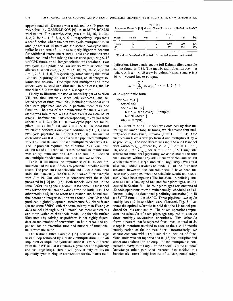
The input to our LP model was obtained by first un- rolling the inner c loop 16 times, which created four multiply-accumulate (mac) streams ( r = 1, 9 . , 4). One mac stream takes a row ( r ) from A and multiplies it by v to produce U,. The mac stream was input to our LP model with variables x ~ , ~ , ~ , where k,,,, < k + , , form = 1, , 16, and k+,,, < * k + , + , , form = 1, - * * , 15. Using constructs for functional pipelining we could model the four mac streams without any additional variables and obtain a schedule with a large amount of regularity (We could also have added variables to model all of the four mac streams; however, the controller would have been un- necessarily complex since the schedule would not necessarily have been regular.) The functional pipelining constructs used a latency of one and four pipestages, as discussed in Section V. The four pipestages (or streams) of 32 code operations were simultaneously scheduled and allocated (using the functional pipelining constraints) in 40 s of CPU time on the 386PC. Three pipelined two-cycle multipliers and three adders were allocated. Fig. 5 illustrates the optimal schedule in bold that the LP model produced for this architecture. The boxed operations represent the schedule of each pipestage required to execute three multiply-accumulate operations. This schedule forms a pattern that is repeated four times. A total of 24 csteps is therefore required to execute the 4 x 16 matrix multiplication of the Kalman filter. Unfortunately, we cannot compare with [17] since the allocation of functional units was not reported and in [ 181 the multiplier and adder are chained (or the output of the multiplier is con- nected directly to the input of the adder). To the authors’ knowledge other published research has tackled this benchmark-most likely because of its size, complexity,

1275 GEBOTYS AND ELMASRY: ARCHITECTURAL SYNTHESIS

m

4

Fig. 5 . Part of the LP optimized schedule (shown with four pipestages, latency = 1) for the 4 X 16 matrix multiplication of the Kalman filter benchmark example. The final schedule is shown in bold. The boxed schedule is repeated four times to complete the execution of the 4 X 16 matrix multiplication.

and the possible difficulties with applying heuristic synthesis techniques to an example with a great deal of regularity. Nevertheless, the matrix multiplication of the Kalman filter example illustrates the flexibility of the LP model to support functional pipelining and synthesize different types of input algorithms.

Results for Problem 2 In Table IV the synthesizers were compared by the

types of subtasks they perform and the execution time to solve the problem in CPU minutes or seconds for the EWF examples. Table IV has columns for scheduling (Sched), functional unit allocation (FU), and register allocation (Reg). A y (yes) means that the subtask is completely performed. A c (calculated) means that the number of resources is calculated exactly. An e (estimated) means that the resource is estimated using some heuristic or it is somehow considered during the algorithm. The execution time in CPU minutes/seconds in Table IV are only for the scheduling phase for HAL [4] (using a Xerox 1108 Lisp machine) and the simulated annealing (S.A.) run times (using a Vax 1118650) for [ 11. The LP model CPU seconds (Tgen + Texec) are for the GAMSIMINOS solver [9] runs on a 386PC. The asap1alap or other preprocessing times were not included but are negligible (less than 1 min of CPU time). All integer solutions were obtained using the LP model in over 80% of these cases (using different cost functions) for Problem 2.

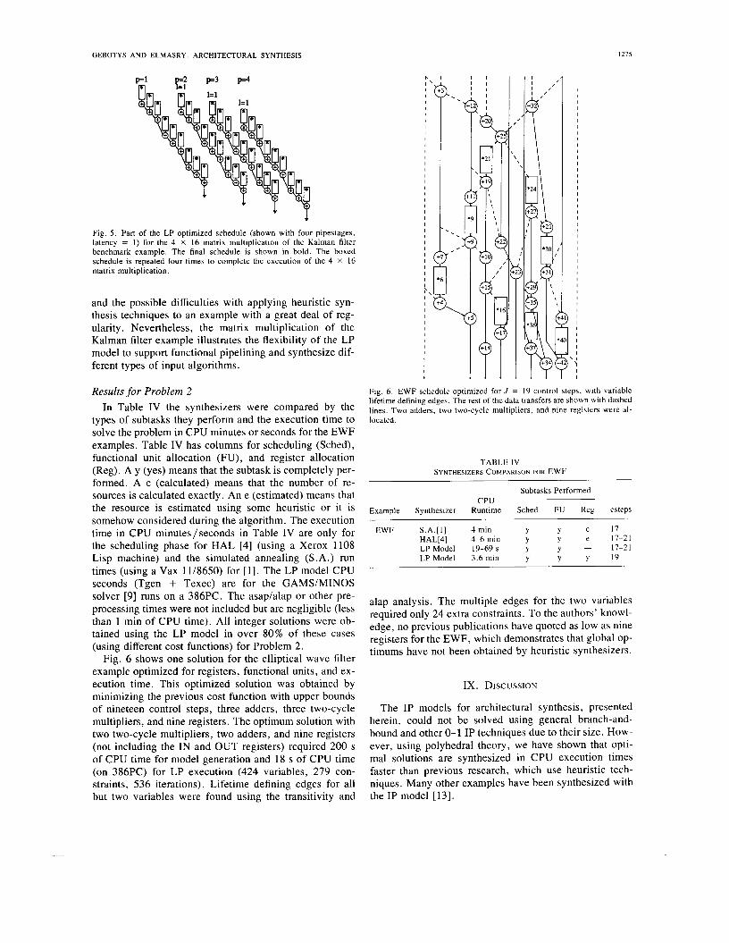
Fig. 6 shows one solution for the elliptical wave filter example optimized for registers, functional units, and execution time. This optimized solution was obtained by minimizing the previous cost function with upper bounds of nineteen control steps, three adders, three two-cycle multipliers, and nine registers. The optimum solution with two two-cycle multipliers, two adders, and nine registers (not including the IN and OUT registers) required 200 s of CPU time for model generation and 18 s of CPU time (on 386PC) for LP execution (424 variables, 279 constraints, 536 iterations). Lifetime defining edges for all but two variables were found using the transitivity and

I I I I I I I I I I I I I I I I I I I I I I I I I

I ( I I I I I I I I I I I I I

\ I

Fig. 6 . EWF schedule optimized for J = 19 control steps, with variable lifetime defining edges. The rest of the data transfers are shown with dashed lines. Two adders, two two-cycle multipliers, and nine registers were allocated.

TABLE IV SYNTHESIZERS COMPARISON FOR EWF

Subtasks Performed CPU

Example Synthesizer Runtime Sched FU Reg csteps

y c 17 EWF S.A.[l] 4 min Y HAL[4] 4-6 min y y e 17-21 LP Model 19-69 s y Y - 17-21 LP Model 3.6 min y Y Y 19

alap analysis. The multiple edges for the two variables required only 24 extra constraints. To the authors’ knowledge, no previous publications have quoted as low as nine registers for the EWF, which demonstrates that global op- timums have not been obtained by heuristic synthesizers.

IX. DISCUSSION

The IP models for architectural synthesis, presented herein, could not be solved using general branch-and- bound and other 0-1 IP techniques due to their size. How- ever, using polyhedral theory, we have shown that optimal solutions are synthesized in CPU execution times faster than previous research, which use heuristic techniques. Many other examples have been synthesized with the IP model [ 131.


If not all the variables in the solution are integers we can 1) automatically extract violated odd cycles facets using a shortest path algorithm [7], or 2) by solving the system of edge inequalities decompose the problem into a number of smaller ones to solve, or 3) branch and bound. These three techniques maintain optimality. Over 80% of the synthesized solutions (of the relaxed LP problem) optimized with different cost functions were all-integer. The cases where not all variables were integer mostly were a result of using objective functions which did not make practical sense for architectural synthesis applications.

Although the register allocation constraint (8) does not have the node packing structure, we have shown that we can still solve for integer variables in most cases and in very fast execution times. A different register allocation constraint, not presented herein, has the node packing structure (although it requires approximately double the variables) and, therefore, proves that simultaneous scheduling and allocation of functional units and registers is NP-complete by transformation to the node packing problem.

The worst case complexity for the IP problem in theory is exponential. This gives a poor representation of the expected complexity, since it means that there will be some problems that will take a long time to solve. However, similar to previous research [7], we have found that most problems are solved very fast, and it is expected that the majority will exhibit this behavior. As algorithms become larger, we intend to use the Karmarkar algorithm for LP solving [ 191, which executes ten times faster than the simplex and has shown larger improvements in speed as the problem size increases. Although we cannot guarantee 0-1 solutions (the problem is NP-complete), most examples we have optimized provide 0-1 solutions. For the first time, our IP model provides tight bounds on the architectural synthesis problem, which is extremely important for any synthesis solution technique, including simulated annealing or the use of techniques described herein.

A second approach for dealing with complexity relies on the designer to select subsets of the model to explore the design possibilities. For example, one can first minimize the number of functional units and then, second, minimize the number of registers to explore the architectural design space. There also exist various input algorithm partitioning strategies that have been researched to deal with complexity, such as vertical partitioning in [20] or partitioning and pipelining of the algorithm as demonstrated with the matrix multiplication example herein. However, more importantly, we have demonstrated that over 100 code operations can be simultaneously scheduled and allocated in very fast CPU times. This ability to optimally synthesize large complex algorithms is a significant contribution to the synthesis field.

The LP model presented herein is a set of general constraints and cost functions that can be used for any application. In other words, there is no need to extract new facets or formulate any new constraints to synthesize an architecture for each new application. Although we have

not specifically placed execution time in the objective function, our IP model can be extended easily to do this by adding an end operation (analogous to the end-of-loop operation) and placing it in the objective function similar to [21]. For example, the execution time can be formulated using an additional operation, end, where k < * end, V k , and Texec = E,,, ( ( j - l)~,,~~~,~). Then the cost function could model both area and delay. In addition, our IP model can be extended to support selection of chained functional units [13]. In this case, the designer can iden- tify what type of operations will be chained (e.g., k* < k + ) , and the iP model would use a fixed timing constraint in place of a precedence constraint for the operations that are assigned to the chained functional unit [time (k* , k , ) = 0 for all xLc,] ,k , where i, is a chained functional Unit, and k , < k , for all x,,,,~ where i # 4.1. The model can then simultaneously schedule, select, and allocate functional units.

X . CONCLUSIONS

Currently, we have formulated new models to simultaneously allocate interconnect [22] support asynchronous interfaces [23], select clock period [24], and partition into multichip architectures [25]. In the future, we intend to extend the LP model for simultaneous scheduling, allocation, and binding (to minimize the number of multiplexors and the number of inputs to multiplexors). We also plan to conduct additional research on the extraction of more facets and the use of this model for interfacing to analog signal processing domains.

The LP model presented herein is a significant contribution to the field of high-level architectural synthesis. For the first time, we have proof that the synthesized architectures are globally optimal. This is important for industry since the early decisions made during architectural exploration have the greatest impact on the final design. Previous synthesizers could at best guarantee a locally optimal synthesized solution, which may not meet design constraints. Finally, we have demonstrated that the IP architectural synthesizer can handle input algorithms with different types of structure, with over 100 code operations and with complex constraints. In summary, this research guarantees globally optimal synthesized solutions, syn- thesizes large input algorithms in practical execution times, and supports complex constraints and cost functions.

APPENDIX I: TIGHTER PRECEDENCE CONSTRAINT

Proof that constraint (5) is tighter than (5") is presented in this appendix. Let P5 represent the scheduling polytope whose constraint set is generated only by (5) and similarly for Ps*. This is equivalent to showing that P4 C P5*.

1) P5 # P5* Proof: Consider the following fractional solution to

GEBOTYS AND ELMASRY: ARCHITECTURAL SYNTHESIS 1277

the scheduling problem a , b ( a < * b, where the upper bound on the number of control steps is 4.

k ( j = l j = 2 j = 3 j = 4

0 .1

This solution is violated by ( 5 ) = ( ~ 3 , ~ + x 3 , b + x 2 . b ) = (.1) + ( . 5 ) + ( . 5 ) = 1 . 1 > 1 and feasible for (5*) =

= -1.3 I - 1. Therefore P5 # P5* Q.E.D.

a / b .9 .5 .5 0

C ; = l j x , , , - E j ” = 2 j ~ , , b = 1(.9) + 3(.1) - 2(.5) - 3( .5)

2 ) P5 P5*

n n

(a) (b)

Fig. 7. Example of facets forming the fixed timing constraint.

Proof:

&4, b

now we have to derive ( 5 * ) : x , , ~ + 2 x ~ , ~ + 3 x ~ , ~ - 2 X2,b - 3 X3,b - 4 X4,b I - 1 left-hand side Of ( 5 ” ) : 5 4 - 3 X2.b - 2 X 3 , b - X4,b - 2 ~ 2 , b - 3 X3,b - 4 X4,b (by substitution) = 4 - 5 (X2 ,b + x 3 , b + x 4 , J = -1.

Q.E.D. Since we have shown that P5 * P5* and P5 # P5*, we have proved that P5 C P5*. Thus ( 5 ) is a tighter formulation of the precedence constraint than ( 5 ” ) .

APPENDIX 11: EDGE REDUCTION ALGORITHM

The transitivity and alap analysis discussed in Section IV can be performed using the polynomial time algorithm described below in pseudocode.

Given the node-node adjacency matrix A i , j , where a i , j

= 1 e i < * j , where i, j are code operations. We will use this matrix to represent the DAG (or input algorithm). First a path matrix, T, is calculated. Second, the asap/ alap tables for each code operation and the path matrix are used to delete edges that cannot represent lifetimes.

1) Compute matrix T,j, where ti,, = 1 e 3 a path from code operation i to code operationj in the DAG.

2 ) Compute matrix Li,j, where l i , j = 1 edge i, j of the DAG cannot be eliminated by transitivity or alap analysis. Initially set L = A , and then eliminate entries V i,

v j i Y j 2 l a i , j , = ai,jz = 1. if((cjl,jz = 1) v ( a s a ~ ( j 2 )

I alap(j1))) * l i , j , = 0.

The algorithm is finished and the L matrix is used to generate the register constraints since each entry represents a possible lifetime defining edge.

APPENDIX 111: FACET PROOF FOR FIXED TIMING CONSTRAINTS

We will show that the fixed timing constraints inequalities (10) of Section VII, and the minimum/maximum timing constraints, inequalities (1 1) and (12) of Section

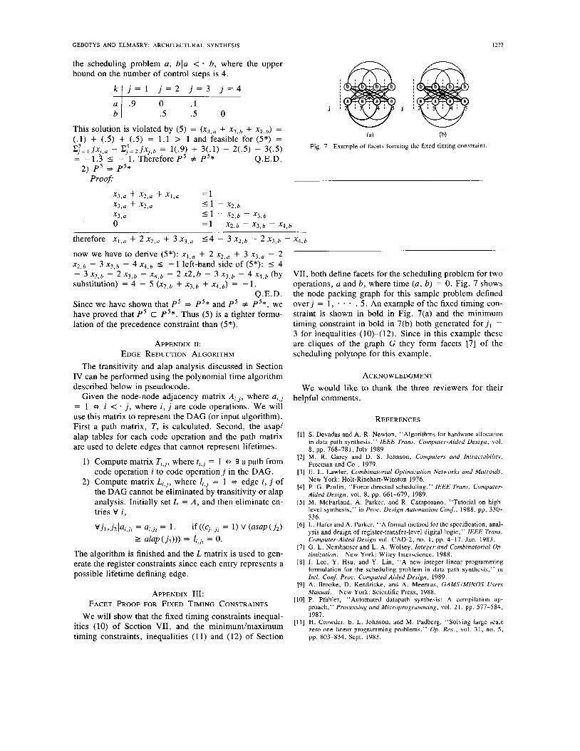
VII, both define facets for the scheduling problem for two operations, a and b, where time (a, b) = 0. Fig. 7 shows the node packing graph for this sample problem defined over j = 1 , * - - , 5 . An example of the fixed timing constraint is shown in bold in Fig. 7(a) and the minimum timing constraint in bold in 7(b) both generated f o r j , = 3 for inequalities (10)-(12). Since in this example these are cliques of the graph G they form facets [7] of the scheduling polytope for this example.

ACKNOWLEDGMENT We would like to thank the three reviewers for their

helpful comments.

REFERENCES

[ l ] S . Devadas and A. R. Newton, “Algorithms for hardware allocation in data path synthesis,” IEEE Trans. Computer-Aided Design, vol. 8, pp. 768-781, July 1989.

[2] M. R. Garey and D. S. Johnson, Computers and Intractability. Freeman and Co. , 1979.

[3] E. L. Lawler, Combinatorial Optimization Networks and Mutroids. New York: Holt-Rinehart-Winston 1976.

[4] P. G . Paulin, “Force directed scheduling,” IEEE Trans. Computer- Aided Design, vol. 8, pp. 661-679, 1989.

[5] M. McFarland, A. Parker, and R. Camposano, “Tutorial on high- level synthesis,” in Proc. Design Automation Conf., 1988, pp. 330- 336.

[6] L. Hafer and A. Parker, “A formal method for the specification, analysis and design of register-transfer-level digital logic,” IEEE Trans. Compurer-Aided Design vol. CAD-2, no. 1, pp. 4-17, Jan. 1983.

[7] G. L. Nemhauser and L. A. Wolsey, Integer and Combinatorial Op- timization. New York: Wiley Interscience, 1988.

[8] J . Lee, Y. Hsu, and Y. Lin, “A new integer linear programming formulation for the scheduling problem in data path synthesis,” in Intl. Con$. Proc. Computed Aided Design, 1989.

[9] A. Brooke, D. Kendricke, and A. Meeraus, GAMSIMINOS Users Manual.

[lo] P. Pfahler, “Automated datapath synthesis: A compilation approach,” Processing and Microprogramming, vol. 21, pp. 577-584, 1987.

[ l l ] H. Crowder, E. L. Johnson, and M. Padberg, “Solving large scale zero-one linear programming problems,” Op. Res. , vol. 31, no. 5 , pp. 803-834, Sept. 1983.

New York: Scientific Press, 1988.

IEEE TRANSACTIONS ON COMPUTER-AIDED DESIGN OF INTEGRATED CIRCUITS AND SYSTEMS, VOL. 12, NO. 9, SEPTEMBER 1993

K. R. Baker, Introduction to Sequencing and Scheduling. New York: Wiley, 1974. C. H . Gebotys, “A global optimization approach to architectural synthesis of VLSI Digital synchronous systems with analog and asynchronous interfaces,” Ph.D. thesis, Dept. ECE, University of Water- loo, July 1991. hlsw and B. Mayo (Coordinator), High-Level Synthesis Workshop Clearinghouse, email hlsw-request@decwrl. dec. com. 1988. C.-T. Hwang, J-H. Lee, and Y-C. Hsu, “A formal approach to the scheduling problem in high-level synthesis,” IEEE Trans. Computer- Aided Design, vol. CAD-IO, no. 4 , pp. 464-475, 1991. A. Parker, “Tutorial on high level synthesis,” in Can. Conf. on VLSI, 1991. R. Camposano, “Path based scheduling for synthesis,” IEEE Trans. Computer-Aided Design, vol. CAD-10, pp. 85-93, 1991. E. D. Lagnese, “Architectural partitioning for systems level design of integrated circuits,” Ph.D. thesis, CMUCAD-89-27, Carnegie- Mellon University, Pittsburgh, PA, 1989. N. Karmarkar, “A new polynomial time algorithm for linear programming,” Combinatorica, vol. 4 , pp. 373-395, 1984. F. Depuydt, G. Goossens, J . Van Meerbergen, F. Catthoor, and H. DeMan, “Scheduling of large scale signal flow graphs based on met- ric graph clustering, ” in IFIP Con$ High Level Architectural Synthe- sis and Logic Synthesis, 1990. C. H. Gebotys and M. I. Elmasry, “Simultaneous scheduling and allocation for cost constrained optimal architectural synthesis, ” in ACMilEEE Design Automation Conf. , 1991. C. H . Gebotys and M. I . Elmasry, “Optimal synthesis of high-performance architectures,” IEEE J . Solid-State Circuit, vol. SC-2, no.

C. H. Gebotys, “Synthesizing embedded speed-optimized architectures,” in IEEE Custom Integrated Circuits Conf., pp. 8.7.1-8.7.4, 1992. C. H. Gebotys, “Optimal scheduling and allocation of embedded VLSI chips,” in ACMilEEE Design Automation Conf., 1992. C. H . Gebotys, “Optimal synthesis of multichip architectures,’’ in IEEEIACM Int. Conf. CAD, 1992.

3 , p p . 389-397, 1992.

Catherine H. Gebotys (S’82-M’92) received the B.A.Sc. degree in engineering science in 1982 and the M.A.Sc. degree in electrical engineering in 1984, both from the University of Toronto, On- tario, Canada. She received the Ph.D. degree in electrical engineering in 1991 from the University of Waterloo, Ontario, Canada.

She worked at Litton Systems Canada Ltd., Display Systems Engineering, from January 1985 to December 1986, in the area of CAD for VLSI and chip design. From January 1987 to August

1989, she was a research associate in the VLSI Group, Department of Elec- trical Engineering, University of Waterloo. She has been Assistant Profes- sor in the Department of Electrical and Computer Engineering, University of Waterloo since September 1991. She is coauthor of the book Optimal VLSI Architectural Synthesis: Area, Performance and Testability, Kluwer Academic Publishers, 1992. Her research interests include global optimization approaches to CAD for VLSI, high-level architectural synthesis, and design for test.

Mohamed I. Elmasry received the B.Sc. degree from Cairo University, Cairo, Egypt, and the M.A.Sc. and Ph.D. degrees from the University of Ottawa, Ontario, Canada, all in electrical engineering in 1965, 1970, and 1974, respectively.

He has worked in the area of digital integrated circuits and system design for the last 25 years. He worked for Cairo University from 1965 to 1968 and for Bell-Northern Research, Ottawa, Canada, from 1972 to 1974. He has been with the Depart- ment of Electrical and Computer Engineering,

University of Waterloo, since 1974, where he is a Professor and founding director of the VLSI research group. He has a cross appointment with the Department of Computer Science, where he is a Professor. He holds the NSERCiBNR Research Chair in VLSI design at the same university since 1986. He has served as a consultant to research laboratories in Canada and the United States, including AT&T Bell Labs, GE, CDC, Ford Microelec- tronics, Linear Technology, Xerox, and BNR, in the area of LSIiVLSI digital circuitisubsystem design. During sabbatical leaves from Waterloo he was at the Micro Component Organization, Burroughs Corporation (Un- isys), San Diego, CA, Kuwait University, Kuwait, and Swiss Federal In- stitute of Technology, Lausanne, Switzerland. He has authored and coau- thored over 150 papers on integrated circuit design and design automation. He has several patents to his credit. He is the editor of the IEEE Press books Digital MOS Integrated Circuits, 1981, Digital VLSI Sysrems, 1985, and Digital MOS Integrated Circuits 11, 1991. He is also author of the book Digital Bipolar Integrated Circuits (Wiley, 1983) and coauthor of the book Digital BiCMUS Inregrured Circuits (Kluwer, 1991). Dr. Elmasry has served in many professional organizations in different positions including the Chairmanship of the Technical Advisory Committee of the Canadian Microelectronics Corporation. He is a founding member of the Canadian VLSI Conference, the International Conference on Microelectronics and the founding president of Pic0 Electronics Inc.

Dr. Elmasry is a member of the Association of Professional Engineers of Ontario and is a Fellow of the IEEE for his contributions to digital integrated circuits.

A Global Optimization Approach for Architectural Synthesis

Documents

Transcript of A Global Optimization Approach for Architectural Synthesis