http://pii.sagepub.com/Control Engineering

Engineers, Part I: Journal of Systems and Proceedings of the Institution of Mechanical

http://pii.sagepub.com/content/223/6/753The online version of this article can be found at:

 DOI: 10.1243/09596518JSCE789

2009 223: 753Proceedings of the Institution of Mechanical Engineers, Part I: Journal of Systems and Control EngineeringJ Roshanian, M Zareh, H H Afshari and M Rezaei

adaptive closed-loop guidance law for an orbital injection problem1An L  

Published by:

http://www.sagepublications.com

On behalf of: 

  Institution of Mechanical Engineers

can be found at:EngineeringProceedings of the Institution of Mechanical Engineers, Part I: Journal of Systems and ControlAdditional services and information for

    

  http://pii.sagepub.com/cgi/alertsEmail Alerts:

 

http://pii.sagepub.com/subscriptionsSubscriptions:  

http://www.sagepub.com/journalsReprints.navReprints:  

http://www.sagepub.com/journalsPermissions.navPermissions:  

http://pii.sagepub.com/content/223/6/753.refs.htmlCitations:  

by guest on July 12, 2011pii.sagepub.comDownloaded from

An L1 adaptive closed-loop guidancelaw for an orbital injection problemJ Roshanian, M Zareh*, H H Afshari, and M Rezaei

Department of Aerospace Engineering, K.N. Toosi University of Technology, Tehran, Iran

The manuscript was received on 12 April 2009 and was accepted after revision for publication on 11 June 2009.

DOI: 10.1243/09596518JSCE789

Abstract: The current paper presents the determination of a closed-loop guidance law for anorbital injection problem using two different approaches and, considering the existing time-optimal open-loop trajectory as the nominal solution, compares the advantages of the twoproposed strategies. In the first method, named neighbouring optimal control (NOC), theperturbation feedback method is utilized to determine the closed-loop trajectory in ananalytical form for the non-linear system. This law, which produces feedback gains, is ingeneral a function of small perturbations appearing in the states and constraints separately.The second method uses an L1 adaptive strategy in determination of the non-linear closed-loop guidance law. The main advantages of this method include characteristics such asimprovement of asymptotic tracking, guaranteed time-delay margin, and smooth controlinput. The accuracy of the two methods is compared by introducing a high-frequencysinusoidal noise. The simulation results indicate that the L1 adaptive strategy has a betterperformance than the NOCmethod to track the nominal trajectory when the noise amplitude isincreased. On the other hand, the main advantage of the NOC method is its ability to solve anon-linear, two-point, boundary-value problem in the minimum time.

Keywords: L1 adaptive control, optimal control, optimal guidance

1 INTRODUCTION

Optimal formulations of non-linear dynamic sys-

tems, either through dynamic programming or

variational approaches, lead to non-linear partial

differential equations. Numerical solution of such

equations dealing with complex non-linear systems

is always difficult, especially for real-world physical

problems. Obtaining closed-loop control laws in-

tensifies the inherent difficulty involved and is only

exceptionally determined in some rare cases. Be-

sides, open-loop control laws, dependent on initial

conditions, are highly sensitive to noise and external

disturbances and therefore are not preferred for real-

world applications. On the contrary, closed-loop

control policies are desirable owing to their natural

robustness to perturbations. In addition, there exist

certain difficulties associated with the numerical

determination of open-loop optimal control solu-

tions for non-linear systems, such as slow conver-

gence rate and high sensitivity to initial guessti-

mates.

The technique of neighbouring optimal control

(NOC) produces time-variant feedback control that

minimizes a performance index to second order for

perturbation from a nominal optimal path. Pertur-

bations in the nominal optimal states are compen-

sated for, but errors in the system dynamic model

parameters, such as mass variation and environment

disturbance, may substantially affect the perfor-

mance. Also, the neighbouring extremals are given

for orbital injection [1]. The time-optimal solution of

a non-linear landing mission in polar coordinates

was investigated utilizing a numerical technique

named linear programming. This law is an exact

solution to the two-point boundary-value problem

associated with the necessary conditions for first

variation [2]. The results of minimum-time feedback

laws [3] are used to validate the results of an

*Corresponding author: Department of Aerospace Engineering,

K.N. Toosi University of Technology, East Vafadar Street, 4th

Tehranpars Square, Tehran 1656983211, Iran.

email: mehranzareh@aol.com

753

JSCE789 Proc. IMechE Vol. 223 Part I: J. Systems and Control Engineering

by guest on July 12, 2011pii.sagepub.comDownloaded from

analytical open-loop strategy proposed in the present

paper. Jardin and Bryson used the technique of NOC

to develop an algorithm for optimizing aircraft tra-

jectories in general wind fields by computing time-

varying linear feedback gains [4, 5]. Furthermore,

Pourtakdoust et al. presented a time-optimal open-

loop strategy for a non-linear lunar landing mission

using an analytical technique. To create closed-loop

fuzzy guidance logic, a fuzzy algorithm was augmen-

ted to the variational function of the problem [6, 7].

Palma and Magni have worked on optimal predictive

control by discretizing non-linear dynamic systems

[8]. Recently, Afshari et al. employed analytical

approaches to obtain non-linear optimal guidance

policies of spacecraft missions [9, 10].

There are many reasons why researchers prefer

adaptive laws to find control signals, especially for

non-linear problems for which an analytical solution

is barely possible. Uncertainties in the system,

disturbances, and measurement noise are some of

these reasons. The L1 adaptive strategy has recently

been introduced by Cao and Hovakimyan [11–13].

This new approach presents much better results,

especially during the transient phase. As proved

previously, it can provide robust performance

against external disturbances and measurement

noises. The other advantages of L1 adaptive archi-

tecture, such as improved asymptotic tracking and

guaranteed time-delay margin, achieved via smooth

control input, have also been discussed previously.

The L1 adaptive control approach replaces the

conventional model reference adaptive control

(MRAC) by first specifying an equivalent companion

model architecture, which enables insertion of a

low-pass filter in the closed loop. To ensure

asymptotic stability of the closed-loop system, the

L1 gain of the cascaded system involving the low-

pass filter and the desired closed-loop reference

system needs to be less than the inverse of the upper

bound on the unknown parameters used in the

projection-type adaptation law [14–18]. The present

study demonstrates the first usage of L1 adaptive

control in the determination of a closed-loop

guidance law for spacecraft missions. For this

purpose, the selected companion model should

track the optimal trajectory with the optimal control

signal considered as the reference input. To have a

smooth input signal, a low-pass filter is utilized by

satisfying the L1 small gain theorem [19–21].

2 OPEN- VERSUS CLOSED-LOOP SOLUTION

Optimal control of non-linear dynamic systems will

typically be of open-loop type, usually determined as

a function of time, u(t). An optimal control policy is

designed to move the system from its initial state

x(0) towards the specified terminal hypersurface,

y xtf ,tf� �

~0, in a manner that minimizes the cost

function. In this sense any point on the computed

trajectory from [x(t0),t0] to the terminal hypersurface

could be a possible initial point for which optimal

control is already at hand, but for other initial points

not lying on the predetermined trajectory, the

current policy would no longer be optimal and the

problem must be solved again. Bearing in mind the

open-loop nature of the control history in non-linear

optimal control problems, one can easily justify the

need for many solutions linked to various initial

conditions. To overcome this problem, a family of

optimal trajectories is needed to envelop all of the

feasible initial conditions, a task not easily accom-

plished. Generally speaking, for each initial condi-

tion [x(t0),t0] there exists an optimal trajectory to

arrive at the specified target hypersurface. The

corresponding control history u0(t) can be expressed

as

u0~u0 x,tð Þ ð1Þ

which is now in the so-called closed-loop form. This

means that the optimal control action is a function

of state x(t) and current time t. For a stationary

system having performance measures and con-

straints that are not explicit functions of time, the

optimal control will also be an implicit function of

time, namely

u0~u0 xð Þ ð2Þ

However, determination of closed-loop optimal

control policies for non-linear systems is a formid-

able task. Moreover, if one desires the advantages

associated with closed-loop policies, simplifying

assumptions must be made to linearize the system

around some working conditions [6].

3 OPEN-LOOP SOLUTION TO THE SPACECRAFTINJECTION PROBLEM

In this section, the results of an analytical time-

optimal solution obtained for a spacecraft injection

mission are utilized. In this way, consider an

idealized spacecraft at the origin of inertial frame

(x,y) at t5 0, moving under the action of a constant

propulsive force making a control angle b with the

horizon. Obviously, the position and velocity vector

of the vehicle will change due to the forces acting

754 J Roshanian, M Zareh, H H Afshari, and M Rezaei

Proc. IMechE Vol. 223 Part I: J. Systems and Control Engineering JSCE789

by guest on July 12, 2011pii.sagepub.comDownloaded from

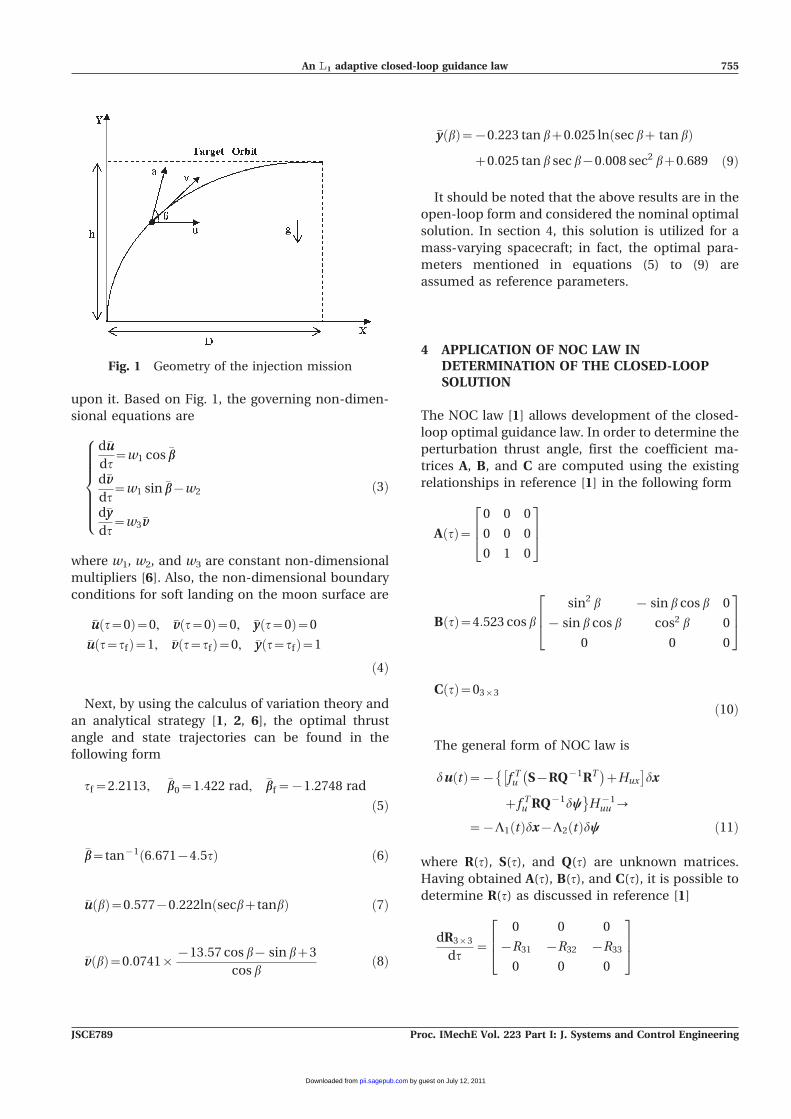
upon it. Based on Fig. 1, the governing non-dimen-

sional equations are

d�uu

dt~w1 cos �bb

d�vv

dt~w1 sin �bb{w2

d�yy

dt~w3�vv

8>>>>>><>>>>>>:

ð3Þ

where w1, w2, and w3 are constant non-dimensional

multipliers [6]. Also, the non-dimensional boundary

conditions for soft landing on the moon surface are

�uu t~0ð Þ~0, �vv t~0ð Þ~0, �yy t~0ð Þ~0

�uu t~tfð Þ~1, �vv t~tfð Þ~0, �yy t~tfð Þ~1

ð4Þ

Next, by using the calculus of variation theory and

an analytical strategy [1, 2, 6], the optimal thrust

angle and state trajectories can be found in the

following form

tf~2:2113, �bb0~1:422 rad, �bbf~{1:2748 rad

ð5Þ

�bb~tan{1 6:671{4:5tð Þ ð6Þ

�uu bð Þ~0:577{0:222ln secbztanbð Þ ð7Þ

�vv bð Þ~0:0741|{13:57 cos b{ sin bz3

cos bð8Þ

�yy bð Þ~{0:223 tan bz0:025 ln sec bz tan bð Þz0:025 tan b sec b{0:008 sec2 bz0:689 ð9Þ

It should be noted that the above results are in the

open-loop form and considered the nominal optimal

solution. In section 4, this solution is utilized for a

mass-varying spacecraft; in fact, the optimal para-

meters mentioned in equations (5) to (9) are

assumed as reference parameters.

4 APPLICATION OF NOC LAW INDETERMINATION OF THE CLOSED-LOOPSOLUTION

The NOC law [1] allows development of the closed-

loop optimal guidance law. In order to determine the

perturbation thrust angle, first the coefficient ma-

trices A, B, and C are computed using the existing

relationships in reference [1] in the following form

A tð Þ~0 0 0

0 0 0

0 1 0

264

375

B tð Þ~4:523 cos b

sin2 b { sin b cos b 0

{ sin b cos b cos2 b 0

0 0 0

264

375

C tð Þ~03|3

ð10Þ

The general form of NOC law is

du tð Þ~{ f Tu S{RQ{1RT� �

zHux

� ��dx

zf Tu RQ{1dy�H{1

uu ?

~{L1 tð Þdx{L2 tð Þdy ð11Þ

where R(t), S(t), and Q(t) are unknown matrices.

Having obtained A(t), B(t), and C(t), it is possible to

determine R(t) as discussed in reference [1]

dR3|3

dt~

0 0 0

{R31 {R32 {R33

0 0 0

264

375

Fig. 1 Geometry of the injection mission

An L1 adaptive closed-loop guidance law 755

JSCE789 Proc. IMechE Vol. 223 Part I: J. Systems and Control Engineering

by guest on July 12, 2011pii.sagepub.comDownloaded from

R tfð Þ~I3|3 ð12Þ

Each member of the matrix equation (12) forms a

differential equation that must be integrated back-

wards from the terminal time to the current time.

Due to the fact that the thrust angle b(t) is related to

time, the matrix Q(t) can be easily determined by

solving a set of independent differential equations

with corresponding boundary conditions in the

following form

Therefore, Q(t) is obtained analytically by backward

integration from each member of matrix differential

equation (13) with respect to time. In effect, the

differential equations are swept backwards from the

terminal condition to the current condition in the

exact solution.

Since the co-state equations are not functions of

state variables, the matrix S(t) is equal to zero and

solving the Riccati equation is not required. Note

that because the spacecraft injection problem is in

the class of a terminal guidance problem, the

perturbation on terminal constraints will be equal

to zero. As a result, the NOC law is a function of

perturbation on state variables only. The NOC block

diagram for determining the optimal closed-loop

control law for the spacecraft injection problem is

depicted in Fig. 2. Also, by computing the time

perturbation, it is found to be less than 1023, so that

it is negligible. By regarding the previous relation-

ships, the NOC law can be applied in the following

formulation

db tð Þ~Ku tð Þdu tð ÞzKv tð Þdv tð ÞzKy tð Þdy tð Þ ð14Þ

where the perturbed terms du(t), dv(t), and dy(t) are

small perturbations applied to the state variables of

the spacecraft injection system, and Ku(t), Kv(t), and

Ky(t) are neighbouring optimum gains for determi-

nation of the optimal closed-loop guidance law.

5 USING THE L1 ADAPTIVE APPROACH TOREACH A CLOSED-LOOP OPTIMAL GUIDANCE

MRAC is one of the main approaches for adaptive

control. The reference model is chosen to generate

the desired trajectory ym that the plant output yp has

to follow. The closed-loop plant is made up of an

ordinary feedback control law that contains the

plant, a controller C(h), and an adjustment mechan-

ism that generates the controller parameter esti-

mates h(t) on-line. It is possible to ensure that the

input and output of an uncertain linear system track

the input and output of a desired linear system

during the transient phase, in addition to the

asymptotic tracking, by using the L1 adaptive

approach. These features are established by first

performing an equivalent re-parametrization of

MRAC, the key difference of which with respect to

MRAC is in the definition of the error signal for

dQ3|3

dt~4:523 cos b|

sin2 b { sin b cos b { tf{tð Þ sin b cos b

{ sin b cos b cos2 b tf{tð Þ cos2 b{ tf{tð Þ sin b cos b tf{tð Þ cos2 b tf{tð Þ2cos2 b

264

375

Q tfð Þ~03|3

ð13Þ

Fig. 2 Block diagram of the NOC law for design of theclosed-loop trajectory

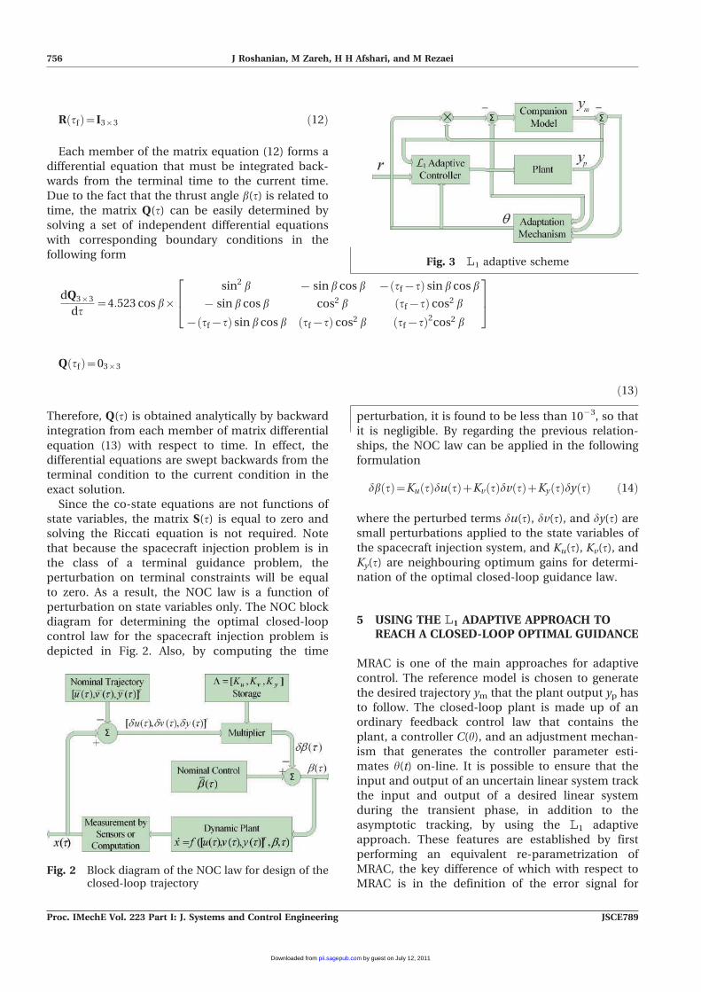
Fig. 3 L1 adaptive scheme

756 J Roshanian, M Zareh, H H Afshari, and M Rezaei

Proc. IMechE Vol. 223 Part I: J. Systems and Control Engineering JSCE789

by guest on July 12, 2011pii.sagepub.comDownloaded from

adaptive laws. This new architecture, called the

companion model adaptive controller (CMAC),

allows for incorporation of a low-pass filter into the

feedback loop that enables one to enforce the

desired transient performance by increasing the

adaptation gain [12]. A block diagram of this method

is shown in Fig. 3. To describe the idea, consider an

imaginary spacecraft parallel to a real one that with

an optimal control signal produces an optimal

trajectory. So if the adaptation mechanism is able

to reduce the tracking error e5 yp2 ym to zero, then

the real spacecraft will behave like the imaginary one

and so will track the optimal trajectory. By reformu-

lating equation (3) we have

_XX~f X ,bð Þ ð15Þ

where X5 [u v y]. Now consider the following

reference model dynamics that satisfies the optimal

trajectory

_XXm~f � Xm,bcð Þ ð16Þ

where Xm5 [um vm ym] and bc is not like that of

conventional MRAC, being defined by a CMAC

structure as follows

bc~b{hTX ð17Þ

The aim of L1 adaptive control is to find b as a

function of states such that the input and output of

the system track the input and output of a desired

system during the transient phase, in addition to the

asymptotic tracking. To reach this end, a low-pass

filter is added to the control signal

b~FLP b�zhTX� � ð18Þ

where FLP{b* + hTX} denotes a low-pass filter. The

vector h contains adaptation parameters. By defining

deviation between the real output and the desired

output as

e~Xm{X ð19Þ

gives

_ee~f � Xm,bcð Þ{f X ,bð Þ ð20Þ

Let the adaptation parameters vector be such that

f~sf � ð21Þ

where

s~

h1 0 0

0 h2 0

0 0 h3

264

375

If the error goes to zero then it is clear that

h5 [1,1,1]T. So we define

h�~ 1,1,1½ �T

By this definition one can obtain from equation (20)

that

_ee~ I{sð Þf �

in which I363 is the unique matrix. Now matrices

A363 and B361 are defined so that A is Hurwitz, (A, B)

is controllable, and

_ee~AezB XT~hh� � ð22Þ

where h5 h2 h*. Consider the Lyapunov function as

follows

V~1

2ePez

~hhT~hh

c

!ð23Þ

where P is a 363 matrix and c is a real constant

scalar. To have a stable system dv/dt must be

negative. Differentiating from equation (23), one

obtains ATP +PA52Q in which Q is positive definite

and

_hh~{cProj e,XBTP� � ð24Þ

Proj(?) denotes the projection operator [22].

6 RESULTS AND DISCUSSION

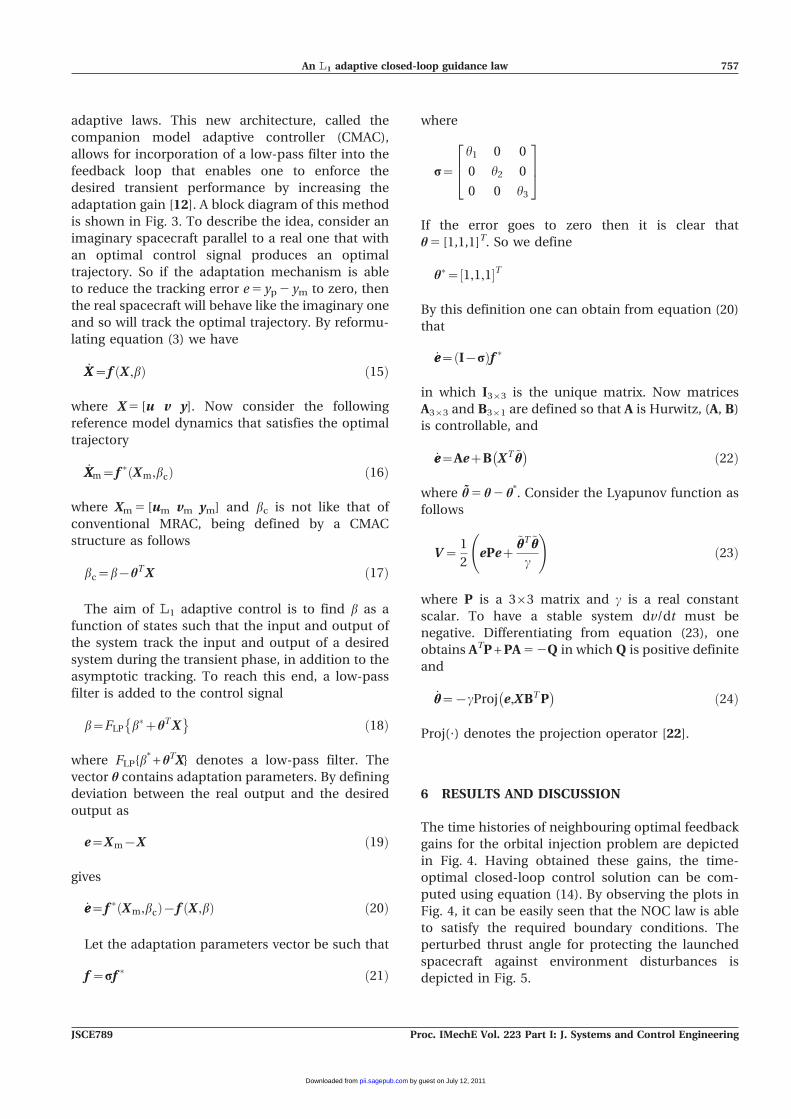
The time histories of neighbouring optimal feedback

gains for the orbital injection problem are depicted

in Fig. 4. Having obtained these gains, the time-

optimal closed-loop control solution can be com-

puted using equation (14). By observing the plots in

Fig. 4, it can be easily seen that the NOC law is able

to satisfy the required boundary conditions. The

perturbed thrust angle for protecting the launched

spacecraft against environment disturbances is

depicted in Fig. 5.

An L1 adaptive closed-loop guidance law 757

JSCE789 Proc. IMechE Vol. 223 Part I: J. Systems and Control Engineering

by guest on July 12, 2011pii.sagepub.comDownloaded from

There are several source of noise or disturbance in

the operating environment that affect the perfor-

mance of the determined optimal feedback laws. To

investigate the robustness potentials of these two

methods, i.e. NOC and L1 adaptive laws, the pro-

blem dynamic system is analysed under the influ-

ence of small disturbances exerted on the state

feedback (measurement unit) of the system. These

state disturbances, modelled similar to the control

actuation noise, are taken as

j tð Þ~e sin vtð Þ ð25Þ

and

�uuj~�uuzj tð Þ, �vvj~�vvzj tð Þ ð26Þ

where the noise frequency is v15 250. The design

parameters of the L1 adaptive controller are chosen

as follows

P~{1

2

1 0 0

0 1 0

0 0 1

2664

3775, A~

{1 0 0

0 {1 0

0 0 {1

2664

3775,

B~

1

1

1

26643775

c~3 and FLP~400

sz400

Limitation of the adaptation parameters is defined as

hj j¡hmax~10

To compare the robustness potentials of each

method, two scenarios are designed. In the first, a

sinusoidal noise with 0.01 amplitude is applied to

the dynamic system; therefore e5 0.01. Thereafter,

the closed-loop solutions of the two methods are

computed. In the other scenario, the amplitude of

the sinusoidal noise is taken as 0.1, i.e. e5 0.10.

Comparisons between the NOC and L1 adaptive

results are illustrated in Figs 6 to 13.

As can be seen in Figs 6 to 9, when the noise

amplitude is equal to 0.01, an excellent agreement

Fig. 4 Neighbouring optimum gains for the spacecraftinjection mission

Fig. 5 Perturbed thrust angle, due to applying dis-turbance, obtained using the NOC law

Fig. 6 Comparison between NOC and L1 closed-loopsolutions for thrust angle (e5 0.01)

758 J Roshanian, M Zareh, H H Afshari, and M Rezaei

Proc. IMechE Vol. 223 Part I: J. Systems and Control Engineering JSCE789

by guest on July 12, 2011pii.sagepub.comDownloaded from

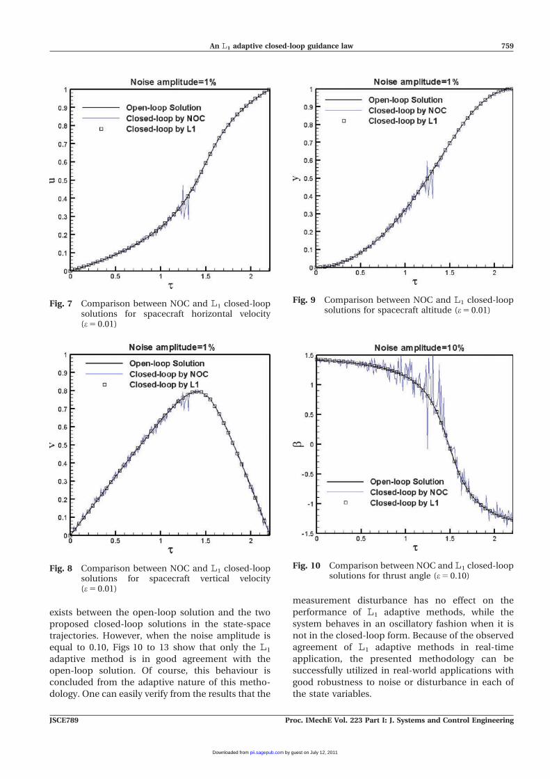
exists between the open-loop solution and the two

proposed closed-loop solutions in the state-space

trajectories. However, when the noise amplitude is

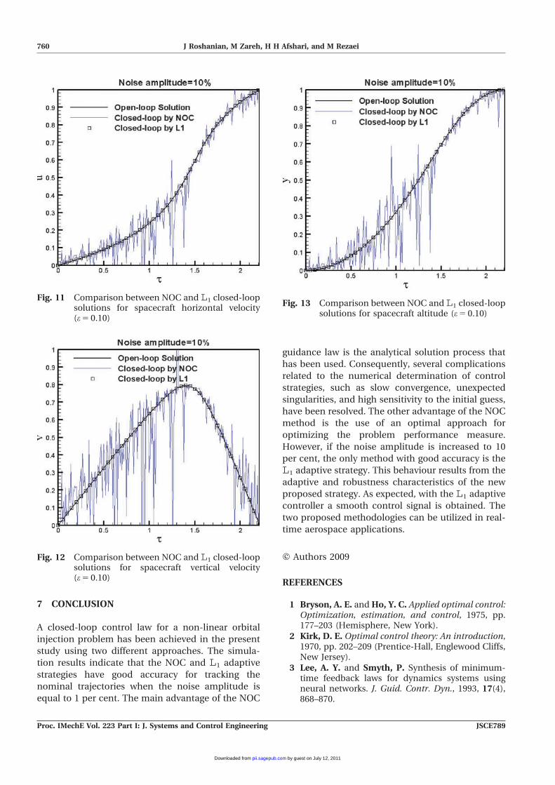
equal to 0.10, Figs 10 to 13 show that only the L1

adaptive method is in good agreement with the

open-loop solution. Of course, this behaviour is

concluded from the adaptive nature of this metho-

dology. One can easily verify from the results that the

measurement disturbance has no effect on the

performance of L1 adaptive methods, while the

system behaves in an oscillatory fashion when it is

not in the closed-loop form. Because of the observed

agreement of L1 adaptive methods in real-time

application, the presented methodology can be

successfully utilized in real-world applications with

good robustness to noise or disturbance in each of

the state variables.

Fig. 7 Comparison between NOC and L1 closed-loopsolutions for spacecraft horizontal velocity(e5 0.01)

Fig. 8 Comparison between NOC and L1 closed-loopsolutions for spacecraft vertical velocity(e5 0.01)

Fig. 9 Comparison between NOC and L1 closed-loopsolutions for spacecraft altitude (e5 0.01)

Fig. 10 Comparison between NOC and L1 closed-loopsolutions for thrust angle (e5 0.10)

An L1 adaptive closed-loop guidance law 759

JSCE789 Proc. IMechE Vol. 223 Part I: J. Systems and Control Engineering

by guest on July 12, 2011pii.sagepub.comDownloaded from

7 CONCLUSION

A closed-loop control law for a non-linear orbital

injection problem has been achieved in the present

study using two different approaches. The simula-

tion results indicate that the NOC and L1 adaptive

strategies have good accuracy for tracking the

nominal trajectories when the noise amplitude is

equal to 1 per cent. The main advantage of the NOC

guidance law is the analytical solution process that

has been used. Consequently, several complications

related to the numerical determination of control

strategies, such as slow convergence, unexpected

singularities, and high sensitivity to the initial guess,

have been resolved. The other advantage of the NOC

method is the use of an optimal approach for

optimizing the problem performance measure.

However, if the noise amplitude is increased to 10

per cent, the only method with good accuracy is the

L1 adaptive strategy. This behaviour results from the

adaptive and robustness characteristics of the new

proposed strategy. As expected, with the L1 adaptive

controller a smooth control signal is obtained. The

two proposed methodologies can be utilized in real-

time aerospace applications.

F Authors 2009

REFERENCES

1 Bryson, A. E. andHo, Y. C. Applied optimal control:Optimization, estimation, and control, 1975, pp.177–203 (Hemisphere, New York).

2 Kirk, D. E. Optimal control theory: An introduction,1970, pp. 202–209 (Prentice-Hall, Englewood Cliffs,New Jersey).

3 Lee, A. Y. and Smyth, P. Synthesis of minimum-time feedback laws for dynamics systems usingneural networks. J. Guid. Contr. Dyn., 1993, 17(4),868–870.

Fig. 11 Comparison between NOC and L1 closed-loopsolutions for spacecraft horizontal velocity(e5 0.10)

Fig. 12 Comparison between NOC and L1 closed-loopsolutions for spacecraft vertical velocity(e5 0.10)

Fig. 13 Comparison between NOC and L1 closed-loopsolutions for spacecraft altitude (e5 0.10)

760 J Roshanian, M Zareh, H H Afshari, and M Rezaei

Proc. IMechE Vol. 223 Part I: J. Systems and Control Engineering JSCE789

by guest on July 12, 2011pii.sagepub.comDownloaded from

4 Jardin, M. R. and Bryson, A. E. Neighboringoptimal aircraft guidance in winds. J. Guid. Contr.Dyn., 2001, 24(4), 710–715.

5 Lee, A. Y. and Bryson, A. E. Neighboring extremalsof dynamic optimization problems with parametervariations. Optim. Contr. Appl. Meth., 1989, 10(1),39–52.

6 Pourtakdoust, S. H., Rahbar, N., and Novinzadeh,A. B. Nonlinear feedback optimal control law forminimum-time injection problem using fuzzysystem. Aircraft Engng Aerospace Technol., 2005,77(5), 376–383.

7 Chun-Liang, L., Yu-Ping, L., and Tian-Lin, W. Afuzzy guidance law for vertical launch interceptors.Control Engng Practice, 2009, 17(8), 914–923.

8 Palma, D. and Magni, L. On optimality of non-linear model predictive control. Syst. Contr. Lett.,2005, 5(6), 58–61.

9 Afshari, H. H., Roshanian, J., and Novinzadeh,A. B. A perturbation approach in determination ofa closed-loop optimal-fuzzy control policy forplanetary landing mission. Proc. IMechE, Part G: J.Aerospace Engineering, 2009, 223(G3), 233–243.DOI: 10.1243/09544100JAERO429.

10 Afshari, H. H., Zareh, M., Rezaei, M., Roshanian,J., and Novinzadeh, A. B. A new adaptive approachin determination of closed-loop guidance law forinjection problem. In Proceedings of the 2009 IEEEAerospace conference, Big Sky, Montana, 7–14March 2009, p. 1705 (International AstronauticalFederation, Paris).

11 Cao, C. and Hovakimyan, N. Design and analysisof a novel L1 adaptive control architecture, Part 1:Control signal and asymptotic stability. In Proceed-ings of the 2006 American control conference,Minneapolis, Minnesota, 14–16 June 2006, pp.3397–3402 (Institute of Electrical and ElectronicsEngineers, Piscataway, New Jersey).

12 Cao, C. and Hovakimyan, N. Design and analysisof a novel L1 adaptive controller, Part 2: Guaran-teed transient performance. In Proceedings of the2006 American control conference, Minneapolis,Minnesota, 14–16 June 2006, pp. 3403–3408 (In-stitute of Electrical and Electronics Engineers,Piscataway, New Jersey).

13 Cao, C. and Hovakimyan, N. Guaranteed transientperformance with L1 adaptive controller for sys-tems with unknown time-varying parameters and

bounded disturbance: Part 2. In Proceedings of the2007 American control conference, New York, NewYork, 9–13 July 2007, pp. 3925–3930 (Institute ofElectrical and Electronics Engineers, Piscataway,New Jersey).

14 Beard, W. R., Knoebel, N., Cao, C., Hovakimyan,N., and Matthews, J. An L1 adaptive pitch con-troller for miniature air vehicles. AIAA Guidance,Navigation, and Control Conference, AIAA paper2006-6777, 2006.

15 Slotine, J. J. and Li, W. Applied nonlinear control,1991 (Prentice Hall, Englewood Cliffs, New Jersey).

16 Astrom, K. and Wittenmark, B. Adaptive control,edition 2, 1995 (Addison Wesley, Reading, Massa-chusetts).

17 Cao, C. and Hovakimyan, N. Novel L1 neuralnetwork adaptive control architecture with guar-anteed transient performance. IEEE Trans. NeuralNetwork., 2007, 18(4), 1160–1171.

18 Wang, J., Cao, C., Hovakimyan, N., and Lavretsky,E. Novel L1 adaptive control approach to autono-mous aerial refueling with guaranteed transientperformance. In Proceedings of the 2006 Americancontrol conference, Minneapolis, Minnesota, 14–16June 2006, pp. 3569–3574 (Institute of Electricaland Electronics Engineers, Piscataway, New Jer-sey).

19 Cao, C. and Hovakimyan, N. Stability margins ofL1 adaptive controller. In Proceedings of the 2007American control conference, New York, New York,9–13 July 2007, pp. 3931–3936 (Institute of Elec-trical and Electronics Engineers, Piscataway, NewJersey).

20 Cao, C., Patel, V., Reddy, C. K., Hovakimyan, N.,and Lavretsky, E. Are the phase and time-delaymargins always adversely affected by high-gain?AIAA Guidance, Navigation, and Control Confer-ence, AIAA paper 2006-6347, 2006.

21 Wang, J., Patel, V. V., Cao, C., Hovakimyan, N.,and Lavretsky, E. L1 adaptive neural networkcontroller for autonomous aerial refueling withguaranteed transient performance. AIAA Guidance,Navigation, and Control Conference, AIAA paper2006-6206, 2006.

22 Pomet, J. and Praly, L. Adaptive nonlinear regula-tion: estimation from the Lyapunov equation. IEEETrans. Automat. Contr., 1992, 37(6), 729–740.

An L1 adaptive closed-loop guidance law 761

JSCE789 Proc. IMechE Vol. 223 Part I: J. Systems and Control Engineering

by guest on July 12, 2011pii.sagepub.comDownloaded from