DryadeParent, An Efficient and Robust Closed Attribute Tree Mining Algorithm

DRYADEPARENT, An Efficient and RobustClosed Attribute Tree Mining Algorithm

Alexandre Termier, Marie-Christine Rousset, Michele Sebag, Kouzou Ohara, Member, IEEE,

Takashi Washio, Member, IEEE Computer Society, and

Hiroshi Motoda, Member, IEEE Computer Society

Abstract—In this paper, we present a new tree mining algorithm, DRYADEPARENT, based on the hooking principle first introduced in

DRYADE. In the experiments, we demonstrate that the branching factor and depth of the frequent patterns to find are key factors of

complexity for tree mining algorithms, even if often overlooked in previous work. We show that DRYADEPARENT outperforms the

current fastest algorithm, CMTreeMiner, by orders of magnitude on data sets where the frequent tree patterns have a high branching

factor.

Index Terms—Data mining, mining methods and algorithms, mining tree structured data.

Ç

1 INTRODUCTION

IN the last 10 years, the frequent pattern discovery task ofdata mining has expanded from simple item sets to more

complex structures, for example, sequences [1], episodes[2], trees [3], or graphs [4], [5]. In this paper, we focus on treemining, that is, finding frequent tree-shaped patterns in adatabase of tree-shaped data. Tree mining can lead to manypractical applications in the areas of computer networks [6],bioinformatics [7], [8], and XML documents databasesmining [9], [10] and hence have received a lot of attentionfrom the research community in recent years. Most of thewell-known algorithms use the same generate-and-testprinciple that made the success of frequent item setalgorithms. The main adaptation to the tree case is thedesign of efficient candidate tree enumeration algorithms inorder to avoid generating redundant candidates and toenable efficient pruning. However, the search space of treecandidates is huge, particularly when the frequent trees tofind have both a high depth and a high branching factor.Especially, the high branching factor case has received verylittle attention in the tree mining community. However, theperformances of existing algorithms are dramatically

affected by the branching factor of the tree patterns to find,as shown in our experiments.

Starting from this observation, we have developed theDRYADEPARENT algorithm. This algorithm is an adaptationof our earlier algorithm DRYADE [11]. DRYADE is based ona more general tree inclusion definition appropriate formining highly heterogeneous collections of tree data.DRYADEPARENT follows the same principles of DRYADE

but uses a standard inclusion definition [12], [13] to makepossible performance comparisons with other existingsystems based on different principles. We will show in thispaper that DRYADEPARENT outperforms the up-to-dateCMTreeMiner algorithm [13] and conduct a thorough studyon the influence of structural characteristics of the treepatterns to find, like depth and branching factor, on thecomputation time performance of both algorithms.

The paper is outlined as follows: Section 2 introduces thenotations and definitions used throughout the paper.Section 3 presents and discusses the state of the art in treemining. Section 4 gives an overview of the DRYADEPARENT

algorithm. Section 5 reports detailed comparative experi-ments, both on real and artificial data sets, as well as anapplication example with XML data. In Section 6, weconclude and give some directions for future work.

2 FORMAL BACKGROUND

Intuitively, the objective task of the DRYADEPARENT

algorithm that we present in this paper is, given a set oftrees and an arbitrary threshold ", to discover the biggesttree substructures common to at least " trees of the input setof trees. This is illustrated in the example in Fig. 1. Thesubstructure CS containing the nodes B, C, and D appearsin T1 and T2, that is, two trees of the input: For a supportthreshold of " ¼ 2, it is the only desired result. In thissection, we give the graph theory background necessary toformally define the task described before. We will firstformally define what a tree is. Then, we will show how todefine a tree substructure of a tree (tree inclusion definition)

IEEE TRANSACTIONS ON KNOWLEDGE AND DATA ENGINEERING, VOL. 20, NO. 2, FEBRUARY 2008 1

. A. Termier and M.-C. Rousset are with the Laboratoire d’Informatique deGrenoble, University of Grenoble, 681 rue de la Passerelle, BP 72, 38402St. Martin d’Heres Cedex, France.E-mail: {alexandre.termier, marie-christine.rousset}@imag.fr.

. M. Sebag is with the Laboratoire de Recherche en Informatique (LRI),Universite Paris-Sud, Bat 490, 91405 Orsay, France.E-mail: [email protected].

. K. Ohara and T. Washio are with the Institute of Scientific and IndustrialResearch, Osaka University, 8-1 Mihogaoka, Ibaraki, Osaka, 567-0047Japan. E-mail: {ohara, washio}@ar.sanken.osaka-u.ac.jp.

. H. Motoda is with the Asian Office of Aerospace Research andDevelopment, Air Force Office of Scientific Research, Air Force ResearchLaboratory, 7-23-17 Roppongi, Minato-ku, Tokyo 106-0032, Japan.E-mail: [email protected] [email protected].

Manuscript received 19 Jan. 2006; revised 16 Feb. 2007; accepted 13 Sept.2007; published online 1 Oct. 2007.For information on obtaining reprints of this article, please send e-mail to:[email protected], and reference IEEECS Log Number TKDE-0021-0106.

1041-4347/08/$25.00 � 2008 IEEE Published by the IEEE Computer Society

and under which conditions a given tree substructure isconsidered common to several other trees (frequent treesdefinition). Last, we will characterize the “biggest” of thesetree substructures (closed frequent trees definition).

2.1 Trees

Let L ¼ fl1; . . . ; lng be a set of labels. A labeled tree T ¼ðN;A; rootðT Þ; ’Þ is an acyclic connected graph, where N isthe set of nodes, A � N �N is a binary relation over Ndefining the set of edges, rootðT Þ is a distinguished nodecalled the root, and ’ is a labeling function ’ : N 7!Lassigning a label to each node of the tree. We assumewithout loss of generality that edges are unlabeled: As eachedge connects a node to its parent, the edge label can beconsidered as part of the child node label. A tree is anattribute tree if ’ is such that two sibling nodes cannot havethe same label (more details on attribute trees can be foundin [12]). Let u 2 N and v 2 N be two nodes of a tree. If thereexists an edge ðu; vÞ 2 A, then v is a child of u, and u is theparent of v. For two nodes u 2 N and v 2 N , if there exists aset of nodes fu1; . . . ; ukg such that

ðu; u1Þ 2 A; ðu1; u2Þ 2 A; . . . ; ðuk; vÞ 2 A;

then fu; u1; . . . ; uk; vg form a path in T . The length of the pathfu; u1; . . . ; uk; vg is jfu; u1; . . . ; uk; vgj � 1. If there exists apath from u to v in the tree, then v is a descendant of u, and u

is an ancestor of v. Let u 2 N be a node of a tree T . Thelength of the path from rootðT Þ to u is the depth of u,denoted by depthðuÞ.

Tree truncation. Our DRYADEPARENT algorithm hasthe specificity to discover its objective trees one level ofdepth at a time. Consider, for example, the tree T inFig. 2 and suppose that it is the objective of DRYADE-

PARENT: Each iteration will discover one more of its

depth level, discovering first Tj0 and Tj1 (the first iteration

discovers the depth levels 0 and 1), then Tj2 in the second

iteration, and Tj3 ¼ T in the last iteration. To characterize

these intermediate levels Tj0, Tj1, and Tj2, we introduce

the tree truncation concept: The truncation of a tree at a

given depth level consists only of the nodes of that tree

having a lesser or equal depth level and the correspond-

ing edges. The formal definition is given as follows: Let

T ¼ ðN;A; rootðT Þ; ’Þ be a tree and d be an integer such

that d � depthðT Þ. The truncation of T at the depth level d

is the tree Tjd ¼ ðNjd; Ajd; rootðT Þ; ’Þ such that Njd ¼ fn 2N j depthðnÞ � dg and Ajd ¼ fðu; vÞ 2 A j u; v 2 Njdg.

2.2 Tree Inclusion

The essential problem for discovering frequent patterns is to

be able to determine if a given pattern appears or not in the

input data. In the case of tree mining, this means determin-

ing if a pattern tree is included in any tree of the data. There

are many different ways to define such a tree inclusion; the

interested reader is referred to [14] for an extensive study. In

this paper, we use the following definition, which is the basis

of many other tree mining algorithms.Let AT ¼ ðN1; A1; rootðAT Þ; ’1Þ be an attribute tree and

T ¼ ðN2; A2; rootðT Þ; ’2Þ be a tree. AT is included in T if

there exists an injective mapping � : N1 7!N2 such that

1. � preserves the labels: 8u 2 N1 ’1ðuÞ ¼ ’2ð�ðuÞÞ.2. � preserves the parent relationship:

8u; v 2 N1ðu; vÞ 2 A1 , ð�ðuÞ; �ðvÞÞ 2 A2:

This relation will be written as AT v T . In the tree mining

literature, AT is also said to be an induced subtree of T when

using the inclusion definition stated above. Fig. 3 shows the

inclusion of an attribute tree AT in a tree T , along three

possible mappings �1, �2, and �3.If we have AT v T and T 6v AT , then we say that AT is

strictly included into T , and we denote it by AT j�� T . If

AT v T , the set of mappings supporting the inclusion is

denoted by EMðAT; T Þ. In the example, we have

EMðAT; T Þ ¼ f�1; �2; �3g. The set of occurrences of AT in

T , denoted by LoccðAT; T Þ, is the set of nodes of T onto

which the root of AT is mapped by a mapping of

EMðAT; T Þ. In the example, LoccðAT; T Þ ¼ f3; 11g, this

corresponds to the identifiers of nodes labeled by A

mapped by mappings �1, �2, and �3.

2 IEEE TRANSACTIONS ON KNOWLEDGE AND DATA ENGINEERING, VOL. 20, NO. 2, FEBRUARY 2008

Fig. 1. A set of trees and their common substructure for " ¼ 2.

Fig. 2. A tree T and its truncations.

We also introduce the notion of image of an attribute treeAT in a tree T . The set of images of AT into T is the set of(attribute) trees obtained by mapping AT onto T byapplying the mappings from EMðAT; T Þ. In the example,we can see that the image of AT in T consists of the nodes ofT mapped from AT by �1, �2, and �3.

2.3 Frequent Attribute Trees

We can now define the problem of finding frequent attributetrees in a tree database. Let TD ¼ fT1; . . . ; Tmg be a treedatabase. The datatree DTD is the tree whose root is anunlabeled node, having the trees fT1; . . . ; Tmg as its directsubtrees. Such a datatree is shown in Fig. 4a, whereTD ¼ fT1; T2g.

The support of an attribute tree AT in the datatree can bedefined in two ways:

. supportdðAT Þ ¼Pm

i¼1 �dðAT; TiÞ, where �dðAT; TiÞ ¼1 if AT v Ti and 0 otherwise (document support).

. supportoðAT Þ ¼Pm

i¼1 �oðAT; TiÞ, where �oðAT; TiÞ ¼jLoccðAT; TiÞj (occurrence support).

In this paper, we are interested in finding attribute treesfrequent by document support. The term support will nowbe used for document support. However, for the sake ofcompleteness, our algorithm needs to keep track of allfrequent occurrences and will use the occurrence supportfor processing.

Let " be an absolute frequency threshold. AT is a frequent

attribute tree of DTD if supportdðAT Þ � ". The set of all

frequent attribute trees is denoted by FðDTD; "Þ, and by the

abuse of notation, we will only denote it as F in the rest of

this paper.The example in Fig. 4 shows all the frequent attribute

trees for a support threshold of " ¼ 2.

2.4 Closed Trees

The problem with frequent trees is that usually, there aremany of them, which implies long computation time.Moreover, lots of these frequent trees contain redundantinformation. For example, consider Fig. 4: TreesP1; P2; . . . ; P9 are frequent, but this is just a byproduct ofthe fact that tree P10 is frequent (if a tree is frequent, all itssubtrees are also frequent). When examining the mappings,we can see that the mappings of P1; P2; . . . ; P9 are included inthe corresponding mappings of P10: Trees P1; P2; . . . ; P9 donot bring any new information compared to P10. Therefore, ifwe could characterize trees such as P10 and only computethose trees without generating trees like P1; P2; . . . ; P9, a lotof computation time would be saved.

Such a characterization exists and has been pioneered byPasquier et al. [15] for frequent item sets and by Chi et al.[13] for trees. It is based on the closure property: P10 is a closedfrequent tree; intuitively, this means that for its set ofmappings, it is the maximal tree according to inclusion.Formally, we have the following definition:

Definition 1. A frequent attribute tree AT 2 F is closed if either

. AT 2 F is not included into any other frequentattribute tree AT 0 2 F or

. AT is included into a frequent attribute tree AT 0 2 F ,in which case there exists a mapping in EMðAT;DTDÞthat is not in the mappings of EMðAT 0; DTDÞ.

We will denote the set of all closed frequent attribute trees

as C, with the same abuse of notation as before.

2.5 Closed Set of Trees

Let S � F . The set S is said to be closed if all the trees of Sare closed relative to the other trees of S, that is, inDefinition 1, F is replaced by S.

TERMIER ET AL.: DRYADEPARENT, AN EFFICIENT AND ROBUST CLOSED ATTRIBUTE TREE MINING ALGORITHM... 3

Fig. 3. Tree inclusion example (node identifiers are subscripts of node labels in T ).

Fig. 4. (a) A datatree with two trees. (b) All the frequent trees for " ¼ 2.

2.6 Tree Mining Problem

The tree mining problem we are interested in is to find allthe closed frequent attribute trees for a given datatree andsupport threshold. The merit of this problem is that thenumber of closed frequent attribute trees is much smallerthan the number of all frequent attribute trees, but theamount of information is the same in both cases: All of thefrequent attributes trees can be easily deduced from theclosed frequent attribute trees. Thus, finding such closedtrees enables faster mining without loss of information.

3 RELATED WORK

In this section, we will first recall the seminal works aboutfrequent item set mining and show how they have beenextended to perform frequent tree mining.

3.1 Item Set Mining

The pioneering works for the mining of frequent item setshave been made by Agrawal and Srikant, who introducedthe Apriori algorithm for mining frequent item sets in apropositional database [16]. The settings are much simplerthan the problem in this paper: The data consists oftransactions, which are sets of items. The problem is to findfrequent item sets, that is, the sets of items that occurfrequently in the data. To find these frequent item sets,Apriori uses a generate-and-test method, which means that itwill proceed by generating candidate item sets and then testthese candidate item sets against the data to check if theyare frequent or not. The enumeration of these candidateitem sets is done in a levelwise manner: First, the candidateitem sets of size 1 are generated, then the candidate itemsets of size 2, and so on and so forth. The candidate itemsets of size iþ 1 are generated by combining together theitem sets of size i that passed the frequency test. To prunethe search space and hence improve the performances, thealgorithm uses an antimonotonicity property: If a candidateitem set I1 is found to be infrequent, then it is not necessaryto build a bigger candidate item set I2 such that I1 � I2, asby definition, this candidate will necessarily be alsoinfrequent.

Fig. 5 shows an example execution of the Apriorialgorithm. The data is first transformed into a matrixrepresentation, which is easier to use for counting fre-quency. In the first iteration, the candidates of size 1 aregenerated (all the single items), and their support iscomputed. The frequency threshold being set to 2, onlyitem E is not frequent and does not make it to the nextiteration. All the other candidates of size 1 are frequent itemsets and are combined together in an iteration to makecandidate item sets of size 2. The frequency of thesecandidates is computed, and it is found that only fB;Dg isnot frequent. The other candidates are frequent item setsand are combined together in the third and last iteration togive the candidates of size 3. Note that even if fB;Cg andfC;Dg are frequent, candidate fB;C;Dg is not constructed.This comes from the fact that fB;Dg � fB;C;Dg, andfB;Dg is known to be infrequent. Therefore, necessarily,fB;C;Dg is also infrequent and need not be generated. Thesupport of the candidates of size 3 is evaluated, andfA;B;Dg is eliminated as infrequent. The other candidates

are frequent, and there are no ways to combine them for afourth iteration: the algorithm stops.

Among the many improvements to this algorithm,Pasquier et al. [15] were the first to design an algorithmfor discovering only the closed frequent item sets andshowed performance improvements of around one order ofmagnitude. These results were improved by Zaki andHsiao’s CHARM algorithm [17]. Today, the fastest algorithmfor discovering closed frequent item sets is LCM2 [18], thewinner of the Second Workshop on Frequent ItemsetMining Implementations (FIMI ’04) contest.

3.2 Tree Mining

Most tree mining algorithms are adaptations of the Aprioriprinciple to tree-structured data. They usually deal withfinding all the frequent subtrees from a collection of trees.One pioneering work is Asai et al.’s Freqt algorithm [3],which discovers all frequent subtrees with the preservationof the order of the siblings. The other pioneering work isZaki’s TreeMiner [19], which uses a more relaxed inclusiondefinition where the order still has to be preserved, butinstead of the parent relationship, the mapping has only topreserve the ancestor relationship.

Both of these algorithms, like the Apriori algorithmdescribed before, are levelwise generate-and-test algorithmsand make use of the antimonotonicity property. The size ofa candidate tree is expressed as its number of nodes, sothese algorithms first generate all the candidate trees withone node, then, from those of these candidates that arefrequent, generate the candidate trees with two nodes, andso on and so forth. Each candidate’s frequency has to beassessed by testing its inclusion in all the trees of the data,which is a very computation-time expensive operation.Another difficult part is the candidate enumeration method.Unlike in the case of item sets, here, the extensions of twodifferent candidates of size i can lead to the same candidateof size iþ 1, as seen in Fig. 6: there are two differentcandidates of size 2, A�B and A� C. To create candidatesof size 3, one possibility is to join A� C to A�B; the otheris to join A�B to A� C. Obviously, these two possibilitieslead to the same candidate of size 3. This introducesredundancies in the enumeration process, which must be


Fig. 5. An example of Apriori execution.

avoided at all costs as testing the frequency for onecandidate or testing for duplicates inside the candidatesset are computationally expensive operations.

The authors of the two previous papers prevent this bysetting an order on the generation of candidates, whichimposes to add new nodes only on the rightmost branch ofthe frequent tree of size i used as a basis. This enumerationstrategy avoids duplicates, thus enabling a better efficiencythan naive methods. It is illustrated in Fig. 7.

The second generation of tree mining algorithms has beendesigned to get rid of the order preservation constraint. Thiswas realized by basing the enumeration procedures oncanonical forms, one canonical form representing all thetrees that are isomorphic except for the order of siblings.Such work includes the Unot algorithm by Asai et al. [20],the work of Nijssen and Kok [21], the PathJoin algorithm[22], and the recent Sleuth algorithm by Zaki [23].

There are still very few algorithms mining closed frequenttrees. We already mentioned our DRYADE algorithm [11],which relies on a very general tree inclusion definition and a

new hooking principle. The only algorithm mining closedfrequent induced subtrees is the CMTreeMiner algorithm ofChi et al. [13]. It uses the same generate-and-test principle asother tree mining algorithms, extended to handle closure.This algorithm has shown excellent experimental results.Recently, Arimura and Uno proposed the CLOTT algorithm[12] for mining closed frequent attribute trees, in the samesettings as those in this paper. This algorithm has a provedoutput-polynomial time complexity, which should also giveexcellent performances. Up to now, there is not yet animplementation available.

It is clear that the generate-and-test method used by allthese algorithms (except DRYADE) has an efficiency thatdepends heavily on the structure of the tree patterns to find.In case of big tree patterns with a high depth and a highbranching factor, many edge-adding steps are needed tofind these tree patterns, and each step can be computation-ally expensive because of the number of possible expan-sions and of the necessary frequency testing.

4 THE DRYADEPARENT ALGORITHM

4.1 Idea of the Algorithm

Before going into the details of the DRYADEPARENT

algorithm, we will first explain the intuition behind ourmethod. For sake of readability, we will use the term closedfrequent tree to designate the closed frequent attribute treesthat the DRYADEPARENT algorithm discovers.

Briefly stated, the principle of our algorithm is todiscover parts of the frequent trees and then assemblethese parts together to get the frequent trees. The parts thatwe are interested in are the closed frequent trees of depth 1.The interesting characteristic of these closed frequent treesof depth 1 with respect to the final result is that either

. they are closed frequent trees as is or

. they represent one node and its children in one ormore closed frequent trees (a formal proof will comelater in Lemma 1), for example, in Fig. 8, the closedfrequent trees of depth 1 and of roots A, B, and Cassembled together make a single tree of depth two,which is the closed frequent tree to find.

It is quite simple to find these closed frequent trees ofdepth 1 by using a standard closed frequent item set


Fig. 6. Three steps of candidate generation. The two candidates of size

2 lead to a single candidate of size 3.

Fig. 7. Candidate generation via the rightmost branch enumeration

method.

Fig. 8. A closed frequent tree and its tiles.

algorithm: for any label x 2 L, create a matrix whosetransactions are the nodes of labels x in the trees of the dataand whose items are the labels of the children of thesenodes. The resulting closed frequent item sets will be sets ofedges fðx; y1Þ; . . . ; ðx; ynÞg rooted on the same node, that is,closed frequent trees of depth 1. By iterating on all the labelsx, all the closed frequent trees of depth 1 can be found bythis method. An example of discovery of closed frequenttrees of depth 1 is shown in Fig. 9.

That is why, from now on, we will call the closedfrequent trees of depth 1 with the shorter name of tiles, aslike in mosaics or in puzzles, they are the small parts thatare assembled together to make a closed frequent tree of C.Remark. Another advantage of the tiles is that they follow

the dynamic programming as defined in [24], in thesense that they are solutions to subproblems of the mainproblem, which are computed only once and can then bereused any number of times. This allows for betterperformances, especially in the cases where the closedfrequent trees share many common tiles.

The most obvious hint to determine how to combine thetiles together is to look at their labels. If a leaf label of a tileTi1 matches with the root label of a tile Ti2, then it ispossible for these two tiles to be “hooked” together andcreate a bigger tree. This is shown in Fig. 10. However,nothing guarantees that in the mappings of Ti1 and Ti2 inthe data, the leaf of Ti1 and the root of Ti2 are the samenode. If this is not the case in at least " trees of the data, then

the tree constructed by combining Ti1 and Ti2 will not be

frequent and so cannot be part of the final result. For

example, consider Fig. 11. The tiles are the same tiles Ti1and Ti2 as those in Fig. 10, so from the labels, they can be

hooked. By analyzing the mappings, we can see that in T1,

the nodes for B in Ti1 and Ti2 are the same (node 3), so this

mapping supports the hooking of Ti2 on Ti1. However, in

T2, the nodes for B are different: node 9 for Ti1 and node 11

for Ti2. Therefore, the mapping from T2 does not support

the hooking. The hooking being supported in only one tree

and the frequency threshold being " ¼ 2, the hooking is not

frequent and so must not be done.Ensuring that the mappings of the data support the tile

combinations is a necessary step. However, this is not

sufficient. There can be many tiles Ti2; . . . ; T in whose root

node label matches a leaf node label of Ti1, such matching

being supported by mappings in the data. Thus, many new

trees can be constructed: combining Ti1 with Ti2, Ti1 with

Ti3, or even Ti1 with Ti2 and Ti3 . . . This is illustrated on

the example in Fig. 12, where three tiles fTi2; T i3; T i4g can

hook on Ti1.However, few of these combinations correspond to what

can actually be found in a closed frequent attribute tree of

the result. In fact, the tiles Ti2; . . . ; T in combined with Ti1do not only need to verify a frequency criterion but also

need to verify a closure criterion. This means that we will

hook on T1 only the closed frequent sets of tiles of

fT2; . . . ; Tng whose combination with T1 to make a new

tree is supported by the data. We will show later that this

corresponds exactly to what is found in the closed frequent

attribute trees. We call the operation consisting of finding

the closed frequent sets of tiles hooking on other tiles and

creating new trees from them a hooking. This is the basis of

our algorithm. Such operations allow for a simple level-by-

level breadth-first strategy:

1. Find the tiles that represent the top level of theclosed frequent trees; they will be called root tiles.

2. For each of these tiles, iteratively perform hookingsto grow them by one level at each iteration.


Fig. 9. Example of discovery of closed frequent trees of depth 1.

Fig. 10. A simple hooking between two tiles and the resulting tree.

4.2 Algorithm Details

Until now, we have given an intuitive overview of ourmethod. We now give thorough explanations over theconcepts of tiles and hookings, as well as the detailedpseudocode of our algorithm. As a running example, weuse the datatree in Fig. 13 with a support threshold of " ¼ 2.The closed frequent attribute trees to find (that is, theelements of C) are also represented in this figure as P1, P2,P3, and P4, along with their occurrences in the datatree.

The whole algorithm is summed up in Algorithm 1. Notethat in Algorithms 1 and 2, closed_frequent_itemset_algorithmis a general algorithm mining closed frequent item sets; itcan be any closed frequent item set miner. We assume thatthis closed frequent item set miner is sound and complete.In our implementation, we use the algorithm LCM2 [18].

Algorithm 1. The DRYADEPARENT algorithm

Input: A datatree DTD and an absolute frequency

threshold "

Output: The set CDryade of all the closed frequent trees in

DTD with frequency � "1: T IðCÞ Computation of all the tiles

2: RP0 initial root tiles of DTD

3: i 0; CDryade ;4: HookingBase ;5: while RPi 6¼ ; do

6: RPiþ1 ;7: for all RT 2 RPi do

8: if no hooking is possible on RT then

9: CDryade CDryade [RT10: else

11: RPiþ1 RPiþ1 [HookingsðRT;HookingBaseÞ12: end if

13: end for

14: RPiþ1 RPiþ1 [DetectNewRootTilesðT IðCÞ;HookingBaseÞ

15: i iþ 1

16: end while

17: Return CDryade

Algorithm 2. The Hookings function

Input: A closed frequent attribute tree AT , hooking

database HookingBaseOutput: All the new closed frequent attribute trees found

by hooking tiles on the leaves of AT

1: Result ;2: M matrix whose transactions are the occurrences

of AT , and whose columns are the tiles that can be

hooked on AT .

3: FIS closed frequent itemset algorithmðMÞ4: for all ðf;OÞ 2 FIS do

5: if 6 9HK 2 HookingBase st ðAT; f;OÞ � HK then

6: Result Result [ new attribute tree resulting

from the hooking of the tiles of f on AT

7: Add ðAT; f;OÞ to HookingBase


Fig. 11. A case where the hooking of tiles is not backed up by the mappings.

Fig. 12. Multiple hooking possibilities on a tile Ti1 and the resulting trees.

8: if 9fHK1; . . . ; HKxg 2 HookingBase st

8i 2 ½1; x� HKi � ðAT; f;OÞ then

9: Suppress fHK1; . . . ; HKxg from

HookingBase, as well as the corresponding

attribute trees in RPi or CDryade10: end if

11: end if

12: end for

13: Return Result

4.2.1 Computation of the Tiles

The definition of a tile is given as follows:

Definition 2 (tile). A tile is a frequent attribute tree made from a

node of a closed frequent tree of C and all its children. The set of

all tiles for the closed frequent trees of C is noted T IðCÞ.

We have seen before that we can use a closed frequentitem set mining algorithm to compute these tiles. We willnow detail how and prove that this method actuallycomputes the tiles of T IðCÞ.

For a given label l, let us consider the subproblem offinding all the tiles of the closed frequent trees of C whoseroot is labeled by l. We note the set of these tiles T IðCÞl.Because these tiles come from closed frequent trees of C,they are frequent in the datatree DTD. We can also infer thatthe set of tiles T IðCÞl is closed; if it was not the case, itwould contradict the closure of C (see the proof of thefollowing lemma for more details). As all of these tiles sharethe same root label, we have to find the sets of childrenlabels and the occurrences.

This problem can be reformulated as a propositionalclosed frequent item set discovery problem (as in Sec-tion 3.1) as follows: Consider a transaction matrix Ml whosetransactions are the nodes of DTD of label l and whose itemsare the labels of the children of these nodes (we remind thereader that as defined in Section 3.1, in a transaction matrix,the transactions are the rows, and the items are the

columns). A “1” in the cell of the row corresponding tothe node o (of label l) and of the column corresponding tothe label x indicates that the node o of label l has a child oflabel x. For example, in the datatree in Fig. 13, MB is

The closed frequent item sets for matrix Ml are notedCFISðMlÞ. All of these closed frequent item sets satisfy theoccurrence frequency constraint defined before. Since weare interested in document-frequent results, we suppressfrom CFISðMlÞ all item sets whose occurrences appear inless than " documents to get the set CFISdocðMlÞ. From eachitem set f of CFISdocðMlÞ, a tile of root l is built whosechildren are the items of f and whose occurrences are thetransactions supporting f . The set of such tiles is notedT IðCFISdocðMlÞÞ.Lemma 1. For any label l 2 L, we have

T IðCÞl ¼ T IðCFISdocðMlÞÞ:

Proof. ðT IðCÞl � T IðCFISdocðMlÞÞÞ. Consider a tileT 2 T IðCÞl. Let H denote the set of the labels of theleaves of T and O be the set of the occurrences of T . Wehave to show that H appears in CFISdocðMlÞ. Bydefinition, the tile is frequent and so has at least "occurrences inDTD. All of these occurrences appear inMl,so H is frequent by document frequency, with support O.Hence, to show that H appears in CFISdocðMlÞ, we onlyhave to show that H is closed (intuitively, H is closed if itis the maximal for its set of occurrences. We refer theinterested reader to [15] for a formal definition of closeditem sets). Seeking a contradiction, suppose that H is notclosed; then, there would be, for the occurrences of O, anitem set H 0 such that H � H 0. From H 0, we can build a tileT 0 that has the same occurrences as T but more leaves.Considering the closed frequent tree of C from which T


Fig. 13. Datatree example (node identifiers are subscripts of node labels) and closed frequent trees for " ¼ 2.

was extracted, it means that this closed frequent tree canbe replaced with a closed frequent tree including T 0, so itmeans that C was not closed. This contradicts thehypothesis, so we proved by negation that H is closed.ðT IðCÞl T IðCFISdocðMlÞÞ) Consider f a document-

frequent closed frequent item set of Ml. It has at least "different occurrences O, so a tile T rooted by l andhaving at least the labels of f as children exists in aclosed frequent tree of C; the occurrences of T includethose of O. If in the closed frequent tree of C the root ofthe considered subtree had one more children than in f ,then this would be reflected in Ml, and f would not beclosed. Hence the labels of the leaves of T are exactly thelabels in f . In the same way, if T had more occurrencesthan O, then these occurrences would appear in Ml withexactly the items of f , which is impossible as the onlyoccurrences for the item set f are those of O. tu

By iterating on the labels of L with the methodpreviously shown, all the tiles of T IðCÞ can be computed.This is the first operation of our algorithm, so it is done online 1 of Algorithm 1.

In the example, from the matrix MB, the closed frequentitem sets fD;Eg and fGg are extracted, with respectiveoccurrences {2, 13} and {23, 28}. Both these item sets aredocument frequent, the corresponding tiles appear inFig. 14a as Ti2 and Ti6, along with all the other tiles forthe datatree in Fig. 13.

4.2.2 Hooking the Tiles

Having found the tiles, the goal of DRYADEPARENT is tocompute efficiently all the closed frequent trees through thehookings of these tiles. As stated before, we have chosen alevelwise strategy, where each iteration computes the nextdepth level for the closed frequent trees being constructed.

Initial root tiles. To begin with, the tiles that correspondto the depth levels 0 and 1 of the closed frequent trees mustbe found in the set of tiles. Such tiles are called root tiles forthey are the top level of the closed frequent trees of C. Theyare the starting point of our algorithm.

As these tiles represent the top level of the closedfrequent trees, one naive way to discover them is todiscover the tiles that cannot be hooked on any other tile,that is, which are never under any other tile whatever themappings. This method works partially and can discovereasily a subset of the root tiles, which we call initial root tiles.

This is done in line 2 of Algorithm 1. In our example, Ti1 isthe only initial root tile because its occurrences 1, 11, 22, and27 are not leaves of any other tile.

Notations. In the following, we will denote by RPi thefrequent trees that are the starting points for the algorithm’sith iteration (RP0 being the initial root tiles) and by CRPi theclosed frequent trees that will be obtained by successivehookings on the frequent trees of RPi at the end of thealgorithm. CRPi is for illustration purposes and is notactually constructed by the algorithm. In the example,RP0 ¼ fTi1g, and CRP0

¼ fP1; P2; P3g in Fig. 13.Hooking. The initial root tiles are the entry point to the

main iteration of DRYADEPARENT. In iteration i, for eachelement T of RPi, the algorithm will discover all thepossible ways to add one depth level to T with respect tothe closed frequent trees to get. This is done via the hooking

operation:

Definition 3 (hooking). For an integer i, let T be an element of

RPi and C 2 CRPi such that 9q � i such that T ¼ Cjq (T isthe truncation of C at depth q). The hooking operation

consists of constructing a new frequent tree T 0 by hooking a set

of hooking tiles fTi1; . . . ; T ikg on the leaves of T such that theoccurrences fo1; . . . ; opg of T 0 include those of C and

T 0 ¼ Cjqþ1.

Such a hooking will be denoted by

HKðT; T 0Þ ¼ ðT; fTi1; . . . ; T ikg; fo1; . . . ; opgÞ:

The subtle point is to find all the frequent hooking tilesets for an element T of RPi. The potential hooking tiles onT are all the tiles whose root is mapped to a leaf node of T .In our example, the potential hooking tiles on Ti1 arefTi2; T i4; T i6; T i7g. Among all of these potential hookingtiles, we want to find those that frequently appear togetheraccording to the occurrences of T . This is a propositionalclosed frequent item set discovery problem, and we cansolve it by creating a matrix M where each line k

corresponds to an occurrence ok of T and each column j

corresponds to a potential hooking tile Tij. M½i; j� ¼ 1 if andonly if for the occurrence ok of T , a leaf of T is mapped tothe same node as the root of Tij. Applying a closed frequentitem set discovery algorithm on M enables discoveringefficiently all the closed frequent hooking tile sets. This isdone in lines 2 and 3 of Algorithm 2. The frequent treesdiscovered must be inserted into RPiþ1 for furtherexpansion in the next iteration.

In our example, the matrix M for Ti1 is

We deduce that the frequent hooking tile sets on Ti1 arefTi2; T i4g and fTi6; T i7g. These hookings are illustrated inFig. 14b. It can be seen that the closed frequent tree P2 hasbeen discovered.

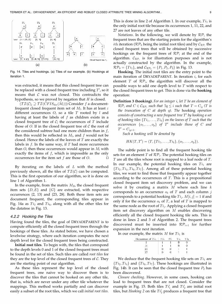
Closure checking. However, in some cases, hooking canlead to frequent trees that are not closed. Consider theexample in Fig. 15. Both tiles Ti01 and Ti02 are initial roottiles, but Hooking 2 on tile Ti02 produces a frequent tree that


Fig. 14. Tiles and hookings. (a) Tiles of our example. (b) Hookings at

iteration 1.

is included in the frequent tree produced by Hooking 1 ontile Ti01, thus being unclosed.

Such cases can be detected quickly by analyzing thehookings already made in the previous iterations. For thispurpose, the hookings performed so far are stored in adatabase denoted by HookingBase. Each hooking isrepresented by a triplet

ðroot frequent tree; hooking tiles; occurrencesÞ;

where root frequent tree is the root attribute tree of thehooking, hooking tiles are the t i les hooking onroot frequent tree for this hooking, and occurrences arethe occurrences of root frequent tree considered in thishooking. As shown in lines 4-12 of Algorithm 2, when anew hooking is proposed, the function Hookings checksthat this new hooking satisfies the closure property withrespect to the hookings of the database. Two nonclosurecases can arise: 1) the new hooking is included into anexisting hooking, and then, the new hooking is discarded(line 5), and 2) the new hooking includes an existinghooking and, then, the existing hooking and the corre-sponding closed frequent tree are erased from the database,and a new closed frequent tree is created from the newhooking, which is registered into the hooking database(lines 8-9).

Preparing the next iteration. In the first iteration, the

seeds of the closed frequent trees to be discovered are the

initial root tiles, grouped into RP0. The frequent trees

grown by hooking tiles on these root tiles are inserted into

RP1 and will be used as the seed for the next iteration

(line 10 of Algorithm 1). However, this is not enough to

discover all of the closed frequent trees of C. We have seen

before that only a fraction of all the root tiles could be

discovered at the beginning of the algorithm; these were the

initial root tiles. The problem is that a tile T can both be the

root tile of a closed frequent tree P and a nonroot tile of

another closed frequent tree P 0. Therefore, for the mappings

of T corresponding to P 0, T will be hooked on other tiles,

preventing it from satisfying the same conditions as the

initial root tiles. In the example, Ti4 is both a subtree in P1

and the root tile of P4. The problem is that if we look at the

mappings of Ti4, this tile does not hook on any other tile,

only for the mapping rooted at occurrence 35: Its “root”

status does not appear frequent with so few information.

Therefore, for all these root tiles that are not initial root tiles,

their discovery is delayed to later iterations, at a moment

where we will have enough information to determine if this

tile was only the subtree of one or more closed frequent

trees or if it can also be the root tile of some other closed

frequent trees. Therefore, after our hooking step, we have to

analyze the hooked tiles to see if they belong to the category

of tiles that will always be hooked somewhere or if they can

become root tiles at the next iteration. This is done in the

DetectNewRootTiles function (Algorithm 3). In line 2 of

Algorithm 3, the tiles T that have been hooked on other tiles

in the current iteration (and so appear in HookingBasei) are

iterated over. In line 3, these tiles T are tested: the left part

of the AND checks that there does not exist any unknown

hooking between these tiles and a given tile T 0; this is done

for all the occurrences of T . If this left part is true, then we

are assured to know everything about the hookings of T .

Here comes the “root” part verification: In the right part of

the AND, we check that there exists at least one occurrence

of T where T does not hook on any other tile. If this part is

also true, then T can be not only a subtree of other closed

frequent trees but also a root tile. This is recorded in line 4.

In our example, Ti4 is one of these candidates to be a root

tile, it has been hooked on Ti1 for occurrences 7 and 19.

There are no other tiles where it can hook (left part of the

AND of line 3 satisfied), and for occurrence 35, it does not

hook on any other tile (right part of the AND also satisfied).

Therefore, Ti4 becomes a new root tile; this will allow the

discovery of closed frequent tree Pi4 in the next iteration.

Algorithm 3. The DetectNewRootTiles function

Input: Set of tiles T IðCÞ, hooking database HookingBase

where HookingBasej are the hookings performed in

iteration j

Output: Tiles of T IðCÞ that have become root

1: Result ;2: for all T 2 T IðCÞ st T 2 HT where

ð; HT; Þ 2 HookingBasei do

3: if [8o 2 LoccðT;DTDÞ 6 9T 0 st T can hook on T 0 and

ððT 0; f. . . ; T ; . . .g; Þ 62 HookingBaseÞ] AND

[9o 2 LoccðT;DTDÞ st T cannot hook on any other

tile for o] then


Fig. 15. Example of the generation of an unclosed frequent tree.

4: Result Result [ T5: end if

6: end for

7: Return Result

4.3 Soundness and Completeness

Theorem 1. The algorithm DRYADEPARENT is sound and

complete, that is, CDryade ¼ C.Proof. Completeness. Let P 2 C be a closed frequent tree. We

want to prove that P is found by DRYADEPARENT. Let

us prove by induction on the depth levels of P that for

every depth level d, Pjd is found at some iteration of

DRYADEPARENT.

For depth level 1, Pj1 is by definition a closed frequent

tree of depth 1, that is, a tile. Therefore, it is found in the

first step of DRYADEPARENT.

For depth level d, let us suppose that the induction

property is true, that is, that there exists an iteration i of

DRYADEPARENT where Pjd is found as an element of

RPiþ1. Let us show that Pjdþ1 is found in a later iterationof DRYADEPARENT.

By the definition of the tiles, all the tiles correspond-

ing to the direct subtrees of Pjd in P have been found in

the first step of DRYADEPARENT, so all these tiles appear

as columns of M in the Hookings procedure. Let S

denote this set of tiles. Because P occurs in at least

" documents, P has at least " occurrences, so the closed

frequent item set algorithm in the Hookings finds a set oftiles f , where at least f S. Let us show that we cannot

have f � S. Suppose that f has one more tile T than S for

the same occurrences. This means that T can also be

hooked on Pjd with the other tiles of S, with occurrences

that include the occurrences of P . Therefore, for all the

mappings of P , new P þ T mappings can be found. This

contradicts the fact that P is closed. Hence, f ¼ S.

We must now show that the test on line 5 of theHookings function (Algorithm 2) is evaluated to true,

that is, that there are no hookings in the hooking base

that includes the hooking of the tiles of f on Pjd (else, no

frequent trees would be built from the hookings of f). In

the same way as we did previously, it is easy to show by

negation that if there was such a hooking, then P would

not be closed.

Hence, the closed frequent tree Pjdþ1, resulting fromthe hookings of the tiles of f on Pjd, is correctly

constructed.

It is inserted intoRPiþ2; hence, the induction property

holds.Therefore, DRYADEPARENT is complete.

Soundness. Let P be a frequent tree outputted by

DRYADEPARENT. We want to show that we have P 2 C,that is, P is frequent, and P is closed with respect to the

set of all frequent trees.Frequency. Suppose by negation that P is not

frequent. It means that either a tile of P is not frequent

or that there exists a depth level of P where the set of

tiles for this depth is not frequent. In both cases, it means

that the closed frequent item set algorithm gave a

nonfrequent result. It contradicts the soundness of

closed frequent itemset algorithm. Hence, P is frequent.

Closedness. Suppose by negation that P is not closed,

that is, there exists a closed frequent tree P 0 in which P is

included for all its occurrences. We consider all the

possible inclusion cases, as shown in Fig. 16:

1. One more sibling node. This case would mean that

the corresponding tile was not closed and, hence,

that the closed frequent item set gave a nonclosed

result. Once again, it contradicts the soundness of

the closed frequent item set mining algorithm.2. One more leaf child node. This case would mean

that a tile hooking has not been discovered or not

been done. Because all the tiles are correctly

found thanks to Lemma 1 and the filling of the

hooking discovery matrix is trivial, it would mean

that either the closed frequent item set algorithm

was not complete, which contradicts the comple-

teness of closed frequent itemset algorithm, or

the hooking was found but later dismissed. Such

a dismissal could only be done by the closure

checking mechanism and only if there is a bigger

hooking for the same occurrences at the same

place. This would mean that P 0 itself is unclosed,

which contradicts the hypothesis.3. One more root parent node. Let T be the root tile of

P as found by DRYADEPARENT. In this case, the

root tile of P 0 (containing P ) is a tile T 0 6¼ T , and T

hooks on T 0. Suppose that there is such a tile T 0.

By definition, it cannot be an initial root tile (or

DRYADEPARENT would have found it), and

neither can it be T (because it hooks on T 0).

Because it was never considered as a root tile, the

hookings of T on T 0 have not been found and donot appear in the hooking database. Therefore,

the condition on line 3 of DetectNewRootTiles

cannot be satisfied for all the occurrences of T ,

and so, T cannot be detected as a root tile.By the definition of the root tile detection

procedure, this case cannot occur.

Hence, P is closed, and we can conclude that thealgorithm DRYADEPARENT is sound. tu

4.4 Complexity

We estimate the time complexity of the DRYADEPARENT

algorithm according to the following parameters:


Fig. 16. Three possible inclusion cases.

. kDTDk, the number of nodes of the input database,

. jCj, the number of closed frequent trees to find,

. d, the average depth of a closed frequent tree of C,and

. jT IðCÞj, the total number of tiles in the closedfrequent trees of C.

Computation of tiles. The tiles are computed with the

LCM2 algorithm [18], whose time complexity is linear with

the number of closed frequent item sets to find. Therefore,

the time complexity of the tile computation step is linear

with the number of tiles:

ComplexityðTile computationÞ ’ OðjT IðCÞjÞ:

Computing the initial root tiles. To determine which tile

is an initial root tile, all the occurrences of all the tiles are

checked. This simple step hence has a time complexity of

ComplexityðInitial root tilesÞ ’ OðkDTDk:jT IðCÞjÞ:

Main iteration. The first step of the main iteration is a

loop repeated as many times as there are elements in RPi.These elements are truncations of closed frequent trees of C,so we have jRPij ¼ �:jCj, where � is a constant:

. “if” of line 7. Determining if there are hookings onan element, RT 2 RPi comes to check all of itsoccurrences; the time complexity is

ComplexityðCheck if hookingsÞ ’ OðkDTDkÞ:

. Hookings procedure. Building the transaction matrixand running the LCM2 algorithm has a timecomplexity of OðkDTDk:jT IðCÞjÞ. The hooking basemust then be checked; the time complexity of thissearch operation is linear with the number ofhookings. An upper bound for the number ofhookings is the number of tiles. Hence,

ComplexityðHookingsÞ ’ OðkDTDk:jT IðCÞjþ jT IðCÞjÞ’ OðkDTDk:jT IðCÞjÞ:

The overall time complexity of the for loop is then

Complexityðfor loopÞ ’ OðjCj � ðkDTDk þ kDTDk:jT IðCÞjÞÞ’ OðjCj:kDTDk:jT IðCÞjÞ:

Then, we have to compute the complexity of the

DetectNewRootTiles procedure. For each tile, there is a

search in the hooking base on line 2 and, then, on line 3,

there is a search on all the occurrences of the tile, which

needs another search in the hooking base. This gives an

overall complexity of

ComplexityðDetectNewRootTilesÞ ’ OðjT IðCÞj:jT IðCÞj:kDTDk:jT IðCÞjÞ

’ OðkDTDk:jT IðCÞj3Þ:

The main iteration is repeated �:d times (with � as a

constant), so its time complexity is

ComplexityðIterationsÞ ’ d:ðComplexityðfor loopÞþ ComplexityðDetectNewRootTilesÞÞ

’ Oðd:ðjCj:kDTDk:jT IðCÞj þ kDTDk:jT IðCÞj3ÞÞ

’ Oðd:kDTDk:jT IðCÞj:ðjT IðCÞj2 þ jCjÞÞ:

The overall time complexity of the whole DRYADEPAR-

ENT algorithm is then

ComplexityðDryadeParentÞ ’ ComplexityðTile computationÞþ ComplexityðInitial root tilesÞþ ComplexityðIterationsÞ

’ OðjT IðCÞj þ kDTDk:jT IðCÞjþ d:kDTDk:jT IðCÞj:ðjT IðCÞj2

þ jCjÞÞ’ OðjT IðCÞj:ð1þ kDTDk þ d:kDTDk:ðjT IðCÞj2 þ jCjÞÞÞ

’ OðjT IðCÞj:d:kDTDk:ðjT IðCÞj2

þ jCjÞÞ:

We have given our complexity formula in terms of the

number of tiles jT IðCÞj. This number of tiles can be

approximated by the number of internal nodes in the

closed frequent trees. With this, we can reformulate the

complexity in terms of kCk, the number of nodes in the

closed frequent trees, and b, the average branching factor of

the closed frequent trees of C. Let INðCÞ be the internal

nodes of the closed frequent trees of C. We have

b ¼ number of edges in Cnumber of internal nodes in C :

The number of edges in a single tree T with N nodes is

N � 1, we deduce that for the set of trees C

b ¼ kCk � jCjkINðCÞk :

Therefore,

kINðCÞk ¼ kCk � jCjb

:

Hence,

jT IðCÞj ’ kINðCÞk ¼ kCk � jCjb

:

The complexity formula can now be written as

ComplexityðDryadeParentÞ ’ O kCk � jCjb

:d:kDTDk:�

ðkCk � jCjÞ2

b2þ jCj

!!:

From the above formulas, we can conclude that the

complexity of DRYADEPARENT is polynomial in the


number of tiles, polynomial on the number of nodes in theclosed frequent trees, inversely proportional to the squareof the average branching factor, linear with the size of thedata, and linear with the average depth of the closedfrequent trees. Such characteristics should allow good scale-up properties; this will be investigated in the next section.

5 EXPERIMENTS

This section reports on the experimental validation ofDRYADEPARENT on artificial and real-world data sets, aswell as an application example on real XML data. TheDRYADEPARENT algorithm will be compared with thestate-of-the-art closed tree mining algorithm, CMTreeMiner[13], using the original C++ implementation of its authors.All runtimes are measured on a 2.8-GHz Intel Xeonprocessor with 2 Gbytes of memory (Rocks 3.3.0 Linux).DRYADEPARENT is written in C++, involving the closedfrequent item set algorithm LCM2 [18], kindly provided byTakeaki Uno. The reported results are wall-clock runtimes,including data loading and preprocessing.

5.1 Artificial Data Sets

In the usual tree mining algorithms studies, at most, thelength (that is, the number of nodes) of the found closedfrequent trees is reported, without any information aboutthe structure of these closed frequent trees. However, thebranching factor and the depth of the closed frequent treesintervene directly in the candidate generation process, so

they are likely to play a major role with respect to thecomputation time. To ascertain this hypothesis, we wrote arandom tree generator that can generate trees with a givennode number N and a given average branching factor b.Nodes are labeled with their preorder identifier, so there areno couples of nodes with the same label in a tree. Wegenerated trees with N ¼ 100 nodes and b 2 ½1:0; 5:0�, bincreasing by an increment of 0.1. For each value of b,10,000 trees were generated. Let T be such a tree. For eachT , a data set DT was generated, consisting simply of200 identical copies of T (we perform this 200-timeduplication of each T to increase the processing time forDT and so reduce the error rate on time measurement).Each DT was processed by both algorithms, with a supportthreshold of 200 (hence, the closed frequent tree to find isthe tree T ), and the processing time was recorded.Eventually, for each value of b, we regrouped the trees bytheir depth d and got a point ðb; dÞ by averaging theprocessing times for all the trees of the average branchingfactor b and depth d. Fig. 17a shows the logarithms of theseaveraged time values with respect to the average branchingfactor b, and Fig. 17b shows the logarithms of theseaveraged time values with respect to the depth d.

Fig. 17a shows that DRYADEPARENT is orders ofmagnitude faster than CMTreeMiner as long as thebranching factor exceeds 1.3, which is the case in most ofthe experiments’ space. For lower branching factor values,CMTreeMiner has a small advantage. Closed frequent treeswith such a low branching factor necessarily have a highdepth, this is confirmed in Fig. 17b. This figure shows thatDRYADEPARENT exhibits a linear dependency on the depthof the closed frequent trees. This is not surprising: eachiteration of DRYADEPARENT computes one more depthlevel of the closed frequent trees, so very deep closedfrequent trees will need more iterations.

CMTreeMiner, on the other hand, shows a dependencyon the average branching factor, but for a given value of b,the computation time varies greatly, being especially highfor low depth values. Because of the constraints on therandom tree generator, a tree that has a low depth with ahigh average branching factor will necessarily have somenodes with a very large branching factor. We plotted inFig. 18 a new curve, showing the computation time withrespect to the maximal branching factor.


Fig. 17. Random trees with 100 nodes. (a) Log(time)/average branching

factor. (b) Log(time)/depth.

Fig. 18. Random trees with 100 nodes, log(time) with respect to the

maximal branching factor.

DRYADEPARENT is nearly unaffected by the maximal

branching factor, but the computation time of CMTreeMi-ner depends strongly on this parameter. In order to

understand how much the behavior of CMTreeMiner and

DRYADEPARENT differ, we analyze below the reasons ofthe dependency to the branching factor of CMTreeMiner

and of the variability of its performances in general.We give a brief reminder of the candidate enumeration

technique of CMTreeMiner, the rightmost branch expan-

sion. To generate candidates with k nodes from a frequenttree with k� 1 nodes, CMTreeMiner tries to add a new edge

connecting to a node of known frequent label and starting at

a node of the rightmost branch of the k� 1 node tree. Allthe nodes of the rightmost branch are explored successively

in a top-down fashion, from the root to the rightmost leaf.

1. Branching factor leads CMTreeMiner to generatemore unclosed candidates by backtracking. For anode with a high branching factor, finding correctlythe set of its frequent children is a classical frequentitem set mining problem, and the highly combina-torial nature of this problem often leads to thegeneration of useless candidates. CMTreeMiner is noexception to this rule: its top-down rightmost branchexpansion technique finds very quickly all thechildren of a node but then needs to systematicallybacktrack to check for frequent subsets of thesechildren. In most cases, this leads to the generationof nonclosed candidates. For example, compare thetwo closed frequent trees in Fig. 19. The linear treeP1 is found without generating any unclosedcandidates. However, the flat tree P2 is found afterthe generation of three unclosed candidates, soaccording to our experiments finding P2 needs7 percent more time than finding P1 in this simplesetting with four nodes and 100 percent more time ina similar setting with 11 nodes.

DRYADEPARENT also has to confront such acombinatorial problem in high-branching-factorcases, but it does so by using the LCM2 closedfrequent item set mining algorithm, which provides,

as of now, the most efficient way to explore thesearch space of closed frequent item sets. Further-more, by discovering the tiles once and for all at thebeginning of the algorithm, DRYADEPARENT avoidsto repeat these complex computations if the same tileappears more than once in the closed frequent trees.

In this problem, CMTreeMiner could probably beimproved by modifying its enumeration techniquein order to use LCM2 for sibling enumeration. Sucha modified algorithm should be similar to the recentCLOTT algorithm by Arimura and Uno, which is anextension of the LCM2 principles to the closedattribute tree case.

2. Candidate generation asymmetry. The previousproblem explains partly why CMTreeMiner isslower than DRYADEPARENT in most cases. As wehave seen, this problem can theoretically be over-come. However, another problem remains, thatcannot be overcome easily, and this problem isessential to the superior performances of ourhooking strategy over any algorithm based onrightmost branch expansion.

Consider the simple closed frequent tree in Fig. 20.As it can be seen, during candidate enumeration,unwanted candidates are generated, because therightmost leaf expansion technique has to test“blindly” all the potential expansions on the right-most branch but can only grow good candidates forcertain expansions. For example, the candidate C2

contains correct information: it corresponds to thefirst level of the closed frequent tree to find.However, as some expansions must be made on thenode labeled B, which is not on the rightmost branchof C2, C2 is eliminated. In the same way, C4 iscomputed for nothing. The children with label C ofthe root node will have to be recomputed incandidate C6, even if it could have been discoveredmuch earlier.

This behavior is not only suboptimal, it alsoundermines the robustness of CMTreeMiner. Con-sider the two closed frequent trees in Fig. 21. Exceptfor the names of the labels, both these closedfrequent trees exhibit the same tree structure, so itis expected that they are discovered in exactly the


Fig. 19. CMTreeMiner candidate enumeration for a linear tree and for a

flat tree.

Fig. 20. CMTreeMiner enumeration for a left-balanced closed frequent

tree.

same amount of time. However, assuming that thesibling processing order is the ascending order oflabels (this is the case in the actual implementationof CMTreeMiner), closed frequent tree R, which isright-balanced, is the ideal case for enumeration byrightmost tree expansion. CMTreeMiner will check43 candidates to discover it. On the other hand, theleft-balanced closed frequent tree L is the worst case,and CMTreeMiner will require to check 79 candi-dates for its discovery. The computation times reflectthis difference in candidate checking: the time forfinding L is 50 percent higher than the time forfinding R, as shown in Table 1.

On the other hand, thanks to its tree-orientationneutral hooking technique, DRYADEPARENT re-quires exactly the same amount of time for proces-sing these two closed frequent trees. For both L andR, DRYADEPARENT will generate three candidates:1) the initial tile with root A, 2) a candidategenerated by the hooking of a tile on respectivelyB or E, and 3) the closed frequent tree L or R by thehooking of another tile on, respectively, F or I.

Last, we compared the scalability of DRYADEPARENT

and CMTreeMiner in both time and space in Fig. 22. Thedata set consists of 1,000 to 10,000 copies of a unique perfectbinary tree of depth 5. We can see that in both time andspace, DRYADEPARENT scales linearly. The memory usageis higher for DRYADEPARENT, but here, the reason ismostly implementation specific: for example, the DRYADE-

PARENT integer type is “integer,” whereas CMTreeMiner’sone is “short,” which is four times smaller on our 64-bitmachine. Moreover, DRYADEPARENT’s internal representa-tion for trees is based on trees of pointers, which uses themost memory, especially on a machine where the pointersare 8 bytes long.

Complexity issues. Here, we evaluate the validity of ourcomplexity analysis in Section 4 when compared to theactual results for the artificial data set.

Fig. 23 compares the logarithm of the processing time forthe real algorithm with the logarithm of the complexityformula in Section 4 with respect to 1) the number of tilesand 2) the average branching factor (the linear behavior ofthe algorithm with respect to the depth has already beenascertained in Fig. 17b). For a given number of tiles

(Fig. 23a) or average branching factor (Fig. 23b), there areseveral trees with different shapes satisfying this constraint,leading to different processing times or estimates. Theshaded area in the figures represents all of these processingtimes (for the real algorithm) or estimates (for the complex-ity estimate).

In Fig. 23a, the estimated curve and the real times matchwell for more than 50 tiles, but for a lesser number of tiles,the real-time curve presents a gentler slope than thecomplexity estimate. For a high number of tiles, DRYADE-

PARENT spends most of its time on hooking tiles, with a lotof iterations. The start-up time needed for loading the dataand creating all the needed data structures is negligiblecompared to the total time in these cases. However, forlower numbers of tiles, there are fewer iterations, andDRYADEPARENT is very fast at completing them. Therefore,the start-up time is no longer negligible compared to thetotal times in such cases. Such start-up processings are nottaken into account in the complexity formula; hence, thedifference occurs between the two curves.

The same behavior can be observed in Fig. 23b, for a highbranching factor cases the real algorithm performs fewerhookings and hence is limited by the start-up time, which isnot reflected in the complexity estimate.

One can also note a visible discontinuity on the curvesfor the complexity estimate. This discontinuity reflects thebehavior of our artificial data generator. For averagebranching factors above 1.9, the generator is allowed toproduce nodes with a very high branching factor, whereasit is not possible for branching factors below it. This allowsthe efficient generation of artificial trees satisfying the givenconstraints, at the price of smoothness. The curves for


Fig. 21. L: left-balanced closed frequent tree. R: right-balanced closed

frequent tree.

TABLE 1Computation Time for Finding Closed Frequent Trees R and L

Fig. 22. Scalability tests on binary trees (time-memory).

DRYADEPARENT also present this discontinuity, although it

is less visible.In conclusion, the complexity estimates that we provided

seem to capture well the behavior of the DRYADEPARENT

algorithm, especially when the algorithm has enough

hooking work to do.

5.2 Real Data Sets

In the tree mining literature, two real-world data sets are

widely used for testing: the NASA data set sampled by Chi

et al. from multicast communications during a shuttle

launch event [25] and the CSLOGS data set consisting of

Web logs collected over one month at the Computer Science

Department of Rensselaer Institute [19].The runtimes obtained for various frequency thresholds

for both DRYADEPARENT and CMTreeMiner are displayed

in Fig. 24.DRYADEPARENT is more than twice faster than CMTree-

Miner on the CSLOGS data set. For the NASA data set, the

performances are similar for high and medium support

values, DRYADEPARENT having a distinct advantage for

the lowest support values. Note that we obtained similar

results with simplified CSLOGS and NASA data sets

consisting only of attribute trees. We were interested to

know why DRYADEPARENT and CMTreeMiner have a

bigger performance difference on the CSLOGS data set than

on the NASA data set. Analyzing the structure of the

computed closed frequent trees in both cases, we found that

in the CSLOGS data set, for the support value 0.003 (lowest

value tested), there are 924 closed frequent trees, with three

nodes on the average, and an average branching factor of

1.6. For the NASA data set, the picture is different: at the

support value 0.1, there are 737 closed frequent trees, with

42 nodes on the average, an average depth of 12, and anaverage branching factor of 1.2.

Discussion. Our artificial experiments have shown thatthe structure of the closed frequent trees to find, especiallytheir branching factor, is a crucial performance factor. Theclosed tree mining algorithm CMTreeMiner, based oncandidate enumeration by rightmost branch expansion,has performances that vary considerably with the branching


Fig. 23. Comparing real processing time and estimated complexity. (a) Log(time)/number of tiles. (b) Log(time)/average branching factor.

Fig. 24. Runtime with respect to support for the NASA/Multicast and

CSLOGS data sets.

factor of the closed frequent trees and even with their

balance. The fact that CMTreeMiner and DRYADEPARENT

have similar performances on the NASA data set, with

closed frequent trees having a quite low branching factor,

and that CMTreeMiner is slower than DRYADEPARENT on

the CSLOGS data set, with closed frequent trees having a

higher branch factor, is consistent with our experiments on

artificial data.Experiments have shown that the new method for

finding closed frequent attribute trees of our DRYADEPAR-

ENT algorithm is not only computation-time efficient but

also robust with respect to the tree structure, delivering

good performances with most tree structure configurations.

Such robustness is a desirable feature for most applications,

especially the applications that deal with trees having a

great diversity of structure, for which the typical structure

of closed frequent trees cannot be predicted.

5.3 XML Application Example

In this last series of experiments, we show the analysis of a

corpus of real XML data. This corpus comes from the XML

Mining Challenge, compiled by Denoyer [26]. We used the

“Movie” corpus, initially designed for a mapping task. The

training part of this corpus has the advantage to contain

well-formed XML documents with meaningful tags, each

document describing one movie.Preprocessing. We preprocessed this corpus in the

following way:

. To all leaf tags corresponded a PCDATA stringgiving the value associated to this tag (for example, atag “name” could have as its associated PCDATA“John Wayne”). All the PCDATA of these tags wereprocessed to get rid of punctuation signs andconvert the text into lowercases. In case of stringswith spaces, like in “John Wayne,” the spaces werereplaced by underscores, with a prefixing under-score, like in “_john_wayne” (so that the Perl parserwe used could handle numeral strings like “_1941”).These normalized strings were used as labels of newnodes added as children of the labeled nodes thatthe original strings were values of.

. We made minor alterations to the structure in orderto convert the original trees to attribute trees. Forthis, tags that represented list items were replacedwith their children, that is, by their actual content.For example, each actor in a movie was representedby a tag named “entry” under a main “cast” tag, andinside this “entry” tag were a “name” and one ormore “roles” tags. We suppressed these intermedi-ary tags and instead created a new tag with theactual name of the actor, which became a child of the“cast” tag. The roles of this actor became children ofthe tag bearing the name of the actor.

. There are two tags, “synopsis” and “review,” whosedata is a short text respectively describing the movieand reviewing it. Each text was cut into words; thestopwords like “the,” “and,” etc., were suppressedfrom this list of words. For each word, only one of itsoccurrences was kept, and all the remaining words

became new tags added as leaves of the “synopsis”and “review” tags.

Performances. In the first experiment, we preprocessed100 documents out of the 693 from the collection and fedthem as input to DRYADEPARENT and CMTreeMiner inorder to analyze the computation time performances. Theresults are given in Fig. 25a, with the average branchingfactor of the closed frequent trees given in Fig. 25b. Thereare no results under a support value of 40 percent, as in thiscase, DRYADEPARENT saturated the memory.

The closed frequent trees have a high branching factor:as expected from the previous experiments, for highsupport values, DRYADEPARENT largely outperformsCMTreeMiner. Surprisingly, for lower support values, thecontrary happens. To understand why this was happening,we analyzed carefully the time spent by DRYADEPARENT inits various tasks. We found that for a support value of40 percent, it was spending 74 percent of its computationtime making closure tests (which corresponds to line 5 ofAlgorithm 2). The problem is that, as we stated in theintroduction, DRYADEPARENT has been designed withheterogeneous data sets in mind, that is, data from variousorganizations about the same topics. Because of the verynature of such data sets, they are currently very difficult tofind. The publicly available data sets, like the one we usehere, usually come from the same organization and so arevery homogeneous. The consequence is that a lot of closedfrequent trees are nearly identical, and so, a lot of hookingsalso resemble each other, with subtle differences. Ourclosure test has been written in a rather naive way: it firstlooks for exact hooking matches in the database and thenfor bigger (the current hooking is included in a bigger


Fig. 25. Comparative results for DRYADEPARENT and CMTreeMiner with

the XMLMovie data set. (a) Computation time. (b) Average closed

frequent tree branching factor.

hooking of the database) and smaller matches (the current

hooking includes a smaller hooking of the database),

iterating on all the possible cases of bigger/smaller

matches. Usually, this is very fast because there are not

that many cases to examine, but with a very homogeneous

data set such as XMLMovie, it became a bottleneck. On the

other hand, the edge-adding strategy of CMTreeMiner

performs better here: the fact that all the closed frequent

trees resemble each other means that it has fewer

candidates to expand, so what is a bad case for DRYADE-

PARENT is a good case for CMTreeMiner.To evaluate the behavior of both algorithms on more

heterogeneous data, we derived a new data set from

XMLMovie. The XMLMovie documents are all rooted with

the “movie” tag. We divided our 100 documents into

10 groups fG1; . . . ; G10g, chose 10 arbitrary tags ft1; . . . ; t10g,

and, in each group Gi, for all the documents of this group,made the tag ti replace the tag “movie” at the root of thetree so that for all i 2 ½1; 10�, the documents in Gi are rootedby tag ti. The new data set, called XMLMovieHtr, is muchmore heterogeneous: all documents are on the same topicand share common tags; however, the small difference inthe roots avoids homogeneity and gives more importance tothe closed frequent trees not using this root.

The performances for the processing of XMLMovieHtrare shown in Fig. 26a, with the average branching factor ofthe closed frequent trees shown in Fig. 26b.

This time, both algorithms could correctly process thedata for all support values. The computation time differencewas important between DRYADEPARENT and CMTreeMi-ner, so we had to use a logarithmic scale for the time inFig. 26a. For all support values, even if the closed frequenttrees to find were complex and numerous (more than 20,000at support ¼ 2 percent), DRYADEPARENT could achieve aseveral-order-of-magnitude improvement over CMTreeMi-ner, processing the data in 45 seconds for a support of2 percent, whereas CMTreeMiner needed 2,846 seconds.Therefore, as expected, DRYADEPARENT is far betteradapted for heterogeneous data than CMTreeMiner.

Closed frequent trees analysis. We now show how theclosed frequent trees found could be useful in an XML datamining application. Our first interest, in such homogeneousdata, is to find a schema common to all of the documentsanalyzed, which could stand for a very basic DTD (theDocument Type Definition, or DTD, is the “grammar” of anXML document. More resources about XML can be found in[27]), especially in cases like XMLMovie where the docu-ments are homogeneous, but no DTD was formally defined.This is close to grammatical inference [28], but the goal ofgrammatical inference on XML data is to find the completeDTD of all the XML documents [29], which is beyond thescope of frequent tree mining. Therefore, we ran DRYADE-

PARENT on XMLMovie with a support of 100 percent; theclosed frequent tree found is shown in Fig. 27. We areassured that all the documents will contain this closedfrequent tree, which can, for example, be useful fordesigning queries on these documents.

With lower support values, the closed frequent trees alsoallow extracting precise information from the data. The nextclosed frequent trees come from the mining of XMLMo-vieHtr with a support value of 5 percent.


Fig. 26. Comparative results for DRYADEPARENT and CMTreeMiner with

the XMLMovieHtr data set. (a) Logarithm of computation time. (b)

Average closed frequent tree branching factor.

Fig. 27. Common schema to all of the 100 documents of XMLMovie.

Following the node nesting, we have the following:

. The information can have a horizontal organization,like in Fig. 28a. Here, the closed frequent tree couldhave been found by a simple frequent item setmining algorithm, it represents the frequent childrenof the “categories” node. We learn that “features”that are in black and white (“bw”) often are availablein a colorized version.

. The information can have a vertical organization,like in Fig. 28b. Here, through the nesting of nodesexpressing data and of nodes expressing what thisdata represents, we can learn that the individual“Cedric Gibbons” was a member of the productionteam of at least five movies and that his job was to bethe art director.

. Finally, most closed frequent trees, like in Fig. 28c,combine vertically and horizontally organized in-formation, which is the major advantage of treemining. Here, we learn that at least 5 percent of themovies are nominated (“_nom” suffix after an awardname) for the following awards: best director for thedirectors’ guild of America and best actor and bestpicture for the Academy awards. This closedfrequent tree can lead to many interpretations, forinstance, that good movies are associated with thecombination of a good director and a good mainactor.

Some closed frequent trees can allow an even fineranalysis of the data. Consider the closed frequent tree inFig. 29, extracted from XMLMovieHtr with a support of2 percent.

This big closed frequent tree is shared by two movies“Rebel without a Cause” (1955) and “The Graduate” (1962).Both of these films are American, were big successes, wonawards, and have a five-star AMG rating. However, moreimportantly, the closed frequent tree was able to capturewell what is common to these movies: they are movies about“coming of age” and “generation gap” (from the keywords),words like “rebellion” and “parents” appear in the synopsis,and words like “generation,” “parents,” “alienation,” and“prosperity” appear in the review. Such words seem tocharacterize well both films made in a prosperous America,but where the young people were less and less attracted bytheir parents’ model and tried to find another way of life.Searching Google with these two film names togetherconfirmed that these two films are grouped together bysociologists when analyzing the America of the 1950s and

1960s (see, for example, [30], available at http://www.lib.berkeley.edu/MRC/nickray.html). The shopping site Ama-zon.com also rates the two movies as similar. Therefore,what is very interesting with that closed frequent tree is thatit could group together two similar movies and even provideelements to describe what make them similar. Such kind ofclosed frequent trees are particularly useful for conceptualclustering, by grouping together similar elements andcharacterizing the cluster. The particular advantage here,due to the structural analysis of XML data, is that it providesvery fine grained information, which could be particularlyuseful to people doing a detailed analysis of the data.

6 CONCLUSION AND PERSPECTIVES

In this paper, we have presented the DRYADEPARENTalgorithm, based on the computation of tiles (closedfrequent attribute trees of depth 1) in the data and on anefficient hooking strategy that reconstructs the closedfrequent trees from these tiles. This hooking strategy isradically different from current tree mining approaches likeCMTreeMiner. Whereas CMTreeMiner uses a classicalgenerate-and-test strategy to build candidate trees edge byedge, the hooking strategy of DRYADEPARENT finds acomplete depth level at each iteration and does not needexpensive tree mapping tests.

Thorough experiments have shown that DRYADEPAR-ENT is faster than CMTreeMiner in most settings. Moreover,the performances of DRYADEPARENT are robust withrespect to the structure of the closed frequent trees to find,whereas the performances of CMTreeMiner are biasedtoward trees having most of their edges on their rightmostbranch.

We also have shown that in the analysis of XML data, aslong as the data is heterogeneous, DRYADEPARENT canprovide excellent performances, allowing a near-real-timeanalysis. We also have shown that the closed frequent treesfound could capture very interesting information from thedata.

We have proposed new benchmarks, taking into accountthe structure of the closed frequent trees, to test thebehavior of tree mining algorithms. As far as we know,such kind of tests is new in the tree mining community.

Improving these benchmarks and making more detailedanalyses are some of our future research directions. Wethink that our experiments proved that such tools arevaluable for the tree mining community. We also plan toextend DRYADEPARENT to structures more general thanattribute trees.


Fig. 28. Some closed frequent trees extracted from XMLMovieHtr with a support value of 5 percent. (a) Horizontal closed frequent tree. (b) Vertical

closed frequent tree. (c) Hybrid closed frequent tree.

ACKNOWLEDGMENTS

The authors wish to thank especially Takeaki Uno for theLCM2 implementation and Yun Chi for making availablethe CMTreeMiner implementation and giving us the NASAdata set. This work was partly supported by the grant-in-aid of scientific research No. 16-04734.

REFERENCES

[1] R. Agrawal and R. Srikant, “Mining Sequential Patterns,” Proc.11th Int’l Conf. Data Eng. (ICDE ’95), P.S. Yu and A.S.P. Chen, eds.,pp. 3-14, citeseer.ist.psu.edu/agrawal95mining.html, 1995.

[2] H. Mannila, H. Toivonen, and A.I. Verkamo, “Discovery ofFrequent Episodes in Event Sequences,” Data Mining and Knowl-edge Discovery, vol. 1, no. 3, pp. 259-289, citeseer.ist.psu.edu/mannila97discovery.html, 1997.

[3] T. Asai, K. Abe, S. Kawasoe, H. Arimura, H. Sakamoto, and S.Arikawa, “Efficient Substructure Discovery from Large Semi-Structured Data,” Proc. Second SIAM Int’l Conf. Data Mining (SDM’02), pp. 158-174, Apr. 2002.

[4] A. Inokuchi, T. Washio, and H. Motoda, “Complete Mining ofFrequent Patterns from Graphs: Mining Graph Data,” MachineLearning, vol. 50, no. 3, pp. 321-354, 2003.

[5] M. Kuramochi and G. Karypis, “An Efficient Algorithm forDiscovering Frequent Subgraphs,” IEEE Trans. Knowledge and DataEng., vol. 16, no. 9, pp. 1038-1051, Sept. 2004.

[6] J.-H. Cui, J. Kim, D. Maggiorini, K. Boussetta, and M. Gerla,“Aggregated Multicast—A Comparative Study,” Proc. Second Int’lIFIP-TC6 Networking Conf. (NETWORKING ’02): NetworkingTechnologies, Services, and Protocols; Performance of Computer andComm. Networks; and Mobile and Wireless Comm., pp. 1032-1044,2002.

[7] D. Shasha, J.T.L. Wang, and S. Zhang, “Unordered Tree Miningwith Applications to Phylogeny,” Proc. 20th Int’l Conf. Data Eng.(ICDE ’04), p. 708, 2004.

[8] M.J. Zaki, “Efficiently Mining Frequent Trees in a Forest:Algorithms and Applications,” IEEE Trans. Knowledge and DataEng., vol. 17, no. 8, pp. 1021-1035, Aug. 2005.

[9] L.H. Yang, M.L. Lee, W. Hsu, and S. Acharya, “Mining FrequentQuery Patterns from XML Queries,” Proc. Eighth Int’l Conf.Database Systems for Advanced Applications (DASFAA ’03), p. 355,2003.

[10] M.J. Zaki and C.C. Aggarwal, “XRules: An Effective StructuralClassifier for XML Data,” Proc. ACM SIGKDD ’03, citeseer.ist.psu.edu/zaki03xrules.html, 2003.

[11] A. Termier, M. Rousset, and M. Sebag, “Dryade: A New Approachfor Discovering Closed Frequent Trees in Heterogeneous TreeDatabases,” Proc. Fourth IEEE Int’l Conf. Data Mining (ICDM ’04),pp. 543-546, 2004.

[12] H. Arimura and T. Uno, “An Output-Polynomial Time Algorithmfor Mining Frequent Closed Attribute Trees,” Proc. 15th Int’l Conf.Inductive Logic Programming (ILP ’05), 2005.

[13] Y. Chi, Y. Yang, Y. Xia, and R.R. Muntz, “CMTreeMiner: MiningBoth Closed and Maximal Frequent Subtrees,” Proc. Eighth Pacific-Asia Conf. Knowledge Discovery and Data Mining (PAKDD ’04), 2004.

[14] P. Kilpelainen, “Tree Matching Problems with Applications toStructured Text Databases,” PhD dissertation, Technical Report A-1992-6, Dept. of Computer Science, Univ. of Helsinki, Nov. 1992.

[15] N. Pasquier, Y. Bastide, R. Taouil, and L. Lakhal, “DiscoveringFrequent Closed Itemsets for Association Rules,” Proc. Seventh Int’lConf. Database Theory (ICDT ’99), 1999.

[16] R. Agrawal and R. Srikant, “Fast Algorithms for MiningAssociation Rules,” Proc. 20th Int’l Conf. Very Large Data Bases(VLDB ’94), 1994.


Fig. 29. Biggest closed frequent tree from XMLMovieHtr with a support of 2 percent.

[17] M.J. Zaki and C.-J. Hsiao, “Charm: An Efficient Algorithm forClosed Itemset Mining,” Proc. Second SIAM Int’l Conf. Data Mining(SDM ’02), Apr. 2002.

[18] T. Uno, M. Kiyomi, and H. Arimura, “LCM v.2: Efficient MiningAlgorithms for Frequent/Closed/Maximal Itemsets,” Proc. SecondWorkshop Frequent Itemset Mining Implementations (FIMI ’04), 2004.

[19] M.J. Zaki, “Efficiently Mining Frequent Trees in a Forest,” Proc.Eighth ACM SIGKDD Int’l Conf. Knowledge Discovery and DataMining (KDD ’02), July 2002.

[20] T. Asai, H. Arimura, T. Uno, and S. Nakano, “DiscoveringFrequent Substructures in Large Unordered Trees,” Proc. SixthInt’l Conf. Discovery Science (DS ’03), pp. 47-61, 2003.

[21] S. Nijssen and J.N. Kok, “Efficient Discovery of FrequentUnordered Trees,” Proc. First Int’l Workshop Mining Graphs, Treesand Sequences (MGTS ’03), 2003.

[22] Y. Xiao, J.-F. Yao, Z. Li, and M.H. Dunham, “Efficient Data Miningfor Maximal Frequent Subtrees,” Proc. Third IEEE Int’l Conf. DataMining (ICDM ’03), p. 379, 2003.

[23] M.J. Zaki, “Efficiently Mining Frequent Embedded UnorderedTrees,” Fundamenta Informaticae, special issue on advances inmining graphs, trees and sequences, vol. 65, nos. 1-2, pp. 33-52,Mar./Apr. 2005.

[24] T.H. Cormen, C.E. Leiserson, R.L. Rivest, and C. Stein, “DynamicProgramming,” Introduction to Algorithms, second ed., pp. 323-369,MIT Press, 2001.

[25] R. Chalmers and K. Almeroth, “Modeling the Branching Char-acteristics and Efficiency Gains of Global Multicast Trees,” Proc.IEEE INFOCOM ’01, Apr. 2001.

[26] L. Denoyer, “XML Mining Challenge,” http://xmlmining.lip6.fr/Corpus, 2006.

[27] W. Consortium, Extensible Markup Language (XML) 1.0, fourthed., http://www.w3.org/TR/REC-xml/, 2006.

[28] E. Gold, “Language Identification in the Limit,” Information andControl, vol. 10, pp. 447-474, 1967.

[29] Y. Papakonstantinou and V. Vianu, “DTD Inference for Views ofXML Data,” Proc. ACM SIGMOD, 2000.

[30] I.C. Jarvie, “America’s Sociological Movies,” Arts in Soc., vol. 10,no. 2, pp. 171-181, Summer-Fall 1973.

Alexandre Termier received the PhD degreefrom the University of Paris-South in 2004. He isan assistant professor of computer science atthe University of Grenoble. His research inter-ests include data mining, parallelism, and peer-to-peer networks. For data mining, he is espe-cially interested in mining trees and directedacyclic graphs.

Marie-Christine Rousset is a professor ofcomputer science at the University of Grenoble.Her research interests include knowledge repre-sentation and information integration. In particu-lar, she works on the following topics: logic-based mediation between distributed datasources, query rewriting using views, automaticclassification and clustering of semistructureddata (for example, XML documents), peer topeer data sharing, distributed reasoning. She

has published more than 70 refereed international journal articles andconference papers and participated in several cooperative industry-university projects. She received a best paper award from AAAI in 1996and has been nominated as an ECCAI Fellow in 2005. She has servedin many program committees of international conferences and work-shops and on the editorial boards of several journals.

Michele Sebag received the degree in Mathsfrom Ecole Normale Superieure, Paris, and thePhD degree in computer science in 1990 andher Habilitation in 1997. She has been with theCentre National de la Recherche Scientifique(CNRS) since 1991, where she has been asenior researcher (Directeur de Recherche)since 2003. Primarily grounded in applicationsfor numerical engineering, her research interestsinclude relational learning and inductive logic

programming, ensemble methods, evolutionary computation and genet-ic programming, and statistical learning. She is on the editorial boards ofthe Machine Learning Journal and Genetic Programming and EvolvableHardware. She is an associate editor of Knowledge and InformationSystems and was an associate editor of the IEEE Transactions onEvolutionary Computation from 1997 to 2003.

Kouzou Ohara received the ME degree ininformation and computer sciences and thePhD degree from Osaka University in 1995and 2002, respectively. He is currently anassistant professor in the Institute of Scientificand Industrial Research, Osaka University. Hisresearch interests include machine learning,data mining, and personalization of intelligentsystems. He is a member of the IEEE, the AAAI,the IEICE, the IPSJ, and the JSAI.

Takashi Washio received the PhD degree innuclear engineering from Tohoku University,Japan, in 1983, on the topic of process plantdiagnosis based on qualitative reasoning. He isa professor in the Institute of Scientific andIndustrial Research (ISIR), Osaka University. AtISIR, he works on the study of scientificdiscovery, graph mining, and high-dimensionaldata mining. He received the best paper awardfrom the Atomic Energy Society of Japan in

1996, the best paper award from the Japanese Society for ArtificialIntelligence in 2001, and the Journal Award of Computer AidedChemistry in 2002. He is a member of the IEEE Computer Society.

Hiroshi Motoda received the BS, MS, and PhDdegrees in nuclear engineering from the Uni-versity of Tokyo. He is a professor emeritus atOsaka University and a scientific advisor of theAsian Office of Aerospace Research and Devel-opment, Air Force Office of Scientific Research,US Air Force Research Laboratory (AFOSR/AOARD). His research interests include ma-chine learning, knowledge acquisition, scientificknowledge discovery, and data mining. He is a

member of the steering committee of PAKDD, PRICAI, DS, and ALT. Hereceived the best paper award twice from the Atomic Energy Society ofJapan (in 1977 and 1984) and three times from JSAI (in 1989, 1992, and2001), the outstanding achievement award from JSAI in 2000, and theOkawa Publication Prize from the Okawa Foundation in 2007. He is amember of the IEEE Computer Society.

. For more information on this or any other computing topic,please visit our Digital Library at www.computer.org/publications/dlib.


DryadeParent, An Efficient and Robust Closed Attribute Tree Mining Algorithm

Documents

Transcript of DryadeParent, An Efficient and Robust Closed Attribute Tree Mining Algorithm