An integrated use of 2D and 3D raster modulesfor atmospheric fluxes modeling in GRASS

Marco CIOLLI, Roberto REA, Alfonso VITTI, Dino ZARDI, Paolo ZATELLI

Dipartimento di Ingegneria Civile e Ambientale,Università degli Studi di Trento,

Via Mesiano 77, 38100 Trento, Italy.tel. +39-0461-88-2618, fax +39-0461-88-2672,

e-mail Paolo.Zatelli@ing.unitn.it

Abstract

Numerical simulation of atmospheric phenomena closely depending on interaction with ground re-quires a detailed representation of values of various fields of distributed land variables such as solarirradiance, local slope and exposition, land covering, underground nature and so on. In some cases itis convenient to integrate simple models simulating the phenomena above into a system for manage-ment of geographic information. However, the intrinsic 3D nature of these phenomena has been so faran obstacle to the implementation of suitable models, due to the impossibility of managing such databy means of the available Geographic Information Systems. The modules which have been recentlymade available in GRASS for management and treatment of 3D data allow the development of suitablealgorithms by combination of both 2D and 3D data and modules. In the present work we show somepreliminary results of a simulation of slope winds which develop along sloping valley side-walls dueto ground heating or cooling. Simple classical parameterizations of wind and temperature profiles,obtained in the case of plain tilted slope (Prandtl, 1942; Defant, 1949), have been used along withdistributed data over a 2D domain (incidence radiation, land nature and use, local slope from DTM,etc.) to evaluate a suitable energy balance at ground level and fields of meteorological variables suchas air temperature, pressure and wind velocity in a 3D domain over a surface. In particular two dif-ferent methods have been developed to evaluate the normal vector to the surface and the distance of agiven point from the surface, which are key parameters for the subsequent application of atmosphericmodels. The first method for the evaluation of the line connecting a point P within the valley to theunderlying boundary surface consists in identifying that point over the surface which displays min-imum distance from P. Within a volume divided in discrete cells it is possible to take into accountslope inclination and orientation at cell ground which satisfies the minimum distance condition fromthe cell centered in P. The second method for the identification of the normal to the surface consists individing the volume above the surface in layers, and then using the 3D algebra (r3.mapcalc) to eval-uate the normal, according to the surface shape. Further developments will include an optimizationof parameterization adopted in the model and tests check by compare with both the output of othermodels and field measurements.

1. Introduction

Most of the current Geographic Information Systems (GIS) are able to manage and analyze bidimen-sional data and to visualize them in a thredimensional space. The third dimension is often used asattribute of 2D data and not as a real coordinate: bidimensional maps are simply “spread” over a Dig-ital Elevation Model (DEM) to give the third dimension effect in data visualization. These feature,however, are not enough to correctly describe and handle 3D data and phenomena.

In the GRASS 5 GIS a set of new 3D raster module is now available. These modules allow not onlythe management and the analysis of 3D data but also the development of full models and algorithmsapplied to time-depending phenomena and space varying data and their relationships. Many of these3D phenomena closely depend on the interaction with the ground and the landscape features whichconstitute one of the main field of classic applications of GIS. Therefore the availability of a tool forthe joint use of 2D classical GIS information and of 3D data is fundamental for natural phenomenamodeling.

Models of atmospheric processes occurring close to the ground and GIS display a point of contactsince most of the input variables of lower atmosphere phenomena are distributed on the land surface.In this paper an integrated and complementary use of 2D and 3D GRASS modules is presented. Inparticular, a simple mathematical model to depict the behavior of slope winds has been developedimposing two different sets of boundary conditions to model wind velocity, potential and virtual po-tential temperature and to describe the humidity flux from the ground to the atmosphere. Land coverand variables like local slope, irradiance and exposition have a large influence on the evolution of theslope winds and of the evaporation processes.

Slope winds are air fluxes which develop in the first tens of meters of the atmosphere along aslope. As these fluxes are parallel to the slope, the coordinates used to describe the phenomenonare not horizontal and vertical but parallel and normal to the slope. Prandtl (1942) derived a simplesolution to describe the velocity of the wind along the direction parallel to the ground considering a dryatmosphere. To take in to account water vapor exchange between the ground and the atmosphere theboundary conditions imposed by Prandtl have been modified. The new solution for the wind velocity isnot formally different from the previous but now the atmosphere is considered moist and humidity fluxcan also be evaluated. Wind velocity depends on the slope angle of the ground, on the temperature ofthe air and on the distance from the ground measured along the direction perpendicular to the motion.

A new GRASS 3D module has been written to evaluate the coordinate n of a point in the 3Dvolume measured along the direction normal to the terrain surface. This module can also generatea 3D raster where each cell is assigned the value of the cell on the surface belonging to the samenormal vector. This option allows also the transfer of bidimensional information into the 3D rasterenvironment. The extension of the Prandtl’s solution for the moist air has been completely developedusing the GRASS 3D maps algebra based on the module r3.mapcalc.

2. Slope winds

Slope winds are air flux developed by the cyclical heating and cooling of the land due to the solarradiation. The phenomenon interests the mountain valleys where significant temperature gradientoccur, in particular in the layers of the atmosphere close to the mountain slope. For the general aspectsof the phenomenon we refer to Wagner (1923, 1938) and for the theoretical formulation to Prandtl(1942), as illustrated by Defant (1949).

In figure 1 it is outlined the daily development of the wind circulations in a mountain valley.

Figure 1: Schematic representation of the air flux in a valley during a normal day.

At sunrise the air in the valley is colder than the air out of the valley and this generates an airflux from the valley to the plan called mountain wind. In this moment of the day the slope surfaceincreases its temperature and heats the air at land contact. The heated air, displaying a lower densitycompared to the rest of the atmosphere, begins to move towards upward, along the slope, this air fluxis known as up-slope wind. The cool air coming from the center of the valley replaces the one thatis ascending. The development of the phenomenon the temperature gradient between the valley andthe plan vanishes and the mountain wind stops. Now the slope wind continues to heat the air in thevalley which soon becomes warmer than the air over the plain. This difference originates an air flux,from the plain to the mountain valley, which begins to replace the air in the valley. The afternoon iscoming and solar radiation is decreasing, as consequence the up slope wind slows too and then stops.Now only the air flux going from the plain to the valley is present, it is named valley wind. In the lateafternoon the land has a lower temperature compared to the atmosphere which, in the first meters nearthe ground, begins to cool. Cold air begins to move towards the bottom, along the slope, this air flux isknown as down-slope wind. Again the temperature gradient between the plain and the air valley tendsto zero, a new equilibrium situation develops. In the evening the down slope wind is responsible forthe cooling of the air in the valley which during the night becomes colder than the plan one. The laststep is the new complete development of the mountain wind blowing from the mountain valley to theplain.

2.1 Theoretical formulation

In Prandtl’s work (1942) the mountain slope is outlined with a slanted plan of an angle � with respectto the horizontal and unperturbed atmospheric conditions are stable. In these conditions an elementof air volume, receiving heat from the warm surface, begins to move upwards along the slope. Giventhe system geometry, it is convenient to use a reference frame with the axis of the abscissas � parallelto the slope and the axis of the coordinates � along the normal direction. The flux of sensible heatcoming from the ground is responsible for the temperature increasing of the air mass closest to theground. The air element, heated from the thermal flux, has a lower density with respect to the sur-rounding atmosphere therefore it is subject to one buoyancy that supports the motion. Slope windsdepend on the heat flux going from the soil to the atmosphere so in his theoretical formulation Prandtlassumed the phenomenon dependent on the temperature value. In particular he adopted the potentialtemperature, which is a widely used parameter in physics of the atmosphere. Potential temperature isthe temperature an element of air volume would have if lead to a reference pressure ��� (1000 hPa),along an adiabatic transformation. Absolute temperature � and potential temperature � are tied by theequation: ��� � ����� ���� (1)

where � is the atmospheric pressure, � the gas constant for dry air and ��� is the specific heat atconstant pressure, (Stull, 1997). In Prandtl’s formulation potential temperature is expressed as thesum of a linear function of the � coordinate and an anomaly ��� due to the heat flux from the slopesurface along the � direction. This relation is expressed by the equation:�������� �!�"�#����$%��& (2)

where �'� is the potential temperature vertical gradient in standard atmospheric conditions. In a genericpoint of the volume the air flux velocity (*) , along the direction parallel to the slope, is function ofthe distance from the land, measured along the direction � perpendicular to the slope. Omitting themathematical derivation, the velocity of the slope wind can be expressed as:(+),�-�/. 021!354� � 35687:9<;>=%?A@CBED $%��FHGI& (3)

while the anomaly of potential temperature is:����-� 7 9<;I=%?KJML @ $%��FHGI& (4)

The parameters which appear in these two equations are:� anomaly temperature at the ground level���N$%� & OCP5Q;0 gravity acceleration;

1 � RSUTWVCX R%Y ;354 air thermal diffusivity;3H6 air kinematic viscosity;GZ�\[ ]U^U_+^U`aUbdcIe:fhgji�k>lnm R = ] , typical length scale of the phenomenon;� slope angle.

To determine the value of the � parameter it is necessary to impose a boundary condition to theinterface ground-atmosphere. At the surface level, the conduction of the sensible heat is responsiblefor the temperature increasing of the air mass. Fourier law describes such a mechanism and representsthe boundary condition: o 4 �qp"r 4ts ���s � OuPHQ (5)

where

o 4 is the sensible heat flux and v�w�xv ; is potential temperature variation in the � direction. Thevariation along the � direction can be neglected since the motion is uniform along the slope. Sub-stituting (4), for the anomaly of potential temperature, into (5) we obtain the expression for the �parameter: �/� o 4 Gr 4 (6)

In the following the criteria to evaluate the sensible heat flux as function of land properties, incomingsolar radiation and atmospheric conditions will be explained.

The peculiarities of Prandtl (1942) solution are:y wind velocity vanishes on the soil;y at this boundary the value of ���:z z is imposed (Prandtl imposed directly the value of � ).

To take into account the influence of moisture and evaporation processes on the evolution of themotion, equation (3) can not be used because further hypothesis should be made; so the informationregarding moist air is considered using virtual potential temperature instead of potential temperature.Equations are like those of Prandtl (1942) solution but instead of potential temperature the variablevirtual potential temperature is adopted here. The expressions for the anomaly of virtual potentialtemperature and the wind velocity are:��� z z{ �-| R 7:9 O } |M~:� � � ��| S 7:9 O } �I��� � � (7)(+),� � r��� �I��� � � S�� | R 7:9 O } �I��� � � p�| S 7:9 O } |�~�� � �N� (8)

The hypothesis to obtain the solution for moist air in presence of evaporation are the same of Prandtl(1942) solution with two differences:

y wind velocity is not zero at the soil level;y boundary conditions to obtain | R and | S are imposed in order to take into account the evaporationprocesses.

The first boundary condition is the conservation of heat fluxes at the contact surface between canopyand air (n=0). This surface is not necessary the soil but can be a suitable height (i.e. average canopythickness). So equation (5) has been imposed considering for the sensible heat the following expres-sions: o 4 �qpAr 4�s ��� z z{s � OCP5Q (9)

The second condition imposed is the conservation of humidity flux between canopy surface and atmo-sphere (n=0) associated to the imposed of the Bowen ratio:o�� �����������<� ���� (,� ;>� �H$��C�Zp��+� ;>� ��& (10)� ~A� o 4o�� � p"r�� v�xW� ��v ; � ;>� ���� (,� ;>� �H$��C�Zp��+� ;>� ��& (11)

where ��� is the specific humidity flux from canopy, �¡� is the water vapor bulk transfer coefficient,� � is evaporation’s latent heat, �u� is specific humidity on the vegetation surface, �+� ;>� � and (,� ;I� � areatmosphere’s specific humidity and wind velocity on the surface.So two expression for | R and | S have been obtained:

| R �¢p£$U¤Zp � ��� � ~*¥�¦§ � 6©¨Mª¬« � 9 «u­ OuPHQ¯®° )%± ; l+²r & ³N´¶µ �� � ����¥�¦§ � 6©¨Mª¬« � 9 «u­ OuPHQ¯®° )%± ; l+² k $ ¤·� � ~:& � (12)

| S � ³N´¶µ�¸� � ��� ¥ ¦§ � 6 ¨ ª¹« � 9 «C­ OuPHQ ®° )�± ; l+² k $U¤·� � ~:& � (13)

3. Heat fluxes at the ground level

In the first millimeters of atmosphere, at the ground level, the heat flux depends on both turbulentand molecular transport mechanisms. Molecular transport allows heat transfer from the ground to theatmosphere, while turbulent transport transfers heat inside the atmosphere as outlined in figure 2. Farfrom this first layer heat flux in the atmosphere depends on convective phenomena.

Figure 2: Turbulent, molecular and effective thermal flux component for a day time convective process(Stull 1997).

In this layer we assume that the heat fluxes can be described through the Fourier law for the thermalconduction (5). As outlined in figure 3 it is possible to simply express the heat fluxes budget throughfour different terms as follows.

Figure 3: Heat fluxes for an thin air layer during day time.

p oº) � o 4 � o� p o¼»(14)

where o º) = net radiation flux;o 4 = sensible heat flux;o��= latent heat flux;o»= ground (molecular) heat flux.

and fluxes from ground to the atmosphere are positive. In the day time situation p o º) is positive,sensible heat flux

o 4 and latent heat flux

o�are positive due to thermal conduction and humidity

transport phenomena respectively. Molecular heat flux inside the ground p o�» is positive because theenergy is transfered from the heated surface. In the night time situation p o º) is often negative due tothe long-wave radiation emitted toward the atmosphere (IR),

o 4 is negative,

o¼�is negative due to

dew or frost formation. The heat flux from the warm soil layers to the cold surface p o�» is negativetoo.

3.1 Net radiation

Net radiation flux

o º) can be splitted in four terms:oº) �¾½¿)!À��K½¿)!Á��A¼ÀÃ�A¼Á (15)

where: ½¿)ÄÀ = downwelling transmitted shortwave radiation;½¿)ÄÁ = upwelling reflected shortwave (solar) radiation;¼À = longwave infrared (IR) radiation diffused down;¼Á = longwave IR radiation emitted up.

It is possible to split the net radiation in long and short wave components because the peak in the solarspectrum is at the normal visible light wavelengths, while the system earth-atmosphere emits mainlyat the infrared wavelengths.

This is not exhaustive in describing radiation phenomena, only some useful information to under-stand the phenomena bases are provided.

3.1.1 Short wave radiation

The intensity Å of the solar radiation hitting the more external atmospheric layers is called extrater-restrial solar irradiance or solar constant, its value is between ¤>Æ�Ç ³ and ¤>Æ�È ³ �ÊÉÌË 9 S � . This value ismeasured with respect to a surface normal to the sun beams. The solar irradiance arriving on the earthis a fraction of the extraterrestrial solar irradiance. Gases composing the atmosphere, water vapor andaerosols produce complex physical phenomena as absorption and scattering reducing the irradiancevalue at the land level. Solar constant depends also on the earth orbit around the sun. Also clouds actas a reducing factor. The solar irradiance at ground level can be evaluate through the relation:½Í)�À2�¾Å�Ρ�'� 6 JdL @ � ; (16)

where Å is the solar constant, ÎÏ� is the orbital coefficient, � 6 is the atmospheric transmissivity coef-ficient and � ; is the incidence angle. Incidence angle is the angle between the direction normal to thesurface and the sun beam direction.

A fraction of the solar irradiance hitting the earth surface is absorbed, a fraction is transmitted andanother one is reflected. The reflection coefficient is often called albedo and is defined as:Ð � reflected radiation

incident radiation(17)

Reflected radiation can be evaluated through the relation:½¿)ÄÁK� p Ð ½¿)ÄÀ (18)

3.1.2 Long wave radiation

The long wave radiation term ¼Á in (15) can be evaluated by using Stefan-Boltzmann equation:¼Á2�Ñ:Ò%ÓKÔnÕ�Ö¼� ] (19)

where Ô+Õ�Ö×�/Ø2ÙÊÇÛÚA¤ ³ 9ÝÜ �ÞÉ Ë 9 S ½ 9 ] � is the Stefan-Boltzmann constant and Ñ�Ò�Ó is the infrared emis-sivity. The term of diffusive radiation is more complex and difficult to evaluate. It is possible to splitit in three terms: ¼À2�-ÂM�Uß!��Âd�Uàá��Âd�¯â (20)

where Âd�¯ß is the Rayleigh coefficient for the irradiance fraction scattered by the atmosphere. The termÂM� à is the Ångström coefficient for the fraction diffused by the aerosols and Â5�¯â describes the fractiondiffused by multiple spreads between earth surface and atmosphere (greenhouse effect). A sufficientprecision can be obtained also using the Burridge and Gadd equation (Stull, 1997) giving directly theinfrared net radiation: º �ÂãÀÃ�AÂÁ2�ä$ ³ Ù ³ È�å"���H&¿$U¤¡p ³ Ùæ¤�Ô § _ p ³ Ù¹Æ,Ô §Ûç p ³ Ù¹Ç,Ô §Ûè & (21)

where Ô § is the clouds cover factor and the subscripts é , ê , � stand for high, medium and low levels.The term å is the air density and �,� is the specific heat at constant pressure.

The net radiation flux can then be expressed as follows:o º) � ÅëÎ�� 6 JdL @ � ; �# º day time;�  º night time.(22)

4. Sensible and latent heat

The Monteith formulation for the sensible and latent heat fluxes (Monteith 1975, 1990) has beendeveloped from Penman work where only physical variables are used. Monteith has introduced also aphysiological parameter: the leaves resistance. This term describes the resistance to the water vaporflux from the leaves to atmosphere. Leaves resistance can be outlined as a set of resistances in seriesand in parallel. The leaf resistance can be written as:ìIí � ìIî>ïãì §ì>îIï � ì § � ì âÄ��) (23)

where ì>î>ï is the stomatal resistance, ì § the cuticle resistance and ì5ð the mesophyll one. A section ofa leaf is shown in figure 4.

Figure 4: Leaf resistances to water transfer flux (Bullini, 1995) outline.

In table 1 the values of the resistances for some species vegetables are reported. The term ì � is theaerodynamic resistance to water vapor transfer.

water vapor resistanceñ �·| Ë 9 RUòSpecies ì � ì>îIï ì §Betulla verrucosa 0.80 0.92 83Quercus robur 0.69 6.70 380Acer platanoides 0.69 4.70 85Helianthus annuus 0.55 0.38 –

Table 1: Indicative values for aerodynamics, stomatal and cuticle resistance to water vapor transfer(Bullini, 1995).

The resistance term ¸ â!�W) is smaller than cuticle and stomatal ones and can be neglected. Observing(23) and the table 1, values for leaf resistance can be approximated by the only stomatal resistance:ìIí � ì>îIïãì §ì>îIï � ì § � ì â!�W)áó ìIî>ï (24)

The water flux from leaf to the atmosphere depends mainly on stomatal resistance, water evaporatesinside the mesophyll and water vapor diffuses into the atmosphere when the stomatal pores are openand atmospheric conditions are favorable.

The Monteith equations for sensible and latent heat fluxes are:o 4 � ì 4 �Iô�ôÃ$Up o º) � o¼» & �#åA��� � �d)d$%�Û&�põ��$%�Û& �ì 4 �Iô�ôö� � $ ì � � ì>î>ï & (25)o� � � $ ì � � ì>îIï &¿$¯p o º) � o» & �#å"��� � �I)M$��Û&�põ�N$��Û& �ì 4 �Iô�ô*� � $ ì � � ìIî>ï & (26)

where ì 4 is the aerodynamic resistance to sensible heat transfer and �:ô�ô is the specific humidity varia-tion with the temperature in saturation conditions while � is the psychrometric constant.

4.1 Ground heat flux

Ground heat flux can be obtained from molecular heat conduction law and from the second law ofthermodynamics. Using the force-restore method (Stull, 1997) the soil can be outlined with two layers.The superficial layer is affected by the daily thermal variation while the deeper one displays a constanttemperature. The depth of the first layer can be evaluated from the complete solution of the soilconduction equation. Only the equation for the ground heat molecular flux is reported:o» �qp"� »�÷ ) s �

»s�ø � �5ù � »ú÷ )û ÷ )*$�� ð p�� » & (27)

where � » is the soil thermal capacity, � » s the first layer temperature which changes with the time,� ð is the deep layer temperature and diffusiveû

is the period of thermal cycle inside the first soil layer.A numerical time wise solution of the above equation can be obtained starting from a known initialcondition.

4.2 Simple parameterization

A parameterization of the sensible and latent heat fluxes at ground level simpler than the above onesadopts the Bowen ratio coefficient: � ~�� o 4o�� (28)

Ground heat flux can be outlined as a fraction of the incidence net radiation flux:o¼» ��ü o¼º) (29)

where ü � ³ Ùæ¤ during day time and ü � ³ Ù¹Ø during night time, another solution instead refers tosensible heat flux: o» � ³ Ù¹Æ o 4 (30)

5. GRASS implementation

As shown by equation (3) wind velocity depends on the value of the coordinate n and on the valueof potential temperature at ground level. To take in to account evaporation processes and moist airappropriated boundary conditions have been imposed. For moist air the wind velocity depends onthe virtual potential temperature at the ground level. Two different approaches have been carry outto basically evaluate the the coordinate n and to transfer bi-dimensional information in the 3D rasterenvironment. The first approach use a fully 3D implementation based on a new 3D raster module,while the second one use the 3D maps algebra to manage the volume as a set of layers stacked oneover the other.

5.1 The normal to the slope, a new GRASS module

In GRASS the 3D volume, using the raster approach, is described through a three dimensional matrix.The number of matrix elements corresponds to the number of three dimensional cells which constitutethe volume. The resolutions specified in the GRASS 3D region define the cells dimensions. Land isdescribed through a DEM which is a 2D matrix where every cell is assigned the ground mean heightof the cell area. From the DEM slope and aspect information for each point can be obtained. Throughthese data, in each cell the ground can be outlined with a plane slanted of the slope angle � , withrespect to the horizontal, and oriented of the aspect angle ý , with respect to the East direction. SinceGRASS stores the cells values starting from North-West (upper left corner) and west to east, northto south and bottom to top, in the following a x-y-z cartesian reference frame oriented in the sameway will be refer to. In this reference frame it is possible to refer to a 3D grid where the vertexescorrespond to the cells barycentres.

To evaluate the � coordinate value we will refer to the situation outlined in figure 5, in the contin-uation this geometric configuration will be named “system”. The plane þ outlines the land surface,ÿ

is the vertical plane of the 3D grid. By turning the planeÿ

round the vertical axis of the aspectangle ý we obtain the � plane. Turning the plane � round the horizontal axis of the slope angle � weobtain again the

ÿplane. � is a generic point of the land surface, � is a point in the space,

�and �

are projection points while � is the point, on the land surface, belonging to the direction normal tothe surface and coming for � . The � coordinate of the point � is the value of the segment ��� . Thesegment ��� joins the center of the cell on the ground with the center of the cell in the space.

Figure 5: Outline of the geometric system: land surface–point in the volume.

Theÿ

plane has been omitted for a simpler view. ��� is the projection of � on the horizontal plane,and

�ý is related to the aspect angle by the relation:�ýë� ù � põý (31)

The coordinates of the points � and � are known, since they are cell centers of the 3D grid. Thepoint ��� has the same x-y coordinates of � and the same z coordinate of � , so it is possible to write:��� � � ��� � �� �� � ��� (32)

We can define: � � � � � p �� � � p ���� � � � p�� (33)

So the measure of the segment ����� can be evaluate as:������� � � � S ��� S (34)

the value of � angle is: � ����� D 9 R � � �� (35)

It is now possible to determine the measure of the segment � � :� � � ����� JML @ [ � p �ý m (36)

Observing figure 5 we can write the segment� � as:� �/�-�ú����� D $ �� & (37)

the segment �"� results: �"� � � � � � �� ����� JdL @ [ � p �ý m �#�ú����� D $ �� & (38)

and the value of the segment ��� is: ��� � �"� JML @ $ �� & (39)

and a more explicitly:��� � � ����� JML @ [ � p �ý m �#������� D $ �� &! JdL @ $ �� &� "�# � � S ��� S JdL @ � ��� D 9 R [ w%$w%& m p �ý �#������� D $ �� &(' JdL @ $ �� & (40)

As shown, the � coordinate of a generic point � is function of the coordinates of the points � and � ,of the slope angle � and of the aspect angle ý of the plane which outlines the land surface in � . Allthat is needed is to find out what DEM cell belongs to the normal direction of every cell of the 3Dgrid.

5.1.1 The r3.isosurf module

Equation (3), reported below, gives the value of the wind velocity along the direction parallel to theslope according to Prandtl (1942) model.(+),�-� . 021!354� � 356 7 9<;>=%? @CBED $%��FHGI& (41)

This velocity depends on various parameters some of which can be regarded as constants. The valueof the gravity acceleration 0 , the 1 coefficient, the air thermal diffusivity 3Û4 and the air kinematicviscosity 356 are considered uniform in the 3D domain. The remaining parameters vary locally in thevolume. The length scale G varies with the slope angle � , the potential temperature anomaly at theground level � depends on the sensible heat flux at the same level and the � coordinates varies in theentire 3D domain.

To develop a three dimensional model, it is then necessary to know, for each point � in the 3Dvolume, its � coordinate with respect to the land surface along the local normal direction and a set ofinformation about the point � on the surface belonging to the same direction. In particular, for everypoint � the slope angle � , the aspect angle ý and the sensible heat flux

o 4 have to be known. A new3D GRASS module has been written to evaluate the � coordinate in the entire 3D domain and to storeit in a 3D raster map. The same module can be used to generate a different 3D raster map where toeach cell is assigned the value of the cell on the land surface belonging to the normal direction of thecurrent 3D cell. In figure 6 the information storable into the module output file are outlined.

Figure 6: Outline of the r3.isosurf output file storable information.

5.1.2 Code implementation

To produce the 3D raster map, where each element is assigned the value of its distance from the surface(DEM), along the normal direction, it is necessary to find the DEM cell where the normal directionof each 3D cell meets the land surface. One of the features of the segment starting from point � andnormal to a surface is that of being the shortest possible segment connecting � to the surface, i.e.:

normal coordinate = shortest segment linking a point to a surface

Relying on this observation the module evaluates the � coordinate for every 3D cell. Followingthe same notation of the program code Æ ÷ _ | 7 ��� � � ´*)�´ r � will stand for the 3D raster cells,

÷7 Ë � ì ´ | � will

stand for the DEM cells and Ë Ð � _ | 7 �%� � ì ´ | � will stand for the cells of a generic 2D raster map whichcan be used as input to obtain a 3D raster map where to each cell is assigned the value of the 2D mapcell belonging to the normal direction from the 3D cell. For every 3D cell the code:

searches the cell

÷7 Ë � ì ´ | � ±,+ -.+ 6 providing the shortest distance

÷from the current

element Æ ÷ _ | 7 ��� � � ´*)�´ r � ;

corrects the

÷value, using slope and aspect information, to obtain the � coordinate;

stores the coordinates � ì ´ | � of the cell

÷7 Ë � ì ´ | � ±,+ -.+ 6 which solves the problem.

The coordinates � ì ´ | � will be called ground-address coordinates. Now the code writes in the outputfile: the � coordinate if no 2D map has been selected, the value Ë Ð � _ | 7 ��� � ì ´ | � otherwise. The searchof the cell

÷7 Ë � ì ´ | � ±/+ -.+ 6 requires the following for-loops, one for each 3D cell:

or (level_k = 0; level_k < nof_levels; level_k++) {for (row_j = 0; row_j < nof_rows; row_j++) {

for (col_i = 0; col_i < nof_cols; col_i++) {

...more code

}}

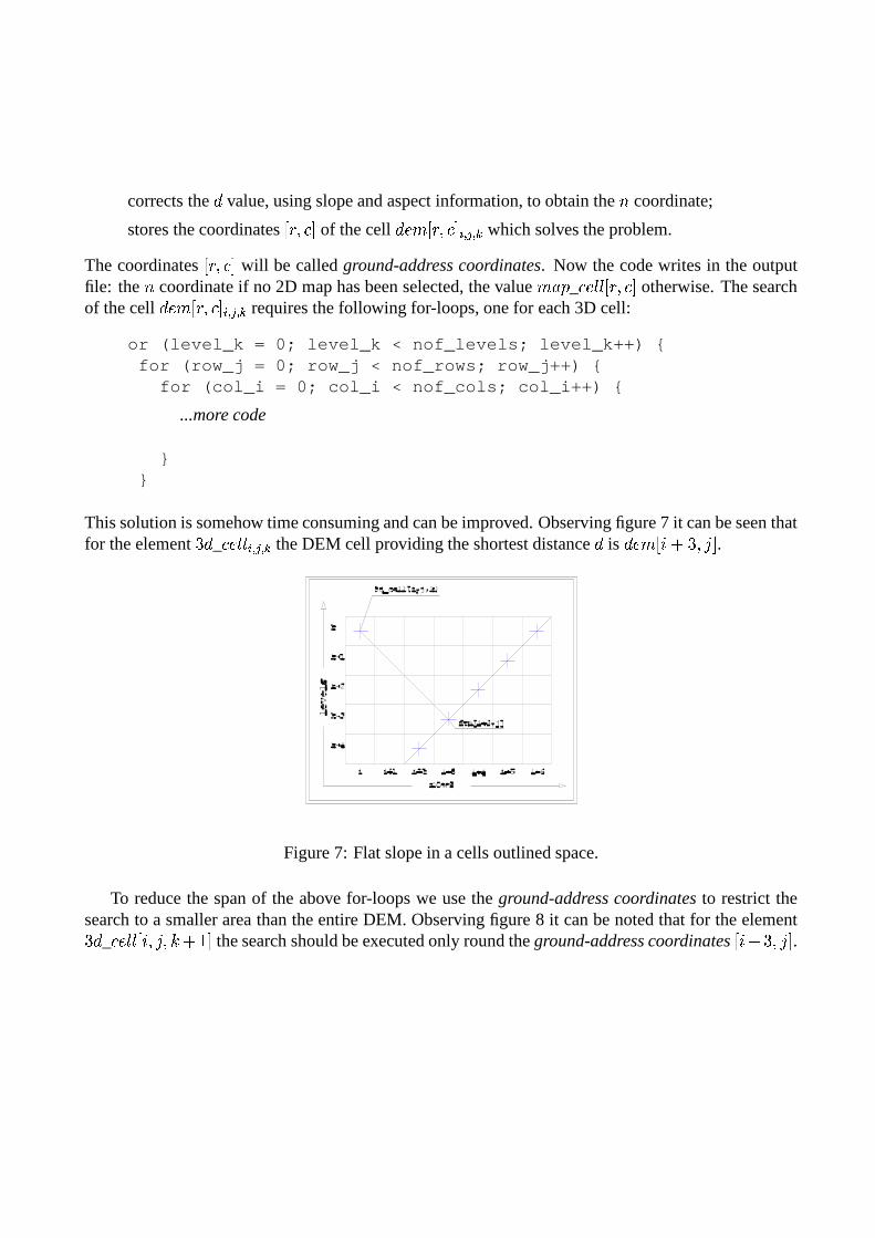
This solution is somehow time consuming and can be improved. Observing figure 7 it can be seen thatfor the element Æ ÷ _ | 7 ��� ±/+ -!+ 6 the DEM cell providing the shortest distance

÷is

÷7 Ë � �*�#Æ ´*) � .

Figure 7: Flat slope in a cells outlined space.

To reduce the span of the above for-loops we use the ground-address coordinates to restrict thesearch to a smaller area than the entire DEM. Observing figure 8 it can be noted that for the elementÆ ÷ _ | 7 ��� � � ´*)�´ r ��¤ � the search should be executed only round the ground-address coordinates � �Û� Æ ´*) � .

Figure 8: Ground-address coordinates outline for a point in the volume.

This approach allows to accelerate the for-loops, executing an aimed search. For the current ele-ment Æ ÷ _ | 7 ��� � � ´*)�´ r � the code only evaluates the distance from the DEM cells inside a window centeredin the ground-address coordinate. The window center is chosen from the ground-address coordinateof the element of coordinates � � ´*)�´ r"p8¤ � , i.e. the element below the current one. For the first level it isnot possible to refer to ground-address coordinate, in this case the ground-address coordinates are setto the current element coordinates. The module allows also to define the dimension of the window, soit is possible to have a quicker search when the slope is almost a slanted plain or when a first solutionis needed, otherwise a larger window can be used to scan a more complex surface. The window ge-ometry depends on the mean aspect of the cells inside the window. For example, if the ground surfaceis south oriented the direction of maximum slope will be north-south oriented, so the window will beoriented along this direction.

5.1.3 Current version

The code, as in the current version, reads the following information from the DEM header and notfrom the set window:

number of rows, cols;

planimetric resolutions;

planimetric limits.

This feature is going to be updated in order to let the user choose between current region and DEMheader setting. Figure 9 is a screen-shot of the module help:

Figure 9: r3.isosurf help and parameters.

where:

dtm 2D raster DEM map name;

aspect 2D raster aspect map name;

slope 2D raster slope map name;

h 3D cells vertical resolution;

[map] 2D raster map to use to obtain a 3D raster map, the value of the 2D map cellbelonging to the normal direction for the 3D cell is assigned to each 3D cell;

output 3D output ASCII file;

[nv] char string to represent no data cell;

[dp] number of decimal places for floats (options: 0-8), default: 8;

[fd] number of cells that defines the dimension of the window scanning the DEM, relativevalue with respect to the window center, must be greater than 0, default: 3;

[tk] number of levels to add over the DEM maximum value.

The module, after writing the output ASCII file, generates an auxiliary ASCII file with the samename of the output file with extension .his. This file contains the list of the parameters used for thisrun.

In figure 10 a geometric configuration it is outlined where for some cells is not possible to defineany normal direction to the ground surface.

Figure 10: Outline of the points without slope normal direction.

Three possible solutions have been provided. A first solution is to leave these particular cellsempty. A second solution is to assign these cells the distance from the surface passing through thenearest point. The third one is to evaluate the � coordinate with respect to slope and aspect informationof the nearest DEM cell.

The code solving these situation is quite simple, and the results are enough good, but it would benecessary a more systematic approach to this problem. To choose the desired method is still necessaryto edit the code and re-compile the module as described in the Grass 5.0 Programmer’s Manual. Analternative solution could be the use of a spatial interpolation algorithm.

5.1.4 Tests and future improvements

The module has been tested on a series of artificial DEM and then applied on a real one. The non-realDEM has been thought to verify the quality of the results. A first slanted plane has been used to mainlyverify the equation (40) which evaluates the � coordinate. An appropriate 2D raster map has also beenused in this first phase to check the correct location of the ground-address coordinates. Another testhas been executed on a more complex DEM built to have a large number of cells for which a normaldirection does not exist.

When the module r3.isosurf has been written the module r3.out.ascii didn’t workproperly. For this reason the module r3.isosurf outputs a file in ASCII format instead of inthe GRASS one. The user has to import the output file of the module r3.isosurf using themodule r3.in.ascii. In this way the user can read the output of the module. Now the mod-ule r3.out.ascii works and the module r3.isosurf will be updated to write directly in theGRASS format.

Of course reading information from the DEM header is not the best solution and the module willbe updated to use the setting of current region instead.

The module now has to be run one time to produce a 3D raster map for the � coordinates andone for each 3D map the user wants to produce from existing 2D raster maps. It would be useful tohave two separate modules. One should produce the 3D raster map with the � coordinates and another

map storing the ground-address coordinates, this is the heavier task, but it must be accomplished onlyonce. Then this second map could be used by the second module to produce as many 3D raster mapas the existing 2D rasters the user wants to input.

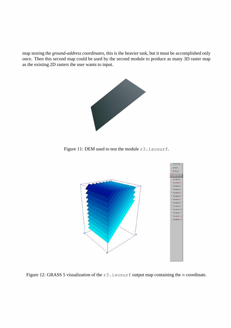
Figure 11: DEM used to test the module r3.isosurf.

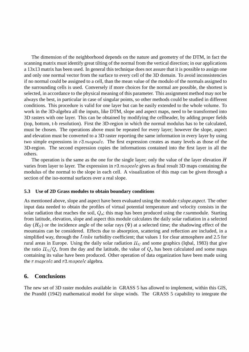
Figure 12: GRASS 5 visualization of the r3.isosurf output map containing the � coordinate.

Figure 13: DEM used to test the module r3.isosurf.

Figure 14: DEM used to test the module r3.isosurf.

Figure 15: GRASS 5 visualization of more surfaces with constant distance from the DEM.

Figure 16: GRASS 5 visualization of more surfaces with constant distance from the DEM.

Figure 17: GRASS 5 visualization of the surface with constant potential temperature [ ½ ], night time.

Figure 18: Slope section and lines with constant potential temperature [ ½ ], night time.

5.2 The normal to the slope: the 3D GRASS maps algebra

Direction and orientation of the surface’s normal are determined by the slope and the aspect of the cellon the DTM; where slope is the side inclination in degrees and aspect is the direction the side is facing,measured with the amplitude of the angle with the east direction. Slope inclination � and aspect 1have been evaluated by the r.slope.aspect GRASS module. A second procedure for calculating themodulus of the normal to the slope will be introduced for a single layer hereafter it will be extendedto the whole 3D volume. By establishing the elevation of the layer in which to calculate the modulus,the point where the perpendicular to the soil, starting from the center of the DTM, intersects the layercan be determined; the value of X and Y, respectively the projection on the x axis and on the y axisof the normal segment N’, can be calculated. First the value of 0 , projection of N’ on the horizontalsurface is calculated (figure 19):

0¡� $�é p21n& ø Ð � � (42)

where é is the height of the layer and 1 is the elevation of the DTM.

Figure 19: Geometric scheme to identify the normal vector starting from the center of the DTM’s cellon a single layer.

Now the values of ü and 3 can be determined:ü �40*|�~:� 1 (43)3¢�50*�I��� 1 (44)

These values are referred to the center of the DTM cell, while the correct distance should be referredto the “atmospheric” cell; some corrections must be introduced to obtain the value of � . By imposing

$%é p61n&87 ³ because the 3D volume is above the DTM, � z can be calculated:� z � $�é p21n&�|�~�� � (45)

The distance between two centers of the cells is a function of the resolution

÷ � and of a parameter, 9 ,that depends on the relative position of the two cells. So the distance | is:|��:9 ÷ � |�~��<$<; p 1 & (46)

where ; is the angle between the line joining the centers and the line indicating the East direction.The modulus of � can be written as: �\� |�>��� � ���>= (47)

And the correction �>= is: �>=¼� � $�é p61n&Äp�$%| ø Ð � 9 R � & � |�~�� � (48)

Finally the value of � is: �\� � 9 ÷ � |�~��<$<; p 1 &©�>��� � � � $%é p61+&�|�~:� � (49)

To implement this procedure in the 3D-GRASS algebra ì ÆNÙ Ë Ð ��| Ð � | , a reference frame needs to be setin order to identify in which cell the normal intersects the layer. The best solution is to center it in the“atmospheric” cell [0,0], the cells on the DTM will be then identified with respect to this reference.For example the cell [-1,1] will have ³N´ Ø ÷ �@? ( ? ¤ ´ Ø ÷ � and ³N´ Ø ÷ �A?4BC? ¤ ´ Ø ÷ � . Starting fromthe “atmospheric” cells the normal to the surface can now be identified: all the cells whose normalspass through the “atmospheric” cell [0,0] are identified by scanning a neighborhood of the central“atmospheric” cell. In this way all the values of � z are evaluated, to these values the correction in theequation (48) must be applied. An example is given in figure 20.

Figure 20: Detection of the normal starting from the “atmospheric” cell.

The dimension of the neighborhood depends on the nature and geometry of the DTM, in fact thescanning matrix must identify great tilting of the normal from the vertical direction; in our applicationsa 13x13 matrix has been used. In general this technique does not assure that it is possible to assign oneand only one normal vector from the surface to every cell of the 3D domain. To avoid inconsistenciesif no normal could be assigned to a cell, than the mean value of the modulo of the normals assigned tothe surrounding cells is used. Conversely if more choices for the normal are possible, the shortest isselected, in accordance to the physical meaning of this parameter. This assignment method may not bealways the best, in particular in case of singular points, so other methods could be studied in differentconditions. This procedure is valid for one layer but can be easily extended to the whole volume. Towork in the 3D-algebra all the inputs, like DTM, slope and aspect maps, need to be transformed into3D rasters with one layer. This can be obtained by modifying the cellheader, by adding proper fields(top, bottom, t-b resolution). First the 3D-region in which the normal modulus has to be calculated,must be chosen. The operations above must be repeated for every layer; however the slope, aspectand elevation must be converted to a 3D raster reporting the same information in every layer by usingtwo simple expressions in ì Æ2Ù Ë Ð �n| Ð � | . The first expression creates as many levels as those of the3D-region. The second expression copies the informations contained into the first layer in all theothers.

The operation is the same as the one for the single layer; only the value of the layer elevation évaries from layer to layer. The expression in ì ÆNÙ Ë Ð ��| Ð � | gives as final result 3D maps containing themodulus of the normal to the slope in each cell. A visualization of this map can be given through asection of the iso-normal surfaces over a real slope.

5.3 Use of 2D Grass modules to obtain boundary conditions

As mentioned above, slope and aspect have been evaluated using the module r.slope.aspect. The otherinput data needed to obtain the profiles of virtual potential temperature and velocity consists in thesolar radiation that reaches the soil,

o ) ; this map has been produced using the r.sunmodule. Startingfrom latitude, elevation, slope and aspect this module calculates the daily solar radiation in a selectedday ( é » ) or the incidence angle of the solar rays ( D ) at a selected time; the shadowing effect of themountains can be considered. Effects due to absorption, scattering and reflection are included, in asimplified way, through the � ����r 7 turbidity coefficient; that values 1 for clear atmosphere and 2.5 forrural areas in Europe. Using the daily solar radiation é » and some graphics (Iqbal, 1983) that givethe ratio é » F o ) from the day and the latitude, the value of

o ) has been calculated and some mapscontaining its value have been produced. Other operation of data organization have been made usingthe ì Ù Ë Ð �n| Ð � | and ì ÆNÙ Ë Ð �n| Ð � | algebra.

6. Conclusions

The new set of 3D raster modules available in GRASS 5 has allowed to implement, within this GIS,the Prandtl (1942) mathematical model for slope winds. The GRASS 5 capability to integrate the

management and the analysis of 3D data with landscape information has been used to apply the Prandtlmodel to an actual 3D domain. An extension of Prandtl’s solution for slope winds has been developedto take in to account evaporation processes so it has been possible to consider the atmosphere as moistand not dry. In both solutions wind velocity depends on the distance of a point in the volume fromthe ground surface measured along the direction normal to the surface. Wind velocity and humidityflux can be derived solving the energy fluxes balance at the ground level. A first complementaryuse of 2D and 3D GRASS modules has been described in this paper. Atmospheric environment hasbeen an ideal application field to test the GRASS 5 3D raster modules. Two different approacheshave been carry out, the first to implement within GRASS the original Prandtl’s solution and thesecond for the extended solution. In the first case a new GRASS module has been written to evaluatethe n coordinate of the points in the entire 3D domain and to transfer 2D information into 3D rastermaps. This approach has been applied to an ideal valley to verify the consistency with the 2D controlmeasurements collected by Defant (1949). In his research Defant measured wind slope velocity in alocation near to Innsbruck (AU) along a uniform valley side, constant slope and aspect angles, constantvegetable cover with stable atmosphere considered as dry. A second application has been developedto a real domain, a site south of Trento in the Adige valley (IT), considering a dry atmosphere. Theresults are in very good accordance with Defant 2D control data and in consistency with expectation.The second approach has been completely developed using the 3D maps algebra exploiting the powerand the flexibility of the module r3.mapcalc. This procedure has been applied first on an idealvalley taking in to account evaporation processes and considering the atmosphere as moist and then,without change atmospheric conditions and features, to the real site south of Trento. Results are inagreement with literature and the sensitivity of the solution to the variation of some parameters hasbeen evaluated. The details of the two procedures and the results are reported in “Proceedings of theOpen source GIS - GRASS users conference 2002 - Trento, Italy, 11-13 September 2002” (Ciolli et al.,2002)

References

Bullini, L., Pignatti, S., Virzo de Santo, A., 1995, Ecologia Vegetale, UTET.

Ciolli, M., Vitti A., Zardi, D., Zatelli, P., 2002, 2D/3D GRASS modules use and development foratmospheric modeling, Proceedings of the Open source GIS - GRASS users conference 2002 -, M.Ciolli, P. Zatelli EDS, Trento, Italy, 11-13 Septesmber 2002.

Ciolli, M., de Franceschi, M., Rea, R., Zardi, D., Zatelli, P., 2002, Modeling of evaporation processesover tiled slopes by means of 3D GRASS raster, Proceedings of the Open source GIS - GRASS usersconference 2002 -, M. Ciolli, P. Zatelli EDS, Trento, Italy, 11-13 Septesmber 2002.

Defant, F., 1949, A theory of slope winds, along with remarks on the theory of mountain winds andvalley winds.

GRASS Development Team, 2001, GRASS 5.0 Programmer’s Manual, www.grass.site.

Iqbal, M., 1983, An introduction to solar radiation, Academic Press.

Monteith, J.L., 1975, Vegetation and the atmosphere, Academic Press.

Monteith, J.L., Unsworth, M.H., 1990, Priples of environmental physics, Edward Arnold.

Prandlt, L., 1942, Essentials of fluid dynamics, Hafner Rib. Comp., NY.

Stull, R.B., 1997, An introduction to Boundary Layer Meteorology, Kluwer Academic Publishers.

Wagner, A., 1923, Zur theorie der berg- und talwinde, Meteorol. Z..

Wagner, A., 1938, Theorie und beobachtung der periodischen gebirgwinde, Gerlands Beitr. Geo-physik, Vol. 52.