Analysing Globalisation and Different Measures of Income Inequality: An ARDL

Approach with Evidence for the OECD Countries

Tiago Manuel Patrício Lindeza

Dissertação para obtenção do Grau de Mestre em

Economia (2º ciclo de estudos)

Orientador: Prof. Doutor José Alberto Serra Ferreira Rodrigues Fuinhas

Co-orientador: Prof. Doutor António Manuel Cardoso Marques

junho de 2020

ii

iii

Acknowledgements

I would like to thank the following people, without whom I would not have been able to

complete this dissertation. My supervisor Prof. Dr. José Alberto Fuinhas, whose

knowledge and guidance into the subject matter drove me through this research. My

friend Tiago for his consistent support and motivation. My parents, who set me off on

the road to this master’s degree a long time ago. My brother for the unconditional love

and support during the compilation of this dissertation. And finally, a special thanks to

my partner, Polina, which the support, encouragement and patience allowed me to

conclude this chapter of my life.

iv

v

Resumo

A desigualdade é um conceito complexo que está associado a um menor crescimento

económico. O coeficiente de Gini tem sido extensivamente aplicado como uma medida

padrão da desigualdade de rendimentos. Portanto, é necessário avaliar a adequação de

medidas alternativas. Este estudo aplica o rácio 20/20 e o rácio Palma como alternativas

ao coeficiente de Gini. A variável da abertura do mercado é estimada como proxy de

globalização. O presente estudo aplica as emissões de CO2, índice de preços ao

consumidor e variáveis de educação como variáveis de controlo. Um painel de dados de

28 países da Organização para a Cooperação e Desenvolvimento Económico foi analisado

usando dados anuais para o período de 1993 a 2014. Três modelos foram estimados e a

abordagem ARDL foi usada para capturar os efeitos de curto e longo prazo. O estimador

Driscoll-Kraay foi utilizado para obter resultados robustos devido à presença do

fenómeno de heterocedasticidade, correlação contemporânea, autocorrelação de

primeira ordem e dependência transversal. Os resultados sugerem que a globalização

aumentou a desigualdade de rendimentos, enquanto as emissões de CO2 e o índice de

preços ao consumidor causaram um impacto negativo na desigualdade de rendimentos,

ou seja, promovem a igualdade de rendimentos. Esta evidência deve ser considerada na

definição de estratégias de desigualdade, especificamente tornando a globalização

compatível com a mitigação da desigualdade de rendimentos.

Palavras-chave

Desigualdade de Rendimentos; Globalização; Rácio 20/20; Rácio Palma; ARDL

vi

vii

Resumo Alargado

O aumento da desigualdade de rendimentos é um dos desafios do nosso tempo, que, caso

não seja abordado adequadamente, pode levar ao aparecimento de catástrofes políticas

e sociais. Apesar do modo como a desigualdade de rendimentos é medida seja uma

consideração relevante para a criação de políticas a favor do crescimento económico de

um país, ainda não há consenso na sua medição. O coeficiente de Gini, que varia entre 0

e 1, sendo zero a igualdade perfeita e um a desigualdade máxima, tem sido

extensivamente aplicado como uma medida padrão de desigualdade de rendimentos.

Portanto, é necessário avaliar a adequação de medidas alternativas. Este estudo aplica

como alternativas ao coeficiente de Gini, o rácio 20/20, que compara a riqueza dos 20%

da população mais rica com a riqueza dos 20% mais pobres, e o rácio Palma, que compara

a riqueza dos 10% mais ricos com a dos 40% mais pobres. O aumento da globalização nas

últimas décadas tem vindo a ser associado ao aumento das desigualdades de rendimento.

É necessário então estudar e analisar a relação entre desigualdade de rendimentos e

globalização com o objetivo de se criar medidas de política económica para contrariar os

seus efeitos indesejados. Semelhante à desigualdade de rendimentos, também não existe

consenso no modo de medir a globalização. Neste caso, a globalização pode ser definida

em características sociais, económicas e políticas. Este estudo foca-se na característica

económica e estima a variável da abertuda do mercado como proxy da globalização.

Este trabalho tem como objectivo contribuir para a literatura atual, medindo o grau de

impacto da globalização na desigualdade de rendimentos no curto e no longo prazo para

os países membros da Organização para a Cooperação e Desenvolvimento Económico.

Adicionalmente, é também feito o estudo do impacto de outros indicadores na

desigualdade de rendimentos no curto e no longo prazo.

Para a elaboração do estudo, foi analisado um painel de dados de 28 países pertencentes

à OCDE, usando dados anuais para o período de 1993 a 2014. Como proxy da

desigualdade de rendimentos, foi criado um modelo explicativo para cada uma das

medidas de desigualdade analisadas, coeficiente de Gini, rácio 20/20 e rácio Palma.

Como variáveis dependentes foram utilizadas, as emissões de dióxido de carbono em per

capita com o propósito de estudar o impacto das alterações climáticas na desigualdade

de rendimentos; o índice de preços ao consumidor que reflete as tendências de inflação;

a matrícula escolar secundária como proxy da educação e representa a população total

matriculada no ensino médio. O conjunto de dados foi então submetido a uma bateria de

viii

testes para analisar as suas propriedades e garantir que o estimador mais adequado é

utilizado. Devido à presença do fenómeno de heterocedasticidade, correlação

contemporânea, autocorrelação de primeira ordem e dependência transversal, o

estimador Driscoll-Kraay foi utilizado para obter resultados robustos. A abordagem

ARDL, ao suportar variáveis estacionárias em nível e também nas suas primeiras

diferenças, foi usada para capturar os feitos de curto e longo prazo. Os resultados desta

investigação revelam grande consistência com a literatura e a teoria económica ao sugerir

que o aumento da globalização aumenta a desigualdade de rendimentos, enquanto o

aumento das emissões de CO2 e de o índice de preços ao consumidor, causa um impacto

negativo na desigualdade de rendimentos, ou seja, promovem a igualdade de

rendimentos. As principais conclusões do estudo sugerem então implicações políticas

importantes para reduzir a desigualdade de rendimentos. Relativamente à globalização,

os resultados sugerem que deve ser considerado a implementação de sistemas

redistributivos como, por exemplo, o programa Transferências Condicionais de

Rendimentos. Como o aumento do índice de preços ao consumidor causa uma

diminuição da desigualdade de rendimentos, os países membros da OCDE, através dos

bancos centrais, devem continuar a manter o controlo dos níveis de inflação. No que diz

respeito às alterações climáticas, as medidas a ser implementendas devem considerar o

trade-off entre desigualdade de rendimentos e as emissões de CO2. Um exemplo de uma

medida que possa ser implementada e poderia resolver este trade-off, é um imposto de

carbono redistributivo, neutro em receitas. Este imposto iria incentivar a redução de

emissões de dióxido de carbono, e simultaneamente, redistribuir as receitas para o

melhoria dos serviços públicos usados por famílias pertencentes à classe baixa de

rendimentos.

ix

x

Abstract

Inequality is a complex concept that is associated with lower economic growth. The Gini

coefficient has been extensively applied as a standard measure of income inequality.

Therefore, there is a need to assess the appropriateness of alternative measures. This

study applies the 20/20 ratio and Palma ratio as alternatives to the Gini Coefficient. The

trade openness variable as a globalisation proxy is assessed. The present study applies

CO2 emissions, consumer price index and education variables as control variables. A

panel data of 28 countries from the Organization for Economic Co-operation and

Development was analysed using annual data for the period from 1993 to 2014. Three

models were estimated, and the ARDL approach was used to capture the short- and long-

run effects. The Driscoll-Kraay estimator was used to attain robust results, given the

presence of the phenomena of heteroscedasticity, contemporaneous correlation, first-

order autocorrelation and cross-sectional dependence. Results suggest that globalisation

has increased income inequality, while CO2 emissions and consumer price index have

impacted income inequality negatively, i.e., promote income equality. This finding

should be incorporated into the definition of inequality strategies, specifically by making

globalisation compatible with income inequality mitigation

Keywords

Income Inequality; Globalisation; 20/20 Ratio; Palma Ratio; ARDL

xi

xii

Contents

Acknowledgements ......................................................................................................... iii

Resumo .............................................................................................................................. v

Palavras-chave................................................................................................................... v

Resumo Alargado ............................................................................................................ vii

Abstract ............................................................................................................................. x

Keywords ........................................................................................................................... x

Contents .......................................................................................................................... xii

Figures List ..................................................................................................................... xiv

Tables List ...................................................................................................................... xvi

Acronymous List .......................................................................................................... xviii

1. Introduction ................................................................................................................... 1

2. Literature Review .......................................................................................................... 4

3. Data and Methodology ................................................................................................ 10

3.1. Description of the data ......................................................................................... 10

3.2. Methodology ........................................................................................................ 12

4. Results ......................................................................................................................... 17

5. Discussion.................................................................................................................... 22

6. Conclusion ................................................................................................................... 24

References ....................................................................................................................... 25

xiii

xiv

Figures List

Figure 1. Inequality during the Industrial Revolution and the rise of the West ............... 1

Figure 2. Percentiles of the global income distribution .................................................... 7

xv

xvi

Tables List

Table 1. Descriptive statistics and cross-sectional dependence. ..................................... 17

Table 2. Second generation unit root tests. ..................................................................... 18

Table 3. Westerlund cointegration test. .......................................................................... 18

Table 4. Hausman and Specification tests. ..................................................................... 19

Table 5. Estimation Results for Palma model. ................................................................ 19

Table 6. Estimation Results for 20/20 model. ................................................................ 20

Table 7. Estimation Results for Gini model. ................................................................... 20

Table 8. Short-run impacts and elasticities. ................................................................... 21

xvii

xviii

Acronymous List

CO2 Carbon Dioxide Emissions

ARDL Autoregressive Distributed Lag

OECD Organisation for Economic Co-operation and Development

EHII Estimated Household Income Inequality

GMM Generalised Method of Moment

FDI Foreign Direct Investment

EU European Union

SWWID Standardised World Income Inequality Database

WID World Inequality Database

GDP Gross Domestic Product

VIF Variance Inflation Factor

CIPS Cross-Section Im-Pesaran-Shin

CADF Cross-sectionally Augmented Dickey-Fuller

MG Mean Group

PMG Pooled Mean Group

RE Random Effect

FE Fixed Effect

PCS Panel-Corrected Standard Errors

OLS Ordinary Least Squares

ECM Error Correction Mechanism

xix

1

1. Introduction

Rising income inequality is a widespread concern and the defining challenge of our time,

when, not properly addressed, it leads to the appearance of political and social catastrophes.

Due to the increase of globalisation in the last 30 years, there is a need to study and analyse

the inequality-globalisation relationship.

According to Bourguignon & Morrisson (2002), inequality strongly intensified during

Industrial Revolution and rise of the West (Figure 1), i.e., that not only inequality between

individuals is much higher today than 200 years ago, but inequalities’ composition has also

been totally reversed from being predominantly driven by within-national inequalities, to

be determined by the differences in mean country incomes (Milanovic, 2011).

The increase in global mean income combined with the increase in global inequality, made

the global inequality extraction ratio, the ratio between actual Gini and maximum feasible

Gini which can be interpreted as the share of maximum inequality extracted by the elite

(Milanovic et al., 2011), be broadly stable in the last century. This means that during the last

100 years, World War Two and United States dominance, global inequality has increased

on the same rate as the maximum feasible inequality, stagnating the global inequality

extraction ratio around 70% (Milanovic, 2011). Moreover, more recently, during the rise of

Asia, decline moderately.

Figure 1. Inequality during the Industrial Revolution and the rise of the West

(Source: Lakner and Milanovic (2013))

Year

Gin

i in

dex

2

The measure of inequality is a relevant consideration in which there is still no consensus,

and it can be divided into global and partial measures. Global measures include Atkinson

index, Generalised Entropy Indices or the Gini coefficient. In contrast, the Palma ratio, the

share of the bottom 40% or 20/20 ratio can be designated as partial measures for not

accounting full distribution. This research will focus on the standard measure of inequality

such as Gini Coefficient, where its range is between 0 and 1, perfect equality and maximum

inequality, respectively. Along with the two most used ratios, 20/20 and Palma. While the

20/20 ratio compares the wealth of the 20% wealthiest with the wealth of the 20% poorest

individuals, the Palma ratio compares the wealth of the top 10% with the bottom 40%.

As noted above, there was a generalised increase in the world’s globalisation levels in the

last three decades. Similar to measuring inequality, there still is a lack of consensus in the

measure of globalisation. Considering multidimensional globalisation characteristics,

several studies (Keohane & Nye, 2000; Fuinhas & Marques, 2017) accept economic, political

and social as the main dimensions to study globalisation. However, the economic

characteristic of globalisation is the most extensively applied. As economic characteristics,

measuring globalisation includes trade openness, foreign direct investment, financial flows

and migration across national borders. As most studies that focus on economic

characteristics to determine globalisation, this research will apply trade openness as a proxy

of globalisation. Considering trade openness as a measure of globalisation is an advantage

in the study of the relationship between globalisation and income inequality. Although trade

openness has been associated with economic growth, in the income inequality spectrum,

trade’s impact it still is controversial. As several studies (Marjit & Acharyya, 2003; Chiquiar,

2008) predict that the wage gap between skilled and unskilled labour should be decreased

due to trade openness, proceeding to a decrease in inequality. On the other side of the

spectrum, disparities in returns to education and skills may arise an increase of income

inequality.

This paper aims to study globalisation and different measures of inequality for the countries

of Organisation for Economic Co-operation and Development (OECD). The relevance of this

study is high since these countries share common goals such as promoting economic

growth, prosperity and sustainable development. Also, seeing if the implemented strategies

are leading the countries members of OECD to the decrease of inequality reveals further

importance of this paper. Additionally, this research aims to check the impact of climate

change, education and inflation on income inequality. A panel ARDL model will be applied

to perform the analysis. This method allows for a different integration order of variables,

such as I(0) and I(1) and it is able to provide estimations of the inequality drivers for the

short and long run, simultaneously.

3

The main objective of this study is to contribute to the existent literature by estimating the

degree of globalisation impact on income inequality in the short and long run for the

countries members of the OECD. A secondary objective was added, to estimate the

magnitude of other inequality drivers in the short and long run, also for OECD countries.

This study is organised as follows. Section 2 presents the literature review, which analyses

the main existing investigations on this subject. Section 3 presents the data and

methodology, where the variables and models to be estimated are presented. The results of

this study are presented in section 4 and discussed in section 5. Finally, section 6 presents

the main conclusions of the study and proposals for future research.

4

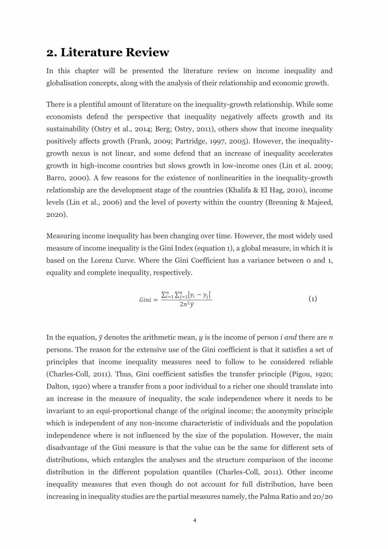
2. Literature Review

In this chapter will be presented the literature review on income inequality and

globalisation concepts, along with the analysis of their relationship and economic growth.

There is a plentiful amount of literature on the inequality-growth relationship. While some

economists defend the perspective that inequality negatively affects growth and its

sustainability (Ostry et al., 2014; Berg; Ostry, 2011), others show that income inequality

positively affects growth (Frank, 2009; Partridge, 1997, 2005). However, the inequality-

growth nexus is not linear, and some defend that an increase of inequality accelerates

growth in high-income countries but slows growth in low-income ones (Lin et al. 2009;

Barro, 2000). A few reasons for the existence of nonlinearities in the inequality-growth

relationship are the development stage of the countries (Khalifa & El Hag, 2010), income

levels (Lin et al., 2006) and the level of poverty within the country (Breuning & Majeed,

2020).

Measuring income inequality has been changing over time. However, the most widely used

measure of income inequality is the Gini Index (equation 1), a global measure, in which it is

based on the Lorenz Curve. Where the Gini Coefficient has a variance between 0 and 1,

equality and complete inequality, respectively.

𝐺𝑖𝑛𝑖 = ∑ ∑ |𝑦𝑖 − 𝑦𝑗| 𝑛

𝑗=1𝑛𝑖=1

2𝑛2�̅� (1)

In the equation, �̅� denotes the arithmetic mean, y is the income of person i and there are n

persons. The reason for the extensive use of the Gini coefficient is that it satisfies a set of

principles that income inequality measures need to follow to be considered reliable

(Charles-Coll, 2011). Thus, Gini coefficient satisfies the transfer principle (Pigou, 1920;

Dalton, 1920) where a transfer from a poor individual to a richer one should translate into

an increase in the measure of inequality, the scale independence where it needs to be

invariant to an equi-proportional change of the original income; the anonymity principle

which is independent of any non-income characteristic of individuals and the population

independence where is not influenced by the size of the population. However, the main

disadvantage of the Gini measure is that the value can be the same for different sets of

distributions, which entangles the analyses and the structure comparison of the income

distribution in the different population quantiles (Charles-Coll, 2011). Other income

inequality measures that even though do not account for full distribution, have been

increasing in inequality studies are the partial measures namely, the Palma Ratio and 20/20

5

Ratio. Supporting this last statement, according to Cobham & Sumner (2013), between

Palma Ratio and Gini Coefficient, Palma is a more useful measure of inequality for

policymakers and citizens to track.

𝑃𝑎𝑙𝑚𝑎 𝑅𝑎𝑡𝑖𝑜 = �̅�𝑖𝑡𝑜𝑝10

�̅�𝑖𝑏𝑜𝑡𝑡𝑜𝑚40

(2)

While the Palma Ratio (equation 2) compares the share of the wealth (�̅�) of the top 10%

with the share of the wealth of the bottom 40% (Palma, 2006; Palma, 2011), the 20/20 Ratio

(equation 3) focuses on the comparison of the wealth of the 20% wealthiest individuals

(𝑖) with the wealth of the 20% poorest individuals of the population. Meanwhile, for a

detailed comparison between these income inequality measures, we can follow the work of

Pascoal & Rocha, (2018).

20/20 𝑅𝑎𝑡𝑖𝑜 = �̅�𝑖𝑡𝑜𝑝20

�̅�𝑖𝑏𝑜𝑡𝑡𝑜𝑚20

(3)

Although literature focusing inequality has been extensively analysed on different branches,

there is no consensus on its outcomes and determinants. Indeed, regarding the financial

branch, there are studies where high levels of financial development, financial liberalisation

and the occurrence of a banking crisis, increase income inequality in a country (de Haan &

Sturm, 2017), contradicting the work seen in Bumann and Lensink (2016). Although the

focus of our study is the globalisation-inequality nexus, we will also study other indicators

that are often discussed in the literature. Following the Kuznets Curve hypothesis (Kuznets,

1995) that postulates an inverted U-shaped relation between per capita income and

inequality and given the urgency of the climate change challenge, several studies focused on

the impact of income inequality on CO2 emissions (Hubler, 2017; Liu et al., 2019). However,

according to Ravallion et al. (2000) there is a need to address to a trade-off between them.

In the manner that inequality-growth relationship may present nonlinearities due to

income levels (Lin et al., 2006), the tradeoff between inequality and carbon emissions also

depends on income levels (Grunewald et al., 2017); low and middle-income economies,

higher income inequality is associated with lower carbon emissions while in upper-middle-

income and high-income economies, higher income inequality increases per capita

emissions (Grunewald et al., 2017).

According to Goldin & Katz (2007), human capital is an important determinant of income

inequality because of higher returns to education. As education determines access to jobs,

6

pay levels and takes part as a key role as an indication of ability and productivity in the job

market, education plays an important role in income inequality. Education literature

suggests that the effect on income inequality could be positive or negative, depending on

the evolution of rates of return to education, that is, the skill premium (Dabla-Norris et al.,

2015). Interestingly, in advanced economies, higher skill premium is associated with

widening inequality while in economically more developed countries, skill premium is

statistically insignificant (Dabla-Norris et al., 2015).

Similarly, to socio-economic characteristics as education, fiscal and monetary policies, e.g.,

inflation and consumer price index, are also important determinants of income inequality.

As low-income households are generally more vulnerable to increases in the price level as

they have a higher portion of cash in total purchases (Albanesi, 2007) relative to other

financial assets than high-income households (Erosa & Ventura, 2002). To support the

importance of inflation, Easterly and Fischer (2001) present indirect evidence of the

distributional consequences of inflation, demonstrating that low-income households are

more likely to mention inflation as a top concern.

Turning to the other subject of analysis and the main focus of our study, the globalisation-

inequality relationship, we can start by stating that as a progressively globalised world, there

has been an exceptional increase in the globalisation research, helping policymakers in the

development of growth-promoting policies.

When discussing the way globalisation affects growth, it is important to distinguish between

theoretically and empirically. According to Grossman & Helpman (2015), theoretical

literature identifies several different possible relations between globalisation and growth.

Meanwhile, empirically, even though literature points its positive effect on growth (Fuinhas

& Marques, 2017; Gurgul & Lach, 2014), there still is a lack of consensus in this

globalisation-growth nexus. The main reason for this, it is defining and measuring

globalisation, formulating that globalisation has a multidimensional characteristic (Dreher,

2006). Supporting the challenge of measuring globalisation, in previous studies, trade

openness (Frankel & Romer, 1999) and foreign direct investment (Dollar & Kraay, 2001)

are used as proxies. Nowadays, accounting the multidimensional globalisation

characteristic and accepting economic, political and social as the main dimensions,

researchers use as a proxy of globalisation, the Konjunkturforschungsstelle (KOF) Index of

Globalisation (Fuinhas & Marques, 2017).

The studies focused on globalisation-inequality relationship, usually use as a proxy the

economic characteristics, namely, the trade openness and foreign direct investment, in

7

which, Kraay (2006) found a strong positive link between trade openness and inequality.

According to Asteriou et al. (2014), the financial crisis led to a rise in inequality and the

policies to mitigate inequality should be in regards to foreign direct investment.

Focusing on trade, it has been an engine for growth in many countries by promoting

competitiveness and enhancing efficiency. Standard trade theory, as Stolper-Samuelson

theorem, predicts that trade openness, through tariff reduction, should reduce the wage gap

between skilled and unskilled labour in developing countries, resulting in a reduction of

income inequality (Asteriou et al., 2014). Meanwhile, on advanced economies, due to

disparities in returns to education and skills, trade may aggravate income inequality

(Stiglitz, 1998). Other studies also state that income inequality increases with an increase

in trade openness (Kanbur, 2015) and the disequalising effects of trade openness decrease

as a country grows (Hamori & Hashiguchi, 2012).

Nowadays, still inside the income inequality spectrum, it is already possible to determine

who had the largest and smallest gains of globalisation when analysing the changes in real

incomes (Lakner and Milanovic, 2013). Figure 2 shows the change in real income between

1988 and 2008 at various percentiles of the global income distribution. One can state that

in the past two decades of globalisation, the parts of global income distribution registered

the largest gains are the very top of the global income distribution and among the middle

classes of emerging market economies.

Figure 2. Percentiles of the global income distribution (Source: Lakner and Milanovic (2013))

Percentiles of global income distribution

Cum

ula

tive g

row

th r

ate

%

8

As Figure 2 demonstrates, over those two decades, the top 1% has seen its real income

strongly intensify by more than 60%. However, the biggest increase was registered around

the 50th and 60th percentile, reaching an 80% real income increase. On the other side,

other than the poorest 5%, the ones that registered the smallest gains, are between the 75th

and 90th percentiles of the global income distribution, in which the real income gains were

none. Following Milanovic (2013), global income distribution has thus changed remarkably

and was probably the most profound global reshuffle of people’s economic positions.

Even though we are covering some characteristics in the existing ample literature on the

relationships inequality-growth and globalisation-growth, as we stated previously, the focus

of our study is the globalisation-inequality nexus. When analysing each relationship

empirically, we reckon that, in inequality-growth, utmost studies have as a focal point, the

financial branch, more specifically, financial development and financial liberalisation. For

instance, Furceri and Loungani (2015) demonstrated that financial liberalisation increases

inequality with fixed effects method on 149 countries from 1970 to 2010. Jauch and Watzka

(2015) demonstrated that more financial development leads to more inequality when

controlling for country and time fixed effects, with an unbalanced dataset of up to 138

developed and developing countries over the years from 1960 to 2008. Additionally, using

random effects and cross-country regressions for a sample of 121 countries covering 1975-

2005, de Hann & Sturm (2017) shows that all finance variables increase income inequality.

Regarding the globalisation-growth relationship, the use of panel data techniques is also

becoming more usual on empirical studies, since it has a vast number of advantages over

the cross-sectional, and time-series analysis (Hsiao, 2007). Moreover, some studies are

handling globalisation as an endogenous variable, strongly increasing the use of dynamic

estimators. For example, as per the work of Hamori & Hashiguchi (2012) that studies the

effect of financial deepening on inequality. Through a panel data set of 126 countries for the

period 1963-2002 and using estimated household income inequality (EHII) data as an

inequality measure, demonstrated that inequality increases with an increase in trade

openness. The researchers performed a Hausman test in order to choose a fixed-effect

model over a random-effect model (Hausman, 1978). Also, a regression with white cross-

section robust standard errors was executed to consider heteroskedasticity in the error

terms. In order to deal with the endogeneity problem, they estimated each model using the

panel dynamic generalised method of moment (GMM) estimators developed by Arellano

and Bond (1991), resulting in the same findings previously achieved. Supporting the use of

dynamic estimators, we can also follow the work of Asteriou et al. (2014), for the period

from 1995 to 2009 and the set of 27 European Union countries. A panel regression was

estimated in order to explain income inequality measured by the log of the Gini coefficient

9

as a function of globalisation measures, trade openness and foreign direct investment. For

reasons of robustness, but also in order to consider any dynamic effect and endogeneity

problems, the estimation was repeated with the use of the GMM method. Although the

results display a reduction in inequality from trade openness in the EU-27, the highest

contribution to the average change of inequality comes from FDI. Results are consistent

with the fixed effects estimator, suggesting that the results are robust.

Although there is a vast literature that analyses the inequality-growth, globalisation-growth

and globalisation-inequality relationships, there is still no consensus, and the discussion

about the results remains ambiguous. The econometric techniques, the timespan and

sample that researchers choose, may be the main reasons for the diversity seen in the

results. Additionally, the globalisation dimensions included in their estimations may also

be one reason for the lack of consensus in this matter.

10

3. Data and Methodology

The following chapter is divided in two sections. The first will identify and describe the

variables used, along with the sample and timespan. The second section will describe the

methodology and reveal the models used.

3.1. Description of the data

For this study, it was used a panel dataset with annual frequency for the period from 1993

to 2014 for twenty-eight (28) countries belonging to the Organisation for Economic Co-

operation and Development (OECD). The selected countries are the followings: Austria,

Belgium, Czech Republic, Denmark, Estonia, Finland, France, Germany, Greece, Hungary,

Iceland, Ireland, Italy, Latvia, Lithuania, Luxembourg, Netherlands, Norway, Poland,

Portugal, Slovak Republic, Slovenia, Spain, Sweden, Switzerland, Turkey, United Kingdom

and the United States. Based on data availability criteria, the remaining OECD member

countries were excluded. As members of OECD, the countries share the common goal of

fostering economic development and co-operation, contributing to the expansion of world

trade and promoting economic stability.

Three different variables are used as proxies of income inequality to reach the purpose of

analysing globalisation and different measures of income inequality:

- GC: Gini index of disposable income from the Standardised World Income

Inequality Database (SWIID). As a standard measure of income inequality, the Gini

Coefficient has been extensively applied in the inequality literature, for example, in

the work of Santiago et al. (2019). For more information in regards the SWIID, we

can follow Solt (2016).

- PR: Palma ratio has been increasing in inequality studies (Cobham & Sumner 2013).

The source of this variable is the World Inequality Database (WID) and consists in

dividing the share of income, in constant local and base 2008, from the top 10%

(p90-p100) per the bottom 40% (p0-p40).

- TTR: 20/20 ratio as an alternative to the Palma Ratio. The source is also the World

Inequality Database (WID) and consists in dividing the share of income, in constant

local and base 2008, from the top 20% (p80-p100) per the bottom 20% (p0-p20).

Follow Pascoal & Rocha (2018) for a detailed comparison between these measures.

Accounting the economic characteristics, in order to analyse globalisation, the following

variable is used as a proxy:

11

- T: Trade openness as a percentage (%) of GDP is the sum of exports and imports of

goods and services measured as a share of gross domestic product. This variable was

extracted from the World Bank and is one of the most common measures of

globalisation, seen in plentiful literature as per example, Asteriou et al. (2014).

The source of the control variables was the World Development Indicators (WDI) published

by the World Bank, namely:

- CO2: Carbon dioxide emissions, per capita, covers emissions from fossil fuel, natural

gas and cement manufacturing. Due to the climate change challenge, CO2 emissions

per capita has been used, in previous studies as Grunelwald et al. (2017), to research

the relationship between income inequality and environmental degradation.

- CPI: Consumer price index, base 2010, reflects variations in the cost to the average

consumer of acquiring goods and services that may be fixed or changed at specified

intervals, such as yearly. This variable is generally calculated by the Laspeyres

formula and is used mainly in the financial branch inside the inequality spectrum as

in Kim et al. (2011).

- EDUC: School enrollment, secondary (% gross) represents the total population

enrolled at the secondary school level, which completes the provision of basic

education, offering additional subjects and skills, along with more specialised

teachers. This variable is used as a proxy of education in the inequality literature as

in Bumann & Lensink. (2016).

12

3.2. Methodology

A battery of tests was implemented in order to achieve the purpose of this research, using

the econometric software Stata15. As such, to check the adequacy of the data for the use of

panel data techniques, the Variance Inflation Factors (VIF) test was executed to verify the

existence of linear relationships between the variables. As three different income inequality

measures were used, Gini coefficient, Palma ratio and 20/20 ratio, the VIF test is performed

for every one of them. The absence of multicollinearity is proved by low VIF statistic values,

resulting in a similar mean VIFs of 1.20.

Considering that the sample is based on OECD countries, common shocks are expected, for

instance, financial crisis and common policies. To investigate the presence of cross-

sectional dependence in each variable, the CD-test developed by Pesaran (2004) was

applied. Panel data are a sequence measure of individuals or countries (i) over time (t). A

regression and tests are constructed on a dependent variable (𝑦𝑖𝑡) and a set of independent

variables (𝑋′𝑖𝑡) for I= 1,..., N and t=1,..., T. The CD-test specification is represented in

following Eq. (4)

𝐶𝐷 = √2𝑇

𝑁(𝑁 − 1)(∑ ∑ 𝜌𝑖𝑗

𝑁

𝑗=𝑖+1

𝑁−1

𝑖=1

) (4)

where 𝜌𝑖𝑗 is the autocorrelation coefficient. The CD-test is performed under the null of

cross-sectional independence.

Considering the presence of cross-sectional dependence, a first-generation panel unit root

test is no longer robust to assess the stationary properties of the variables. A second-

generation unit root test was applied to verify the integration order of the variables. The

Cross-Section Im-Pesaran-Shin (CIPS) test, proposed by Pesaran (2007), is based on a

cross-sectionally augmented Dickey-Fuller (CADF) regression and allowed the presence of

a single unobserved common factor under the null hypothesis of non-stationarity.

Accordingly, H0: 𝑏𝑖 = 0 for all i. The CADF regression is represented in following Eq. (5)

∆𝑦𝑖𝑡 = 𝛼𝑖 + 𝑏𝑖𝑦𝑖,𝑡−1 + 𝑐𝑖�̅�𝑡−1 + 𝑑𝑖∆�̅�𝑡 + 휀𝑖𝑡 (5)

where ∆ denotes the first difference operator, �̅� is the mean of y and 휀 denotes the error

term.

13

In order to examine the absence of cointegration by determining whether there exists error

correction for individual panel members (Gt and Ga) or the panel as a whole (Pt and Pa),

the Westerlund test was applied. The second-generation cointegration test developed by

Westerlund (2007) uses bootstrapping to obtain robust critical values. The statistics of Gt,

Ga, Pt and Pa, are obtained by the Eq. (6), Eq. (7), Eq. (8) and Eq. (9), respectively.

𝐺𝑡 = 1

𝑁∑

𝜃𝑖

𝑆𝐸(𝜃𝑖)

𝑁

𝑖=1

(6)

𝐺𝑎 = 1

𝑁∑

𝑇𝜃𝑖

𝜃′(1)

𝑁

𝑖=1

(7)

𝑃𝑡 = 𝜃𝑖

𝑆𝐸(𝜃𝑖) (8)

𝑃𝑎 = 𝑇𝜃 (9)

In the equations, 𝜃 denote error correction parameter, and SE stands for standard deviation.

The null hypothesis for the Westerlund test is for all statistics H0: 𝜃𝑖= 0 for all i. Since the

cointegration test determines how the variables are introduced into the model, if the

presence of cointegration is observed, the variables are used at the level, if not, the first

differences are applied.

In the interest of the study between the globalisation and income inequality relationship, it

is beneficial to examine the dynamic effects separately in the short and long run. The

Autoregressive Distributed Lag (ARDL) model allows examining the long and short-run

impact of independent variables on the dependent ones. This estimator also allows for a

different integration order of variables, as I(0) and I(1) but not I(2). The heterogeneous

estimators, such as Mean Group (MG) and Pooled Mean Group (PMG) were not tested or

considered due to the reason that the sample is composed of OECD countries. A

homogeneous panel should be considered. As stated previously, the Gini coefficient, Palma

ratio and 20/20 ratio are used as inequality measures, acknowledging the dependent

variables for equations (10), (11) and (12), respectively. The following equations represent

the ARDL models, where the short and long-run dynamics can be observed:

14

𝐷𝐿𝐺𝐶𝑖𝑡 = 𝛼𝑖 + ∑ 𝛽1𝑖𝑗

𝑘

𝑗=1

𝐷𝐿𝐺𝐶𝑖𝑡−𝑗 + ∑ 𝛽2𝑖𝑗

𝑘

𝑗=0

𝐷𝐿𝑇𝑖𝑡−𝑗 + ∑ 𝛽3𝑖𝑗

𝑘

𝑗=0

𝐷𝐿𝐶𝑂2𝑖𝑡−𝑗

+ ∑ 𝛽4𝑖𝑗

𝑘

𝑗=0

𝐷𝐿𝐶𝑃𝐼𝑖𝑡−𝑗 + ∑ 𝛽5𝑖𝑗

𝑘

𝑗=0

𝐷𝐿𝐸𝐷𝑈𝐶𝑖𝑡−𝑗 + 𝜆1𝑖𝐿𝐺𝐶𝑖𝑡−1

+ 𝜆2𝑖𝐿𝑇𝑖𝑡−1 + 𝜆3𝑖𝐿𝐶𝑂2𝑖𝑡−1 + 𝜆4𝑖𝐿𝐶𝑃𝐼𝑖𝑡−1 + 𝜆5𝑖𝐿𝐸𝐷𝑈𝐶𝑖𝑡−1 + 휀𝑖𝑡

(10)

𝐷𝐿𝑃𝑅𝑖𝑡 = 𝛼𝑖 + ∑ 𝛿1𝑖𝑗

𝑘

𝑗=1

𝐷𝐿𝑃𝑅𝑖𝑡−𝑗 + ∑ 𝛿2𝑖𝑗

𝑘

𝑗=0

𝐷𝐿𝑇𝑖𝑡−𝑗 + ∑ 𝛿3𝑖𝑗

𝑘

𝑗=0

𝐷𝐿𝐶𝑂2𝑖𝑡−𝑗

+ ∑ 𝛿4𝑖𝑗

𝑘

𝑗=0

𝐷𝐿𝐶𝑃𝐼𝑖𝑡−𝑗 + ∑ 𝛿5𝑖𝑗

𝑘

𝑗=0

𝐷𝐿𝐸𝐷𝑈𝐶𝑖𝑡−𝑗 + 𝜔1𝑖𝐿𝑃𝑅𝑖𝑡−1

+ 𝜔2𝑖𝐿𝑇𝑖𝑡−1 + 𝜔3𝑖𝐿𝐶𝑂2𝑖𝑡−1 + 𝜔4𝑖𝐿𝐶𝑃𝐼𝑖𝑡−1 + 𝜔5𝑖𝐿𝐸𝐷𝑈𝐶𝑖𝑡−1 + 𝜇𝑖𝑡

(11)

𝐷𝐿𝑇𝑇𝑅𝑖𝑡 = 𝛼𝑖 + ∑ 𝛾1𝑖𝑗

𝑘

𝑗=1

𝐷𝐿𝑇𝑇𝑅𝑖𝑡−𝑗 + ∑ 𝛾2𝑖𝑗

𝑘

𝑗=0

𝐷𝐿𝑇𝑖𝑡−𝑗 + ∑ 𝛾3𝑖𝑗

𝑘

𝑗=0

𝐷𝐿𝐶𝑂2𝑖𝑡−𝑗

+ ∑ 𝛾4𝑖𝑗

𝑘

𝑗=0

𝐷𝐿𝐶𝑃𝐼𝑖𝑡−𝑗 + ∑ 𝛾5𝑖𝑗

𝑘

𝑗=0

𝐷𝐿𝐸𝐷𝑈𝐶𝑖𝑡−𝑗 + 𝜃1𝑖𝐿𝑇𝑇𝑅𝑖𝑡−1

+ 𝜃2𝑖𝐿𝑇𝑖𝑡−1 + 𝜃3𝑖𝐿𝐶𝑂2𝑖𝑡−1 + 𝜃4𝑖𝐿𝐶𝑃𝐼𝑖𝑡−1 + 𝜃5𝑖𝐿𝐸𝐷𝑈𝐶𝑖𝑡−1 + 𝑒𝑖𝑡

(12)

In the equations, the prefixes “L” and “D” denote natural logarithm and first difference,

respectively. The subscripts t, i and j denote the time period, country and lag length,

respectively. α denotes the intercept, 𝛽, 𝛿, 𝛾 denote the estimated parameters for the short-

run, 𝜆, 𝜔, 𝜃 denote the estimated parameters for the long-run and finally, 휀, 𝜇, 𝑒 denote the

error term for equations (10), (11) and (12), respectively.

Proceeding with the econometric method, the Random Effect (RE) and Fixed Effect (FE)

models were estimated and are represented in the following Eq. (13) and Eq. (14),

respectively.

𝑦𝑖𝑡 = α + 𝛽1𝑋1𝑖𝑡 + 𝛽2𝑋2𝑖𝑡 + ⋯ + 𝛽𝑘𝑋𝑘𝑖𝑡 + (𝑣𝑖 − 휀𝑖𝑡) (13)

𝑦𝑖𝑡 = 𝛼𝑖 + 𝛽1𝑋1𝑖𝑡 + 𝛽2𝑋2𝑖𝑡 + ⋯ + 𝛽𝑘𝑋𝑘𝑖𝑡 + 휀𝑖𝑡 (14)

where y represents the dependent variable, X is a set of independent variables, 𝛼 is the

constant, 𝛽 is the slope and 𝑣𝑖 is a zero mean standard random variable. In order to assess

the most appropriate estimator between the random effects model and the fixed effect

models, the Hausman test was performed and is represented in the following Eq. (15)

15

𝐻𝑎𝑢𝑠𝑚𝑎𝑛 = (𝛽1,𝑅𝐸 − 𝛽1,𝐹𝐸)′[𝑐𝑜𝑣(𝛽1,𝑅𝐸 − 𝛽1,𝐹𝐸)]−1

(𝛽1,𝑅𝐸 − 𝛽1,𝐹𝐸) (15)

where 𝛽1,𝑅𝐸 and 𝛽1,𝐹𝐸 denote the coefficients estimated from the Random Effect and Fixed

Effect models, respectively, and cov represents the covariance matrix. The null hypothesis

for the Hausman test is that the random effect model is the appropriate one.

Based on the results of the Hausman test, specification tests for, heteroskedasticity,

the contemporaneous correlation among cross-sections and autocorrelation were computed

to obtain the most suitable estimator. The specification tests are performed in the residuals

of fixed effects regression. The modified Wald test was performed to check

heteroscedasticity. This specification test is estimated following Eq. (16)

𝑊 = ∑(�̂�𝑖

2 − �̂�𝑖2)

2

𝑉𝑖

𝑁

𝑖=1

(16)

where the error variance was calculated as �̂�𝑖2 = 𝑇−1 ∑ 𝑒𝑖𝑡

2𝑇𝑡=1 and 𝑉𝑖 = 𝑇𝑖

−1(𝑇𝑖 −

1)−1 ∑ (𝑒𝑖𝑡2 − �̂�𝑖

2)2𝑇

𝑡=1 . The null hypothesis of the modified Wald test is homoskedasticity (or

constant variance), as H0: 𝜎𝑖2 = 𝜎2. In regards to the cross-sectional correlation, the CD-

Pesaran test was again applied under the null hypothesis that residuals are not correlated.

For the serial correlation, the Wooldridge (2002) test was applied under the null hypothesis

of no serial correlation. To test the presence of the first-order autocorrelation in the panel,

the Wooldridge test is represented in the following first-differentiated Eq. (17)

∆𝑦𝑖𝑡 = ∆𝑋′𝑖𝑡𝛽1 + ∆휀𝑖𝑡 (17)

Considering the specification tests, the estimator Driscoll and Kraay (1998) was performed.

This estimator is represented in the following Eq. (18)

𝑦𝑖𝑡 = 𝛼𝑖 + 𝛽1𝑋1𝑖𝑡 + 𝛽2𝑋2𝑖𝑡 + ⋯ + 𝛽𝑘𝑋𝑘𝑖𝑡 + 휀𝑖𝑡 (18)

where, according to Hoechle (2007), standard errors estimate that the covariance matrix

estimator is consistent, independently of the cross-sectional dimension N (i.e. also for N →

∞). The estimator Driscoll and Kraay is more suitable than other large T estimators such as

16

Parks-Kmenta or Panel-Corrected Standard Errors (PCSE). The reason for this is that the

estimators become inappropriate when the cross-sectional dimension N is also large.

17

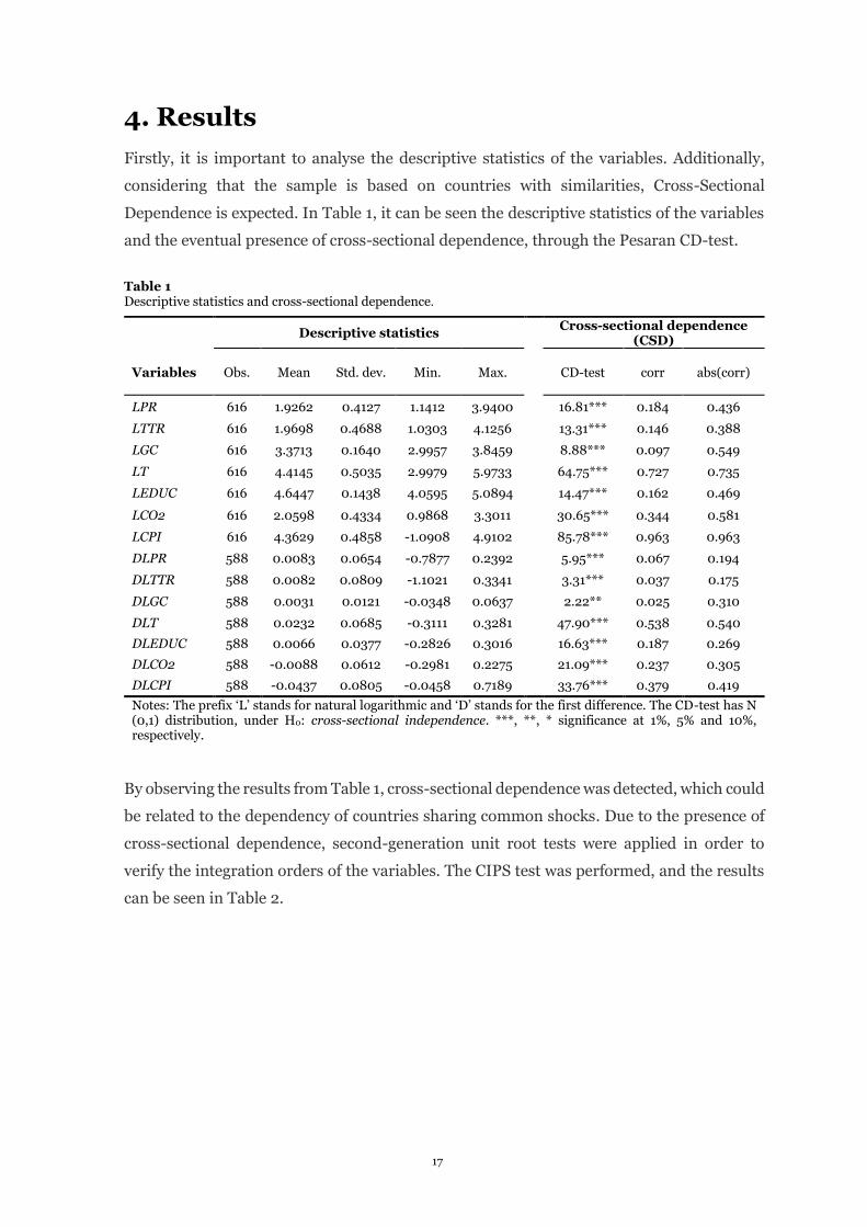
4. Results

Firstly, it is important to analyse the descriptive statistics of the variables. Additionally,

considering that the sample is based on countries with similarities, Cross-Sectional

Dependence is expected. In Table 1, it can be seen the descriptive statistics of the variables

and the eventual presence of cross-sectional dependence, through the Pesaran CD-test.

Table 1 Descriptive statistics and cross-sectional dependence.

By observing the results from Table 1, cross-sectional dependence was detected, which could

be related to the dependency of countries sharing common shocks. Due to the presence of

cross-sectional dependence, second-generation unit root tests were applied in order to

verify the integration orders of the variables. The CIPS test was performed, and the results

can be seen in Table 2.

Descriptive statistics Cross-sectional dependence

(CSD)

Variables

Obs.

Mean

Std. dev.

Min.

Max.

CD-test corr abs(corr)

LPR 616 1.9262 0.4127 1.1412 3.9400 16.81*** 0.184 0.436

LTTR 616 1.9698 0.4688 1.0303 4.1256 13.31*** 0.146 0.388

LGC 616 3.3713 0.1640 2.9957 3.8459 8.88*** 0.097 0.549

LT 616 4.4145 0.5035 2.9979 5.9733 64.75*** 0.727 0.735

LEDUC 616 4.6447 0.1438 4.0595 5.0894 14.47*** 0.162 0.469

LCO2 616 2.0598 0.4334 0.9868 3.3011 30.65*** 0.344 0.581

LCPI 616 4.3629 0.4858 -1.0908 4.9102 85.78*** 0.963 0.963

DLPR 588 0.0083 0.0654 -0.7877 0.2392 5.95*** 0.067 0.194

DLTTR 588 0.0082 0.0809 -1.1021 0.3341 3.31*** 0.037 0.175

DLGC 588 0.0031 0.0121 -0.0348 0.0637 2.22** 0.025 0.310

DLT 588 0.0232 0.0685 -0.3111 0.3281 47.90*** 0.538 0.540

DLEDUC 588 0.0066 0.0377 -0.2826 0.3016 16.63*** 0.187 0.269

DLCO2 588 -0.0088 0.0612 -0.2981 0.2275 21.09*** 0.237 0.305

DLCPI 588 -0.0437 0.0805 -0.0458 0.7189 33.76*** 0.379 0.419

Notes: The prefix ‘L’ stands for natural logarithmic and ‘D’ stands for the first difference. The CD-test has N (0,1) distribution, under H0: cross-sectional independence. ***, **, * significance at 1%, 5% and 10%, respectively.

18

Table 2 Second generation unit root tests.

Considering the null hypothesis for CIPS test is, series is I(1), by analysing the results, we

can conclude that all variables are either I(1) or I(0). As the variables are not I(2), the

posterior use of the ARDL model is shown to be appropriate. Due to the existence of cross-

sectional dependence in the variables, the Westerlund test of cointegration was also

computed for each model with constant. This test can only be performed with variables in

the same order of cointegration I(1). Using bootstrapping to obtain robust critical values,

the null hypothesis for this test is the non-existence of cointegration. The test results can be

seen in Table 3.

Table 3 Westerlund cointegration test.

By analysing the results, we can conclude that the null hypothesis was not rejected. This

demonstrates the absence of cointegration between variables. In order to test the adequacy

of RE against FE estimators, the Hausman test was performed. The Hausman test results,

as well as specification tests, can be observed in Table 4.

2nd generation panel unit root test CIPS

Variables Without trend With trend

LPR -4.566*** -3.938***

LTTR -2.903*** -1.910**

LGC -2.228** -1.811**

LT -1.848** 0.809

LEDUC -0.555 0.407

LCO2 1.307 -0.166

LCPI -8.332*** -1.016

DLPR -16.195*** -13.915***

DLTTR -15.815*** -13.482***

DLGC -3.270*** -0.103

DLT -5.964*** -3.570***

DLEDUC -6.429*** -5.664***

DLCO2 -8.996*** -8.630***

DLCPI -8.083*** -5.666***

Note: ***, **, * significance at 1%, 5% and 10%, respectively. H0: series is I (1).

Statistic Value Z-value Robust P-value

LPR LTTR LGC LPR LTTR LGC LPR LTTR LGC

Gt -1.837 -2.035 -0.815 -0.662 -1.685 4.618 0.071 0.020 0.884

Ga -2.067 -2.620 -1.057 4.866 4.398 5.721 0.510 0.124 0.958

Pt -6.339 -7.665 -4.509 0.480 -0.532 1.876 0.210 0.096 0.475

Pa -1.636 -1.851 -0.865 2.207 2.027 2.853 0.304 0.235 0.681

Note: the bootstrapping regression with 800 reps was performed; Gt and Ga test the cointegration of each country individually, and PT and Pa test the cointegration of the panel as a whole; the null hypothesis of the Westerlund cointegration test is no cointegration.

19

Table 4 Hausman and Specification tests.

The results confirm that the Fixed Effects model is the most suitable model for the three

measures of income inequality. The specification tests results show the rejection of the null

hypothesis for the modified Wald Test, demonstrating the presence of heteroscedasticity.

The presence of contemporaneous correlation for the 20/20 ratio model and absence for

Palma and Gini models. Finally, the results also show the rejection of the null hypothesis

for the Wooldridge test, proving that the data has first-order autocorrelation.

Succeeding the specification test results, the Driscoll and Kraay estimator was applied for

each model. The error structure for this estimator is assumed to be heteroskedastic,

autocorrelated and cross-sectional dependent. The OLS model, RE model, FE model and

FE model with robust standard errors were also estimated to control the heteroscedasticity.

The results for the Palma, 20/20 and Gini models can be observed and compared in Table

5, Table 6 and Table 7, respectively.

Table 5 Estimation Results for Palma model.

The results revealed that, in the short run, an increase of 1% in the DLCPI, decreases income

inequality by almost 27%. Meanwhile, in the long run, LCO2 is statistically significant,

where an increase of 1%, causes a decrease in income inequality by almost 4%. A higher

decrease of almost 7% on income inequality is caused by the 1% increase of LCPI.

Additionally, high levels of trade openness, in the short- or long-run, means higher levels of

Models DLPR DLTTR DLGC

Hausman test 102.05*** 114.43*** 77.82***

Modified Wald test 4049.25*** 1344.60*** 1250.34***

Pesaran test 1.631 2.619*** 0.288

Wooldridge test 57.746*** 76.141*** 64.222***

Note: ***, denote significance at 1%; The Hausman test tests null hypothesis as RE model is the preferred model; Modified Wald test, Pesaran test and Wooldridge test tests the null hypothesis of homoscedasticity, cross-sectional independence and no first-order autocorrelation, respectively.

Dependent Variable LPR OLS RE FE FE_robust FE D.K.

DLT 0.1874*** 0.1874*** 0.2242*** 0.2242** 0.2242**

DLEDUC -0.0005 -0.0005 -0.0117 -0.0117 -0.0117

DLCO2 -0.0222 -0.0222 -0.0383 -0.0383 -0.0383

DLCPI -0.1419* -0.1419* -0.2787*** -0.2787** -0.2787**

LPR -0.0347*** -0.0347*** -0.2915*** -0.2915*** -0.2915***

LT -0.0133** -0.0133** 0.1275*** 0.1275*** 0.1275***

LEDUC -0.0181 -0.0181 -0.0283 -0.0283 -0.0283

LCO2 0.0054 0.0054 -0.0425 -0.0425* -0.0425*

LCPI -0.0112 -0.0112 -0.0759*** -0.0759*** -0.0759***

Constant 0.2568** 0.2568** 0.5628** 0.5628** 0.5628***

Note: ***, **, * represent a significance level of 1%, 5% and 10%, respectively.

20

inequality. In fact, the increase of trade openness by 1% in a short and long run, causes an

increase in inequality of almost 22% and 12%, respectively. Besides the high significance of

the Error Correction Mechanism, the coefficient varies between -1 and 0. Thus

demonstrating that the model adjusts itself into equilibrium and confirms the existence of

a long-run relation statistically significant between the variables.

Table 6 Estimation Results for 20/20 model.

By analysing the results seen in Table 6, similarly to the Palma model, in the short- and

long-run, an increase of trade openness and consumer price causes an increase and decrease

of inequality, respectively. However, in this model, the results show that CO2 is statistically

significant in the short-run instead of a long run. In fact, an increase of 1% of DLCO2 causes

an increase of almost 8% in income inequality. The model also adjusts itself into equilibrium

with the coefficient of ECM highly significant and varying between -1 and 0.

Table 7 Estimation Results for Gini model.

The results shown in the models across the three tables demonstrate some similarities such

as consistency in signals and highly significant coefficient of the Error Correction

Mechanism. However, the results for the Gini model revealed less significance. In the short

run, an increase of 1% in the DLCO2 causes a decrease of almost 1% in income inequality.

Dependent Variable LTTR OLS RE FE FE_robust FE D.K.

DLT 0.2457*** 0.2457*** 0.3111*** 0.3111** 0.3111**

DLEDUC -0.0197 -0.0197 -0.0201 -0.0201 -0.0201

DLCO2 -0.0625 -0.0625 -0.0809 -0.0809* -0.0809**

DLCPI -0.1250 -0.1250 -0.3503*** -0.3503 -0.3503**

LTTR -0.0382*** -0.0382*** -0.3211*** -0.3211*** -0.3211***

LT -0.0178** -0.0178** 0.1664*** 0.1664*** 0.1664***

LEDUC -0.0219 -0.0219 -0.0557 -0.0557 -0.0557

LCO2 0.0086 0.0086 -0.0503 -0.0503 -0.0503

LCPI -0.0023 -0.0023 -0.0971*** -0.0971* -0.0971***

Constant 0.2548* 0.2548* 0.6991** 0.6991** 0.6991***

Note: ***, **, * represent a significance level of 1%, 5% and 10%, respectively.

Dependet Variable LGC OLS RE FE FE_robust FE D.K.

DLT 0.0008 -0.0021 0.0001 0.0001 0.0001

DLEDUC 0.0106 0.0097 0.0093 0.0093 0.0093

DLCO2 -0.0143* -0.0129* -0.0139* -0.0139 -0.0139*

DLCPI -0.0111 -0.0021 0.0078 0.0078 0.0078

LGC -0.0268*** -0.0398*** -0.1239*** -0.1239*** -0.1239***

LT -0.0015 -0.0033** 0.0017 0.0017 0.0017

LEDUC -0.0084** -0.0081 0.0022 0.0022 0.0022

LCO2 0.0000 -0.0012 -0.0111** -0.0111 -0.0111

LCPI -0.0051** -0.0043* -0.0039* -0.0039 -0.0039*

Constant 0.1614*** 0.2105*** 0.4426*** 0.4426*** 0.4426***

Note: ***, **, * represent a significance level of 1%, 5% and 10%, respectively.

21

While in the long run, an increase of 1% in the LCPI causes a decrease of less than 1% in

inequality. The main reason for this may be the lack of variation on the Gini variable. The

semi-elasticities and elasticities were also performed in order to assess the magnitude of the

effects. The results for the income inequality measures, Palma ratio, 20/20 ratio and Gini

coefficient are displayed in Table 8.

Table 8 Short-run impacts and elasticities.

One result deserves attention, the variable CPI have a negative effect in the short- and long-

run for all inequality models except on Gini in the short-run, where the variable is not

significant. The results also reveal that although the variable EDUC is not significant in any

model, trade has a positive effect in both the short- and long-run for the Palma and 20/20

ratios. Regarding the environmental variable, CO2 emissions, it has a negative effect in both

the short- and long-run on Gini approach. This negative effect is only seen also in the short-

run for the 20/20 ratio. This outcome will be discussed in the next section.

Models DLPR DLTTR DLGC

Short run-impactss (I) (II) (III) (IV) (V) (VI)

DLT 0.2242** 0.2280*** 0.3111** 0.3197** 0.0001

DLEDUC -0.0117 -0.0201 0.0093

DLCO2 -0.0383 -0.0809** -0.0684** -0.0139* -0.0153**

DLCPI -0.2787** -0.2796*** -0.3503** -0.3556** 0.0078

Elasticities

LT 0.4374*** 0.4786*** 0.5180*** 0.5578*** 0.0134

LEDUC -0.0969 -0.1735 0.0177

LCO2 -0.1459 -0.1567 -0.0897* -0.1002***

LCPI -0.2602*** -0.2773*** -0.3024*** -0.3287*** -0.0318* -0.0366***

Note: ***, **, * represent a significance level of 1%, 5% and 10%, respectively.

22

5. Discussion

As the results display trade openness coefficient positive in a short and long run, this

research supports the branch of the literature, which states that income inequality increases

with an increase in globalisation. Consistently with this branch of literature, such as Kanbur

(2015), when analysing the estimation results for Palma model, an increase of 1% in trade

openness causes an increase in income inequality of almost 22% in the short run and 12%

in the long run. Supporting this branch of literature, the estimation results for 20/20 model

suggest that an increase of 1% in trade openness in a short and long run, causes an increase

in inequality of almost 31% and 16%, respectively. Against the evidence shown in the work

of Kraay (2006), where openness to international trade is negatively correlated with the

Gini coefficient, the estimation results for the Gini model in this research display trade

openness as not significant in a short and long run. However, considering the other

estimation models such as Palma and 20/20 ratios, the results support trade openness as a

proxy of globalisation, a driver of income inequality for the OECD countries. To Stiglitz

(1998), a reason for this may be due to disparities in returns to education and skills. The

results shown in this research contradict the work of Asteriou et al. (2014), where evidence

suggests a reduction in inequality from trade openness in the 27 countries in the European

Union. This contradiction might be due to factors related to the methodology and time span

used or even variables chosen as globalisation proxies. Whereas the previous study defends

that policies to mitigate inequality should be in regards to foreign direct investment, our

research suggests that should be in regards to trade openness.

Regarding the impact of the climate change on income inequality, the results show that an

increase of 1% in carbon dioxide emissions causes a decrease in the inequality of almost 8%

in a short run and 4% in the long run. This result is shown in the 20/20 and Palma

estimation models, respectively. Supporting the decrease in inequality by the increase of 1%

in carbon dioxide emissions in the short run, the estimation results for the Gini model,

display a decrease in inequality by almost 1%. This research contradicts the evidence shown

in the work of Grunewald et al. (2017), which the main findings reveal that reduction in

income inequality for upper-middle-income and high-income economies will

simultaneously cause carbon dioxide emissions to decrease. The reason for this

contradiction might be due to the data set used, covering 158 countries with annual

measurements from 1980 to 2008, being associated with one of the most extensive data sets

in the existing literature on the relationship between income inequality and carbon

emissions. Overall, this research finds that an increase in carbon dioxide emissions per

capita causes a decrease in income inequality in a short and long run, for the OECD

countries. Supporting the work of Ravallion et al. (2000), this outcome implies that there is

23

a trade-off between inequality and emissions. In order to decrease income inequality, there

is a need to increase carbon dioxide emissions per capita. Then policymakers will be

challenged to find effective policies.

Considering the estimation results for the income inequality measures models, the results

reveal the importance of fiscal and monetary policies such as consumer price index.

Through cross-validation, the results suggest that an increase in the consumer price index

causes a decrease in income inequality in the short and long run for the OECD countries.

When analysing the estimation results for the Palma, 20/20 and Gini model in a short and

long run, the consumer price index coefficient displays as negative with the exception of

Gini model in the long run, which does not display statistical significance. This outcome

contradicts the work of Cysne et al. (2005), which demonstrates a formal link between

inflation and income inequality, as an increase in inflation leads to a deterioration of the

income distribution.

As stated before, there still is a lack of consensus on determining measures for inequality.

This lack of consensus is due to limitations in the models in which should be taken into

account when interpreting conclusions or making decisions based on inequality measures.

For instance, inequalities with distinct meanings may correspond to the same index value

in the Gini coefficient (Pascoal and Rocha, 2018). The main limitation for the Palma and

20/20 ratios is that, as partial measures, the ratios do not account for full distribution.

Therefore, although the Gini coefficient is the standard measure of income inequality, the

study of other measures simultaneously, allows for more robustness and consistency in the

results. The battery of tests performed in this study reveals that of the three income

inequality measures analysed, the 20/20 ratio is the most suitable for the data set used.

However, the study of the Palma ratio and Gini coefficient allowed consistency and

validation in the results and revealed relevant findings such as the increase of carbon

dioxide emissions causes a decrease in income inequality in the long run for the OECD

countries.

Overall, the results in this study suggest that for the Organisation for Economic co-

operation and development, policymakers should take in consideration policies to decrease

trade openness to mitigate inequality. Additionally, in order to achieve growth equality in

upper-middle-income and high-income economies, policies should be considered regarding

the gradual increase of carbon dioxide emissions and inflation for the observed countries.

24

6. Conclusion

The main objective of this study is to estimate the degree of globalisation impact on income

inequality in the short and long run for the countries members of the Organisation for

Economic Co-operation and Development, covering the time span from 1993 to 2014.

Additionally, inequality measures and other drivers in the short and long run were also

studied.

This study contributes to the literature describing which factors have an impact on income

inequality using an econometric approach. The data set was subjected to an exhaustive

battery of tests to analyse the properties of the data series and guarantee that the most

suitable estimator was used. Through the Driscoll-Kraay with fixed effects estimator and

the Autoregressive Distributed Lag approach to determine the effects in the short and long

run, the overall results of this investigation reveal high consistency with both the literature

and the economic theory. The main findings suggest important policy implications to reduce

income inequality. For instance, as the results suggest that an increase of trade openness

causes an increase of income inequality, it might indicate that greater mobility of goods,

capital and labour, pressures the freedom of governments to mitigate inequality through

redistributive instruments. Therefore, trade policies should consider the implementation of

redistributive systems, such as Conditional Cash Transfers. As the increase of consumer

price index causes a decrease in income inequality, the countries members of OECD should

maintain the control of inflation levels, through central banks. In regards to climate change,

policies should consider the trade-off between income inequality and dioxide carbon

emissions. A policy that could successfully address this trade-off is a revenue-neutral

redistributive carbon tax that would encourage the reduction of emissions while the

revenues could be redistributed to improve public services used by low-income households.

For future research, besides trade openness, it can be considered the multidimensional

globalisation characteristic and study social and political characteristics. The study of low

and middle-income economies should also be considered when increasing the sample size

in order to compare disparities in income levels. For more consistency and robustness,

future investigations should include several inequality measures and not only the standard

measure of income inequality, the Gini Coefficient.

25

References

Albanesi, S. (2007). Inflation and inequality. Journal of Monetary Economics, 54(4),

1088–1114. https://doi.org/10.1016/j.jmoneco.2006.02.009

Arellano, M., & Bond, S. (1991). Some Tests of Specification for Panel Data: Monte Carlo

Evidence and an Application to Employment Equations. The Review of Economic Studies,

58(2), 277. https://doi.org/10.2307/2297968

Asteriou, D., Dimelis, S., & Moudatsou, A. (2014). Globalization and income inequality: A

panel data econometric approach for the EU27 countries. Economic Modelling, 36, 592–

599. https://doi.org/10.1016/j.econmod.2013.09.051

Berg, A. G., & Ostry, J. D. (2017). Inequality and Unsustainable Growth: Two Sides of the

Same Coin? IMF Economic Review, 65(4), 792–815. https://doi.org/10.1057/s41308-017-

0030-8

Bourguignon, F., & Morrisson, C. (2002). Inequality among world citizens. The American

Economic Review, 92(4), 727–744.

Breunig, R., & Majeed, O. (2020). Inequality, poverty and economic growth. International

Economics, 161, 83–99. https://doi.org/10.1016/j.inteco.2019.11.005

Bumann, S., & Lensink, R. (2016). Capital account liberalization and income inequality.

Journal of International Money and Finance, 61, 143–162.

https://doi.org/10.1016/j.jimonfin.2015.10.004

Charles-coll, J. a. (2011). Understanding Income Inequality : Concept , Causes and

Measurement. International Journal of Economics and Management Sciences, 1(3), 17–

28.

Chiquiar, D. (2008). Globalization, regional wage differentials and the Stolper-Samuelson

Theorem: Evidence from Mexico. Journal of International Economics, 74(1), 70–93.

https://doi.org/10.1016/j.jinteco.2007.05.009

Cobham, A., & Sumner, A. (2013). Is It All About the Tails? The Palma Measure of Income

Inequality. Center for Global Development Working Paper, 2013(September 2013), 1–42.

https://doi.org/10.23.13

Cysne, R. P., Maldonado, W. L., & Monteiro, P. K. (2005). Inflation and income inequality:

A shopping-time approach. Journal of Development Economics, 78(2), 516–528.

26

https://doi.org/10.1016/j.jdeveco.2004.09.002

Dabla-Norris, E., Kochhar, K., Suphaphiphat, N., Ricka, F., & Tsounta, E. (2015). Causes

and Consequences of Income Inequality: A Global Perspective. Staff Discussion Notes,

15(13), 1. https://doi.org/10.5089/9781513555188.006

de Haan, J., & Sturm, J. E. (2017). Finance and income inequality: A review and new

evidence. European Journal of Political Economy, 50(C), 171–195.

https://doi.org/10.1016/j.ejpoleco.2017.04.007

Dalton, H. (1920). The Measurement of the Inequality of Incomes. The Economic Journal,

30(119), 348–361.

Dollar D, & Kraay A. (2001). Trade, Growth and Poverty Development Research Group,

World Policy Research

Dreher, A. (2006). Does globalization affect growth? Evidence from a new index of

globalization. Applied Economics, 38(10), 1091–1110.

https://doi.org/10.1080/00036840500392078

Driscoll, J. C., & Kraay, A. C. (1998). Consistent covariance matrix estimation with spatially

dependent panel data. Review of Economics and Statistics, 80(4), 549–559.

https://doi.org/10.1162/003465398557825

Easterly, W., & Fisher, S. (2001). Inflation and the Poor. Journal of Money, Credit and

Banking, Vol. 33, No. 2, pp1. 160-178

Erosa, A., & Ventura, G. (2002). On inflation as a regressive consumption tax. Journal of

Monetary Economics, 49(4), 761–795. https://doi.org/10.1016/S0304-3932(02)00115-0

Frank, M. W. (2009). Inequality and growth in the united states: Evidence from a new state-

level panel of income inequality measures. Economic Inquiry, 47(1), 55–68.

https://doi.org/10.1111/j.1465-7295.2008.00122.x

Frankel, J. A., & Romer, D. (1999). Does trade cause growth? American Economic Review,

89(3), 379–399. https://doi.org/10.1257/aer.89.3.379

Furceri, D., & Loungani, P. (2015). Capital Account Liberalization and Inequality. IMF

Working Papers, 15(243), 1. https://doi.org/10.5089/9781513531083.001

Goldin, C., & Katz, L. (2007). Long-Run Changes in the US Wage Structure: Narrowing,

27

Widening, Polarizing. National Bureau of Economic Research.

http://www.nber.org/papers/w13568

Grossman, G. M., & Helpman, E. (2015). Globalization and growth. American Economic

Review, 105(5), 100–104. https://doi.org/10.1257/aer.p20151068

Grunewald, N., Klasen, S., Martínez-Zarzoso, I., & Muris, C. (2017). The Trade-off Between

Income Inequality and Carbon Dioxide Emissions. Ecological Economics, 142, 249–256.

https://doi.org/10.1016/j.ecolecon.2017.06.034

Gurgul, H., & Lach, Ł. (2014). Globalization and economic growth: Evidence from two

decades of transition in CEE. Economic Modelling, 36, 99–107.

https://doi.org/10.1016/j.econmod.2013.09.022

Hamori, S., & Hashiguchi, Y. (2012). The effect of financial deepening on inequality: Some

international evidence. Journal of Asian Economics, 23(4), 353–359.

https://doi.org/10.1016/j.asieco.2011.12.001

Hausman, J. A. (1978). Specification Tests in Econometrics. Econometrica, 46(46), 1251–

1271.

Hoechle, D. (2007). Robust standard errors for panel regressions with cross-sectional

dependence. Stata Journal, 7(3), 281–312. https://doi.org/10.1177/1536867x0700700301

Hsiao, C. (2007). Panel data analysis-advantages and challenges. Test, 16(1), 1–22.

https://doi.org/10.1007/s11749-007-0046-x

Hübler, M. (2017). The inequality-emissions nexus in the context of trade and development:

A quantile regression approach. Ecological Economics, 134, 174–185.

https://doi.org/10.1016/j.ecolecon.2016.12.015

Jauch, S., & Watzka, S. (2016). Financial development and income inequality: a panel data

approach. Empirical Economics, 51(1), 291–314. https://doi.org/10.1007/s00181-015-

1008-x

Kanbur, R. (2015). Globalization and inequality. In Handbook of Income Distribution (1st

ed., Vol. 2). Elsevier B.V. https://doi.org/10.1016/B978-0-444-59429-7.00021-2

Keohane, R. O., & Nye, J. N. (2000). What's New? What's Not? (And So What?). Foreign

Policy, No. 118, pp. 104-119

28

Kim, D. H., & Lin, S. C. (2011). Nonlinearity in the financial development-income inequality

nexus. Journal of Comparative Economics, 39(3), 310–325.

https://doi.org/10.1016/j.jce.2011.07.002

Kraay, A. (2006). When is growth pro-poor? Evidence from a panel of countries. Journal of

Development Economics, 80(1), 198–227. https://doi.org/10.1016/j.jdeveco.2005.02.004

Kuznets, S. (1955). Economic Growth and income inequality. American Economic Review,

45(1), 1–28. https://doi.org/10.1257/aer.99.1.i

Lin, S. C., (River) Huang, H. C., & Weng, H. W. (2006). A semi-parametric partially linear

investigation of the Kuznets’ hypothesis. Journal of Comparative Economics, 34(3), 634–

647. https://doi.org/10.1016/j.jce.2006.06.002

Liu, C., Jiang, Y., & Xie, R. (2019). Does income inequality facilitate carbon emission

reduction in the US? Journal of Cleaner Production, 217, 380–387.

https://doi.org/10.1016/j.jclepro.2019.01.242

Marjit, S., & Acharyya, R. (2003). The Standard Trade Theory: How far Does it Go? 37–

51. https://doi.org/10.1007/978-3-642-57422-1_3

Marques, L. M., Fuinhas, J. A., & Marques, A. C. (2017). Augmented energy-growth nexus:

Economic, political and social globalization impacts. Energy Procedia, 136, 97–101.

https://doi.org/10.1016/j.egypro.2017.10.293

Milanovic, B. (2011). A short history of global inequality: The past two centuries.

Explorations in Economic History, 48(4), 494–506.

https://doi.org/10.1016/j.eeh.2011.05.001

Milanovic, B. (2013). Global Income Inequality By the Numbers: In History and Now. HSE

Publishing House

Milanovic, B., & Lakner, C. (2013). Global Income Distribution Dynamics Dataset.

December, 68.

Milanovic, B., Lindert, P. H., & Williamson, J. G. (2011). Pre-Industrial Inequality.

Economic Journal, 121(551), 255–272. https://doi.org/10.1111/j.1468-0297.2010.02403.x

Ostry, J., Berg, A., & Tsangarides, C. (2014). Redistribution, Inequality, and Growth. Staff

Discussion Notes, 14(02), 1. https://doi.org/10.5089/9781484352076.006

29

Palma, J. G. (2006). Globalizing inequality: “centrifugal” and “centripetal” forces at work.

DESA Working Paper, 35, 1–26.

Palma, J. G. (2011). Homogeneous Middles vs. Heterogeneous Tails, and the End of the

“Inverted-U”: It’s All About the Share of the Rich. Development and Change, 42(1), 87–153.

https://doi.org/10.1111/j.1467-7660.2011.01694.x

Partridge, M. D. (1997). Is Inequality Harmful for Growth? The American Economic

Review, Vol. 87, N0. 5, pp. 1919-1032

Partridge, M. D. (2005). Does income distribution affect U.S. State economic growth.

Journal of Regional Science, 45(2), 363–394. https://doi.org/10.1111/j.0022-

4146.2005.00375.x

Pascoal, R., & Rocha, H. (2018). Inequality measures for wealth distribution: Population vs

individuals perspective. Physica A: Statistical Mechanics and Its Applications, 492, 1317–

1326. https://doi.org/10.1016/j.physa.2017.11.059

Pesaran, M. H. (2004). General Diagnostic tests for Cross Section dependence in

Panels:Cambridge working Paper in Economics. IZA Discussion Paper, 1240.

Pesaran, M. H. (2007). A Simple Panel Unit Root Test In The Presence Of Cross Section

Dependence. Journal of Applied Econometrics, 22(2), 265–312.

Pigou, A. C. (1920). The economics of welfare. The Economics of Welfare, 1–876.

Ravallion, M. (2000). Carbon emissions and income inequality. Oxford Economic Papers,

52(4), 651–669. https://doi.org/10.1093/oep/52.4.651

Sherif Khalifa, & Sherine El Hag. (2010). Income Disparities, Economic Growth, and

Development As a Threshold. Journal of Economic Development, 35(2), 23–36.

https://doi.org/10.35866/caujed.2010.35.2.002

Solt, F. (2016). The Standardized World Income Inequality Database*. Social Science

Quarterly, 97(5), 1267–1281. https://doi.org/10.1111/ssqu.12295

Stiglitz, J. E. (1998). More Instruments and Broader Goals: Moving toward the Post-

Washington Consensus, World Institute for Development Economics Research

Westerlund, J. (2007). Testing for error correction in panel data. Oxford Bulletin of

Economics and Statistics, 69(6), 709–748. https://doi.org/10.1111/j.1468-

30

0084.2007.00477.x

Wooldridge, J.M (2002). Econometric Analysis of Cross Section and Panel Data