MPRAMunich Personal RePEc Archive

Competition and Economic Growth: anEmpirical Analysis for a Panel of 20OECD Countries

Alessandro Diego Scopelliti

University of Warwick, Department of Economics

December 2009

Online at http://mpra.ub.uni-muenchen.de/20127/MPRA Paper No. 20127, posted 19. January 2010 00:17 UTC

1

Competition and Economic Growth:

an Empirical Analysis for a Panel of 20 OECD Countries

Alessandro Diego Scopelliti*§

Abstract

This paper aims at analyzing, from an empirical point of view, the relationship between product

market competition and economic growth, using the data on multi-factor productivity for a panel of 20

OECD countries over a period 1995-2005, and considering the role of the distance from the technological

frontier in the growth process.

|Section A examines the impact of economic freedom and of the distance to frontier on the level and

on the growth rate of multi-factor productivity. The analysis distinguishes between the indicators of business

freedom and trade freedom, as proxies for the competitive pressures coming from domestic market and from

foreign market. Then, trade liberalizations are more beneficial for the countries far from the frontier, because

they can exploit the opportunities given by international trade also in order to adopt the existing technologies

developed by the advanced economies. On the other hand, business liberalizations are more advantageous for

the countries close to the frontier, because the elimination of regulatory barriers increases the possibility of

entry in the market and then rises the potential competition to the incumbent firms.

Section B studies the effect of product market regulation, employment protection legislation and of

the distance to frontier on the level and on the growth rate of multi-factor productivity. Product market

liberalization as well as labour market deregulation determine an increase of total factor productivity:

moreover, the interaction of market rigidities with the distance to the frontier mostly displays an innovation-

enhancing effect, since the positive effect of market liberalizations on TFP is higher for the countries close to

the frontier, where the existing technology level would reinforce the incentive for innovation.

JEL Classification: L43, L44, O43, O47

Keywords: multi-factor productivity, economic freedom, product market regulation, employment protection

legislation, distance to frontier

________________________________________________________________________________________________* University of Warwick and University of Catania. Corresponding address: Department of Economics, University ofWarwick, CV4 7AL Coventry, United Kingdom. E-mail: A.D.Scopelliti@warwick.ac.uk§ I am particularly grateful to Ilde Rizzo for her precious and stimulating supervision. I am indebted with JacquesMairesse and Jimmy Lopez for providing some of the data used in the empirical analysis and for interesting discussionson the results. I am grateful to Francesco Forte for useful suggestions and for insightful observations. I also thankPhilippe Askenazy, Fabrizio Coricelli and Massimiliano Ferrara for helpful comments. All the errors are mine.

2

1.1 Introduction

This paper presents an empirical analysis of the relationship between product market

competition and economic growth for a panel of OECD countries: in particular it wants to study

whether specific policies aimed at improving product market competition have a positive or

negative impact on productivity growth, in order to derive some indications about the design of

competition policy in a growth-enhancing perspective. Clearly, this topic assumes a specific

relevance for the case of Europe, because of the productivity slowdown occurred in the last fifteen

years with respect to USA. While the European Union registered a growth rate of total factor

productivity always higher than the United States during the second post-war period, from the

second half of nineties it has recorded a growth rate of total factor productivity lower than the USA.

This is frequently explained by the lack of structural reforms for product and labour markets in the

European Union with respect to the United States. For this reason, it can be interesting to verify

whether product market reforms expected to increase the degree of competition can raise the growth

rate of productivity, as well as to observe whether policies aimed at reducing both product and

labour market rigidities may improve the growth performance of an economy.

The empirical literature about the relation between product market competition and

economic growth has shown an important development in the last few years for two reasons: firstly,

because the elaboration of new models of endogenous growth has induced the need of an empirical

verification of the new theoretical predictions: secondly, because the political debate on the most

appropriate economic policies for sustaining long-run growth also requires some indications

regarding the impact of liberalization policies and deregulation reforms on the growth rate of total

factor productivity.

In general, the empirical estimation of the relationship between competition and growth

presents some technical issues that have not been completely solved in the existing empirical

literature on the topic. For this reason it is worth to examine the main problems occurred in these

studies and to consider some of the adopted solutions before exposing the empirical analysis

presented in the next chapter. In particular, we will consider two aspects. The first element is the

difficulty to introduce in the empirical analysis a specification correspondent to the results of the

theoretical models previously discussed, with reference to the identification of the relevant

variables: this limits the concrete possibility to empirically test the conclusions coming from the

existing and diverging theoretical models. In general, the issue regards both the dependent variable

and the explanatory variable, but it is more difficult to be solved for the second one. A second

aspect worth to be considered is the opportunity to introduce, for the explanatory variable, an

interaction term regarding the distance from technological frontier, in order to study whether and

3

how the impact of competition on growth may change depending on the technological gap between

the observed country or industry and the country or industry which is the technological leader, as

suggested by a recent literature on endogenous growth.

Then, a key issue in the empirical analysis of the relationship between competition and

growth is the identification of the explanatory variable, since it is necessary to choose some

measures of product market competition which can proxy the variables used in the theoretical

models. For this reason, the following empirical analysis is divided in two sections: in the first one,

market competition is proxied by some measures of economic freedom, and in particular of

business freedom and trade freedom; in the second one, the relevant variable is the index of product

market regulation, computed by OECD for non-manufacturing industries and moreover we explore

the hypothesis of an interaction between product and labour market rigidities. After the presentation

of these two analyses, in the last section we provide a comparison of the main results obtained for

each study, both in order to draw some considerations about the choice of the explanatory variable,

and in order to develop some conclusions about the implementation of various growth-enhancing

policies.

1.2 The identification of the dependent variable

In the existing literature, the dependent variable of the model (the growth rate of the

economy) is generally defined by the growth rate of total factor productivity, which is also preferred

to the growth rate of GDP. The choice is clearly explained by the purposes of the study. In

particular, we are interested in analyzing how competition can affect, through the incentives for

innovation, the main source of economic growth, which is technological progress. Then, in this

perspective, the total amount of inputs employed in the production process is not relevant and the

variations of the quantity of capital and labour should not be considered. For this reason the growth

of total factor productivity, which includes any output growth which is not determined by an

increase of production inputs, is an appropriate indicator for the improvements in the state of

technology. Of course, the estimates of TFP growth, since they depend on the computation of a

residual growth rate after considering the variation of inputs, are not univocally definite but they

may change according to the weights assigned to each production input (capital or labour) in

evaluating the relative contribution to the growth rate of GDP.

Another solution for the dependent variable, proposed by some studies focused on the

relation between competition and innovation, is to use some measures of innovative output, such as

patenting activity or innovation counts. In general, a measure of patenting can be an adequate

choice for the dependent variable, given that the patent is the main instrument provided by

4

intellectual property law in order to protect the final result of an innovative activity. But two main

objections must be considered.

The first one is about the heterogeneity of patents: they have very different values depending

on the potential usage of the patented idea, then a merely quantitative indicator of the number of

patents would not be an appropriate solution. For this reason, some studies (Aghion, Bloom,

Blundell, Griffith and Howitt, 2005) propose as dependent variable a measure of citation-weighted

patents. Given that the value of a patent depends on the exploitation of its knowledge content for

further innovative output, the importance of each patent is weighted according to the number of

times it is cited by other patents. This approach also allows to take into consideration the knowledge

spillovers coming from innovative activity: this is quite important for theoretical reasons, given that

the positive externalities due to the diffusion of new ideas are key elements in the endogenous

growth literature in order to explain the overcoming of the issue of decreasing marginal returns to

capital.

The second objection concerns the incomplete diffusion of the patent as a means for

protecting intellectual property: while patents are very common in some sectors (such as

pharmaceuticals), they are relatively rare in other industries (for example in software industry). This

observation is very relevant because it discourages the usage of patenting counts as measures of

innovative output: it wouldn’t make sense to employ an indicator which is adequate only for some

industries but not for other ones. For example, a very important antitrust case on innovation activity

and intellectual property, such as the Microsoft case, doesn’t present any patenting issue, given that

the exclusive exploitation of this innovation depends on the secrecy of the source codes employed

by the software1.

These observations show that a measure of patenting activity cannot be a good dependent

variable for the model and that TFP growth must be preferred to it. Of course, this doesn’t exclude

the possibility to employ an indicator of patenting activity as a control variable in the empirical

analysis, given that patent protection, even only for some industries, is an important incentive for

inducing investments in R&D and then for promoting innovation. So it is reasonable to assume that

TFP growth is positively correlated to patenting measures, since patents contribute to the advance

of technological progress.

1 Indeed, as described in the previous chapter, the key point of the dispute between Microsoft and the European

Commission regarded the possibility for the competitors to know the interface information of Microsoft Windows in

order to guarantee the interoperability between the operating systems for personal computers and the operating systems

for workgroup servers.

5

1.3 The identification of the explanatory variable: product market competition

On the opposite, many issues regard the identification of one (or more than one) adequate

proxy for the explanatory variable, because of the difficulty to measure the degree of product

market competition. Most theoretical models use the Lerner index as an indicator of market power

and then the inverse of Lerner index as a measure of competition. But this index cannot be used in

the empirical analysis, neither at a firm-level, nor at an aggregate level, because of the possible

endogeneity of the regressor with respect to the dependent variable. In particular, Aghion, Blundell,

Griffith, Howitt and Van Reenen (2005), studying the relation between competition and innovation

at a firm level, measure the Lerner index as the following ratio:

turnover

tcosfinancialprofitsoperatingLI

But, as it is correctly observed, this measure of Lerner index, depending on the turnover and

on the operating profits of a firm, shows a problem of endogeneity, because there is a possible

reverse causality between the multi-factor productivity of a firm and its profit margin. In fact, the

firms with a higher productivity may increase their profit margins, either because they expand their

market share and market power with respect to other firms of the same industry, or because they

exploit the economies of scale coming from an increase of the amount of output produced. Then it

is necessary to verify the possibility to use other existent measures of competition or, if it is not

possible, to define the appropriate econometric technique in order to solve the endogeneity problem

of the Lerner Index.

For example, other possible measures of competition proposed in the IO literature are

market share, Herfindhal index, concentration ratio, firm size. But these indicators of market

structure necessarily require a previous definition of the geographic and product market, given that

they can be determined only with reference to a given specific context. After defining the market, it

is possible to identify the firms operating in that market and then compute the market share of each

firm, as well as the Herfindhal index for the industry and the concentration ratio for the firms with

the largest market share. In this perspective, market definition is fundamental for determining the

degree of competition existent in a particular market: indeed, once defined the market structure, a

related indicator of product market competition is computed in order to explain, as a final objective,

how competitive pressures influence the incentives of firms for innovation.

But this approach for market definition may imply some difficulties due to firm

heterogeneity, especially for firms belonging to the same industry and supplying the same product.

For example, some firms of an industry may operate in international markets, while other firms may

sell only in domestic markets. In this case, different market definitions may imply diverse results

6

for the measure of product market competition, depending on whether or not the reference market is

defined as a domestic one or as an international one2.

On the basis of these observations, it is clear that a priori market definition may determine

erroneous results for the individuation and the computation of some related indicators of market

structure, such as market share, concentration ratio or Herfindhal index. As a consequence, it is not

appropriate to employ these measures of product market competition for the analysis of the relation

between competition and growth. Moreover, another argument against this choice is due to the fact

that the measures of market structure previously proposed are not always monotonic with respect to

the degree of competition (Boone, 2000). On the contrary, the Lerner index doesn’t imply this

problem.

Then, it is necessary to use the method of the instrumental variables in order to obtain a

measure of competition, correlated with the economic rents obtained by firms, which produces

effects on total factor productivity through an indirect way (that is via the impact on profit margin),

without being influenced by TFP.

1.3.1 The identification of the explanatory variable: economic freedom

In some empirical literature, when it is not possible to use the inverse of Lerner Index as an

explanatory variable for the discussed endogeneity problem, product market competition is

instrumented by measures of economic freedom, as computed by different organizations or

foundations. In general, these measures of economic freedom, which are defined on the basis both

of qualitative judgements and of statistical data, are not correlated to the dependent variable (the

growth rate of TFP). This means that economic freedom can influence the growth rate of TFP but is

not affected by it. Given the importance of this assumption for the choice of the instrumental

variable, it is worth to discuss the possible objections to the reliability of the hypothesis.

A political economy consideration (Pitlik, 2008) suggests the existence of a possible causal

relationship between growth and liberalizations, because the macroeconomic performance (even

2On the contrary, this problem doesn’t apply for the definition of the relevant market, as it is usually employed

in competition policy analysis, in order to identify the economic context where to evaluate the behaviour of specific

firms. As described in the previous chapter for the abuse of dominance, the implementation of competition policy

involves a case-by-case definition of the relevant market, given that antitrust authorities must examine the conduct of

single firms in order to verify whether a collusive agreement or a dominant position may compromise competition. The

definition assumes the analysis of the supplied product and the individuation of the substitute goods and it is aimed at

individuating the set of possible competitors for the firm. This evaluation is determinant for the final judgement about

the competitive or anticompetitive nature of the activity of a firm, but it is anyway proposed for a specific firm and then

it allows to take into account the peculiarities of each undertaking.

7

conditioned to the type of political regime) can have an impact on liberalization processes, either by

increasing their opportunity during a recession, or by making them more difficult (also because less

urgent) during a boom. As a consequence, the indicator of economic freedom could be endogenous

with respect to the growth rate of the economy.

Anyway, this is not enough for excluding the use of economic freedom as an exogenous

regressor. In fact, this reasoning essentially takes into account a short-run macroeconomic

performance, as explained by the growth rate of GDP. On the opposite, the effects we are interested

in, regarding the causal relationship between competition and growth, are related to a long-run

macroeconomic performance, as determined by the growth rate of total factor productivity. Today’s

market structure, influencing the incentives for innovation, produces its effects on long-run growth,

and then the ex ante determinants of liberalization processes should not be relevant from this point

of view.

Nevertheless, the usage of economic freedom indexes may however induce some misleading

results, depending on the way they are prepared. In fact, these indicators frequently collect many

different aspects (business freedom, trade freedom, financial freedom, freedom from corruption,

property rights enforcement, government size), which identify a dimension larger than (and then

different from) product market competition.

However, the broad and eclectic coverage of the economic freedom indicator is not a

determinant point against the employment of this index: in fact, when the method of instrumental

variables is implemented, through the technique of two-stage least squares, the chosen instrument

must be something different from the variable of interest. So, the generality of the economic

freedom index is not a problem unless it questions the key elements of a good instrumental variable:

the correlation with the variable of interest; the absence of a direct correlation with the dependent

variable, but only an indirect correlation through the variable of interest. About the first

requirement, the correlation between competition and economic freedom is clearly shown in the

studies which follow this strategy (Griffith and Harrison, 2004): a country with a higher degree of

product market competition also enjoys a greater economic freedom. But, regarding the second

aspect, a problem can arise if, due to the various components included in the computation of the

economic freedom index, some of them are correlated to the growth rate of the economy, for

example because an economy growing faster may better promote the degree of financial

development.

For this reason, in principle, the specific indicators of economic freedom could be more

appropriate than the general index, because they are more directly related to the variable of interest.

But the practical use of the individual indicators can give meaningless results in statistical terms,

especially when the index is defined on the basis of a qualitative judgement, formulated in a

8

comparative way with respect to the situation of other countries. In those cases, since the relative

position of each country in the rankings of a specific aspect of economic freedom is frequently

unchanged, this sometimes implies the assignment of the same score, notwithstanding the

improvements occurred over time. As a consequence, the coefficient of a specific indicator of

economic freedom may result not statistically significant, especially with reference to the within

variation, simply because of the scarce quality of the data.

Finally, the indicators of economic freedom show an advantage, because they have been

collected for a large number of countries and also for a significant time series, so they can be

usefully employed, in a dynamic efficiency perspective, for an analysis of the determinants of total

factor productivity. On the contrary, very few indices of product market competition, differentiated

by country and over a time series, are available in order to be employed for a dynamic analysis.

1.3.2 The identification of the explanatory variable: product market regulation

An alternative way to measure product market competition is to observe the market rigidities

that can negatively affect the degree of competition in the marketplace. For this purpose, various

market rigidities can be taken into consideration, such as the barriers to entry or to exit, the vertical

integration of an industry, the presence of public ownership, the pricing of a natural monopoly, the

existence of collusionary agreements or the dominance of a firm in the market structure. All these

market rigidities can limit competition in different ways: for example, the vertical integration of a

given industry may produce some foreclosure effect on the other possible competitors; the barriers

to entry exclude the potential competition coming from new entrants; the existence of a strong

component of public ownership may reduce the initiative of private firms; the pricing of a natural

monopoly can impose a welfare loss for consumers. In order to have a broad overview of the

obstacles for perfect competition in the marketplace, we can summarize all these aspects of market

rigidities in a general concept of product market regulation, which can be considered as an inverse

of product market competition.

Some indicators of product market regulation have been elaborated by the OECD in the last

few years: so they can be used in order to define, from the negative point of view, the degree of

product market competition in an economy or in an industry. In particular, an economy-wide

indicator of product market regulation, called PMR, has been computed by the OECD for 1998,

2003 and 2008 and it is employed in the study by Nicoletti and Scarpetta (2003); but the

unavailability of such index for a significant time series doesn’t allow to implement it in order to

observe properly the long-run effects on economic growth.

9

From this point of view, a better solution is given by the industry-specific indicators of

product market regulation, also elaborated by the OECD but only for some non-manufacturing

industries: in particular, we can consider the index of product market regulation for Energy,

Transport and Communication sectors, named ETCR. This is available for a time period between

1975 and 2003 and collects the data for seven industries, that is electricity, gas, airlines, rail, road

freight, post and telecoms. This index provides a sufficiently long time series in order to observe the

effect of regulation on productivity growth and in fact it has been employed in some recent studies,

such as the paper by Aghion, Askenazy, Bourlès, Cette and Dromel (2009). But it is referred just to

some networks industries and then it cannot be considered as an appropriate indicator for the whole

economy.

However, this doesn’t exclude that the regulation in the observed network industries can

have indirect effects on the whole economy, simply because the firms involved in such non-

manufacturing industries supply some intermediate goods or services which are used as inputs for

production in the final sector of the economy. This observation is perfectly consistent with the two-

sector structure of the economy in endogenous growth models, where we usually assume perfect

competition in the final sector and market imperfections in the intermediate sector. So this implies

that an empirical analysis using such indicator for product market regulation can capture not only

the direct impact of regulation in energy, transport and communication sectors, but also the indirect

effect of regulation on the whole economy.

Moreover, this idea about the indirect impact of the regulation in intermediate industries on

the whole economy has been exploited for the construction of another indicator of product market

regulation, called as regulation impact (RI). More precisely, the indices of regulation impact are

sectoral indicators that measure the “knock-on” effects of the regulation in non-manufacturing

sectors on all the sectors of the economy. Of course, this impact depend on the extent of the anti-

competitive regulation in non-manufacturing sectors as well as on the importance of these sectors as

suppliers of intermediate inputs for the final sector. Then, for a given final sector k, the regulation

impact in time t is computed as follows:

jkj

jtkt wNMRRI

So the indicator RIkt is a weighted sum of the indices of anti-competitive regulations, as they are

observed in each non manufacturing sector j supplying some inputs for the production process. The

weight wjk measures the total input requirement of final sector k, for the intermediate inputs

provided by the non-manufacturing sector j.

10

1.3.3 The identification of the explanatory variable: firm entry in the market

In the previous section the identification issue for the explanatory variable has been tackled

on the basis of a static view of competition: all the proposed measures of product market

competition assume an analysis of the existing market conditions and then exclude a consideration

of the possible evolution of the market. For example, the Lerner index requires a computation of the

profit margin obtained by the firms currently operating in the market, as well as the Herfindhal

index presupposes a determination of the market shares owned by the present firms. But, as

suggested by the theory of contestable markets, competition strongly depends on the barriers to

entry that may prevent the access of new firms to the market. Then an analysis of the degree of

competition must consider not only the existing market situation, but also the possibility of entry in

the market. For this reason the most recent empirical literature on competition and growth, in order

to identify the explanatory variable of the model, prefers to employ a measure of entry and then

aims at examining how entry may affect innovation and productivity growth.

Moreover, this approach is also consistent with the basic theoretical argument explaining the

positive effect of competition on growth. The entry threat by other firms may induce the incumbent

firms to invest in innovation and to improve their productivity, in order to deal with the competitive

pressures coming from new firms with a higher technological level. In particular, the type of entry

which may foster innovation among the incumbent firms is the so called greenfield entry, that is the

creation of a new establishment by a foreign firm which brings all the necessary technologies and

exploits its know-how for operating in the new market. Indeed, it can be reasonably assumed that a

foreign firm is willing to enter a new market only if it is closer to the technological frontier than the

existing firms, because in this way it can successfully tackle the current market competition. This is

the reason why entry of foreign firms may produce incentives for innovation even more than the

competitive pressures from the other firms already operating in the market.

A first empirical study on the escape entry effect, as a determinant of innovation and

productivity growth, is proposed by Aghion, Blundell, Griffith, Howitt and Prantl (2004), who

examine the relation between entry and productivity growth using a micro-level panel of British

establishments in 166 four-digit industries in the manufacturing sector between 1980 and 1993. In

this case the explanatory variable is the variation in product market entry due to a series of

regulatory reforms, enhanced in particular by the implementation of the Single Market Program

promoted by the European Union. The authors want to estimate the following relationship:

ijttijtijt tEY

where i indicates incumbent firm, j denotes 4-digit industry, t defines years. In particular, foreign

firm entry Ejt is measured through the change of the share of industry employment in foreign plants,

given that the variation of this measure is driven by entry of new foreign plants or by entry of

11

foreign producers via take-over, as it is clarified by the correlation between the share of

employment in foreign plants and the foreign direct investments into UK in the considered period.

The main problem related to the identification of entry as an explanatory variable is its

possible endogeneity with respect to TFP growth, since the decision of a firm to enter a new market

may depend on the expectations regarding future productivity growth in the industry. Then it is

necessary to instrument entry through some variables corresponding to exogenous policy changes

able to affect entry but without direct effects on productivity growth. More precisely, Aghion,

Blundell, Griffith, Howitt and Prantl (2004) use indicators of three-digit industries expected to be

strongly or moderately affected by the reforms related to the implementation of the EU Single

Market Program. Then, looking at the results, the coefficients for the explanatory variable are

always positive and significant, but the coefficient for the change in foreign plant employment

measured by OLS is sensibly lower than the coefficient computed for the instrumental variable, as it

was expected because of the negative endogeneity bias. This means that foreign entry has a positive

effect on growth of total factor productivity among the incumbent firms.

A more complete treatment of the endogeneity problem for the entry variable is provided by

Aghion, Blundell, Griffith, Howitt and Prantl (2009), who consider a wider set of instruments,

always corresponding to exogenous policy changes in UK. Indeed, during the 1980s and early

1990s, the United Kingdom provided an ideal framework for analyzing the effects of product

market reforms on productivity growth because, in addition to the European policies already

presented about the SMP, many country-specific reforms were promoted: the large-scale

privatization program organized by the Thatcher government, allowing entry in many previously

state-owned firms, and the policy interventions by the UK Competition Authority following

investigations in merger and monopoly cases. Then the authors distinguish three categories of

instrumental variables (one for EU policies, two for UK policies) and instrument greenfield foreign

entry using these exogenous policy reforms by two-stage least squares. Moreover they employ other

explanatory variables, such as an indicator of import penetration and a measure of competition

based on the profit margin of incumbent firms (substantially similar to Lerner Index). The

coefficients for foreign entry, import penetration and profit margin are always positive and

significant, for different measures of firm performance (growth of labour productivity, growth of

total factor productivity and patent counts). But, apart from the wide set of instruments and control

variables, the most interesting innovation of this study is the introduction of an interaction term

between foreign entry and distance from the technological frontier, as explained in the following

section.

12

1.4. The interaction term for the explanatory variable

A recent literature on endogenous growth theory, based on Acemoglu, Aghion and Zilibotti

(2003), followed by some empirical works, such as Aghion, Burgess, Redding and Zilibotti (2008)

and Aghion, Blundell, Griffith, Howitt and Prantl (2009), indicates the distance from technological

frontier as a key element in order to define the type of policy to be implemented for encouraging

economic growth. In particular, it suggests an imitation-based economic policy, intended to exploit

the results of the existing innovations, for the countries which are far from the technological

frontier, while it proposes a selection-based economic policy, aimed at increasing the degree of

competition, for the countries which are near to the technological frontier. As long as a country

presents a low level of technology, it can exploit imitation in order to promote technological

progress; but, as soon as it attains the technological frontier, it cannot take advantage of imitation

but it has to support innovation, by investing in research and development, in order to elaborate new

ideas and invent new products or improve the quality of the existing ones.

This principle, if supported by empirical analysis, could be useful for the design of

economic policy in the European Union, given that the productivity slowdown is often attributed to

the lack of an appropriate policy, able to promote technological progress through innovation.

Indeed, from the second post war until now, the important process of convergence of Europe with

respect to USA was sustained by an economic policy strategy, based on capital accumulation and

imitation of existing technologies. But this strategy cannot be considered anymore as the

appropriate one, once the European countries have reached the technological frontier. Then,

according to this view, the European Union should focus its growth strategy on innovation, and so it

should enhance product market competition in order to give the right incentives for innovation.

These observations may have a practical relevance for the empirical studies on economic

growth because they suggest that the effect of product market competition on economic growth may

change depending on the distance of the country or of the industry from technological frontier. The

appropriate way to consider this aspect is to introduce in the specification of the model an

interaction term, given by the product of the indicator of product market competition by the distance

from technological frontier. Contrarily to the non significant coefficients sometimes computed for

the single explanatory variable, this interaction term allows to obtain some interesting and

statistically significant results, improving the explicative capacity of the model.

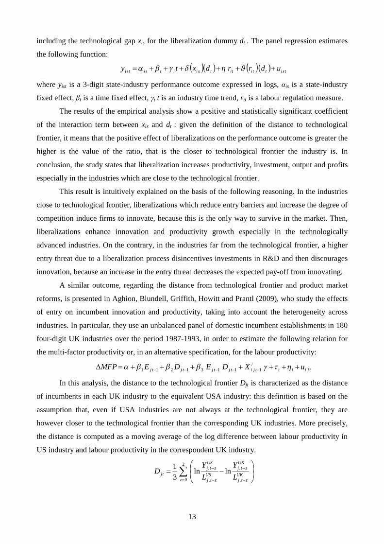
In particular, Aghion, Burgess, Redding and Zilibotti (2008) analyze the effects of the 1991

Indian Liberalization and show how the same reform may affect very differently various industries

depending on the distance from the technological frontier. They define the pre-reform distance xis to

the Indian technological frontier as the ratio of state-industry labour productivity in 1990 over the

highest state-industry labour productivity in the same year. Then they employ an interaction term

13

including the technological gap xis for the liberalization dummy dt . The panel regression estimates

the following function:

tsittititsiitsitsi udrrdxty

where yist is a 3-digit state-industry performance outcome expressed in logs, αis is a state-industry

fixed effect, βt is a time fixed effect, γi t is an industry time trend, rit is a labour regulation measure.

The results of the empirical analysis show a positive and statistically significant coefficient

of the interaction term between xis and dt : given the definition of the distance to technological

frontier, it means that the positive effect of liberalizations on the performance outcome is greater the

higher is the value of the ratio, that is the closer to technological frontier the industry is. In

conclusion, the study states that liberalization increases productivity, investment, output and profits

especially in the industries which are close to the technological frontier.

This result is intuitively explained on the basis of the following reasoning. In the industries

close to technological frontier, liberalizations which reduce entry barriers and increase the degree of

competition induce firms to innovate, because this is the only way to survive in the market. Then,

liberalizations enhance innovation and productivity growth especially in the technologically

advanced industries. On the contrary, in the industries far from the technological frontier, a higher

entry threat due to a liberalization process disincentives investments in R&D and then discourages

innovation, because an increase in the entry threat decreases the expected pay-off from innovating.

A similar outcome, regarding the distance from technological frontier and product market

reforms, is presented in Aghion, Blundell, Griffith, Howitt and Prantl (2009), who study the effects

of entry on incumbent innovation and productivity, taking into account the heterogeneity across

industries. In particular, they use an unbalanced panel of domestic incumbent establishments in 180

four-digit UK industries over the period 1987-1993, in order to estimate the following relation for

the multi-factor productivity or, in an alternative specification, for the labour productivity:

tjiittjitjtjtjtj uXDEDEMFP /11131211

In this analysis, the distance to the technological frontier Djt is characterized as the distance

of incumbents in each UK industry to the equivalent USA industry: this definition is based on the

assumption that, even if USA industries are not always at the technological frontier, they are

however closer to the technological frontier than the corresponding UK industries. More precisely,

the distance is computed as a moving average of the log difference between labour productivity in

US industry and labour productivity in the correspondent UK industry.

2

0 ,

,

,

,lnln

3

1

zUK

ztj

UKztj

USztj

USztj

tjL

Y

L

YD

14

The choice of labour productivity, instead of multi-factor productivity, doesn’t affect the

final results of the study, as it is confirmed by a robustness analysis using a measure of

technological gap based on TFP. In this case, labour productivity can be employed instead of total

factor productivity, without sensibly modifying the measure of the distance, if the intensity of

capital in the US industry and in the UK industry is approximately the same. This condition is

feasible since we are observing industrialized countries which have already reached the steady-state

level of capital per worker, such that the process of capital accumulation cannot be anymore a

source of economic growth. Then it is reasonable to assume that, if the saving rates are not so

different, the amount of capital per worker is very similar in both countries and then the intensity of

capital is almost the same.

In order to solve the endogeneity problem for the explanatory variable Ejt (foreign entry),

Aghion, Blundell, Griffith, Howitt and Prantl (2006) employ the method of two-stage least squares

to determine not only foreign entry, but also the interaction term with the technological gap. Both

foreign entry and the distance to frontier are lagged by one period with respect to the dependent

variable for two reasons: firstly, because it further avoids eventual problems of endogeneity of the

explanatory variable; secondly, because the effects of entry on incumbent innovation and

productivity are not instantaneous, given that entry threat influences the incentives of incumbent

firms and consequently induces innovation. Then the coefficient for the interaction term is negative

and significant, while the coefficient for foreign entry is positive and significant. It means that in

general foreign entry has a positive impact on productivity growth, but that this positive effect is

decreasing in the measure of the distance to frontier. If the technological gap is large, the negative

interaction term may counteract the positive impact of the pure entry variable, then explaining the

discouraging effect of liberalizations on innovation for the industries far from the frontier. On the

opposite, if the UK industries are near to the US technology frontier, the interaction term is

quantitatively negligible and then it doesn’t affect the magnitude of the positive effect of foreign

entry on the performance outcome, then illustrating the escape entry effect for technologically

advanced industries.

Some new interesting results about the interaction between market rigidities and distance to

frontier are presented in the paper by Aghion, Askenazy, Bourlès, Cette and Dromel (2009). The

aim of the study is to investigate the impact of education level, product market rigidities and

employment protection legislation on growth, by analyzing how these effects change depending on

the position of the countries relative to the technological frontier. But this article introduces some

important innovations in the examined literature: it tests the hypothesis of complementarity between

product and labour market regulations, in terms of their effect on growth; but especially it presents

the distance to frontier as a dummy variable, that equals 1 if the country's structural productivity is

15

higher than x% of US structural productivity, and 0 otherwise. In fact, a country is assumed to be

close to the frontier when its structural productivity is higher than or equal to x % of the structural

productivity in the United States. A country's structural productivity is defined as its productivity

level assuming hours worked and the employment rate are the same as in the United States. The

frontier threshold x is set at 80%, which implies that 40% of the sample is close to the technological

frontier. This choice of the dummy variable prevents from using a continuous distance to frontier

index as it would imply numerous collinearity issues with hours worked, employment rate and

productivity.

The paper exploits macro panel data for 17 OECD countries during the period 1985-2003.

The estimated relation is the following:

ititititititititititititit uCURahaERaIPMREPLaPMREPLaIHIGHaHIGHaaTFP 7652423210

where ΔTFPit is the growth rate of total factor productivity, measured by the variation in its log;

HIGHit is the level of education in the workforce, measured by the percentage of population aged

15 or over having some higher education; Iit is the dummy for the distance to frontier; EPLit and

PMRit are the OECD synthetic indicators for Employment Protection Legislation and Product

Market Regulation, used to characterise rigidities in the labour and product markets, respectively;

ΔCURit is the variation in the capacity utilisation rate, ΔERit is the change in the employment rate

and Δhit is the variation in the hours worked.

Given that the OLS estimates may be biased because of measurement errors or simultaneity

issues, the instrumental variable method is implemented. The results show a key role of the distance

to frontier in determining both the significance of some coefficients and the sign of the correlations.

For example, the coefficient for higher education is usually non-significant, but it is significantly

different from zero with positive sign when only countries close to the technological frontier are

considered. As regards the rigidities in product and labour markets, the most significant results are

obtained when rigidities in both markets are crossed and when the effects far from the frontier

(coefficient of EPLit PMRit-2 variable) are separated from those close to the frontier (sum of

coefficients of EPLit.PMRit-2 and EPLit.PMRit-2.Iit variables). In particular for such specification,

whose results are presented in column 6 of table 1, it turns out that: a one-point increase in HIGHit

has no impact on TFP for countries far from frontier but increases TFP growth by about 0.1 point

per year in countries close to frontier; a one-point decrease in overall market rigidities (that is the

product EPLit.PMRit-2) reduces TFP growth by about 0.5 point per year for countries far from the

frontier, but increases TFP growth by 0.2 point per year for countries close to frontier. Two main

conclusions arise from these results: important gains in productivity growth may be achieved in

some industrialised countries through reforms aimed at increasing education level and decreasing

16

rigidities in labour and product markets; but especially, the countries close to technological frontier

benefit from these policies much more than the countries far from the frontier.

A different conclusion, about the technological gap and the implications for economic

policy, is presented in the empirical study by Nicoletti and Scarpetta (2003), who propose a cross-

country cross-industry analysis of the relation between product market regulation and multi-factor

productivity, with the aim to study how regulation can interact with the distance from technological

frontier in order to explain the convergence process in MFP growth across different industries. For

this purpose they estimate the following function:

ijtiijtiijtitijt HPMRGapMFPPMRGapMFPLeaderMFPMFP lnlnlnln 321

where itLeaderMFPln is the growth rate of multi-factor productivity in the country leader,

ijtGapMFPln is the distance from the technological frontier, PMRi is the degree of product

market regulation in country i, Hijt is the human capital.

The authors, using an interaction term of product market regulation with the technological

gap, observe that the coefficient of the single economy-wide regulation indicator is negative but not

statistically significant, while the coefficient of the interaction term with the technological gap is

positive and statistically significant. Given that the technological gap ijtGapMFPln is defined as

the log difference of the MFP level of industry j in country i to the MFP level of that industry in the

leader country, this implies not only that product market regulation has a negative impact on TFP

growth, but also that this negative effect is quantitatively greater the wider is the technological gap.

So the existence of a stringent regulation, due to entry barriers and state control, slows down the

process of technological catch-up and this effect is particularly serious for the countries which are

farther from the technological frontier. Finally the countries that are technological laggards are the

ones which suffer the largest productivity gains from a strict regulatory environment. This is the

reason why, in this empirical framework, the most appropriate strategy of economic policy for the

technological laggards is the introduction of regulatory reforms aimed at making the economy more

market friendly.

However, the results obtained in the paper by Nicoletti and Scarpetta (2003) show an

important limit: the economy-wide regulation indicator is measured only for 1998 and it is used for

the analysis on the assumption that this one-time measure can represent the degree of product

market regulation for the entire observed period, because the regulatory patterns would not change

the relative position of each country and then its score. But this assumption doesn’t take into

account the fact that regulatory reforms and economic liberalizations were implemented by

different paces in the last years, even in the member states of the European Union involved in the

17

Single Market Program. Moreover the absence of an adequate time series for the regulation index

precludes the individuation of dynamic effects of the regulatory reforms on TFP growth: this is

reason why the coefficient for the single economy-wide index is not statistically significant. But, at

the same time, when a time-varying economy-wide indicator is constructed combining the 1998

regulation measure with the time-series indicator of liberalizations for non-manufacturing

industries, the coefficient for this explanatory variable is statistically significant at the 1% level

while the interaction term is not significant anymore. This shows that, if a time-varying indicator of

product market regulation is used, the interaction term may be not so relevant for explaining the

discussed relation.

In general, as it results from the previous considerations, the usage of the interaction term

for the explanatory variable and the technological gap is a solution frequently adopted in the recent

empirical literature regarding the effect of product market competition and foreign entry on

economic growth, in order to verify whether and how the impact may change depending on the

distance from the technological frontier. But the results of these analyses are contradictory and lead

to opposite policy implications: for Aghion, Burgess, Redding and Zilibotti (2008), for Aghion,

Blundell, Griffith, Howitt and Prantl (2009) and for Aghion, Askenazy, Bourlès, Cette and Dromel

(2009) the industries close to technological frontier need liberalizations more than the other ones for

favouring innovation, while for Nicoletti and Scarpetta (2003) the industries far from the

technological frontier require liberalizations more than the other ones for promoting innovation.

The first idea is consistent with the theory provided by Acemoglu, Aghion and Zilibotti (2006),

while the second one reflects a catch-up effect coherent with the traditional theories of convergence.

Of course, since the distance from the technological frontier may play an important role in

determining the responses of the economy to liberalization processes, it is worth to develop the

empirical analysis on this point, in order to verify what is the real interaction between economic

liberalizations and technological gap and whether the effect of this interaction may be different

depending on the way of constructing the technological gap.

1.5 Conclusions

After discussing the most important issues in the empirical literature on product market

competition and economic growth, we can draw some conclusions in order to evaluate these

solutions and also to provide some guidelines about the empirical work presented in the following

sections.

Regarding the identification of the dependent variable, we can observe that the growth rate

of total factor productivity is the best candidate among the various proposed variables. As a

18

consequence of that, the indicators of patent counts can be used just as control variables, in order to

explain the specific impact of innovation on economic growth.

Concerning the explanatory variables, we can conclude that both the index of economic

freedom and the indicator of product market regulation can be used, of course in different

specifications, as explanatory variables in the regression function. For this purpose we will structure

the empirical analysis in two sections, depending on the specific explanatory variable employed in

each part of the analysis.

Finally, the interaction between product market competition and the distance to frontier is

useful to explain how the effect of competition on productivity and growth may change depending

on the technological level of a country. This interaction term introduces some non-linearities in the

estimation of the empirical model: in fact, competition may produce a positive effect on growth for

some values of productivity levels and a negative impact for some other values of total factor

productivity. This distinction, based on the productivity level, can be applied both for different

countries, and for different industries: in our analysis, we will distinguish the various countries

included in the dataset according to the productivity level and then, thanks to this classification, we

will discuss the implementation of different solutions in terms of economic policy depending on the

distance to frontier.

19

Section A

The Impact of Economic Freedom and Distance to Frontier

on Multi-Factor Productivity

2.1 Introduction

This section aims at analyzing the relationship between product market competition and

economic growth, in particular by studying the effects of business and trade liberalizations on

technological progress, and considering the role of the distance from technological frontier in the

growth process.

The empirical approach followed in this study is determined by the policy-oriented scope of

the work. In fact, we propose a macro-level analysis based on the observation of aggregate

economies, given that it is more appropriate in order to show over time the effects of national

competition policies, which are usually conducted in a uniform way, without distinction among

industries. From this point of view, the general framework of the analysis, focused on the effect of

competition on aggregate growth, is different from the orientation of other studies, interested in the

impact of sector regulation on productivity growth of single industries. On the other hand,

regulation and competition policies work in a different way in order to promote a market-friendly

economic environment: while regulation policy operates ex ante for some specific industries, which

require a particular intervention because of their features (e.g. network industries), competition

policy functions ex post indifferently for each industry, through antitrust provisions, in order to

remedy the distortions to product market competition due to the unilateral or collusive behaviour of

firms.

The empirical analysis examines the effects of economic freedom and of the distance to

frontier on the level and on the growth rate of multi-factor productivity for a panel of 20 OECD

countries over a period 1995-2005. In particular, the study distinguishes between the indicators of

business freedom and trade freedom, as proxies for the competitive pressures coming from domestic

market and from foreign market. In fact, economic liberalizations aimed at increasing the entry of

firms in the domestic market rather than the access of foreign products may have different effects

depending on the distance from the technological frontier.

In general, considering the overall effect of the interaction term and of the economic

freedom variable, a competitive economic environment has a positive impact on economic growth,

but different policy recommendations can be formulated for trade freedom and business freedom

depending on the distance to the frontier. In fact, according to the results of the analysis, from the

perspective of economic growth, trade liberalizations are more beneficial for the countries far from

20

the frontier, because they can exploit the opportunities given by international trade also in order to

adopt the existing technologies developed by the advanced economies. On the other hand, business

liberalizations are more advantageous for the countries close to the frontier, because the elimination

of regulatory barriers increases the possibility of entry in the market and then rises the potential

competition to the incumbent firms: in this framework, both the incumbents and the entrants have

more incentives to invest in innovation, either to keep their position in the market or to successfully

enter the market. This intuition of the empirical results is also supported by the experience in many

developing countries, especially the ones which are running a transition phase from a centrally

planned economy to a market economy: in fact, we can observe that in many cases trade

liberalization has anticipated business liberalization, probably in order to attract foreign direct

investments and then to promote technological progress through the adoption of the foreign

technologies.

2.2 The data

The selection of the employed data for this analysis can be explained on the basis of the

specific motivations of the paper. Indeed, the policy implications of the analysis recommend some

criteria about the individuation of the countries to be included in the study: for this purpose, it is

necessary to consider a panel of homogenous economies, with similar characteristics, where some

of them are EU members, while other ones are not EU member states. In particular, the

homogeneity criterion is required for the countries of the sample, because it gives the possibility to

compare competition policies across countries with the same initial level of economic development

and then to observe the effects of these policies on the economy.

In fact, as suggested by the theory of relative convergence in development studies, the initial

economic conditions of the considered countries are determinant for explaining the different growth

processes and then also the different growth rates of the economies. In general, the developing

countries exploit some basic sources of economic growth such as capital accumulation or

population increase, while the industrialized states found their economic growth on the

improvement of human capital and on the advancement of technological progress. As a

consequence, in the developing economies, a competition policy aimed at increasing the number of

producers and at reducing the average size of the existing firms may delay the process of capital

accumulation, while in the industrialized nations a competition policy expected to open the market

to new competitors may encourage innovation among the incumbent firms. In conclusion, since the

growth processes follow different transmission mechanisms, depending on the level of initial

development, competition policy may be relevant or not for economic growth and may have

21

different consequences. Then, focusing the attention only on a homogenous sample, composed of

industrialized countries, should allow to derive some definite conclusions about the link

competition-innovation-growth, which is the specific object of this analysis. For this reason, the

present study considers a panel of 20 OECD countries, corresponding to industrialized economies:

Australia, Austria, Belgium, Canada, Denmark, Finland, France, Germany, Greece, Ireland, Italy,

Japan, Netherlands, New Zealand, Portugal, Spain, Sweden, Switzerland, United Kingdom, United

States.

The dependent variable used in the empirical analysis, in order to observe the impact of

competition on technological progress and so on economic growth, is the Total Factor Productivity

(TFP), called also as Multi Factor Productivity (MFP), computed for the aggregate economy. In

general, TFP is the best measure of productivity able to reflect disembodied technical change, that

is the technological progress due to a shift in the production frontier, which is not imputable to any

production input. On the opposite, embodied technical change indicates the improvement in the

design or quality of capital or intermediate goods3. In particular, we are interested in observing the

effects of economic freedom both on the level and on the growth rate of multi-factor productivity4,

in order to explain the impact of competition policy both in a static and in a dynamic perspective.

Then we employ two dependent variables: the log of total-factor productivity; the growth rate of

TFP, computed as the difference between the log of TFPt and the log of TFPt-1 as in many empirical

analyses. For this purpose, the data on Total Factor Productivity are computed5 on the basis of the

3From this point of view, we can observe a mismatch between the theoretical and the empirical literature on

competition and growth: while the first one characterizes technological innovation either as a creation of a new variety

of intermediate product (horizontal innovation) or as an improvement of the quality of existing intermediate goods

(vertical innovation), that is as different forms of embodied technical change, the second one uses as a key dependent

variable the Total Factor Productivity which, if well measured, represents an indicator of disembodied technical change.

4 More precisely, the Total-factor Productivity (TFP) is called Multi-factor Productivity (MFP) in the glossary

used in the OECD Manual on the measurement of aggregate and industry-level productivity growth. The MFP acronym

is employed in order to indicate a certain modesty with respect to the capacity of capturing the contribution to output

growth of all the factors, which don’t depend on the quantity and quality of primary and intermediate inputs.

5These data on TFP have been developed, for the database of the Research Centre in Economics and Statistics

(CREST) of the French Statistical Institute (INSEE), by Jacques Mairesse and Jimmy Lopez, that I particularly thank

for providing me with this dataset. In particular, for a given industry, the multi-factor productivity is computed as the

ratio of the domestic product over the weighted sum of the quantity of labour and the fixed stock of capital (where the

weights are given by the annual labour cost share and the capital cost share). Using these cost shares, rather than the

elasticities of output with respect to labour and capital, they depart from the assumption of perfectly competitive

markets: this is particularly useful for the peculiar scope of the analysis, which is focused on the study of markets with a

low degree of competition.

22

data for Gross Domestic Product, Capital Stock and Labour Input, provided in the OECD Statistical

Database, and are available for the cited 20 OECD countries over a period 1970-2006.

As far as it regards the explanatory variable, product market competition is defined as an

economy-wide variable, able to include two different aspects: competition in the market and for the

market. Competition in the market refers to the interaction among the firms currently operating in

the market: it may be limited by collusive agreements among oligopolist firms or by the dominant

position of monopolistic firms. Competition for the market measures the possibility for other firms

to enter and exit a market already characterized by the presence of some incumbent firms: it may be

restricted by barriers to entry or to exit, when they require a particularly high cost in terms of time

or money in order to open or close a business. The indicator of product market competition used in

this work has been individuated in the perspective of including both these elements.

Given the impossibility to use the Lerner Index because of the discussed endogeneity

problem, the variable used as a proxy for product market competition is the index of economic

freedom, computed yearly by the Heritage Foundation over a period 1995-2008. This index is an

average of 10 individual freedoms, such as business freedom, trade freedom, investment freedom,

financial freedom, property rights enforcement, freedom from corruption. In particular, business

freedom is defined as a quantitative measure of the ability to start, operate and close a business6: for

this reason the various components used for constructing this specific indicator have been identified

in order to reflect both competition in the market and competition for the market. A score between 0

and 100 is given to each component and the final result, computed as the average of equally

weighted elements, is also expressed in a scale from 0 to 100. In the empirical analysis, we will

employ both the general index and the specific indicators of economic freedom, in particular

business freedom and trade freedom.

Moreover, in order to avoid eventual endogeneity issues for the index of economic freedom,

and also in order to consider some gradualism in the impact of economic freedom on growth

process, we will use this variable not only as a real time variable but also as a lagged one. Anyway,

for the modalities of construction, the index of economic freedom can be already considered as a

lagged variable: in fact, as clarified in the presentation of the report, the index is computed on the

basis of information collected in the previous year, until the end of June, such that for example the

economic freedom indicator for 2008 reflects a situation registered between the second half of 2006

and the first half of 2007. This observation explains why the treatment of lagged variables is not so

6The objective data used for defining this indicator are the number of days and of procedures, as well as the

cost required for starting and closing a business or for obtaining a license.

23

necessary for the empirical analysis: indeed, the coefficients for the lagged variable are often not

significant, moreover their statistical significance decreases the greater is the number of time lags.

Following the recent empirical literature on competition and growth, this work takes into

account the distance from the technological frontier as a possible determinant of economic growth,

both as a single explanatory variable, and as a factor of an interaction term with the index of

economic freedom. In the first case, we are interested in examining whether the distance may have

an impact on the speed of convergence; in the second case, we want to observe whether the distance

may have an effect on the way economic freedom influences economic growth.

For the purposes of this analysis, the distance is measured as the ratio between the level of

multi factor productivity in the country j and in the technological leader country. In fact, the

productivity ratio presents some advantages with respect to other possible definitions, such as the

difference between productivity levels, because it provides a relative measure of the distance to

frontier. Given that this empirical work studies the effects of economic freedom and of distance to

frontier on MFP growth for a panel of 20 OECD countries, a relative measure of technological gap

allows a more direct comparison between the productivity levels of more than two countries. As

already said, the data on multi-factor productivity levels at constant prices are available for the

observed countries over a period 1970-2006: for all the considered years the highest level of multi-

factor productivity is registered in the USA. So the reference level of MFP, to be considered for the

computation of the distance from technological frontier, is the multi-factor productivity in the USA.

The empirical analysis also includes some control variables, which are reported in the

specification of the regression function in order to take into account other possible determinants of

economic growth. In particular, we want to measure and to distinguish the contribution given by

innovation and by imitation to economic growth: indeed, this long-run process can be promoted

both by the invention of new products and new technologies, and by the adoption of the existing

technologies developed by the leaders. So we need some control variables able to capture the

different impact of innovation and imitation on growth.

In general, an indicator of patenting activity can be considered as a good measure of

innovative output, in order to be used as a control variable in the analysis. In fact, when a new idea

is developed in the research activity, the inventors are interested in obtaining the grant of a patent in

order to exploit exclusively the output of their innovation effort: this implies that a high demand for

intellectual property protection, as well as a high amount of intellectual property rights, reflect good

results of the innovation activity.

For this reason, patent counts can be properly used as measures of innovation. In particular,

we can consider two types of indicators: the count of patents granted by the US Patent and

24

Trademark Office by priority year and the count of patent applications to the European Patent

Office by priority year, both provided by the OECD Statistical Database. These data are available

for almost the same period of time: the counts of patent applications to the EPO, classified by the

inventor’s country of residence, are computed over a period 1977-2005, while the counts of patents

granted by the USPTO, registered by the inventor’s country of residence, are reported over a period

1977-2006.

As an indicator of innovative activity, the count of patent applications to the EPO may be

more adequate than the count of patents granted by USPTO, because the application is an indicator

of innovative activity even better than the grant, which depends on an administrative procedure.

Moreover, a patent is granted some years after the application, so an indicator based on granted

patents may represent the final result of an innovative activity completed some years before7. For

these reasons, in our analysis we use the count of EPO Patent Applications as a measure of

innovative output but we also employ the count of USPTO Granted Patents for a robustness check:

in any case, the estimation of this latter specification show the same results for the effect of

innovative output on economic growth, so the choice of one of these variables doesn’t affect the

quality of the estimates.8

An alternative measure of innovative activity is the Business R&D Capital, that is the

amount of capital used by the private sector for research activity. This stock variable can be

determined as the outcome of a capitalization process, based on the flows of investments in R&D

conducted by private firms. Contrarily to the measures of patent counts, which denote the

innovation output, this variable indicates the input of innovative activity: this distinction is

fundamental in R&D activity, given that the innovation process is a stochastic one, where the

employment of some inputs (e.g. hours worked by researchers, laboratories devoted to research

activity) doesn’t imply necessarily a predefined output, because the frequency of innovation

depends on the realization of a random hazard rate. In any case, despite this stochastic element in

the innovation process, R&D capital is expected to have a positive impact on MFP, and in fact the

increase of R&D investments is indicated in policy discussions as a key strategy for promoting

technological progress and economic growth.

For the purpose of the analysis, the values of Business R&D Capital are computed by using

the method of perpetual inventory, on the basis of the OECD data on Business Enterprise

7 Nevertheless, this delay in the registration of a patent is not a particular problem for the reliability of the

counts based on USPTO granted patents because, in any case, also USPTO Granted Patents are recorded by priority

year, that is according to the year of the application.

8 For this reason, in the presentation of the analysis, we omit the results of the estimates for USPTO Granted

Patents.

25

Expenditure for R&D. These data on investment flows are measured in PPP (purchasing power

parity) millions of dollars and are available over a period 1981-20079.

By construction, this variable considers only the R&D Capital used by business sector and

then excludes the capital invested by public sector for research and development. So, in principle, it

cannot be considered as a general indicator of the amount of resources invested in a given economy

for research: in fact, the R&D capital employed by the business sector is only a fraction of the total

amount of capital devoted to research. Moreover, this fraction can be different depending on the

countries, because the composition of research expenditure varies across countries: in many states

the private component is dominant, but in some other countries the public expenditure is prevalent.

However, this observation doesn’t affect the rationale for such indicator of business R&D capital,

whose usage is justified by two reasons, a theoretical one and an econometric one.

Firstly, we want to know the specific impact of the innovation activity run by the private

sector on economic growth: in fact, only the private expenditure for research requires some

monetary incentives, such as the expectation of the monopolistic rents for the innovator, while the

public expenditure for research is determined by other - mainly political - factors. As an implication

of that, competition policy can affect only the private expenditure in R&D, by reducing the

incentives for investments, but it cannot have effect on the public expenditure in R&D.

Secondly, we have to exclude, for multicollinearity reasons, the possibility that both

business R&D capital and government R&D capital are used as control variables in the same

regression equation. In fact, even if the two components of research expenditure follow different

dynamics, these two variables are however strongly correlated and then the multicollinearity

between these two explanatory variables would sensibly affect the results of our estimations, as we

have also checked in the analysis. So, in conclusion, given that we need to know the coefficient for

the private expenditure in R&D, and since we cannot have in the same regression both the

explanatory variables for R&D Capital, the decision to keep only the first control variable is the

only feasible one.

Finally, another control variable, useful in the empirical analysis based on endogenous

growth theory, is the level of human capital. Indeed, economic growth depends not only on the flow

9 As for the data on total factor productivity, the data on the amount of capital have been computed by Jacques

Mairesse and Jimmy Lopez, for the database of the Research Centre in Economics and Statistics (CREST) of the French

Statistical Institute (INSEE). In particular, the data on the stock variable are constructed from the data on investment

flows according to the method of perpetual inventory: in fact, capital stock at the end of the year t, plus investment

minus depreciation in year t+1, give the value of the stock at the end of the year t+1. In this computation, J. Mairesse

and J. Lopez use various depreciation rates: 15% for R&D investments, 1/7 for Information Technology investments,

1/3 for soft investments, 1/15 for Communication Technology Investments. The data for investments come from the

EU-KLEMS database.

26

of discoveries and inventions which determines technological progress, but also on the

accumulation of knowledge which improves the quality and the efficiency of labour input: then a

country with better human capital should experience higher growth rates. For our purposes, human

capital is measured as the percentage of population over 25 years old, within each country, who

have some higher education. These data10 are available over a period 1970-2006. For the definition

of the variable, the country of graduation is not relevant, because also the people graduated in

foreign institutions are taken into account in the computation of the percentage. In fact, what we

want to measure in this case is not the quantitative output of the national education system, as we

could do by considering the number of graduates in each year for a given country, but the

accumulation of human capital, coming from the attendance of higher education courses. Indeed,

the mobility of students towards other countries increase the level of human capital in the economy

of their country of origin, once they come back and contribute to the production process of that

economy, especially by carrying out the tasks requiring high skill workers.

2.3 The empirical strategy

The present work adopts a cross-country time series approach, because it is aimed at

examining the effects of economic freedom and of the distance to technological frontier both on the

level and on the growth rate of multi-factor productivity for a panel of 20 OECD countries over a

period 1995-2005. Nevertheless, the estimation method for the panel analysis (that is fixed-effects

or random-effects model) changes depending on the choice of the explanatory variable used in each

set of regressions.

The econometric strategy followed for testing the relationship between TFP and the general

index of economic freedom is to estimate a panel data model with fixed effects, in order to capture

the impact of unobserved variables which are constant for each country. Indeed, given that the

growth process is determined by many sources, and since product market competition is one of the

relevant variables but not necessarily the most important one, it is necessary to take into account

other possible determinants both through the introduction of control variables in the model

specification and through the consideration of unobserved effects for missing variables. Moreover,

since these unobserved effects are often referred to country characteristics, which usually don’t

change in a short time interval, the most appropriate methodology is the fixed effects model, as

effectively confirmed by the results of the analysis. In particular, in order to choose the most correct

10These data on education are provided in Cohen D. and Soto M. (2007), Growth and Human Capital: Good

Data, Good Results, Journal of Economic Growth, vol. 12, issue 1, March, 51-76

27

model, we estimate the regression function with economic freedom as explanatory variable both by

a fixed effects model and by a GLS random effects model and we test the choice of the model on

the basis of the Hausman Test, which rejects the null hypothesis of no systematic differences

between the coefficients of the two models, given this specification of the regression function.

Then the basic specification of the regression function for this fixed effects model, before

adding any control variable, is the following one for the two dependent variables:

itititititiit uDISTEFDISTEFMFP *ln 321 (1)

itititititiit uDISTEFDISTEFMFP *321 (2)

where EFit is the general index of economic freedom in country i and time t, DISTit is the distance

to frontier for country i and in time t and EFit*DISTit is the interaction term between economic

freedom and the distance to frontier for country i and in time t.

Of course, the adoption of a fixed effects model for the cited regression excludes the

possibility to introduce in the model specification any qualitative dummy related to a country

characteristic, which is unchanged over the entire period of the analysis. For instance, this is the

case of the European Union membership: indeed, all the EU member states included in the sample,

even if they accessed the European Union in different times, were already EU members in the

period 1995-2005. For this reason, the dummy concerning EU membership always assumes the

same value for each member country (that is 1) and for each non-member state (that is 0). Given

that it is constant, the qualitative dummy plays the same role of the country fixed effect and then its

usage in the regression function of a fixed effects model implies a perfect multicollinearity problem.

Then it is necessary to drop out any country-specific constant variable, given that its effect is

already captured by the country fixed term.

On the opposite, a different econometric strategy has to be implemented for the cases where

a specific indicator of economic freedom, that is business freedom, is employed as the main

explanatory variable. Indeed, in this case, a random effects model may be preferred to a fixed

effects model, at least for the specification using TFP growth rate as a dependent variable.

The reason of this choice can be explained by the particular quality of the data, for the index

of business freedom. In fact, the score for this specific indicator, as well as for other components of

economic freedom, is mainly determined on the basis of a qualitative judgement, which implies the

assignment of a grade classifiable in a quite restricted range. For example, in the index produced by

Heritage Foundation, business freedom was initially graded according to a subjective assessment

with a score of 1-5 and only recently has been rescaled on a 0-100 basis. So, given the articulation

of such indicator, it is likely that a given country may register the same score for business freedom

over the studied time period.

28

This persistence of the same numerical value for the index of business freedom can create

some issues in the estimation of a fixed effects model, given that the country fixed term might

determine a partial multicollinearity with the examined variables. In particular, this problem is even

more serious in the case of a dynamic analysis, aimed at observing the determinants of TFP growth

over time, because a regressor always assuming the same value cannot have any explanatory power

for the variations over time of the dependent variable. So, in these cases, it could be better to use a

random effects model for estimating the empirical relation, also because these regressors are not

able to capture some unobserved effects, which are variable in time even for the same country.

In general, the random effects model allows to obtain estimates with a higher statistical

significance than the estimates computed through the fixed effects model, because it is more

efficient. But let also check, by the Hausman test, whether these estimates coming from a random

effects model are also consistent. In particular we can notice that, for the specifications including

the growth rate of TFP, the Hausman test doesn’t reject the null hypothesis of no systematic

differences between the coefficients of the two models, so we can use the random effects

specification; on the contrary, for the regressions using the log of TFP as a dependent variable, the

Hausman test rejects the null hypothesis of no systematic differences between the coefficients of the

two models, so it is safer to estimate a fixed effects model.

In conclusion, the general specification of the regression function for this random effects

model, before introducing any control variable, is the following one for the two dependent variable:

itititititit uDIST*BFDISTBFMFPln 321 (3)

itiititititit uDISTBFDISTBFMFP *321 (4)

where BFit is the indicator of business freedom in country i and time t, DISTit is the distance to

frontier for country i and in time t and BFit*DISTit is the interaction term between business freedom

and the distance to frontier for country i and in time t.

Finally, a different consideration must be proposed about trade freedom, given that this

indicator is computed on the basis both of quantitative data (concerning the amount of tariffs

towards foreign goods and services) and of qualitative assessment (regarding non-tariff barriers to

international trade). In particular, the presence of a dominant quantitative component explains why

the value of this index shows a considerable time variance. So, in this case, as for the specifications

including economic freedom, a fixed effects model is more adequate for estimating the effect of

trade freedom both on TFP level and on TFP growth. Also the results of the Hausman test confirm

this choice.

Then the basic specification of the regression function for this random effects model, before

adding any control variable, is the following one for the two dependent variables:

29

itititititiit uDIST*TFDISTTFMFPln 321 (5)

itititititiit uDIST*TFDISTTFMFP 321 (6)

where TFit is the measure of trade freedom in country i and time t, DISTit is the distance to frontier

for country i and in time t and TFit*DISTit is the interaction term between trade freedom and the

distance to frontier for country i and in time t.

2.4 The results of the analysis: the impact of economic freedom on MFP level

On the basis of the available data for the explanatory variable and for the control variables,

the empirical analysis is organized according to the following structure. In general, all the

specifications present as the main explanatory variables: the index of economic freedom (or, in

alternative, business freedom or trade freedom); the distance from the technological frontier,

measured as the ratio between multi-factor productivity levels; the interaction of the distance with

economic freedom (or, in alternative, business freedom or trade freedom), in order to understand the

role of technological gap in determining the effect of economic freedom on TFP. Tables 1-3

illustrate the estimates for the specifications described in equations 1, 3 and 5, where the dependent

variable is the log of multi-factor productivity: these results show the impact of economic freedom,

as well as of business freedom and trade freedom, on MFP level. Tables 4-6 report the results for

the specifications used in equations 2, 4 and 6, where the dependent variable is the log-difference of

multi-factor productivity: these outcomes explain the effect of economic freedom, as well as of

business freedom and trade freedom, on the growth rate of multi-factor productivity.

The results of table 1 present the effects of economic freedom and of the distance to frontier

on MFP level, as estimated through a fixed effects model. In particular, some interesting results,

from the viewpoint of the economic interpretation, are obtained in columns 3-4 of table 1: there we

can observe a positive and significant (at 1% level) relation between economic freedom and TFP;

the interaction term has a negative and significant (at 1% level) effect on MFP growth, even

variable depending on the specifications. Given that both the coefficient for economic freedom and

the coefficient for the interaction term are statistically significant, the total effect of economic

freedom must be determined considering the sum of the two terms having opposite signs. Anyway,

looking at the single specifications, the coefficient of economic freedom in absolute value is

approximately equal to 7/10 of the parameter for the interaction term. Then, given the construction

of the distance variable, the positive impact of the interaction term prevails on the negative effect of

the single regressor for productivity ratio values higher than 7/10. It means that the countries having

a lower productivity level experience a global positive effect from economic freedom: then

economic liberalizations increase MFP level in the countries which are farther from the frontier,

30

Table 1. The effects of economic freedom and of distance to frontier on the level of MFP

Dep. Var.: lnMFP (1) (2) (3) (4)

Distance to Frontier 1.882645***

(0.1966038)

1.803726***

(0.1969833)

Economic Freedom 0.0010998*

(0.0006634)

0.0012993*

(0.0006937)

0.0077957***

(0.0017351)

0.0071232***

(0.0017366)

Economic Freedom*Distance -0.0115434***

(0.0025167)

-0.0107962***

(0.0025039)

Higher Education 0.0018355

(0.0016537)

0.0016168

(0.0016687)

0.0043325***

(0.000895)

0.0046761***

(0.0008955)

(Ln) Capital Business R&D 0.0815969***

(0.0163347)

0.087263***

(0.0173224)

0.0119936

(0.011224)

0.0129366

(0.0110781)

(Ln) ICT Capital 0.0588223***

(0.0082217)

0.0547841***

(0.0091907)

0.0855454***

(0.00557)

0.0848996***

(0.0055011)

EPO Patent Counts 0.0000013

(0.0000013)

0.0000025***

(0.000007)

-0.0000015

(0.0000019)

EPO Patent Counts*Distance 0.0000054**

(0.0000024)

Constant 1.584711***

(0.1009886)

1.557293***

(0.1047755)

0.7139662***

(0.1271635)

0.7696467***

(0.1277824)

Country fixed dummy YES YES YES YES

Notes: - The symbols ***, **, * indicate respectively a significance level of 1%, 5% and 10%.

- The estimation with a country fixed effect corresponds to a fixed-effects panel data model.

with respect to this threshold. Regarding the control variables, we can notice that ICT capital

always has a positive and significant effect on MFP level. Also business R&D capital and EPO

patent counts show positive coefficients, but they are alternatively significant. In fact, the two

variables are strongly correlated, because they can be considered respectively as indicators of the

input and of the output of innovative activity: for this reason, when the coefficient for business

R&D capital is significant, the coefficient for patent counts is not, and vice versa.

Then, in the following two tables, specific components of economic freedom are used,

instead of the general index of economic freedom, as explanatory variables in the regression

function. In particular, business freedom is proposed as an indicator of the competitive pressures

due to the internal market, because of the existence of other producers or the entry of new firms. On

the opposite, trade freedom is suggested as a measure of the possible competition coming from

external market, through the supply of foreign products imported without trade barriers.

Table 2 shows the estimates of a fixed-effect model, where the main explanatory variables

of the regression function are the index of business freedom and its interaction with the distance

31

Table 2. The effects of business freedom and of distance to frontier on the level of MFP

Dep. Var.: lnMFP (1) (2) (3) (4)

Distance to Frontier 1.550865***

(0.1472912)

1.483354***

(0.1502953)

Business Freedom 0.0006316*

(0.0003506)

0.0006511*

(0.0003526)

0.0044694***

(0.0010671)

0.0040657***

(0.0010791)

Business Freedom*Distance -0.0067061***

(0.0016999)

-0.006133***

(0.0017121)

Higher Education 0.002227

(0.0016781)

0.0020926

(0.0016952)

0.0041434***

(0.0009241)

0.0044376***

(0.0009292)

(Ln) Capital Business R&D 0.0712598***

(0.0184563)

0.0749119***

(0.0194103)

0.0220374*

(0.0116687)

0.0226163*

(0.0115727)

(Ln) ICT Capital 0.0650532***

(0.0086791)

0.0628874***

(0.0093737)

0.0789504***

(0.0053485)

0.0781671***

(0.0053187)

EPO Patent Counts 0.0000008

(0.0000013)

0.0000026***

(0.0000007)

-0.0000007

(0.0000019)

EPO Patent Counts*Distance 0.0000045*

(0.0000024)

Constant 1.6375***

(0.1051418)

1.622498***

(0.1080932)

0.9203433*

(0.1065909)

0.9638104***

(0.1081285)

Country fixed dummy YES YES YES YES

Notes: - The symbols ***, **, * indicate respectively a significance level of 1%, 5% and 10%.

- The estimation with a country fixed effect corresponds to a fixed-effects panel data model.

Business freedom produces a positive and significant effect on MFP level, while the interaction

term presents a negative and significant coefficient: the overall effect of business freedom on MFP

level is positive for the countries far from the frontier (i.e., given the value of the coefficients, with

a productivity level lower than 2/3 of the TFP level in the leader country), while it is negative for

the economies close to the frontier. For the control variables, the same observations proposed for

table 1 hold also for the results of table 2.

Table 3 illustrates the effects of trade freedom and of the distance to frontier on MFP level,

using the estimates of a fixed-effects model. Trade freedom, as a single variable, always has a

positive and significant impact on MFP level, even if the coefficient presents quite different values

depending on the specifications. The interaction between trade freedom and the distance to frontier

shows a negative and significant (in col.4-6) coefficient. So, comparing the coefficients of the two

explanatory variables, we can conclude that the positive impact of trade freedom counteracts the

negative effect of the interaction term for the countries far from the technological frontier, and vice

versa for the economies close to the frontier. For example, let consider the specification in col.5: in

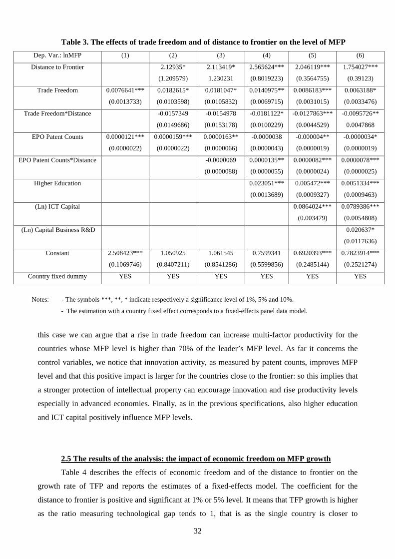
32

Table 3. The effects of trade freedom and of distance to frontier on the level of MFP

Dep. Var.: lnMFP (1) (2) (3) (4) (5) (6)

Distance to Frontier 2.12935*

(1.209579)

2.113419*

1.230231

2.565624***

(0.8019223)

2.046119***

(0.3564755)

1.754027***

(0.39123)

Trade Freedom 0.0076641***

(0.0013733)

0.0182615*

(0.0103598)

0.0181047*

(0.0105832)

0.0140975**

(0.0069715)

0.0086183***

(0.0031015)

0.0063188*

(0.0033476)

Trade Freedom*Distance -0.0157349

(0.0149686)

-0.0154978

(0.0153178)

-0.0181122*

(0.0100229)

-0.0127863***

(0.0044529)

-0.0095726**

0.0047868

EPO Patent Counts 0.0000121***

(0.0000022)

0.0000159***

(0.0000022)

0.0000163**

(0.0000066)

-0.0000038

(0.0000043)

-0.000004**

(0.0000019)

-0.0000034*

(0.0000019)

EPO Patent Counts*Distance -0.0000069

(0.0000088)

0.0000135**

(0.0000055)

0.0000082***

(0.0000024)

0.0000078***

(0.0000025)

Higher Education 0.023051***

(0.0013689)

0.005472***

(0.0009327)

0.0051334***

(0.0009463)

(Ln) ICT Capital 0.0864024***

(0.003479)

0.0789386***

(0.0054808)

(Ln) Capital Business R&D 0.020637*

(0.0117636)

Constant 2.508423***

(0.1069746)

1.050925

(0.8407211)

1.061545

(0.8541286)

0.7599341

(0.5599856)

0.6920393***

(0.2485144)

0.7823914***

(0.2521274)

Country fixed dummy YES YES YES YES YES YES

Notes: - The symbols ***, **, * indicate respectively a significance level of 1%, 5% and 10%.

- The estimation with a country fixed effect corresponds to a fixed-effects panel data model.

this case we can argue that a rise in trade freedom can increase multi-factor productivity for the

countries whose MFP level is higher than 70% of the leader’s MFP level. As far it concerns the

control variables, we notice that innovation activity, as measured by patent counts, improves MFP

level and that this positive impact is larger for the countries close to the frontier: so this implies that

a stronger protection of intellectual property can encourage innovation and rise productivity levels

especially in advanced economies. Finally, as in the previous specifications, also higher education

and ICT capital positively influence MFP levels.

2.5 The results of the analysis: the impact of economic freedom on MFP growth

Table 4 describes the effects of economic freedom and of the distance to frontier on the

growth rate of TFP and reports the estimates of a fixed-effects model. The coefficient for the

distance to frontier is positive and significant at 1% or 5% level. It means that TFP growth is higher

as the ratio measuring technological gap tends to 1, that is as the single country is closer to

33

technological frontier: but this positive effect of the distance to frontier on MFP growth might be

affected by a potential endogeneity problem, so this result could require a robustness check on the

basis of further analysis. In the specifications including only economic freedom as the main

explanatory variable, this regressor shows a negative and significant coefficient. On the opposite, in

the specifications containing both the single explanatory variable and the interaction term, we

observe that economic freedom, at least in col.5 and 6, has a positive and significant (at 10% level)

effect on MFP growth, while the interaction term with the technological gap shows a negative and

significant result at 5% or 10% level. It implies that, if the single explanatory variable is not

significant, economic freedom has a negative impact and this effect on TFP growth is quantitatively

greater for the countries which are closer to the technological frontier (whose productivity levels

ratio is higher). Instead, if the single explanatory variable is significant, economic liberalizations

may positively affect growth performance, but only for laggard economies, provided that their

multi-factor productivity level is lower than 50% of the leader’s MFP. Notwithstanding the broad

Table 4. The effects of economic freedom and of the distance to frontier on MFP growth

Dep. Var.: ΔlnMFP (1) (2) (3) (4) (5) (6)

Distance to Frontier 0.1081007**

(0.0432004)

0.4008789**

(0.1678393)

0.5246798***

(0.185933)

0.579626***

(0.1872118)

0.6676913***

(0.2127998)

0.6902668***

(0.2131454)

Economic Freedom -0.0010611***

(0.0003015)

0.0018348

(0.0016326)

0.0020538

(0.0016995)

0.0025973

(0.0017152)

0.0032424*

(0.0018689)

0.0035485*

(0.0018811)

Economic Freedom*Distance -0.004222*

(0.0023398)

-0.0050541**

(0.0024807)

-0.0054865**

(0.0024754)

-0.0064802**

(0.0027264)

-0.0067314**

(0.0027285)

Higher Education 0.0003276

(0.0005872)

0.0014842*

(0.0008741)

0.0011296

(0.0009645)

0.0009771

(0.0009703)

(Ln) Business R&D Capital -0.0139696*

(0.0078657)

-0.0216581*

(0.0118137)

-0.0178735

(0.0121683)

(Ln) ICT Capital 0.0049141

(0.0056302)

0.0021316

(0.0060386)

EPO Patent Counts 0.000001

(0.000001)

Constant 0.0149342

(0.0361615)

-0.1858446

(0.1169284)

-0.2521367*

(0.1280227)

-0.1919378

(0.1315718)

-0.2201145

(0.1355746)

-0.25333*

(0.1378626)

Country fixed dummy YES YES YES YES YES YES

Notes: - The symbols ***, **, * indicate respectively a significance level of 1%, 5% and 10%.

- The estimation with a country fixed effect corresponds to a fixed-effects panel data model.

34

coverage of the index of economic freedom, we can argue that this result about the negative impact

of competition on growth, especially for the leader economies, is consistent anyway with the

Schumpeterian idea of monopoly as necessary reward for innovation.

Tables 5 and 6 present the results of the estimation of a regression function, where the

explanatory variables are respectively business freedom and trade freedom. In particular, table 5

presents the estimates of a random-effects model, for the reasons explained in the previous

paragraph. Given the results for the main explanatory variables (negative coefficient for business

freedom and positive coefficient for the interaction with the distance to frontier), we can observe

that business liberalizations are more beneficial for MFP growth in the countries closer to

technological frontier rather than for the growth performance in the economies far from the frontier.

Finally, the coefficient for the distance to frontier is always significant and negative, which implies

that MFP growth rate is higher the lower is the productivity ratio: then the countries far from the

frontier register a higher growth rate than the technologically leader economies, as supported by the

Table 5. The effects of business freedom and of the distance to frontier on MFP growth

Dep. Var.: ΔlnMFP (1) (2) (3) (4) (5)

Distance to Frontier -0.1938833

(0.118146)

-0.1937736*

(0.1142223)

-0.1932168*

(0.1018266)

-0.1582389

(0.1069505)

-0.1570887

(0.1063468)

Business Freedom -0.0015496*

(0.0009358)

-0.0016406*

(0.0009082)

-0.0016523**

(0.000819)

-0.0014701*

(0.0008778)

-0.0014274

(0.0008756)

Business Freedom*Distance 0.0025613*

(0.0014476)

0.0026907*

(0.0014011)

0.0026088**

(0.0012523)

0.0023967*

(0.0013446)

0.0023048*

(0.0013426)

Higher Education -0.0001752

(0.0001994)

-0.0000071

(0.0002001)

0.0001113

(0.0001669)

0.0001543

(0.0001706)

0.0001455

(0.0001685)

(Ln) Business R&D Capital -0.0022075**

(0.00097)

0.003069*

(0.0016868)

0.0016825

(0.0018418)

(Ln) ICT Capital -0.006512***

(0.0019042)

-0.0062256***

.0014086

-0.0075706***

(0.0020462)

EPO Patent Counts 0.0000017**

(0.0000008)

0.0000014*

(0.0000008)

EPO Patent Counts*Distance -0.0000001

(0.0000009)

-0.000001

(0.0000009)

Constant 0.1356614*

(0.0764151)

0.1542183**

(0.0744323)

0.1766702***

(0.0670834)

0.173031**

(0.0686694)

0.1726132**

(0.0683172)

Country fixed dummy NO NO NO NO NO

Notes: - The symbols ***, **, * indicate respectively a significance level of 1%, 5% and 10%.

- The estimation with a country fixed effect corresponds to a fixed-effects panel data model. The estimation

without the country fixed effect is GLS estimation of a random-effects panel data model.

35

theory of convergence 11. Moreover we also observe, for the control variables, that the adoption of

ICT technologies can have a negative impact on MFP growth while intellectual property protection

generally produces a positive effect. These results obtained for business freedom are also confirmed

and even strengthened by a robustness check, as we can notice from table A.1 in the Appendix. In

particular, in that table, we present the estimates for the same regression, where the distance to

frontier is used as a one-year or two-year lagged variable. In this way, we can rule out the

hypothesis that such results for the specification including business freedom can be influenced by

an eventual endogeneity of the distance to frontier: in fact, we have to remember that the dependent

variable is the log difference of MFP levels in time t and in time t-1 for a given country, while the

distance to frontier is defined as the ratio of MFP levels in country j and in the leader country.

Table 6. The effects of trade freedom and of the distance to frontier on MFP growth

Dep. Var.: ΔlnMFP (1) (2) (3) (4)

Distance to Frontier 0.8809255**

(0.3864873)

0.9254229**

(0.4153367)

1.009026**

(0.4136151)

0.9942031**

(0.4232292)

Trade Freedom 0.0063304*

(0.0033459)

0.0066677*

(0.0035412)

0.0073309**

(0.003524)

0.0071913**

(0.0036214)

Trade Freedom*Distance -0.0089891*

(0.0047642)

-0.0094776*

(0.0050511)

-0.0103631**

(0.0050238)

-0.0101515*

(0.0051783)

Higher Education 0.0015804*

(0.0009173)

0.0014619

(0.0010021)

0.0012105

(0.0010008)

0.0011751

(0.0010236)

(Ln) Business R&D Capital -0.0249526***

(0.0079757)

-0.0277234**

(0.0122555)

-0.0209877*

(0.0126127)

-0.0207469

(0.0127258)

(Ln) ICT Capital 0.0016632

(0.0055732)

-0.0024776

(0.0059075)

-0.0025077

(0.0059291)

EPO Patent Counts 0.0000015*

(0.0000008)

0.0000018

(0.0000021)

EPO Patent Counts*Distance -0.0000048

(0.0000027)

Constant -0.3852514

(0.2581847)

-0.4042711

(0.2666889)

-0.4893993*

(0.2676931)

-0.480924*

(0.2727492)

Country fixed dummy YES YES YES YES

Notes: - The symbols ***, **, * indicate respectively a significance level of 1%, 5% and 10%.

- The estimation with a country fixed effect corresponds to a fixed-effects panel data model.

11 In the following analysis, similar results will be obtained in table 6 of the second analysis, where, on the

opposite, the explanatory variable is product market regulation.

36

Table 6 presents the fixed-effects estimates for the regression function including trade

freedom as the main explanatory variable. As we have noticed also for the general index of

economic freedom, trade freedom has a positive coefficient, while its interaction with the distance

to frontier shows a negative coefficient: combining the two countervailing effects, we can conclude

that trade freedom induces a positive impact on economic growth for the countries far from the

frontier (having a productivity level lower than 70% of TFP level in the leader country), while it

reduces the growth rate of total factor productivity for the technologically advanced countries.

Finally, comparing the results in tables 5 and 6, we can draw different conclusions about the

interaction between the specific component of economic freedom (business freedom or trade

freedom) and the distance to frontier: business freedom is more beneficial for economic growth in

the countries close to the frontier, while trade freedom can increase TFP growth rates especially for

the economies far from the frontier. But in general, we can argue that the results obtained for

business freedom are more robust than the ones computed for trade freedom: in fact, the

introduction of time lags for the definition of the distance to frontier doesn’t affect the estimates for

the regression including business freedom; on the opposite, the outcomes for trade freedom are not

confirmed by an analogous robustness check.

2.6 Conclusions

This empirical study has analyzed the impact of economic freedom and of the distance to

frontier on the level and on the growth of multi-factor productivity. In particular, within this

framework, the indices of business freedom and trade freedom have been employed as specific

indicators for two different types of competitive pressures, that is the competition due to the entry

or the activity of other firms in the same market, and the access of foreign products sold in the

domestic market. Probably, a more complete empirical framework should also include some data

about greenfield entry, given that another type of competitive pressures could also come from the

foreign direct investments of firms interested in creating new establishments. But the index of

investment freedom, provided by the Heritage Foundation and included in the computation of the

general index, is based fundamentally on qualitative judgements and not on quantitative data, and

then it doesn’t provide accurate information on this relevant aspect.

Given the results of this study, we must observe that, notwithstanding the specific effect of

economic freedom on TFP level or on TFP growth, no general conclusion can be drawn about the

relationship between competition and growth without considering the role of the distance to frontier

both in determining the speed of convergence process and especially in influencing the effects of

competition policies on the growth rate of total factor productivity.

37

Among the various estimates of the regression function for the growth rate of multi-factor

productivity, we consider with particular attention the specification including business freedom as

the main explanatory variable, given the good results obtained from the robustness check. In fact, in

such case, also the usage of time lags has confirmed the positive effect of technological gap on TFP

growth: the countries far from the technological frontier grow faster than the economies at the

frontier, because the first ones may also imitate the advanced technologies of foreign countries

while the second ones need to innovate in order to promote productivity growth. Moreover,

regarding the interaction term, we can notice that the interaction has the effect to reinforce the

positive impact, or at least to reduce the negative impact of business liberalizations in the countries

closer to the technological frontier.

Finally, as we can notice from the outcomes of the analysis, the choice to employ both the

level and the growth rate of MFP as dependent variables is useful in order to evaluate the impact of

competition policies and of other policies both in the short and in the long run. In fact, given that in

some cases the effect of the same explanatory variable on MFP level and on MFP growth is

different in sign, this approach also allows to show the trade-off between static efficiency and

dynamic efficiency, which we have pointed out in the model described in chapter 2. For example,

competition policy usually has positive effects on TFP levels, because it increases static efficiency,

but in several cases it can also have a negative impact on TFP growth, since it reduces dynamic

efficiency.

38

Section B

The Impact of Product and Labour Market Rigidities

and of Distance to Frontier on Multi-Factor Productivity

3.1 Introduction

In this section we are interested in analyzing the effects of product and labour market

rigidities and of higher education on the level and on the growth rate of multi-factor productivity. In

this way such empirical analysis aims at testing some of the predictions proposed by endogenous

growth theory and at tackling some relevant issues of the current debate on the design of growth-

enhancing policies.

Firstly, we want to examine the impact of product market regulation on the rate of

technological progress, as measured by multi-factor productivity, in order to define the sign and the

magnitude of this effect. In fact, given that liberalization and deregulation policies are often

indicated in the agenda for a growth-improving strategy, we seek to understand which of the effects

predicted in the theoretical literature, that is the Schumpeterian one or the escape competition one,

effectively prevails. In particular, in this analysis, we focus our attention on product market

regulation in some non manufacturing industries, such as energy, transport and communication.

So, given that we are considering the effects of regulation in public utilities, peculiarity of

our data for the explanatory variable, the conclusions of this analysis will be partially affected by

the specific features of these network industries, with a crucial role of public sector. For this reason,

it is also important to disentangle the different effects of product market regulation and public

sector intervention, given that the two elements are jointly considered in the construction of our

index, provided by OECD database.

Secondly, we are interested in observing the impact of employment protection legislation on

multi-factor productivity, in order to understand the effect of the reforms aimed at increasing the

degree of flexibility in labour market. In particular, since current legislation provides different

forms of employment protection for regular and transitory contracts, it is also useful to distinguish

the effects depending on the form of contract, eventually in order to understand what type of labour

market reform can affect more significantly the rate of technological progress.

Moreover, also this work takes into account the distance from the technological frontier as a

factor of an interaction term with the main explanatory variables. The aim is to observe whether the

distance may have an effect on the way product market regulation, employment protection

legislation and higher education influence technological progress and economic growth.

39

3.2 The Empirical Analysis

For this study, we employ the same dataset used in the previous analysis, as far it concerns

the dependent variables (the values of multi-factor productivity), as well as the control variables

(business R&D capital, ICT capital, higher education). The main explanatory variables are different,

given that we use two indicators of product and labour market rigidities, constructed by OECD,

which are product market regulation and employment protection legislation. Also in this analysis,

the two indicators of product and labour market rigidities are interacted with the distance from the

technological frontier, which is measured as the ratio between the level of multi-factor productivity

in the country j and in the technological leader country.

The empirical strategy of this study is to estimate a panel data model with fixed effects, in

order to capture the impact of unobserved variables which are constant for each country. In

particular, in order to choose the most correct model, we estimated the regression function both by a

fixed effects model and by a GLS random effects model and we tested the choice of the model on

the basis of the Hausman Test, which always rejected the null hypothesis of no systematic

differences between the coefficients of the two models, given this specification of the regression

function. This is the reason why sometimes the results in the tables are just the ones referred to the

fixed-effects specification.

In order to analyze the different proposed issues, we will use different specifications and

then we will present the results separately for each of them. In particular, we will discuss in tables

1-5 the results obtained for the impact of product market regulation and employment protection

legislation on the level of multi-factor productivity, while in table 6 we will present the estimations

for the effect of the cited product and labour market rigidities on the growth rate of MFP.

3.2.1 The basic analysis: the role of ICT capital and of rigidities in labour contracts

The basic specification of the regression function, before adding any interaction term, is the

following one:

ititititititiit uKTIClnKBRDlnHIGHEPLETCRMFPln 54321 25

where lnMFPit is the log of multi-factor productivity in country i and time t, ETCRit is the index of

product market regulation, EPLit is the index of employment protection legislation, HIGH25it is the

percentage of population over 25 years old with some higher education, lnKBRDit is the log of

business R&D capital and lnKTICit is the log of ICT capital.

The results presented in table 1 show that product market regulation and employment

protection legislation have negative effect on multi-factor productivity, while business R&D capital

and ICT capital have a positive impact. In particular, considering the specification in column 1, we

40

Table 1. The effects of market rigidities, education and ICT capital stock on MFP

Dep. Var.: ln MFP (1) (2) (3) (4)

EPL

Regular Contracts

-0.0373**

(0.0173)

-0.0291*

(0.0170)

-0.0662***

(0.0171)

-0.0596***

(0.0168)

ETCR-0.0219***

(0.0040)

-0.0274***

(0.0042)

-0.0032

(0.0048)

-0.0065

(0.0051)

Higher Education 0.0016

(0.0012)

0.0021*

(0.0012)

-0.0010

(0.0012)

-0.00067

(0.0013)

(Ln) Business R&D Capital 0.1917***

(0.0095)

0.1676***

(0.0092)

0.1389***

(0.0123)

0.1164***

(0.0123)

(Ln) ICT Capital 0.0600**

(0.0096)

0.0632***

(0.0100)

Constant1.3172

(0.1090)

1.5469***

(0.1161)

1.2458***

(0.1042)

1.4240***

(0.1123)

Country fixed effect YES NO YES NO

Notes: - The symbols ***, **, * indicate respectively a significance level of 1%, 5% and 10%.

- The estimation with a country fixed effect corresponds to a fixed-effects panel data model. The estimation

without the country fixed effect is GLS estimation of a random-effects panel data model.

can observe that a one-point increase in ETCR implies a 0.022% decrease in MFP, while a one-

point increase in EPLR determines a 0.037% reduction. Moreover, a one-percent rise in KBRD

produces a MFP growth equal to 0.19%, showing a very important effect of R&D capital on multi-

factor productivity growth: in fact, as it will be confirmed in almost all the cases, this is the

explanatory variable with the most important effect on MFP.

Our measure of multi-factor productivity MFP is computed without including the role of

ICT. Thanks to this choice, we can include ICT capital as an explanatory variable, and then also

compare the different impact of the two main control variables, that is KBRD and KTIC, on multi-

factor productivity. And in fact the introduction of KTIC significantly changes the estimates, as

shown in column 3. ETCR is no more significant, while EPLR still produces a negative impact and

presents a coefficient almost double in magnitude than before (-0.066). Education is not significant

as before. A one-percent increase in KBRD implies a 0.14% rise in MFP, while a one-percent

growth in KTIC is associated to a 0.06% augmentation in MFP. As expected, the addition of KTIC

reduces the coefficient for KBRD, given that it previously captured the effects of the two variables:

moreover we can observe that R&D activity contributes to technological progress more than the

adoption of ICT technology, as confirmed in most of the subsequent results, where the coefficient

41

Table 2. The role of rigidities in regular and transitory labour contracts.

Dep. Var.: ln MFP (1) (2) (3) (4) (5) (6)

EPL

Regular Contracts

-0.0662***

(0.0171)

-0.0597***

(0.0168)

-0.0622***

(0.0168)

-0.0560***

(0.0167)

EPL

Transitory Contracts

-0.0161***

(0.0043)

-0.01478***

(0.0044)

-0.0150***

(0.0042)

-0.0133***

(0.0044)

ETCR-0.0032

(0.0048)

-0.0065

(0.0051)

0.0053

(0.0055)

0.0021

(0.0056)

0.00568

(0.0054)

0.0017

0.0056

Higher Education -0.0010

(0.0012)

-0.0007

(0.0013)

0.0006

(0.0012)

0.0008

(0.0012)

-0.0006

(0.00122)

-0.0003

0.0013

(Ln) Business R&D

Capital

0.1389***

(0.0123)

0.1164***

(0.0123)

0.1537***

(0.0121)

0.1350***

(0.0120)

0.1434***

(0.0122)

0.1221***

(0.0122)

(Ln) ICT Capital 0.0599***

(0.0096)

0.0632***

(0.0099)

0.0538***

(0.0093)

0.0565***

(0.0096)

0.0629***

(0.0095)

0.0657***

(0.0098)

Constant1.2458***

(0.1042)

1.4240***

(0.1123)

1.0002***

0.0993

1.1598***

(0.1096)

1.1519***

(0.1058)

1.3243***

(0.1150)

Country fixed effect YES NO YES NO YES NO

Notes: - The symbols ***, **, * indicate respectively a significance level of 1%, 5% and 10%.

- The estimation with a country fixed effect corresponds to a fixed-effects panel data model. The estimation

without the country fixed effect is GLS estimation of a random-effects panel data model.

for KBRD is at least twice as bigger as the coefficient for KTIC. At the same time, the results for

ETCR and EPLR require some explanation: we can eventually argue that, since the usage of ICT

technology may reduce the demand for labour, especially for non-skilled workers, more flexibility

in the labour contracts is required in a ICT-based economy, in order to reduce labour market

rigidities and to improve technological progress; so the larger coefficient for employment protection

legislation could reflect that.

The results presented in table 2 allow for a comparison between the two components of

employment protection legislation, that is regular contracts (EPLR) and transitory contracts (EPLT).

In table 1 we have used EPLR because we consider it as a more reliable indicator of labour market

rigidities, because of the construction of the data for EPLT. Nevertheless, we are interested in

observing the different impact of these variables on MFP: so, when we use just one variable, the

coefficient for EPLR is equal to -0.066 (col.1), while the coefficient for EPLT is equal -0.016 (col.3).

The results don’t change much if we use both variables in the same specification (col.5): then, the

coefficient for EPLR is -0.056 and for EPLT is -0.013. This means that, even if employment

42

protection legislation usually has a negative impact on MFP, this effect is much larger for regular

contracts than for transitory contracts.

3.2.2 Adding the interaction between product and labour market rigidities

In this second approach we are interested in analyzing the cross-interaction effects between

product market regulation and employment protection legislation. Indeed, we notice that rigidities

in product market and labour market are strongly correlated, since countries with high product

market regulation often present a quite rigid legislation on employment protection. Starting from

this observation, the hypothesis that we want to test is whether these rigidities may have a

complementary effect on productivity, as proposed in the analysis by Aghion, Askenazy, Bourlès,

Cette and Dromel (2009): because of such complementarity, the interaction term between the

rigidities in goods and labour market should be considered as an important determinant of multi-

factor productivity, since it would capture an overall effect not considered in the estimations for the

single indicators as explanatory variables. For this reason, we extend our analysis by including such

interaction term to the previous specification, in order to compare the impact of the interaction term

with the effects of the single indicators of market rigidities.

Then the specification of the regression function, after adding this interaction term, is the

following one:

ititititititititiit uKTIClnKBRDlnHIGHEPL*ETCREPLETCRMFPln 654321 25

where ETCRit*EPLit is the interaction term between product market regulation and employment

protection legislation in country i and time t.

In table 3 we present the results for the case where the indicator of goods market rigidities is

ETCR, that is the general indicator of product market regulation which includes the component of

the public sector. In column 1, we estimate the regression with ETCR and EPL as distinct variables:

ETCR is not significant, while EPL shows a negative coefficient equal to -0.037. In column 3, we

run the regression which only includes the interaction term ETCR*EPL: it has a negative coefficient

equal to -0.003, then it implies that the overall effect of market rigidities on MFP4 is however

negative. Finally, in column 5, we present the results for a regression function with ETCR, EPL and

ETCR*EPL as main explanatory variables: here we observe no significant coefficient for EPL, a

significant and positive coefficient for ETCR (0.016) and a significant and negative coefficient for

ETCR*EPL (-0.004). While the outcome for the interaction term has the expected sign, the positive

coefficient for ETCR is quite surprising compared to all the other results. We suppose that this

unusual result is due the peculiar construction of the index of product market regulation, also

including the subcomponent for public sector.

43

Table 3. The interaction between product and labour market rigidities.

Dep. Var.: ln MFP (1) (2) (3) (4) (5) (6)

EPL-0.0366***

(0.0080)

-0.0332***

(0.0082)

-0.0155

(0.01459)

-0.0104

(0.0154)

ETCR0.0068

(0.0054)

0.0029

(0.0056)

0.0161**

(0.0076)

0.0110

(0.0081)

ETCR*EPL-0.0034***

(0.0009)

-0.0036***

(0.0009)

-0.0039*

(0.0023)

-0.0040*

(0.0024)

Higher Education 0.0002

(0.0012)

0.0004

(0.0012)

-0.0003

(0.0012)

0.0001

(0.0012)

0.0003

(0.0012)

0.0007

(0.0012)

(Ln) Business R&D

Capital

0.1525***

(0.0119)

0.1308***

(0.0119)

0.1525***

(0.0119)

0.1330***

(0.0117)

0.1501***

(0.0120)

0.1196***

(0.0120)

(Ln) ICT Capital 0.05656***

(0.0093)

0.0597***

(0.0096)

0.0452***

(0.0076)

0.0509***

(0.0077)

0.0602***

(0.0095)

0.0647***

(0.0101)

Constant1.0262

(0.0964)

1.2080***

(0.1058)

1.1330***

(0.0740)

1.2590***

(0.0864)

0.9638***

(0.1027)

1.2183***

(0.1103)

Country fixed effect YES NO YES NO YES NO

Notes: - The symbols ***, **, * indicate respectively a significance level of 1%, 5% and 10%.

- The estimation with a country fixed effect corresponds to a fixed-effects panel data model. The estimation

without the country fixed effect is GLS estimation of a random-effects panel data model.

For this reason, in table 4 we show the results for a slightly different specification, where the

impact of public sector is separately considered, that is:

itititititit

ititititiit

uURHPWlnKTIClnKBRDlnHIGH

EPL*ETCRNOPUBEPLPUBETCRNOPUBMFPln

98765

4321

25

where ETCRNOPUBit is the index of product market regulation without public sector for country i

and in time t, PUBit is the indicator of public sector presence in the considered industries,

ETCRNOPUBit*EPLit is the interaction between product market regulation (without public sector)

and employment protection legislation, lnHPWit is the log of numbers of hours per worker and UR

is the unemployment rate. In particular, the latter two explanatory variables are added in order to

control for the cyclical effects which can influence the level of multi-factor productivity.

As before, in column 1, we estimate the regression with ETCRNOPUB, PUB and EPL as

distinct variables: but this time ETCRNOPUB has a negative and significant (even at 10% level)

coefficient equal to -0.010, while EPL shows a negative and significant coefficient equal to -0.033

and, what’s more important, PUB presents a positive and significant coefficient equal to 0.013. This

means that, when public sector is autonomously considered, the rigidities on the market of goods

44

Table 4. The interaction between product (without public) and labour market rigidities

Dep. Var.: ln MFP (1) (2) (3) (4) (5) (6)

EPL -0.0331***

(0.0079)

-0.0293***

(0.0080)

-0.0068

(0.0150)

-0.0091

(0.0155)

ETCRNOPUB -0.00980*

(0.0050)

-0.0159***

(0.0051)

0.0018

(0.0076)

-0.0095

(0.0078)

ETCRNOPUB*EPL -0.0053***

(0.0008)

-0.0056***

(0.0009)

-0.0049**

(0.0023)

-0.0035

(0.0024)

PUB 0.0134***

(0.0051)

0.0183***

(0.0052)

0.0139***

(0.0047)

0.0164***

(0.0048)

0.0128**

(0.0051)

0.0195***

(0.0053)

Higher Education 0.0006

(0.0012)

0.0006

(0.0012)

0.0007

0.0012

0.0048

(0.0012)

0.0008

(0.0012)

0.0009

(0.0012)

(Ln) Business R&D

Capital

0.1400***

(0.0131)

0.1165***

(0.0126)

0.1369***

(0.0127)

0.1160***

(0.0124)

0.1389***

(0.0130)

0.1077***

(0.0125)

(Ln) ICT Capital 0.0470***

(0.0100)

0.0512***

(0.0102)

0.0519***

(0.0096)

0.0591***

(0.0097)

0.0527***

(0.0104)

0.0565***

(0.0107)

(Ln) Hours per

Worker

0.0339

(0.0717)

0.0177

(0.0734)

0.1296*

(0.0736)

0.1103

(0.0755)

0.1188

(0.0822)

0.0721

(0.0855)

Unemployment Rate -0.0037***

(0.0010)

-0.0040***

(0.0011)

-0.0043***

(0.0010)

-0.0043***

(0.0011)

-0.0042***

(0.0011)

-0.0044***

(0.0011)

Constant1.0163*

(0.5550)

1.3246**

(0.5683)

0.2233

(0.5663)

0.4848

(0.5819)

0.2792

(0.6570)

0.9079

(0.6806)

Country fixed effect YES NO YES NO YES NO

Notes: - The symbols ***, **, * indicate respectively a significance level of 1%, 5% and 10%.

- The estimation with a country fixed effect corresponds to a fixed-effects panel data model. The estimation

without the country fixed effect is GLS estimation of a random-effects panel data model.

have a negative impact on multi-factor productivity, as expected. The other interesting point is the

positive impact of public sector, which is confirmed in all the results of this table. A possible

explanation for this is related just to the peculiarity of the non manufacturing industries considered

in our dataset: since these network industries are usually characterized by a strong presence of

public sector, it is reasonable to expect that, at least for this particular sample of industries, a larger

public sector may imply higher multi-factor productivity, probably because publicly controlled

firms are more willing or simply have more resources to make large investments in order to increase

productivity.

45

In column 3, we run a regression including the interaction term ETCR*EPL and PUB: then

the interaction term has a negative coefficient equal to -0.005, while public sector still has a positive

impact (0.014). Finally, in column 5, we present the results for a regression function with

ETCRNOPUB, PUB, EPL and ETCRNOPUB*EPL as main explanatory variables: here we observe

no significant coefficient for EPL and ETCRNOPUB, a significant and positive coefficient for PUB

(0.013) and a significant and negative coefficient for ETCRNOPUB*EPL (-0.005). In this way we

have identified a possible solution for the puzzle of the positive coefficient for ETCR in table 3,

given that it was due to the role of public sector.

3.2.3 Adding the interaction with the distance from the technological frontier.

In the third approach we are interested in considering the impact of the distance to frontier

on the convergence process, in particular through the interaction with the indices of market

rigidities and with the indicator of higher education. For this purpose, we will use two different

specifications.

A first specification of the regression function for this fixed effects model, with the

interaction term for the distance from the technological frontier, is the following one:

ititititititit

itititititititiit

uURHPWlnKTIClnKBRDlnDIST*HIGH

HIGHDIST*EPLEPLDIST*ETCRETCRMFPln

109876

54321

25

25

where ETCRit*DISTit is the interaction between product market regulation and the distance to

frontier for country i and in time t, EPLit*DISTit is the interaction between employment protection

legislation and the distance to frontier, HIGH25it*DISTit is the interaction between the percentage of

population over 25 years old with some higher education and the distance to frontier. The results for

this specification are presented in columns 1-2 and 3-4.

In column 2, ETCR has a negative coefficient (-0.071), while ETCR*DIST shows a positive

impact. In a similar way, EPL presents a negative coefficient (-0.060), while EPL*DIST produces a

positive effect. In the two cases, since we have both the single explanatory variable and the

interaction term, the overall impact must be computed by summing the two effects. It implies that in

both cases market rigidities produce a negative impact on multi-factor productivity, but that this

negative effect tends to decrease for higher values of DIST, that is for countries which are closer to

the technological frontier. Then, for a given value of ETCR or EPL, the overall effect depends on

the value of DIST. On the basis of the values of the coefficients, we can say that the effects of

ETCR and of EPL are in any case negative if the ratio is equal or lower than 0.83: looking at the

data on the technological gap, we notice that, apart some outlier observations, DIST is always lower

46

Table 5. The effects of market rigidities, education and distance to frontier (ratio) on MFP

Dep. Var.: ln MFP (1) (2) (3) (4) (5) (6)

ETCR -0.0707***

(0.0079)

ETCR*Distance 0.0349***

(0.0068)

0.0873***

(0.0119)

ETCRNOPUB -0.0623***

(0.0070)

ETCRNOPUB*Distance 0.0223***

(0.0066)

0.0750***

(0.0106)

PUB -0.0023

(0.0046)

0.0034

(0.0029)

0.0081*

(0.0044)

EPL -0.0599***

(0.0214)

-0.0656***

(0.0210)

EPL*Distance -0.0361***

(0.0109)

0.0717**

(0.0321)

-0.0282**

(0.0114)

0.0819***

(0.0316)

ETCR*EPL*Distance -0.0027**

(0.0012)

ETCRNOPUB*EPL*Distance -0.0037***

(0.0012)

Higher Education -0.0230***

(0.0015)

-0.0237***

(0.0015)

Higher Education*Distance 0.0141***

(0.0016)

0.0423***

(0.0023)

0.0139***

(0.0017)

0.0146***

(0.0017)

0.0430***

(0.0023)

0.0135***

(0.0017)

(Ln) Business R&D Capital 0.1176***

(0.0121)

0.0543***

(0.0083)

0.1444***

(0.0115)

0.1326***

(0.0122)

0.0493***

(0.0087)

0.1369***

(0.0120)

(Ln) ICT Capital 0.0599***

(0.0100)

0.0636***

(0.0062)

0.0184**

(0.0075)

0.0438***

(0.0101)

0.0667***

(0.0064)

0.0271***

(0.0090)

(Ln) Hours per Worker 0.0010

(0.0658)

-0.0117

(0.0418)

0.0526

(0.0701)

0.0086

(0.0673)

-0.0260

(0.0415)

0.0756

(0.0702)

Unemployment Rate -0.0011

(0.0009)

0.0015**

(0.0006)

-0.0025***

(0.0009)

-0.0012

(0.0009)

0.0010

(0.0006)

-0.0028***

(0.0009)

Constant 1.0594**

(0.5115)

1.8941***

(0.3259)

0.9159*

(0.5400)

1.0489**

(0.5255)

2.0117***

(0.3257)

0.7096

(0.5446)

Country fixed effect YES YES YES YES YES YES

Note. The symbols ***, **, * indicate respectively a significance level of 1%, 5% and 10%.

47

than this threshold, which ensures that the effects of market rigidities on multi-factor productivity

are however negative. In this case, similar results are obtained even if we use ETCRNOPUB as

indicator of product market regulation instead of ETCR, as in column 5, given that this time PUB is

not significant.

The results obtained under this specification are similar to the ones obtained in the paper by

Nicoletti and Scarpetta (2003), since they show a catch-up phenomenon with regard to the reforms

aimed at reducing market rigidities: given that the negative impact is larger for the countries farther

from the frontier, liberalization processes would produce a larger positive impact for the economies

with a wider technological gap to the leader.

Some different results for the role of the technological gap can be obtained if we use another

specification of the regression function, where the variables for market rigidities are not separately

considered, but a unique interaction term is used as explanatory variable, for goods and labour

market rigidities and for technological gap. This specification, corresponding to the one proposed in

the paper by Aghion, Askenazy, Bourlès, Cette and Dromel (2009), is the following one:

ititititititititititiit uURHPWlnKTIClnKBRDlnDIST*HIGHDIST*EPL*ETCRMFPln 654321 25

where ETCRit*EPLit*DISTit is the interaction between product market regulation, employment

protection legislation and the distance to frontier for country i and in time t. The outcomes of this

specification are shown in columns 3 and 6.

The results in column 3 indicate a negative coefficient for the overall indicator of market

rigidities, interacted with the distance from the frontier, which is equal to -0.003. This implies that

market rigidities have a negative impact on multi-factor productivity and that this negative effect is

increasing for the economies near to the frontier, consistently with the results proposed in the article

by Aghion et al. (2009). Moreover, the interaction term between higher education and proximity to

frontier has a positive impact (0.014), meaning that the positive effect of education policies on

multi-factor productivity is larger for the countries close to the frontier. Similar outcomes are also

illustrated in column 6, where ETCRNOPUB is used as an indicator of product market regulation

instead of ETCR. Also here, the interaction between market rigidities (without public sector) and

technological gap produces a negative impact, while the interaction between education and distance

implies a positive effect; moreover, a larger public sector is associated to a higher multi-factor

productivity.

48

3.2.4 The impact of market rigidities and of distance to frontier on MFP growth

After studying the impact of product and labour market rigidities on the level of TFP, we want

to examine the effect of product market regulation and employment protection legislation on the

growth rate of TFP. Table 6 provides the results of the analysis for the following specification:

itititititititit

itititititititiit

uURHPWlnKTIClnKBRDlnDIST*HIGHHIGH

DIST*EPLEPLDIST*ETCRETCRDISTMFPln

111098176

15413211

2525

where DISTit-1 is the distance to frontier for country i in time t-1. In this estimation, distance to frontier

is used both as a single explanatory variable and in the interaction term: the one-period lagged value of

the variable is useful in order to avoid possible endogeneity problems, given that both the TFP growth

rate and the distance to frontier are computed from the same data on multi-factor productivity levels.

Moreover, in the specifications reported in col.1-3 we use ETCR as an indicator of product market

regulation, while in the regressions indicated in col.4-6 we employ the two disjoint indices

ETCRNOPUB and PUB. In particular, for the discussion of the results, let focus on the most

interesting specifications.

The negative coefficient for product market regulation (col.1) shows that product market

rigidities have a negative effect on the growth rate of TFP. In order to check whether this effect

changes depending on the distance to frontier, we should look at the interaction. In fact, the

interaction term between ETCR and DIST (col.3), as well as the interaction term between

ETCRNOPUB or PUB and DIST (col.6), show a negative and significant coefficient: then, product

market regulation and public sector intervention are expected to decrease MFP growth rate in the long-

run, and this negative effect is bigger for the countries closer to the frontier. This is consistent with the

observation, noticed in other empirical works, that regulation can be particularly harmful for growth

when a country is close to the frontier.

Another important remark concerns the effect of business R&D capital and of ICT capital, given

that the results for these variables are now opposite in sign: more precisely, KBRD shows a positive

and significant coefficient while KTIC presents a negative and significant coefficient. This duality

of results is confirmed in all the specifications when we estimate the long-run effects on growth: so

this means that a one-percent increase of business R&D capital implies a rise of TFP growth rate

equal to 0.004%, while a one-per cent increase of ICT capital determines a decrease of TFP growth

rate equal to 0.007%. Then, comparing the results for the level and for the growth of total factor

productivity, we notice that a policy aimed at increasing the amount of business R&D capital would

produce both an increase of TFP level in the short-run and a higher growth rate in the long-run; on

the contrary, a policy designed to augment the quantity of ICT capital would cause an increase of

TFP level in the short-run, but a lower growth rate in the long-run. Provided that the investments in

R&D capital are useful to promote innovation, while the investments in ICT capital consist in the

49

Table 6. The effects of market rigidities and distance to frontier on MFP growth

Dep. Var.: Δln MFP (1) (2) (3) (4) (5) (6)

Distance(t-1) -0.0039256

(0.0115094)

0.0226844

(0.0167047)

0.2120064**

(0.1013488)

-0.0071449

(0.0105463)

0.0166891

(0.0156912)

0.0990167

(0.0984894)

ETCR -0.0053391***

(0.0016881)

0.0103092

(0.0076789)

ETCR* Distance(t-1) -0.0086547***

(0.0025722)

-0.0218342**

(0.0111456)

ETCRNOPUB -0.0046429***

(0.00127)

0.0066636

(0.0044728)

ETCRNOPUB*

Distance(t-1)

-0.0123343***

(0.0029156)

-0.0254792***

(0.0099452)

PUB 0.0010766

(0.0015092)

-0.008715

(0.0072669)

PUB*Distance(t-1) 0.0053243**

(0.0024268)

0.0211073*

(0.0113642)

EPL 0.0033817*

(0.001781)

0.0205429**

(0.0099844)

0.0021114

(0.0016458)

0.0204163*

(0.0105018)

EPL*Distance(t-1) 0.0052782*

(0.0027258)

-0.0250961*

(0.01465)

0.0043808*

(0.0025157)

-0.0244702

(0.0151115)

Higher Education -0.0001553

(0.000195)

0.0030757*

(0.0018352)

-0.0000745

(0.0001884)

0.0012163

(0.0018297)

Higher Education

* Distance (t-1)

-0.0002409

(0.0002679)

-0.0046112*

(0.0025342)

-0.0001089

(0.0002526)

-0.0018807

(0.0025429)

(Ln) Business

R&D Capital

0.0052139***

(0.0017305)

0.0055271***

(0.001728)

0.0043836***

(0.0015392)

0.0053896***

(0.0016105)

0.0060319***

(0.0015828)

0.0052463***

(0.0015266)

(Ln) ICT Capital -0.0074026***

(0.0022611)

-0.0079259***

(0.002275)

-0.0067758***

0.0020097

-0.0069792***

(0.0021034)

-0.0080115***

(0.002089)

-0.0075349***

(0.0020016)

(Ln) Hours per Worker 0.0480699***

(0.0160555)

0.0484871***

(0.0161137)

0.037492**

(0.0148284)

0.0512832***

(0.0153)

0.0571721***

(0.0154486)

0.0462737***

(0.0156381)

Unemployment Rate 0.0008673**

(0.0003408)

0.0009251***

(0.0003387)

0.0012472***

(0.0003341)

0.0006552*

(0.0003481)

0.0007399**

(0.0003327)

0.0012322***

(0.000377)

Constant -0.3050918***

(0.117337)

-0.3224128***

(0.118512)

-0.3796066***

(0.1315104)

-0.3371257***

(0.1134769)

-0.3906711***

(0.1139753)

-0.367889***

(0.1437091)

Country fixed effect NO NO NO NO NO NO

Note: - The symbols ***, **, * indicate respectively a significance level of 1%, 5% and 10%.

- The estimation with a country fixed effect corresponds to a fixed-effects panel data model. The estimation

without the country fixed effect is GLS estimation of a random-effects panel data model.

50

adoption of an existing technology, we can interpret this result in the following sense: that a strong

innovation activity can promote economic growth in the long-run, while an imitation- based

strategy can increase the level of total factor productivity in the short-run but cannot sustain high

growth rates in the long-run.

3.3 Conclusions

The empirical study proposed in this section is aimed at analyzing the effects of competition

policy on the level and on the growth of multi factor productivity, paying specific attention to the

liberalization processes, designed to reduce product market regulation in some non-manufacturing

industries (energy, transport, communications). In fact, the ETCR index takes into account various

aspects of market regulation, such as barriers to entry, vertical integration and public ownership: for

these elements, it could be considered as a good (inverse) indicator of competition for the market,

because the higher is product market regulation, the lower is the possibility for a new firm to enter the

market and the lower is also the competition for that market.

So, on the basis of the outcomes of this analysis, we can notice that product market

liberalization as well as labour market deregulation determine an increase of total factor productivity,

even if the coefficients present a higher significance level and also a larger magnitude for labour

market than for product market. A possible justification of this disparity can be the peculiar

construction of the ETCR index, also including public ownership. In fact this subcomponent, when it

is autonomously set in the regression, shows a positive effect on multi-factor productivity, while all

the other subcomponents register a negative impact on the dependent variable: for this reason, we

present separately the results for public ownership and product market regulation without public

sector. So a first important aspect shown by this study is the role of public sector in promoting

productivity. But a further development of the analysis should consider whether this positive impact

can be identified for the entire economy or whether it holds only for the non-manufacturing industries

included in this OECD database (that could be possible because of the specific features of these

industries).

A second relevant aspect concerns the effects of business R&D capital and ICT capital: in fact

their positive impact on the level of multi-factor productivity is an important result of the analysis. In

any case, business R&D capital shows higher coefficients than ICT capital, and then this implies that

research activity would contribute to total factor productivity more than the adoption of ICT

technologies. In any case, in a further study, it would be interesting to verify whether this disparity in

the results holds also when we consider a more heterogeneous sample of countries in the interaction

with the distance from the technological frontier. In fact, it is reasonable to think that research capital

51

can be more important for the countries near to the technological frontier while ICT capital can be

more relevant for the countries far from the frontier: this is because a country with a lower technology

level can improve its productivity simply by adopting the existing innovations, while a more advanced

country can increase its productivity level only by investing in R&D.

A third interesting point regards the effect of product market regulation and employment

protection legislation on total factor productivity when market rigidities are interacted with the

distance to the frontier. In fact, discussing the existing literature, we have noticed that various

empirical works have obtained different results for the sign of such interaction. Now, the outcomes

proposed in this study support the hypothesis of the heterogeneity of effects: indeed, for some

specifications, the interaction with the distance displays an innovation-enhancing effect (that is the

positive effect of market liberalizations on multi-factor productivity is higher for the countries close to

the frontier, because the existing technology level would reinforce the incentive for innovation); while

for some other specifications, the interaction term presents a catch-up effect (that is the positive impact

of market deregulation is larger for the countries far from the frontier, because it would accelerate the

convergence process). As we can see, these are two completely different results, but economic theory

suggests that both effects can exist at the same time, so the final effect simply depends on which of

them prevails at each time for a given country.

52

Section C

A final comparison of the two analyses

After examining the results obtained for each specific analysis, we can compare the different

outcomes observed in the two sections, given that we have used the same dataset for the dependent

variable and for the control variables, but we have employed different explanatory variables: in the

first analysis, we have examined the effects of economic freedom on the level and on the growth of

multi-factor productivity, while in the second study we have investigated the impact of product

market regulation on the same dependent variables. Then we want to verify whether the use of

different indicators of product market competition can affect the estimates of the analysis in this

empirical framework. In fact, as we discussed in the previous chapter, the most important problem

for this empirical analysis concerns the choice of the appropriate indicator for product market

competition. So, if the estimates obtained from the usage of different indicators are analogous, we

can think that our results are quite robust in explaining the impact of competition on growth.

We conduct this comparison in two different stages: firstly we compare the regressions

where the dependent variable is the level of total-factor productivity, then we consider the

regressions where the dependent variable is the growth rate of multi-factor productivity. But, firstly,

we have to clarify two important points about the empirical results that we want to summarize, also

in order to make clear the comparability of such outcomes.

Regarding the first analysis, we will focus on the results of the specifications which include

business freedom as the main explanatory variable, for two reasons: because the indicator of

business freedom, among the several components of economic freedom, is the one presenting more

analogies with the index of product market regulation, also from the construction point of view;

moreover, because the estimates of the impact of business freedom on MFP growth are quite robust

to eventual changes in the specification of the regression function, for example to the introduction

of some lags in the distance to the frontier (see appendix A).

Concerning the second analysis, we will concentrate on the results of the regressions which

present separately the effect of product market regulation and employment protection legislation,

without considering the interaction between product and labour market rigidities, for two

motivations: firstly because, according to our analysis (see tables 3-4 in section B), the interaction

term doesn’t really add another effect to the impact produced by the two disjoint explanatory

variables; secondly, for comparability reasons, because the interaction term between ETCR and

EPL doesn’t have a corresponding term in the first analysis.

53

Based on these clarifications, we can observe that the two analyses get similar results in the

explanation of the impact of product market competition on TFP level, also if we consider this

effect in the interaction with the distance from the technological frontier. In fact, business freedom

has a positive impact on the level of multi-factor productivity and correspondingly product market

regulation has a negative effect on MFP level (with a more significant result if we exclude the

component for public sector). Moreover, when the indicator of product market competition is

interacted with the distance, we can notice a non-linear effect of competition, since the coefficients

of the explanatory variable and of the interaction term are both significant but with different signs,

in such a way to illustrate the two countervailing effects: then business freedom has an overall

positive impact for the countries far from the frontier, but it may produce a negative effect for the

economies close to the frontier (approx. if the productivity ratio is higher than 2/3); at the same

time, product market regulation reduces the level of total factor productivity for the countries far

from the frontier, but it may also increase TFP level for the economies very close to the frontier

(approx. if the productivity ratio is higher than 80%). Provided that there is a clearly negative

correlation between business freedom and product market regulation, the two results are practically

symmetric and the conclusion is the same: the laggard economies can obtain a higher payoff than

the leader countries, in terms of variation in TFP level, from a reduction of regulatory barriers

which negatively affect business freedom.

Moreover, we can notice other important similarities in the effects of business R&D capital

and ICT capital on TFP level: both in the first analysis, and in the second study, they show positive

and significant coefficients and moreover the positive impact of R&D capital is quantitatively

greater than the positive effect of ICT capital 12. It confirms the idea that innovation can contribute

to technological progress more than the adoption of the existing technologies.

As far as higher education is concerned, we also see that this variable is not always

significant but, when it is, the effect of human capital on MFP level is positive: more precisely, as

we can observe from the second study, where higher education is also interacted with the distance

to frontier, we recognize an increasing positive effect of human capital for the countries close to the

frontier.

So far, we have just considered the impact of the observed variables on the level of multi-

factor productivity and we can conclude that both liberalization reforms and investments in R&D

12 This difference in the magnitude of the coefficients is particularly evident for the results of the second

analysis, while is less important in the first study: in fact, in the first analysis, we observe a greater coefficient for

business R&D capital than for ICT capital just for some specifications, even if these are the ones with the most

significant coefficients.

54

and ICT capital can improve the productivity level in the short term, given the analogous results in

the two sections of our analysis. Things change when we examine the impact of these policies in the

long-run, that is when we introduce the growth rate of total factor productivity as a dependent

variable. In fact, in this case, we can observe that some policies having positive effects in the short-

run don’t produce the same impact in the long-run and in some cases they can also reduce the

growth rate of TFP. In this way, we can notice in the evaluation of such policies (and in particular

of competition policies as well as of ICT implementation policies) a trade-off between static

efficiency and dynamic efficiency: in fact, some policies which pursue the objective of static

efficiency can be detrimental or at least irrelevant for dynamic efficiency purposes. So, let examine

the results of the specifications including TFP growth as a dependent variable.

In this case, business freedom as a single variable has a negative impact on MFP growth.

Nevertheless, when we interact it with the distance from the technological frontier, we notice that

this interaction term has a positive sign: then it means that business freedom can increase TFP

growth and that this positive effect is larger for the countries close to the frontier. By comparing the

two countervailing effects, we can conclude that business liberalizations can positively contribute to

economic growth in the advanced countries, provided that the productivity ratio is higher than 60%,

which means that the MFP level of this economy is equal at least to the 60% of the MFP level of the

leader13.

In the same specification of the regression function, product market regulation as a single

variable has a negative impact on MFP growth; also the interaction between product market

regulation and distance to frontier has a negative and significant coefficient. But, when both the

regulation variable and the interaction term are included in the regression, only the interaction term

shows a significant and negative coefficient. This implies that the reforms aimed at reducing

regulatory barriers always produce a positive impact in terms of increasing TFP growth rate and

that this beneficial effect is quantitatively greater for the countries close to the frontier: in this case,

the non-significance of the regulation variable implies that no minimum threshold of TFP level is

required for a given country in order to observe this positive impact of regulatory reforms on

productivity growth.

So, apart from this latter detail (i.e. whether all countries or some of them can benefit from

liberalization in order to increase growth rates), the conclusion is the same for both analyses. And

13 The same result holds also when the relevant variable of the distance to the frontier is a one-year or a two-

year lagged measure (see table A.1 in Appendix A). Also in this case, the coefficient for business freedom is, in

absolute value, approximately equal to 3/5 of the value of the coefficient for the interaction term: then, for the countries

which have a productivity level higher than 60% of the productivity level of the leader, business liberalizations can

increase the growth rate of TFP.

55

here we can observe a sort of trade-off between short-run and long-run in the effect of the

implementation of such reforms: business liberalizations can produce a substantial increase of TFP

level in the short-run but can determine just a modest increase, or even a decrease, of TFP growth in

the long-run for the countries far from the frontier; at the same time, such regulatory reforms can

cause a decrease of TFP level in the short-run but can also induce a significant increase of TFP

growth rate in the long-run for the countries close to the frontier. In other words, for a given

country, what is beneficial in the short-run cannot be the same in the long-run and vice versa. So, in

this sense, we can notice in such cases an alternative between static and dynamic efficiency.

We can also add some remarks about the individual impact of the distance to frontier on

TFP growth rates. In the first analysis, we find substantial evidence in favour of the convergence

hypothesis, since the distance presents a negative and significant coefficient, especially when such

variable is used as a one-year or two-year lagged measure: this is particularly important because the

introduction of the lags rules out the possibility that the result can be determined by the endogeneity

of the regressor and then it supports the reliability of the result. Instead, in the second study, even if

we use a one-year lagged measure of distance to frontier, the coefficient for the variable is generally

not significant.

Finally, we can consider the results for R&D and ICT capital: here, in particular for the

latter variable, the trade-off between short-run and long-run is even more evident. In fact, in both

analyses, and more clearly in the second one, business R&D capital has a positive impact on MFP

growth, while ICT capital has a negative effect on MFP growth. This result for the growth rate is

quite remarkable, if we recall that instead the impact on MFP level was positive for both variables.

This implies that investments in R&D are always beneficial for multi-factor productivity, both in

level terms, and in growth rates, while investments in ICT improve productivity levels but reduce

productivity growth. From this result, we can draw the conclusion that the best strategy for

encouraging productivity growth is to promote investments in R&D in order to get more

innovation: in fact, the adoption of the existing technologies, especially in the ICT field, can

generate some improvements in the productivity level, but cannot drive a lasting growth process.

This is a consideration that we can apply also to the European case: the ICT revolution has certainly

increased the level of productivity in many countries, which didn’t have such technologies before,

but it cannot sustain growth forever. So, more investments in R&D are required in order to promote

economic growth in the long-run.

Then, after this comparison of the estimates, we can conclude that the two empirical

analyses get very similar results regarding the impact of competition policy on growth and propose

essentially the same implications for growth policy, no matter what is the specific indicator used for

measuring product market competition (regulation index or business freedom). Also, in a more

56

general setting, a central idea that we can take from this empirical analysis on competition and

growth is that time really matters for the implementation of growth-enhancing policies, such as

business liberalizations or ICT investments: so, for a given government, as for any public authority

interested in growth process, it is fundamental to adopt the correct time approach, in order to obtain

the desired outcome.

Table 7. A summary of the empirical results.

Dep. Var.: ln MFP (log) (A) (B)

Business Freedom +

Business Freedom*Distance _

Product Market Regulation _

Product Market Regulation*Distance +

Higher Education + _

Higher Education*Distance Not included +

Business R&D Capital + +

ICT Capital + +

EPO Patent Counts + Not included

Country fixed dummy YES YES

Dep. Var.: Δln MFP (growth rate) (A) (B)

Distance to Frontier _ Not significant

Business Freedom _

Business Freedom*Distance +

Product Market Regulation +

Product Market Regulation*Distance _

Higher Education Not significant +

Higher Education*Distance Not included _

Business R&D Capital + +

ICT Capital _ _

EPO Patent Counts + Not included

Country fixed dummy NO NO

57

Appendix A

In table A.1, we present the results of the estimation of the regression function, corresponding

the one used in table 5 of the first analysis, where the dependent variable is the growth rate of TFP and

the main explanatory variable is business freedom. The peculiarity of these estimates is that the

distance to frontier is used as a lagged variable, in order to avoid possible endogeneity problems due to

definition of the distance as the ratio between MFP levels. As we can observe from the results, this

robustness check using the lagged variable for the distance to frontier confirms the results that we have

previously obtained.

In this appendix, we don’t include the results of the robustness check for the analogous

regressions, where the dependent variable is TFP growth and the explanatory variables are economic

freedom or trade freedom. In fact, in several cases, these outcomes are not statistically significant and

this raises some doubts about the robustness of the results of the specifications reported in tables 4 and

6, especially for the positive coefficient of the distance to frontier as well as for the negative

coefficient of business R&D capital.

58

Table A.1. The effects of business freedom and of lagged distance to frontier on MFP growth

Dep. Var.: MFP Growth (1) (2) (3) (4) (5) (6) (7) (8)

Distance to Frontier (t-1) -0.2348285**

(0.1089973)

-0.2702496**

(0.1081441)

-0.2548567***

(0.094258)

-0.2104977**

(0.0970043)

Distance to Frontier (t-2) -0.2071884

(0.1275351)

-0.235701*

(0.1276162)

-0.2501948**

(0.1139047)

-0.2011801*

(0.12041)

Business Freedom(t) -0.0016967*

(0.0008739)

-0.002066**

(0.0008641)

-0.0020258***

(0.0007628)

-0.0016473**

.0007885

-0.0016054

(0.0010291)

-0.0019576*

(0.0010248)

-0.0020874**

(0.0009249)

-0.0016772*

(0.0009783)

Business Freedom(t)*Distance(t-1) 0.0028713**

(0.0013479)

0.0034034***

(0.00133)

0.0032158***

(0.0011618)

0.0026516**

(0.0011986)

Business Freedom(t)*Distance(t-2) 0.0026289*

(0.0015802)

0.0030692*

(0.0015752)

0.003226**

(0.0014067)

0.0026023*

(0.0014901)

Higher Education -0.0000616

(0.0001887)

0.0000826

(0.0001517)

0.0000907

(0.0001503)

0.0000862

(0.000213)

0.0001774

(0.0001805)

0.0001912

(0.0001841)

(Ln) Business R&D Capital -0.0016891*

(0.0009291)

0.0038601**

(0.0015528)

0.0032519**

(0.0015789)

-0.0018623*

(0.0010094)

0.0043476**

(0.0018848)

0.0036531*

(0.0019793)

(Ln) ICT Capital -0.0070401***

(0.0017534)

-0.0081012***

(0.0018452)

-0.0078367***

(0.0021409)

-0.0088351***

(0.0022712)

EPO Patent Counts 0.0000004***

(0.0000002)

0.0000004

(0.0000003)

Constant 0.1530473*

(0.0703271)

0.1971147***

(0.0706519)

0.213825***

(0.0623804)

0.1997262***

(0.062443)

0.139657*

(0.0827574)

0.1810426*

(0.083824)

0.2172317***

(0.0762703)

0.2007664***

(0.0778739)

Country fixed dummy NO NO NO NO NO NO NO NO

Notes: - The symbols ***, **, * indicate respectively a significance level of 1%, 5% and 10%.

- The estimation with a country fixed effect corresponds to a fixed-effects panel data model. The estimation without the country fixed effect is GLS

estimation of a random-effects panel data model.

59

Appendix B

In tables B.1 and B.2, we present the results of the estimations for the same specifications

used in table 5, but with a different measure of the distance from the technological frontier. In fact,

following the analysis of Aghion, Askenazy, Bourlès, Cette and Dromel (2009), we use a

qualitative measure of the technological gap, that is we define a dummy variable, whose value is

equal to 1 for the countries close to the technological frontier and 0 for the economies far from the

frontier. In particular, in order to establish this distinction, it is necessary to indicate a specific

threshold above (under) which a country is considered close to (far from) the frontier. In our

analysis, we employ two different thresholds for the ratio between multi-factor productivity in

country j and multi-factor productivity in the technological leader country: they are equal to 80%

(table 6) and to 70% (table 7) of the multi-factor productivity in the US.

60

Table B.1. The effects of market rigidities, education and distance to frontier (dummy 80%) on MFP

Dep. Var.: ln MFP (1) (2) (3) (4) (5) (6)

ETCR -0.0055

(0.0051)

ETCR*DIST80 -0.0210

(0.0131)

-0.0395***

(0.0130)

ETCRNOPUB -0.0068

(0.0042)

ETCRNOPUB*DIST80 -0.0186

(0.0116)

-0.0336***

(0.0105)

PUB -0.0011

(0.0046)

0.0016

(0.0044)

EPL -0.0340***

(0.0073)

-0.0321***

(0.0073)

EPL*DIST80 0.1132*

(0.0678)

0.1645**

(0.0654)

0.0841

(0.0573)

0.1095**

(0.0540)

ETCR*EPL*DIST80 0.0045

(0.0134)

ETCRNOPUB*EPL*DIST80 -0.0004

(0.0163)

HIGH25 0.0032***

(0.0011)

0.0031***

(0.0011)

HIGH25*DIST80 0.0030*

(0.0017)

0.0046***

(0.0017)

0.0030*

(0.0018)

0.0037*

(0.0019)

0.0055***

(0.0018)

0.0036*

(0.0021)

Ln KBRD 0.1355***

(0.0124)

0.1474***

(0.0119)

0.1368***

(0.0122)

0.1368***

(0.0136)

0.1453***

(0.0118)

0.1364***

(0.0132)

Ln KTIC 0.0621***

(0.0067)

0.0307***

(0.0102)

0.0631***

(0.0066)

0.0603***

(0.0097)

0.0290***

(0.0095)

0.0646***

(0.0091)

Ln HPW 0.0973

(0.0740)

0.1203*

(0.0706)

0.1094

(0.0733)

0.0944

(0.0745)

0.1165*

(0.0702)

0.1048

(0.0733)

UR -0.0001

(0.0010)

-0.0019*

(0.0010)

-0.0006

(0.0009)

-0.0001

(0.0010)

-0.0020*

(0.0010)

-0.0007

(0.0009)

Cons. 0.3541

(0.5710)

0.4327

(0.5413)

0.2429

(0.5654)

0.3847

(0.5787)

0.5051

(0.5420)

0.2591

(0.5689)

Country Fixed Effect YES YES YES YES YES YES

Notes. The symbols ***, **, * indicate respectively a significance level of 1%, 5% and 10%.

61

Table B.2. The effects of market rigidities, education and distance to frontier (dummy 70%) on MFP

Dep. Var.: ln MFP (1) (2) (3) (4) (5) (6)

ETCR -0.0124**

(0.0056)

ETCR*DIST70 0.0125***

(0.0037)

0.0053

(0.0039)

ETCRNOPUB -0.0219***

(0.0052)

ETCRNOPUB*DIST70 0.0096***

(0.0035)

0.0046

(0.0037)

PUB -0.0001

(0.0046)

0.0120**

(0.0049)

0.0002

(0.0046)

EPL -0.0370***

(0.0085)

-0.0309***

(0.0086)

EPL*DIST70 -0.0207**

(0.0098)

0.0109

(0.0110)

-0.0171*

(0.0103)

0.0087

(0.0112)

ETCR*EPL*DIST70 -0.0002

(0.0009)

ETCRNOPUB*EPL*DIST70 -0.0003

(0.0008)

HIGH25 -0.0003

(0.0012)

-0.0012

(0.0012)

HIGH25*DIST70 0.0028***

(0.0008)

0.0021**

(0.0008)

0.0029***

(0.0006)

0.0030***

(0.0008)

0.0028***

(0.0008)

0.0029***

(0.0006)

Ln KBRD 0.1115***

(0.0141)

0.1254***

(0.0138)

0.1363***

(0.0128)

0.1173***

(0.0145)

0.1092***

(0.0146)

0.1365***

(0.0133)

Ln KTIC 0.0702***

(0.0082)

0.0416***

(0.0104)

0.0530***

(0.0070)

0.0662***

(0.0100)

0.0447***

(0.0102)

0.0530***

(0.0090)

Ln HPW -0.0184

(0.0736)

-0.0470

(0.0710)

-0.0492

(0.0744)

-0.0341

(0.0740)

-0.0424

(0.0697)

-0.0469

(0.0751)

UR -0.0006

(0.0009)

-0.0028***

(0.0010)

-0.0008

(0.0009)

-0.0007

(0.0009)

-0.0034***

(0.0010)

-0.0008

(0.0009)

Cons. 1.3480**

(0.5721)

1.8599***

(0.5544)

1.5218***

(0.5819)

1.4514**

(0.5809)

1.9473***

(0.5476)

1.5020**

(0.5929)

Country Fixed Effect YES YES YES YES YES YES

Notes. The symbols ***, **, * indicate respectively a significance level of 1%, 5% and 10%.

62

References

- Acemoglu D., Aghion P. and Zilibotti F. (2006), Distance to Frontier, Selection and Economic

Growth, Journal of the European Economic Association, Vol. 4, Issue 1, pp. 37-74

- Aghion P., Askenazy P., Bourlès R., Cette G. and Dromel N. (2009), Education, Market Rigidities

and Growth, Economics Letters, Vol.102, Issue 1, pp. 62-65

- Aghion P., Bloom N., Blundell R., Griffith R. and Howitt P. (2005), Competition and Innovation:

an Inverted U Relationship, The Quarterly Journal of Economics, May

- Aghion P., Blundell R., Griffith R., Howitt P. and Prantl S. (2003), Entry and Productivity

Growth: Evidence from Micro-Level Panel Data, Journal of the European Economic Association,

Papers and Proceedings, Vol.2, pp.265-276

- Aghion P., Blundell R., Griffith R., Howitt P. and Prantl S. (2009), The Effects of Entry on

Incumbent Innovation and Productivity, Review of Economics and Statistics, Vol. XCI, Issue 1

- Aghion P., Burgess R., Redding S. and Zilibotti F. (2008), The Unequal Effects of Liberalization:

Evidence from Dismantling the License Raj in India, American Economic Review, Vol.98, Issue 4,

pp.1397-1412

- Aghion P. and Griffith R. (2005), Competition and Growth, MIT press

- Aghion P. and Howitt P. (1992), A Model of Growth through Creative Destruction, Econometrica,

Vol. 60, No. 2, March, pp. 323-351

- Aghion P. and Howitt P. (2009), The Economics of Growth, MIT Press

- Amable B., Demmou L. and Ledezma I. (2009), Product Market Regulation, Innovation and

Distance to Frontier, Industrial and Corporate Change

- Barro R. and Sala-i-Martin X. (2004), Economic Growth, MIT Press, Second Edition

- Beach W. W. and Kane T. (2008), Methodology: Measuring the 10 Economic Freedoms, in

Heritage Foundation (2008), 2008 Index of Economic Freedom

- Blundell R., Griffith R. and Van Reenen J. (1999), Market Share, Market Value and Innovation in

a Panel of British Manufacturing Firms, Review of Economic Studies, Vol.66, pp.529-554

- Boone J. (2000), Competition, CEPR Discussion Paper no.2636, London

- Cohen D. and Soto M. (2007), Growth and Human Capital: Good Data, Good Results, Journal of

Economic Growth, vol. 12, issue 1, March, 51-76

- Conway P., Janod V. and Nicoletti G. (2005), Product Market Regulation in OECD

Countries:1998 to 2003, Working Paper no.419, OECD Economics Department

63

- Conway P. and Nicoletti G. (2006), Product Market Regulation in the Non Manufacturing Sectors

of OECD Countries: Measurement and Highlights, Working Paper no.530, OECD Economics

Department

- Geroski P. (1995), Market Structure, Corporate Performance and Innovative Activity, Oxford

University Press

- Gjersem C. (2004), Policies Bearing on Product Market Competition and Growth in Europe,

Working Paper no.378, OECD Economics Department

- Griffith R. and Harrison R. (2004), The Link between Product Market Reform and

Macroeconomic Performance, Economic Paper n.209, European Commission, Directorate General

for Economic and Financial Affairs, August

- Griffith R., Harrison R. and Simpson H. (2006), The Link between Product Market Reform,

Innovation and EU Macroeconomic Performance, Economic Paper n.243, European Commission,

Directorate General for Economic and Financial Affairs, February

- Griffith R., Redding S. and Van Reenen J. (2004), Mapping the Two Faces of R&D: Productivity

Growth in a Panel of OECD Industries, The Review of Economics and Statistics, November, Vol.

86, Issue 4, pp.883-895

- Levin R.C., Cohen W.H. and Mowery D.C. (1985), R&D Appropriability, Opportunity and

Market Structure: New Evidence on Some Schumpeterian Hypotheses, American Economic Review

(Papers and Proceedings), Vol.75, No.2

- Nickell S. (1996), Competition and Corporate Performance, Journal of Political Economy,

Vol.104, pp.724-746

- Nicoletti G. and Scarpetta S. (2003), Regulation, Productivity and Growth, Economic Policy,

April, p. 9-72

- Nicoletti G. and Scarpetta S. (2005), Regulation and Economic Performance: Product Market

Reforms and Productivity in the OECD, Working Paper no.460, OECD Economics Department

- OECD (2001), Measuring Productivity. Measurement of Aggregate and Industry-Level

Productivity Growth, OECD Manuals, Paris

- Pitlik H. (2008), The Impact of Growth Performance and Political Regime Type on Economic

Policy Liberalizations, Kyklos, Vol.61, No.2, pp.258-278

- Sanghoon A. (2002), Competition, Innovation and Productivity Growth: A Review of Theory and

Evidence, Working Paper no.317, OECD Economics Department

- Scott J.T. (1984), Firm versus Industry Variability in R&D Intensity, in Griliches Z. (edited by),

R&D, Patents and Productivity, University of Chicago Press, pp.233-45

- Voigt S. (2006), The Economic Effects of Competition. Cross-country Evidence Using Four New

Indicators, Working Paper no.20, ICER, Turin