J Biol Phys (2010) 36:245–259

DOI 10.1007/s10867-009-9180-x

ORIGINAL PAPER

An analysis of the transitions between down and up

states of the cortical slow oscillation under

urethane anaesthesia

Marcus T. Wilson · Melissa Barry · John N. J. Reynolds ·William P. Crump · D. Alistair Steyn-Ross ·Moira L. Steyn-Ross · James W. Sleigh

Received: 21 July 2009 / Accepted: 26 October 2009 /

Published online: 4 December 2009

© Springer Science + Business Media B.V. 2009

Abstract We study the dynamics of the transition between the low- and high-firing states

of the cortical slow oscillation by using intracellular recordings of the membrane potential

from cortical neurons of rats. We investigate the evidence for a bistability in assemblies

of cortical neurons playing a major role in the maintenance of this oscillation. We show

that the trajectory of a typical transition takes an approximately exponential form, equiv-

alent to the response of a resistor–capacitor circuit to a step-change in input. The time

constant for the transition is negatively correlated with the membrane potential of the low-

firing state, and values are broadly equivalent to neural time constants measured elsewhere.

Overall, the results do not strongly support the hypothesis of a bistability in cortical neurons;

rather, they suggest the cortical manifestation of the oscillation is a result of a step-change

in input to the cortical neurons. Since there is evidence from previous work that a phase

transition exists, we speculate that the step-change may be a result of a bistability within

other brain areas, such as the thalamus, or a bistability among only a small subset of cortical

neurons, or as a result of more complicated brain dynamics.

Keywords Cortex · Neurons · Slow wave sleep · Phase transition

1 Introduction

The slow oscillation of slow-wave sleep typically takes the form of an approximately

1-Hz rhythmic rising and falling of membrane potential across cortical neurons [1]. In

M. T. Wilson (B) · W. P. Crump · D. A. Steyn-Ross · M. L. Steyn-Ross

Department of Engineering, University of Waikato, Private Bag 3105, Hamilton 3240, New Zealand

e-mail: m.wilson@waikato.ac.nz

M. Barry · J .N. J. Reynolds

Otago School of Medical Sciences, University of Otago, Dunedin 9016, New Zealand

J. W. Sleigh

Waikato Clinical School, University of Auckland, Waikato Hospital, Hamilton 3204, New Zealand

246 M.T. Wilson et al.

the depolarized “up” state, neurons fire rapidly; in the hyperpolarized “down” state, there

is usually no firing. The presence of the oscillation has been linked strongly to memory

consolidation [2, 3]. It is likely that the oscillation is linked with bistability in networks of

cortical neurons, or within thalamic neurons, or attributable to the interplay between these

two brain regions, but the details are not clear. For example, the nature of the cortical and

thalamic roles has been investigated recently by Destexhe in a model of thalamic, cortical,

and thalamocortical networks [4]. All three situations could produce up and down states in

certain circumstances.

In terms of cortical modelling, Compte et al. [5] showed that a simple one-dimensional

collection of neurons can support a prototypical slow oscillation. Hill and Tononi [6] have

carried out simulations with a more comprehensive thalamocortical network that show the

importance of cortical–cortical interactions in establishing and maintaining the oscillation.

Experimental work on the cortical nature of the slow oscillation includes that of Steriade

et al. [7], who demonstrated that the slow oscillation is maintained in cat cortex following

lesioning of the thalamus. Additionally, the difficulty of obtaining a slow oscillation in a

thin brain slice (e.g., the investigations of slices of cat cortex by Timofeev et al. [8]) points

to the importance of connectivity in establishing this oscillation.

However, there is also evidence pointing to the key role of the thalamus. Blethyn

et al. have demonstrated that a thalamic slice can produce slow oscillations, and that

the individual thalamic neurons are intrinsically bistable [9]. Additionally, a bistability in

reticular neurons in the thalamus has been investigated experimentally by Fuentealba et al.

[10]. These studies may point to a thalamic origin of the slow oscillation. However, one

should not also discount the possibility of significant interplay between these two brain

regions during the presence of the oscillation.

In previous work [11], we have followed Compte et al. [5] and have interpreted the slow

oscillation as a form of phase transition. The depolarized “up” and hyperpolarized “down”

states are viewed as stable solutions for the mean membrane potential, with the down-to-up

transitions being driven possibly by spontaneous neurotransmitter release [12] or random

summation of EPSPs [13], and the up-to-down transition driven possibly by voltage-gated

ionic (e.g., K+

) currents [5, 6, 14], or changes in synaptic weight [6, 15]. Molaee–Ardekani

et al., using a broadly similar model, have taken a different view of the phenomenon,

interpreting the small slow waves seen in light anaesthesia as small, unstable excursions

away from the equilibrium state, and the large slow waves of deep anaesthesia as limit

cycles of the bulk behavior of the cortex [16]. Other possible explanations could include

individual cortical neurons being slaves to an oscillation elsewhere in the brain, or a hybrid

of collective and individual neuron modes. For example, Robinson et al. have modelled

the bursting of neocortical neurons using a model based on two coupled oscillators [17].

One oscillator describes the spiking dynamics of a neuron; the second generates a slow

modulation from biophysical conductance-based equations.

In [18], we presented evidence for the phase-transition view; namely, that the fluctuations

in membrane potential grow as the transition between the down to the up state approaches,

and simultaneously the power shifts towards lower frequencies. These phenomena are in

agreement with a first-order phase transition model, in which fluctuations are predicted to

grow and slow on the approach to the transition [19, 20].

In this paper, we consider the transition between down and up states itself. Specifically,

we use data of membrane potential from the slow oscillation in rats anaesthetized with

urethane and analyze the trajectory of the transition, including the difference in mem-

brane potential between the down and up states, and compare this with predictions from

Transitions in the cortical slow oscillation 247

phase transition theory. We follow a similar analysis to Cossart et al., who have studied

the activation of long-lived up states of activity of neural assemblies during cognitive

states [21]. They suggested that the movement in membrane potential could be described

by an exponential approach to an equilibrium (i.e., up state) value. However, this work with

a conscious brain may not relate directly to an analysis of slow-wave sleep.

Figure 1 shows a stylized model of a first-order phase transition [19]. The solution to

a set of equations describing the system is shown by the solid line; it is characterized by

having a region of parameter space with multiple (in this case, three) solutions. If the lower

solution is chosen, and the driving parameter is increased far enough (from a to b), the

solution will undergo a “step” jump from its lower to upper state. In such transitions, the

jump is characterized by a build-up in amplitude of small, random fluctuations about the

solution. The size of these fluctuations is inversely related to the stability of the solution, as

described for a mean-field cortical model by Steyn-Ross et al. [19].

If the driving parameter is driven downwards when the membrane potential is high

(depolarized), and upwards when the membrane potential is low (hyperpolarized), a loop

results with the system continually moving between the upper and lower states. The

transition between the lower and upper states, once established, is likely to be fairly fast

(see, e.g., Wilson et al. [11] and Wilson et al. [22], where numerical simulations of this

situation have been performed for a cortical model). This is because, when the random

fluctuations or driving currents are great enough for the system to overcome the attractor of

the lower branch, the system will be subjected to the strong attractor of the upper branch,

which will pull it quickly into the new equilibrium state.

However, one might expect the early onset of the transition away from the lower branch

to be slow. This is because of critical slowing in a system close to a saddle-node bifurcation

(i.e., close to point b of Fig. 1) [20]. At the limit of the lower attractor, fluctuations occur

infinitely slowly. Since the dynamics of the transition grows out of the dynamics of the

fluctuation, this could be expected to be a slow process. This may be true even when the

system is driven beyond point b by driving currents; although no lower branch equilibrium

exists, the dynamics of the onset of the transition will still be slow as the system moves

Fig. 1 A stylized depiction of

first-order phase transitions.

Three curves are shown,

corresponding to three different

values of a control parameter. In

the central region, there are three

possible firing rates for the value

of the driving parameter. If one

considers the driving parameter

(shown on the x axis) to increasewhen the firing rate (y axis) is

low, but to decrease when the

firing rate is high, we would

expect to see orbits, such as that

denoted by the trajectory abcd. If

the region of multiple firing-rates

decreases (trajectory ABCD), the

size of the jump will be reduced

to BC as compared to bcDriving parameter (arbitrary units)

Firi

ng r

ate

(arb

itrar

y un

its)

A

B

C

D

a

b

c

d

248 M.T. Wilson et al.

away from the “ghost” of its stable state [23]. In this article, we analyze the dynamics of this

transition and compare it with the predictions of the first-order phase transition hypothesis.

2 Materials and methods

All experiments were approved by the University of Otago Animal Ethics Committee (AEC

approval number 93/04 and 18/06).

2.1 Surgery

Male Wistar rats (280–390 g) were anaesthetized with an intraperitoneal (ip) injection

of urethane (1.6–2.0 g/kg body weight; Sigma-Aldrich, St Louis, MO, USA). The local

anaesthetic bupivacaine (up to 2 mg/kg; Astra-Zeneca, North Ryde, Australia) was applied

intramuscularly to all incisions and pressure points. Surgical anaesthesia was verified by the

absence of the withdrawal reflex following administration of a toe pinch.

For intracellular recording, a craniotomy was performed over the left motor cortex (in

relation to bregma: AP, −1.0 to +4.0 mm, ML, +1.0 to +3.0 mm), and for EEG recording,

a burr hole was drilled in the skull for placement of a silver wire electrode against the dura.

The synchrony of the EEG waveform was used as an indication of depth of anaesthesia.

Supplementary urethane (approximately 0.15 g/kg ip every 2 h) was administered on

detecting EEG desynchronization. Dental acrylic was used to cement the EEG electrode

in place and build a well around the craniotomy. During recording, the well was filled with

paraffin wax to increase recording stability, and the cisterna magna was punctured to reduce

brain pulsations.

2.2 Intracellular recording

Recording electrodes were sharp micropipettes (60–110 M� resistance) pulled from 3-mm

glass capillaries, filled with 1 M potassium acetate. These were lowered through the motor

cortex in 1-μm steps using a Burleigh Inchworm micromanipulator (New York, NY, USA)

until a neuron was impaled or the maximum depth of 1.8 mm was reached. Recordings were

made using an Axoclamp-900A amplifier digitized at 10 kHz with a Digidata 1322A and

recorded using pClamp 10 software (Axon Instruments, Union City, CA, USA).

The membrane potential activity of the recorded neuron was monitored continuously

throughout the experiment. Neurons were included in the study if they exhibited: (1)

rhythmic membrane fluctuations between a relatively depolarized up state and a relatively

hyperpolarized down state, with a down state membrane potential more negative than

−60 mV; (2) a stable average membrane potential for the up and down states; and (3)

action potentials that overshot 0 mV, with an amplitude greater than 50 mV. During the

analysis of the results, a further criterion was applied, namely that the sequence had to

exhibit at least ten identifiable down-to-up transitions—this quantification of requirement

1 is required so that there is a reasonable number of transitions over which to construct

an “average” transition trajectory for each neuron. A total of 35 sequences, each from a

different rat, were selected in this way. Sequences were of at least 90 s in duration. Stable

recording was continued for each neuron for at least 30 s after the end of the analyzed

sequence, in most cases for at least several minutes following.

Transitions in the cortical slow oscillation 249

2.3 Neuronal classification

Most neurons were identified electrophysiologically as regular spiking pyramidal neurons,

due to the characteristic rapid firing of action potentials elicited in response to intracellular

current injection [24, 25]. The neurons not tested with current injection were similar in

other respects electrophysiologically to the remainder of the sample. The depth of each

neuron in the cortex was estimated by the travel of the pipette distance below the surface

of the pia, as displayed on the Burleigh micromanipulator. Using an estimate for the

interface between layers 3 and 5 in this region of approximately 600 μm [26, 27], the

sample comprises neurons in layer 3 and layer 5. Neurons in each of these subgroups

did not differ significantly in their cellular properties. In some experiments, 3% biocytin

(Sigma) was included in the solution in the micropipette and the tissue processed after the

experiment using established means [28], to identify the neuron. A representative example

of a pyramidal neuron recorded during the series of experiments which yielded the sample

is shown in Fig. 2.

Fig. 2 Electrophysiological and morphological characteristics of a pyramidal neuron in the motor cortex

recorded intracellularly in this study. a The spontaneous membrane potential (Vm) activity recorded from

the neuron is synchronized with the electroencephalogram recording (EEG, lower trace). Cardiovascular

artifact is identified by the arrow. b The membrane potential recorded from the same neuron responds non-

linearly to negative current pulses (Im) injected into the soma and fires a single action potential to a just-

threshold positive current pulse. c The recovered biocytin-filled neuron recorded in a and b shows distinct

morphological features: a pyramidal-shaped soma (S), a prominent apical dendrite (triple arrowhead), basal

dendrites (double arrowhead), and axon projecting to the white matter (single arrowhead). Inset shows spines

on a basal dendrite

250 M.T. Wilson et al.

3 Analysis

3.1 Data records

For the k-th sequence (k = 1, . . . , M) where M(=35) is the number of sequences analyzed,

we obtained a series of data points for membrane potential yk( j), where j= 1, . . . , Nk, with

Nkbeing the total number of data points in the sequence. The “time” t j for each index j is

equivalent to j/ fs, where fs is the sample frequency (104

Hz).

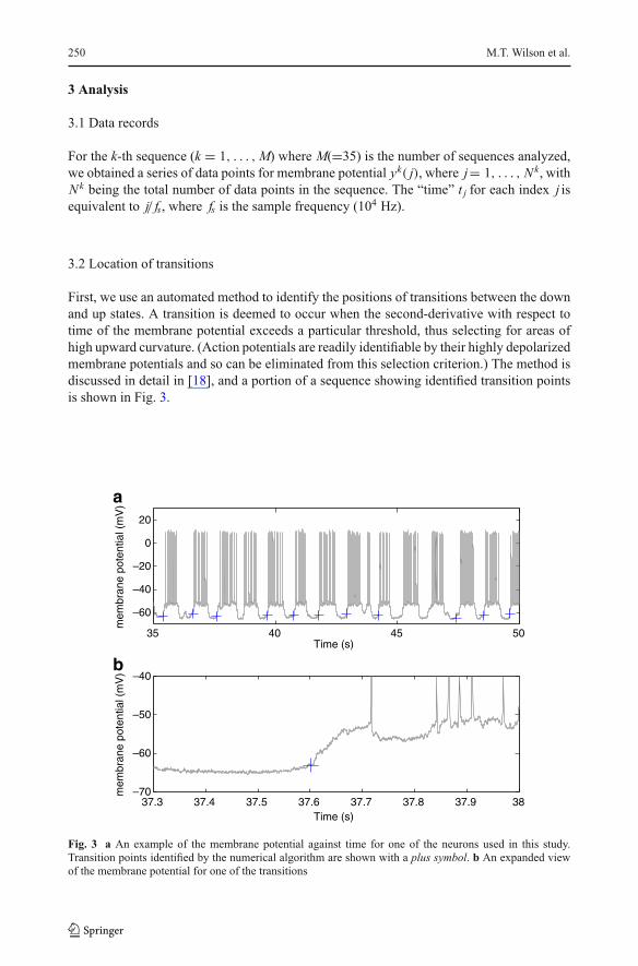
3.2 Location of transitions

First, we use an automated method to identify the positions of transitions between the down

and up states. A transition is deemed to occur when the second-derivative with respect to

time of the membrane potential exceeds a particular threshold, thus selecting for areas of

high upward curvature. (Action potentials are readily identifiable by their highly depolarized

membrane potentials and so can be eliminated from this selection criterion.) The method is

discussed in detail in [18], and a portion of a sequence showing identified transition points

is shown in Fig. 3.

35 40 45 50

–60

–40

–20

0

20

Time (s)

mem

bran

e po

tent

ial (

mV

)

a

37.3 37.4 37.5 37.6 37.7 37.8 37.9 38–70

–60

–50

–40

Time (s)

mem

bran

e po

tent

ial (

mV

)

b

Fig. 3 a An example of the membrane potential against time for one of the neurons used in this study.

Transition points identified by the numerical algorithm are shown with a plus symbol. b An expanded view

of the membrane potential for one of the transitions

Transitions in the cortical slow oscillation 251

Specifically, we define the first and second derivatives d(1)k( j) and d(2)k( j), respectively,

at the point j as:

d(1)k( j) = fs51

(1

50

50∑l=1

yk( j+ l) − 1

50

50∑l=1

yk( j− l)

), (1)

d(2)k( j) = fs101

(1

100

100∑l=1

d(1)k( j+ l) − 1

100

100∑l=1

d(1)k( j− l)

). (2)

In effect, we smooth over 50 time points on either side of the point jfor the first derivative,

and 100 time points for the second. The resulting second derivative is then thresholded at

12,500 mV s−2

, and the points where d(2)kincreases through the threshold are selected as

transition points T kj . For each sequence k, the transition points occur at the indices j= T k

i ,

where i = 1, . . . Pk, with Pk

being the number of transitions in the kth sequence. In this

study, Pkranged from 17 to 78, with a mean value of 52. The exact form of (1) and (2),

along with the choice of threshold, was set after an optimization of the curvature method

of finding a down-to-up transition. The basis was to find a method that maximized the

number of identified transitions but with the constraint that the rate of mis-identification

was extremely low.

3.3 Shape of transitions

The shape of a transition, that is, the trajectory by which the membrane potential moves

from the down to the up state, can be complicated by the presence of action potentials

in the up state. These were removed by identifying spikes through applying a threshold

to the sequences at −30 mV, and removing a short region of data on either side of where

the sequence crosses this threshold. Specifically, the region before the upward crossing of

the threshold where d(1)k > 500 mV s−1

was removed, and the region after the downward

crossing where d(1)k < −200 mV s−1

was removed. A linear interpolation was then applied

across the regions of missing data. Although crude, this approach does not affect the results,

since we only present averaged values for the membrane potential in the up states.

For each sequence k, the transitions were time-aligned, and the average membrane

potential yk( j) was taken over the 0.25-s period (i.e., 2,500 data points) preceding and

the 0.5-s period (i.e., 5,000 data points) following the transition point to produce a mean

transition shape. That is, we evaluated:

yk( j) = 1

Pk

Pk∑i=1

yki( j), (3)

where the sequence yki( j) is given by:

yki( j) = yk(Tki − 2,500 + j) j= 1, . . . 7,500. (4)

Figure 4 shows examples for three different sequences (neurons). Also plotted are the

standard deviations in yki( j) across the transitions i, to indicate the variability between

transitions within one sequence. In the figures in this paper, we have shown time ranging

from 0.25 s before transition through to 0.5 s after, i.e., a total time space of 0.75 s. We start

the graphs at time = 0 s (i.e., j= 0) so that time = 0.25 s corresponds to the transition.

252 M.T. Wilson et al.

0 0.1 0.2 0.3 0.4 0.5 0.6 0.7–90

–80

–70

–60

–50

Time (s)

Pot

entia

l (m

V)

0 0.1 0.2 0.3 0.4 0.5 0.6 0.7–90

–80

–70

–60

–50

Time (s)

Pot

entia

l (m

V)

c

0 0.1 0.2 0.3 0.4 0.5 0.6 0.7–90

–80

–70

–60

–50

Time (s)

Pot

entia

l (m

V)

a

b

Fig. 4 a–c The average transition shape, averaged over all identified transitions from three different neurons.

The central solid line represents the mean membrane potential; the upper and lower dashed lines indicate the

spread in the data by showing one standard deviation higher and lower than this value. The 0.75 s segments

of data have been time-aligned so that the identified transition points, where the down state finishes, occur at

0.25 s

The size and shape of the mean transition across different sequences is somewhat

variable from sequence to sequence, but reasonably constant within a sequence. This may

be a consequence of differing levels of slow-wave sleep being experienced by the animals

in the different experiments. In Fig. 5, we show the mean transition shape yk, and its first

derivative d(1)k, for k = 1, · · · 35, i.e., all neurons of this study. We also identify the position

of each action potential with respect to the transition point, and in Fig. 6, we present a

histogram of the number of action potentials over all the identified up–down transitions

in all the neuron sequences, recorded against time. The distribution of action potentials

across the up state (Fig. 6) has also been examined by Kerr et al. [29]. In that study, action

potentials were found to be uniformly distributed across the up state. Our results are in

broad agreement; for the large majority of the up state, this is true; however, we are able to

resolve the rapid initial rise in the probability of an action potential as the state commences.

Transitions in the cortical slow oscillation 253

0 0.1 0.2 0.3 0.4 0.5 0.6 0.7 0.8–90

–80

–70

–60

–50

–40

Time (s)

Pot

entia

l (m

V)

0 0.1 0.2 0.3 0.4 0.5 0.6 0.7 0.8–400

–200

0

200

400

600

Time (s)

Firs

t Der

ivat

ive

(mV

/s)

a

b

Fig. 5 Color online. a The mean membrane potential and b the mean gradient in the membrane potential

for all the 35 neurons of this study. Each of the 35 thin lines represents the average over all transitions of a

single neuron; the dark, think line represents the mean of these over all these 35 neurons

Figure 5 shows that, after the averaging over all sequences, there appears a clear

oscillation at frequency 50 Hz, particularly on the lower, gradient graph (b). This is

attributed to an artifact of the method used to find the first and second derivatives; such

a scheme, involving forward and backward averaging over a number of points, emphasizes

Fig. 6 The number of spikes

recorded for a given time past the

point of transition, summed over

all identified transitions in all

neuron sequences. The points of

transition have been time-aligned

to 0.25 s

0 0.1 0.2 0.3 0.4 0.5 0.6 0.70

20

40

60

80

100

120

140

160

time (s)

num

ber

of s

pike

s

254 M.T. Wilson et al.

any 50-Hz component that is present in the signal. We do not consider this oscillation to

be of significance. To test for sensitivity of our results to changes in processing method,

we made small changes to the parameters of our analysis; the results were not significantly

changed.

We now focus on the shape of the transition. Figure 5 clearly indicates a sharp rise

in membrane potential in the early stages of the transition—as the membrane potential

rises, its gradient reduces. Figure 6 demonstrates a corresponding increase in frequency

of action potentials. This effect has been quantified by looking at the time-difference

between the maximum gradient in membrane potential and the “halfway” point of the

transition. Specifically, for each transition i in each sequence k, the time of the peak of

the first derivative, t kmax,i, and the time-centroid of the plot of gradient against time, t k

c,i,

were identified. The difference between the two is a measure of how early in the course of

the transition the peak gradient occurs—i.e., how sudden is the transition’s onset? That is,

we constructed the quantities:

�t ki = t k

max,i − t kc,i, (5)

where

t kc,i =

∑T ki +R

j=T ki −R d(1)k( j)t j∑T k

i +Rj=T k

i −R d(1)k( j), (6)

and t kmax,i is the time at which the maximum value of d(1)k

occurs for the ith transition of

the kth sequence, with R = 2,500 (= fs × 0.25 s) denoting 0.25 s on either side of the

transition and t j the time index of the jth data point (= j/ fs). The timing of the peak of

the first derivative d(1)kis denoted by t k

max,j.

A histogram of the values of �tki for all transitions in all sequences is shown in Fig. 7.

It is clear from the figure that the maximum derivative usually occurs before the “halfway

point” of the transition, indicating that the movement of membrane potential away from the

down state is more sudden than its arrival in the up state.

Fig. 7 A histogram of the

difference between time of

maximum gradient in membrane

potential and centroid of the plots

of the gradient against time (i.e.,

the difference between the peak

and the time-centroid of the plots

of gradient of membrane

potential against time). The

distribution is skewed towards

negative values, indicating that

the maximum gradient occurs

early in the transition

–0.4 –0.3 –0.2 –0.1 0 0.1 0.2 0.3 0.40

10

20

30

40

50

60

70

80

Time offset of maximum gradient (s)

Fre

quen

cy

Transitions in the cortical slow oscillation 255

Fig. 8 A histogram of neuron

time constants obtained by fitting

an exponential response to the

membrane potential following

the point of transition from a

down to up state

0 0.05 0.1 0.15 0.2 0.250

1

2

3

4

5

6

7

8

9

10

response time (s)

num

ber

of n

euro

ns

Although there is variation in transition shape, most of the curves of Fig. 5 show an

exponential approach to the up state following the transition point. By fitting an exponential

function of form yk(s) = Ak − Bkexp(−s/t∗k) to the region where time s > 0, where Ak

and

Bkare constants and t∗k

are time constants, we can obtain a distribution of time constant t∗k

for the neurons. This distribution is shown in Fig. 8; the range of time constants is broadly

50 to 150 ms. Although not directly comparable, the analysis of Cossart et al. [21] for the

down to up transition involved with cognition obtained a mean value of 58 ms with standard

deviation 5 ms, which is of similar magnitude to our results. There can be many time scales

that contribute towards the dynamics of the membrane potential; however, it is reasonable

to compare this scale with time scales used in the modelling of membrane potential in

brain dynamics studies. Indeed, our range of time constants is typical of that used in neural

modelling. For example, Bojak and Liley allowed the somatic time constants to range from

5 to 150 ms [30] and Steyn-Ross et al. have used 50 ms [31]. We find that the time constants

Fig. 9 A plot of neuron time

constant against the mean

membrane potential of the down

state at the point of transition, for

each neuron of this study. The

line denotes a least squares linear

fit to the data. There is a clear

negative correlation; neurons

with the more hyperpolarized

down states have the largest

time constants

–90 –85 –80 –75 –70 –65 –600

50

100

150

200

250

Membrane potential in down state (mV)

Tim

e sc

ale

(ms)

256 M.T. Wilson et al.

are correlated with the membrane potential of the down state (R = −0.47, with a probability

of obtaining such a correlation assuming uncorrelated variables as p = 0.0047), presumably

because of changes in potassium channel conductance in the down state. Figure 9 shows

that the neurons with the most hyperpolarized down states are the ones with the largest

time constants—i.e., ones that respond most slowly. It is interesting to note that these time

scales are rather longer than those found by Fuentealba et al. for thalamic reticular neurons

(48 ms) [10], suggesting that the thalamus would respond more quickly to a depolarizing

event.

4 Discussion

Although individual down-to-up transitions are fairly variable in shape, the mean transition

shape for each neuron shows similar features. Specifically, the membrane potential slowly

rises on the approach to the transition, and then undergoes a sudden increase in gradient,

driving it towards a more depolarized state. As the membrane depolarizes, the gradient

reduces, until it settles into a roughly constant up state, where action potentials may form

depending upon the extent of the depolarization.

The trajectory takes on a broadly exponential form. The fast movement of the membrane

potential away from the down state is not what would be expected as a result of critical

slowing on the approach to a first-order phase transition. Rather, we would expect a slow

initial movement away from the ghost of the down state [23]. The exponential trajectory is

equivalent to, for example, the response of the potential difference over the capacitor of a

resistor–capacitor (RC) circuit to a step-change in input voltage. Such a response suggests

that the up and down states experienced by the neurons of this study are merely a passive

response to a step-like switch in synaptic (or other) input, possibly from the thalamus.

Fuentealba et al. indicate a switching time of order 50 ms for the natural switching of the

bistability in reticular cells of the thalamus [10]; this is faster that the response of most

of the cortical cells of this study. This indicates that the thalamic input to the cortical cells

might be broadly considered step-like on the time scale of the cortical cells. The observation

of Wilson et al. [18] that the power spectrum of fluctuations in membrane potential on

the approach to a transition decays approximately as 1/ f 2, where f is frequency, is also

consistent with the hypothesis of the cortical neuron acting like an RC circuit; an input of

a broad spectral nature (e.g., as a result of an approximately white noise source) to an RC

circuit, or indeed to any linear system [32], would be expected to give rise to a spectrum

that decays as 1/ f 2.

The correlation between the time constant and the membrane potential of the down state

(Fig. 9) is consistent with the fact that membrane input resistances in the up state (ap-

proximately 9 M�) are much lower compared with those of the down state (approximately

40 M�), by around a factor of four [33, 34]. In terms of the RC circuit model, where the time

constant is given by RC, this would mean that a hyperpolarized neuron has four times the

time constant compared to when it is depolarized. If we assume that the input resistance

varies approximately smoothly between the extremes, we may expect a greater time

constant for the most hyperpolarized neurons. The range that we see in Fig. 9, namely,

about a threefold reduction in time constant for a −60-mV down state as opposed to a

−90-mV down state, is broadly consistent with the measurements of input resistance. The

power surge and slowing of fluctuations that are demonstrated in the neurons studied in [18]

Transitions in the cortical slow oscillation 257

could then be considered purely as a response of these neurons to a power surge and critical

slowing in a system feeding these cortical neurons.

These results therefore suggest that, while a first-order phase transition may be an

underlying driver of the cortical slow oscillation, the phase transition is not entirely located

in the cortical neurons themselves. This is in contrast with the result of Sanchez-Vives

and McCormick, who found that the slow oscillation in vitro in ferret neocortex appeared

first in layer 5 [14]. (Note that layer 5 neurons were included in our study.) Given the

relatively short time scales for onset of depolarization in reticular thalamic neurons [10],

which can be viewed as quick compared with the cortical neurons, one could speculate

that the initiation of the up state in the cortex is merely a response to a fast change in

the thalamus. Alternatively, given evidence that there is a cortical component to the slow

oscillation [7], one could speculate that the dynamics may be more complicated than a

simple picture can represent: the slow oscillation is neither a collective mode of the cortex

(as the phase transition model would predict), nor a response in individual cortical neurons

to an underlying oscillation elsewhere in the brain. A hybrid mode, combining the two

extremes, may be more appropriate. Such a picture would be consistent with the results of

Kerr et al. [29], who have determined, through the use of voltage-sensitive dyes, that the

active population of neurons is constantly changing, that is, “pacemaker” ensembles might

be dynamic in the cortex and thalamus. For example, initiation might be in layer 5 [14], but

only in a small subset of neurons. From this study, it is not possible to make a definitive

statement on the origin of the slow oscillation, other than to remark that it did not appear to

be entirely located within the neurons studied. There are many possibilities that remain. It is

therefore plausible that a similar experimental analysis of membrane potential fluctuations

in thalamic cells, either in vivo or in vitro, might shed light on the origin and maintenance

of the slow oscillation.

Analysis of the data is complicated by the need to define where a transition takes place.

In essence, by using a method based on curvature of the membrane potential, we have

implicitly assumed that transitions are sudden, and that may bias our results. In fact, merely

assuming that a “transition” occurs might be biasing results in favor of a sudden initial

jump. However, an examination by eye suggests that one can define a transition point at

least loosely, and the analysis is robust to small changes in parameters. Moreover, we have

selected the neurons for this study on the grounds that they gave clearly distinguishable

down and up states. This itself may introduce bias into the study—e.g., emphasize the

suddenness of a transition between the states. If that were the case, however, one would

still expect the conclusions to hold for those particular neurons, which are a significant

subset of those recorded.

Finally, we must remark that the data have been recorded from animals under urethane

anaesthesia, not from naturally sleeping animals. The mechanisms by which the up and

down states are generated during anaesthesia may not be identical to that of natural sleep.

The electroencephalograms of naturally sleeping and urethane-anaesthetized rats have been

compared by Clement et al. who found no major differences between the two and concluded

that urethane anaesthesia is a good model of sleep in rats [35]. Additionally, Sceniak and

MacIver found that the mechanism of urethane action on rat visual cortical neurons in vitrowas activation of a K

+leak current, as opposed to modulation of synaptic transmission; this

is similar to natural sleep [36]. However, one should not make the general conclusion that

urethane anaesthesia and natural slow-wave sleep are the same state; for example, the down

states in anaesthetized cats [1] are longer than those in naturally sleeping animals [37].

258 M.T. Wilson et al.

5 Conclusion

In this paper, we have looked at the dynamics in the membrane potential of the transition

between the down and the up states of the cortical slow oscillation. The transition shows

characteristics broadly similar to that of a simple RC circuit. This is not consistent with

the hypothesis that the transition is a result of a phase transition within single cortical

neurons, or large assemblies of cortical neurons. Rather, results are suggestive of the cortical

neurons that were measured being driven by step-like changes in input. It is still possible,

or even likely, given the evidence from the changes in power spectrum at the transition

point [18], that there exists an underlying phase transition, either in the thalamus, or in a

small subset of cortical cells, or some combination of the cortex and thalamus. Alternatively,

the brain dynamics causing and maintaining the oscillation may be more complicated still,

for example, a hybrid of collective and individual neural modes.

Acknowledgement The authors would like to thank Peter Robinson of the University of Sydney for helpful

discussions.

References

1. Steriade, M., Núnez, A., Amzica, F.: A novel slow (<1 Hz) oscillation of neocortical neurons in vivo:

depolarizing and hyperpolarizing components. J. Neurosci. 13, 3252–3265 (1993)

2. Marshall, L., Helgadóttir, H., Mölle, M., Born, J.: Boosting slow oscillations during sleep potentiates

memory. Nature 444, 610–613 (2006)

3. Tononi, G., Cirelli, C.: Sleep function and synaptic homeostatis. Sleep Med. Rev. 10, 49–62 (2006)

4. Destexhe, A.: Self-sustained asynchronous irregular states and up-down states in thalamic, cortical

and thalamocortical networks of nonlinear integrate-and-fire neurons. J. Comput. Neurosci. (2009).

doi:10.1007/s10827-009-0164-4

5. Compte, A., Sanchez-Vives, M.V., McCormick, D.A., Wang, X.J.: Cellular and network mechanisms of

slow oscillatory activity (<1 Hz) and wave propagations in a cortical network model. J. Neurophysiol.

89, 2707–2725 (2003)

6. Hill, S., Tononi, G.: Modeling sleep and wakefulness in the thalamocortical system. J. Neurophysiol. 93,

1671–1698 (2005)

7. Steriade, M., Núnez, A., Amzica, F.: Intracellular analysis of relations between the slow (<1 Hz)

neocortical oscillation and other sleep rhythms of the electroencephalogram. J. Neurosci. 13, 3266–3283

(1993)

8. Timofeev, I., Grenier, F., Bazhenov, M., Sejnowski, T.J., Steriade, M.: Origin of slow cortical oscillations

in deafferated cortical slabs. Cerebral Cortex 10, 1185–1199 (2000)

9. Blethyn, K.L., Hughes, S.W., Tóth, T.I., Cope, D.W., Crunelli, V.: Neuronal basis of the slow (<1 Hz)

oscillation in neurons of the nucleus reticularis thalami in vitro. J. Neurosci. 26, 2474–2486 (2006)

10. Fuentealba, P., Timofeev, I., Bazhenov, M., Sejnowski, T., Steriade, M.: Membrane bistability in thalamic

reticular neurons during spindle oscillations. J. Neurophysiol. 93, 294–304 (2005)

11. Wilson, M.T., Steyn-Ross, D.A., Sleigh, J.W., Steyn-Ross, M.L., Wilcocks, L.C., Gillies, I.P.: The

k-complex and slow oscillation in terms of a mean-field cortical model. J. Comput. Neurosci. 21, 243–

257 (2006)

12. Massimini, M., Huber, R., Ferrarelli, F., Hill, S., Tononi, G.: The sleep slow oscillation as a traveling

wave. J. Neurosci. 24, 6862–6870 (2004)

13. Bazhenov, M., Timofeev, I., Steriade, M., Sejnowski, T.J.: Model of thalamocortical slow-wave sleep

oscillations and transitions to activated states. J. Neurosci. 22, 8691–8704 (2002)

14. Sanchez-Vives, M.V., McCormick, D.A.: Cellular and network mechanisms of rhythmic recurrent

activity in neocortex. Nat. Neurosci. 3, 1027–1034 (2000)

15. Amzica, F., Steriade, M.: The functional significance of the k-complexes. Sleep Med. Rev. 6, 139–149

(2002)

16. Molaee-Ardekani, B., Senhadji, L., Shamsollahi, M.B., Vosoughi-Vahdat, B., Wodey, E.: Brain activity

modeling in general anesthesia: enhancing local mean-field models using a slow adaptive firing rate.

Phys. Rev. E 76, 041911 (2007)

Transitions in the cortical slow oscillation 259

17. Robinson, P.A., Wu, H., Kim, J.W.: Neural rate equations for bursting dynamics derived from

conductance-based equations. J. Theor. Biol. 250, 663–672 (2008)

18. Wilson, M.T., Barry, M., Reynolds, J.N.J., Hutchison, E.J.W., Steyn-Ross, D.: Characteristics of temporal

fluctuations in the hyperpolarized state of the cortical slow oscillation. Phys. Rev. E 77, 061908 (2008)

19. Steyn-Ross, D.A., Steyn-Ross, M.L., Sleigh, J.W., Wilson, M.T., Gillies, I.P., Wright, J.J.: The sleep

cycle modelled as a cortical phase transition. J. Biophys. 31, 547–569 (2005)

20. Steyn-Ross, D.A., Steyn-Ross, M.L., Wilson, M.T., Sleigh, J.W.: White-noise susceptibility and critical

slowing in neurons near spiking threshold. Phys. Rev. E 74, 051920 (2006)

21. Cossart, R., Aronov, D., Yuste, R.: Attractor dynamics of network up states in the neocortex. Nature 423,

283–288 (2003)

22. Wilson, M.T., Steyn-Ross, M.L., Steyn-Ross, D.A., Sleigh, J.W.: Predictions and simulations of cortical

dynamics during natural sleep using a continuum approach. Phys. Rev. E 72, 051,910 1–14 (2005)

23. Strogatz, S.H.: Nonlinear Dynamics and Chaos. Westview, Cambridge (2000)

24. Chagnac-Amitai, Y., Luhmann, H.J., Prince, D.A.: Burst generating and regular spiking layer 5 pyrami-

dal neurons of rat neocortex have different morphology features. J. Comp. Neurol. 296, 598–613 (1990)

25. Steriade, M.: Corticothalamic resonance, states of vigilance and mentation. Neuroscience 101, 243–276

(2000)

26. Brecht, M., Krauss, A., Muhammed, S., Sinai-Esfahani, L., Bellanca, S., Margrie, T.W.: Organization

of rat vibrissa motor cortex and adjacent areas according to cytoarchitectonics, microstimulation, and

intracellular stimulation of identified cells. J. Comp. Neurol. 479, 360–373 (2004)

27. Games, K.D., Winer, J.A.: Layer V in rat auditory cortex: projections to the inferior colliculus and

contralateral cortex. Hear. Res. 34, 1–25 (1988)

28. Reynolds, J.N.J., Hyland, B.I., Wickens, J.R.: Modulation of an afterhyperpolarization by the substantia

nigra induces pauses in the tonic firing of striatal cholinergic interneurons. J. Neurosci. 24, 9870–9877

(2004)

29. Kerr, J.N.D., Greenberg, D., Helmchen, F.: Imaging input and output of neocortical networks in vivo.

Proc. Natl. Acad. Sci. 102(39), 14063–14068 (2005)

30. Bojak, I., Liley, D.T.J.: Modeling the effects of anaesthesia on the electroencephalogram. Phys. Rev. E

71, 041902 (2005)

31. Steyn-Ross, M.L., Steyn-Ross, D.A., Wilson, M.T., Sleigh, J.W.: Modeling brain activation patterns for

the default and cognitive states. NeuroImage 45, 289–311 (2009)

32. Hutt, A., Frank, T.D.: Critical fluctuations and 1/ f α-activity of neural fields involving transmission

delays. Acta Phys. Pol., A 108, 1021–1040 (2005)

33. Destexhe, A., Paré, D.: Impact of network activity on the integrative properties of neocortical pyramidal

neurons in vivo. J. Neurophysiol. 81, 1531–1547 (1999)

34. Destexhe, A., Rudolph, M., Paré, D.: The high-conductance state of neocortical neurons in vivo. Nat.

Rev. Neurosci. 4, 739–751 (2003)

35. Clement, E.A., Richard, A., Thwaites, M., Ailon, J., Peters, S., Dickson, C.T.: Cyclic and sleep-like

spontaneous alternations of brain state under urethane anaesthesia. PLoS ONE 3, e2004 (2008)

36. Sceniak, M.P., MacIver, M.B.: Cellular actions of urethance on rat visual cortical neurons in vitro. J.

Neurophysiol. 95, 3865–3874 (2006)

37. Steriade, M., Timofeev, I., Grenier, F.: Natural waking and sleep states: A view from inside neocortical

neurons. J. Neurophysiol. 85, 1969–1985 (2001)