i

Acknowledgements

I would like to thank my supervisor Mr H. Nare for the constant guidance that he provided during

the writing of this dissertation.

I would like to thank my family, in particular my mother and little sister (M. Sihwa and P. Sihwa),

for their constant encouragement and support. I would also like to thank my friends for the support

and understanding that they showed me.

Finally, a special thanks goes to my Lord and savior Jesus Christ without whom my existence

would be unworthy while.

ii

Abstract This paper explores and compares the effects of five macro-econometric variables on the volume

of manufacturing index (VMI) from January 2009 to December 2014. In particular we investigate

the return causality relationships by applying vector auto-regressive analysis. This paper also

analyses the differences in model building using stationary data that has been differenced to

achieve stationarity and model from non-stationary data given that the variables are cointegrated.

The empirical findings indicate that some variables namely,

Exchange rate, money supply, product demand, and interest rate have an effect on the future values

of VMI. I discovered that at most two equations were cointegrated meaning that macro-

econometric variables are cointegrated with VMI in the long run. The effect of some government

policies on VMI were measured using impulse response analysis for both the VAR and VEC

model. Overall compared to the VAR model, the VEC model proved to be supreme in terms of

forecasting power.

iii

Contents Abstract ......................................................................................................................................................... ii

CHAPTER ONE ........................................................................................................................................... 1

1.1 Introduction ................................................................................................................................. 1

1.1.2 Background of Study ................................................................................................................. 1

1.2 Problem Statement ............................................................................................................................ 3

AIM .......................................................................................................................................................... 4

Objectives................................................................................................................................................. 4

1.2.1 Research Questions .................................................................................................................... 5

1.3 Significance of the study ................................................................................................................... 5

1.4 Limitations ......................................................................................................................................... 5

1.4.1 Delimitations ............................................................................................................................... 6

CHAPTER TWO .......................................................................................................................................... 7

2.1 Introduction ....................................................................................................................................... 7

2.1.1 Economic benefits arising from a well performing manufacturing sector ........................... 7

2.1.2 Case of the Nigeria Industry ..................................................................................................... 8

2.1.3 Phenomenon of interdependence .............................................................................................. 9

2.1.4 United States industry sector .................................................................................................... 9

2.2 Vector Autoregressive Model ......................................................................................................... 10

2.2.1 Application of VAR model: Pakistan manufacturing sector index (1976-2001). ............... 11

2.3 Impulse Response Functions (IRF) ............................................................................................... 13

2.4 Vector Error Correction Model ..................................................................................................... 13

2.4.1 A Vector Error Correction Model (VECM) Approach in Explaining the Relationship

between Interest Rate and Inflation towards Exchange Rate Volatility in Malaysia. ................ 14

CHAPTER THREE .................................................................................................................................... 16

3.1 Methodology .................................................................................................................................... 16

3.1.1 Nature and sources of data ...................................................................................................... 17

3.2 Selection of Variables ..................................................................................................................... 17

Manufacturing Output ......................................................................................................................... 17

1. Money supply (M3) ................................................................................................................... 18

2. Interest Rates (Intr) .................................................................................................................. 18

3. Exchange rates (EX) ................................................................................................................. 18

4. Labor cost (LC) ......................................................................................................................... 19

iv

5. Product demand (PD) ............................................................................................................... 19

3.2.1 Data Exploration ...................................................................................................................... 20

3.3 Lag Selection.................................................................................................................................... 20

Akaike Information Criterion .......................................................................................................... 20

Schwartz information criterion ....................................................................................................... 21

3.4 Selection of variables to include in the model ............................................................................... 21

3.4.1 Granger Causality test ............................................................................................................. 21

3.5 VAR Model Formulation................................................................................................................ 22

3.6 Model Evaluation and diagnostics ................................................................................................. 23

3.6.1 Durbin Watson h test ............................................................................................................... 23

3.6.2 Augmented Dickey Fuller test ................................................................................................. 24

3.7 Analysis of Residuals ...................................................................................................................... 25

3.7.1 Goodness to fit test ................................................................................................................... 25

3.8 Impulse Response Functions to policy shocks .............................................................................. 25

3.8.1 ZIM-ASSET POLICY ............................................................................................................. 26

3.9 VEC Model Building ....................................................................................................................... 27

3.9.1 Johansen Test ........................................................................................................................... 27

3.10 VEC model formulation ........................................................................................................... 28

3.11 Conclusion ..................................................................................................................................... 29

CHAPTER FOUR ....................................................................................................................................... 30

Data Analysis, Inference and Interpretation of Results .............................................................................. 30

4.1 Introduction ..................................................................................................................................... 30

4.1.1 Data Exploration ...................................................................................................................... 30

4.2 Lag Length Selection ...................................................................................................................... 31

4.3 Granger Causality Test .................................................................................................................. 32

4.3 VAR Model formulation. ................................................................................................................ 33

4.4. Model Appropriateness ................................................................................................................. 35

4.4.1 Durbin Watson ............................................................................................................................. 35

4.4.2 Normality test ........................................................................................................................... 35

4.5 Impulse Response Functions .......................................................................................................... 36

4.5.1 Impulse response due to Funding and Debt Management (Strategy). ................................ 36

4.5.2 Impulse Response due to Value Addition and Beneficiation. (Cluster) .............................. 37

4.6 Forecasting using developed VAR Model ..................................................................................... 39

v

4.7 VEC model Building ....................................................................................................................... 40

4.7.1 Johnsen Cointegration Test ..................................................................................................... 40

4.8 VEC Model Formulation ................................................................................................................ 40

4.9 Model Appropriateness .................................................................................................................. 42

4.9.1 Durbin Watson ......................................................................................................................... 42

4.9.2 Normality Test .......................................................................................................................... 42

4.10 Impulse Response Functions Using VEC Model ........................................................................ 43

4.10.1 Impulse response due to Funding and Debt Management (Strategy). .............................. 43

4.10.2 Impulse Response due to Value Addition and Beneficiation. (Cluster) ............................ 44

4.11 Forecasting using developed VEC Model ................................................................................... 46

4.12 Comparison of Models in their Forecasting power .................................................................... 47

4.13 Conclusion ..................................................................................................................................... 47

4.14 Forecast for 2015 Using VEC Model ........................................................................................... 48

CHAPTER FIVE ........................................................................................................................................ 49

5.1 Conclusion and Recommendations................................................................................................ 49

5.1.1 Conclusions drawn from the study ......................................................................................... 49

5.2 Recommendations ........................................................................................................................... 50

References ................................................................................................................................................... 51

Appendix ..................................................................................................................................................... 54

vi

List of Figures

Figure 1. Summary of steps in chapter three.

Figure 2a. TS-Plot for volume of manufacturing index.

Figure 2b. TS-Plot for first difference of volume of manufacturing index.

Figure 3a. Response of VMI to a positive shock in Money Supply (M3). (VARM)

Figure 3b. Response of VMI to a positive shock in Product Demand (PD). (VARM)

Figure 4a. Response of VMI due to a positive shock in M3 (VECM)

Figure 4b. Response of VMI due to a positive shock in PD. (VECM).

List of Tables

Table 1. Test for stationarity results.

Table 2. Lag selection Results.

Table 3. Granger Causality Results.

Table 4. Vector Autoregressive model.

Table 5. Durbin Waston Results (VARM).

Table 6. Normality Test Results.

Table 7. VAR model forecast (2014)

Table 8 Jahansen Cointegration Results.

vii

Table 9. Vector Error Correction Model.

Table 10. Durbin Watson test results (VECM)

Table 11. Normality test results (VECM).

Table 12.VEC model forecast. (VECM)

Table 13a. % Error in forecasting power of VARM

Table 13b. % Error in forecasting power of VECM

Table 13c. Comparison of error in forecasting power of VARM and VECM

Table 14. Forecast for Volume of manufacturing for 2015 using the developed VEC model

1

CHAPTER ONE

1.1 Introduction

This chapter highlights the background of the study to be conducted, the problem statement

which will fully explain the need for the project to be conducted in the first place. The aim of the

project and the various objectives which are meant to be achieved are also outlined. As in any

project limitations are not to be ignored and hence will be included in this chapter.

1.1.2 Background of Study

As Zimbabwe moves forward, there is an urgent need to put in place economic strategies that

will steer the country into a better tomorrow. In order to be able to put these strategies in place

econometric models should be developed to allow us to be able to forecast future outcomes and

thereby establishing policies to manage the predicted outcomes. Econometric models are

therefore developed to explain, interpret, test hypothesis of interest, forecast and take policy

actions relative to the economic situation of interest (Young, R.M. and Klein, L.R. 2006).Before a

meaningful conclusion can be made, we have to be sure that the model describes the data

sufficiently.

Zimbabwe has experienced a deteriorating economic environment since 2000 (CZI in-house

magazine 2011). This resulted in a major economic crisis characterized by industrial capacity

utilization of below 10% and an overall cumulative Gross Domestic product (GDP) decline of

50% by 2008 (ZIMSTAT economic review 2009). The Zimbabwean government in 2009

introduced some measures for economic stabilization which saw Zimbabwe achieving a real

GDP growth rate of 5.4% in 2009, 11.4% in 2010 and 11.9% in 2011.Recovery of the economy

remained strained as growth rate declined from 11.9% in 2011 to 10.6% in 2012 and 3.4% in

2013 (ZIMASSET policy document 2013).

The trade and manufacturing sector plays an important role in the economy of Zimbabwe, it

contributes significantly to gross domestic output, export earnings and employment. It is key to

2

the economic development of Zimbabwe because it stimulates economic growth and job creation

through the development of micro, small and medium Enterprises. The broadly based

manufacturing sector produces in excess of 6,000 products or commodities ranging from food and

clothing to fertilizers and chemicals, metal products of all kinds, electrical machinery and

equipment and motor vehicle assembly. The manufacturing industry is closely linked to agriculture

with an excess of 60% of manufacturing value added either related to agro-industry or to the

provision of inputs to the agricultural sector.

The manufacturing sector however remains a crisis with capacity utilization declining from an

average 57% in 2011, 44% in 2012 and 39% in the 3rd quarter of 2013 (Zimbabwe industrial

development policy 2011-2015). These declines were attributed to structural and infrastructural

challenges such as unpredictable power supply, old machinery and infrastructure and lack of and

high cost of capital (Muponda, G.2013). According to the ZIMASSET document, Zimbabwe is

projected to be a growth leader in Sub-Saharan Africa towards 2020 and since the manufacturing

sector is a major contributor to GDP it is of paramount importance to analyze the impact of the

major variables that contribute to its growth however the countries capacity utilization level

continues to decline and it seem it will continue in this trend due to a number of factors. Finance

minister Patrick Chinamasa, in his 2015 budget presentation said the sector was expected to

register a marginal growth of 1.7%, hinged on sustained implementation of supportive policy

interventions highlighted in the 2014 Mid-Year Fiscal policy statement (Zimbabwe Independent,

Dec 2014). The Ministry of Industry and Commerce is mandated to create a vibrant self-sustaining

and competitive economy through promotion of viable industrial and commercial sectors as well

as increasing domestic and international trade hence models have to built to assist in policy

formulation.

The government has introduced a number of policies which are trying to make conditions

conducive for increase in capacity, one of the famous policies introduced is the Zimbabwe Agenda

for Sustainable Socio-Economic Transformation (ZIMASSET). Future effects of such policies

have to be studied and appropriate adjustments made.

3

1.2 Problem Statement

The world is shrinking day by day with the advancement of technology. The expectations of human

beings are rising. Economic liberalization is finding greater roots. Globalization of the economy

is becoming a worldwide phenomenon. It is, however established that survival and economic

growth of any country will depend on increase of productivity. This is particularly important in

developing countries, Zimbabwe included because of higher population growth, declining GDP,

growing debt, higher interest burden, domestic and international competition, scarcity of raw

materials, balance of payment problem, fiscal deficit etc. Some of these problems can be overcome

by paying greater attention to managing productivity especially in the manufacturing sector.

Decrease in industrial production has resulted in many jobs getting shed, a situation that has

resulted in significant ripple effect through related service industries.

The major constraints to capacity remain largely unchanged with government failing to address

the fundamentals needed to attract the much needed investment. Though the contributing variables

have been identified and some policies implemented, the problem lies in the limitations of the

methods used. The methods used identify each variable separately and a corresponding policy is

put in place to deal with this. Professor Mutambara (The Standard, 2013) highlighted that currently

issues are being addressed using a single variable approach, which is a weak approach. A better

approach would be to identify the interdependence of the variables and the extent to which changes

in each affects the other and in turn the levels of capacity utilization so as to be able to manipulate

the variables to improve capacity. To address this problem a different approach to model building

will be taken by looking at models using stationary data and non-stationary data.

VAR models have been widely used in econometrics to investigate the characteristics and

changes in key macro econometric variables. VAR models have been used for Policy evaluation

and have also been shown to provide good forecast. Although VAR models have their

advantages, they are computational demanding and when restrictions are imposed on them i.e.

differencing, so as to achieve stationarity, large numbers of data have to be thrown out and hence

leading to significant inadequacy and inefficiency of the developed model.

4

The finding that many macro time series data may contain a unit root (non-stationary) has led to

the proposal of a model to be developed using non-stationary data that is cointegrated.

Restrictions will be imposed on the VAR model so that the modified model is locally stationary

and has bounded mean. To do this the Vector Error Correction model will be developed using

non-stationary data. The VEC model is a restricted VAR model that has cointegration restrictions

built into the specification so that it is specially designed for use with non-stationary data. The

model will allow non-stationary variables to be in the equation and forecast will be done using

the developed model.

AIM

To develop a model that improves on the forecasting power of the Vector Autoregressive model

so as to analyze Zimbabwe’s Manufacturing Sector Index (2009-2014).

Objectives

Describe the relationships between the variables of interest / constraints on the

manufacturing sector using VAR model.

Find the most influential and sensitive constraint to capacity utilization.

Trace the effect of one standard deviation shock to one of the innovations on the future

values of the endogenous variable using the VAR model.

Forecast Volume of Manufacturing Index values for the year 2014 using developed

model.

Impose restrictions on VAR model by developing a Vector Error Correction model so as

to allow non-stationary data to be used in model formulation.

Trace the effect of one standard deviation shock to one of the innovations on the future

values of the endogenous variable using the VEC model.

Forecast Volume of Manufacturing Index for the year 2014 using the VEC model.

Compare forecasting power of the unrestricted VAR model as compared to the VEC

model.

Forecast VMI for the year 2015 using the better model.

5

1.2.1 Research Questions

This study specifically seeks to answer the following research questions.

1. Is there a significant difference in the forecasting power of the VAR model compared to

the VEC model?

2. How are the variable interrelated.

3. Are all variables that are thought to affect VMI theoretically indeed affect VMI in the

way we think they do?

4. Are policy changes within the economy explainable using the models developed?

5. By what factor does Volume of Manufacturing Index increase in the near future?

1.3 Significance of the study

This study is meant to capture the differences between the VAR model and the VEC model and

how they affect the forecasting power of the models taking into consideration manufacturing

sector index for 2015. By changing the model from a model developed using stationary data to a

model developed using non-stationary data, we will be able to study how the models behave with

significant loss of data through differencing to achieve stationarity and how the model behaves

when we are able to stop loss of significant data through differencing. The model developed will

be used to analyse how much a shift in the involved variables contributes to capacity utilization

and the extent of adjustment needed to achieve the desired 100 per cent increase to capacity

utilization in the stipulated time frame. By studying the behaviour of the variables we are able to

adjust certain policies that concern the given variables so as to improve capacity utilisation. The

study will help in identifying the most sensitive variable to capacity utilization, by singling out

the variables, we are able to come up with policies that monitor the levels of that particular

variable at a desired level.

1.4 Limitations

Unavailability of data for other variables that could have been added in the study such as

electricity availability and raw material availability.

Lack of a knowledge on the use of advanced software packages to analyze data such as

SAS, STATA etc.

6

There is a considerable amount of non-response and data required adjustments by the

statistics office before utilizing it for effective planning.

1.4.1 Delimitations

To enhance feasibility of the study its scope was limited to only one sector enabling a

more focused study to be carried out.

7

CHAPTER TWO

2.1 Introduction

Various improvements on models have been done to try and improve on the results of the data to

be analyzed. Various papers have been published on these improvements highlighting different

methodologies and approaches to these improvements. This chapter will provide a brief overview

of VAR models, VEC models and an overview of previous studies connected to use of non-

stationary data to build models. An overview of a study of a nation with a well performing

manufacturing sector will be looked at first.

2.1.1 Economic benefits arising from a well performing manufacturing sector

A well performing manufacturing sector entails an increase in domestic production of goods

thereby reducing cost of importation of goods previously being imported, for example the Chinese

economy which is the world’s second largest economy after America has one of the best

manufacturing industries in the world producing electronic goods once imported for outrageous

prices but now being affordable (Chinese small manufactures street journal 2006). An increase in

domestic production also means an increase in exported goods thereby bringing in the much

needed foreign currency. Employment opportunities arise because a boom in the manufacturing

sector results in employment for people of different skill sets to get jobs. A well performing

manufacturing sector means that the contribution of the sector to gross domestic product will also

increase. Since most industries for instance mining and agriculture depend on some of the

manufactured products, the increase in the output has a direct/indirect effect on the performance

of these and other sectors

.

8

2.1.2 Case of the Nigeria Industry

According to Ojo, A.S and Ololade, O.F, (2004), the Nigerian manufacturing industry grew quite

rapidly during 1974-80 period. During this period it was observed that manufacturing value added

recorded an annual average growth rate of about 12 percent. However during the end of the oil

boom, the sharp fall in domestic demand and drastic reduction in the countries input capacity had

a direct and significant impact on the manufacturing sector. One of the indicators of this effect was

found to be the rapid decline of capacity utilisation of the manufacturing sector from the peak of

73 percent in 1981 to under 35 percent in 1995. The low import capacity was also found to be

largely responsible for the then observed low capacity utilisation rates that had characterised

Nigerian manufacturing industry over the past decades. The objectives of the Nigerian study were

to identify and appraise the major policies that had been used to induce local sourcing of industrial

raw material, evaluate whether the extent to which policy induced local sourcing of industrial raw

materials had been made possible to technological accumulation and evaluate the rule of local

sourcing of industrial raw materials as a factor influencing industrial capacity utilisation. The study

was divided into three stages. Firstly, policies targeted at promoting the use of local industrial raw

materials were reviewed and an exploration on how each policy induced use of local raw materials

motivated forms to embark on various types of technological development. In order to for that to

happen, visits to companies were done to elicit positive responses to questionnaires. The

questionnaires focused on management policy. From the questionnaires it was found that relying

on domestic sources of local raw material was imperatively brought about by the local supply base

and enhancement of local value added. Secondly the study analysed the main factors that explained

the extent to local sourcing of industrial raw materials. A linear model was developed. The factors

analysed in the model were, capacity utilisation, technological development and form

characteristics. It was found that technological development, form characteristics and capacity

utilisation affected the extent of local sourcing of raw materials. Thirdly the relationship between

local sourcing of raw materials and industrial capacity utilisation was analysed. It was concluded

that there was a strong relationship between local sourcing of raw materials and industrial capacity

utilisation.

9

2.1.3 Phenomenon of interdependence

It is a relation of variables between its members such that each is mutually dependent on the others.

In an interdependent relationship, participants maybe economically reliant and responsible to each

other (Bordoloi, S.D.2011). Interdependence suggest the prevalence of co-movements within a

sector/market. Presence of such co-movements can be explained using the Vector auto-regression

framework. The phenomenon of interdependence across markets has been the subject of extensive

empirical investigation. Early empirical work includes Grubel (1968), Agrom (1972), Lessard

(1973) and many others. Errunza and Losq (1985) assessed the degree of interdependence for

returns among international stock markets and found that the first moments of equity returns

among the stock markets exhibited a degree of interaction.

2.1.4 United States industry sector

Determination of the interdependence of the US industrial sector was found to be of great

importance in the understanding and pre-dictation of their economic behaviour (Bordoloi,

S.D.2011). The sectors where based on industry groups and ranged from July 1962 to December

2008. Investigation into the dynamic linkages of the sectors within a market was found to be crucial

to everyone involved in the markets e.g. policy makers. In formulation of policies, policy makers

can account for the interdependencies in order to shelter some sectors from harm originating in

other sectors. The US 2008 financial crisis is a catastrophic example as to how the crisis in one of

the market sectors (the housing market) rapidly evolved to a nationwide financial crisis and later

engulfed many countries around the world. The study focused on the interdependence among

seven (7) US industries and explored the dynamic changes of such relationships during peaceful

and volatile periods. In order to identify any changes in the pattern of interdependence during

peaceful and volatile periods, a similar VAR analysis for both the periods in addition to the whole

period was conducted. The data was extracted from US industry division daily returns, the US

stock market returns, the US inflation rate, US gross domestic product, US interest rate and US

employment rate. It was found that the portfolio returns were generally high. The VAR of the daily

returns portfolio showed that the first own lags of the sectors were generally significant. The VAR

results also showed that for full periods the value weighted portfolio for both the peaceful and

10

volatile periods own lags were not significant for most of the divisions and there was no division

which dominantly influenced all the other divisions, only market returns amongst the exogenous

variables significantly affected the division of the industry.

2.2 Vector Autoregressive Model

VAR models are an extension of univariate auto-regression models to time series data. A VAR

model is a multi-equation system where all the variables are treated as endogenous. There is one

equation for each variable as the dependent variable. Right hand side of each equation includes

lagged values of all dependent variables in the system.

VAR-Models themselves do not allow us to make statements about causal relationships within the

data. This holds especially when VAR-Models are only approximately adjusted to an unknown

time series process, while a causal interpretation requires an underlying economic model

(Luetkepohl, H. 2011). However, VAR-Models capture the dynamic relationships between the

indicated k variables (endogenous) over the same time period as a linear function of only the past

values. VAR models make minimal theoretical demands on the structure of the model one only

needs to specify the set of variables that are believed to interact and hence should be included as

part of the economic system that is being modelled and the number of lags that are needed to

capture most of the effects that the variables have on each other.. There are 3 varieties of VAR

models namely Reduced, Structural and Recursive models.

Reduced form- expresses each variable as a linear function of its own past values, past

values of other variables under consideration, and a serially uncorrelated term. Each

equation is determined by Ordinary Least Squares (OLS) regression.

Recursive VAR - constructs error term in each regression equation to be uncorrelated with

the error in the previous equations.

Structural VAR -uses economic theory to sort out same time links between variables (Sim

1986) i.e., variables are not just chosen randomly but those that have proven to have a

relationship with the independent variable are chosen.

11

For a set of time series variables:

Yt = (Y1t, Y2t… Ynt)

a VAR (p) can be written as:

Yt = A + B1Yt-1 + B2Yt-2 + … + BpYt-p + Et

Where:

Yt = (y1t, y2t… ynt)’: an (nx1) vector of time series variables.

A: an (nx1) vector of intercepts.

Bi (i=1, 2… p): (n x n) coefficient matrices.

Et: an (nx1) vector of unobservable i.i.d. zero mean error term (white noise).

VAR models are one of the most successful and flexible models for the analysis of multivariate

time series. They are especially useful for describing the dynamic behavior of economic and

financial time series and are also useful for forecasting. VAR models are used to analyse systems

responses to different shocks / impacts. In economics, VAR models are used to forecast

macroeconomic variables, such as GDP, money supply, and unemployment. When using VAR

models, all data must have to have same frequency and data with mixed frequency must be

converted to the same frequency i.e. monthly, daily or yearly.

2.2.1 Application of VAR model: Pakistan manufacturing sector index (1976-2001).

With the coming of globalization of the economy it is realized that survival and economic growth

of any country depended on increase in productivity. This is particularly important in developing

countries, because of high population growth, rising inflation etc. Some of these problems can be

overcome by paying greater attention to manufacturing productivity. The large scale

manufacturing sector of Pakistan was noted to have grown sharply since the country’s

independence. During the period 2005- 06 the manufacturing sector of Pakistan was estimated to

have grown by 8.6 per cent against the target of 11.0 per cent. Large scale manufacturing was

12

estimated to have exhibited a growth of 9.0 per cent. Concern for productivity in Pakistan was all

passive and permeated across all sections of society. It was argued that the increase in productivity

in the country would generate more funds, improve the revenue of the state, which in turn would

help in providing better services so as to improve the standard of living.

The main objective of the Pakistan study was to measure productivity in large scale manufacturing

sector and to analyse the performance of this sector for the period 1976-2001. In light of the

approaching limits to further availability of resources i.e. raw materials, skilled labour, capital,

much of the future manufacturing growth of Pakistan had come from an increased manufacturing

productivity. In the study, total factor productivity indices for the large scale manufacturing sector

were estimated to study the underlying sources of productivity growth from 1975- 2001. VAR

models were used to forecast the productivity of large scale sector of Pakistan. In this study the

dependent variable was productivity while independent variables were Gross Fixed Capital

Formation(GFCF), labor, Capital, Gross National Product (GNP) and per Capita Income.

Productivity and independent variables were treated as a pair of endogenous variables as:

𝑃𝑡 = α ∑ 𝛽1𝑋𝑖 − 1 + 𝜇𝑡

Based on the results of the study it was concluded that productivity regression, the one-period

lagged productivity variable and both the lagged per capita income terms were individually

statistically significant. On the basis on analysis of productivity, it was concluded that productivity

of large scale manufacturing sector had not increased over a period of time. In fact the

manufacturing sector was showing a dismal picture in terms of productivity. The major

contribution in total production was showed to be coming from labor. By increasing the intensity

of labor, overall productivity had increased but less proportionately. GNP and per-capita income

were the factors having positive impact on productivity.

13

2.3 Impulse Response Functions (IRF)

Impulse response functions are used in VAR systems to describe the dynamic behaviors of the

whole system with respect to unit shocks in the residuals of the time series. The traditional

impulse response function is designed to provide an answer to the question: What is the effect of

a shock of size d hitting the system at time t on the state of the system at time t + n, given that no

other shocks hit the system. The IRF analysis is used in dynamic models such as a VAR to

describe the impact of an exogenous shock (innovation) in one variable on the other variables of

the system (Jin_Lung, L. 2006). A unit (one standard deviation) increase in the jth variable

innovation (residual) is introduced at date t and then it is returned to zero thereafter. Consider for

example a simple bivariate VAR (1):

A change in u1t will immediately change y1. It will change y2 and also y1 during the next period. We can examine how long and to what degree a shock to a given equation has on all of the variables

in the system using impulse response functions.

2.4 Vector Error Correction Model

A vector error correction (VEC) model is a restricted VAR that has cointegration restrictions built

into the specification, so that it is designed for use with non-stationary series that are known to be

cointegrated. (Wikipedia). The VEC specification restricts the long-run behavior of the

endogenous variables to converge to their cointegrating relationships while allowing a wide range

of short-run dynamics. The cointegration term is known as the error correction term since the

deviation from long-run equilibrium is corrected gradually through a series of partial short-run

adjustments. The vector error correction (VEC) model is just a special case of the VAR for

variables that are non- stationary.

y y y u

y y y u

t t t t

t t t t

1 10 11 1 1 11 2 1 1

2 20 21 2 1 21 1 1 2

14

2.4.1 A Vector Error Correction Model (VECM) Approach in Explaining the Relationship

between Interest Rate and Inflation towards Exchange Rate Volatility in Malaysia.

The exchange rate was found to be one of the most important determinants of a country's relative

level of economic health (Paulsen and Tjostheim 2012). Exchange rate plays a vital role in a

country's level of trade, which is critical to most free market economies in the world. Analysis on

the relationship between interest rate, inflation rate and exchange rate volatility in Malaysia

covering the period, 1999-2009 was done. Time-series Vector Error Correction Model (VECM)

approach of stationarity test, cointegration test, stability test and Granger causality test was done.

Impulse Response Function (IRF) were also generated to explain the response to shock amongst

the variables. The results showed that the inflation rate impacts the interest rate as indicated by

Granger-cause. Subsequently the interest rate influenced the exchange rate as shown by the

Granger cause test. Taking into account a long term relationship, interest rate moved positively

while inflation rate went negatively towards exchange rate volatility in Malaysia. The implication

of this study was that increasing the interest rate could be efficient in restraining exchange rate

volatility. Future researchers should attempt to use panel data and cover longer study duration of

above10 years by using other variables.

The identified model was three variable models which hypothesized exchange rate as a function

of exchange rate and interest rate. The model developed is shown below:

EXCt – F(IRt, INFt)

Were EXC represented monthly exchange rate in Malaysia, IR represented monthly interest, INF

represented Inflation Rate and t was the time trend. The sample consisted of 132 monthly data.

It was be concluded that increasing the interest rate could be efficient in restraining exchange rate

volatility. Besides, information contained in the INF also concerned the future path of the EXC.

This implied that there was information contained in the IR concerning the future path of the INF.

15

Taking all these studies into consideration, it is important to note that the above mentioned studies

were used as a reference to the correct application of the mentioned models. They allowed me to

establish my theoretical framework and methodological focus.

16

CHAPTER THREE

3.1 Methodology This chapter essentially contains the research procedures undertaken to answer the research

questions in chapter one. It contains a step by step outline of the methods to be used as shown in

the flow diagram below.

Figure 1.1 Summary of Steps in Chapter Three

VAR model building

• Selection of variables to be considered in model formulation

• Selection of entering variables and leading lags for VAR model formailation.

• Model formulation.

• Model Evaluation.

• Impulse responses to policies

• Forecasting usind developed VAR model.

GAS model building

• Review results of the stationarity test.

• Perform Johansen Cointergration Test to check for equlibrium relationships ( estimate how many and what they are).

• Formulation of VEC Model.

• Model Evalaution.

• Forecasting using developed VEC model.

Analysis of Models

• Comparison of forecasting power betwen the two models.

Conclusion• Conclusion

17

3.1.1 Nature and sources of data

Monthly data will be used in this study. The data was collected from the Reserve bank of

Zimbabwe (RBZ), Zimbabwe revenue authority (ZIMRA), Zimbabwe National statistics Agency

(ZIMSTATS) and the Confederation of Zimbabwean Industries (CZI).

3.2 Selection of Variables

The Manufacturing sector is a very large sector in many countries as witnessed by its contribution

to Gross Domestic Product in those countries such as South Africa and also in Zimbabwe. A

number of studies have been carried out on the analysis of this sector and most of these studies are

based on improving production in the sector. The variables included in this project affect almost

every other country especially in Africa for example Nigeria, South Africa, and Asia and Pakistan,

hence what really motivated me to include the variables, was their similar effect on a number of

countries.

Manufacturing Output

Manufacturing output refers to the total inflation-adjusted value of output produced by

manufacturers (CZI in-house magazine 2010). Announcements of manufacturing output include

month-over month and year-over-year changes in manufacturing production. The manufacturing

sector accounts for almost 80 per cent of total Industrial Production and tends to have a big impact

on market behavior. It is a leading indicator of economic health as manufacturing output reacts

quickly to ups and downs in the business cycle. Volume of Manufacturing Index (VMI) measures

the performance of 11 sub-sectors of the manufacturing industry in Zimbabwe in terms of levels

of production on a monthly basis and will, in this case be the variable of interest in our forecasting.

Choice of variables that VMI is dependent on was determined both by data availability and

theoretical reasons such as:

18

1. Money supply (M3)

Money has a direct, proportional relationship to price level (cost of production):

The adoption of the multi-currency effectively meant loss of control of the money supply. Money

supply is usually defined as currency in circulation plus demand deposits. We currently do not

have a currency of our own, our fiscal and monetary policy instruments for economic stabilization

are very limited (RBZ Governor 2011). The supply of foreign currency is now a function of the

performance of the export sector, international capital inflows, diaspora remittance bonds and

donor funds. It is highly unreasonable to have a specific figure needed for increased production

because the quantity of money also depends on the quickness of its circulation within the economy

hence money supply was used as a measure of liquidity in the market. Liquidity is an economic

situation where assets can be changed in arbitrary quantities to cash without altering prices.

2. Interest Rates (Intr)

Interest rates are the main determinants for investment if they increase then investment

decreases:

Interest rates area measure of the cost of borrowing. By changing the interest rate, the demand for

money will alter, which will affect the overall level of consumer and capital expenditure within

the economy. High interest rate will prevent capital outflows, hinder economic growth and

consequently hurt the economy. The government of Zimbabwe set the London Interbank Offer

rate (LIBOR) plus 6 per cent as the recommended interest rate.

London Interbank Offer rate: The LIBOR is an interest rate at which banks can borrow funds,

in marketable size, from other banks in the London interbank market (Wikepidea). As it is firms

in Zimbabwe are now being forced to borrow at very high positive real rates of interest, in excess

of 10 per cent in US dollars and more than 15 per cent in rand's.

3. Exchange rates (EX)

A high exchange rate in relation to imported goods increases the price of production of goods

hence making Zimbabwean manufactured goods expensive:

19

Exchange rates play an important role in a countries level of trade. The strengthening of the US

dollar against currencies of our major trading partners makes imports much cheaper with some

landing at below margin prices, exerting pressure on locally manufactured goods. In Zimbabwe

we adopted the multi-currency which means any given economic agent can choose a preferred unit

of account i.e. the US dollar, Rand, Pula and the British Pound. This scenario created economic

chaos within the same country whereby exchange rate risk is created among different currencies

being used, and yet it cannot be hedged due to the absence of relevant institutions and instruments

(IASC Foundation).Consider an exchange rate that is set in a freely competitive market, with no

intervention from the central bank.

Like any competitive price, this rate fluctuates according to the conditions of demand and supply

and since our manufacturing companies import most of their raw materials it becomes a challenge

when dealing with payments to the respective countries with the changes in the rates. Under a

multi-currency system firms using rand's can directly trade with South Africa whilst organizations

using US dollars would have to go through the trouble of first converting into rand's. Since the

considerable volatility between the dollar/Rand exchange rate evaluating competitiveness and

trading has become difficult.

4. Labor cost (LC)

High pay translates into workers who do more work per hour:

Workers want to work more at higher pay, people adjust the effort they put in at work depending

on how happy they are in terms of payment. A wage increase may result in higher output for the

manufacturing sector but also a high production cost hence this variable has to be examined further

before inclusion into the model.

5. Product demand (PD)

An increase in exports implies increased product demand:

Companies supplying locally have lost a huge market share to cheap foreign products. In order to

measure product demand we will focus mainly on demand of our goods by other countries meaning

20

that we will measure the value of exports in dollars per month by the manufacturing industries

during the period of study. A higher monetary value implies an increase in exports hence an

increase in demand.

3.2.1 Data Exploration

The pattern and general behavior of the series of data is examined from the time series plot.

Stationarity of a series is important because it can influence its behavior. Developing a model as a

simple ordinary least squares using stationary data will only generate a spurious regression hence

the series will be examined for stationarity, outliers and trend using Minitab.

3.3 Lag Selection

Estimates of a VAR whose Lag Length differs from the true lag length are inconsistent as are the

Impulse Response functions derived from the estimated VAR. Over fitting causes an increase in

the mean square forecast errors of the VAR and under fitting the Lag Length generates auto auto-

correlated errors. In conducting the procedure to find the appropriated lag length it is assumed that

the variables are not co-integrated (unrestricted VAR). The Lag length will be selected using an

explicit statistical criterion such as Akaike Information Criterion (AIC) and in order to verify that

the appropriate lag length was selected since the AIC tends to over fit data, Schwartz information

criterion (SBIC) will also be used.

Akaike Information Criterion

For an N dimensional VAR (p) process without deterministic components:

𝐴𝐼𝐶(𝑝) = 𝑙𝑛│ ∑ 𝑝𝑢

│ +

2

𝑇(𝑁2𝑝)

Where T is the effective sample size ∑ (hat) is the maximum likelihood estimate of ∑u. The lag

order p0 is chosen to minimize the value of the criterion over a range of alternative lag orders p

given by{𝑝: 1 ≤ 𝑝 ≤ 𝑝 }. It is assumed that the true lag order P0 is contained in this set. Although

the AIC will tend to overestimate P0, the asymptotic probability that the AIC selects the true lag

order is 0.88-0.89 for bivariate processes about 0.96 for trivariate processes 0.99 for dimension 4

21

and 0.998 for dimension 5 (Stock, J.H.). This means that the asymptotic probability of

overestimating the lag order can be safely neglected in most multivariate applications such as

VAR.

Schwartz information criterion

BIC = -2(𝐿𝐿

𝑇) +

𝑙𝑛𝑇

𝑇𝑡𝑝

Where LL stands for the log likelihood for a VAR (p) , T is the number of observations, and p is

the number of lags. We prefer the model that has fewest parameter to estimate, provided that each

one of the candidate models is correctly specified. This is called the most parsimonious model of

the set. Therefore BIC will be used to verify the lag length.

3.4 Selection of variables to include in the model

When we set out to estimate a VAR model, we rarely know which variables of importance to

include in the VAR. We have a group of variables that affect directly or indirectly capacity

utilization hence VMI, we realize that inclusion of many variables may affect our estimate. Before

estimation of parameters is done also, selection of the maximum lag length T, has to be done. Too

many or too few lag lengths have their drawbacks. Including too many lagged terms will consume

degrees of freedom, not to mention introducing the possibility of multi-collinearity. Including too

few lags will lead to specification errors. Based on the VAR model with lag length t, one can check

if the explanatory power of the model increased after taking t+1 into consideration. The Granger

causality test will be used to come with appropriate variables to include in the model and a check

to see that both series are stationary in mean, variance and covariance will be done. The AIC and

the SBIC will be used to come up with an appropriate lag length to be used but the lowest SBIC

will be of primary concern.

3.4.1 Granger Causality test

In time series analysis, we would sometimes like to know whether changes in a variable will have

an impact on changes on other variables. Causality is the relationship between an event (the cause)

and a second event (the effect), where the second event is understood as a consequence of the first

in other words, it tests for a relationship between a set of factors (causes) and the phenomenon (the

22

effect) (Gujarati 4th edition 2004). The Granger Causality approach to the question of whether x

causes y is to see how much of the current y can be explained by past values of y and then to see

whether adding lagged values of x can improve the explanation. Then, y is said to be Granger-

caused by x if x helps in the prediction of y, or equivalently if the coefficients on the lagged x’s

are statistically significant. Eviews software program runs bivariate regressions of the form:

𝑌𝑡 = 𝛼0 + 𝛼1𝑌𝑡 − 1 + ⋯ + 𝛼𝑛𝑌𝑡 − 1 + 𝛽𝑋𝑡 − 1 + ⋯ + 𝛽𝑙𝑋𝑡 − 1 + 𝜀𝑡

𝑋𝑡 = 𝛼0 + 𝛼1𝑋𝑡 − 1 + ⋯ + 𝛼𝑛𝑋𝑡 − 1 + 𝛽𝑌𝑡 − 1 + ⋯ + 𝛽𝑙𝑌𝑡 − 1 + 𝜇𝑡

For all the possible pairs of (x, y) series in the group. If there is Granger causality from Y to

X, then some of the 𝛽 coefficients should be non-zero; if not, all of the 𝛽 coefficients are zeros.

3.5 VAR Model Formulation

VAR-Models themselves do not allow us to make statements about causal relationships within the

data. This holds especially when VAR-Models are only approximately adjusted to an unknown

time series process, while a causal interpretation requires an underlying economic model (Stock

2001). However, VAR-Models capture the dynamic relationships between the indicated k

variables (endogenous) over the same time period as a linear function of only the past values. VAR

models make minimal theoretical demands on the structure of the model one only needs to specify

the set of variables that are believed to interact and hence should be included as part of the

economic system that is being modelled and the number of lags that are needed to capture most of

the effects that the variables have on each other. With monthly data as is the case in this study,

lags of up to 6 to 12 months are likely to be sufficient. Variables will be explained by their own

lagged values and past values of all other variables in the model. The VAR (p) model will be

represented as follows:

Xnt = A0 + ∑ BnXn, (t − j)

𝑝

𝑗=1

+ ∑ BnX2n, (t − j)

𝑝

𝑗=1

+ ⋯ + ∑ Bn, X(t − j)

𝑝

𝑗=1

+ εnt

23

Were [X1t; X2t; … . ; Xnt] represent the variables chosen for inclusion in the model, p is the

number of variables and j is the lag length. A0 is an N*1 vector of intercepts, Bn (n=1, 2… p) are

n*n coefficient matrices and 𝜀𝑛𝑡 is an (nx1) vector of unobservable i.i.d. zero mean error term

(white noise). Thus, a vector auto-regression is a system in which each variable is expressed as a

function of own lags as well as lags of each of the other variables. VARs come in three varieties:

Reduced form,

Recursive form

Structural.

In each case, what we want to solve is the identification problem. That is, our goal is to recover

estimates of: A; B; and ∑u.

Assumptions of VAR Models

1. E (µt) = 0.

2. Var (µtt) = δ2 ij is independent of time.

3. E (µtt; µit,t-k) = 0 for all k > 0; i = 1; 2; :::::::n.

4. E (µ1t; µ2t) = δij ; i and j = 1; 2::::::::::n.

3.6 Model Evaluation and diagnostics

Time Series Regression, is used to check the adequacy of the models and Durbin-Watson statistic

is used to measure the serial correlation in the residual.

3.6.1 Durbin Watson h test

In order to determine whether the above models will be appropriate for forecasting, tests will be

done to check if the assumptions of the models are not violated. The Durbin-Watson h statistic test

will be carried out to check for autocorrelation between the time series data. It is important to

analyse the relationship of variables with their own past and future values so as to check if the

variables condition remains in the same state from one observation to the next. Autocorrelation

complicates the application of statistical test in that it reduces the number of independent

observations. Dublin Watson statistic is computed as follows:

24

𝑑 = ∑(ε^ − ε^t − 1)^2

𝑇

𝑡−2

𝜋/ ∑ 𝜀^𝑡^2

𝑇

𝑡−1

Were n is the sample size. Since d is approximately equal to 2(1-r), where r is the sample

autocorrelation of the residuals, d= 2 indicates no autocorrelation. The value of d always lies

between 0 and 4. If the Durbin-Watson statistic is substantially less than 2, there is evidence of

positive serial correlation.

3.6.2 Augmented Dickey Fuller test

In order to verify if the model is stationary for as assumed, the Augmented Dickey Fuller test will

be used to analyze the time series proprieties of the model. The acceptance of the null hypothesis

implies that the model is non-stationary and rejecting it implies that the model is stationary. The

testing procedure for the ADF test is applied to the following model:

∆Yt = α + βt + γYt-1 +δi∆Yt-1 +……, + δYt-p+1 + ᴇt

Where α is a constant, β is the coefficient on a time trend and p is the lag order of the autoregressive

process. The Unit root test is then carried out under:

The null hypothesis γ = 0 against

The alternative hypothesis of γ < 0.

The value of the test statistic:

DFͺ =

��

𝑆𝐸��

Is calculated, it is compared to the relevant critical value for Dickey-Fuller test. If the test statistic

is less than the critical value, then the null hypothesis γ = 0 is rejected and no unit root is present.

25

3.7 Analysis of Residuals

The error term is expected to be independently distributed. We check this by testing for the

hypothesis of white noise residuals. An analysis of residual test which will include a Normal

Probability plot, Residuals versus fits scatter plot, histogram and a Versus Order plot will be done

to check that the assumptions were not violated.

3.7.1 Goodness to fit test

The overall forecasting power of the models will be analyzed by the coefficient of determination

R2 which is the summary measure that tells us how well the sample regression fits the data and its

formula is given below:

𝑅2 =−Regression sum of squares (RSS)

Total sum of squares(SST)

For the model to be deemed valuable the value obtained should be at least 80 per cent. A test for a

sensible number of lags to be included in the model will be done and since we will be dealing with

monthly data a lag equal to 6 should be sufficient.

3.8 Impulse Response Functions to policy shocks

Impulse responses trace out the responsiveness of the dependent variables in the VAR to shocks

to the error term. A unit shock is applied to each variable and its effects are noted. Generally an

impulse response function traces the effect of a one-time shock to one of the innovations on current

and future values of the endogenous variables. If a variable, or a block of variables, are strictly

exogenous, then the implied zero restrictions ensure that these variables do not react to a shock to

any of the endogenous variables.

Let Yt be a k-dimensional vector series generated by

Yt = A1Yt − 1 + · · · + ApYt − p + Ut

= ɸ(B)Ut = ∑ 𝜃 𝑖𝜔𝑡 − 𝑖∞𝑖=0

𝐼 = (I − A1B − A2B − · · · − ApBp)∅(β)

26

Where cov(Ut) = ∑, ∅(𝐵) is the MA coefficients measuring the impulse response. More

specifically, ∅jk,i represents the response of variable j to an unit impulse in variable k occurring i-

th period ago. IRF are used to evaluate the effectiveness of a policy change. As ∑ is usually non-

diagonal, it is impossible to shock one variable with the others fixed hence a transformation known

as Cholesky decomposition will be used to enable a shock to be carried out with the other variables

fixed.

3.8.1 ZIM-ASSET POLICY

In pursuit of a new trajectory of accelerated economic growth and wealth creation, the Government

has formulated a new plan known as the Zimbabwe Agenda for Sustainable Socio-Economic

Transformation (Zim Asset) which will run from October 2013 to December 2018. Zim Asset was

crafted to achieve sustainable development and social equity anchored on indigenization,

empowerment and employment creation which will be largely propelled by the judicious

exploitation of the country’s abundant human and natural resources. This Results Based Agenda

is built around four strategic clusters that will enable Zimbabwe to achieve economic growth. The

four strategic clusters identified are: Food Security and Nutrition; Social Services and Poverty

Eradication; Infrastructure and Utilities; and Value Addition and Beneficiation. In this study I will

zero in on only one strategy and one clusters and see how the affect Volume of manufacturing

index now and in the long run. The two to be examined are:

Funding and Debt Management (Strategy)

In this Strategy, the Government will mobilize funding from domestic resources which are

said to be in abundance and readily available for exploitation and utilization. Creation of a

sovereign wealth fund is to be given priority, and government will provide financial

assistance to different sectors of the economy (manufacturing sector included).

Value Addition and Beneficiation. ( Cluster)

This cluster is anchored on the private sector taking a key role in the funding and execution

of activities. It resolves around cohesion of policies that include the industrial development

policy and national trade policy to name a few. Outcomes of this cluster include increased

revenue from export by facilitating market linkages and by so doing increasing product

27

demand. Improved revenue from fruit juice, domestically produced oil, improved capacity

utilization in the leather manufacturing industry. All in all improved productivity.

3.9 VEC Model Building

3.9.1 Johansen Test

The Johansen test named after Soren Johansen is a procedure for testing cointegration of several

time series. This test permits more than one cointegrating relationship. There are two types of

Johansen test, either with trace or maximum eigenvalue, and the inferences might be a little bit

different.

The null hypothesis for the trace test is the number of cointegration vectors r ≤ ?

Trace statistics investigate the null hypothesis of r cointegrating relations against the

alternative of n cointegrating relations, were r = 1,2,….,n-1. Its tests statistic is given below:

LRtr(r/n) = -T*∑ log (1 − 𝜆𝑖)𝑛𝑖=𝑟+1

The null hypothesis for the maximum eigenvalue test is r = ?.

The maximum eigenvalue statistic test the null hypothesis of r cointegrating relations against the

alternative of r+1 cointegrating relations for r = 0,1,2….n-1. The test statistic is given below:

LRmax(r/n+1) = -T*log (1 − 𝜆)

Where 𝝺 is the maximum eigenvalue and T is the sample size.

In cases were the Trace and the Maximum eigenvalue statistics yield different results I will use

results from the Trace test as they are the most preferable.

28

3.10 VEC model formulation

A vector error correction (VEC) model is a restricted VAR that has cointegration restrictions built

into the specification, so that it is designed for use with non-stationary series that are known to be

cointegrated. The VEC specification restricts the long-run behavior of the endogenous variables

to converge to their cointegrating relationships while allowing a wide range of short-run dynamics.

The cointegration term is known as the error correction term since the deviation from long-run

equilibrium is corrected gradually through a series of partial short-run adjustments. The vector

error correction (VEC) model is just a special case of the VAR for variables that are non-

stationary.

There are two possible specifications for error correction: that is, two VECM

1. The long run VECM:

∆Xt = µ + ɸDt + πXt-p +Гp-1∆Xt-p-1 +……, + Г1∆Xt-1 + ᴇt,

t = 1… T.

Were Гi = π1+……………+πi-1, i = 1… p-1

2. The transitory VECM:

∆Xt = µ + ɸDt - Гp-1∆Xt-p+1 -……, - Г1∆Xt-1 + πXt-1+ ᴇt,

t = 1… T.

Were Гi = πi+1+……………+πp, i = 1… p-1

Assuming that Cointegration has been detected between the series we know that there exist a long

run equilibrium relationship hence we apply the VEC model.

Once the model has been developed, Impulse responses will be carried out as in the VAR model

and Forecast will be done and the forecasting power of the two models will be measured.

Software’s to be used

29

Minitab and E-views will be used in the analysis of data.

3.11 Conclusion

This chapter explains the steps undertaken to answering the research questions. The chapter is put

in chronological order so as to enable better understanding of the steps and the reasoning behind

every set method that will lead to the results.

30

CHAPTER FOUR

Data Analysis, Inference and Interpretation of Results

4.1 Introduction

The following chapter contains the results of the procedures put forward in chapter 3.Software's

used in coming up with these results include Minitab and E-views, per cent level of significance

is adopted for the analysis of the data.

4.1.1 Data Exploration

In order to select the lag length and to carry out the Granger Causality test, we first had to check

whether the variables are stationary or not. If they are not, measures such as differencing will be

used to make the variables stationary for the VAR model building. The pattern and general

behavior of the series of data is examined from the time series plot. Minitab was used and the

following were observed.

Figure 4.1a Figure 4.1b

Clearly the data is not stationarity and hence the measures outlined above were used to achieve

stationarity. First difference of the data was done and was observed to be stationary. TS-Plots for

70635649423528211471

120

110

100

90

80

Index

VM

I

TS-Plot for VMI Index

70635649423528211471

20

10

0

-10

-20

-30

Index

D1

VM

I

TS-Plot for D1VMI

31

the rest of the variables were done and it was noted that the data was not stationary as seen in the

appendix. Differencing was carried out on the variables to enable the data to be stationary hence

allowing the granger causality test to be carried out. Over differencing was avoided however in

econometrics it is advised to use the first differences. Below is a table that summarizes the process

of making the data stationary.

Results

Variable TS-Plot Diff 1

VMI Not Stationary Stationary

Exchange Rates Not Stationary Stationary

Money Supply Not Stationary Stationary

Interest rates Not Stationary Stationary

Labor Cost Not Stationary Stationary

Product Demand Not Stationary Stationary

Table 1: Test for stationarity results

4.2 Lag Length Selection

The Lag length was selected using the Akaike Information Criterion (AIC) and the Schawrz

Information Criteria (SBIC), the lower the AIC value the better the model. Since we are dealing

with monthly data, a maximum lag length of 12 is chosen and the VAR model is run in levels 1,

2, 3… 12 but one must be weary of over-fitting the model. The problem with taking more lags is

that we would be losing more degrees of freedom as we increase the number of lags (principle of

parsimony). The length that minimizes AIC and SBIC is chosen though the most preferred is the

one that has the lower SBIC. The following results were obtained.

32

Lag Number AIC results SBIC results

1 57.48 58.83

2 57.56 60.088

3 58.007 61.72

4 58.10 63.04

5 58.01 64.19

6 58.30 65.73

7 56.94 65.64

8 55.85 65.85

9 48.34 59.67

Table 2: Lag selection results

From the table above we see that AIC and SBIC with the lowest figures are at lag 7- 9 but we must

not forget that as we increase lags we lose degrees of freedom (principle of parsimony) hence it

would be advisable to ignore the higher lags and select lag 1 as the optimal lag as it is the lowest

from the remaining lags (1-6). Hence lag one will be used in our model building.

4.3 Granger Causality Test

A time series X will be said to Granger cause Y if it can be shown, usually through a series of t

tests and F tests and p value results of lagged values of X, that those X values provide statistical

information about future values of Y .Therefore having established that the data is now stationary

we proceed to carry out the granger causality test and when using the granger causality test we will

be interested in checking if:

M3 causes VMI vice versa

EXC causes VMI and vice versa

33

LC causes VMI and vice versa

PD causes VMI and vice versa

INTR causes VMI and Vice versa

So in general our hypotheses are as follows:

H0: Lagged X does not cause VMI

H1: Lagged X causes VMI

Were X are the variables (M3, Exc, LC, PD, and Intr).We assume that the errors (Uit’s) are

uncorrelated. The results obtained are shown in the table below:

Null Hypothesis: Obs Probability

EXC does not Granger Cause VMI 70 0.01340 VMI does not Granger Cause EXC 0.16156

M3 does not Granger Cause VMI 70 0.05006 VMI does not Granger Cause M3 0.47739

LC does not Granger Cause VMI 70 0.76208 VMI does not Granger Cause LC 0.84462

PD does not Granger Cause VMI 70 0.02508 VMI does not Granger Cause PD 0.60597

INTR does not Granger Cause VMI 70 0.00030 VMI does not Granger Cause INTR 0.00337

Table 3: Granger Causality Results

If p-value > 0.05 we cannot reject null hypothesis hence we accept the null hypothesis

If p-value < 0.05 we can reject null hypothesis and accept the alternative hypothesis.

From the results obtained above we can conclude that the past values of the variable below

explain the current value of VMI.

Exchange rate

Money Supply

Product Demand

Interest

4.3 VAR Model formulation.

The VAR model can now be formulated at lag one with the variables resulting from the granger

causality test. The models developed are shown in table 4:

34

Included observations: 70 after adjusting endpoints

Standard errors in ( ) & t-statistics in [ ] VMI EXC M3 PD INTR VMI(-1) -0.321162 -0.008055 971.4478 -0.343628 0.125384

(0.10855) (0.00473) (1418.56) (0.76950) (0.04109)

[-2.95877] [-1.70421] [ 0.68481] [-0.44656] [ 3.05122]

EXC(-1) 3.800799 0.021215 2914.296 -27.30038 -0.785978

(2.92893) (0.12754) (38277.6) (20.7637) (1.10883)

[ 1.29767] [ 0.16634] [ 0.07614] [-1.31481] [-0.70883]

M3(-1) -7.34E-06 9.10E-07 -0.275299 -3.35E-05 -1.85E-06

(1.2E-05) (5.1E-07) (0.15287) (8.3E-05) (4.4E-06)

[-0.62767] [ 1.78615] [-1.80090] [-0.40456] [-0.41773]

PD(-1) 0.001248 0.000236 -285.5551 -0.331698 -0.001424

(0.01747) (0.00076) (228.294) (0.12384) (0.00661)

[ 0.07142] [ 0.31027] [-1.25082] [-2.67848] [-0.21533]

INTR(-1) -1.108513 -0.007909 -2755.910 -2.551309 0.058875

(0.33640) (0.01465) (4396.33) (2.38479) (0.12735)

[-3.29523] [-0.53994] [-0.62687] [-1.06983] [ 0.46230]

C 0.433533 -0.041553 82577.91 7.547994 0.194825

(1.20626) (0.05253) (15764.4) (8.55139) (0.45667)

[ 0.35940] [-0.79110] [ 5.23826] [ 0.88266] [ 0.42662] R-squared 0.876853 0.880677 0.986653 0.824774 0.829349

Adj. R-squared 0.820358 0.808855 0.915298 0.856397 0.7961329

Sum sq. resids 4300.431 8.153949 7.34E+11 216123.8 616.3480

S.E. equation 8.197209 0.356939 107127.7 58.11139 3.103295

F-statistic 4.900421 1.123286 1.214390 1.824793 1.901639

Log likelihood -243.4548 -24.07595 -906.9136 -380.5546 -175.4618

Akaike AIC 7.127281 0.859313 26.08325 11.04442 5.184622

Schwarz SC 7.320009 1.052041 26.27597 11.23715 5.377350

Mean dependent -0.009287 0.013429 64906.71 3.737214 0.061143

S.D. dependent 9.283640 0.358530 107956.6 59.82278 3.203069 Table 4: Final VAR model

Since I am primarily interested in forecasting the future values of VMI I will proceed to do residual

test on the VMI model although we can use the other models to study the behavior of the variables.

When I now perform impulse response analysis the remaining models will be of paramount

importance.

35

4.4. Model Appropriateness

4.4.1 Durbin Watson

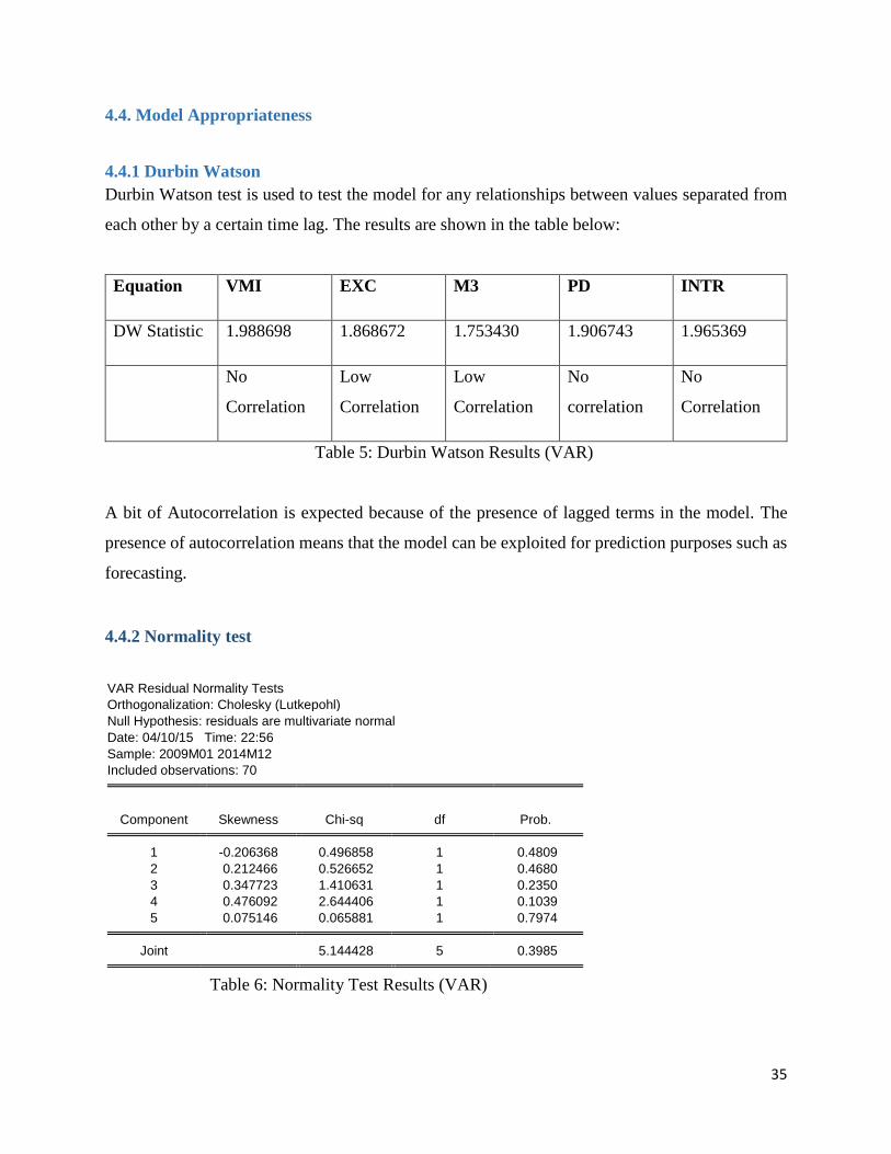
Durbin Watson test is used to test the model for any relationships between values separated from

each other by a certain time lag. The results are shown in the table below:

Equation VMI EXC M3 PD INTR

DW Statistic 1.988698 1.868672 1.753430 1.906743 1.965369

No

Correlation

Low

Correlation

Low

Correlation

No

correlation

No

Correlation

Table 5: Durbin Watson Results (VAR)

A bit of Autocorrelation is expected because of the presence of lagged terms in the model. The

presence of autocorrelation means that the model can be exploited for prediction purposes such as

forecasting.

4.4.2 Normality test

VAR Residual Normality Tests

Orthogonalization: Cholesky (Lutkepohl)

Null Hypothesis: residuals are multivariate normal

Date: 04/10/15 Time: 22:56

Sample: 2009M01 2014M12

Included observations: 70

Component Skewness Chi-sq df Prob. 1 -0.206368 0.496858 1 0.4809

2 0.212466 0.526652 1 0.4680

3 0.347723 1.410631 1 0.2350

4 0.476092 2.644406 1 0.1039

5 0.075146 0.065881 1 0.7974 Joint 5.144428 5 0.3985

Table 6: Normality Test Results (VAR)

36

For p < 0.05 we reject Null.

For p > 0.05 we fail to reject Null.

From the table above we can see that the residuals are normally distributed which is one of the

assumptions we made upon building the model.

4.5 Impulse Response Functions

The impulse response function measures the consequence of one unit increase in a particular

variable at time t holding all other innovations at all dates constant. Ordering used for analysis is

VMI, EXC, M3, PD and INTR. It is important in that the responses can change dramatically if the

ordering is changed.

4.5.1 Impulse response due to Funding and Debt Management (Strategy).

This strategy proposed in the ZIM-ASSET policy has the effect of increasing capital to

manufacturing industries as the Government will mobilize funding from domestic resources which

are said to be in abundance and readily available for exploitation and utilization. Government will

provide financial assistance to different sectors of the economy (manufacturing sector included).

This strategy will have an effect of increasing capital which in turn increases the chances of

manufacturing industries to get loans to recapitalize and improve capacity utilization. Hence we

shall observe how a unit increase in M3 will affect VMI and the other variables under study for a

period of 10 months (Jan to Oct 2015). The graph below shows results of a one standard deviation

shock to M3.

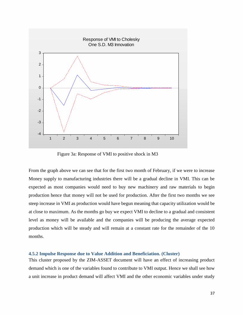
37

Figure 3a: Response of VMI to positive shock in M3

From the graph above we can see that for the first two month of February, if we were to increase

Money supply to manufacturing industries there will be a gradual decline in VMI. This can be

expected as most companies would need to buy new machinery and raw materials to begin

production hence that money will not be used for production. After the first two months we see

steep increase in VMI as production would have begun meaning that capacity utilization would be

at close to maximum. As the months go buy we expect VMI to decline to a gradual and consistent

level as money will be available and the companies will be producing the average expected

production which will be steady and will remain at a constant rate for the remainder of the 10

months.

4.5.2 Impulse Response due to Value Addition and Beneficiation. (Cluster)

This cluster proposed by the ZIM-ASSET document will have an effect of increasing product

demand which is one of the variables found to contribute to VMI output. Hence we shall see how

a unit increase in product demand will affect VMI and the other economic variables under study

-4

-3

-2

-1

0

1

2

3

1 2 3 4 5 6 7 8 9 10

Response of VMI to CholeskyOne S.D. M3 Innovation

38

for a period of 10 months (Jan to Oct 2015). The graph below shows results of a one standard

deviation shock to PD.

Figure 3b: Response of VMI to one positive shock in PD

If new markets are found and our products from our manufacturing companies are to be in demand,

we see a steep increase in VMI as we would have a destination for our goods and products will be

bringing in the needed capital to continue production. With time the production levels will have to

decline and reach a gradual consistent level as the markets would be saturated with the goods and

a normal demand would have been reached meaning a normal production level would have been

reached also.

Impulse responses of EXC, PD, and INTR to a unit shock to M3 and Impulse Reponses of EXC,

M3 and INTR to a unit shock to PD are shown in the index.

-2

-1

0

1

2

3

4

1 2 3 4 5 6 7 8 9 10

Response of VMI to CholeskyOne S.D. PD Innovation

39

4.6 Forecasting using developed VAR Model

Forecast for 2014 were done using Differenced data from 2009 and 2013 to check for the power

of the model for forecasting purposes and the following results were obtained :

For 95% confidence intervals, t (5, 0.025) = 2.571

Observation (2014) VMI (Actual 2014) VMIF (2014)

Jan -5.96 -0.21

Feb 11.4 6.78

Mar -7.38 -4.61

Apr 2.05 1.38-

May -.093 -0.58

June 6.78 5.23

July 0.186 0.02

Aug -3.20 -2.10

Sept 8.239 2.32

Oct -1.09 -0.03

Nov -6.30 -3.28

Dec 4.10 1.58

Table 7: VAR model forecast (2014)

40

4.7 VEC model Building

4.7.1 Johnsen Cointegration Test

The test if performed to check if the variables are cointegrated or not or if the variables have long

run association or not.

Null Hypothesis: None (there are no cointegrated variables, at most 1,2,3,4, and 5).

Series: VMI EXC M3 PD LC INTR Lags interval: 1 to 1

Likelihood 5 Percent 1 Percent Hypothesized Eigenvalue Ratio Critical Value Critical Value No. of CE(s)

0.507147 130.3098 94.15 103.18 None ** 0.403727 80.78168 68.52 76.07 At most 1 ** 0.235354 44.58770 47.21 54.46 At most 2 0.215253 25.80370 29.68 35.65 At most 3 0.095963 8.836150 15.41 20.04 At most 4 0.025027 1.774177 3.76 6.65 At most 5

L.R. test indicates at most 2 cointegrating equation(s) at 5% significance level

Table 8: Johansen Cointegration Results

From the results above we know that if any equations are found to be cointegrated we can run the

Vector Error Correction Model.

4.8 VEC Model Formulation

The presence of cointegration between variables indicates a long run relationship among the

variables under study hence the VEC model will be applied with the following variables found to

affect VMI in the earlier granger causality test at the lag length that was found to be appropriate

which is lag 1. The Resulting Model is shown on the next page.

41

Error Correction: D(VMI) D(EXC) D(M3) D(PD) D(INTR) CointEq1 -0.821441 0.008203 -1837.873 1.241718 -0.000355

(0.12244) (0.00690) (2081.78) (1.12544) (0.06067)

[-6.70908] [ 1.18831] [-0.88284] [ 1.10332] [-0.00585]

D(VMI(-1)) 0.095131 -0.012193 1907.020 -0.973121 0.125644

(0.10408) (0.00587) (1769.64) (0.95669) (0.05157)

[ 0.91402] [-2.07784] [ 1.07763] [-1.01717] [ 2.43639]

D(EXC(-1)) 5.443703 0.004810 6559.457 -29.77094 -0.785198

(2.26810) (0.12788) (38564.3) (20.8484) (1.12382)

[ 2.40011] [ 0.03761] [ 0.17009] [-1.42797] [-0.69869]

D(M3(-1)) -6.54E-06 9.01E-07 -0.273536 -3.48E-05 -1.84E-06

(9.0E-06) (5.1E-07) (0.15312) (8.3E-05) (4.5E-06)

[-0.72590] [ 1.77447] [-1.78641] [-0.41993] [-0.41278]

D(PD(-1)) 0.003614 0.000212 -280.2686 -0.335278 -0.001421

(0.01345) (0.00076) (228.759) (0.12367) (0.00667)

[ 0.26861] [ 0.27969] [-1.22517] [-2.71106] [-0.21314]

D(INTR(-1)) -1.123740 -0.007764 -2784.700 -2.531171 0.058807

(0.25900) (0.01460) (4403.75) (2.38073) (0.12833)

[-4.33876] [-0.53170] [-0.63235] [-1.06319] [ 0.45824]

C 0.410085 -0.041263 82526.40 7.584445 0.194371

(0.92869) (0.05236) (15790.5) (8.53655) (0.46016)

[ 0.44157] [-0.78806] [ 5.22634] [ 0.88847] [ 0.42240]

R-squared 0.678582 0.600651 0.978670 0.541361 0.729723

Adj. R-squared 0.638447 0.594999 0.911949 0.529586 0.646839

Sum sq. resids 2509.422 7.976787 7.25E+11 212027.7 616.0832

S.E. equation 6.311267 0.355831 107309.7 58.01309 3.127155

F-statistic 14.41590 1.175113 1.139076 1.728653 1.565123

Log likelihood -224.6016 -23.30711 -906.4813 -379.8849 -175.4467

Akaike AIC 6.617190 0.865917 26.09946 11.05385 5.212764

Schwarz SC 6.842039 1.090767 26.32431 11.27870 5.437613

Mean dependent -0.008571 0.013429 64906.67 3.737227 0.061143

S.D. dependent 9.289791 0.358530 107956.6 59.82275 3.203069 Determinant resid covariance (dof adj.) 1.34E+15

Determinant resid covariance 7.89E+14

Log likelihood -1697.199

Akaike information criterion 49.63425

Schwarz criterion 50.91911

Table 9: VEC Model

42

4.9 Model Appropriateness

4.9.1 Durbin Watson

Durbin Watson test is used to test the model for any relationships between values separated from

each other by a certain time lag. The results are shown in the table below:

Equation VMI EXC M3 PD INTR

DW Statistic 2.101741 1.901956 1.758153 1.93466 1.966

No

Correlation

No

Correlation

Low

Correlation

No

correlation

No

Correlation

Table 10: Durbin Watson Test Results (VEC)

4.9.2 Normality Test

Component Skewness Chi-sq df Prob. 1 0.346347 1.399486 1 0.2368

2 0.142195 0.235894 1 0.6272

3 0.372270 1.616821 1 0.2035

4 0.572660 3.825957 1 0.0505

5 0.127010 0.188200 1 0.6644 Joint 7.266358 5 0.2016

Table11:NormalityTestResults(VEC)

For p < 0.05 we reject Null.

For p > 0.05 we fail to reject Null.

From the table above we can see that the residuals are normally distributed which is one of the

assumptions we made upon building the model.

43

4.10 Impulse Response Functions Using VEC Model

Ordering used for analysis is VMI, EXC, M3, PD and INTR. It is important in that the responses

can change dramatically if the ordering is changed.

4.10.1 Impulse response due to Funding and Debt Management (Strategy).

This strategy proposed in the ZIM-ASSET policy has the effect of increasing capital to

manufacturing industries as the Government will mobilize funding from domestic resources which

are said to be in abundance and readily available for exploitation and utilization. Government will

provide financial assistance to different sectors of the economy (manufacturing sector included).

This strategy will have an effect of increasing capital which in turn increases the chances of

manufacturing industries to get loans to recapitalize and improve capacity utilization. Hence we

shall observe how a unit increase in M3 will affect VMI and the other variables under study for a

period of 10 months (Jan to Oct 2015). The graph below shows results of a one standard deviation

shock to M3.

Figure 4: Impulse Response of VMI due to a positive shock in M3 (VECM)

-1.6

-1.2

-0.8

-0.4

0.0

0.4

1 2 3 4 5 6 7 8 9 10

Response of VMI to CholeskyOne S.D. M3 Innovation

44

From the graph above we can see that for the first two month of February as is the VAR, if we

were to increase Money supply to manufacturing industries there will be a gradual decline in VMI.

This can be expected as most companies would need to buy new machinery and raw materials to

begin production hence that money will not be used for production. After the first two months we

see steep increase in VMI as production would have begun meaning that capacity utilisation would

be at close to maximum. As the months go buy we expect VMI to decline but unlike the results of

the VAR model the decline does not level off to a gradual and consistent level but it actually

becomes negative and remains so for the remainder of the months.

4.10.2 Impulse Response due to Value Addition and Beneficiation. (Cluster)

This cluster proposed by the ZIM-ASSET document will have an effect of increasing product

demand which is one of the variables found to contribute to VMI output. Hence we shall see how

a unit increase in product demand will affect VMI and the other economic variables under study

for a period of 10 months (Jan to Oct 2015). The graph below shows results of a one standard

deviation shock to PD.

45

Figure 5: Impulse Response of VMI due to a positive shock in PD (VECM)

If new markets are found and our products from our manufacturing companies are to be in demand,

we see a steep increase in VMI as we would have a destination for our goods and products will be

bringing in the needed capital to continue production. With time the production levels will have to

decline and reach a gradual consistent level but unlike the VAR model this consistent level does

not harbor around the center line but is clearly positive for the remainder of the 10 months.

Impulse responses of EXC, PD, and INTR to a unit shock to M3 and Impulse Reponses of EXC,

M3 and INTR to a unit shock to PD using the VEC model are shown in the index

-0.4

0.0

0.4

0.8

1.2

1.6

2.0

1 2 3 4 5 6 7 8 9 10

Response of VMI to CholeskyOne S.D. PD Innovation

46

4.11 Forecasting using developed VEC Model

Forecast for 2014 were done using data from 2009 and 2013 to check for the power of the model

for forecasting purposes and the following results were obtained:

For 95% confidence intervals, t(5, 0.025) = 2.571

Observation (2014) VMI (Actual 2014) VMIF (2014)

Jan 82.1 90.25

Feb 93.5 90.2

Mar 86.1 90.1

Apr 88.2 90.1

May 87.3 90.05

June 94.0 89.99

July 93.9 89.94

Aug 90.7 89.89

Sept 98.9 89.84

Oct 97.8 89.79

Nov 91.5 89.73

Dec 95.6 89.68

Table 12: VEC model Forecast (2014)

47

4.12 Comparison of Models in their Forecasting power

Period

(2009)

VAR Model Actual VAR Model

Forecast

Error % Error

Oct -1.09 -0.03 -1.06 97.24

Nov -6.30 -3.28 -3.02 47.93

Dec 4.10 1.58 2.52 61.46

Table 13a: % Error in forecasting power of VARM

Period

(2009)

VEC Model Actual VEC Model

Forecast

Error % Error

Oct 97.8 89.79 8.01 8.19

Nov 91.5 89.73 1.77 1.93

Dec 95.6 89.68 5.92 6.19

Table 13b: % Error in forecasting power of VECM

Period (2009) VAR Model % Error VEC Model % Error

Oct 97.24 8.19

Nov 47.93 1.93

Dec 61.46 6.19

Table13c: Comparison of error in forecasting power of VARM and VECM

4.13 Conclusion

From the results given in the table 14c, considering the forecasting error of the two models, it is

safe to conclude that the model with the least percentage errors in forecasting is the VEC model.

Forecast for VMI values for the coming years will be done using the model developed from

stationary data (VEC) model.

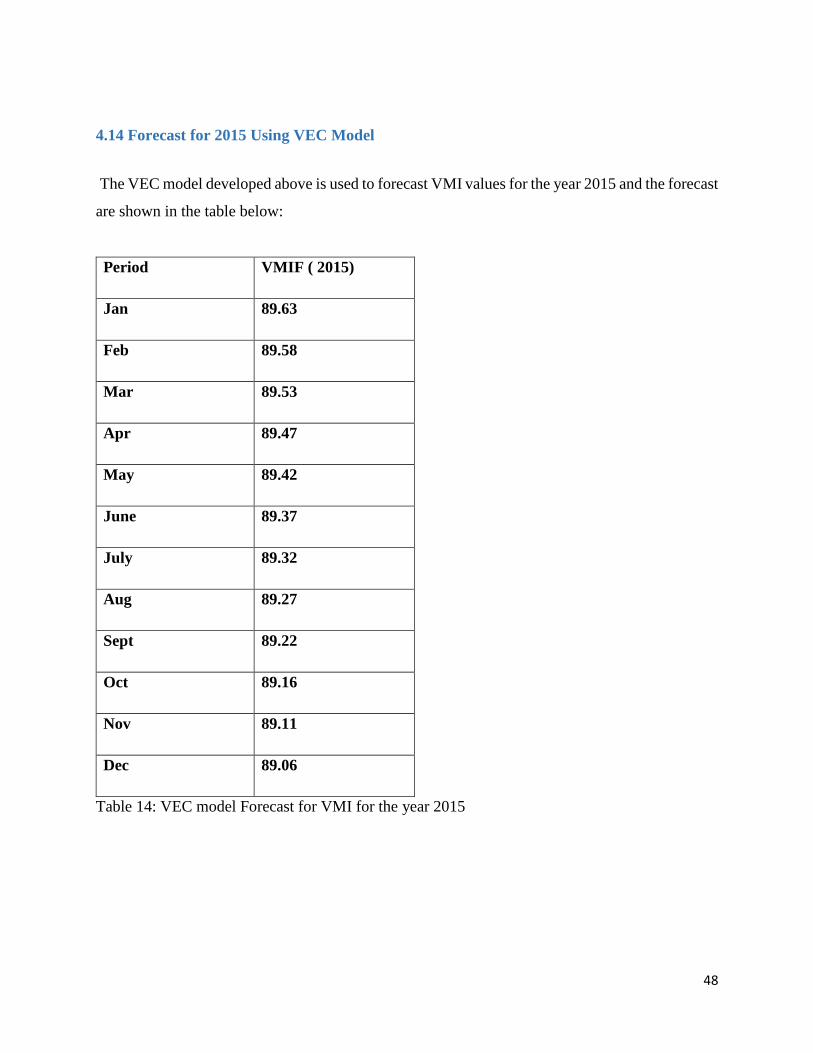
48

4.14 Forecast for 2015 Using VEC Model

The VEC model developed above is used to forecast VMI values for the year 2015 and the forecast

are shown in the table below:

Period VMIF ( 2015)

Jan 89.63

Feb 89.58

Mar 89.53

Apr 89.47

May 89.42

June 89.37

July 89.32

Aug 89.27

Sept 89.22

Oct 89.16

Nov 89.11

Dec 89.06

Table 14: VEC model Forecast for VMI for the year 2015

49

CHAPTER FIVE

5.1 Conclusion and Recommendations

The following chapter aims to give a brief summary of the results obtained and any

recommendations as to ways of improving the research better based on the results obtained. The

chapter also presents ideas on changes to policies that will enable the manufacturing sector to be

the echelon of all industries in Zimbabwe.

5.1.1 Conclusions drawn from the study

From my study it was determined that the variables were interrelated and cointegrated. It was seen

that exchange rate, money supply product demand and interest rate had an effect on the future

values of Volume of manufacturing index. And while using impulse response functions it was

determined that a unit shock in some of the variables mentioned above could either have a positive

or negative effect on the variables because the variables are interrelated.

From the study we were able to determine that the most influential constraint to VMI was Money

supply as increasing M3 saw a steep increase in the value of VMI within a short period of time.

Impulse response analysis was done for both the VAR and VEC models and we were able to trace

the effect on one standard deviation shock/ increase in money supply and product demand on the

future (10 Months) values of VMI. The overall effect was an increase in VMI.

Forecast for 2014 were carried out to check the power of the model in forecasting and it was found

that the VEC model produced better forecast. Using the VEC model VMI values for 2015 were

able to be forecasted leading me to conclude that there is indeed a significant difference in the

forecasting power of the VAR and VEC model and the VEC model being the better of the two.

All variable that are were proposed to affect VMI based on a theoretical view point were found to

indeed affect future values of VMI except for labor cost. This might be so because even if

employees are paid more money , which by the way will not be production based, they generally

50

produce the same output as before the increase in payment because unlike machines as humans we

tire much faster and have limited labor hours that we can take per day hence production would

generally remain the same

Policy changes are indeed explainable using the models developed hence the models can be used

for policy analysis. Unfortunately levels of VMI are expected to continue declining as evidenced

by the 2015 forecast. Policies such as ZIM-ASSET (2014-2018) and other policies such as the

Industrial Development Policy (2013-2015) should be fully and rightly implemented so that the

manufacturing sector and all other sectors in Zimbabwe can benefit.

5.2 Recommendations

Future researchers should attempt to use panel data and cover longer study duration of above10

years and consider adding other variables such as raw material availability. Other Dynamic and

more robust models such as GAS models could be used to analyze the econometric situation of

Zimbabwe in connection to the manufacturing industry. Lag selection is a major issue of concern

when dealing with VAR models hence a more appropriate lag selection criteria could be developed

that does not tend to over-fit the data hence losing degrees of freedom and making the model

unreliable for forecasting. Stationarity of the data also brings forth another problem because as

you try to make the data stationary you in turn lose valued data that could have contributed

considerably in model formulation hence it a model that can take both stationary and non-

stationary data can be developed it would be better.

51

References

Boedoloi, S.D. (2011). Interdependence of US industries sector using VAR.2011

Bukola, T.O. Support Vector Regression for non-stationary time series. University of Tennessee

Knoxville.

Confederation of Zimbabwean Industries In-house magazine. (January-April 2011).

Effects of changes in foreign exchange rates (IASC Foundation).

Errunza, V, Losq, E. (1985). International asset pricing under mild segmentation: Theory and

test. Journal of Finance 40, 105—124.

Fanelli, L. (2012). The specification of the Uni-Equatinal Dynamic econometric model.

University of Bologna

Giorgio, E and Primiceri. Time varying Structural Vector Auto-regressions and monetary policy.

North-western University. July 2004.

Gono, G. Press Statement on measures to improve liquidity (RBZ Governor) 2011

Granger, CWJ and Jin-Lung Lin, 1994,”Causality in the long run,” Econometric Theory, 11, 530-

536.

Guell, R.C. Econometrics today. 4th ed.

Gujaratim, N. (2004). Basic Econometrics.

Harvey, A.C., (1989). Forecasting, Structural Time Series Models.

Hon Professor Ncube, W. (MP). Zimbabwe’s Industrial Development Policy. (2011-2015).

http://Time series/ Why use Vector Error Correction Model/ Cross Validation.html

http://VAR (p) Models/Stata/2015,Simulink.htm

http://Var/Economic forecasting techniques and their applications/Business management book

chpt 2/ Global.hm

http://VAR: Stability analysis for VAR systems.

52

http://Vector Auto-regressive Models/Mat lab/Simulink.htm.

http://wikipidea.org/ wiki/ libour.html

http://www.imf.org/external/pubs/ft/weo/2009/update/01/index.htm.

http://www.wikipedia/Autoregressive Conditional heteroskedasticity.

Hyeongwo, K. Generalized Impulse Response Analysis: General or Extreme. Auburn University.

International Monetary Fund. January 2009. World Economic Outlook Update.

Jin_Lung, L. (2006). Teaching notes on the Impulse Response Function and Structural VAR.

Academia Sinica, Department. National Chegchi University 2006.

Kalman Filter. Cambridge: Cambridge Univ. Press.

Li, J (2006). Small business and entrepreneurship research in china, a special issue. Journal of

small Business and enterprise development, Vol.13 (2).

Luetkepohl, H. (2011). Vector Autoregressive Models. Florence Department of Economics,

European University Institute.

Maddala, G.S. Introduction to econometrics. 2nd ed.

Mhlanga, F. Manufacturing sector under threat. Zimbabwe Independent (December 2014)

Ministry of Industry and Commerce. Trade and Manufacturing sector strategic plans for statistics

(2011-2015)

Mugabe, R.G. (2013). Zimbabwe Agenda for Sustainable Socio- Economic Transformation (ZIM-

ASSET) “Towards an Empowered Society and Growing Economy. (October 2013- December

2018).

Muponda, G. (2013). Zimbabwe needs a stable political and economic environment. The Herald,

6 June 2013.

Ojo, A.S and Ololade, O.F (2014). An assessment of the Nigerian manufacturing sector in the era

of globalization. (2014)

53

Paulsen and Tjostheim. A Vector Error Correction Model (VECM). Approach in Explaining the

Relationship between Interest Rate and Inflation towards Exchange Rate Volatility in Malaysia.

(2012)

Saunders, R. (1996). Economic Structural Adjustment Programme (ESAP), Fables 11. Available

from South African Report Achieves, Vol 1, No 4. July 1996.

Sims, C.A. (1980). “Macroeconomics and Reality,” Econometrics, 48, 1-48.

Stock, J.H. and M.W. Watson (2001). “Vector Auto-regressions,” Journal of Economic

Perspectives, 15, 101-115.

Swanson, N. and C. W. J. Granger (1997), “Impulse response functions based on the causal

approach to residual Orthogonalization in Vector Auto-regressions,” Journal of the American

Statistical Association, 92, 357-367.

Wakeford, J. Productivity, Wages and Employment in South Africa’s Manufacturing Sector (1970-

2002). March 2004.

Wint-Alvin G. and Gordon V. Shirley. (1995). Enhancing the International Competitiveness of the

Jamaican Manufacturing Sector. Mona: Department of Management Studies, University of the

West Indies.

Xu, Y. Dynamic linkages between China and US equity markets under two recent financial Crises.

June 2010.

Young, R.M. and Klein, L.R. (2006). An introduction to econometric forecasting and forecasting

models. Journal of forecasting. Vol 11, Issue 3 [assessed Nov 2006].

54

Appendix

70635649423528211471

1.0

0.5

0.0

-0.5

-1.0

Index

D1

EX

C

TS-Plot for D1 EXC

55

70635649423528211471

300

200

100

0

-100

-200

Index

D1

PD

TS-Plot for D1 PD

70635649423528211471

75

50

25

0

-25

-50

Index

D1

LC

TS-Plot for D1 LC

56

70635649423528211471

600000

500000

400000

300000

200000

100000

0

-100000

-200000

-300000

Index

D1

M3

TS-Plot for D1 M3

70635649423528211471

10

5

0

-5

-10

-15

-20

Index

D1

INT

R

TS-Plot for D1 INTR

57

-4

-3

-2

-1

0

1

2

3

1 2 3 4 5 6 7 8 9 10

Response of VMI to M3

-.10

-.05

.00

.05

.10

.15

.20

1 2 3 4 5 6 7 8 9 10

Response of EXC to M3

-30

-20

-10

0

10

20

1 2 3 4 5 6 7 8 9 10

Response of PD to M3

-1.0

-0.5

0.0

0.5

1.0

1.5

1 2 3 4 5 6 7 8 9 10

Response of INTR to M3

Response to Cholesky One S.D. Innovations ± 2 S.E.

58

VECM

-2

-1

0

1

2

3

4

1 2 3 4 5 6 7 8 9 10

Response of VMI to PD

-.08

-.04

.00

.04

.08

.12

1 2 3 4 5 6 7 8 9 10

Response of EXC to PD

-40,000

-30,000

-20,000

-10,000

0

10,000

20,000

30,000

1 2 3 4 5 6 7 8 9 10

Response of M3 to PD

-2.0

-1.5

-1.0

-0.5

0.0

0.5

1.0

1 2 3 4 5 6 7 8 9 10

Response of INTR to PD

Response to Cholesky One S.D. Innovations ± 2 S.E.

59

-1.6

-1.2

-0.8

-0.4

0.0

0.4

1 2 3 4 5 6 7 8 9 10

Response of VMI to M3

.00

.02

.04

.06

.08

.10

1 2 3 4 5 6 7 8 9 10

Response of EXC to M3

-14.0

-13.6

-13.2

-12.8

-12.4

-12.0

-11.6

-11.2

-10.8

1 2 3 4 5 6 7 8 9 10

Response of PD to M3

.3

.4

.5

.6

.7

.8

1 2 3 4 5 6 7 8 9 10

Response of INTR to M3

Response to Cholesky One S.D. Innovations

60

-0.5

0.0

0.5

1.0

1.5

2.0

1 2 3 4 5 6 7 8 9 10

Response of VMI to PD

.00

.01

.02

.03

1 2 3 4 5 6 7 8 9 10

Response of EXC to PD

36

40

44

48

52

56

60

1 2 3 4 5 6 7 8 9 10

Response of PD to PD

-1.20

-1.15

-1.10

-1.05

-1.00

-0.95

1 2 3 4 5 6 7 8 9 10

Response of INTR to PD

Response to Cholesky One S.D. Innovations

61

Residuals for VARM

-20

-10

0

10

20

I II III IV I II III IV I II III IV I II III IV I II III IV I II III IV

2009 2010 2011 2012 2013 2014

VMI Residuals

-1.2

-0.8

-0.4

0.0

0.4

0.8

1.2

I II III IV I II III IV I II III IV I II III IV I II III IV I II III IV

2009 2010 2011 2012 2013 2014

EXC Residuals

-400,000

-200,000

0

200,000

400,000

600,000

I II III IV I II III IV I II III IV I II III IV I II III IV I II III IV

2009 2010 2011 2012 2013 2014

M3 Residuals

-200

-100

0

100

200

300

I II III IV I II III IV I II III IV I II III IV I II III IV I II III IV

2009 2010 2011 2012 2013 2014

PD Residuals

-15

-10

-5

0

5

10

15

I II III IV I II III IV I II III IV I II III IV I II III IV I II III IV

2009 2010 2011 2012 2013 2014

INTR Residuals