A. Torbjörn Johansson and Mathias H. Andersson

Ambient Underwater Noise Levels at Norra Midsjöbanken during Construction of the Nord Stream Pipeline

Cover photos: copyright of Mathias Andersson (upper left, lower right) and Nord Stream AG (upper right, lower left).

Detta verk är skyddat enligt lagen (1960:729) om upphovsrätt till litterära och konstnärliga verk. All form av kopiering, översättning eller bearbetning utan medgivande är förbjuden.

This work is protected under the Act on Copyright in Literary and Artistic Works (SFS 1960:729). Any form of reproduction, translation or modification without permission is prohibited.

Titel Ambient Underwater Noise Levels at Norra Midsjöbanken during Construction of the Nord Stream Pipeline

Title Ambient Underwater Noise Levels at Norra Midsjöbanken during Construction of the Nord Stream Pipeline

Rapportnr/Report no FOI-R--3469--SE

Månad/Month Sept

Utgivningsår/Year 2012

Antal sidor/Pages 65 p

ISSN 1650-1942

Kund/Customer Nord Stream AG and Naturvårdsverket (Swedish Environment Protection Agency)

FoT område

Projektnr/Project no E28239 and B21005

Godkänd av/Approved by Lena Lund

Ansvarig avdelning Defence and Security, Systems and Technology

FOI-R--3469--SE

3

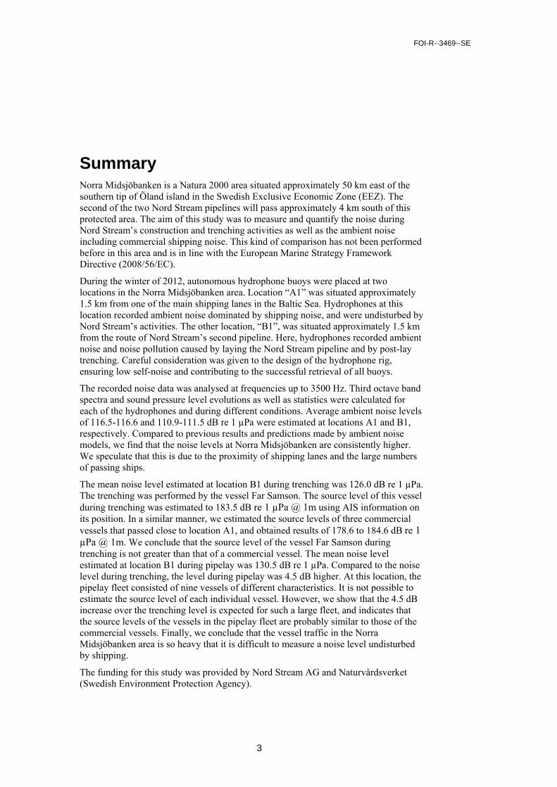
Summary Norra Midsjöbanken is a Natura 2000 area situated approximately 50 km east of the southern tip of Öland island in the Swedish Exclusive Economic Zone (EEZ). The second of the two Nord Stream pipelines will pass approximately 4 km south of this protected area. The aim of this study was to measure and quantify the noise during Nord Stream’s construction and trenching activities as well as the ambient noise including commercial shipping noise. This kind of comparison has not been performed before in this area and is in line with the European Marine Strategy Framework Directive (2008/56/EC).

During the winter of 2012, autonomous hydrophone buoys were placed at two locations in the Norra Midsjöbanken area. Location “A1” was situated approximately 1.5 km from one of the main shipping lanes in the Baltic Sea. Hydrophones at this location recorded ambient noise dominated by shipping noise, and were undisturbed by Nord Stream’s activities. The other location, “B1”, was situated approximately 1.5 km from the route of Nord Stream’s second pipeline. Here, hydrophones recorded ambient noise and noise pollution caused by laying the Nord Stream pipeline and by post-lay trenching. Careful consideration was given to the design of the hydrophone rig, ensuring low self-noise and contributing to the successful retrieval of all buoys.

The recorded noise data was analysed at frequencies up to 3500 Hz. Third octave band spectra and sound pressure level evolutions as well as statistics were calculated for each of the hydrophones and during different conditions. Average ambient noise levels of 116.5-116.6 and 110.9-111.5 dB re 1 µPa were estimated at locations A1 and B1, respectively. Compared to previous results and predictions made by ambient noise models, we find that the noise levels at Norra Midsjöbanken are consistently higher. We speculate that this is due to the proximity of shipping lanes and the large numbers of passing ships.

The mean noise level estimated at location B1 during trenching was 126.0 dB re 1 µPa. The trenching was performed by the vessel Far Samson. The source level of this vessel during trenching was estimated to 183.5 dB re 1 µPa @ 1m using AIS information on its position. In a similar manner, we estimated the source levels of three commercial vessels that passed close to location A1, and obtained results of 178.6 to 184.6 dB re 1 µPa @ 1m. We conclude that the source level of the vessel Far Samson during trenching is not greater than that of a commercial vessel. The mean noise level estimated at location B1 during pipelay was 130.5 dB re 1 µPa. Compared to the noise level during trenching, the level during pipelay was 4.5 dB higher. At this location, the pipelay fleet consisted of nine vessels of different characteristics. It is not possible to estimate the source level of each individual vessel. However, we show that the 4.5 dB increase over the trenching level is expected for such a large fleet, and indicates that the source levels of the vessels in the pipelay fleet are probably similar to those of the commercial vessels. Finally, we conclude that the vessel traffic in the Norra Midsjöbanken area is so heavy that it is difficult to measure a noise level undisturbed by shipping.

The funding for this study was provided by Nord Stream AG and Naturvårdsverket (Swedish Environment Protection Agency).

FOI-R--3469--SE

4

Sammanfattning Norra Midsjöbanken är ett Natura 2000-område beläget ca 50 km öster om Ölands Södra Udde i den svenska Exklusiva Ekonomiska Zonen (EEZ). Den andra av Nord Streams två pipelines kommer att passera ca 4 km söder om detta skyddade område. Målet med denna studie var att mäta och kvantifiera bullret under rörläggning och plogning av denna pipeline samt omgivningsbullret inklusive fartygsbuller. En dylik undersökning har inte förut utförts i detta område och ligger i linje med Havsmiljödirektivet (2008/56/EG).

Under vintern 2012 placerades autonoma hydrofonbojar på två platser i Norra Midsjöbanken-området. Bojen ”A1” placerades ca 1,5 km från en av de mest trafikerade fartygslederna i Östersjön. Den spelade in omgivningsbuller dominerat av fartygsbuller och förblev opåverkad av Nord Streams aktiviteter. Bojen ”B1” placerades ca 1,5 km från sträckningen av Nord Streams andra pipeline. Denna boj spelade in konstruktions- och plogningsbuller samt omgivningsbuller. Bojarnas placering och design valdes med stor omsorg, vilket bidrog till lågt egenbuller och lyckad bärgning av samtliga bojar.

Inspelade bullerdata analyserades vid frekvenser upp till 3500 Hz. Tredjedels oktavbandsspektra (tersbandsspektra) och ljudtrycksdata samt statistik av dessa beräknades. Medelvärdet av ljudtrycksnivån i bullret var 116,5 till 116,6 och 110,9 till 111,5 dB re 1 µPa vid A1 respektive B1. Vi jämför här med tidigare uppmätta bullernivåer i liknande miljöer och generella modeller för bullerspektra och finner att de här uppmätta nivåerna är konsistent högre än tidigare resultat. Vi spekulerar att detta beror på närheten till fartygsleder och det stora antalet passerande fartyg.

Vid position B1 uppskattades medel-bullernivån under plogning till 126,0 dB re 1 µPa. Plogningen utfördes av fartyget Far Samson. Källstyrkan för detta fartyg under plogning uppskattades med hjälp av AIS-information om dess position till 183,5 dB re 1 µPa @ 1m.På liknande sätt uppskattades källstyrkorna för tre handelsfartyg som passerade nära A1. Detta gav resultat från 178,6 till 184,6 dB re 1 µPa @ 1m. Vi drar slutsatsen att källstyrkan för Far Samson under plogning inte är högre än en källstyrka som kan uppmätas för ett handelsfartyg. Medel-bullernivån under rörläggning var 130,5 dB re 1 µPa. Detta är 4,5 dB högre än nivån under plogning. I Norra Midsjöbanken-området bestod rörläggningsflottan av nio fartyg. Det är inte möjligt att uppskatta källstyrkan hos varje fartyg i denna flotta. Dock visar vi att ökningen av bullernivån med 4,5 dB jämfört med plogningsnivån indikerar att källstyrkan för fartygen i rörläggningsflottan troligen är i nivå med de som beräknades för de tre handelsfartygen. Slutligen visar denna rapport att fartygstrafiken i området kring Norra Midsjöbanken är så intensiv att det är svårt att hitta ett avsnitt av inspelningarna som är ostört av fartygsbuller. Detta gör att vi inte kan uppskatta fartygstrafikens bidrag till omgivningsbullret.

Denna studie finansierades av Nord Stream AG och Naturvårdsverket.

FOI-R--3469--SE

5

Abbreviations

µPa microPascal

AIS Automatic Identification System

CPA Closest Point of Approach

DSG Autonomous hydrophone recording system manufactured by Loggerhead LLC, Sarasota, FL, USA.

Hz Hertz

NL Noise Level

nm Nautical mile (1,852 m)

RL Received Level

RMS Root-Mean-Square

PSD Power Spectral Density (unit: dB re 1 µPa2/Hz)

SL Source Level (unit: dB re 1 µPa @ 1 m)

SPL Sound Pressure Level (unit: dB re 1 µPa)

TL Transmission Loss

VMS Vessel Monitoring System

FOI-R--3469--SE

6

Table of Contents

Summary 3 

Sammanfattning 4 

Abbreviations 5 

Table of Contents 6 

1  Introduction 8 

1.1  Background ....................................................................................... 8 

1.2  Study area ......................................................................................... 9 

1.3  Shipping in the Baltic Sea ............................................................... 10 

1.4  Aim .................................................................................................. 11 

2  Preparations 12 

2.1  Selection of hydrophone rig locations ............................................. 12 

2.2  Hydrophone rig design .................................................................... 15 

2.3  DSG modifications and settings ...................................................... 16 

2.4  DSG calibration ............................................................................. 17 

2.5  Recording setup ............................................................................ 18 

2.5.1  Choice of sampling frequency ................................................ 18 2.5.2  Recording schedule ................................................................. 19 

2.6  Rig deployment and retrieval .......................................................... 20 

3  Environment 21 

3.1  Weather .......................................................................................... 21 

3.2  Acoustical environment ............................................................... 22 

4  Vessel passage statistics 23 

4.1  Survey period overview ............................................................... 23 

4.2  Pipelay ........................................................................................... 25 

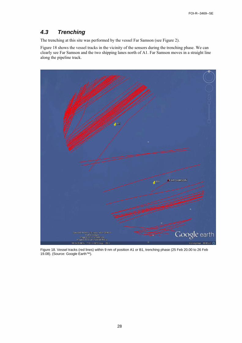
4.3  Trenching ....................................................................................... 28 

5  Noise spectra and levels 29 

5.1  Noise analysis methods .................................................................. 29 

5.2  Survey period overview .................................................................. 30 

5.3  Noise levels ................................................................................... 34 

5.3.1  Ambient noise ........................................................................... 34 5.3.2  Pipelay ....................................................................................... 37 

FOI-R--3469--SE

7

5.3.3  Trenching .................................................................................. 40 

6  Commercial vessel noise analysis 43 

6.1.1  Passage of “Subito” at A1, 28 Jan 12.02 ................................... 43 6.1.2  Passage of “Suono” at A1, 5 Mar 03.13 .................................... 43 6.1.3  Passage of “Finneagle” at B1, 5 Mar 13.27 ............................... 44 6.1.4  Source level estimation .............................................................. 45 

7  Ambient noise with no nearby vessels 47 

8  Discussion 49 

8.1  Ambient noise levels ................................................................... 49 

8.1.1  Comparison with Gerke, 2011 ................................................... 49 8.1.2  Comparison with ambient noise models .................................... 50 8.1.3  Other noise level reports ............................................................ 51 8.1.4  Summary of noise level comparisons ........................................ 51 

8.2  Noise levels during pipelay ............................................................ 52 

8.3  Noise levels during trenching ......................................................... 53 

8.4  Noise levels in the Norra Midsjöbanken Natura 2000 area ........... 56 

9  Conclusions 57 

10  Implications and suggested future work 58 

Acknowledgements 59 

References 60 

Appendix A. Acoustic terminology 62 

Appendix B. Nord Stream vessels and activity logs 63 

B.1  Activity logs .................................................................................. 63 

B.1.1  Pipelay ....................................................................................... 63 B.1.2  Boulder removal prior to post-lay trenching ......................... 63 B.1.3  Post-Lay Trenching.................................................................. 64 

B.2  Nord Stream Vessels ................................................................... 65 

FOI-R--3469--SE

8

1 Introduction

1.1 Background Anthropogenic noise from human activities has increased in our oceans and will increase even further in the near future due to increased shipping and ocean constructions. Shipping is the largest source of anthropogenic noise, although other industrial activities such as wind farms, seismic surveys and ocean construction add significant noise to the oceans (Ainslie et al., 2009; Hildebrand, 2009). The rise in shipping activities in the oceans have resulted in a 3-15 dB increase of ambient noise in the frequency interval 20-300 Hz in some deep water areas (Ross, 1993; Andrew et al., 2002). In a semi-detached sea like the Baltic Sea, it is very difficult to find a silent area without any shipping noise. The noise generated by a ship has a broadband character below 1000 Hz with a few narrowband peaks (tones). The machinery, the propeller and its shaft create most of the noise. Additionally, cavitation noise from the propeller and hydrodynamic flow around the hull adds to the projected acoustic signature of a ship (Arveson and Vendettis, 2000). The level of noise radiated by a ship is related to several factors such as its size, its machinery, speed, level of maintenance, mode of propulsion and operational characteristics.

The oceans are not in any way quiet even when anthropogenic acoustic noise is at a low level. Wind, waves, precipitation and biological activities such as snapping shrimps, grunting and croaking fish, and singing whales add natural ambient sound to the sea (Wenz, 1962; Hildebrand, 2009). Many marine animals rely on acoustics for their survival as they use sound for foraging, mating, communication and behavioural interactions. Animals that are exposed to anthropogenic noise can be adversely affected over a short time-scale or a long time-scale. Adverse effects can be subtle (e.g. temporary hearing loss, masking of important acoustic signals and behavioural effects) or obvious (e.g. worst case, death). Despite the intense usage of the oceans there are huge gaps in our understanding of the impact of noise on marine animals (Southall et al., 2007, OSPAR, 2009; Slabbekoorn et al., 2010). Lately, studies have been published on shipping noise where passive acoustic data are being combined with ship positions recorded by the Automatic Identification System (AIS). These allow for estimations on ships acoustical contribution to the ambient noise in remote areas and over long periods of time, see for example Hatch et al., 2008 and Merchant et al., 2012.

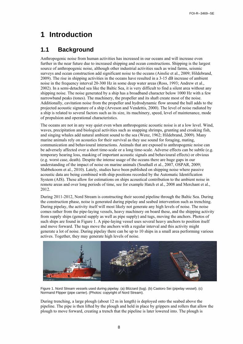
During 2011-2012, Nord Stream is constructing their second pipeline through the Baltic Sea. During the construction phase, noise is generated during pipelay and seabed intervention such as trenching. During pipelay, the activity itself will most likely not generate any high levels of noise. The noise comes rather from the pipe-laying vessels, heavy machinery on board these, and the shipping activity from supply ships (general supply as well as pipe supply) and tugs, moving the anchors. Photos of such ships are found in Figure 1. A pipe-laying vessel uses several heavy anchors to position itself and move forward. The tugs move the anchors with a regular interval and this activity might generate a lot of noise. During pipelay there can be up to 10 ships in a small area performing various actives. Together, they may generate high levels of noise.

Figure 1. Nord Stream vessels used during pipelay. (a) Blizzard (tug). (b) Castoro Sei (pipelay vessel). (c) Normand Flipper (pipe carrier). (Photos: copyright of Nord Stream).

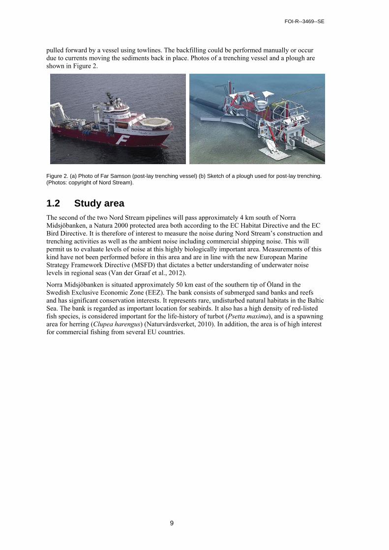
During trenching, a large plough (about 12 m in length) is deployed onto the seabed above the pipeline. The pipe is then lifted by the plough and held in place by grippers and rollers that allow the plough to move forward, creating a trench that the pipeline is later lowered into. The plough is

FOI-R--3469--SE

9

pulled forward by a vessel using towlines. The backfilling could be performed manually or occur due to currents moving the sediments back in place. Photos of a trenching vessel and a plough are shown in Figure 2.

Figure 2. (a) Photo of Far Samson (post-lay trenching vessel) (b) Sketch of a plough used for post-lay trenching. (Photos: copyright of Nord Stream).

1.2 Study area The second of the two Nord Stream pipelines will pass approximately 4 km south of Norra Midsjöbanken, a Natura 2000 protected area both according to the EC Habitat Directive and the EC Bird Directive. It is therefore of interest to measure the noise during Nord Stream’s construction and trenching activities as well as the ambient noise including commercial shipping noise. This will permit us to evaluate levels of noise at this highly biologically important area. Measurements of this kind have not been performed before in this area and are in line with the new European Marine Strategy Framework Directive (MSFD) that dictates a better understanding of underwater noise levels in regional seas (Van der Graaf et al., 2012).

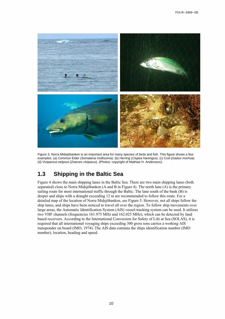
Norra Midsjöbanken is situated approximately 50 km east of the southern tip of Öland in the Swedish Exclusive Economic Zone (EEZ). The bank consists of submerged sand banks and reefs and has significant conservation interests. It represents rare, undisturbed natural habitats in the Baltic Sea. The bank is regarded as important location for seabirds. It also has a high density of red-listed fish species, is considered important for the life-history of turbot (Psetta maxima), and is a spawning area for herring (Clupea harengus) (Naturvårdsverket, 2010). In addition, the area is of high interest for commercial fishing from several EU countries.

FOI-R--3469--SE

10

Figure 3. Norra Midsjöbanken is an important area for many species of birds and fish. This figure shows a few examples. (a) Common Eider (Somateria mollissima). (b) Herring (Clupea harengus). (c) Cod (Gadus morhua). (d) Viviparous eelpout (Zoarces viviparus). (Photos: copyright of Mathias H. Andersson).

1.3 Shipping in the Baltic Sea Figure 4 shows the main shipping lanes in the Baltic Sea. There are two main shipping lanes (both separated) close to Norra Midsjöbanken (A and B in Figure 4). The north lane (A) is the primary sailing route for most international traffic through the Baltic. The lane south of the bank (B) is deeper and ships with a draught exceeding 12 m are recommended to follow this route. For a detailed map of the location of Norra Midsjöbanken, see Figure 5. However, not all ships follow the ship lanes, and ships have been noticed to travel all over the region. To follow ship movements over large areas, the Automatic Identification System (AIS) vessel-tracking system can be used. It utilizes two VHF channels (frequencies 161.975 MHz and 162.025 MHz), which can be detected by land based receivers. According to the International Conversion for Safety of Life at Sea (SOLAS), it is required that all international voyaging ships exceeding 300 gross tons carries a working AIS transponder on board (IMO, 1974). The AIS data contains the ships identification number (IMO number), location, heading and speed.

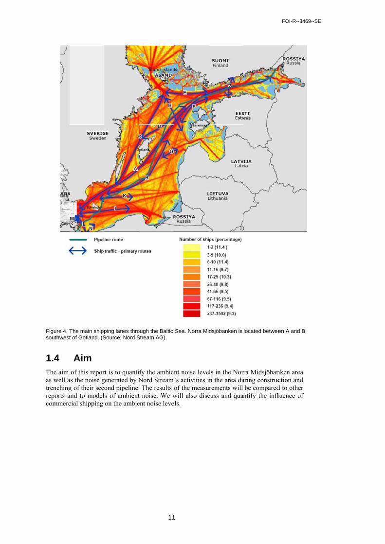
Figure 4. Tsouthwest

1.4 The aim as well atrenchingreports acommerc

The main shippt of Gotland. (S

Aim of this repor

as the noise gg of their secoand to modelcial shipping

ping lanes throSource: Nord S

rt is to quantigenerated by Nond pipeline.s of ambienton the ambie

11

ough the Baltic Stream AG).

fy the ambienNord Stream The results o

t noise. We went noise leve

1

Sea. Norra Mi

nt noise leve’s activities iof the measuwill also discels.

dsjöbanken is

ls in the Norrin the area duurements will cuss and quan

located betwee

ra Midsjöbanuring construc

be comparedntify the infl

FOI-R--3469--

en A and B

nken area ction and d to other luence of

-SE

FOI-R--3469--SE

12

2 Preparations

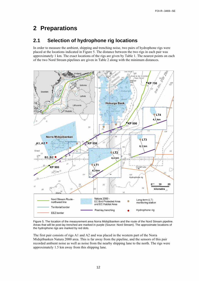
2.1 Selection of hydrophone rig locations In order to measure the ambient, shipping and trenching noise, two pairs of hydrophone rigs were placed at the locations indicated in Figure 5. The distance between the two rigs in each pair was approximately 1 km. The exact locations of the rigs are given by Table 1. The nearest points on each of the two Nord Stream pipelines are given in Table 2 along with the minimum distances.

Figure 5. The location of the measurement area Norra Midsjöbanken and the route of the Nord Stream pipeline. Areas that will be post-lay trenched are marked in purple (Source: Nord Stream). The approximate locations of the hydrophone rigs are marked by red dots.

The first pair consists of rigs A1 and A2 and was placed in the western part of the Norra Midsjöbanken Natura 2000 area. This is far away from the pipeline, and the sensors of this pair recorded ambient noise as well as noise from the nearby shipping lane to the north. The rigs were approximately 1.5 km away from this shipping lane.

Hydrophone rig

Hydrophone rig

B1,B2

A1,A2

FOI-R--3469--SE

13

The second pair, B1 and B2, was placed close to the Nord Stream pipeline and just south of the Norra Midsjöbanken Natura 2000 area. They recorded construction and trenching noise, but also ambient and shipping noise from the shipping lane to the south of the pipeline.

All rigs were deployed Jan 9 2012 and retrieved Apr 15 2012.

Table 1. The locations of the hydrophone rigs.

Rig ID Rig Location

Latitude Longitude Depth (m)

A1 56 09.954 N 17 08.184 E 28

A2 56 10.331 N 17 08.979 E 28

B1 55 59.802 N 17 20.464 E 40

B2 56 00.130 N 17 21.233 E 38

Table 2. The distances from the hydrophone rigs to the Nord Stream pipelines. The KP (kilometre points) values are Nord Stream’s designation of the location of the closest point on the respective pipeline.

Rig ID

Nearest Point on Pipeline 1 Location, Distance and KP

Nearest Point on Pipeline 2 Location, Distance and KP

Latitude Longitude Distance (m) KP Latitude Longitude Distance (m) KP

A1 55 58.862 N 17 20.463 E 24206 889.965 55 58.816 17 20.514 24306 889.555

A2 55 59.121 N 17 21.222 E 24372 889.040 55 59.075 17 21.272 24472 888.632

B1 55 59.116 N 17 21.209 E 1489 889.057 55 59.397 17 22.030 1593 888.057

B2 55 59.070 N 17 21.259 E 1589 888.648 55 59.351 17 22.080 1693 887.649

The selection of the rig locations were based on the following criteria:

The rigs should be as close to the respective pipeline / shipping lane as possible, obeying safety regulations and minimising the risk that a vessel passes straight overhead. This lead to the conclusion that a distance of 1.5 km to the source of interest was appropriate.

To be able to compare data i.e. reduce the acoustic variability between the rig locations, all rigs should be placed at similar depths and at locations with similar bottom characteristics and bathymetry.

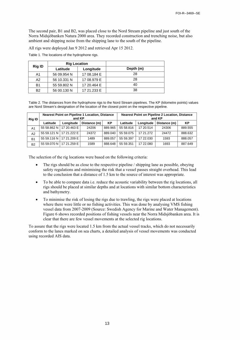
To minimise the risk of losing the rigs due to trawling, the rigs were placed at locations where there were little or no fishing activities. This was done by analysing VMS fishing vessel data from 2007-2009 (Source: Swedish Agency for Marine and Water Management). Figure 6 shows recorded positions of fishing vessels near the Norra Midsjöbanken area. It is clear that there are few vessel movements at the selected rig locations.

To assure that the rigs were located 1.5 km from the actual vessel tracks, which do not necessarily conform to the lanes marked on sea charts, a detailed analysis of vessel movements was conducted using recorded AIS data.

FOI-R--3469--SE

14

Figure 6. VMS recorded positions of EU ( “!”) and Swedish (“(“) fishing vessels moving at less than 5 knots near the Norra Midsjöbanken area, 2007-2009. Hydrophone rigs A1 and A2 are placed near the “H1B” marker, while rigs B1 and B2 are placed near the “H2B” marker. (Source: Swedish Agency for Marine and Water Management.)

!!

!

!

!

!

!

!

!

!

!

!

!

!!!

!!!!

!

!

!

!

!

!!

!

!!!!!!

!!!!!!!!!!!

!

!

!!

!!!!!!

!

!

!

!!

!

!

!

!

!!

!!!!!!!!!!

!

!!

!!

!

!

!

!

!

!!!!!

!!

!

!

!

!

!!!!!!!

!! !

!

!!!

!

!

!

!

!

!!!!!!!!

!

!

!

!

!

!!!!!!!!

!

!

!

!

! !

!

!

!

!!!!!

! !

!!

!

! !!

!

!!!

!!!!!!!

!

!

!!!! !!!

!!!!!!!

!

! ! !!!!!!!

!

!

!

!

!

! !!!!!

!!

!

!!!!!!!!

!

!!!!!!!!!

!

!

!

!!! ! !!!!!!

!!!

!

!

!!

!!

!

!

!!

!!!!!!!!!

!

!

!

!

!

!

!

!

!

!

!

!

!

!

!

!

!!

!

!

! !

!!

!

!

!

!

!

!

! !

!

!

!

! !!!

!

!

!

!

!!

!

!!

!

!!!

!

!

!

! !

!

!

!

!

!

!

!

!

!

!

!

!

!

!

!

! !!

! !!

!

!

!

!

!

!

!

!

!

!

!

!

!

!

!

!

!

!

!

!

!

!

!

!

!

!

!

!

!

!

!

!

! !

!

!

!

!

!

! !

!

!

!!

!

!!

!

!!

!

! !

!

!!

!

!

!

!

!

!

!

!

!

!!

!

!

!

!

!

!

!!

!

!

!

!

!

!

!

!

!

!

!!

!

!

!! !!

!!

!

!

!

!

!

!

!

!!

!

!

!!

! !!

!

!

!

!

!

!

!

!

!!

!

!

!

!

!

!

!

!

!

!! !

!

!!

!!!

!

!

!

!

!!

!!

!

!

!

!

!

!

!

!

!

!

!

!

!!!

!

!

!!

!

!

!

!

!

!

!!

!

!

!

!

!

!

!

!

!

!

!!

!

!

!

!

!

!

!

!

!

!

!

!

!!

!!

!

!

!

!

!

!

!!

!!

!

!

!

!

!

! !!

!

!

!

!

!

!

!

!

!

!

!

!

!

!

!!

!

!!

!

!

!

!!

! !

!

! !!

!

!!

!

!

!

!

!

!

!

!!

!

!!

!

!

!

!

!

!

!

!

!

!!

!!

!

!!

!

!!!

!

!!

!

!!

!

!

!!

!!

!

!

!

!!

!

!

!

!

!

!

!!!

!

!

!

!

!

!

!

!

!

!

! !

!

!

!

!

!!

!!!

!!!!!!!!!!!!!!

!

!

!!!!!!!!

!!

!

!

!!!!!!!!!!!!!

!

!

!

!

!

!

!!

!

!

!!!!!!!!!!!!

!

!

!

!!!!!!!!!!!!!

!

!

!

!!!!!!!!

!!

!!!!!!!!

!

!!

!

!!!!!!!

!!

!

!!!!!!

!

!

!!

!

!!!!! ! !! !

! !

!!!

!

!!!!!!!!!!!!

!

!

!!!!!!!

!!!

!!!!!!!

!

!!!!!!!!!

!

!!!!!!

!

!

!

!

!!!!!! !

!

!!!

!!!!!

!

!

! ! !

!!!!!

!

!!

!!!!!

!

!

!

!

!

!!!!!!!!!

!

!

!

!!!!!!!!!!!!!!!!!!!

!

!

!!!!!!!!

!

!

!

!

!!!!!!!!!!

!

!!

!!!!!

!

!

!!!!!!!!!!!!!

!

!!

!! !

!!

!!

! !!!!!!!!!

!

!

!!!!!!!!

!

!

!

!

!

!!!!!!!

!

!

!! !

!

!!!!!!! !

! !

!

!

!! ! !!!!!

!!!

!

!

!!

!

!

!

!

!

!!

!

!

!

!

!!

!

!!!!!!!!!

!

! !

!

!

!

!

!

!

!

!

!

!

!

!!!! !!!!!! !!

!!

!!!

!

!!

!

!

!

! !!

!

!

!

!

!

!

!

!

!

!

!

!

!

!! !

!

!!

!

!

!!

!!

!

!

!

!

!!

!

!

!!

!

!!!

!

!

!

!

! !!!!

!

!

!

!

!

!

!!

!

!

!!

!!!!!

!!

!

!

!!!

!

!

!

!

!

!

!

! !

!!

!

!

!

!

!!

!

!

!

!

!!

!

!

!

!!

!

!

!

!

!!

!

!

!

!

!

!

!

!

!

!

!

!

!!

!!

!

!

!

!

!

! !

!

!

!

!

!

!

!

!

!

!

!

!

!!

!

!

!

!

!

!

!

!

!

!

!

!

!

!

!

!

!

!

!

!

!

!

!!

!

!!

!

!!

!

!!

!!

! !

!

!

!

!

!!

!

!

! !

!

!!

!

!

!

!

!

!

!

!!

!

! !

!

!

!

!

!

!

!

!!

!

!

!!!! !

!!!!!!!!

!!

!

!

!

!

!

!

!

!! !

!

!

!

!!

!!

!

!

!

!

!

!

!

!

!

!

!

!

!

!

!

!

!

!

!

!

!

!

!

!

!

!

!

!

!

!

!

!

!

!

!

!

!

!

!

!

!

!

!!!

!

!

!!

!

!

!

! !!

!

!

!

!

!

!

!

!

!

!!

!

!

!

!

!

!

!!

!

!

!!!

!

!

!

!

!

!

!

!

!

!!

!

!

! !

!

!

!

!

!

!!

!!!

!

!

!

!

!

!

!

!

!

!

!

!

!

! !

!

!

!

!!

!

!

!

!

!

!

!

!

!

!

!

!

!

!

!

!

!!

!

!

!

!

!

!

!!

!

!

!

!

!!

!

!

!

!

!

!

!

!

!

!

!

!

!

!

!!

!

!

!

!

!

!

!

!

!

!

!

!

!

!

!!

!

!!

!!!

!

!

!

!

!!

!

!

!

!

!!

!

!

!!

!

!

!

!!

!!

!

!

!

!

!!

!

!

!

!

!

!

!

!!

!

!

!!

!

!

!!

!!

!

!

!

!

!

!!

!!

!

!

!

!

!

!

!

! !

!!

!

!

!! !

! !

!

!

!

!

!

! !

!

!!

!

!

!

!!

!

!

!

!

!

!

!

!

!

!

!

!!

!

!

!

!

!

!

!

!

!!

!

!

!

!

!

!

!

!

!

!!

!

!

!

!!

!

!!

!!

!

!

!

!

!

!

!

!

!

!

!

!

!!

!

!

!

!

!!! !

!

!

!

!!

!

!!

!! !

!!

!!

!

!

!

!!

!!!

!

!

!

!

!!

!

!!

!

!

!

!

!

!

!

!

!!

!

!

!

!

!

!

!

!

!

!

!!

!

!!

!

!

!

!

!!

!

!

!

!

!

!

!

!

!

!

!!

!

!!

!

!! !!

!

!!!

!!

!

!

!

!

!

!

!

!

!

!!

!

!

!

!! !

!!!

!

!

!

!!

!

!

!

!

!

!

!

!

!

!

!

!

!

!

!

!

!

!

!

!

!

!

!

!

!

!

!

!

!

!

!

!!

! !

!

!

!!

!

!!

!

!

!

!

!

!

!

!

!

!!!

!

!

!

!

!

!

!

!

!

!

!

!!

!

!

!

!!

!

! !

!

!

! !

!

!!!

!

!!!

!

!

!

!

!

!

! !

!!

!

!

!

!

!

!

!

!!

!

!!

!

!

!

!

!

!

!

!

!

!!

!

!!

!!!!

!!

!!

! ! !

!

!

!

!

!

!

!

!

!

!

!

!

!

!

!

!

!

!

!

!

!

!

!

! !

!

!!

!

!

!

!

!

!

!

!

!

!

!

!

!

!!

!

!

!

!

!!

!

!

!

!

! !

!

!

!

!

!

!

!

! !!!

!

!

!! !

!

!

!

!

!

!

!

!!

! !!!

!

!

!

!

!

! !

!

!

!

!

!

!!

!

!

!

!

! !

!

!

!

!

!

!

!

!

!

!

!

!

!

!

!!!

!!

!

!

!

!

!! !

!

!!!

!

!

!

!!

!

!

!

!

! !

!

!!

!

!

!

!

!

!

!!

!

!

!

!

!!!

!

!

!

!

!

!

!

!

! !!

!

!

!

!

!!

!

!

!

!

!!

!

!

!!

!

!

!

!!

!

!

!

!!!

!

! !

! !

!! !

!

!! !!

!

!!

!!!

!(

!(

!(

!(

!(

!(

!(

!(

!(!(!( !( !(!(!(!(!(!(!(!(!(

!(!( !(

!(!(!(

!(

!(

!(

!(!(!(

!(

!(

!(

!(

!(!(

!(

!(

!(

!(

!(

!(

!(

!(

!

!(

!(

!(

!(

!(

!( !(

!(

!(!(

!(

!(!(

!(

!(

!(!(

!(

!(

!( !(

!(

!(!(

!(

!(

!(

!(

!(

!(

!(!(

!(!(

!(

!( !(

!( !(

!(

!(

!(

!( !( !(!(!(

!(!(

!(

!(

!( !( !(

!(

!(

!(

!(!(!(

!(!(

!(

!(!(!(!(!(

!( !(

!(!(

!(

!(!(

!(

!(

!(

!(!(

!(!(

!( !(

!(

!(

!(!(

!(

!(

!(

!( !(

!(

!(

!(

!(!(

!(

!(

!(

!(!(

!(

!(

!(

!( !(

!(

!(!(

!(!(

!(!(!(!(!(!(!(!(!(!(!(!(!(!(!( !(

!(!( !(

!(

!(

!(!(

!(!(!(!(!(!(!(!(

!(!(

!(

!(

!(

!(

!(

!( !(!(!(

!(!(

!(!(

!(!(!(!(!(!(!(!(

!(!(

!(

!(

!(

!(

!(

!(

!(

!(

!(!(

!(!(

!(

!(

!(!(

!(

!(!(!(

!(

!(

!(

!(

!(

!(

!(

!(

!(

!(

!(!(

!(

!(

!(

!(

!(

!(

!(

!(

!(

!(!(

!(

!(

!(

!(

!(

!(

!(

!(

!(!( !( !(

!(!(

!(

!(

!(

!(!(

!(

!(

!(

GF

GF

GF

GF

17°50'0"E

17°40'0"E

17°40'0"E

17°30'0"E

17°30'0"E

17°20'0"E

17°20'0"E

17°10'0"E

17°10'0"E

17°0'0"E

56°25'0"N

56°25'0"N

56°20'0"N

56°20'0"N

56°15'0"N

56°15'0"N

56°10'0"N

56°10'0"N

56°5'0"N

56°5'0"N

56°0'0"N

56°0'0"N

55°55'0"N

55°55'0"N

FOI-R--3469--SE

15

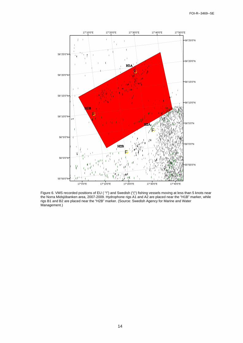
2.2 Hydrophone rig design The design of each of the four hydrophone rigs is shown schematically in Figure 7. When deployed, the rig extended approximately 2.5 m above the seabed.

Figure 7. Sketch of a hydrophone rig.

The rigs were anchored to a 60 kg reinforced concrete ballast weight. FOI has significant experience of using this type of rig for long-term offshore deployments in the Baltic Sea and has previously used ballasts of 20-30 kg. To further reduce of the risk of relocation by current, the ballast was increased to 60 kg.

Each rig was fitted with a DSG-Ocean autonomous hydrophone system (Loggerhead Instruments, Inc., Sarasota, FL, USA). The DSG-Ocean was equipped with a HTI-90-U hydrophone (High Tech, Inc., Gulfport, MS, USA). The frequency range of the hydrophone was 2 Hz to 20 kHz and it was rated to 100 m water depth. Its sensitivity was -186 dB re 1 V/µPa.

The DSG-Ocean (Figure 8) is an autonomous underwater recording platform which is capable of long-term deployment as well as scheduled recording. It is completely self-sustained and a set of standard alkaline batteries can power it for up to several months. FOI has used the DSG-Ocean in several projects and has found it to be reliable.

Water

Seafloor

Ballast weight (60 kg)

Acoustic releaser

Autonomous hydrophone

Buoy

2.5 m

Rope

FOI-R--3469--SE

16

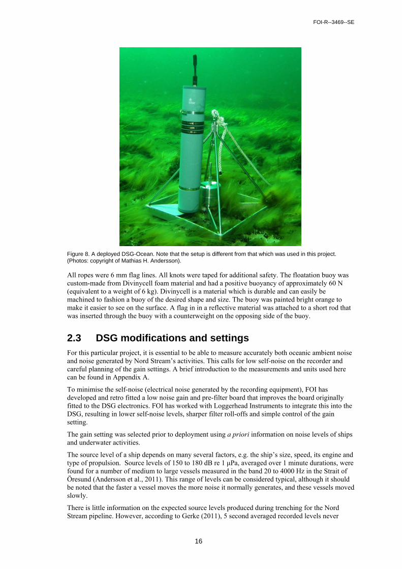
Figure 8. A deployed DSG-Ocean. Note that the setup is different from that which was used in this project. (Photos: copyright of Mathias H. Andersson).

All ropes were 6 mm flag lines. All knots were taped for additional safety. The floatation buoy was custom-made from Divinycell foam material and had a positive buoyancy of approximately 60 N (equivalent to a weight of 6 kg). Divinycell is a material which is durable and can easily be machined to fashion a buoy of the desired shape and size. The buoy was painted bright orange to make it easier to see on the surface. A flag in in a reflective material was attached to a short rod that was inserted through the buoy with a counterweight on the opposing side of the buoy.

2.3 DSG modifications and settings For this particular project, it is essential to be able to measure accurately both oceanic ambient noise and noise generated by Nord Stream’s activities. This calls for low self-noise on the recorder and careful planning of the gain settings. A brief introduction to the measurements and units used here can be found in Appendix A.

To minimise the self-noise (electrical noise generated by the recording equipment), FOI has developed and retro fitted a low noise gain and pre-filter board that improves the board originally fitted to the DSG electronics. FOI has worked with Loggerhead Instruments to integrate this into the DSG, resulting in lower self-noise levels, sharper filter roll-offs and simple control of the gain setting.

The gain setting was selected prior to deployment using a priori information on noise levels of ships and underwater activities.

The source level of a ship depends on many several factors, e.g. the ship’s size, speed, its engine and type of propulsion. Source levels of 150 to 180 dB re 1 μPa, averaged over 1 minute durations, were found for a number of medium to large vessels measured in the band 20 to 4000 Hz in the Strait of Öresund (Andersson et al., 2011). This range of levels can be considered typical, although it should be noted that the faster a vessel moves the more noise it normally generates, and these vessels moved slowly.

There is little information on the expected source levels produced during trenching for the Nord Stream pipeline. However, according to Gerke (2011), 5 second averaged recorded levels never

FOI-R--3469--SE

17

exceeded 150 dB re 1 μPa during measurements of Nord Stream construction noise at six different locations in German economic zone. These measurements were obtained at more than 1 km distance from the pipeline, but the exact distances are not clearly stated. This makes it difficult to estimate the source levels.

Source levels have been estimated during trenching for cables to an offshore wind farm. During construction of the North Hoyle offshore wind farm, it was found that cable trenching gave a source level of 178 dB re 1 μPa @ 1m, assuming a transmission loss of 22log10(range).

Based on the available data, we concluded that trenching will produce a source level that is equal to or less than that of a medium or large ship. However, a fleet of several vessels is involved in laying the Nord Stream pipeline. This fleet typically radiates more noise than a single vessel.

The expected frequency range covers frequencies up to 3500 Hz (see Section 2.5.1) which corresponds reasonably well with the range used by Andersson et al., 2011. Adding some margin to the expected source levels of shipping and Nord Stream’s activities, it was desired that the recording equipment should be able to measure noise corresponding to a level of up to at least 200 dB re 1 Pa @ 1m.

The rigs were located about 1 km from the vessel lane and the planned route of the second pipeline, respectively. Assuming a transmission loss of 17log10(range) which is typical of the Baltic Sea during winter, we will see at least 50 dB of transmission loss. Thus, the sensors should be able to measure sound levels of at least 150 dB re 1 Pa.

The DSG is a 16 bit recording system. Given a gain setting, the bit resolution gives a lower limit to the lowest signal level that can be accurately characterised. This is also influenced by the self-noise, e.g. electrical and quantisation noise, of the recording system.

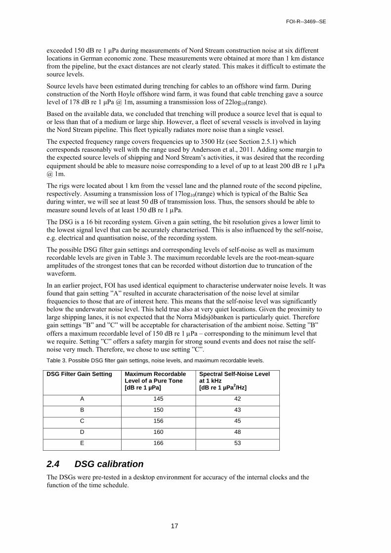
The possible DSG filter gain settings and corresponding levels of self-noise as well as maximum recordable levels are given in Table 3. The maximum recordable levels are the root-mean-square amplitudes of the strongest tones that can be recorded without distortion due to truncation of the waveform.

In an earlier project, FOI has used identical equipment to characterise underwater noise levels. It was found that gain setting ”A” resulted in accurate characterisation of the noise level at similar frequencies to those that are of interest here. This means that the self-noise level was significantly below the underwater noise level. This held true also at very quiet locations. Given the proximity to large shipping lanes, it is not expected that the Norra Midsjöbanken is particularly quiet. Therefore gain settings ”B” and ”C” will be acceptable for characterisation of the ambient noise. Setting ”B” offers a maximum recordable level of 150 dB re 1 Pa – corresponding to the minimum level that we require. Setting ”C” offers a safety margin for strong sound events and does not raise the self-noise very much. Therefore, we chose to use setting ”C”.

Table 3. Possible DSG filter gain settings, noise levels, and maximum recordable levels.

DSG Filter Gain Setting Maximum Recordable Level of a Pure Tone [dB re 1 µPa]

Spectral Self-Noise Levelat 1 kHz [dB re 1 µPa2/Hz]

A 145 42

B 150 43

C 156 45

D 160 48

E 166 53

2.4 DSG calibration The DSGs were pre-tested in a desktop environment for accuracy of the internal clocks and the function of the time schedule.

FOI-R--3469--SE

18

The complete rigs were assembled and brought to FOI’s field test site at Djupviken, near Berga south of Stockholm where they were placed in a marine environment that is similar to that at Norra Midsjöbanken. We verified that the acoustic releases were functioning properly and that the DSGs were watertight. The recording were performed according to a predetermined schedule and after recovery checked to verify that the schedule was correctly executed.

Finally, a detailed calibration of the DSGs was performed at FOI’s tank laboratory facility. Each DSG was placed in a specialised container and subjected to a carefully controlled sinusoidal signal. Pure tones at four different frequencies below 1 kHz were used. The DSG recorded signals were analysed to establish the response function. The response function of each DSG displayed less than ±0.2 dB variation with frequency. Therefore, we use a constant system sensitivity for each DSG. Table 4 shows the system sensitivities as well as the sensitivities of the hydrophones.

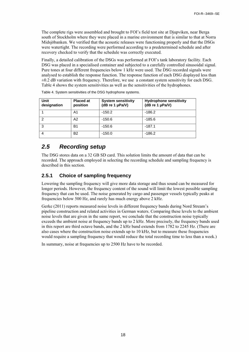
Table 4. System sensitivities of the DSG hydrophone systems.

Unit designation

Placed at position

System sensitivity (dB re 1 µPa/V)

Hydrophone sensitivity (dB re 1 µPa/V)

1 A1 -150.2 -186.2

2 A2 -150.6 -185.6

3 B1 -150.6 -187.1

4 B2 -150.0 -186.2

2.5 Recording setup The DSG stores data on a 32 GB SD card. This solution limits the amount of data that can be recorded. The approach employed in selecting the recording schedule and sampling frequency is described in this section.

2.5.1 Choice of sampling frequency

Lowering the sampling frequency will give more data storage and thus sound can be measured for longer periods. However, the frequency content of the sound will limit the lowest possible sampling frequency that can be used. The noise generated by cargo and passenger vessels typically peaks at frequencies below 500 Hz, and rarely has much energy above 2 kHz.

Gerke (2011) reports measured noise levels in different frequency bands during Nord Stream’s pipeline construction and related activities in German waters. Comparing these levels to the ambient noise levels that are given in the same report, we conclude that the construction noise typically exceeds the ambient noise at frequency bands up to 2 kHz. More precisely, the frequency bands used in this report are third octave bands, and the 2 kHz band extends from 1782 to 2245 Hz. (There are also cases where the construction noise extends up to 10 kHz, but to measure these frequencies would require a sampling frequency that would reduce the total recording time to less than a week.)

In summary, noise at frequencies up to 2500 Hz have to be recorded.

(

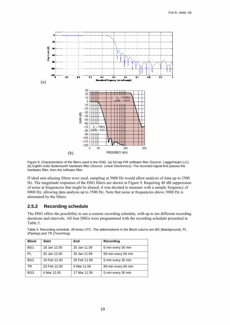
Figure 9. C(b) Eighthhardware

If ideal aHz. The mof noise a8000 Hz,attenuate

2.5.2

The DSGdurationsTable 5.

Table 5. R(Pipelay) a

Block

BG1

PL

BG2

TR

BG3

(a)

Characteristics order Butterwfilter, then the

anti-aliasing fmagnitude reat frequencie, allowing da

ed by the filte

Recordin

G offers the ps and interval

Recording scheand TR (Trenc

Start

18 Jan 12.00

25 Jan 12.00

18 Feb 12.00

25 Feb 12.00

6 Mar 12.00

(b)

s of the filters uorth hardware software filter.

filters were usesponses of thes that might bata analysis upers.

ng schedu

ossibility to uls. All four D

edule. All timesching).

End

25 Jan

29 Jan

0 25 Feb

0 6 Mar 1

17 Mar

19

used in the DSGfilter (Source:

sed, samplinghe DSG filterbe aliased, it p to 3500 Hz.

ule

use a custom SGs were pro

s UTC. The abb

R

11.59 5

11.59 5

b 11.59 5

11.59 5

r 11.59 5

9

G. (a) 63-tap FLinear Electron

g at 5000 Hz rs are shown iwas decided . Note that no

recording schogrammed w

breviations in t

Recording

5 min every 30

59 min every 6

5 min every 30

59 min every 6

5 min every 30

FIR software filtnics). The reco

would allow in Figure 9. Rto measure w

oise at freque

hedule, with with the record

he Block colum

0 min

60 min

0 min

60 min

0 min

ter (Source: Loorded signal firs

analysis of dRequiring 40 dwith a sample ncies above 3

up to ten diffding schedule

mn are BG (Bac

FOI-R--3469--

oggerhead LLCst passes the

data up to 250dB suppressi

e frequency of3000 Hz is

ferent recordie presented in

ckground), PL

-SE

C).

00 on f

ing n

FOI-R--3469--SE

20

During recording blocks PL (Pipelay) and TR (Trenching), the DSGs were set for nearly continuous recording. The recorded time span was selected to maximise the likelihood that pipelay and trenching would be captured in as much detail as possible.

For the characterisation of the ambient noise, it was sufficient to make short recordings at regular intervals. This schedule extends the time span in which recordings are made, thus capturing more of the natural noise variations, e.g. those that depend on weather. Table 5 shows that the DSGs were set to record ambient noise (BG) during three intervals.

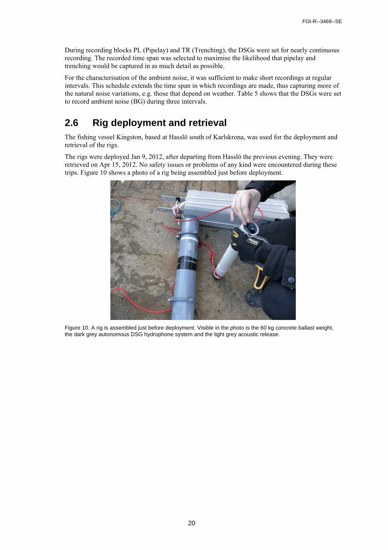
2.6 Rig deployment and retrieval The fishing vessel Kingston, based at Hasslö south of Karlskrona, was used for the deployment and retrieval of the rigs.

The rigs were deployed Jan 9, 2012, after departing from Hasslö the previous evening. They were retrieved on Apr 15, 2012. No safety issues or problems of any kind were encountered during these trips. Figure 10 shows a photo of a rig being assembled just before deployment.

Figure 10. A rig is assembled just before deployment. Visible in the photo is the 60 kg concrete ballast weight, the dark grey autonomous DSG hydrophone system and the light grey acoustic release.

FOI-R--3469--SE

21

3 Environment

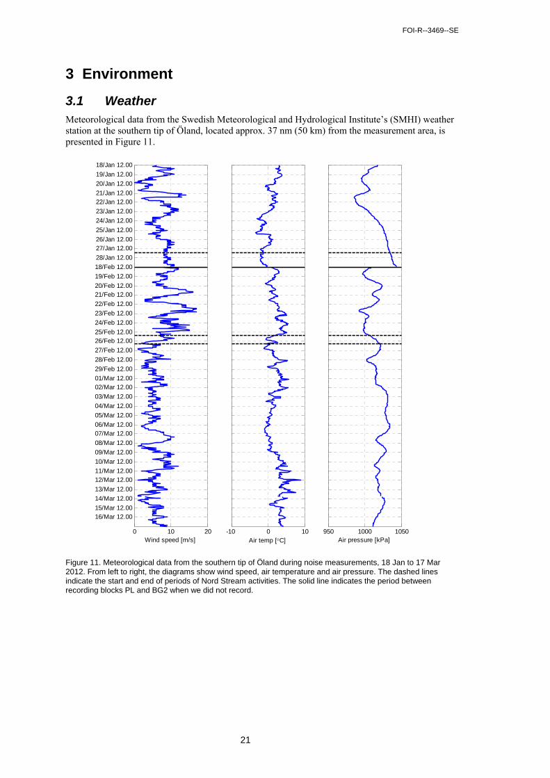
3.1 Weather Meteorological data from the Swedish Meteorological and Hydrological Institute’s (SMHI) weather station at the southern tip of Öland, located approx. 37 nm (50 km) from the measurement area, is presented in Figure 11.

Figure 11. Meteorological data from the southern tip of Öland during noise measurements, 18 Jan to 17 Mar 2012. From left to right, the diagrams show wind speed, air temperature and air pressure. The dashed lines indicate the start and end of periods of Nord Stream activities. The solid line indicates the period between recording blocks PL and BG2 when we did not record.

0 10 20

18/Jan 12.00

19/Jan 12.00

20/Jan 12.00

21/Jan 12.0022/Jan 12.00

23/Jan 12.00

24/Jan 12.00

25/Jan 12.00

26/Jan 12.0027/Jan 12.00

28/Jan 12.00

18/Feb 12.00

19/Feb 12.00

20/Feb 12.0021/Feb 12.00

22/Feb 12.00

23/Feb 12.00

24/Feb 12.00

25/Feb 12.0026/Feb 12.00

27/Feb 12.00

28/Feb 12.00

29/Feb 12.00

01/Mar 12.0002/Mar 12.00

03/Mar 12.00

04/Mar 12.00

05/Mar 12.00

06/Mar 12.0007/Mar 12.00

08/Mar 12.00

09/Mar 12.00

10/Mar 12.00

11/Mar 12.0012/Mar 12.00

13/Mar 12.00

14/Mar 12.00

15/Mar 12.0016/Mar 12.00

Wind speed [m/s]-10 0 10

Air temp [C]950 1000 1050

Air pressure [kPa]

FOI-R--3469--SE

22

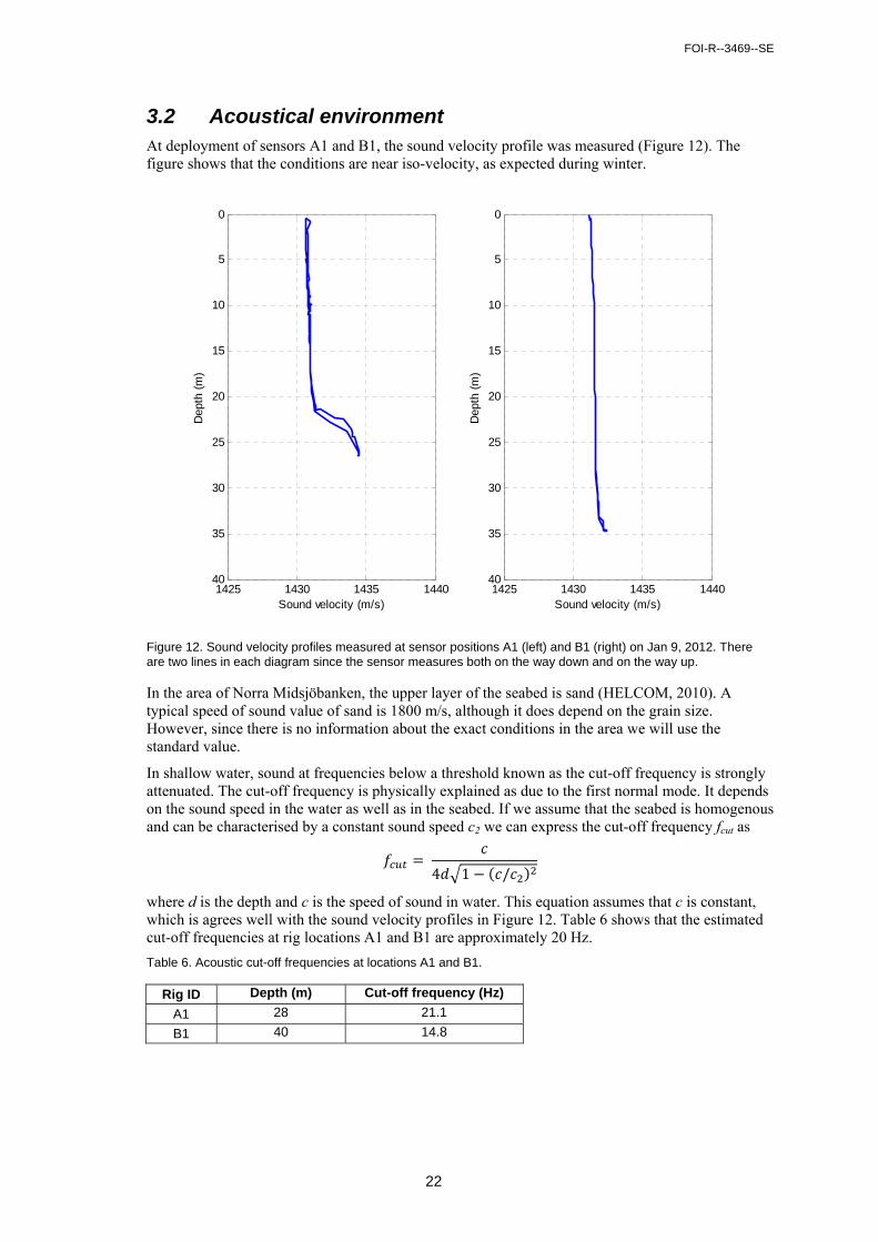
3.2 Acoustical environment At deployment of sensors A1 and B1, the sound velocity profile was measured (Figure 12). The figure shows that the conditions are near iso-velocity, as expected during winter.

Figure 12. Sound velocity profiles measured at sensor positions A1 (left) and B1 (right) on Jan 9, 2012. There are two lines in each diagram since the sensor measures both on the way down and on the way up.

In the area of Norra Midsjöbanken, the upper layer of the seabed is sand (HELCOM, 2010). A typical speed of sound value of sand is 1800 m/s, although it does depend on the grain size. However, since there is no information about the exact conditions in the area we will use the standard value.

In shallow water, sound at frequencies below a threshold known as the cut-off frequency is strongly attenuated. The cut-off frequency is physically explained as due to the first normal mode. It depends on the sound speed in the water as well as in the seabed. If we assume that the seabed is homogenous and can be characterised by a constant sound speed c2 we can express the cut-off frequency fcut as

4 1 /

where d is the depth and c is the speed of sound in water. This equation assumes that c is constant, which is agrees well with the sound velocity profiles in Figure 12. Table 6 shows that the estimated cut-off frequencies at rig locations A1 and B1 are approximately 20 Hz.

Table 6. Acoustic cut-off frequencies at locations A1 and B1.

Rig ID Depth (m) Cut-off frequency (Hz)

A1 28 21.1

B1 40 14.8

1425 1430 1435 1440

0

5

10

15

20

25

30

35

40

Sound velocity (m/s)

Dep

th (

m)

1425 1430 1435 1440

0

5

10

15

20

25

30

35

40

Sound velocity (m/s)

Dep

th (

m)

FOI-R--3469--SE

23

4 Vessel passage statistics Here we present both overview statistics and details of vessel movements during the construction and trenching phases. AIS data were recorded from Jan 18 to Mar 17, 2012, and was provided by the Swedish Maritime Administration (SMA).

We identified the vessels that passed within 9 nautical miles (16 658 m) of each of the sensor rigs A1 and B1. For each of those vessels, the closest point of approach (CPA) was determined as well as the range at CPA. Once a vessel was found to be inside the 9 nm range limit, its CPA was determined and its signal was then blocked for 4 hours in order to avoid multiple detections of the same vessel. This ensures that a passing vessel is only counted once. Nord Stream’s vessels that remain in the area of B1 were however counted multiple times, but since they are so few this has only a minor effect on the results.

VMS data of fishing vessels was not used here because its poor temporal resolution of 1 data point per hour implies that rapidly moving fishing vessels may pass through the 9 nm area without being logged. Further, the VMS statistics in Section 2.1 show that fishing activities were low at the rig locations.

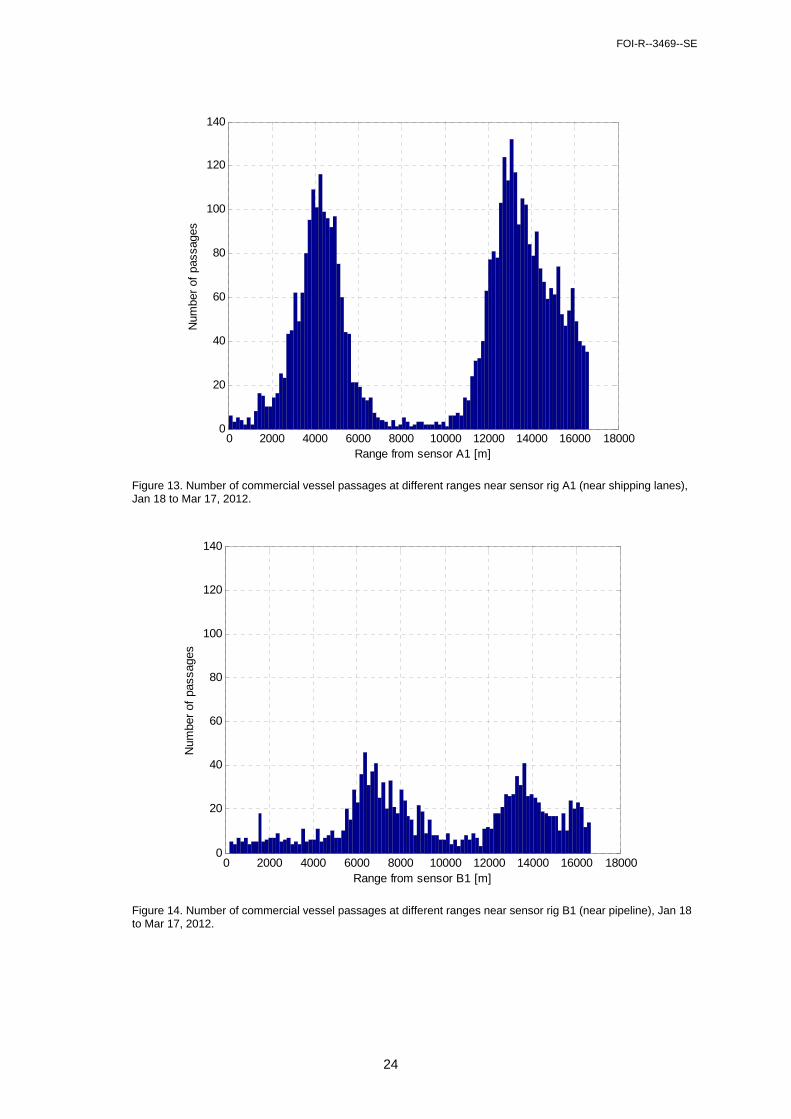
4.1 Survey period overview Here, we present statistics of passing vessels and their CPA ranges in Figure 13 (rig A1) and Figure 14 (rig B1).

There are shipping lanes within 9 nm of both A1 and B1, but the lane close to A1 is both closer to the respective rig position and sees more traffic. This can clearly be seen by comparing the figures. There are many more vessel passages near position A1 than near B1, and there are also a relatively large number of passages below a range of 6000 m as compared to the results near B1. The shipping lane north of A1 is divided into two one-way lanes, which results in the two peaks in the histogram for the A1 data. Most vessels stay in the shipping lanes, but not all. A total of 1390 vessels passed within 5 km of A1 during the entire measurement period of Jan 18 to Mar 17, 2012. By dividing this number by the 60 day duration of the measurement period, an average daily number of passages within 5 km of 23 is found.

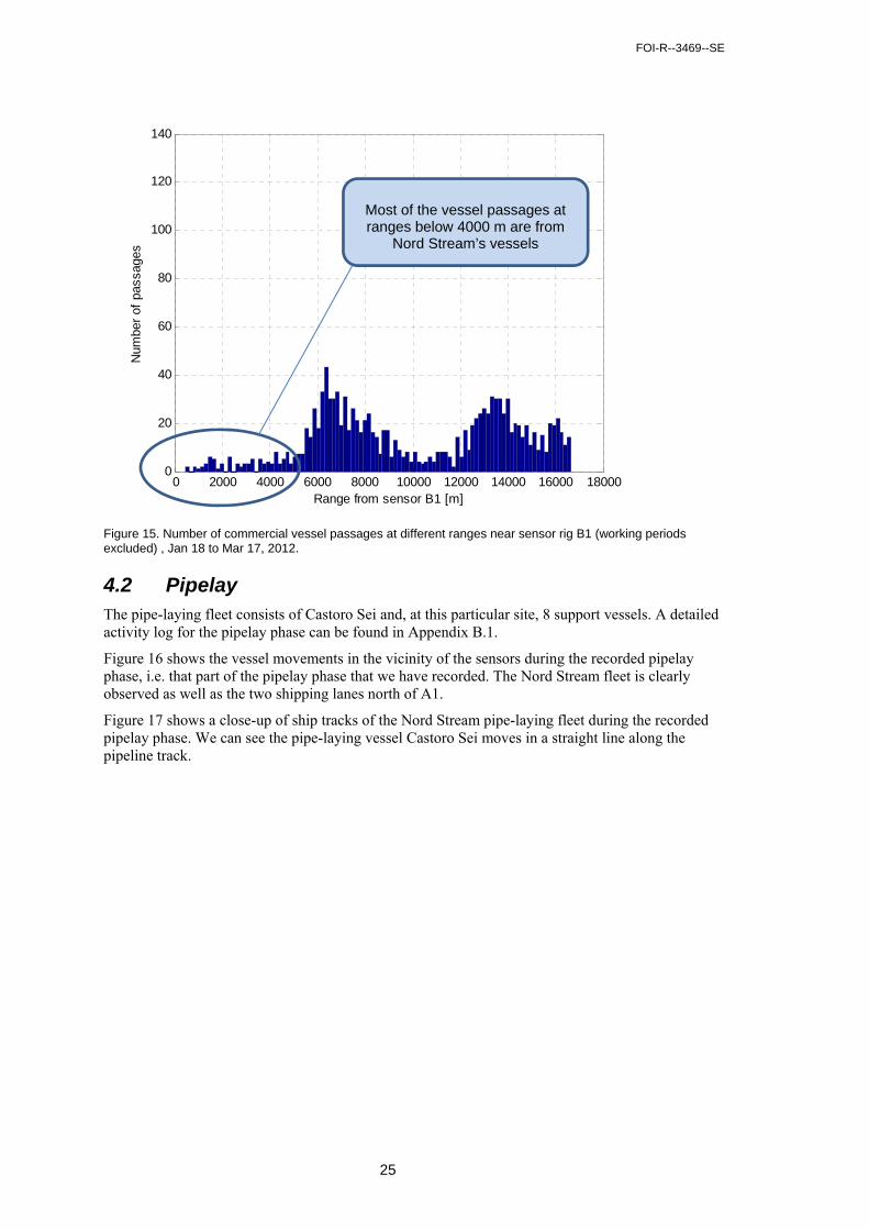
We also present vessel passages statistics for B1 for the same period as in Figure 14 except that the “working periods” were removed, see Figure 15. In this way we attempt to exclude Nord Stream’s vessels from the statistics. Comparing Figure 14 to Figure 15, we see that most of the passages at a range below 4000 m occur during the working periods. It is therefore likely that vessels passing within 4000 m of position B1 are mainly those of Nord Stream. The total number of passages during the measurement period except working periods at B1 was 97, leading to a daily average of 1.8.

FOI-R--3469--SE

24

Figure 13. Number of commercial vessel passages at different ranges near sensor rig A1 (near shipping lanes), Jan 18 to Mar 17, 2012.

Figure 14. Number of commercial vessel passages at different ranges near sensor rig B1 (near pipeline), Jan 18 to Mar 17, 2012.

0 2000 4000 6000 8000 10000 12000 14000 16000 180000

20

40

60

80

100

120

140

Range from sensor A1 [m]

Num

ber

of p

assa

ges

0 2000 4000 6000 8000 10000 12000 14000 16000 180000

20

40

60

80

100

120

140

Range from sensor B1 [m]

Num

ber

of p

assa

ges

FOI-R--3469--SE

25

Figure 15. Number of commercial vessel passages at different ranges near sensor rig B1 (working periods excluded) , Jan 18 to Mar 17, 2012.

4.2 Pipelay The pipe-laying fleet consists of Castoro Sei and, at this particular site, 8 support vessels. A detailed activity log for the pipelay phase can be found in Appendix B.1.

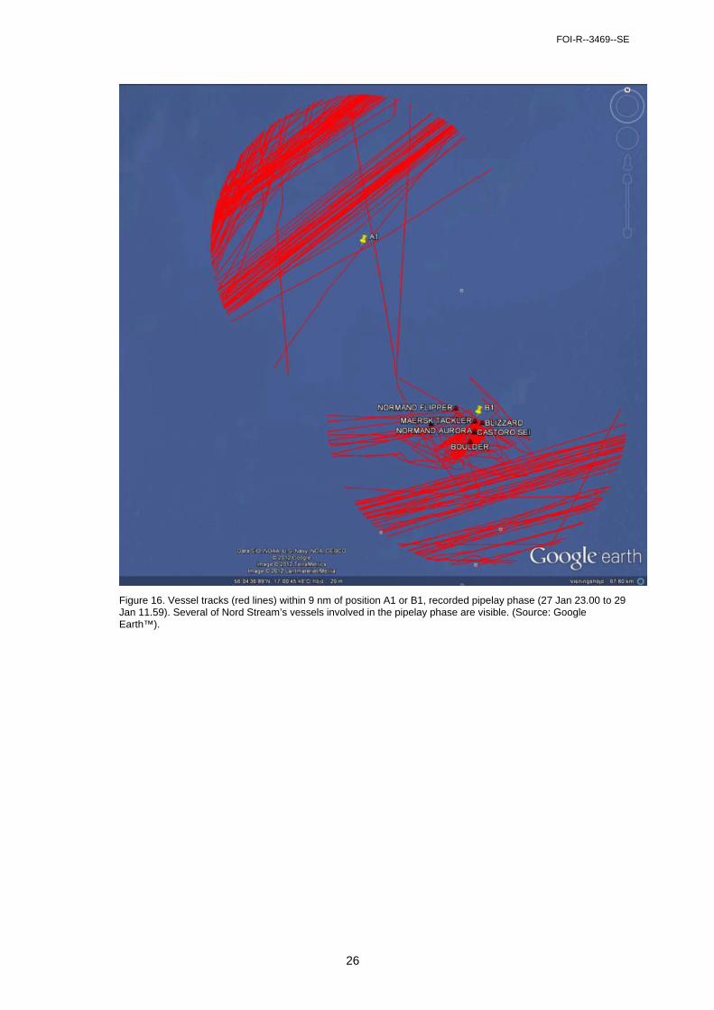
Figure 16 shows the vessel movements in the vicinity of the sensors during the recorded pipelay phase, i.e. that part of the pipelay phase that we have recorded. The Nord Stream fleet is clearly observed as well as the two shipping lanes north of A1.

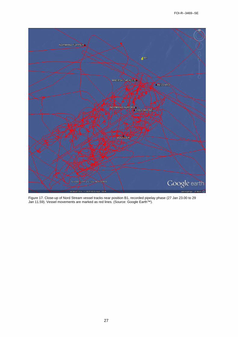
Figure 17 shows a close-up of ship tracks of the Nord Stream pipe-laying fleet during the recorded pipelay phase. We can see the pipe-laying vessel Castoro Sei moves in a straight line along the pipeline track.

0 2000 4000 6000 8000 10000 12000 14000 16000 180000

20

40

60

80

100

120

140

Range from sensor B1 [m]

Num

ber

of p

assa

ges

Most of the vessel passages at ranges below 4000 m are from

Nord Stream’s vessels

FOI-R--3469--SE

26

Figure 16. Vessel tracks (red lines) within 9 nm of position A1 or B1, recorded pipelay phase (27 Jan 23.00 to 29 Jan 11.59). Several of Nord Stream’s vessels involved in the pipelay phase are visible. (Source: Google Earth™).

FOI-R--3469--SE

27

Figure 17. Close-up of Nord Stream vessel tracks near position B1, recorded pipelay phase (27 Jan 23.00 to 29 Jan 11.59). Vessel movements are marked as red lines. (Source: Google Earth™).

FOI-R--3469--SE

28

4.3 Trenching The trenching at this site was performed by the vessel Far Samson (see Figure 2).

Figure 18 shows the vessel tracks in the vicinity of the sensors during the trenching phase. We can clearly see Far Samson and the two shipping lanes north of A1. Far Samson moves in a straight line along the pipeline track.

Figure 18. Vessel tracks (red lines) within 9 nm of position A1 or B1, trenching phase (25 Feb 20.00 to 26 Feb 19.08). (Source: Google Earth™).

FOI-R--3469--SE

29

5 Noise spectra and levels

5.1 Noise analysis methods In this report, we perform both a time series and a spectral analysis. A brief introduction to the acoustic terminology and units used here can be found in Appendix A.

The time series analysis studies the evolution of the total sound pressure. In Gerke (2011) the authors calculate the root-mean-square (RMS) pressure in 5 second intervals and present maximum, minimum and average RMS pressures in selected 1 minute intervals. They also calculate 24 hour averages as well as 24 hour 5th and 95th percentiles of the 5 s RMS pressure signals. For straightforward comparison to the Gerke’s results, we too use 5 second averaging and perform a similar analysis. Gerke (2011) measured and analysed noise levels in the German Bight during construction of the Nord Stream pipeline there in 2010, and so it is important to compare the results presented here to those of Gerke. This is done in Section 8.

Gerke (2011) and other references on noise levels use the standard arithmetic mean to estimate the average of a series of sound pressure level (SPL) values. This is calculated by summing the SPL values, expressed in µPa units, and dividing by the number of elements. To simplify a comparison with previous results, we use the same arithmetic mean throughout this report and simply call it the “mean” or the “average”. However, much of our data has outliers caused by nearby passages of loud commercial vessels, see e.g. Figure 23 at 28 Jan 12.00. For such data, the geometric mean gives a better representation of the average of the data series, where the centre of the distribution of values lies. The geometric mean can be calculated by multiplying the SPL values and taking the Nth root, where N is the number of data points. However, a simpler way to calculate it is to take the arithmetic mean of the SPL values expressed in logarithmic units (dB re 1 µPa). This also provides an intuitive interpretation of the geometric mean.

Through this report, if no qualifier is given, a “mean” or “average” value should be interpreted as an arithmetic mean. We mainly present arithmetic means, but tables of noise levels also present geometric means.

The spectral analysis studies the spectral levels at different times. Gerke (2011) studies the noise levels in third octave bands and presents averages. We will present similar results, but with more details on how the spectral levels vary in time. The edges of the third octave bands used here are given in Table 7.

Table 7. Third octave band edge frequencies (Hz).

11.2 14.1 17.8 22.4 28.2 35.5 44.7 56.2 70.8 89.1

112 141 178 224 282 355 447 562 708 891

1120 1410 1780 2240 2820 3550

In the frequency interval of interest (up to 2500 Hz), sea surface noise can contribute significantly to the ambient noise. Sea surface noise is generated by wind and waves and depends heavily on the weather. Therefore, it is important to compare noise levels to meteorological data. Data from a nearby weather station are presented in Section 3.1 and here we compare noise levels to this meteorological data.

The results from sensors A1 and A2 are similar. This is true also for sensors B1 and B2. Indeed, the main reason for having two sensors at the same place was redundancy; if one was lost or malfunctioned, the other would hopefully provide data. Therefore, in the interests of brevity, we only present results for sensors A1 and B1 here.

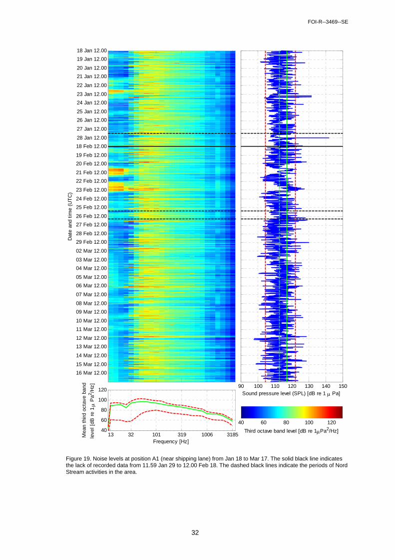
Throughout this section, noise levels are presented in full-page figures that attempt to demonstrate the full dynamics of the recorded noise. Each figure contains three sub-panels (see e.g. Figure 19).

The upper left panel presents the evolution of the third octave band spectrum. Time increases as we move downwards along the y-axis, which is marked with date and time stamps. Frequency is shown

FOI-R--3469--SE

30

on the x-axis, which is labelled by the mid frequencies of the third octave bands. Note that the sharp decrease in received levels above 3000 Hz is related to cut-off of the anti-aliasing filter. Thus, the unfiltered levels above 3000 Hz are most probably higher than those shown here. However, the filtering has a negligible effect on the sound pressure levels.

The upper right panel presents the evolution of the sound pressure level (SPL), i.e. the total sound pressure obtained by summing over the whole recorded frequency band of 0 to 3550 Hz. The pressure plot uses the same time axis as the third octave band graph. On the pressure plot, we see a number of vertical lines. These are

The (arithmetic) mean sound pressure level (solid green)

The geometric mean sound pressure level (dashed green)

The 5th and 95th percentile values (dashed red)

The percentile values are calculated by sorting the N pressure values and finding those values that are found at positions 0.05×N and 0.95×N, respectively, in the sorted data set.

The lower right hand plot presents the average third octave band spectrum (solid green line). 5th and 95th percentile spectra are indicated by dashed red lines.

5.2 Survey period overview To present an overview of the noise levels in the area, a 5 minute average third octave band spectrum and a 5 minute average sound pressure level (SPL) were calculated every 30 minutes. For the 5 minute files, averages were calculated for each file. For the 59 minute files, the first 5 minutes were extracted and averages were calculated. The same process was applied to data from 30 to 35 minutes into each 59 minute file. In this way, we obtain a long data series of 5 minute averages. (The results from analysis of the full 59 minute files will be presented in Section 5.3)

The results for sensor position A1 (near the shipping lane) are presented in Figure 19. The corresponding results for sensor position B1 (near the pipeline) are presented in Figure 20. In these figures, the time axis is discontinuous; the solid black line indicates the lack of recorded data from 11.59 Jan 29 to 12.00 Feb 18. Further, the dashed black lines indicate the periods of Nord Stream activities in the area.

In Figure 19 we see that the noise level at A1 (close to the shipping lanes) in the band 30 to 500 Hz varies at a time scale corresponding to hours. These variations can also be seen in the sound pressure levels. They are probably caused by noise radiated from passing vessels. In Section 6 we analyse a number of such passages.

The low frequency noise below 20 Hz is less than the cut-off frequency, thus stems from sources in close vicinity of the sensor. On Jan 23, Feb 21 and Feb 23 we see elevated levels at frequencies below 20 Hz. Comparing to the meteorological data presented in Section 3.1, we see that these dates correspond to peaks in the wind speed at levels of 12 to 18 m/s – periods of bad weather. It is therefore very likely that this low frequency noise is weather-related.

By visual inspection of the A1 noise levels, we see no apparent influence of Nord Stream’s activities or presence.

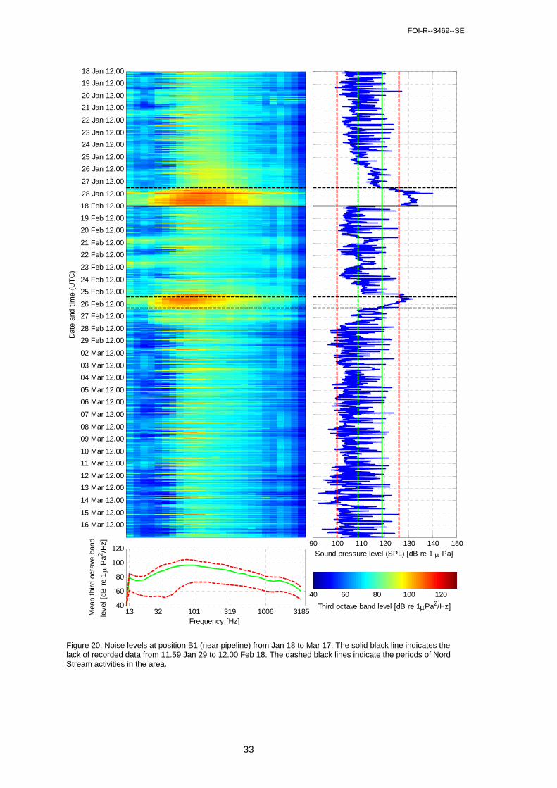
Comparing Figure 20 to Figure 19, we see that the levels between 30 and 500 Hz are lower at B1 than at A1, and that there is an increase in noise levels during pipelay and trenching. In Section 5.3 we analyse the noise levels further and compare to those radiated by vessels in the shipping lane near A1.

Comparing the average third octave band spectra at A1 and B1, we see higher levels at A1 below 100 Hz. In contrary, above 100 Hz, the average levels at B1 are higher.

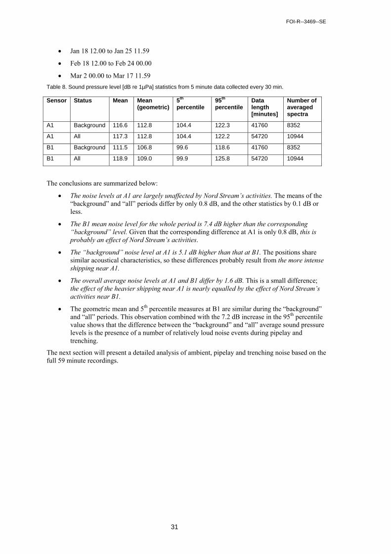
Table 8 presents the mean, geometric mean, 5th and 95th percentile of the 5 minute average sound pressure levels recorded at positions A1 and B1. The table presents results from “background” periods, i.e. all recordings taken when there were no Nord Stream vessels in the area, and from all the data. The following periods were classified as “background”:

FOI-R--3469--SE

31

Jan 18 12.00 to Jan 25 11.59

Feb 18 12.00 to Feb 24 00.00

Mar 2 00.00 to Mar 17 11.59

Table 8. Sound pressure level [dB re 1µPa] statistics from 5 minute data collected every 30 min.

Sensor Status Mean Mean (geometric)

5th

percentile 95th

percentile Data length [minutes]

Number of averaged spectra

A1 Background 116.6 112.8 104.4 122.3 41760 8352

A1 All 117.3 112.8 104.4 122.2 54720 10944

B1 Background 111.5 106.8 99.6 118.6 41760 8352

B1 All 118.9 109.0 99.9 125.8 54720 10944

The conclusions are summarized below:

The noise levels at A1 are largely unaffected by Nord Stream’s activities. The means of the “background” and “all” periods differ by only 0.8 dB, and the other statistics by 0.1 dB or less.

The B1 mean noise level for the whole period is 7.4 dB higher than the corresponding “background” level. Given that the corresponding difference at A1 is only 0.8 dB, this is probably an effect of Nord Stream’s activities.

The “background” noise level at A1 is 5.1 dB higher than that at B1. The positions share similar acoustical characteristics, so these differences probably result from the more intense shipping near A1.

The overall average noise levels at A1 and B1 differ by 1.6 dB. This is a small difference; the effect of the heavier shipping near A1 is nearly equalled by the effect of Nord Stream’s activities near B1.

The geometric mean and 5th percentile measures at B1 are similar during the “background” and “all” periods. This observation combined with the 7.2 dB increase in the 95th percentile value shows that the difference between the “background” and “all” average sound pressure levels is the presence of a number of relatively loud noise events during pipelay and trenching.

The next section will present a detailed analysis of ambient, pipelay and trenching noise based on the full 59 minute recordings.

FOI-R--3469--SE

32

Figure 19. Noise levels at position A1 (near shipping lane) from Jan 18 to Mar 17. The solid black line indicates the lack of recorded data from 11.59 Jan 29 to 12.00 Feb 18. The dashed black lines indicate the periods of Nord Stream activities in the area.

Dat

e an

d tim

e (U

TC

)

18 Jan 12.00

19 Jan 12.00

20 Jan 12.00

21 Jan 12.00

22 Jan 12.00

23 Jan 12.00

24 Jan 12.00

25 Jan 12.00

26 Jan 12.00

27 Jan 12.00

28 Jan 12.00

18 Feb 12.00

19 Feb 12.00

20 Feb 12.00

21 Feb 12.00

22 Feb 12.00

23 Feb 12.00

24 Feb 12.00

25 Feb 12.00

26 Feb 12.00

27 Feb 12.00

28 Feb 12.00

29 Feb 12.00

02 Mar 12.00

03 Mar 12.00

04 Mar 12.00

05 Mar 12.00

06 Mar 12.00

07 Mar 12.00

08 Mar 12.00

09 Mar 12.00

10 Mar 12.00

11 Mar 12.00

12 Mar 12.00

13 Mar 12.00

14 Mar 12.00

15 Mar 12.00

16 Mar 12.00

13 32 101 319 1006 318540

60

80

100

120

Frequency [Hz]

Mea

n th

ird o

ctav

e ba

nd

leve

l [dB

re

1

Pa2 /H

z]

40 60 80 100 120

Third octave band level [dB re 1Pa2/Hz]

90 100 110 120 130 140 150Sound pressure level (SPL) [dB re 1 Pa]

FOI-R--3469--SE

33

Figure 20. Noise levels at position B1 (near pipeline) from Jan 18 to Mar 17. The solid black line indicates the lack of recorded data from 11.59 Jan 29 to 12.00 Feb 18. The dashed black lines indicate the periods of Nord Stream activities in the area.

Dat

e an

d tim

e (U

TC

)18 Jan 12.00

19 Jan 12.00

20 Jan 12.00

21 Jan 12.00

22 Jan 12.00

23 Jan 12.00

24 Jan 12.00

25 Jan 12.00

26 Jan 12.00

27 Jan 12.00

28 Jan 12.00

18 Feb 12.00

19 Feb 12.00

20 Feb 12.00

21 Feb 12.00

22 Feb 12.00

23 Feb 12.00

24 Feb 12.00

25 Feb 12.00

26 Feb 12.00

27 Feb 12.00

28 Feb 12.00

29 Feb 12.00

02 Mar 12.00

03 Mar 12.00

04 Mar 12.00

05 Mar 12.00

06 Mar 12.00

07 Mar 12.00

08 Mar 12.00

09 Mar 12.00

10 Mar 12.00

11 Mar 12.00

12 Mar 12.00

13 Mar 12.00

14 Mar 12.00

15 Mar 12.00

16 Mar 12.00

13 32 101 319 1006 318540

60

80

100

120

Frequency [Hz]

Mea

n th

ird o

ctav

e ba

nd

leve

l [dB

re

1

Pa2 /H

z]

40 60 80 100 120

Third octave band level [dB re 1Pa2/Hz]

90 100 110 120 130 140 150Sound pressure level (SPL) [dB re 1 Pa]

FOI-R--3469--SE

34

5.3 Noise levels In the following sections we present measured noise levels during different time periods. These results are all based on the “nearly continuous” recordings taken during the first 59 minutes of every hour. For each recording, 5-second average power spectral densities were calculated. Noise levels are presented graphically in the same manner as in the previous section. The figures show both the temporal variations of the 5-second average levels and statistics on these variations.

We commence by studying the ambient noise levels and limit our attention to a period when no Nord Stream vessels were in the vicinity of our sensors. After the ambient noise has been analysed, we turn the attention to noise levels during Nord Stream’s activities. First we describe the noise measured during pipelay, and then that found during trenching.

5.3.1 Ambient noise

Nearly continuous recordings are available from 25 to 29 January. During most of this period, Nord Stream vessels were in the Norra Midsjöbanken area. Therefore this data does not provide a good representation of the ambient noise in the area.

There are also nearly continuous recordings from 25 February until 6 Mar. From Mar 2 until Mar 6, there are no Nord Stream vessels in the area. Therefore, the data recorded during that period can be said to consist only of ambient noise.

During the interval 00.00 Mar 2 to 11.59 Mar 6 the wind speed ranged from 2 to 9 m/s. The average was 5.2 m/s.

Figure 21 presents noise levels at A1. Comparing to the noise levels at B1 (Figure 22), we note again the higher number of loud vessel passages at A1. The mean third octave band levels at A1 are higher than at B1 at all frequencies. Between 20 and 1500 Hz, the difference is at least 4 dB.

Table 9 presents sound pressure level statistics for the background period.

Table 9. Sound pressure level (dB re 1 µPa) statistics for 00.00 Mar 2 to 11.59 Mar 6 – background.

Sensor Status Mean Mean (geometric)

5th

percentile 95th

percentile Data length (minutes)

Number of averaged spectra

A1 Background 116.5 113.0 104.3 122.0 6372 76464

B1 Background 110.9 106.1 99.2 116.6 6372 76464

The following conclusions are made:

The average ambient noise level at A1 is 5.6 dB higher than that at B1. The positions share similar acoustical characteristics, thus these differences probably result from the more intense shipping near A1. (In Section 5.2, we found a corresponding difference of 5.1 dB for the 5 minute background recordings. The 0.5 dB discrepancy is small and can be caused by variations in vessel traffic intensity.)

The 5th and 95th percentile levels are also higher at A1 than at B1. This means that the loudest intervals are louder at A1, and the quietest intervals are not as quiet as at B1. This can also be seen by comparing the sound pressure level data in Figure 21 and Figure 22.

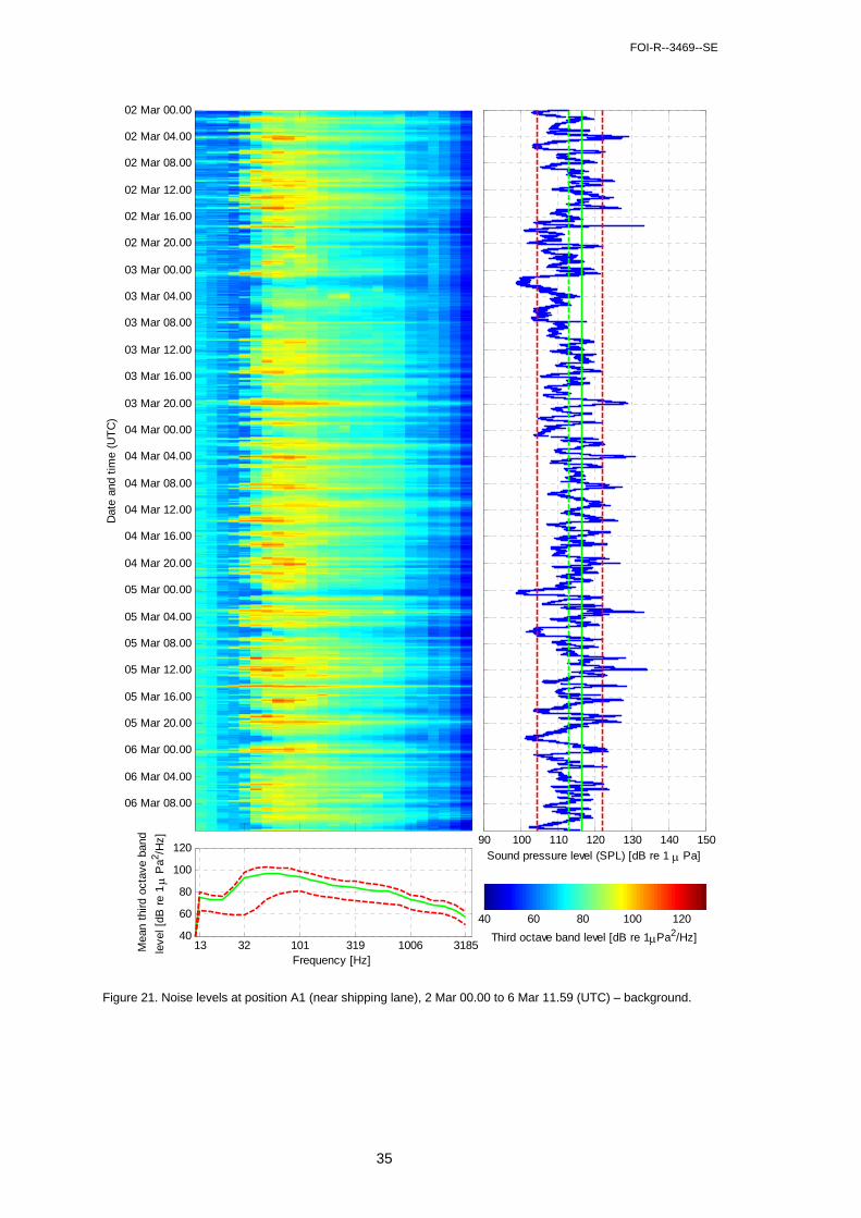
FOI-R--3469--SE

35

Figure 21. Noise levels at position A1 (near shipping lane), 2 Mar 00.00 to 6 Mar 11.59 (UTC) – background.

Dat

e an

d tim

e (U

TC

)02 Mar 00.00

02 Mar 04.00

02 Mar 08.00

02 Mar 12.00

02 Mar 16.00

02 Mar 20.00

03 Mar 00.00

03 Mar 04.00

03 Mar 08.00

03 Mar 12.00

03 Mar 16.00

03 Mar 20.00

04 Mar 00.00

04 Mar 04.00

04 Mar 08.00

04 Mar 12.00

04 Mar 16.00

04 Mar 20.00

05 Mar 00.00

05 Mar 04.00

05 Mar 08.00

05 Mar 12.00

05 Mar 16.00

05 Mar 20.00

06 Mar 00.00

06 Mar 04.00

06 Mar 08.00

13 32 101 319 1006 318540

60

80

100

120

Frequency [Hz]

Mea

n th

ird o

ctav

e ba

nd

leve

l [dB

re

1

Pa2 /H

z]

40 60 80 100 120

Third octave band level [dB re 1Pa2/Hz]

90 100 110 120 130 140 150Sound pressure level (SPL) [dB re 1 Pa]

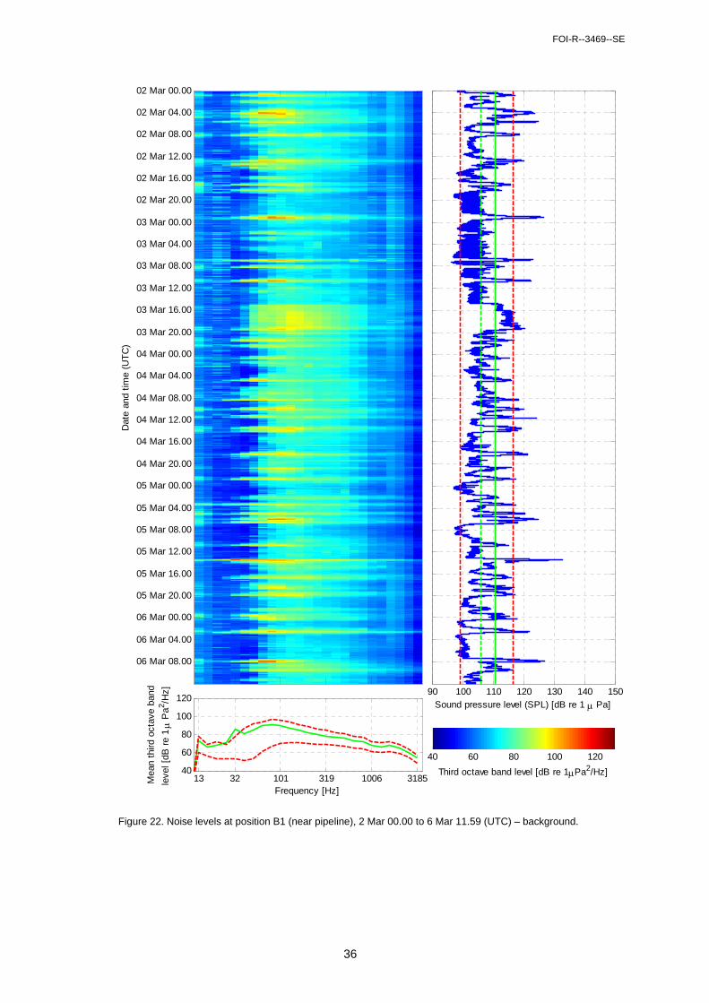
FOI-R--3469--SE

36

Figure 22. Noise levels at position B1 (near pipeline), 2 Mar 00.00 to 6 Mar 11.59 (UTC) – background.

Dat

e an

d tim

e (U

TC

)

02 Mar 00.00

02 Mar 04.00

02 Mar 08.00

02 Mar 12.00

02 Mar 16.00

02 Mar 20.00

03 Mar 00.00

03 Mar 04.00

03 Mar 08.00

03 Mar 12.00

03 Mar 16.00

03 Mar 20.00

04 Mar 00.00

04 Mar 04.00

04 Mar 08.00

04 Mar 12.00

04 Mar 16.00

04 Mar 20.00

05 Mar 00.00

05 Mar 04.00

05 Mar 08.00

05 Mar 12.00

05 Mar 16.00

05 Mar 20.00

06 Mar 00.00

06 Mar 04.00

06 Mar 08.00

13 32 101 319 1006 318540

60

80

100

120

Frequency [Hz]

Mea

n th

ird o

ctav

e ba

nd

leve

l [dB

re

1

Pa2 /H

z]

40 60 80 100 120

Third octave band level [dB re 1Pa2/Hz]

90 100 110 120 130 140 150Sound pressure level (SPL) [dB re 1 Pa]

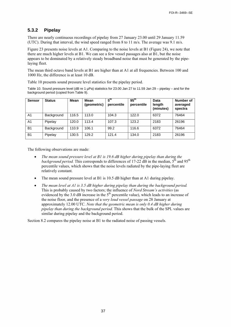
FOI-R--3469--SE

37

5.3.2 Pipelay

There are nearly continuous recordings of pipelay from 27 January 23.00 until 29 January 11.59 (UTC). During that interval, the wind speed ranged from 8 to 11 m/s. The average was 9.1 m/s.

Figure 23 presents noise levels at A1. Comparing to the noise levels at B1 (Figure 24), we note that there are much higher levels at B1. We can see a few vessel passages also at B1, but the noise appears to be dominated by a relatively steady broadband noise that must be generated by the pipe-laying fleet.

The mean third octave band levels at B1 are higher than at A1 at all frequencies. Between 100 and 1000 Hz, the difference is at least 10 dB.

Table 10 presents sound pressure level statistics for the pipelay period.

Table 10. Sound pressure level (dB re 1 µPa) statistics for 23.00 Jan 27 to 11.59 Jan 29 – pipelay – and for the background period (copied from Table 9).

Sensor Status Mean Mean (geometric)

5th

percentile 95th

percentile Data length (minutes)

Number of averaged spectra

A1 Background 116.5 113.0 104.3 122.0 6372 76464

A1 Pipelay 120.0 113.4 107.3 123.2 2183 26196

B1 Background 110.9 106.1 99.2 116.6 6372 76464

B1 Pipelay 130.5 129.2 121.4 134.0 2183 26196

The following observations are made:

The mean sound pressure level at B1 is 19.6 dB higher during pipelay than during the background period. This corresponds to differences of 17-22 dB in the median, 5th and 95th percentile values, which shows that the noise levels radiated by the pipe-laying fleet are relatively constant.

The mean sound pressure level at B1 is 10.5 dB higher than at A1 during pipelay.

The mean level at A1 is 3.5 dB higher during pipelay than during the background period. This is probably caused by two factors; the influence of Nord Stream’s activities (as evidenced by the 3.0 dB increase in the 5th percentile value), which leads to an increase of the noise floor, and the presence of a very loud vessel passage on 28 January at approximately 12.00 UTC. Note that the geometric mean is only 0.4 dB higher during pipelay than during the background period. This shows that the bulk of the SPL values are similar during pipelay and the background period.

Section 8.2 compares the pipelay noise at B1 to the radiated noise of passing vessels.

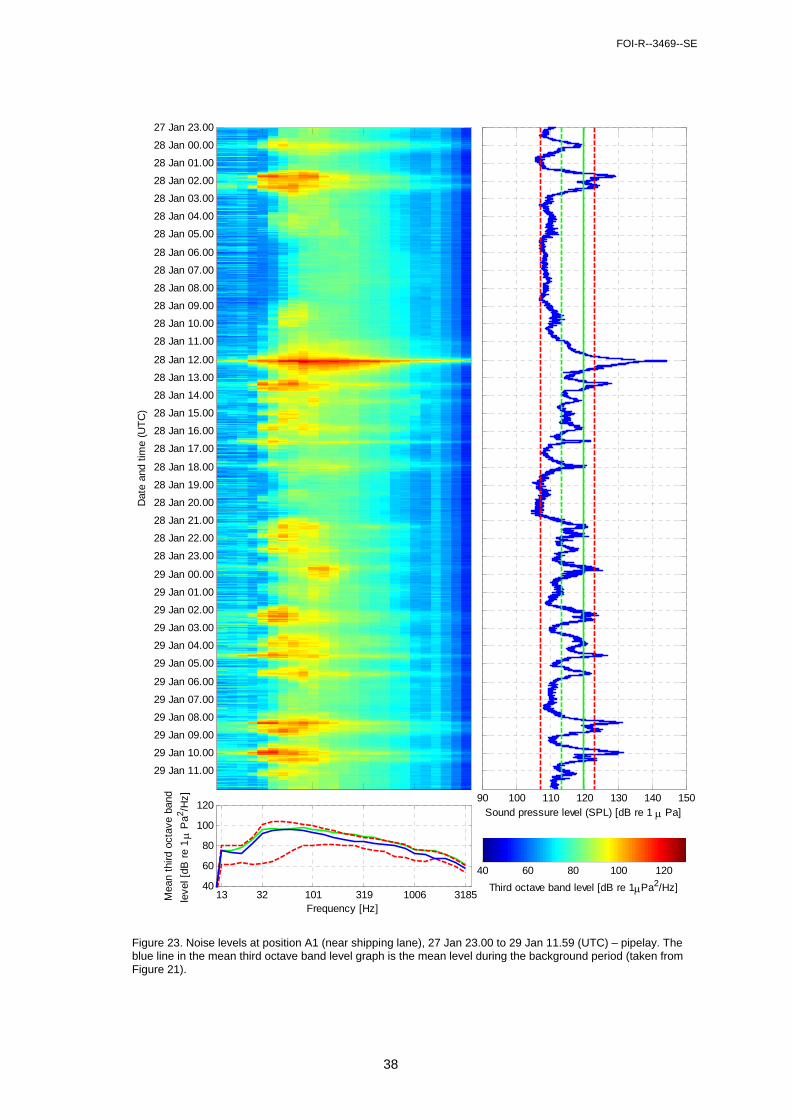
FOI-R--3469--SE

38

Figure 23. Noise levels at position A1 (near shipping lane), 27 Jan 23.00 to 29 Jan 11.59 (UTC) – pipelay. The blue line in the mean third octave band level graph is the mean level during the background period (taken from Figure 21).

Dat

e an

d tim

e (U

TC

)27 Jan 23.00

28 Jan 00.00

28 Jan 01.00

28 Jan 02.00

28 Jan 03.00

28 Jan 04.00

28 Jan 05.00

28 Jan 06.00

28 Jan 07.00

28 Jan 08.00

28 Jan 09.00

28 Jan 10.00

28 Jan 11.00

28 Jan 12.00

28 Jan 13.00

28 Jan 14.00

28 Jan 15.00

28 Jan 16.00

28 Jan 17.00

28 Jan 18.00

28 Jan 19.00

28 Jan 20.00

28 Jan 21.00

28 Jan 22.00

28 Jan 23.00

29 Jan 00.00

29 Jan 01.00

29 Jan 02.00

29 Jan 03.00

29 Jan 04.00

29 Jan 05.00

29 Jan 06.00

29 Jan 07.00

29 Jan 08.00

29 Jan 09.00

29 Jan 10.00

29 Jan 11.00

13 32 101 319 1006 318540

60

80

100

120

Frequency [Hz]

Mea

n th

ird o

ctav

e ba

nd

leve

l [dB

re

1

Pa2 /H

z]

40 60 80 100 120

Third octave band level [dB re 1Pa2/Hz]

90 100 110 120 130 140 150Sound pressure level (SPL) [dB re 1 Pa]

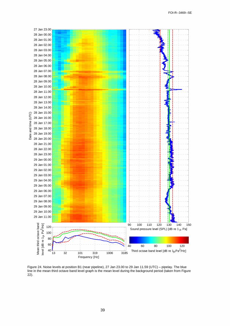
FOI-R--3469--SE

39

Figure 24. Noise levels at position B1 (near pipeline), 27 Jan 23.00 to 29 Jan 11.59 (UTC) – pipelay. The blue line in the mean third octave band level graph is the mean level during the background period (taken from Figure 22).

Dat

e an

d tim

e (U

TC

)27 Jan 23.00

28 Jan 00.00

28 Jan 01.00

28 Jan 02.00

28 Jan 03.00

28 Jan 04.00

28 Jan 05.00

28 Jan 06.00

28 Jan 07.00

28 Jan 08.00

28 Jan 09.00

28 Jan 10.00

28 Jan 11.00

28 Jan 12.00

28 Jan 13.00

28 Jan 14.00

28 Jan 15.00

28 Jan 16.00

28 Jan 17.00

28 Jan 18.00

28 Jan 19.00

28 Jan 20.00

28 Jan 21.00

28 Jan 22.00

28 Jan 23.00

29 Jan 00.00

29 Jan 01.00

29 Jan 02.00

29 Jan 03.00

29 Jan 04.00

29 Jan 05.00

29 Jan 06.00

29 Jan 07.00

29 Jan 08.00

29 Jan 09.00

29 Jan 10.00

29 Jan 11.00

13 32 101 319 1006 318540

60

80

100

120

Frequency [Hz]

Mea

n th

ird o

ctav

e ba

nd

leve

l [dB

re

1

Pa2 /H

z]

40 60 80 100 120

Third octave band level [dB re 1Pa2/Hz]

90 100 110 120 130 140 150Sound pressure level (SPL) [dB re 1 Pa]

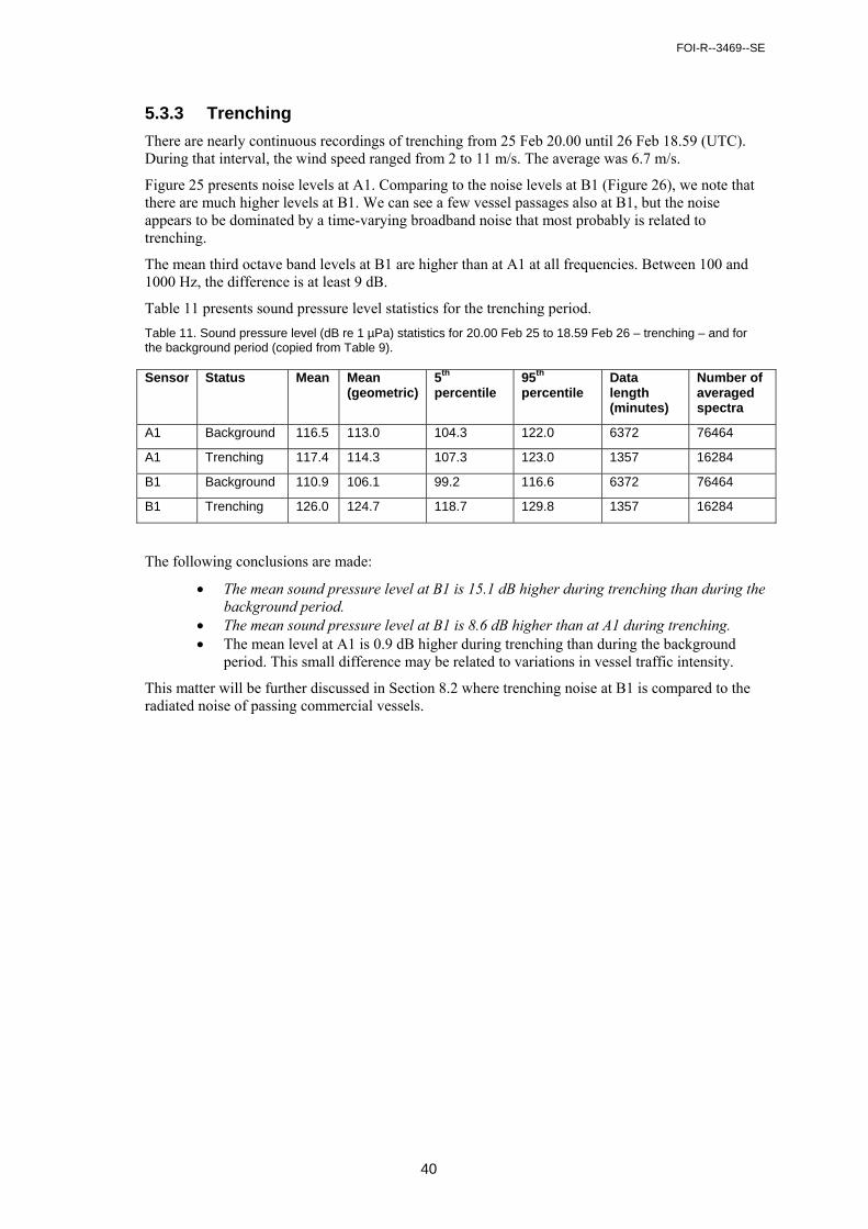
FOI-R--3469--SE

40

5.3.3 Trenching

There are nearly continuous recordings of trenching from 25 Feb 20.00 until 26 Feb 18.59 (UTC). During that interval, the wind speed ranged from 2 to 11 m/s. The average was 6.7 m/s.

Figure 25 presents noise levels at A1. Comparing to the noise levels at B1 (Figure 26), we note that there are much higher levels at B1. We can see a few vessel passages also at B1, but the noise appears to be dominated by a time-varying broadband noise that most probably is related to trenching.

The mean third octave band levels at B1 are higher than at A1 at all frequencies. Between 100 and 1000 Hz, the difference is at least 9 dB.

Table 11 presents sound pressure level statistics for the trenching period.

Table 11. Sound pressure level (dB re 1 µPa) statistics for 20.00 Feb 25 to 18.59 Feb 26 – trenching – and for the background period (copied from Table 9).

Sensor Status Mean Mean (geometric)

5th

percentile 95th

percentile Data length (minutes)

Number of averaged spectra

A1 Background 116.5 113.0 104.3 122.0 6372 76464

A1 Trenching 117.4 114.3 107.3 123.0 1357 16284

B1 Background 110.9 106.1 99.2 116.6 6372 76464

B1 Trenching 126.0 124.7 118.7 129.8 1357 16284

The following conclusions are made:

The mean sound pressure level at B1 is 15.1 dB higher during trenching than during the background period.

The mean sound pressure level at B1 is 8.6 dB higher than at A1 during trenching. The mean level at A1 is 0.9 dB higher during trenching than during the background

period. This small difference may be related to variations in vessel traffic intensity.

This matter will be further discussed in Section 8.2 where trenching noise at B1 is compared to the radiated noise of passing commercial vessels.

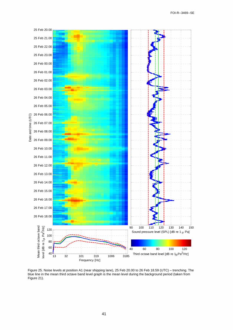
FOI-R--3469--SE

41

Figure 25. Noise levels at position A1 (near shipping lane), 25 Feb 20.00 to 26 Feb 18.59 (UTC) – trenching. The blue line in the mean third octave band level graph is the mean level during the background period (taken from Figure 21).

Dat

e an

d tim

e (U

TC

)25 Feb 20.00

25 Feb 21.00

25 Feb 22.00

25 Feb 23.00

26 Feb 00.00

26 Feb 01.00

26 Feb 02.00

26 Feb 03.00

26 Feb 04.00

26 Feb 05.00

26 Feb 06.00

26 Feb 07.00

26 Feb 08.00

26 Feb 09.00

26 Feb 10.00

26 Feb 11.00

26 Feb 12.00

26 Feb 13.00

26 Feb 14.00

26 Feb 15.00

26 Feb 16.00

26 Feb 17.00

26 Feb 18.00

13 32 101 319 1006 318540

60

80

100

120

Frequency [Hz]

Mea

n th

ird o

ctav

e ba

nd

leve

l [dB

re

1

Pa2 /H

z]

40 60 80 100 120

Third octave band level [dB re 1Pa2/Hz]

90 100 110 120 130 140 150Sound pressure level (SPL) [dB re 1 Pa]

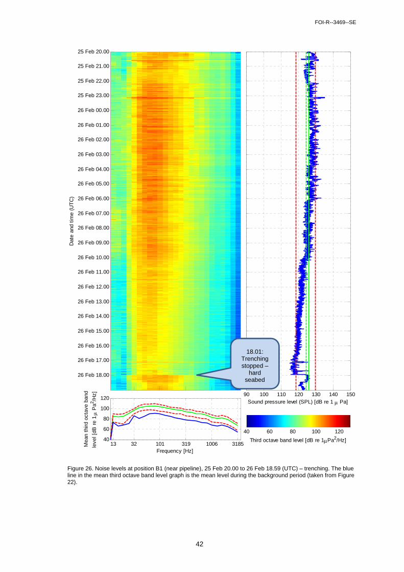
FOI-R--3469--SE

42

Figure 26. Noise levels at position B1 (near pipeline), 25 Feb 20.00 to 26 Feb 18.59 (UTC) – trenching. The blue line in the mean third octave band level graph is the mean level during the background period (taken from Figure 22).

Dat

e an

d tim

e (U

TC

)

25 Feb 20.00

25 Feb 21.00

25 Feb 22.00

25 Feb 23.00

26 Feb 00.00

26 Feb 01.00

26 Feb 02.00

26 Feb 03.00

26 Feb 04.00

26 Feb 05.00

26 Feb 06.00

26 Feb 07.00

26 Feb 08.00

26 Feb 09.00

26 Feb 10.00

26 Feb 11.00

26 Feb 12.00

26 Feb 13.00

26 Feb 14.00

26 Feb 15.00

26 Feb 16.00

26 Feb 17.00

26 Feb 18.00

13 32 101 319 1006 318540

60

80

100

120

Frequency [Hz]

Mea

n th

ird o

ctav

e ba

nd

leve

l [dB

re

1

Pa2 /H

z]

40 60 80 100 120

Third octave band level [dB re 1Pa2/Hz]

90 100 110 120 130 140 150Sound pressure level (SPL) [dB re 1 Pa]

18.01: Trenching stopped –

hard seabed

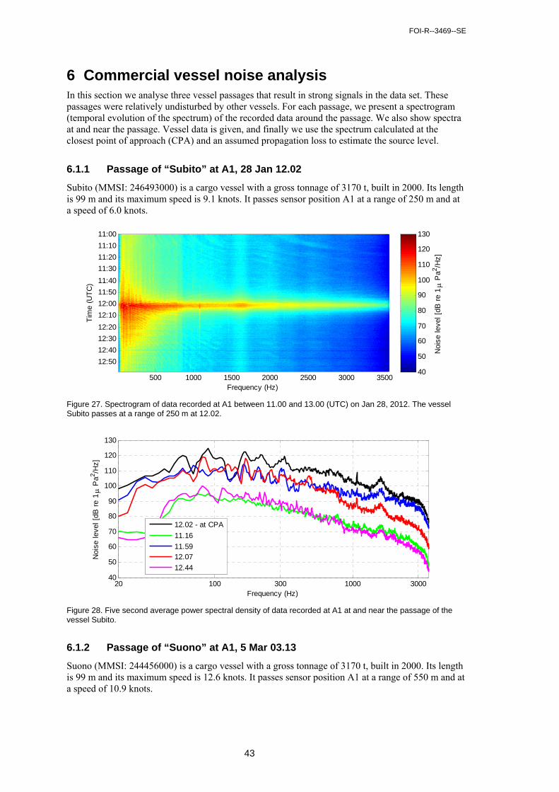
FOI-R--3469--SE

43

6 Commercial vessel noise analysis In this section we analyse three vessel passages that result in strong signals in the data set. These passages were relatively undisturbed by other vessels. For each passage, we present a spectrogram (temporal evolution of the spectrum) of the recorded data around the passage. We also show spectra at and near the passage. Vessel data is given, and finally we use the spectrum calculated at the closest point of approach (CPA) and an assumed propagation loss to estimate the source level.

6.1.1 Passage of “Subito” at A1, 28 Jan 12.02

Subito (MMSI: 246493000) is a cargo vessel with a gross tonnage of 3170 t, built in 2000. Its length is 99 m and its maximum speed is 9.1 knots. It passes sensor position A1 at a range of 250 m and at a speed of 6.0 knots.

Figure 27. Spectrogram of data recorded at A1 between 11.00 and 13.00 (UTC) on Jan 28, 2012. The vessel Subito passes at a range of 250 m at 12.02.

Figure 28. Five second average power spectral density of data recorded at A1 at and near the passage of the vessel Subito.

6.1.2 Passage of “Suono” at A1, 5 Mar 03.13

Suono (MMSI: 244456000) is a cargo vessel with a gross tonnage of 3170 t, built in 2000. Its length is 99 m and its maximum speed is 12.6 knots. It passes sensor position A1 at a range of 550 m and at a speed of 10.9 knots.

Frequency (Hz)

Tim

e (U

TC

)

500 1000 1500 2000 2500 3000 3500

11:00

11:10

11:20

11:30

11:40

11:50

12:00

12:10

12:20

12:30

12:40

12:50

Noi

se le

vel [

dB r

e 1

Pa2 /H

z]

40

50

60

70

80

90

100

110

120

130

20 100 300 1000 300040

50

60

70

80

90

100

110

120

130

Frequency (Hz)

Noi

se le

vel [

dB r

e 1

Pa2 /H

z]

12.02 - at CPA

11.16

11.5912.07

12.44

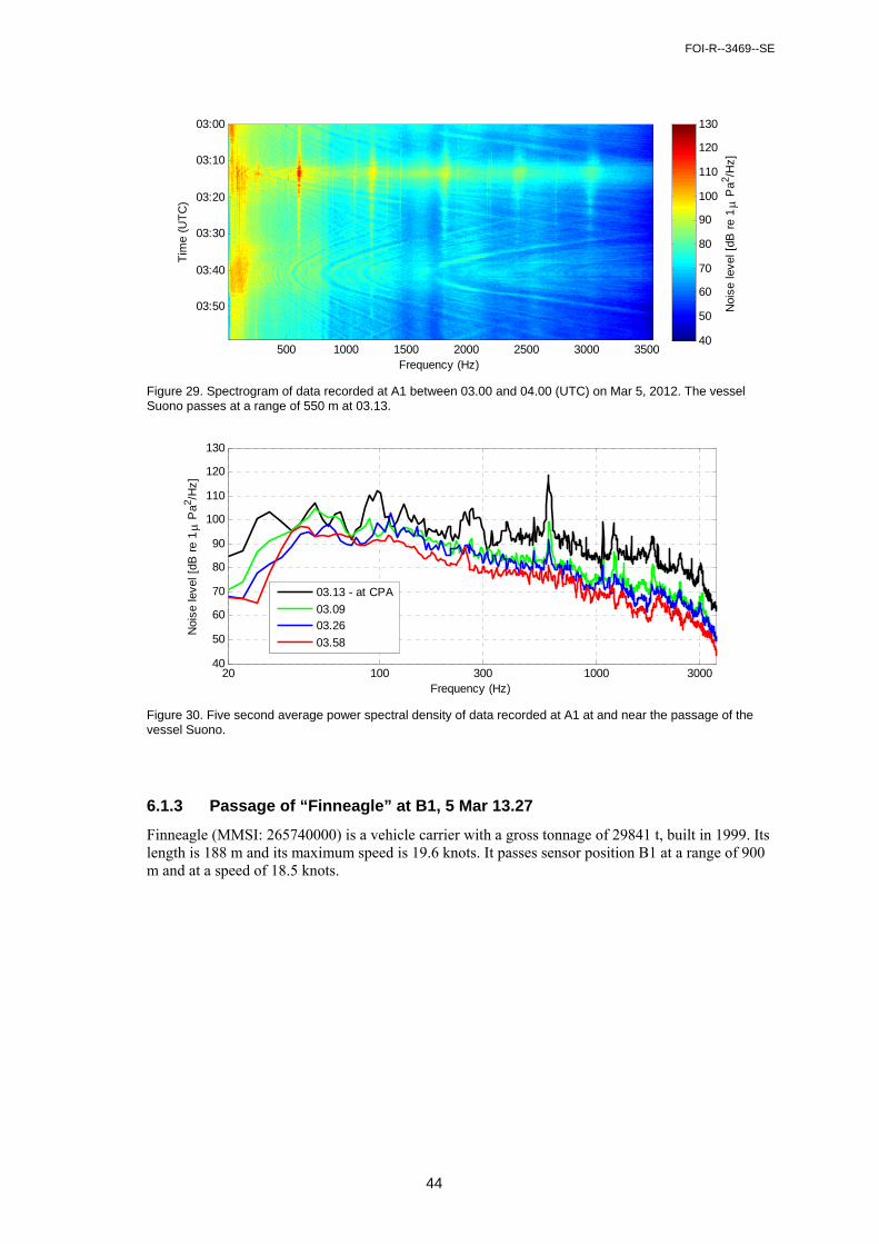
FOI-R--3469--SE

44

Figure 29. Spectrogram of data recorded at A1 between 03.00 and 04.00 (UTC) on Mar 5, 2012. The vessel Suono passes at a range of 550 m at 03.13.

Figure 30. Five second average power spectral density of data recorded at A1 at and near the passage of the vessel Suono.

6.1.3 Passage of “Finneagle” at B1, 5 Mar 13.27

Finneagle (MMSI: 265740000) is a vehicle carrier with a gross tonnage of 29841 t, built in 1999. Its length is 188 m and its maximum speed is 19.6 knots. It passes sensor position B1 at a range of 900 m and at a speed of 18.5 knots.

Frequency (Hz)

Tim

e (U

TC

)

500 1000 1500 2000 2500 3000 3500

03:00

03:10

03:20

03:30

03:40

03:50 Noi

se le

vel [

dB r

e 1

Pa2 /H

z]

40

50

60

70

80

90

100

110

120

130

20 100 300 1000 300040

50

60

70

80

90

100

110

120

130

Frequency (Hz)

Noi

se le

vel [

dB r

e 1

Pa2 /H

z]

03.13 - at CPA

03.0903.26

03.58

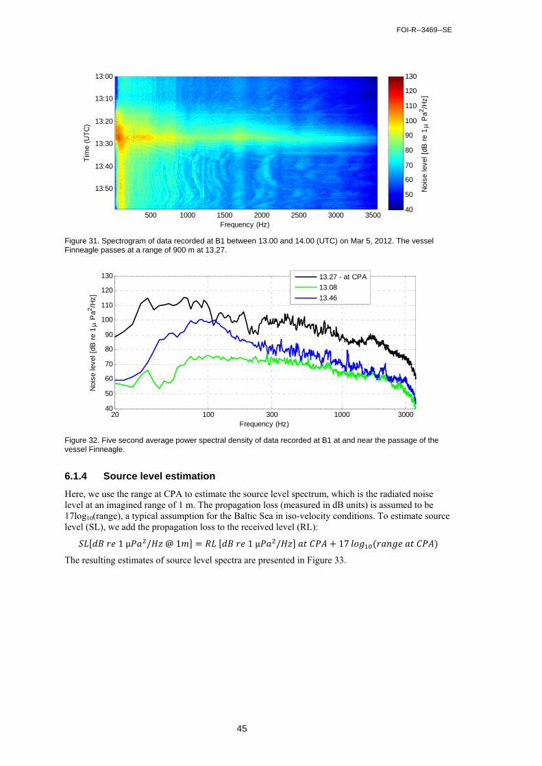
FOI-R--3469--SE

45

Figure 31. Spectrogram of data recorded at B1 between 13.00 and 14.00 (UTC) on Mar 5, 2012. The vessel Finneagle passes at a range of 900 m at 13.27.

Figure 32. Five second average power spectral density of data recorded at B1 at and near the passage of the vessel Finneagle.

6.1.4 Source level estimation

Here, we use the range at CPA to estimate the source level spectrum, which is the radiated noise level at an imagined range of 1 m. The propagation loss (measured in dB units) is assumed to be 17log10(range), a typical assumption for the Baltic Sea in iso-velocity conditions. To estimate source level (SL), we add the propagation loss to the received level (RL):

1μ / @1 1μ / 17

The resulting estimates of source level spectra are presented in Figure 33.

Frequency (Hz)

Tim

e (U

TC

)

500 1000 1500 2000 2500 3000 3500

13:00

13:10

13:20

13:30

13:40

13:50 Noi

se le

vel [

dB r

e 1

Pa2 /H

z]

40

50

60

70

80

90

100

110

120

130

20 100 300 1000 300040

50

60

70

80

90

100

110

120

130

Frequency (Hz)

Noi

se le

vel [

dB r

e 1

Pa2 /H

z]

13.27 - at CPA

13.08

13.46

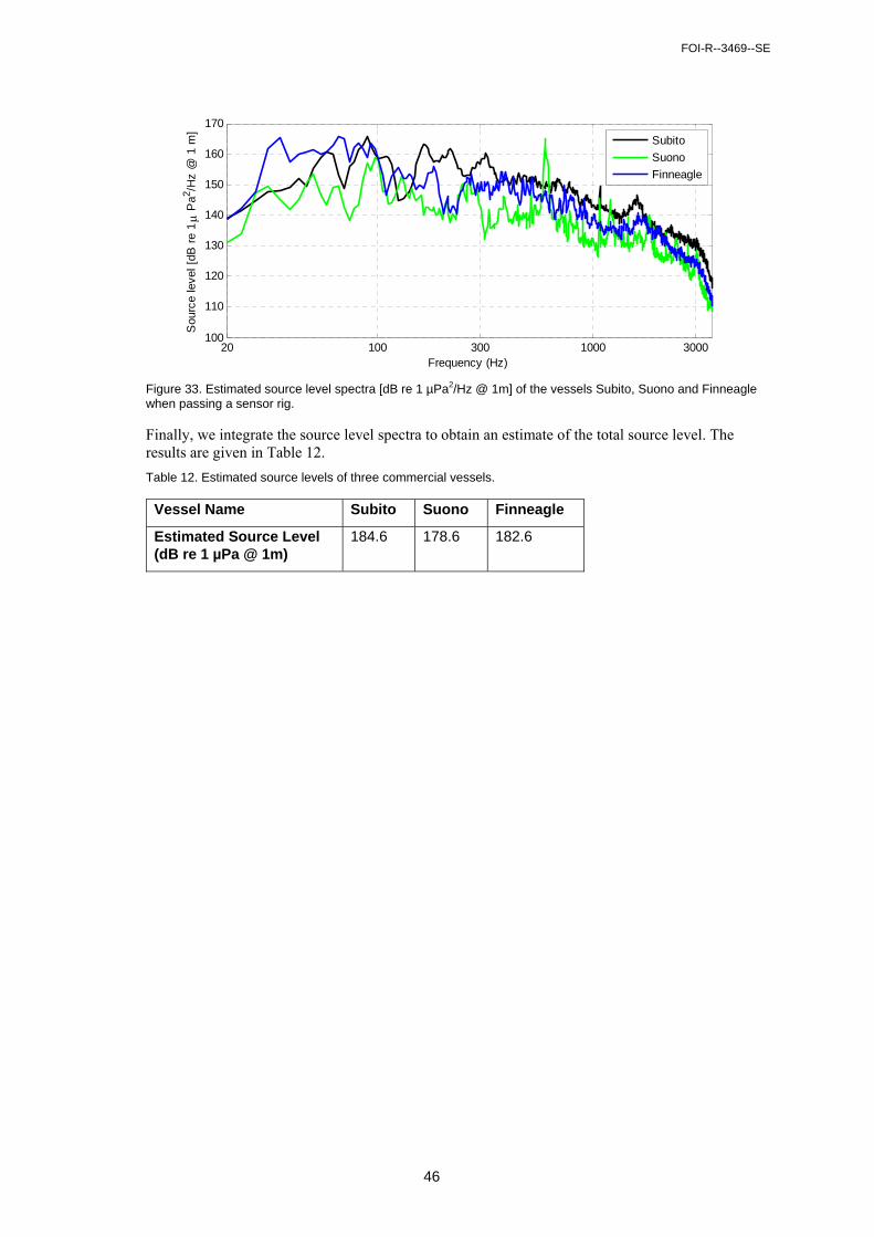
FOI-R--3469--SE

46

Figure 33. Estimated source level spectra [dB re 1 µPa2/Hz @ 1m] of the vessels Subito, Suono and Finneagle when passing a sensor rig.

Finally, we integrate the source level spectra to obtain an estimate of the total source level. The results are given in Table 12.

Table 12. Estimated source levels of three commercial vessels.

Vessel Name Subito Suono Finneagle

Estimated Source Level (dB re 1 µPa @ 1m)

184.6 178.6 182.6

20 100 300 1000 3000100

110

120

130

140

150

160

170

Frequency (Hz)

Sou

rce

leve

l [dB

re

1

Pa2 /H

z @

1 m

]

Subito

Suono

Finneagle

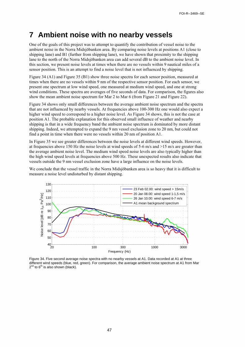
FOI-R--3469--SE

47

7 Ambient noise with no nearby vessels One of the goals of this project was to attempt to quantify the contribution of vessel noise to the ambient noise in the Norra Midsjöbanken area. By comparing noise levels at positions A1 (close to shipping lane) and B1 (further from shipping lane), we have shown that proximity to the shipping lane to the north of the Norra Midsjöbanken area can add several dB to the ambient noise level. In this section, we present noise levels at times when there are no vessels within 9 nautical miles of a sensor position. This is an attempt to find a noise level that is not influenced by shipping.

Figure 34 (A1) and Figure 35 (B1) show three noise spectra for each sensor position, measured at times when there are no vessels within 9 nm of the respective sensor position. For each sensor, we present one spectrum at low wind speed, one measured at medium wind speed, and one at strong wind conditions. These spectra are averages of five seconds of data. For comparison, the figures also show the mean ambient noise spectrum for Mar 2 to Mar 6 (from Figure 21 and Figure 22).

Figure 34 shows only small differences between the average ambient noise spectrum and the spectra that are not influenced by nearby vessels. At frequencies above 100-300 Hz one would also expect a higher wind speed to correspond to a higher noise level. As Figure 34 shows, this is not the case at position A1. The probable explanation for this observed small influence of weather and nearby shipping is that in a wide frequency band the ambient noise spectrum is dominated by more distant shipping. Indeed, we attempted to expand the 9 nm vessel exclusion zone to 20 nm, but could not find a point in time when there were no vessels within 20 nm of position A1.

In Figure 35 we see greater differences between the noise levels at different wind speeds. However, at frequencies above 150 Hz the noise levels at wind speeds of 5-6 m/s and >15 m/s are greater than the average ambient noise level. The medium wind speed noise levels are also typically higher than the high wind speed levels at frequencies above 500 Hz. These unexpected results also indicate that vessels outside the 9 nm vessel exclusion zone have a large influence on the noise levels.

We conclude that the vessel traffic in the Norra Midsjöbanken area is so heavy that it is difficult to measure a noise level undisturbed by distant shipping.

Figure 34. Five second average noise spectra with no nearby vessels at A1. Data recorded at A1 at three different wind speeds (blue, red, green). For comparison, the average ambient noise spectrum at A1 from Mar 2nd to 6th is also shown (black).

20 100 300 1000 300040

50

60

70

80

90

100

110

120

130

Frequency (Hz)

Noi

se le

vel [

dB r

e 1

Pa2 /H

z]

23 Feb 02.00: wind speed > 15m/s

20 Jan 08.00: wind speed 1-1,5 m/s26 Jan 10.00: wind speed 6-7 m/s

A1 mean background spectrum

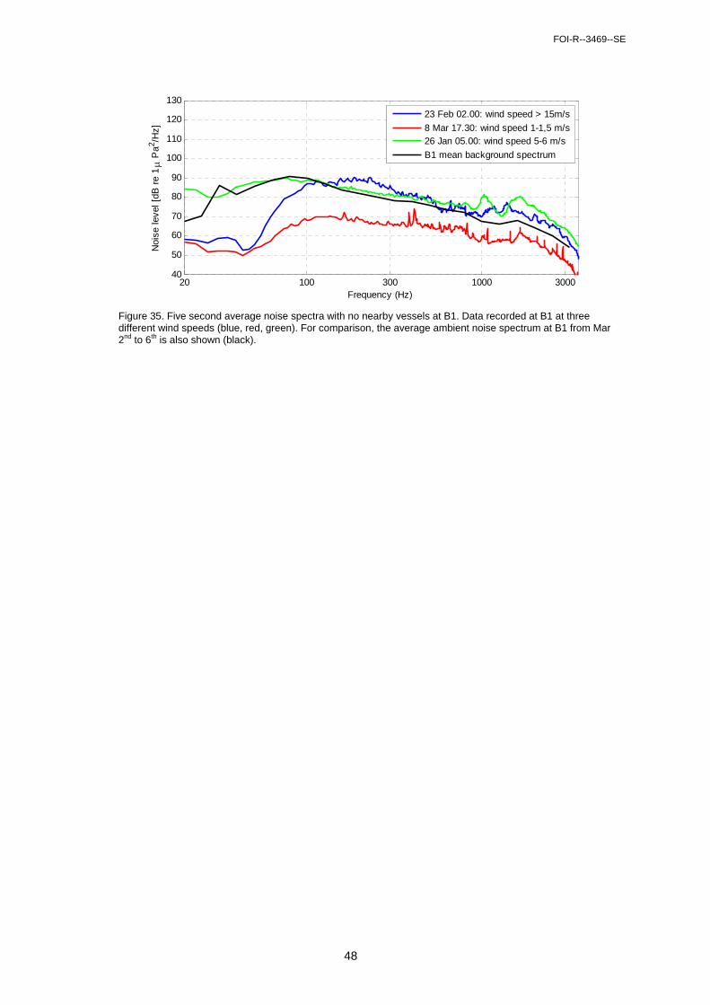
FOI-R--3469--SE

48

Figure 35. Five second average noise spectra with no nearby vessels at B1. Data recorded at B1 at three different wind speeds (blue, red, green). For comparison, the average ambient noise spectrum at B1 from Mar 2nd to 6th is also shown (black).

20 100 300 1000 300040

50

60

70

80

90

100

110

120

130

Frequency (Hz)

Noi

se le

vel [

dB r

e 1

Pa2 /H

z]

23 Feb 02.00: wind speed > 15m/s

8 Mar 17.30: wind speed 1-1,5 m/s26 Jan 05.00: wind speed 5-6 m/s

B1 mean background spectrum

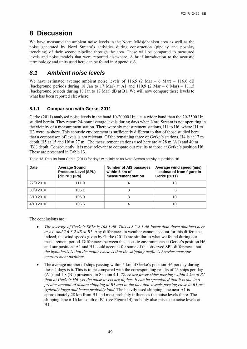
FOI-R--3469--SE

49

8 Discussion We have measured the ambient noise levels in the Norra Midsjöbanken area as well as the noise generated by Nord Stream’s activities during construction (pipelay and post-lay trenching) of their second pipeline through the area. These will be compared to measured levels and noise models that were reported elsewhere. A brief introduction to the acoustic terminology and units used here can be found in Appendix A.

8.1 Ambient noise levels We have estimated average ambient noise levels of 116.5 (2 Mar – 6 Mar) – 116.6 dB (background periods during 18 Jan to 17 Mar) at A1 and 110.9 (2 Mar – 6 Mar) – 111.5 (background periods during 18 Jan to 17 Mar) dB at B1. We will now compare these levels to what has been reported elsewhere.

8.1.1 Comparison with Gerke, 2011

Gerke (2011) analysed noise levels in the band 10-20000 Hz, i.e. a wider band than the 20-3500 Hz studied herein. They report 24-hour average levels during days when Nord Stream is not operating in the vicinity of a measurement station. There were six measurement stations, H1 to H6, where H1 to H3 were in-shore. This acoustic environment is sufficiently different to that of those studied here that a comparison of levels is not relevant. Of the remaining three of Gerke’s stations, H4 is at 17 m depth, H5 at 15 and H6 at 27 m. The measurement stations used here are at 28 m (A1) and 40 m (B1) depth. Consequently, it is most relevant to compare our results to those at Gerke’s position H6. These are presented in Table 13.

Table 13. Results from Gerke (2011) for days with little or no Nord Stream activity at position H6.

Date Average Sound Pressure Level (SPL) [dB re 1 µPa]

Number of AIS passages within 5 km of measurement station

Average wind speed (m/s) – estimated from figure in Gerke (2011)

27/9 2010 111.9 4 13

30/9 2010 105.1 8 6

3/10 2010 106.0 8 10

4/10 2010 106.6 4 10

The conclusions are:

The average of Gerke’s SPLs is 108.3 dB. This is 8.2-8.3 dB lower than those obtained here at A1, and 2.6-3.2 dB at B1. Any differences in weather cannot account for this difference; indeed, the wind speeds given by Gerke (2011) are similar to what we found during our measurement period. Differences between the acoustic environments at Gerke’s position H6 and our positions A1 and B1 could account for some of the observed SPL differences, but the hypothesis is that the major cause is that the shipping traffic is heavier near our measurement positions.

The average number of ships passing within 5 km of Gerke’s position H6 per day during these 4 days is 6. This is to be compared with the corresponding results of 23 ships per day (A1) and 1.8 (B1) presented in Section 4.1. There are fewer ships passing within 5 km of B1 than at Gerke’s H6, yet the noise levels are higher. It can be speculated that it is due to a greater amount of distant shipping at B1 and to the fact that vessels passing close to B1 are typically large and hence probably loud. The heavily used shipping lane near A1 is approximately 28 km from B1 and most probably influences the noise levels there. The shipping lane 6-16 km south of B1 (see Figure 14) probably also raises the noise levels at B1.

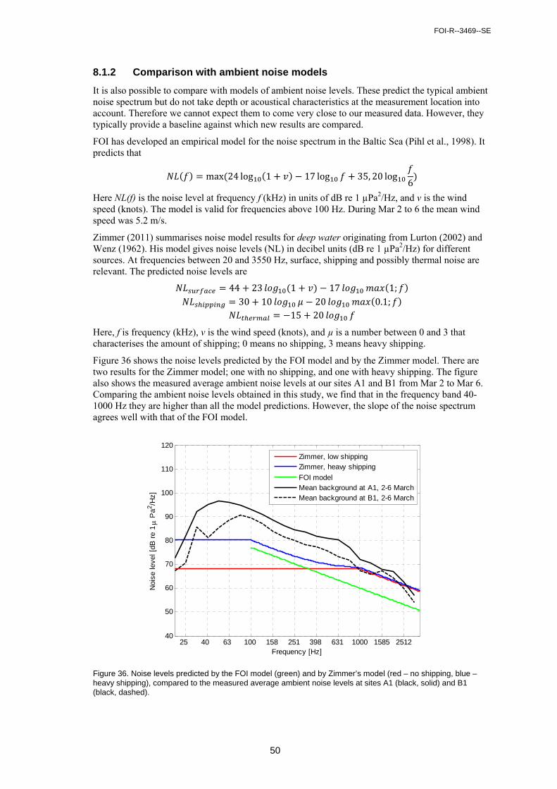
FOI-R--3469--SE

50

8.1.2 Comparison with ambient noise models

It is also possible to compare with models of ambient noise levels. These predict the typical ambient noise spectrum but do not take depth or acoustical characteristics at the measurement location into account. Therefore we cannot expect them to come very close to our measured data. However, they typically provide a baseline against which new results are compared.

FOI has developed an empirical model for the noise spectrum in the Baltic Sea (Pihl et al., 1998). It predicts that

max 24 log 1 17 log 35, 20 log6

Here NL(f) is the noise level at frequency f (kHz) in units of dB re 1 µPa2/Hz, and v is the wind speed (knots). The model is valid for frequencies above 100 Hz. During Mar 2 to 6 the mean wind speed was 5.2 m/s.

Zimmer (2011) summarises noise model results for deep water originating from Lurton (2002) and Wenz (1962). His model gives noise levels (NL) in decibel units (dB re 1 µPa2/Hz) for different sources. At frequencies between 20 and 3550 Hz, surface, shipping and possibly thermal noise are relevant. The predicted noise levels are

44 23 1 17 1;30 10 20 0.1;

15 20

Here, f is frequency (kHz), v is the wind speed (knots), and µ is a number between 0 and 3 that characterises the amount of shipping; 0 means no shipping, 3 means heavy shipping.

Figure 36 shows the noise levels predicted by the FOI model and by the Zimmer model. There are two results for the Zimmer model; one with no shipping, and one with heavy shipping. The figure also shows the measured average ambient noise levels at our sites A1 and B1 from Mar 2 to Mar 6. Comparing the ambient noise levels obtained in this study, we find that in the frequency band 40-1000 Hz they are higher than all the model predictions. However, the slope of the noise spectrum agrees well with that of the FOI model.

Figure 36. Noise levels predicted by the FOI model (green) and by Zimmer’s model (red – no shipping, blue – heavy shipping), compared to the measured average ambient noise levels at sites A1 (black, solid) and B1 (black, dashed).

25 40 63 100 158 251 398 631 1000 1585 251240

50

60

70

80

90

100

110

120

Frequency [Hz]

Noi

se le

vel [

dB r

e 1

Pa2 /H

z]

Zimmer, low shippingZimmer, heavy shipping

FOI modelMean background at A1, 2-6 MarchMean background at B1, 2-6 March

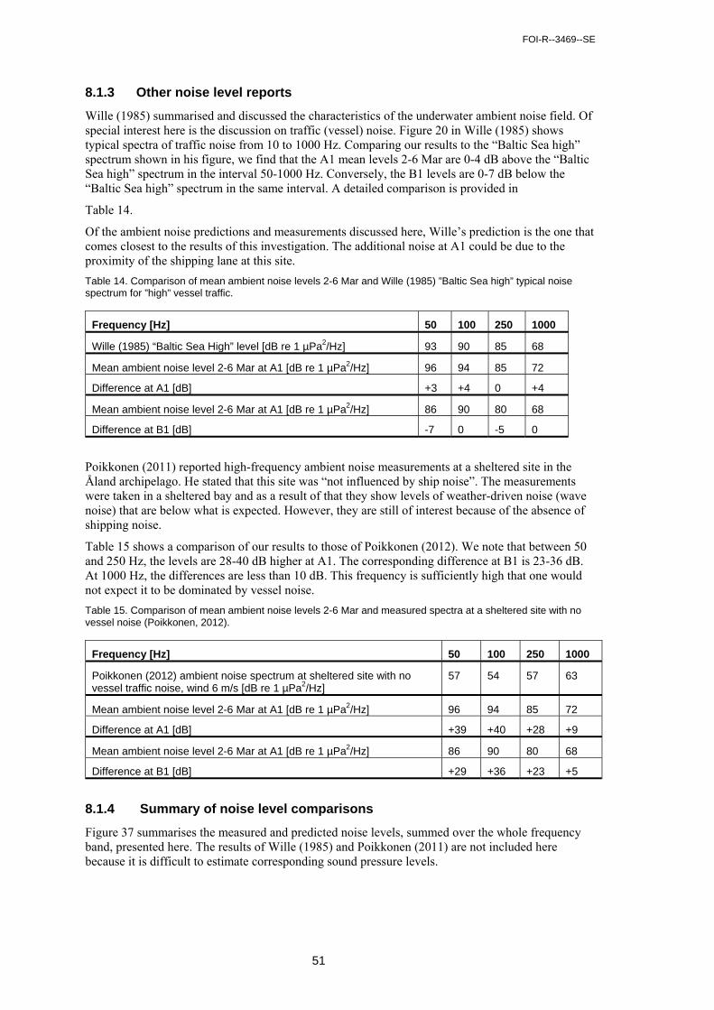
FOI-R--3469--SE

51

8.1.3 Other noise level reports

Wille (1985) summarised and discussed the characteristics of the underwater ambient noise field. Of special interest here is the discussion on traffic (vessel) noise. Figure 20 in Wille (1985) shows typical spectra of traffic noise from 10 to 1000 Hz. Comparing our results to the “Baltic Sea high” spectrum shown in his figure, we find that the A1 mean levels 2-6 Mar are 0-4 dB above the “Baltic Sea high” spectrum in the interval 50-1000 Hz. Conversely, the B1 levels are 0-7 dB below the “Baltic Sea high” spectrum in the same interval. A detailed comparison is provided in

Table 14.

Of the ambient noise predictions and measurements discussed here, Wille’s prediction is the one that comes closest to the results of this investigation. The additional noise at A1 could be due to the proximity of the shipping lane at this site.

Table 14. Comparison of mean ambient noise levels 2-6 Mar and Wille (1985) ”Baltic Sea high” typical noise spectrum for ”high” vessel traffic.

Frequency [Hz] 50 100 250 1000

Wille (1985) “Baltic Sea High” level [dB re 1 µPa2/Hz] 93 90 85 68

Mean ambient noise level 2-6 Mar at A1 [dB re 1 µPa2/Hz] 96 94 85 72

Difference at A1 [dB] +3 +4 0 +4

Mean ambient noise level 2-6 Mar at A1 [dB re 1 µPa2/Hz] 86 90 80 68

Difference at B1 [dB] -7 0 -5 0

Poikkonen (2011) reported high-frequency ambient noise measurements at a sheltered site in the Åland archipelago. He stated that this site was “not influenced by ship noise”. The measurements were taken in a sheltered bay and as a result of that they show levels of weather-driven noise (wave noise) that are below what is expected. However, they are still of interest because of the absence of shipping noise.

Table 15 shows a comparison of our results to those of Poikkonen (2012). We note that between 50 and 250 Hz, the levels are 28-40 dB higher at A1. The corresponding difference at B1 is 23-36 dB. At 1000 Hz, the differences are less than 10 dB. This frequency is sufficiently high that one would not expect it to be dominated by vessel noise.

Table 15. Comparison of mean ambient noise levels 2-6 Mar and measured spectra at a sheltered site with no vessel noise (Poikkonen, 2012).

Frequency [Hz] 50 100 250 1000

Poikkonen (2012) ambient noise spectrum at sheltered site with no vessel traffic noise, wind 6 m/s [dB re 1 µPa2/Hz]

57 54 57 63

Mean ambient noise level 2-6 Mar at A1 [dB re 1 µPa2/Hz] 96 94 85 72

Difference at A1 [dB] +39 +40 +28 +9

Mean ambient noise level 2-6 Mar at A1 [dB re 1 µPa2/Hz] 86 90 80 68

Difference at B1 [dB] +29 +36 +23 +5

8.1.4 Summary of noise level comparisons

Figure 37 summarises the measured and predicted noise levels, summed over the whole frequency band, presented here. The results of Wille (1985) and Poikkonen (2011) are not included here because it is difficult to estimate corresponding sound pressure levels.

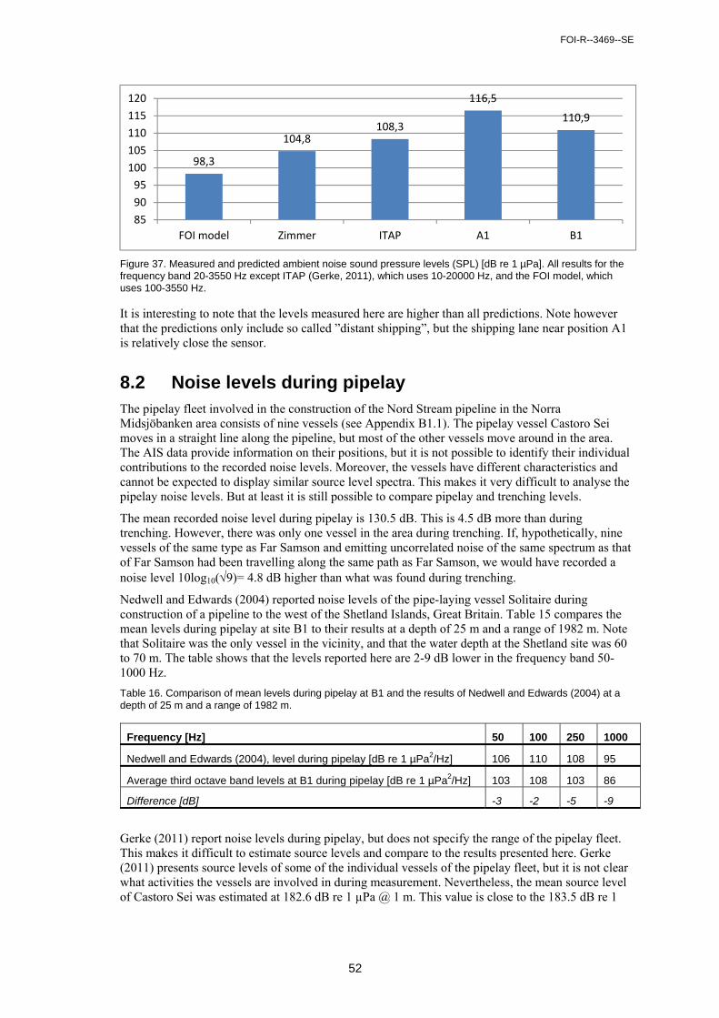
FOI-R--3469--SE

52

Figure 37. Measured and predicted ambient noise sound pressure levels (SPL) [dB re 1 µPa]. All results for the frequency band 20-3550 Hz except ITAP (Gerke, 2011), which uses 10-20000 Hz, and the FOI model, which uses 100-3550 Hz.

It is interesting to note that the levels measured here are higher than all predictions. Note however that the predictions only include so called ”distant shipping”, but the shipping lane near position A1 is relatively close the sensor.

8.2 Noise levels during pipelay The pipelay fleet involved in the construction of the Nord Stream pipeline in the Norra Midsjöbanken area consists of nine vessels (see Appendix B1.1). The pipelay vessel Castoro Sei moves in a straight line along the pipeline, but most of the other vessels move around in the area. The AIS data provide information on their positions, but it is not possible to identify their individual contributions to the recorded noise levels. Moreover, the vessels have different characteristics and cannot be expected to display similar source level spectra. This makes it very difficult to analyse the pipelay noise levels. But at least it is still possible to compare pipelay and trenching levels.

The mean recorded noise level during pipelay is 130.5 dB. This is 4.5 dB more than during trenching. However, there was only one vessel in the area during trenching. If, hypothetically, nine vessels of the same type as Far Samson and emitting uncorrelated noise of the same spectrum as that of Far Samson had been travelling along the same path as Far Samson, we would have recorded a noise level 10log10(9)= 4.8 dB higher than what was found during trenching.

Nedwell and Edwards (2004) reported noise levels of the pipe-laying vessel Solitaire during construction of a pipeline to the west of the Shetland Islands, Great Britain. Table 15 compares the mean levels during pipelay at site B1 to their results at a depth of 25 m and a range of 1982 m. Note that Solitaire was the only vessel in the vicinity, and that the water depth at the Shetland site was 60 to 70 m. The table shows that the levels reported here are 2-9 dB lower in the frequency band 50-1000 Hz.

Table 16. Comparison of mean levels during pipelay at B1 and the results of Nedwell and Edwards (2004) at a depth of 25 m and a range of 1982 m.

Frequency [Hz] 50 100 250 1000

Nedwell and Edwards (2004), level during pipelay [dB re 1 µPa2/Hz] 106 110 108 95

Average third octave band levels at B1 during pipelay [dB re 1 µPa2/Hz] 103 108 103 86

Difference [dB] -3 -2 -5 -9

Gerke (2011) report noise levels during pipelay, but does not specify the range of the pipelay fleet. This makes it difficult to estimate source levels and compare to the results presented here. Gerke (2011) presents source levels of some of the individual vessels of the pipelay fleet, but it is not clear what activities the vessels are involved in during measurement. Nevertheless, the mean source level of Castoro Sei was estimated at 182.6 dB re 1 µPa @ 1 m. This value is close to the 183.5 dB re 1

98,3

104,8108,3

116,5

110,9

85

90

95

100

105

110

115

120

FOI model Zimmer ITAP A1 B1

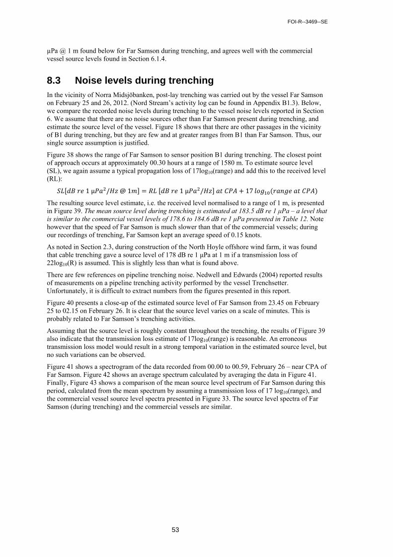
FOI-R--3469--SE

53

µPa @ 1 m found below for Far Samson during trenching, and agrees well with the commercial vessel source levels found in Section 6.1.4.

8.3 Noise levels during trenching In the vicinity of Norra Midsjöbanken, post-lay trenching was carried out by the vessel Far Samson on February 25 and 26, 2012. (Nord Stream’s activity log can be found in Appendix B1.3). Below, we compare the recorded noise levels during trenching to the vessel noise levels reported in Section 6. We assume that there are no noise sources other than Far Samson present during trenching, and estimate the source level of the vessel. Figure 18 shows that there are other passages in the vicinity of B1 during trenching, but they are few and at greater ranges from B1 than Far Samson. Thus, our single source assumption is justified.

Figure 38 shows the range of Far Samson to sensor position B1 during trenching. The closest point of approach occurs at approximately 00.30 hours at a range of 1580 m. To estimate source level (SL), we again assume a typical propagation loss of 17log10(range) and add this to the received level (RL):

1μ / @1 1μ / 17

The resulting source level estimate, i.e. the received level normalised to a range of 1 m, is presented in Figure 39. The mean source level during trenching is estimated at 183.5 dB re 1 μPa – a level that is similar to the commercial vessel levels of 178.6 to 184.6 dB re 1 μPa presented in Table 12. Note however that the speed of Far Samson is much slower than that of the commercial vessels; during our recordings of trenching, Far Samson kept an average speed of 0.15 knots.

As noted in Section 2.3, during construction of the North Hoyle offshore wind farm, it was found that cable trenching gave a source level of 178 dB re 1 μPa at 1 m if a transmission loss of 22log10(R) is assumed. This is slightly less than what is found above.

There are few references on pipeline trenching noise. Nedwell and Edwards (2004) reported results of measurements on a pipeline trenching activity performed by the vessel Trenchsetter. Unfortunately, it is difficult to extract numbers from the figures presented in this report.

Figure 40 presents a close-up of the estimated source level of Far Samson from 23.45 on February 25 to 02.15 on February 26. It is clear that the source level varies on a scale of minutes. This is probably related to Far Samson’s trenching activities.

Assuming that the source level is roughly constant throughout the trenching, the results of Figure 39 also indicate that the transmission loss estimate of 17log10(range) is reasonable. An erroneous transmission loss model would result in a strong temporal variation in the estimated source level, but no such variations can be observed.

Figure 41 shows a spectrogram of the data recorded from 00.00 to 00.59, February 26 – near CPA of Far Samson. Figure 42 shows an average spectrum calculated by averaging the data in Figure 41. Finally, Figure 43 shows a comparison of the mean source level spectrum of Far Samson during this period, calculated from the mean spectrum by assuming a transmission loss of 17 log10(range), and the commercial vessel source level spectra presented in Figure 33. The source level spectra of Far Samson (during trenching) and the commercial vessels are similar.

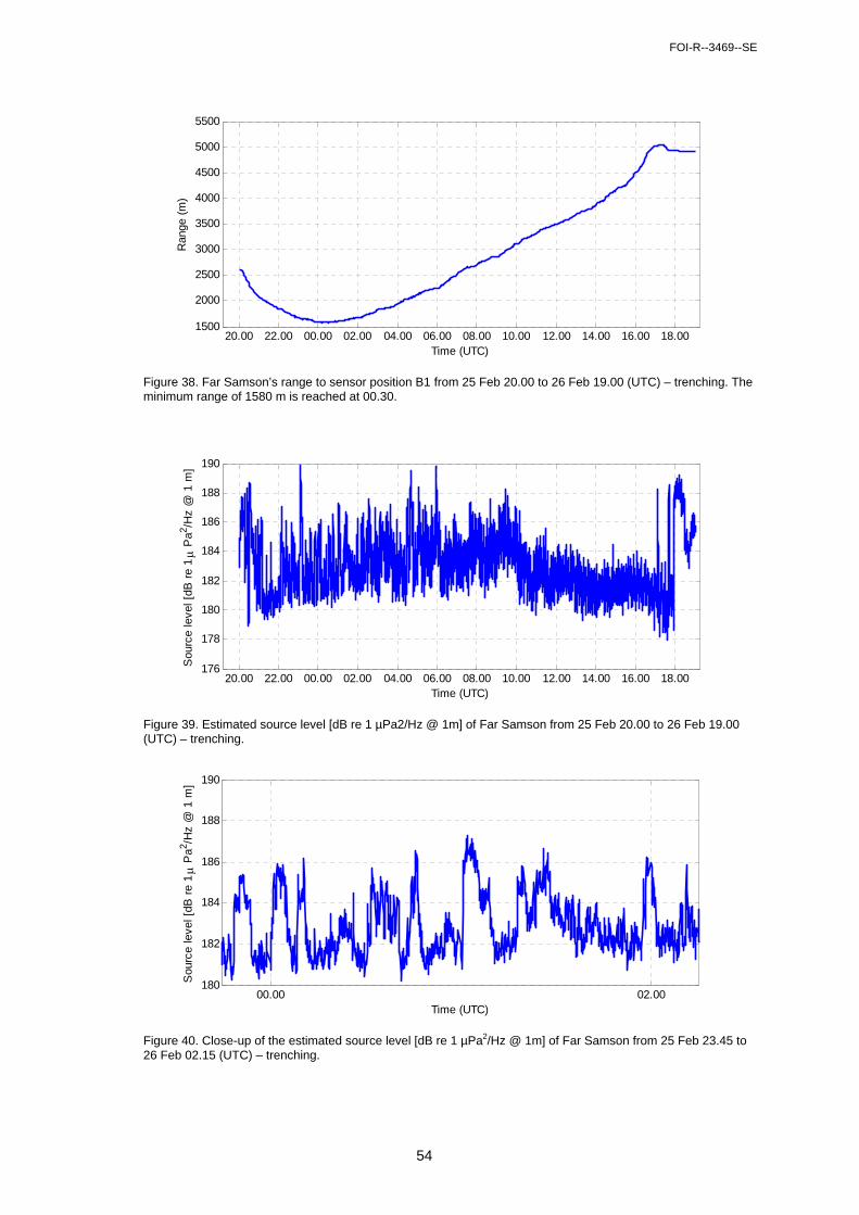
FOI-R--3469--SE

54

Figure 38. Far Samson’s range to sensor position B1 from 25 Feb 20.00 to 26 Feb 19.00 (UTC) – trenching. The minimum range of 1580 m is reached at 00.30.

Figure 39. Estimated source level [dB re 1 µPa2/Hz @ 1m] of Far Samson from 25 Feb 20.00 to 26 Feb 19.00 (UTC) – trenching.

Figure 40. Close-up of the estimated source level [dB re 1 µPa2/Hz @ 1m] of Far Samson from 25 Feb 23.45 to 26 Feb 02.15 (UTC) – trenching.

20.00 22.00 00.00 02.00 04.00 06.00 08.00 10.00 12.00 14.00 16.00 18.001500

2000

2500

3000

3500

4000

4500

5000

5500

Time (UTC)

Ran

ge (

m)

20.00 22.00 00.00 02.00 04.00 06.00 08.00 10.00 12.00 14.00 16.00 18.00176

178

180

182

184

186

188

190

Time (UTC)

Sou

rce

leve

l [dB

re

1

Pa2 /H

z @

1 m

]

00.00 02.00180

182

184

186

188

190

Time (UTC)

Sou

rce

leve

l [dB

re

1

Pa2 /H

z @

1 m

]

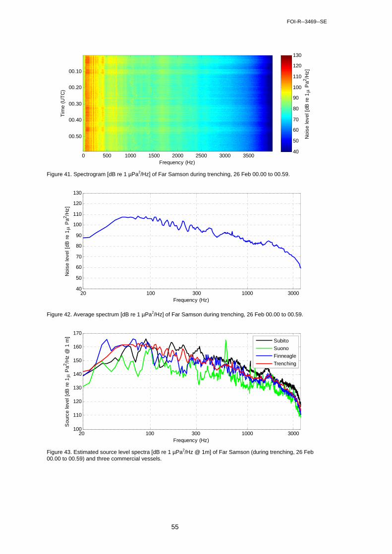
FOI-R--3469--SE

55

Figure 41. Spectrogram [dB re 1 µPa2/Hz] of Far Samson during trenching, 26 Feb 00.00 to 00.59.

Figure 42. Average spectrum [dB re 1 µPa2/Hz] of Far Samson during trenching, 26 Feb 00.00 to 00.59.

Figure 43. Estimated source level spectra [dB re 1 µPa2/Hz @ 1m] of Far Samson (during trenching, 26 Feb 00.00 to 00.59) and three commercial vessels.

Tim

e (U

TC

)

Frequency (Hz)

0 500 1000 1500 2000 2500 3000 3500

00.10

00.20

00.30

00.40

00.50 Noi

se le

vel [

dB r

e 1

Pa2 /H

z]

40

50

60

70

80

90

100

110

120

130

20 100 300 1000 300040

50

60

70

80

90

100

110

120

130

Frequency (Hz)

Noi

se le

vel [

dB r

e 1

Pa2 /H

z]

20 100 300 1000 3000100

110

120

130

140

150

160

170

Frequency (Hz)

Sou

rce

leve

l [dB

re

1

Pa2 /H

z @

1 m

]

Subito

Suono

Finneagle

Trenching

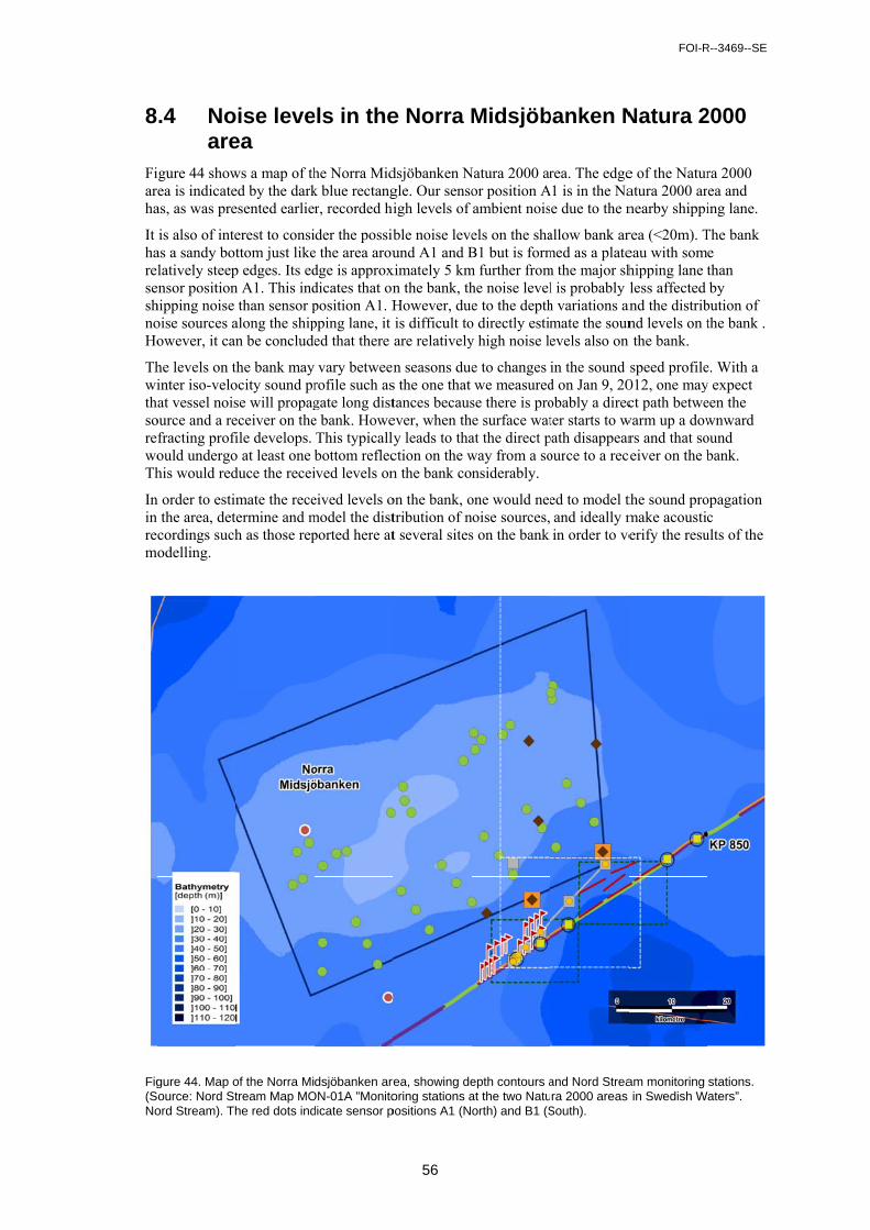
8

Fiarha

It hareseshnoHo

ThwithsorewoTh

Inin rem

Fig(SNo

.4 Noare

igure 44 showrea is indicateas, as was pre

is also of inteas a sandy botlatively steep

ensor positionhipping noise oise sources aowever, it can

he levels on tinter iso-veloat vessel nois

ource and a refracting profiould undergohis would red

n order to estim the area, detcordings suchodelling.

gure 44. Map oource: Nord Stord Stream). Th

oise leveea ws a map of thed by the darkesented earlie

erest to consittom just like

p edges. Its edn A1. This ind

than sensor palong the shipn be conclude

the bank may ocity sound prse will propageceiver on thefile develops. o at least one bduce the recei

mate the receermine and mh as those rep

of the Norra Mitream Map MOhe red dots ind

els in the

he Norra Midk blue rectangr, recorded hi

der the possibe the area aroudge is approxdicates that onposition A1. Hpping lane, it ed that there

vary betweenrofile such asgate long diste bank. HoweThis typicallybottom reflecived levels on

eived levels omodel the distported here at

dsjöbanken areON-01A ”Monitodicate sensor p

56

e Norra M

dsjöbanken Ngle. Our sensoigh levels of

ble noise leveund A1 and B

ximately 5 kmn the bank, thHowever, dueis difficult toare relatively

n seasons dues the one that tances becausever, when thy leads to thaction on the wn the bank co

on the bank, otribution of nt several sites

rea, showing deoring stations a

positions A1 (N

Midsjöb

Natura 2000 aror position Aambient nois

els on the shaB1 but is form

m further fromhe noise levele to the depth

o directly estimy high noise le

e to changes we measured

se there is proe surface wat

at the direct pway from a sonsiderably.

one would neenoise sources,s on the bank

epth contours aat the two Natuorth) and B1 (S

banken N

rea. The edgeA1 is in the Na

e due to the n

allow bank armed as a platem the major shl is probably lh variations anmate the sounevels also on

in the sound d on Jan 9, 20obably a directer starts to w

path disappearource to a rec

ed to model tand ideally min order to ve

and Nord Streara 2000 areas

South).

FOI-R

Natura 2

e of the Naturatura 2000 arnearby shippi

rea (<20m). Teau with somhipping lane tless affected

and the distribnd levels on t

n the bank.

speed profile012, one mayct path betwe

warm up a dowrs and that so

ceiver on the b

the sound promake acousticerify the resu

am monitoring in Swedish W

R--3469--SE

2000

ra 2000 ea and ing lane.

The bank e than by

bution of the bank .

e. With a y expect een the wnward ound bank.

opagation c

ults of the

stations. aters”.

FOI-R--3469--SE

57

9 Conclusions The aim of this study was to measure and quantify the noise during Nord Stream’s construction and trenching activities as well as the ambient noise including commercial shipping noise. We have presented noise levels at two locations, one close to a major shipping lane but far from the Nord Stream pipeline route, and the other close to the pipeline route. The recorded noise data was analysed at frequencies up to 3500 Hz. Third octave band spectra and sound pressure level evolutions as well as statistics were calculated for each of the hydrophones and during different conditions. Average ambient noise levels of 116.5-116.6 and 110.9-111.5 dB re 1 µPa were estimated at the two locations, the higher levels measured at the site that was closer to the shipping lane. Compared to previous results and predictions made by ambient noise models, we found that the noise levels at Norra Midsjöbanken are consistently higher. We speculated that this was due to the proximity of shipping lanes and the large numbers of passing ships.

The mean noise level estimated at the site closest to the pipeline during trenching was 126.0 dB re 1 µPa. The trenching was performed by the vessel Far Samson. The source level of this vessel during trenching was estimated to 183.5 dB re 1 µPa @ 1m using AIS information on its position. In a similar manner, we estimated the source levels of three commercial vessels and obtained results of 178.6 to 184.6 dB re 1 µPa @ 1m. We conclude that the source level of the vessel Far Samson during trenching is not greater than that of a commercial vessel.

The mean noise level estimated at the site closest to the pipeline during pipelay was 130.5 dB re 1 µPa. Compared to the noise level during trenching, the level during pipelay was 4.5 dB higher. We showed that this increase over the trenching level is consistent with an assumption that each of the nine vessels in the pipelay fleet displays a source level similar to those of the commercial vessels.

Finally, we concluded that the vessel traffic in the Norra Midsjöbanken area is so intense that, using omnidirectional sensors, it is difficult to measure a noise level undisturbed by shipping.

FOI-R--3469--SE

58

10 Implications and suggested future work In the vicinity of Norra Midsjöbanken, the construction and trenching of the second Nord Stream pipeline generated noise at a level and spectral distribution that was similar to that of one or more commercial ships. These acoustic disturbances were localised and temporary and hence also in that respect resembled the noise radiated by a commercial vessel. The noise levels during pipelay and trenching found here agreed with previously reported levels.

This study has found high levels of ambient noise at two measurement stations located in the Baltic Sea, approximately 50 km from nearest land. The noise was dominated by shipping noise from the nearby shipping lanes, and shipping was so intense that it was difficult to find a noise sample that was undisturbed by shipping. We compared our results to previous measurements from areas with less shipping. Gerke (2011) presented results from an acoustic environment similar to the one at our stations, but found levels 3-8 dB lower than those reported here. Poikkonen (2012) found power spectral densities 5-40 dB lower than those reported here in the frequency band 50-1000 Hz. These measurements were taken in a sheltered bay and the data were stated to be undisturbed by shipping. This indicates the magnitude of the influence of shipping noise on the Baltic Sea noise levels. This study analysed noise at frequencies up to 3500 Hz. In order to further quantify the noise levels in the Baltic Sea, it would be interesting to make additional recordings at higher frequencies.

The 5-6 dB difference in sound pressure level between the two measurement sites indicate that the distance to shipping lanes has a significant influence on the noise levels. A relevant future study would be to create a map of the noise levels around the shipping lane, quantifying the decay of noise level with distance from the shipping lane. This would permit one to judge both the scale and the severity of the noise pollution of the Baltic Sea soundscape caused by a shipping lane. The data presented in this report can be used in such a study, but would need to be complemented with measurements at more stations as well as sound propagation modelling. Using a directional hydrophone or an array of hydrophones would permit one to separate the noise caused by different vessels and to estimate an ambient noise level undisturbed by local shipping – a task that, due to the intensity of the vessel traffic, we could not fulfil in this study.

We did not directly measure noise levels on the biologically important shallow bank area of Norra Midsjöbanken, but based on the results presented here we argue that there are probably high levels of shipping noise on the bank. An interesting and relevant future endeavour would be to determine the noise levels on the bank by direct measurement and modelling of noise propagation in order to determine the relative contribution of noise from the different shipping lanes to the overall noise level. This could permit forecasts of how the noise levels were to change if shipping lanes were moved or vessel noise regulated.

This study has not suffered from losses of data due to technical failure or even loss of whole rigs to trawling or other interference. Although one cannot conclusively argue that this is entirely thanks to our efforts to avoid such losses, we stress that making good quality underwater acoustic measurements requires considerable care and knowledge of this discipline, and that it is important to pay attention to the choice of the measurement locations and the mechanical as well as electrical design of the measurement rigs.

Finally, perhaps the most important future endeavour is to assess how the ambient noise affects life at Norra Midsjöbanken, and, in a wider context, to learn more about the effects of noise in our seas and oceans on the marine environment. Fish, marine mammals and other organisms use sound for communication, navigation and for finding food. High noise levels can make all these things difficult as well as, in severe cases, cause temporary or permanent hearing loss. Noise can therefore have a negative impact even on a population level. This may be crucial for threatened species.

FOI-R--3469--SE

59

Acknowledgements The funding for this study was provided by Nord Stream and Naturvårdsverket (Swedish Environment Protection Agency). Data was provided by the Swedish Maritime Authority (AIS), the Swedish Agency for Marine and Water Management (VMS), and Försvarsmaktens Meteorologiska och Oceanografiska Centrum METOCC (Weather). We thank Patrik Jonsson for assistance with the VMS data and the staff of the fishing vessel Kingston for their helpful attitude and strong arms. Finally we acknowledge the contribution of our FOI colleagues Leif Persson, Peter Sigray, Stefan Petrovic, Malin Lennartsson, Niels Jacobsen, Markus Linné, Lisa Rosenqvist, and Torbjörn Ståhlsten.

FOI-R--3469--SE

60

References Ainslie, M. A., de Jong, C. A. F., Doi, H. S., Blacquière, G., Marasini, C. 2009. Assessment of natural and anthropogenic sound sources and acoustic propagation in the North Sea. TNO report, TNO-DV 2009 C085, Haag, Nederländerna. 110 pp. (www.noordzeeloket.nl)

Andersson, M., Sigray, P., Persson, L., 2011. Ljud från vindkraftverk i havet och dess påverkan på fisk. Vindval Rapport 6436 (in Swedish). Swedish Environment Protection Agency (Naturvårdsverket). 41 pp. (http://www.naturvardsverket.se/Documents/publikationer6400/978-91-620-6436-5.pdf)

Andrew, R. K., Howe, B. M., Mercer, J. A., 2002. Ocean ambient sound: Comparing the 1960s with the 1990s for a receiver off the California coast. Acoustic Research Letters Online 3 (2), pp. 65–70.

Arveson, P.T., Vendittis, D.J., 2000. Radiated noise characteristics of a modern cargo ship. Journal of the Acoustical Society of America 107 (1), pp. 118–129.

European Union, 2008. Directive 2008/56/EC of the European Parliament and of the Council of 17 June 2008 establishing a framework for community action in the field of marine environmental policy (Marine Strategy Framework Directive).

Gerke, P. 2011. The Nord Stream Monitoring - Measurement of the hydro-sound pollution. Institut für technische und angewandte Physik GmbH (ITAP). Nord Stream report G-PE-LFG-MON-500-UNWNOISE-A. 158 pp.

Hatch, L., Clark, C., Merrick, R.,Van Parijs, S., Ponirakis, D., Schwehr, C.,Thompson, M., Wiley, D., 2008. Characterizing the Relative Contributions of Large Vessels to Total Ocean Noise Fields: A Case Study Using the Gerry E. Studds Stellwagen Bank National Marine Sanctuary. Environmental Management 42 (5), pp. 735–752.

HELCOM, 2010. Atlas of the Baltic Sea. Helsinki Commission, Helsinki, Finland, 2010.

Hildebrand, J., 2009. Anthropogenic and natural sources of ambient noise in the ocean. Marine Ecology Progress Series 395, pp. 5-20.

IMO, 1974. Conversion for Safety of Life at Sea (SOLAS), Chapter V Safety and Navigation, Regulation 19 (amended Dec 2000). (http://www.imo.org/about/conventions/listofconventions/pages/international-convention-for-the-safety-of-life-at-sea-(solas),-1974.aspx)

Nedwell, J.R., Edwards, B,. 2004. A review of measurements of underwater man-made noise carried out by Subacoustech Ltd, 1993 – 2003. Subacoustech Report No: 534R0109. 136 pp. (http://www.subacoustech.com/information/downloads/reports/534R0109.pdf)

Nedwell, J., Langworthy, J., Howell, D., 2003. Assessment of sub-sea acoustic noise and vibration from offshore wind turbines and its impact on marine wildlife; initial measurements of underwater noise during construction of offshore windfarms, and comparison with background noise. Subacoustech Report No. 544 R 0424. 72 pp. (http://www.subacoustech.com/information/publications.shtml)

McDonald, M.A., Hildebrand, J.A., Wiggins, S.M., 2006. Increases in deep ocean ambient noise in the Northeast Pacific west of San Nicolas island, California. Journal of the Acoustical Society of America 120 (2), pp. 711-718.

Merchant, N.D., Witt, M.J., Blondel, P., Godley, B.J. and Smith, G.H., 2012. Assessing sound exposure from shipping in coastal waters using a single hydrophone and Automatic Identification System (AIS) data. Marine Pollution Bulletin 64 (7), pp.1320–1329.

Lurton, X., 2002. An Introduction to Underwater Acoustics. Springer Verlag, London. 680 pp.

OSPAR, 2009. Overview of the impacts of anthropogenic underwater sound in the marine environment, OSPAR Convention for the Protection of the Marine Environment of the North-East Atlantic. Biodiversity and Ecosystems Series, Publication Number 441/2009, 134 pp. (http://www.ospar.org/documents/dbase/publications/p00441_noise%20background%20document.pdf)

FOI-R--3469--SE

61

Pihl, J., Ivansson, S., Karlsson, P., Lennartsson, R., Levonen, M., Morén, P., Nilsson, B., Olsson, M., Staaf, Ö., Sundin, G., Söderberg, P., 1998. Underwater Acoustics in the Baltic. FOI report FOA-R--98-00727-409. Stockholm, Sweden.

Poikkonen, A., 2012. Measurements, analysis, and modeling of wind-driven ambient noise in shallow brackish water. Thesis for the degree of Doctor of Science in Technology, School of Electrical Engineering, Aalto University, Finland.

Popper, A.N., Hastings, M.C., 2009. The effect of anthropogenic sources of sound on fishes. Journal of Fish Biology 75, pp. 455-489.

Slabbekoorn, H., Bouton, N., van Opzeeland, I., Coers, A., ten Cate, C., Popper, A.N., 2010. “A noisy spring: the impact of globally rising underwater sound levels on fish. Trends in Ecology and Evolution 25 (7), pp. 419-427.

Southall, B.L., Bowles, A.E., Ellison, W.T., Finneran, J.J., Gentry, R.L., Greene, C.R. Jr., Kastak, D., Ketten, D.R., Miller, J.H., Nachtigall, P.E., Richardson, W.J., Thomas, J.A., and Tyack, P.L., 2007. Marine mammal noise exposure criteria: Initial scientific recommendations. Aquatic Mammals 33, pp. 411 – 521.

Ross, D., 1993. On ocean underwater ambient noise. Acoustic Bulletin 18, pp. 5–8.

Van der Graaf, A.J., Ainslie, M.A., André, M., Brensing, K., Dalen, J., Dekeling, R.P.A., Robinson, S., Tasker, M.L., Thomsen, F., Werner, S., 2012. European Marine Strategy Framework Directive - Good Environmental Status (MSFD GES): Report of the Technical Subgroup on Underwater noise and other forms of energy. 75 pp. (http://www.lab.upc.edu/papers/MSFD_Final_report_of_the_TSG_Noise_feb2012.pdf)

Wenz, G.M., 1962. Noise in the ocean: spectra and sources. Journal of the Acoustical Society of America 34, pp. 1936–1956.

Wille, P.C., 1985. Ambient Noise: Characteristics of the Noise Field. In H. G. Urban (ed.), Adaptive Methods in Underwater Acoustics, pp 13-36. D. Riedel Publishing Company. 740 pp.

Zimmer, W.M., 2011. Passive acoustic monitoring of cetaceans. Cambridge University Press. 356 pp.

FOI-R--3469--SE

62

Appendix A. Acoustic terminology

Sound Pressure Level (SPL)

A sound is a pressure fluctuation, and its amplitude is measured in pressure units (Pa or, more commonly, µPa). The amplitude of a sound is normally expressed using a logarithmic scale and is then called ”Sound Pressure Level” (SPL). The sound pressure value p is compared to a reference value pref. In water, the reference value is 1 µPa. The unit of SPL is decibel (dB) relative to the reference value. This is written ”dB re 1 µPa”. The sound pressure level is calculated as 20log10p/pref.If p = 100 µPa, p/pref = 100 and SPL = 40 dB re 1 µPa.

Power Spectral Density (PSD)

It is often of interest to calculate a sound’s power at different frequencies. One then calculates a (frequency) spectrum, which shows the sound’s power as a function of frequency. The spectrum of noise-like sounds is typically expressed as ”power per unit frequency” on a logarithmic scale. This is called a ”Power Spectral Density” (PSD). The unit of the PSD is dB re 1 uPa2/Hz.

Source Level (SL)

The source level of a sound source is the sound pressure that we would measure if we were at a distance of 1 m from the source. Source levels are useful for comparing different sources. Source levels are expressed in units of dB re 1 μPa @ 1m.

Received Level (RL)

The measured sound pressure level at the sensor.

Transmission loss (TL)

Transmission loss is the decay of a sound’s amplitude as it is transmitted through a medium. In water, if we measure far enough from the source, the transmission loss is often modelled as

log .

Here, the first term models geometrical spreading and the second absorption. M is a number between 10 and 20. In this report, the absorption term is ignored because we measure at relatively short distances, low frequencies, and in a sea of low salinity. The transmission loss can be used to estimate the source level from the received level:

SL = RL + TL.

Third octave band

An octave band is a band of frequencies whose upper edge frequency is twice its lower edge frequency. There are standard octave band edge and centre frequencies that simplify comparison of noise levels. When a higher frequency resolution than permitted by an octave band analysis is desired, one can employ third octave bands. As the name suggests, there are three third octave bands per octave band. Their edge frequencies follow a logarithmic pattern.

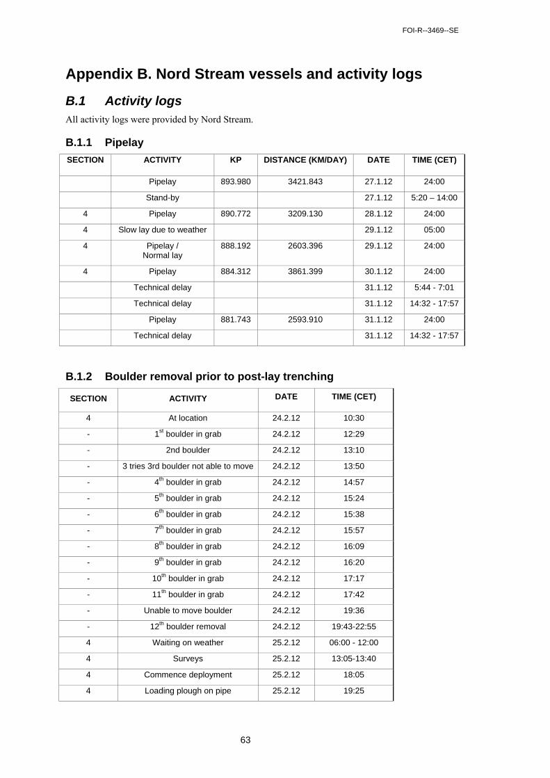
FOI-R--3469--SE

63

Appendix B. Nord Stream vessels and activity logs

B.1 Activity logs All activity logs were provided by Nord Stream.

B.1.1 Pipelay

SECTION ACTIVITY KP DISTANCE (KM/DAY) DATE TIME (CET)

Pipelay 893.980 3421.843 27.1.12 24:00

Stand-by 27.1.12 5:20 – 14:00

4 Pipelay 890.772 3209.130 28.1.12 24:00

4 Slow lay due to weather 29.1.12 05:00

4 Pipelay / Normal lay

888.192 2603.396 29.1.12 24:00

4 Pipelay 884.312 3861.399 30.1.12 24:00

Technical delay 31.1.12 5:44 - 7:01

Technical delay 31.1.12 14:32 - 17:57

Pipelay 881.743 2593.910 31.1.12 24:00

Technical delay 31.1.12 14:32 - 17:57

B.1.2 Boulder removal prior to post-lay trenching

SECTION ACTIVITY DATE TIME (CET)

4 At location 24.2.12 10:30

- 1st boulder in grab 24.2.12 12:29

- 2nd boulder 24.2.12 13:10

- 3 tries 3rd boulder not able to move 24.2.12 13:50

- 4th boulder in grab 24.2.12 14:57

- 5th boulder in grab 24.2.12 15:24

- 6th boulder in grab 24.2.12 15:38

- 7th boulder in grab 24.2.12 15:57

- 8th boulder in grab 24.2.12 16:09

- 9th boulder in grab 24.2.12 16:20

- 10th boulder in grab 24.2.12 17:17

- 11th boulder in grab 24.2.12 17:42

- Unable to move boulder 24.2.12 19:36

- 12th boulder removal 24.2.12 19:43-22:55

4 Waiting on weather 25.2.12 06:00 - 12:00

4 Surveys 25.2.12 13:05-13:40

4 Commence deployment 25.2.12 18:05

4 Loading plough on pipe 25.2.12 19:25

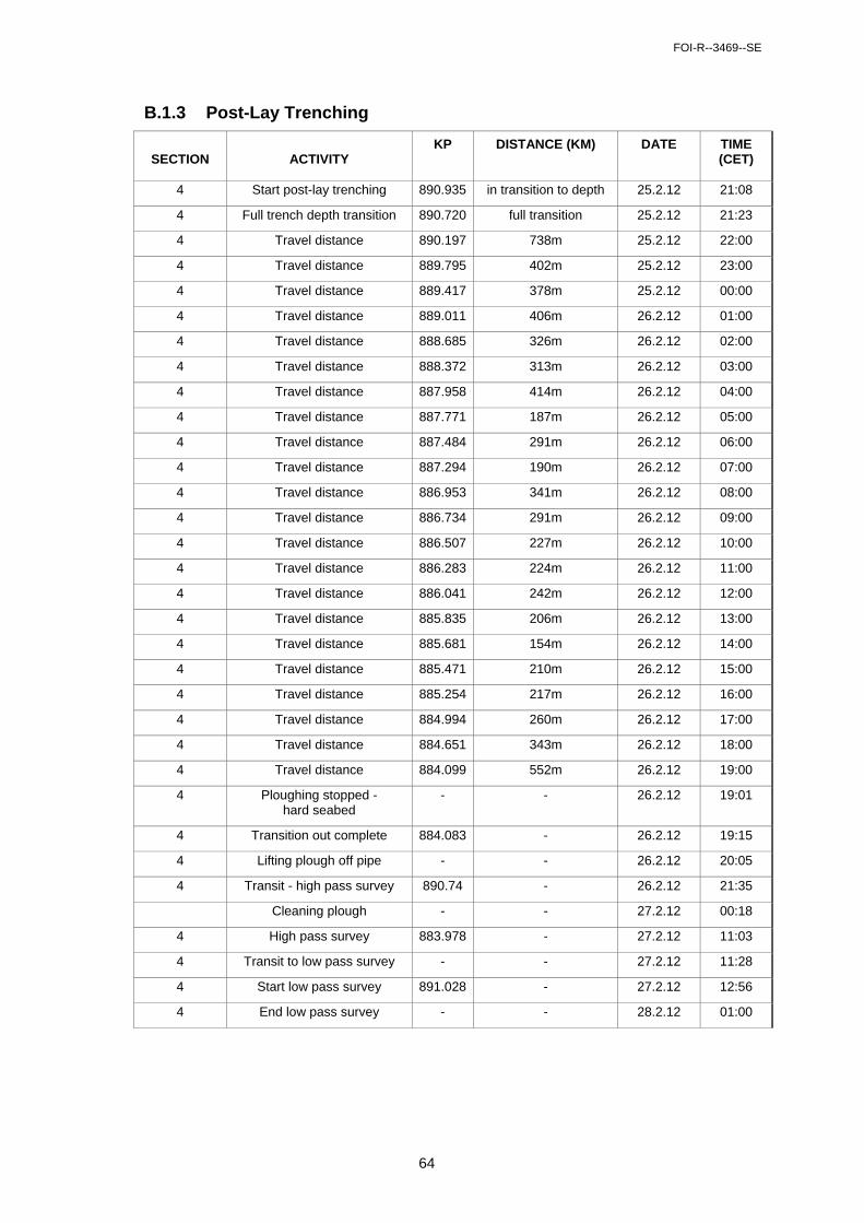
FOI-R--3469--SE

64

B.1.3 Post-Lay Trenching

SECTION ACTIVITY KP DISTANCE (KM) DATE TIME

(CET)

4 Start post-lay trenching 890.935 in transition to depth 25.2.12 21:08

4 Full trench depth transition 890.720 full transition 25.2.12 21:23

4 Travel distance 890.197 738m 25.2.12 22:00

4 Travel distance 889.795 402m 25.2.12 23:00

4 Travel distance 889.417 378m 25.2.12 00:00

4 Travel distance 889.011 406m 26.2.12 01:00

4 Travel distance 888.685 326m 26.2.12 02:00

4 Travel distance 888.372 313m 26.2.12 03:00

4 Travel distance 887.958 414m 26.2.12 04:00

4 Travel distance 887.771 187m 26.2.12 05:00

4 Travel distance 887.484 291m 26.2.12 06:00

4 Travel distance 887.294 190m 26.2.12 07:00

4 Travel distance 886.953 341m 26.2.12 08:00

4 Travel distance 886.734 291m 26.2.12 09:00

4 Travel distance 886.507 227m 26.2.12 10:00

4 Travel distance 886.283 224m 26.2.12 11:00

4 Travel distance 886.041 242m 26.2.12 12:00

4 Travel distance 885.835 206m 26.2.12 13:00

4 Travel distance 885.681 154m 26.2.12 14:00

4 Travel distance 885.471 210m 26.2.12 15:00

4 Travel distance 885.254 217m 26.2.12 16:00

4 Travel distance 884.994 260m 26.2.12 17:00

4 Travel distance 884.651 343m 26.2.12 18:00

4 Travel distance 884.099 552m 26.2.12 19:00

4 Ploughing stopped - hard seabed

- - 26.2.12 19:01

4 Transition out complete 884.083 - 26.2.12 19:15

4 Lifting plough off pipe - - 26.2.12 20:05

4 Transit - high pass survey 890.74 - 26.2.12 21:35

Cleaning plough - - 27.2.12 00:18

4 High pass survey 883.978 - 27.2.12 11:03

4 Transit to low pass survey - - 27.2.12 11:28

4 Start low pass survey 891.028 - 27.2.12 12:56

4 End low pass survey - - 28.2.12 01:00

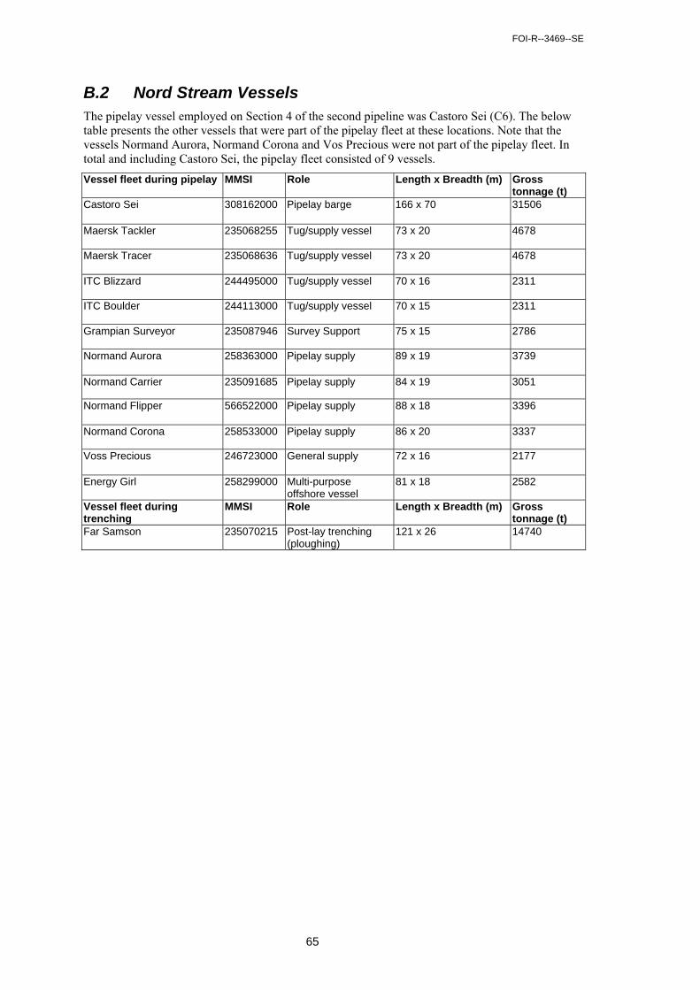
FOI-R--3469--SE

65

B.2 Nord Stream Vessels The pipelay vessel employed on Section 4 of the second pipeline was Castoro Sei (C6). The below table presents the other vessels that were part of the pipelay fleet at these locations. Note that the vessels Normand Aurora, Normand Corona and Vos Precious were not part of the pipelay fleet. In total and including Castoro Sei, the pipelay fleet consisted of 9 vessels.

Vessel fleet during pipelay MMSI Role Length x Breadth (m) Gross tonnage (t)

Castoro Sei 308162000 Pipelay barge 166 x 70 31506

Maersk Tackler 235068255 Tug/supply vessel 73 x 20 4678

Maersk Tracer 235068636 Tug/supply vessel 73 x 20 4678

ITC Blizzard 244495000 Tug/supply vessel 70 x 16 2311

ITC Boulder 244113000 Tug/supply vessel 70 x 15 2311

Grampian Surveyor 235087946 Survey Support 75 x 15 2786

Normand Aurora 258363000 Pipelay supply 89 x 19 3739

Normand Carrier 235091685 Pipelay supply 84 x 19 3051

Normand Flipper 566522000 Pipelay supply 88 x 18 3396

Normand Corona 258533000 Pipelay supply 86 x 20 3337

Voss Precious 246723000 General supply 72 x 16 2177

Energy Girl 258299000 Multi-purpose offshore vessel

81 x 18 2582

Vessel fleet during trenching

MMSI Role Length x Breadth (m) Gross tonnage (t)

Far Samson 235070215 Post-lay trenching (ploughing)

121 x 26 14740