Crust and uppermost mantle beneath the North China Craton, northeastern China, and the Sea of Japan...

Crust and uppermost mantle beneath the North China Craton,northeastern China, and the Sea of Japan from ambient noisetomography

Yong Zheng,1 Weisen Shen,2 Longquan Zhou,3 Yingjie Yang,1,4 Zujun Xie,1

and Michael H. Ritzwoller2

Received 28 June 2011; revised 30 October 2011; accepted 2 November 2011; published 21 December 2011.

[1] A 3‐D shear velocity model of the crust and uppermost mantle to a depth of 100 kmis presented beneath the North China Craton (NCC), northeastern China, the KoreanPeninsula, and the Sea of Japan. Ambient noise Rayleighwave tomography is applied to datafrom more than 300 broadband seismic stations from Chinese provincial networks(CEArray), the Japanese F‐Net, and the IRIS Global Seismic Network. Continuous datafrom 2007 to 2009 are used to produce group and phase velocity maps from 8 s to 45 speriods. The model is motivated to constrain the distributed intraplate volcanism, crustalextension, cratonic rejuvenation, and lithospheric thinning that are hypothesized forthe study region. Numerous robust features are observed that impose new constraints on thegeometry of these processes, but discussion concentrates only on four. (1) The North‐SouthGravity Lineament follows the ∼40 km contour in crustal thickness, and crustal thicknessis anticorrelated with water depth beneath the Sea of Japan, consistent with crustal isostasyfor a crust with laterally variable composition. (2) The lithosphere is thin (∼70 km) beneaththe Songliao‐Bohai Graben but seismically fast. (3) Even thinner more attenuatedlithosphere bounds three sides of the eastern NCC (in a horseshoe shape), identifying aregion of particularly intense tectonothermal modification where lithospheric rejuvenationmay have reached nearly to the base of the crust. (4) Low‐velocity anomalies reach upward(in a Y shape) in the mantle beneath the eastern and western borders of the Sea of Japan,extending well into continental East Asia in the west, and are separated by a ∼60 kmthick lithosphere beneath the central Sea of Japan. This anomaly may reflect relativelyshallow slab dehydration in the east and in the west may reflect deeper dehydration andconvective circulation in the mantle wedge overlying the stagnant slab.

Citation: Zheng, Y., W. Shen, L. Zhou, Y. Yang, Z. Xie, and M. H. Ritzwoller (2011), Crust and uppermost mantle beneath theNorth China Craton, northeastern China, and the Sea of Japan from ambient noise tomography, J. Geophys. Res., 116, B12312,doi:10.1029/2011JB008637.

1. Introduction

[2] The goal of this study and companion papers by Yanget al. [2010], Y. Yang et al. (A synoptic view of the dis-tribution and connectivity of the mid‐crustal low velocityzone beneath Tibet, submitted to Journal of GeophysicalResearch, 2011), Zheng et al. [2010b], and L. Zhou et al.(Ambient noise surface wave tomography of South China,submitted to Geophysical Journal International, 2011) is toadvance toward an integrated, highly resolved shear velocity

(Vs) model of the crust and uppermost mantle beneath China.Zhou et al. (submitted manuscript, 2011) focus on SoutheastChina, and Yang et al. [2010], Yang et al. (submitted man-uscript, 2011), and Zheng et al. [2010b] focus on westernChina and Tibet. The complementary focus of the currentpaper is the Sino‐Korean Craton, northeastern China, theKorean Peninsula, and the Sea of Japan. More than320 seismic stations from Chinese provincial networks innortheastern China and surrounding areas, Japanese F‐Netstations [Okada et al., 2004], and IRIS GSN stations are thebasis for this study (Figure 1). The resulting station and pathcoverage that emerges is unprecedented in this region. Inorder to place strong constraints on crustal structure, ambientnoise tomography is employed. As described below, ambientnoise tomography has already been applied in other regions ofChina (e.g., Tibet), at larger scales (e.g., across all of China)at a lower resolution, or in a part of the study region (e.g.,North China Platform, Korean peninsula), but a resultingintegrated, high‐resolution model of the crust and uppermostmantle of the entire region of study has never before been

1State Key Laboratory of Geodesy and Earth’s Dynamics, Institute ofGeodesy and Geophysics, Chinese Academy of Sciences, Wuhan, China.

2Center for Imaging the Earth’s Interior, Department of Physics,University of Colorado at Boulder, Boulder, Colorado, USA.

3China Earthquake Network Center, Beijing, China.4Australian Research Council Centre of Excellence for Core to Crust

Fluid Systems/GEMOC, Department of Earth and Planetary Sciences,Macquarie University, North Ryde, New South Wales, Australia.

Copyright 2011 by the American Geophysical Union.0148‐0227/11/2011JB008637

JOURNAL OF GEOPHYSICAL RESEARCH, VOL. 116, B12312, doi:10.1029/2011JB008637, 2011

B12312 1 of 25

http://dx.doi.org/10.1029/2011JB008637

constructed. Such a model is desired to illuminate a set ofinterconnected tectonic problems that make the Sino‐KoreanCraton, northeastern China, and the Sea of Japan a particu-larly fertile area for seismic tomography.[3] Northeastern China is composed of a mosaic of tectonic

blocks and lineated orogenic belts (Figure 2) that have beenarranged and modified by a long, complex, and in some casesenigmatic history of subduction, accretion, and collisiondating back to the Archean [e.g., Sengor and Natal’in, 1996;Yin and Nie, 1996; Yin, 2010]. In the south, the Sino‐KoreanCraton (SKC), delineated by solid red lines in Figure 2,is separated from the Yangtze Craton to the south by theQinling‐Dabie‐Sulu orogenic belt [Yin and Nie, 1993]. TheSKC itself consists of the Ordos Block, the North ChinaPlatform, Bohai Bay, the Korean Peninsula, as well as mar-ginal and intruding mountain ranges. The Chinese part of theSKC is usually referred to as the North China Craton (NCC)and is divided here into western, central, and eastern partsdelineated by dashed red lines. North of the SKC, theXing’an–East Mongolia block is separated from theSongliao‐Bohai graben by the North‐South Gravity Linea-ment (NSGL). The NSGL extends southward into the SKCnear the boundary between the central and eastern parts of theNorth China Craton. The Songliao‐Bohai graben, stretchingfrom the Songliao Basin to the Bohai Gulf, is flanked to theeast by the Tancheng‐Lujiang (Tanlu) Fault that extends intothe SKC and forms the eastern boundary of the North ChinaCraton. The Tanlu Fault also defines the western border of theNortheast Asia Fold Belt [e.g., Sengor and Natal’in, 1996;Yin and Nie, 1996].[4] Much of northeastern China has undergone extensive

tectonism during the late Mesozoic and Cenozoic eras [e.g.,Yin, 2010]. Northeastern China, bounded by the SKC to thesouth and the Sea of Japan back‐arc basin to the east, is partof eastern China’s Cenozoic volcanic zone [e.g., Ren et al.,2002]. Episodic volcanism has been particularly prom-inent along three volcanic mountain chains: Great Xing’anRange (GXAR), Lesser Xing’an Range (LXAR), Changbai

Mountains (CBM). Rifting and extension are believed to havebegun in the late Mesozoic [Tian et al., 1992] and have led tothe development of the Songliao Basin, although the Songliaobasement is traced back to the Archean [Rogers and Santosh,2006]. It has also been hypothesized that there is a physicallinkage between the sequential openings of the Songliaograben [e.g., Liu et al., 2001] and the Sea of Japan [Tatsumiet al., 1989; Jolivet et al., 1994]. The SKC formed largelyin the Archean, but it is a paradigm of an Archean craton thathas lost its lithospheric keel. Petrological and geochemicalevidence [e.g., Menzies et al., 1993; Griffin et al., 1998]suggests that typical cratonic lithosphere existed beneaththe entire SKC until at least the Ordovician, after which theSKC was reactivated and lithospheric thinning occurred atthe minimum beneath the eastern part of the NCC.[5] The physical mechanisms that have produced the

highly distributed volcanism, crustal extension, cratonicrejuvenation and lithospheric thinning that have occurredacross parts of northeastern China remain poorly under-stood [e.g., Deng et al., 2007; Chen, 2010]. These issuescan be illuminated with seismic images of velocity hetero-geneities, internal discontinuities, and crustal and mantleanisotropy, yet the vast majority of the studies to date havebeen geochemical or petrological in nature. Increasingly,

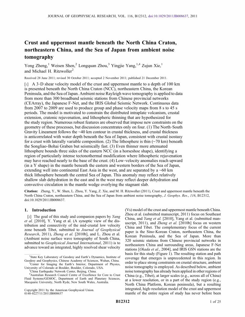
Figure 1. The broadband seismic stations used in this study.The blue triangles are the Chinese provincial broadbandseismic stations (CEArray), the red triangles are the F‐Netlong‐period stations, and the red squares are other broadbandstations, mostly from the IRIS GSN. The black box definesthe study region.

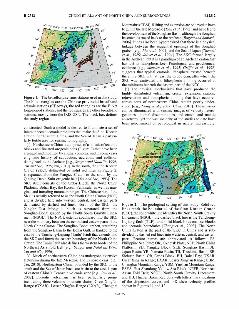
Figure 2. The geological setting of this study. Solid redlines mark the boundaries of the Sino‐Korean Craton(SKC), the solid white line identifies the North‐South GravityLineament (NSGL), the dashed black line is the Tancheng‐Lujiang fault (TLF), and solid black lines outline blocksand tectonic boundaries [Zhang et al., 2003]. The NorthChina Craton is the part of the SKC in China and is sub-divided by dashed red lines into western, central, and easternparts. Feature names are abbreviated as follows: PS,Philippine Sea Plate; OK, Okhotsk Plate; NCP, North ChinaPlatform; YB, Yangtze Block; SLB, Songliao Basin; JB,Japan Basin; YB, Yamato Basin; TB, Tsushima Basin; SB,Sichuan Basin; OR, Ordos Block; BH, Bohai Bay; GXAR,Great Xing’an Range; LXAR, Lesser Xing’an Range; CBM,Changbai Mountain Range; YSM, YinshanMountain Range;ESYS, East Shandong Yellow Sea Block; NEFB, NortheastAsian Fold Belt; NSGL, North‐South Gravity Lineament;and HB, Huabei Basin. Red dots with letters mark locationsof the dispersion curves and 1‐D shear velocity profilesshown in Figures 11 and 12.

ZHENG ET AL.: ANT OF NORTH CHINA AND SURROUNDINGS B12312B12312

2 of 25

seismological studies are adding new information due in partto the rapid expansion of seismic instrumentation in Chinaover the past few years [e.g., Zheng et al., 2010a]. Thesestudies include body wave tomography of the mantle [e.g.,Lebedev and Nolet, 2003; Huang and Zhao, 2006; Zhao,2009; Tian et al., 2009; Xu and Zhao, 2009; Li and van derHilst, 2010; Santosh et al., 2010] and of the crust [e.g., Sunand Toksöz, 2006]. Pn tomography [Li et al., 2011],receiver functions analyses [Zheng et al., 2006; Chen et al.,2009], and shear wave splitting studies have also been per-formed [Zhao et al., 2008; Bai et al., 2010; Li and Niu, 2010].Recent body wave results have focused mainly on the easternpart of the NCC, including efforts to image its thin intactlithosphere as well as the potential remnants of the delami-nated lithosphere near 400 km depth [e.g., Chen et al., 2009;Xu and Zhao, 2009].[6] At least parts of northeast China have been imaged

by larger‐scale teleseismic surface wave dispersion studies[e.g., Ritzwoller and Levshin, 1998; Ritzwoller et al., 1998;Villaseñor et al., 2001; Yanovskaya and Kozhevnikov, 2003;Huang et al., 2003, 2004; Priestley et al., 2006]. Recentregional‐scale teleseismic surface wave studies have alsobeen conducted within North China [e.g., Tang and Chen,2008; Huang et al., 2009; Zhou et al., 2009; He et al., 2009;Pan et al., 2011], in adjacent regions [e.g., Yao et al., 2006,2008], and in the Sea of Japan [e.g., Bourova et al., 2010;Yoshizawa et al., 2010]. Some of these studies are discussedfurther in the context of our 3‐D model in section 6.[7] Within the last few years a new method of surface

wave tomography has emerged based on using ambientseismic noise to extract surface wave empirical Green’sfunctions (EGFs) and to infer Rayleigh [e.g., Sabra et al.,2005; Shapiro et al., 2005] and Love wave [e.g., Lin et al.,2008] group and phase speeds in continental areas. Com-pared with traditional earthquake tomography methods,ambient noise tomography is relatively free of artifacts relatedto the distribution of earthquakes as well as errors in earth-quake locations and source mechanisms. The dominant fre-quency band for ambient noise tomography lies betweenabout 8 and 40 s period. Rayleigh waves in this band aresensitive to crustal and uppermost mantle structures. Ambientnoise tomography has produced phase and group velocitymaps in various regions around the world [e.g., Moschettiet al., 2007; Yang et al., 2007; Villaseñor et al., 2007;Bensen et al., 2008] and also is the basis for 3‐D crustal anduppermost mantle models of isotropic shear velocity structure[e.g., Yang et al., 2008a, 2008b; Bensen et al., 2009;Moschetti et al., 2010b], radial anisotropy [e.g., Moschettiet al., 2010a], and azimuthal anisotropy [e.g., Lin et al.,2011]. Ambient noise in east Asia has been shown to besufficiently well distributed in azimuthal content to be usedfor surface wave dispersion measurements [e.g., Yang andRitzwoller, 2008] and studies based on ambient noise havebeen conducted at large scales across all of China [Zhenget al., 2008; Sun et al., 2010], in regions adjacent to north-eastern China [e.g., Yao et al., 2006, 2008; Guo et al., 2009;Li et al., 2009; Huang et al., 2010; Yang et al., 2010; Zhenget al., 2010b; Zhou et al., submittedmanuscript, 2011], withinthe North China Craton [Fang et al., 2010], on the KoreanPeninsula [Kang and Shin, 2006; Cho et al., 2007], and inJapan [e.g., Nishida et al., 2008].

[8] Ambient noise tomography in northeastern China, theKorean Peninsula, the Sea of Japan, however, is faced with anuncommon technical challenge – the existence of a persistentlocalized microseismic source on Kyushu Island [Zeng andNi, 2010] in the period band between about 8 and 14 s,which has been explained to be caused by long‐period vol-canic tremors beneath Aso Volcano in the center of Kyushu[Kawakatsu et al., 2011; Zeng and Ni, 2011]. This signalcauses a significant disturbance that is observable on crosscorrelations of ambient noise, which, if left uncorrected,would bias measurements of group and phase velocity in thisperiod band of considerable sensitivity to crustal structure.A principal focus of this paper, therefore, is to identify thisdisturbance and minimize its effects on the estimatedRayleigh wave group and phase velocity dispersion maps.[9] The present paper is based on Rayleigh wave group

and phase velocity maps from 8 to 45 s period across theSino‐Korea Craton, northeastern China, Korea, and the Seaof Japan. Based on these maps, a 3‐D model of the crust anduppermost mantle is constructed by Monte Carlo inversionalong with associated uncertainties. The resulting informa-tion complements existing and emerging teleseismic bodywave and surface studies by presenting new and muchstronger constraints on the structure of the crust and upper-most mantle. The data processing and quality control pro-cedures are described in section 2 and methods used todesensitize the data to degradation caused by the persistent,localized Kyushu microseism are presented in section 3. TheRayleigh wave group and phase velocity maps are describedin section 4. Section 5 presents a brief discussion of theMonteCarlo inversion method. Section 6 describes the featuresof the resulting model. In addition, there is a discussion ofseveral key findings including the relation between seafloordepth and crustal thickness beneath the Sea of Japan, thehorseshoe shape (in map view) of the thinnest lithospherethat bounds the NCC, and the Y‐shaped asthenosphere (onvertical profiles) observed beneath the Sea of Japan and theNortheast Asian Fold Belt.

2. Data Processing and Quality Control

[10] The data used in this study are continuous seismicwaveforms recorded at broadband stations that existed in andaround northeast China and the Sea of Japan from August2007 to July 2009. Networks providing data include (1)Chinese Provincial Networks in northeast China consisting of232 broadband seismic stations (referred to here as CEArray),(2) F‐Net in Japan comprising 69 long‐period seismic sta-tions, and (3) the IRIS GSN broadband network in northeastAsia consisting of 22 stations. In total, 2 years of continuouswaveform data have been acquired that were recorded at the323 stations denoted by solid triangles and squares in Figure 1.Only vertical component data are processed, meaning onlyRayleigh waves are studied.[11] The data processing procedures follow those of

Bensen et al. [2007] and Lin et al. [2008]. After removingthe instrument responses, all records are band‐pass filteredbetween 5 and 150 s period. We apply both temporal nor-malization and spectral whitening. Temporal normalization isapplied in an 80 s moving window. Cross correlations areperformed daily between all pairs of stations and then are


3 of 25

stacked over the 2 year time window. Figure 3 presentsexample cross‐correlation record sections among Chinesestations, among F‐Net stations, and interstation pairs betweenF‐Net stations and Chinese stations.[12] Data quality control is discussed here and in section 3

and consists of five principal steps, denoted A–E. Most ofthese steps are based on procedures summarized by Bensenet al. [2007] and Lin et al. [2008], but because of the mix-ture of instrument types used in this study and the existence ofthe Kyushu microseism we add extra steps to ensure thereliability of the resulting dispersion measurements. Instep A, a dispersion measurement is retained for a crosscorrelation at a given period only if signal‐to‐noise ratio(SNR) > 15 at that period, where SNR is defined by Bensenet al. [2007]. In step B, we remove the effects of theKyushu microseism, which we discuss further in section 3. Instep C, we retain an observation at a given period only if boththe group and phase velocities are measured by the automatedfrequency‐time analysis method [Bensen et al., 2007]. Groupand phase velocity are separate measurements and are notconstrained to agree even though they are related theoretically[e.g., Levshin et al., 1999]. In step D, we identify and discardstations with bad instrument responses. Step E is broken intotwo parts. First, we only accept dispersion measurementswith path lengths ≥3 wavelengths. Second, a measurementis retained only if the misfit determined from the final dis-persion map is less than 12 s for group travel time and lessthan 5 s for phase travel time, which is somewhat more thantwice the standard deviation of the final misfit. Group andphase velocity dispersion measurements of Rayleigh waves

are obtained on the symmetric component of interstationcross correlations except for paths identified as affected bythe Kyushu microseism, as discussed further in section 3.[13] Because the seismic instruments used in this study

differ in origin between China, Japan, and the U.S., andinstruments can vary within CEArray between provinces inChina, it is important to identify errors and inconsistencies inresponse files. For the IRIS network data, F‐Net data andmost of the Chinese stations, full response (RESP) filesincluding both analog and digital filter stages are available.For a small number of Chinese stations we possess only pole‐zero response files missing the digital filtering stages. Wefind that for the CEArray instruments, the analog pole‐zeroresponses sometimes differ from the full responses com-puted from the RESP files for stations that have both typesof response files. Therefore, we discard the Chinese sta-tions for which we have not been able to acquire RESPfiles. This affected 36 stations, none of which are included inthe 232 Chinese stations shown in Figure 1. Using theseresponse files, all data are converted to velocity prior to crosscorrelation.[14] Two other procedures are applied to find other

instrument response errors. First, we identify polarity errors(p phase shift) that may represent a unit’s error in theinstrument by comparing P wave first motions observedacross the array following deep, distant teleseisms. We alsolook for half‐period misfits based on the final tomographymaps at each period. These procedures identified seven sta-tions with polarity errors that are discarded. Second, wecompare the phase and group times measured on the positive

Figure 3. Record sections of cross correlations obtained from 2 years of waveform data (a) betweenChinese provincial network stations, (b) between F‐Net stations, and (c) between the Chinese stationsand F‐Net stations. The white dots identify the expected arrival times for the Kyushu persistent microseism.


4 of 25

and negative lags of all cross correlations, which identi-fies timing errors as long as both lags have a high SNR [Linet al., 2007]. These procedures identified and discardedthree Chinese stations.[15] The 2p phase ambiguity inherent in phase veloc-

ity measurements is resolved iteratively, first based onphase velocities predicted by the 3‐D model of Shapiro andRitzwoller [2002] and then later on with increasinglyrefined phase velocity maps that are determined in this study.[16] With more than 300 stations, in principal about

50,000 interstation cross correlations could be obtained.Quality control procedures reduce this number appreciably asTable 1 illustrates. After applying the selection criteria, weobtain between about 10,000 to 30,000 group and phasevelocity measurements for tomography at periods rangingfrom 10 to 45 s, although the number of paths drops sharplybelow 10 s period.

3. The Effect of the Localized Persistent KyushuMicroseism

[17] In northeast China, a strong disturbance appears on thecross‐correlation waveforms. The record sections shown inFigures 3b and 3c show this disturbance, which appears asprecursory signals (identified by white dots) in addition to theexpected surface wave part of the empirical Green’s function.Another example is presented in Figure 4a, where the dis-turbance appears at positive correlation lag between 100 and150 s, whereas the desired Rayleigh wave signal arrives muchlater and is seen clearly only on the negative correlation lag.The arrival of these disturbances near to the Rayleigh wavepackets interferes with the ability to measure Rayleigh wavespeeds accurately. In fact, the effect tends to bias Rayleighwaves fast, particularly for Rayleigh wave group velocities.[18] These precursory signals are due to the persistent,

localized Kyushu microseism that has been identified andlocated by Zeng and Ni [2010] on the island of Kyushu,Japan, within our study region. Kawakatsu et al. [2011]explain the signal as having originated from long‐periodvolcanic tremor beneath Aso Volcano on Kyushu Island. Theperiod band of this microseism is dominantly between 8 and14 s, and it is somewhat reminiscent of the longer‐periodpersistent 26 s microseism located in the Gulf of Guinea[e.g., Shapiro et al., 2006]. We are interested in minimizingits interference with surface wave dispersion measurementsacross the study region. To do so, we have relocated it,confirming the location of Zeng and Ni [2010], and havedeveloped a data processing procedure that allows reliable

dispersion curves to be obtained across the Sino‐KoreanCraton, northeastern China, the Korean peninsula, and theSea of Japan. The effect of the procedure, however, is toreduce the number of measurements in the region broadlysurrounding Kyushu at periods between 10 and 18 s.

3.1. Relocation of the Kyushu Microseism

[19] We use the envelope functions between periods of10 and 12 s for the Kyushu signal observed on interstationcross correlations to locate the Kyushu microseism. Anexample envelope function is shown in Figure 4a (bottom)Based on an initial observed group velocity map at 11 speriod, we predict the theoretical arrival time of the Kyushusignal for each interstation pair for each hypothetical sourcelocation on a broad map of the region. We then take theobserved amplitude of the envelope function at the predictedtime and plot it at the hypothetical source location. Anexample is shown in Figure 4b, where the hyperbola identi-fies the set of possible locations for the Kyushu microseismfor a particular interstation pair. We refer to this figure asthe migrated envelope function. Finally, we stack over allmigrated envelope functions for cross correlations involv-ing the GSN stations INCN (Inchon, South Korea) and SSE(Shanghai, China), with the paths shown in Figure 4c. Theresulting stack of migrated envelope functions is shown inFigure 4d, demonstrating that the relocation of the Kyushumicroseism is close to the location from Zeng and Ni [2010](Figure 4d) on Kyushu Island.

3.2. Eliminating the Effect of the Kyushu Microseism

[20] Assuming that the Kyushu microseism is a pointsource, for each interstation cross correlation we calculatethe expected arrival time of the Kyushu signal as well as thetheoretical arrival time of the Rayleigh wave between the twostations. The relative arrival times of the Kyushu signal(white dots in Figure 3) and the interstation Rayleigh wavesare highly variable but systematic. When the arrival times ofthe Kyushu signals are close to the desired surface waves itbecomes difficult to separate the signals between 8 and 14 speriod on the symmetric component of the cross correlations.However, the systematics of the relative arrival times canbe exploited to separate the two waves and obtain reliableRayleigh wave group and phase velocity measurements formost paths by focusing on a single correlation lag. Figure 5illustrates this point by showing how the Kyushu signalbiases group and phase velocity measurements when theRayleigh wave and the Kyushu signal arrive nearly simulta-neously on the negative lag component of the cross correla-tion (Figure 5a). Figure 5b shows the symmetric componentof the cross correlation. Figure 5c is the positive componentof the cross correlation, which is free from the Kyushu dis-turbance. On frequency‐time diagrams [e.g., Ritzwoller andLevshin, 1998], large differences between positive and neg-ative correlation lag times are observed at periods shorter than18 s, especially in the group velocity dispersion curves. Thisis illustrated by Figures 5d and 5e, in which the Kyushu signaldisturbs the dispersion curve in Figure 5d but not Figure 5e.TheKyushu signal causes themeasured group velocity to biastoward higher velocities (Figure 5f). At periods longer than18 s, however, differences are quite small.[21] Therefore, to separate the desired interstation Rayleigh

wave from the Kyushu signal we must measure the Rayleigh

Table 1. Number of Measurements Retained After Each Step inData Quality Control

Period(s) Step A Step B Step C Step D

Step E(Phase)

Step E(Group)

10 20,816 14,563 14,492 13,567 11,053 10,18014 31,356 25,770 25,740 24,082 22,606 21,59320 33,573 33,573 33,564 31,555 29,170 29,51525 28,990 28,990 28,982 27,398 25,209 25,16130 25,495 25,495 25,491 24,210 22,096 21,62335 21,976 21,976 21,972 20,985 18,903 18,24740 18,172 18,172 18,165 17,488 15,303 14,68845 14,503 14,503 14,495 14,031 11,810 11,352


5 of 25

wave dispersion on the correlation lag opposite from thearrival of the Kyushu signal in the period band of disturbance.The symmetric component, the average of the cross correla-tion at positive and negative lag, cannot be used if the Kyushusignal arrives near the interstation Rayleigh wave at eitherpositive or negative correlation lag time.

[22] In practice, we take the following steps. At periodsgreater than 18 s, we ignore the Kyushu disturbance and usethe symmetric component for dispersion measurement. Atperiods less than or equal to 18 s, the relative arrival time ofthe Kyushu signal and the surface wave signal at 12 s periodguides the measurement. If the expected apparent speed of the

Figure 4. Process to locate the Kyushu microseism. (a) (top) Raw cross correlation (CC) between stationSSE and INCN (blue triangles in Figure 4b). (bottom) The envelope function of the CC filtered between 10and 12 s period. The Kyushu microseismic signal arrives at ∼130 s. (b) The migrated hyperbola from theenvelope function in Figure 4a, normalized so its maximum value is 1. (c) Paths used to locate the Kyushumicroseism are plotted with black lines. We use all paths associated with stations SSE and INCN (yellowtriangles). (d) Stack of migrated hyperbolas to locate the Kyushu microseism. Blue circle is the location ofZeng and Ni [2010].


6 of 25

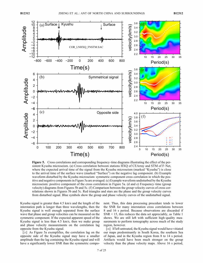
Kyushu signal is greater than 4.5 km/s and the length of theinterstation path is longer than three wavelengths, then theKyushu signal is well enough separated from the surfacewave that phase and group velocities can be measured on thesymmetric component. If the expected apparent speed of theKyushu signal is less than 4.5 km/s, then we make groupand phase velocity measurements on the correlation lagopposite from the Kyushu signal.[23] As Figure 5a exemplifies, the correlation lag on the

opposite side of the Kyushu signal may have a smalleramplitude than the lag containing the Kyushu signal and willhave a significantly lower SNR than the symmetric compo-

nent. Thus, this data processing procedure tends to lowerthe SNR for many interstation cross correlations between8 and 16 s period. Because observations are discarded ifSNR < 15, this reduces the data set appreciably, as Table 1shows. We are still left with sufficient high‐quality mea-surements to perform tomography across much of the studyregion, however.[24] If left untreated, the Kyushu signal would have vitiated

our maps predominantly in South Korea, the southern Seaof Japan, and in the Kyushu region from 8 to 14 s period.Artifacts would have been much stronger on the groupvelocity than the phase velocity maps. Above 16 s period,

Figure 5. Cross correlations and corresponding frequency‐time diagrams illustrating the effect of the per-sistent Kyushu microseism. (a) Cross correlation between stations HXQ of CEArray and STM of F‐Net,where the expected arrival time of the signal from the Kyushu microseism (marked “Kyushu”) is closeto the arrival time of the surface wave (marked “Surface”) on the negative lag component. (b) Examplewaveform disturbed by the Kyushu microseism: symmetric component cross correlation in which the pos-itive and negative components in Figure 5a are averaged. (c) Example waveform undisturbed by the Kyushumicroseism: positive component of the cross correlation in Figure 5a. (d and e) Frequency‐time (groupvelocity) diagrams from Figures 5b and 5c. (f ) Comparison between the group velocity curves of cross cor-relations shown in Figures 5b and 5c. Red triangles and stars are the phase and the group velocity curvesfrom disturbed signal. Blue symbols show the group and phase velocity curves of the undisturbed signal.


7 of 25

however, even if left untreated, the Kyushu signal would havehad only a weak effect on the estimated maps.

4. Rayleigh Wave Dispersion Maps

4.1. Construction of the Dispersion Maps

[25] Surface wave tomography is applied to the selecteddispersion measurements to produce Rayleigh wave groupand phase speed maps on a 0.5° × 0.5° grid using the raytheoretic method of Barmin et al. [2001]. Being mostlydetermined over regional (nonteleseismic) interstation dis-tances, the dispersion measurements observed here will notbe affected strongly by off–great circle effects [e.g., Lin et al.,2009] except for relatively long paths undergoing a conti-nent‐ocean transition. This will primarily affect paths fromJapanese F‐Net to Chinese stations and the maps of the Seaof Japan may be degraded somewhat by this effect. Finitefrequency effects will also be weak in the period band ofstudy [Lin et al., 2011]. The tomographic method of Barminet al. is based on minimizing a penalty functional composedof a linear combination of data misfit, model smoothness, andmodel amplitude. The choice of the damping parameters isbased on the optimization of data misfit and the recovery ofcoherent model features. Due to a shortage of measurements,we are unable to produce reliable maps below 8 s period andabove about 45 s period. The resulting Rayleigh wave dis-persion maps, therefore, are constructed between 8 and 45 son a 2 s period grid.[26] During tomography, resolution is also estimated via

the method described by Barmin et al. [2001] with mod-ifications presented by Levshin et al. [2005]. Resolution isdefined as twice the standard deviation of a 2‐D Gaussian fitto the resolution surface at each geographic node. Examplesof resolution maps are plotted in Figure 6 for the 16 s and 35 speriod measurements. Resolution is estimated to be about100 km across most of the region of study but degrades to200–400 km near the boundary of our studied area wherestation coverage is sparse.[27] Histograms of data misfit using the dispersion maps

at periods of 14 s, 20 s, 30 s, and 40 s are plotted in Figure 7for phase and group velocity. Group travel time misfits are

typically 3–4 times larger than phase travel time misfitsbecause phase velocity measurements are more accurate[Bensen et al., 2007; Lin et al., 2008] and group velocitysensitivity kernels have a larger amplitude. The range ofstandard deviations of the group travel time misfits runsbetween about 4 and 5 s and that of phase travel time betweenabout 1 and 1.5 s. Phase travel timemisfits of ∼1 s between 14and 30 s period are indicative of the quality of the data set,being similar to misfits that result from USArray data [e.g.,Lin et al., 2008].

4.2. Description of the Dispersion Maps

[28] Group and phase velocity maps at periods of 12, 20,30, and 40 s are plotted in Figures 8 and 9. Only those areaswhere the spatial resolution is better than 400 km are shown.The 100 km spatial resolution contour is also plotted as acontinuous white line. Because the 3‐Dmodel is discussed inconsiderable detail in section 6, discussion of the dispersionmaps here is brief but is illuminated by the sensitivity kernelsshown in Figure 10. Both phase (solid lines) and groupvelocity (dashed lines) kernels are shown, computed for 10and 40 s period at two locations in the final model constructedhere: (1) Sea of Japan and (2) North China Craton.[29] As Figure 10 illustrates, at each period the group

velocity measurements are sensitive to shallower structuresthan the phase velocities. Phase velocity maps, therefore,generally should be compared with somewhat shorter‐periodgroup velocity maps. Thus, comparison between Figures 8and 9 reveals that the phase velocity map at 12 s is similarto the group velocity map at 20 s and the phase velocity mapat 20 s is quite like the group velocity pattern at 30 s. Becauseof the lower uncertainty in the phase velocity measurements,however, the phase velocity maps generally are more accu-rate than the maps of group velocity.[30] The dispersion maps are sensitive to quite different

structures between short and long periods and between con-tinental and oceanic regions even at the same period asFigure 10 illustrates. The short‐period dispersion maps (12 sgroup and phase velocity in Figures 8 and 9) are primarilysensitive to upper crustal velocities in continental areas,which are dominated by the presence or lack of sediments.

Figure 6. Resolution estimates at periods of 16 and 35 s, presented in units of kilometers and defined astwice the standard deviation of a 2‐DGaussian fit to the resolution surface at each geographic node [Barminet al., 2001]. The black box shows the region of study.


8 of 25

In regions with oceanic crust, sensitivity is predominantly touppermost mantle structure. At intermediate periods (20 sphase velocity, 20–40 s group velocity), the maps are mostlysensitive to middle to lower crustal velocities beneath con-tinents and continent‐ocean crustal thickness variations. Atlong periods (30–40 s phase velocity), the maps predomi-nantly reflect crustal thickness variations on the continent anduppermost mantle conditions beneath oceans.[31] At short periods (12 s), the dispersion maps in

Figures 8 and 9 exhibit low‐velocity anomalies where sedi-ments are present [Bassin et al., 2000], e.g., the SongliaoBasin (SLB), Huabei Basin (HB), Bohai Bay (BH),North China Platform (NC), the Yellow Sea (ESYS), andthe Tsushima Basin (TB) in the southern Sea of Japan. Theyounger, Cenozoic age sediments of Bohai Bay and theHuabei Basin of theNorth China Craton aremuch slower thanthe older, largely Mesozoic age sediments of the SongliaoBasin. Higher velocities are imaged in the mountains sur-rounding the basins, e.g., the Great Xing’an Range (GXAR),Lesser Xing’an Range (LXAR), the Changbai Mountains(CBM), the Yinshan Mountains (YSM), and the TaihangMountains (THM), which is consistent with the presenceof crystalline rocks near the surface. Weak positive anom-alies are observed in the Korean Peninsula.[32] At intermediate periods (20 s phase velocity, 20–30 s

group velocity), relatively low wave speeds are still observed

for the deeper basins: Songliao, Huabei, Bohai Bay, andYellow Sea. Group and phase velocity are very high in theSea of Japan reflecting oceanic mantle lithospheric shearwave speeds that clearly outline the continental boundary ofthe oceanic crust. It should be noted that off–great circleeffects that may exist are not severe enough to distort theborders of the oceanic crust badly. A significant low‐velocityanomaly appears in Xing’an–East Mongolia. The anomalydoes not develop along the Tancheng‐Lujiang Fault, how-ever, but rather to the west of the Songliao Basin, encom-passing the Great Xing’an Range and the Yinshan Mountainsnorth of the Ordos Block. To the east of the North‐SouthGravity Lineament the crust is much thinner than to its west[e.g., Xu, 2007].[33] For group velocity at 40 s and phase velocity at periods

of 30–40 s, four principal observations are worth noting.First, the high wave speed anomalies of the Sea of Japandiminish from 30 s to 40 s period on the phase velocity maps.This reflects relatively thin lithosphere beneath the Sea ofJapan and increased sensitivity to the underlying astheno-sphere by the longer‐period waves. Second, the Songliao,Huabei, and Bohai basins are situated within the Songliao‐Bohai Graben, which is believed to have formed by back‐arcextension and potential rifting [Liu et al., 2001]. This graben,extending from the Songliao Basin into Bohai Bay, is asso-ciated with a continuous high‐velocity anomaly, which is

Figure 7. Misfit histograms at periods 14, 20, 30, and 40 s. (top) The group velocity misfit and (bottom)the phase velocity misfits. The standard deviations are shown in each panel.


9 of 25

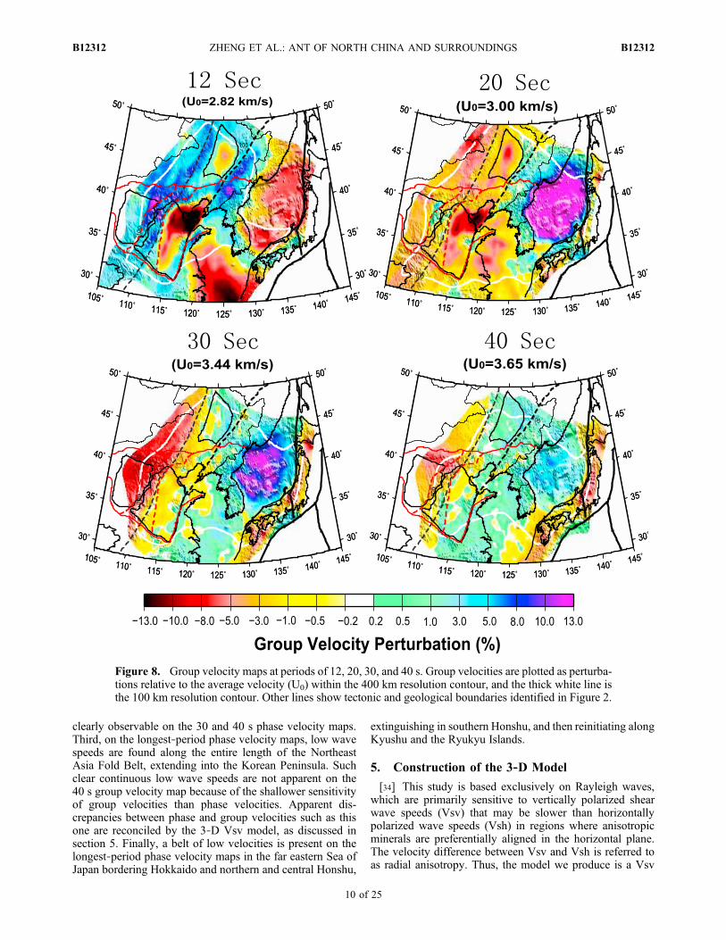
clearly observable on the 30 and 40 s phase velocity maps.Third, on the longest‐period phase velocity maps, low wavespeeds are found along the entire length of the NortheastAsia Fold Belt, extending into the Korean Peninsula. Suchclear continuous low wave speeds are not apparent on the40 s group velocity map because of the shallower sensitivityof group velocities than phase velocities. Apparent dis-crepancies between phase and group velocities such as thisone are reconciled by the 3‐D Vsv model, as discussed insection 5. Finally, a belt of low velocities is present on thelongest‐period phase velocity maps in the far eastern Sea ofJapan bordering Hokkaido and northern and central Honshu,

extinguishing in southern Honshu, and then reinitiating alongKyushu and the Ryukyu Islands.

5. Construction of the 3‐D Model

[34] This study is based exclusively on Rayleigh waves,which are primarily sensitive to vertically polarized shearwave speeds (Vsv) that may be slower than horizontallypolarized wave speeds (Vsh) in regions where anisotropicminerals are preferentially aligned in the horizontal plane.The velocity difference between Vsv and Vsh is referred toas radial anisotropy. Thus, the model we produce is a Vsv

Figure 8. Group velocity maps at periods of 12, 20, 30, and 40 s. Group velocities are plotted as perturba-tions relative to the average velocity (U0) within the 400 km resolution contour, and the thick white line isthe 100 km resolution contour. Other lines show tectonic and geological boundaries identified in Figure 2.


10 of 25

model. In the presence of substantial radial anisotropy, Vsvcan be several percent lower than the effective isotropic shearwave speed, versus Radial anisotropy is common in boththe mantle [e.g., Ekstrom and Dziewonski, 1997; Shapiroand Ritzwoller, 2002] and the crust [e.g., Shapiro et al.,2004; Moschetti et al., 2010a, 2010b], and is geographi-cally variable. We will generally refer to our 3‐D model asbeing a Vsv model, but for simplicity will also refer to it as ashear wave speed or Vs model.[35] The 3‐D Vsv model is based on the Rayleigh wave

phase and group speed maps from 8 to 45 s period on a 0.5° ×0.5° grid across the study region. Periods at which resolutionis greater than 200 km are not included in the inversion. Thisdetermines the outline of the model and in oceanic regions

local dispersion curves typically begin at 12 s period. Localdispersion curves from the eight locations identified with reddots in Figure 2 are shown in Figure 11 with error bars. Thegroup velocity and phase velocity curves shown in Figure 11are mostly smoothly varying and are able to be fit by a ver-tically simple Vs model at each point within observationalerror. In particular, the group and phase velocity curves arereconcilable at each point. Local misfit is presented for eachpoint in Figure 11, where “RMSmisfit”means the square rootof the reduced chi‐square value:

RMSmisfit ¼ 1

N

Xi

di � pið Þ2�2i

" #12

ð1Þ

Figure 9. Same as Figure 8 but for phase velocity maps at periods of 12, 20, 30 and 40 s.


11 of 25

Figure 10. Rayleigh wave phase (solid lines) and group (dashed lines) velocity sensitivity kernels for 10 s(red lines) and 40 s (black lines) periods. (a) Kernels are based on our 3‐D model in the Sea of Japan (pointH, Figure 2). (b) Kernels are based on our 3‐D model in the North China Craton (point B, Figure 2). Thehorizontal black lines denote local Moho depth at each point.

Figure 11. (a–h) Phase and group velocity observations at the eight locations identified with letters inFigure 2, presented with error bars intended to be 1s. The dispersion curves are predicted by the centerof the ensemble of models shown in Figure 12 for each location, with red lines being phase velocity and bluelines group velocity. The RMS misfits are calculated by equation (1).


12 of 25

where di is the observed group or phase velocity value, pi isthe value predicted from the model, si is the uncertainty forthe observation, andN is the total number of phase plus groupvelocity values along the dispersion curves.[36] Uncertainties in phase and group velocity curves are

notoriously difficult to determine reliably, as they are typi-cally underestimated by most tomographic codes based onstandard error propagation [e.g., Barmin et al., 2001]. Theycan be estimated reliably by using the eikonal tomographymethod [Lin et al., 2009], but the method requires moreuniform array spacing than exists in the study region.Therefore, the uncertainties shown in Figure 11 are not fromthe data set presented here, but, as discussed in section 2,misfit statistics in the present study are similar to those thatemerge in the western U.S. based on the regularly spacedUSArray Transportable Array. For this reason, we take theaverage uncertainties estimated by eikonal tomography usingUSArray in the western U.S., but to be conservative wedouble them [Lin et al., 2009;Moschetti et al., 2010a, 2010b].[37] The 3‐D model is constructed via a Monte Carlo

method that is similar to the methods of Shapiro andRitzwoller [2002] and Yang et al. [2008a, 2008b]. The start-ing model for the Monte Carlo search derives from the Vsvvalues of the global model of Shapiro and Ritzwoller [2002]with two principal modifications. First, we simplify thestarting crustal model considerably: the two sedimentarylayers and three crystalline crustal layers of the model ofShapiro and Ritzwoller are averaged separately to define onlytwo constant velocity layers (not including a possible waterlayer). Second, crustal thickness is not allowed to be less than20 km in the Sea of Japan, as discussed in section 6.1. Uni-formly distributed perturbations in Vsv are considered using asingle sedimentary layer with variable thickness and shearvelocity, four B‐splines for Vsv in the crystalline crust, andfive B‐splines in the mantle to a depth of 150 km, belowwhich the model is a constant velocity half‐space. Theresulting model is vertically smooth in both the crystallinecrust and mantle. Moho depth is allowed to vary in a uniforminterval of ±10 km relative to the starting model. Vsv isconstrained to increase monotonically in the crystalline crustand the depth derivative of velocity directly below Moho isconstrained to be positive (i.e., velocity increases with depthright below Moho, but can decrease deeper into the mantle).Both constraints are introduced to reduce the model space, inparticular themagnitude of the trade‐off betweenMoho depthwith structures at depths adjacent to Moho. The positivityconstraint on the depth derivative of velocity in the uppermostmantle typically introduces a thin low velocity “sill” rightbelow Moho, which is an artifact of the constraint.[38] The model has no radial anisotropy, thus Vs = Vsh =

Vsv. Also, we assume that the crystalline crust andmantle is aPoisson solid and set Vp = 1.73Vs, in the sediments we useVp = 2.0Vs, and for density we use the scaling relationadvocated by Christensen and Mooney [1995]: r = 0.541 +0.3601Vp, where r is in g/cm3 and Vp is in km/s. We applya physical dispersion correction [Kanamori and Anderson,1977] using the Q model from PREM [Dziewonski andAnderson, 1981], and the resulting model is reduced to 1 speriod. Offshore, the water depth is recalculated based on a0.2° × 0.2° average of bathymetry at each point.[39] Models are chosen randomly guided by a Metropolis

algorithm [e.g., Mosegaard and Tarantola, 1995] and are

accepted if the reduced c2 misfit to the dispersion curves isless than twice the minimum misfit, cmin

2 , at each location.Reduced c2 misfit is the square of RMS misfit defined byequation (1). RMS misfit averages less than 1.0 across theregion of study. Much of this misfit results from groupvelocities at short periods.[40] As examples, the procedure yields the eight ensembles

of models presented in Figure 12 derived from the eight pairsof Rayleigh wave dispersion curves shown in Figure 11. Theensemble is represented by the gray shaded region, whichpresents two standard deviations (2s) around the mean ateach depth in each direction. The dispersion curves predictedby the best fitting model are shown in Figure 11 as the blue(group velocity) and red (phase velocity) lines. At each depth,the Vsv model that we plot in subsequent figures and itsuncertainty are defined by the middle and one standarddeviation of the ensemble, respectively. The quarter width ofthe ensemble is approximately one standard deviation (1s).The uncertainties in the model are largest where shear wavespeeds trade‐off effectively with boundary topography,which occurs near free boundaries in the model: Mohoand the base of the sedimentary layer. Thus, uncertaintiestypically grow near the top of the crystalline crust and bothabove and below Moho.[41] The eight examples of dispersion curves and the

ensembles of models that fit them, presented in Figures 11and 12, demonstrate how vertically smooth models withtwo discontinuities can fit the data well across the studyregion. A closer inspection of the model profiles, however,reveals the limitations of inversion methods based exclu-sively on surface waves. In particular, the model is affectedby the starting model around which the Monte Carlo methodsamples, particularly sedimentary thickness and crustalthickness.[42] On the continent, input model dependence is most

important beneath sedimentary basins where our simpleparameterization of sedimentary velocities may not faithfullyrepresent local structure. A potential example of this is shownin Figure 12e, beneath the Songliao Basin. Model velocitiesbeneath the basin are very low (∼3.2 km/s) in the crystallineupper crust, which causes a large vertical crustal velocitygradient that may not be realistic. Thus, errors in the inputmodel and the simplicity of parameterization of sedimentarystructure may bias Vs low in the upper crystalline crust. Forthis reason, we do not interpret the resulting 3‐D model atdepths above the lower crust. Imposition of constraints fromreceiver functions would help to resolve this issue, but isbeyond the scope of this work.[43] In the ocean, in contrast, crustal thickness in the

starting model is more poorly known than on the continent.Surprisingly, however, the resulting model is fairly inde-pendent of the starting model. This is illustrated by Figure 13,which shows the resulting ensemble of models for a pointin the Sea of Japan with two different starting models inwhich Moho is at 8 km (Figure 13a) or 20 km (Figure 13b),respectively. In both cases the surface wave data are fitadmirably and nearly identically (e.g., Figure 12h). Withdifferent starting Moho depths of 8 km and 20 km, estimatedmantle velocities at 20 km depth are nearly identical in thetwo ensembles. Crustal velocities and crustal thicknessesdiffer somewhat (average is 13 km and 15 km, respectively),but are within estimated error. Although crustal thickness


13 of 25

may vary from 10 km [Sato et al., 2004] to more than 20 km[Kurashimo et al., 1996] across the Sea of Japan, by settingthe starting Moho depth to 20 km we are able to estimatemantle velocities reliably and recover crustal velocities andthicknesses to within estimated errors. Further discussion ofcrustal thickness beneath the Sea of Japan is presented insection 6.2, which describes the observed anticorrelationbetween crustal thickness and seafloor depth and providesfurther support for the argument that crustal thickness is rel-atively well determined beneath the area.[44] A terminological issue may require clarification.

By “crustal thickness” we mean the thickness of the crustincluding surface topography and a water layer if it exists. By

“Moho depth, ”we mean the depth to Moho below the geoid.By “solid crustal thickness” we refer to the thickness of thecrust not including a water layer.[45] Results from the individual vertical profiles are

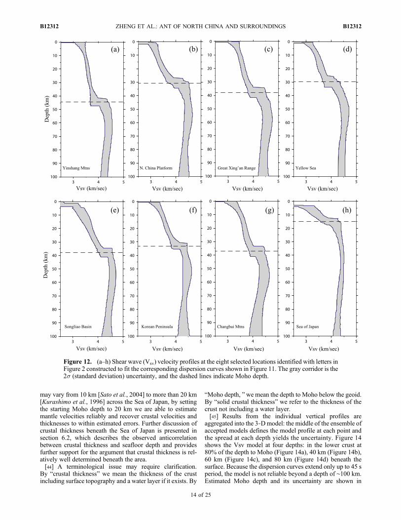
aggregated into the 3‐Dmodel: the middle of the ensemble ofaccepted models defines the model profile at each point andthe spread at each depth yields the uncertainty. Figure 14shows the Vsv model at four depths: in the lower crust at80% of the depth to Moho (Figure 14a), 40 km (Figure 14b),60 km (Figure 14c), and 80 km (Figure 14d) beneath thesurface. Because the dispersion curves extend only up to 45 speriod, the model is not reliable beyond a depth of ∼100 km.Estimated Moho depth and its uncertainty are shown in

Figure 12. (a–h) Shear wave (Vsv) velocity profiles at the eight selected locations identified with letters inFigure 2 constructed to fit the corresponding dispersion curves shown in Figure 11. The gray corridor is the2s (standard deviation) uncertainty, and the dashed lines indicate Moho depth.


14 of 25

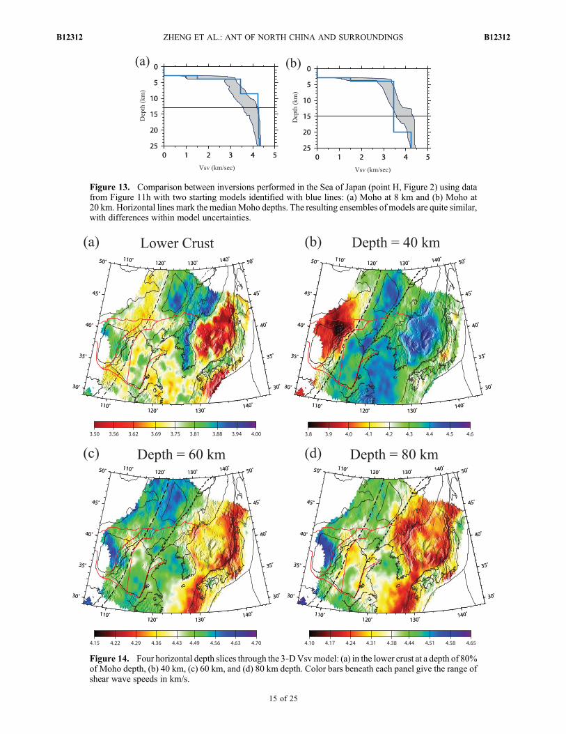
Figure 13. Comparison between inversions performed in the Sea of Japan (point H, Figure 2) using datafrom Figure 11h with two starting models identified with blue lines: (a) Moho at 8 km and (b) Moho at20 km. Horizontal lines mark the medianMoho depths. The resulting ensembles of models are quite similar,with differences within model uncertainties.

Figure 14. Four horizontal depth slices through the 3‐DVsvmodel: (a) in the lower crust at a depth of 80%of Moho depth, (b) 40 km, (c) 60 km, and (d) 80 km depth. Color bars beneath each panel give the range ofshear wave speeds in km/s.


15 of 25

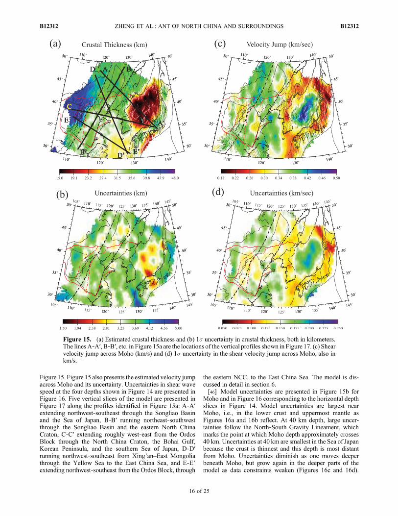
Figure 15. Figure 15 also presents the estimated velocity jumpacross Moho and its uncertainty. Uncertainties in shear wavespeed at the four depths shown in Figure 14 are presented inFigure 16. Five vertical slices of the model are presented inFigure 17 along the profiles identified in Figure 15a: A‐A′extending northwest‐southeast through the Songliao Basinand the Sea of Japan, B‐B′ running northeast‐southwestthrough the Songliao Basin and the eastern North ChinaCraton, C‐C′ extending roughly west‐east from the OrdosBlock through the North China Craton, the Bohai Gulf,Korean Peninsula, and the southern Sea of Japan, D‐D′running northwest‐southeast from Xing’an–East Mongoliathrough the Yellow Sea to the East China Sea, and E‐E’extending northwest‐southeast from the Ordos Block, through

the eastern NCC, to the East China Sea. The model is dis-cussed in detail in section 6.[46] Model uncertainties are presented in Figure 15b for

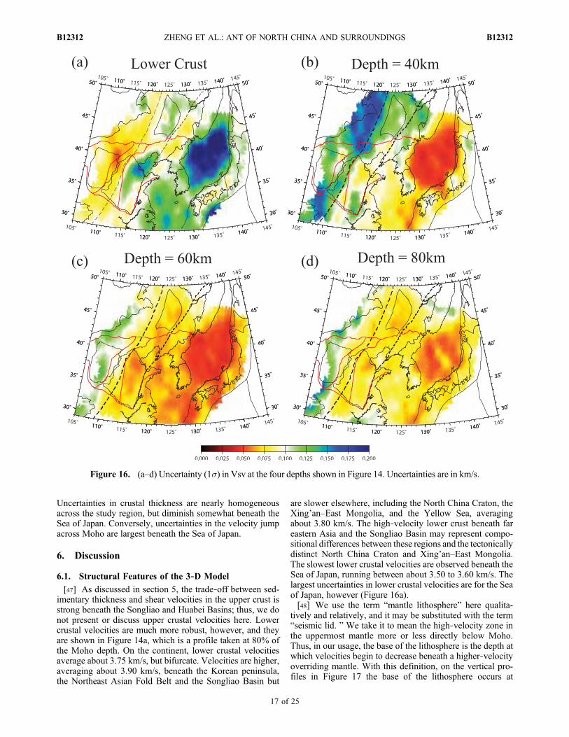
Moho and in Figure 16 corresponding to the horizontal depthslices in Figure 14. Model uncertainties are largest nearMoho, i.e., in the lower crust and uppermost mantle asFigures 16a and 16b reflect. At 40 km depth, large uncer-tainties follow the North‐South Gravity Lineament, whichmarks the point at which Moho depth approximately crosses40 km. Uncertainties at 40 km are smallest in the Sea of Japanbecause the crust is thinnest and this depth is most distantfrom Moho. Uncertainties diminish as one moves deeperbeneath Moho, but grow again in the deeper parts of themodel as data constraints weaken (Figures 16c and 16d).

Figure 15. (a) Estimated crustal thickness and (b) 1s uncertainty in crustal thickness, both in kilometers.The lines A‐A′, B‐B′, etc. in Figure 15a are the locations of the vertical profiles shown in Figure 17. (c) Shearvelocity jump across Moho (km/s) and (d) 1s uncertainty in the shear velocity jump across Moho, also inkm/s.


16 of 25

Uncertainties in crustal thickness are nearly homogeneousacross the study region, but diminish somewhat beneath theSea of Japan. Conversely, uncertainties in the velocity jumpacross Moho are largest beneath the Sea of Japan.

6. Discussion

6.1. Structural Features of the 3‐D Model

[47] As discussed in section 5, the trade‐off between sed-imentary thickness and shear velocities in the upper crust isstrong beneath the Songliao and Huabei Basins; thus, we donot present or discuss upper crustal velocities here. Lowercrustal velocities are much more robust, however, and theyare shown in Figure 14a, which is a profile taken at 80% ofthe Moho depth. On the continent, lower crustal velocitiesaverage about 3.75 km/s, but bifurcate. Velocities are higher,averaging about 3.90 km/s, beneath the Korean peninsula,the Northeast Asian Fold Belt and the Songliao Basin but

are slower elsewhere, including the North China Craton, theXing’an–East Mongolia, and the Yellow Sea, averagingabout 3.80 km/s. The high‐velocity lower crust beneath fareastern Asia and the Songliao Basin may represent compo-sitional differences between these regions and the tectonicallydistinct North China Craton and Xing’an–East Mongolia.The slowest lower crustal velocities are observed beneath theSea of Japan, running between about 3.50 to 3.60 km/s. Thelargest uncertainties in lower crustal velocities are for the Seaof Japan, however (Figure 16a).[48] We use the term “mantle lithosphere” here qualita-

tively and relatively, and it may be substituted with the term“seismic lid. ” We take it to mean the high‐velocity zone inthe uppermost mantle more or less directly below Moho.Thus, in our usage, the base of the lithosphere is the depth atwhich velocities begin to decrease beneath a higher‐velocityoverriding mantle. With this definition, on the vertical pro-files in Figure 17 the base of the lithosphere occurs at

Figure 16. (a–d) Uncertainty (1s) in Vsv at the four depths shown in Figure 14. Uncertainties are in km/s.


17 of 25

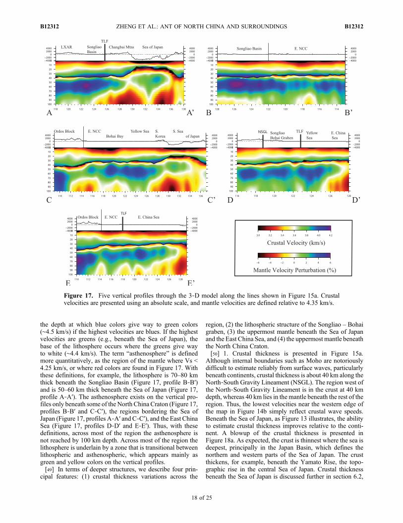
the depth at which blue colors give way to green colors(∼4.5 km/s) if the highest velocities are blues. If the highestvelocities are greens (e.g., beneath the Sea of Japan), thebase of the lithosphere occurs where the greens give wayto white (∼4.4 km/s). The term “asthenosphere” is definedmore quantitatively, as the region of the mantle where Vs <4.25 km/s, or where red colors are found in Figure 17. Withthese definitions, for example, the lithosphere is 70–80 kmthick beneath the Songliao Basin (Figure 17, profile B‐B′)and is 50–60 km thick beneath the Sea of Japan (Figure 17,profile A‐A′). The asthenosphere exists on the vertical pro-files only beneath some of the North China Craton (Figure 17,profiles B‐B′ and C‐C′), the regions bordering the Sea ofJapan (Figure 17, profiles A‐A′ and C‐C′), and the East ChinaSea (Figure 17, profiles D‐D′ and E‐E′). Thus, with thesedefinitions, across most of the region the asthenosphere isnot reached by 100 km depth. Across most of the region thelithosphere is underlain by a zone that is transitional betweenlithospheric and asthenospheric, which appears mainly asgreen and yellow colors on the vertical profiles.[49] In terms of deeper structures, we describe four prin-

cipal features: (1) crustal thickness variations across the

region, (2) the lithospheric structure of the Songliao – Bohaigraben, (3) the uppermost mantle beneath the Sea of Japanand the East China Sea, and (4) the uppermost mantle beneaththe North China Craton.[50] 1. Crustal thickness is presented in Figure 15a.

Although internal boundaries such as Moho are notoriouslydifficult to estimate reliably from surface waves, particularlybeneath continents, crustal thickness is about 40 km along theNorth‐South Gravity Lineament (NSGL). The region west ofthe North‐South Gravity Lineament is in the crust at 40 kmdepth, whereas 40 km lies in the mantle beneath the rest of theregion. Thus, the lowest velocities near the western edge ofthe map in Figure 14b simply reflect crustal wave speeds.Beneath the Sea of Japan, as Figure 13 illustrates, the abilityto estimate crustal thickness improves relative to the conti-nent. A blowup of the crustal thickness is presented inFigure 18a. As expected, the crust is thinnest where the sea isdeepest, principally in the Japan Basin, which defines thenorthern and western parts of the Sea of Japan. The crustthickens, for example, beneath the Yamato Rise, the topo-graphic rise in the central Sea of Japan. Crustal thicknessbeneath the Sea of Japan is discussed further in section 6.2,

Figure 17. Five vertical profiles through the 3‐D model along the lines shown in Figure 15a. Crustalvelocities are presented using an absolute scale, and mantle velocities are defined relative to 4.35 km/s.


18 of 25

where the anticorrelation observed between crustal thick-ness and water depth is used to support the reliability of thecrustal thickness estimates in oceanic regions.[51] 2. At 40 km depth east of the North‐South Gravity

Lineament relatively high wave speeds (>4.4 km/s) liebeneath the Songliao Basin and run to the Bohai Sea, asFigure 14b shows. The high velocities beneath the SongliaoBasin form a lid that extends to 60–70 km but then terminates,being underlain by more normal continental uppermostmantle wave speeds beneath the Basin by 80 km depth. Thiscan be seen clearly on vertical profiles A‐A′ and B‐B′ ofFigure 17, in which the relatively thick fast lithospherebeneath the Songliao graben is contrasted with the thinnerslower lithosphere of the North China Craton and the Seaof Japan. The mantle lithosphere, however, beneath theSongliao Basin is not cratonic in nature, contrasting withthe much thicker lithosphere beneath the Ordos Block (e.g.,Figure 14d). Although the Ordos Block is only partiallyimaged in this study, high velocities are seen to underlie itin the uppermost mantle extending at least to 100 km depth(and presumably deeper) as vertical profile C‐C′ in Figure 17illustrates. Although the lithosphere underlying the SongliaoBasin is not as thin as beneath the North China Craton, it isthin for a region believed to have a basement of Archean age.[52] 3. At 40 km depth, relatively high wave speeds

(>4.4 km/s) also underlie the Yellow and Japan Seas.Although similar in the uppermost mantle, below 40 km themantle structures beneath these seas lose their similarity. Theuppermost mantle beneath the Yellow Sea is continental incharacter as profile D‐D′ in Figure 17 shows. Much lowerwave speeds exist in the back‐arc spreading region beneaththe Sea of Japan, as can been seen on Figures 14c and 14d.Starting at about 60 km depth, low velocities bound theeastern margin of the Sea of Japan and also to a somewhat

lesser extent the western margin, extending onto the conti-nent. Low velocities also bound the eastern edge of the EastChina Sea, east and southeast of the Yellow Sea near theRyukyu Islands. By 80 km depth, the bifurcated low‐velocityzone across the Sea of Japan has largely merged into a morehomogeneous low‐velocity asthenosphere beneath the entiresea, and the western edge of the anomaly has spread furtherinland to underlie the Northeast Asia Fold Belt, includingthe volcanic region of the Changbai Mountains. This ispresented most clearly in Figure 19, which displays twolow‐velocity contours at 80 km depth: Vs < 4.25 km/s and4.25 km/s ≤ Vs < 4.35 km/s. This also can be seen clearly inprofile A‐A′ of Figure 17, which extends across the center ofthe Sea of Japan, but is also visible in profile C‐C′ which runthrough the sea farther south. We refer to the low velocitiesbounding the Sea of Japan as a “Y‐shaped” anomaly onvertical profiles, which is apparent on profile A‐A′. A rela-tively high velocity 50–60 km thick lithosphere is observedbeneath the central Sea of Japan, as profiles A‐A′ and C‐C′illustrate. This relatively thin lithosphere should be con-trasted with the thicker faster lithosphere beneath theSongliao Basin, which is clearly seen on profile A‐A′. Thebordering Y‐shaped asthenospheric anomaly and the thinlithosphere underlying the Sea of Japan are discussed fur-ther in section 6.3. The East China Sea lies near the south-eastern corner of our study region, but like the Sea of Japanits eastern margin near the Ryukyu Islands is underlain bylow velocities in the uppermost mantle. This is apparent inFigures 19 and 14d and vertical profile D‐D′ in Figure 17.Unlike the Sea of Japan, however, there is no “Y‐shaped”anomaly beneath the East China Sea as the western part ofthe sea merges with fast continental lithosphere beneath theYellow Sea with no low‐velocity feature in the uppermostmantle.

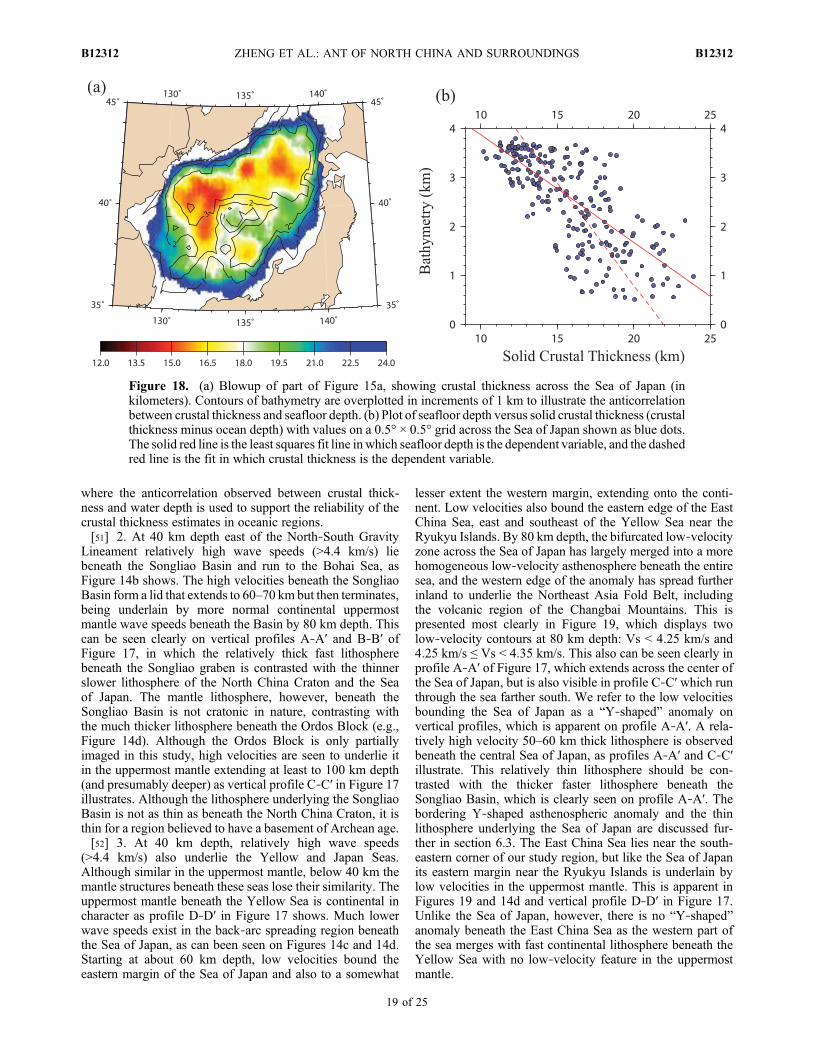
Figure 18. (a) Blowup of part of Figure 15a, showing crustal thickness across the Sea of Japan (inkilometers). Contours of bathymetry are overplotted in increments of 1 km to illustrate the anticorrelationbetween crustal thickness and seafloor depth. (b) Plot of seafloor depth versus solid crustal thickness (crustalthickness minus ocean depth) with values on a 0.5° × 0.5° grid across the Sea of Japan shown as blue dots.The solid red line is the least squares fit line in which seafloor depth is the dependent variable, and the dashedred line is the fit in which crustal thickness is the dependent variable.


19 of 25

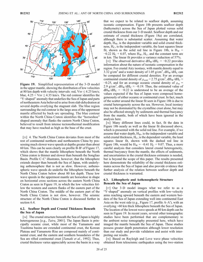
[53] 4. The North China Craton deviates from most of therest of continental northern and northeastern China by pos-sessingmuch slower wave speeds at depths greater than about60 km. This can be seen clearly on profile B‐B′ of Figure 17,which shows that the mantle lithosphere beneath the NorthChina craton is thinner and slower than beneath the SongliaoBasin. Profile C‐C′ illustrates, however, that the lithosphereextends deeper than beneath the Sea of Japan, with underly-ing asthenosphere that is not as slow. However, astheno-spheric wave speeds do underlie the lithosphere beneath theNorth China Craton below about 80 km depth. These lowwave speeds in the uppermost mantle are horseshoe in shapeon horizontal cross sections across the eastern North ChinaCraton as seen in Figure 19, in which the low velocities fol-low the western and eastern flanks of the eastern part of theNorth China Craton. The middle of the eastern part of theNorth China Craton is not slow, however. The seismicstructure of the North China Craton is discussed further insection 6.4.

6.2. Seafloor Depth and Crustal Thickness Beneaththe Sea of Japan

[54] The crustal structure beneath the Sea of Japan is highlyheterogeneous [e.g., Taira, 2001]. The Japan Basin is prin-cipally oceanic crust, while most of the Yamamoto andTsushima basins are extended continental crust, the KoreanPlateau and Yamamoto Rise are composed mainly of conti-nental crust, and the eastern and southern boundaries of theSea are rifted continental crust [Tamaki et al., 1992]. Thus,crustal thickness varies appreciably across the basin in a way

that we expect to be related to seafloor depth, assumingisostatic compensation. Figure 18b presents seafloor depth(bathymetry) across the Sea of Japan plotted versus solidcrustal thickness from our 3‐Dmodel. Seafloor depth and ourestimate of crustal thickness (Figure 18a) are correlated,although there is substantial scatter. Assuming that waterdepth, HW, is the dependent variable and solid crustal thick-ness, HC, is the independent variable, the least squares linearfit, shown as the solid red line in Figure 18b, is HW =−0.22 HC + 6.07, where HW, HC, and the constant term arein km. The linear fit provides a variance reduction of 57%.[55] The observed derivative dHW/dHC = −0.22 provides

information about the nature of isostatic compensation in theregion. For crustal Airy isostasy, with mantle density equal to3.32 g/cm3 and a water density of 1.05 g/cm3, dHW/dHC canbe computed for different crustal densities. For an averagecontinental crustal density of rcont = 2.75 g/cm3, dHW/dHC ≈−0.25, and for an average oceanic crustal density of roc =2.9 g/cm3, dHW/dHC ≈ −0.19. Thus, the estimated value ofdHW/dHC = −0.22 is understood to be an average of thevalues expected if the Sea of Japan were composed homo-geneously of either oceanic or continental crust. In fact, muchof the scatter around the linear fit seen in Figure 18b is due tocrustal heterogeneity across the sea. However, local isostasymay not be dominated by the crystalline crust alone, but mayalso be affected strongly by sediments and thermal buoyancyfrom the mantle, both of which have been ignored in theanalysis here.[56] Many different lines could, in fact, fit the data in

Figure 18b nearly as well as the linear fit discussed above,which is presented with the solid red line. For example, if weassume that water depth, HW, is the independent variable andsolid crustal thickness, HC, is the dependent variable, the leastsquares linear fit, shown with the dashed red line inFigure 18b, would be HW = −0.41 HC + 9.07. Thus, a morecareful analysis that considers lateral crustal heterogeneity,thermal buoyancy from the mantle, the effects of sediments,and uncertainties in the crustal thickness estimates is needed,but is beyond the scope of this paper. The results presentedhere demonstrate the reliability of the crustal thickness esti-mates across the Sea of Japan and also provide evidence thatfurther analysis of the relation between seafloor depth andcrustal thickness is warranted.

6.3. Lithospheric and Asthenospheric StructureBeneath the Sea of Japan

[57] Our 3‐D model images what we refer to as a“Y‐shaped” anomaly on vertical profiles with low‐velocityarms reaching upward beneath the eastern and western bor-ders of the Sea of Japan extending well into continental EastAsia on the west side (e.g., Figure 17, profile A‐A′), with anoverlying ∼60 km thick lithosphere beneath the Sea of Japan.The location of the lowest wave speeds at 80 km depth can beseen in Figure 19. In recent years, several other tomographicstudies have been performed that are complementary tothe ambient noise tomography presented here, which haveimaged the mantle beneath the Sea of Japan. These studiespossess greater depth penetration although lower resolutionthan our study and provide validation and assist with inter-preting our results.[58] Based on Rayleigh and Love wave phase velocities

obtained from teleseismic earthquakes using the two‐station

Figure 19. Simplified representation of the 3‐D modelin the upper mantle, showing the distribution of low velocitiesat 80 km depth with velocity intervals: red, Vsv ≤ 4.25 km/s;blue, 4.25 < Vsv ≤ 4.35 km/s. The red contour identifies the“Y‐shaped” anomaly that underlies the Sea of Japan and partsof northeastern Asia believed to arise from slab dehydration atseveral depths overlying the stagnant slab. The blue regionsurrounding the red contour is the large area of the uppermostmantle affected by back‐arc spreading. The blue contourwithin the North China Craton identifies the “horseshoe”shaped anomaly that flanks the eastern North China Craton,believed to result from intense tectonothermal modificationthat may have reached as high as the base of the crust.


20 of 25

method, Yoshizawa et al. [2010] present a 3‐Dmodel of shearwave speeds from 40 to 200 km depth. Although their reso-lution is best beneath Japan and fades by the central Seaof Japan, their results in regions of good data coverage aresimilar to ours in several respects. First, they report an aver-age lithospheric thickness beneath the Yamato Rise and theJapan Basin of 60 ± 10 km, which is similar to what weobserve (e.g., Figure 17, profiles A‐A′ and C′C′). Second,they also observe low‐velocity anomalies at 75 km depthbordering Honshu beneath the eastern Sea of Japan and theEast China Sea, west of the Ryukyu Islands. Thus, they alsoimage the eastern arm of the Y‐shaped anomaly that we reporthere and, like our model, observe it to migrate westward withdepth. Their data coverage does not extend into East Asia.However, the teleseismic body wave study of Zhao et al.[2007] presented a large‐scale image of the upper mantlebeneath east Asia, which shows the stagnation of thesubducted Pacific Plate beneath the Sea of Japan and clearlow‐velocity anomalies in the back‐arc region. This studyconcentrates interpretation on the release of volatiles from theslab at several depths to produce the low‐velocity anom-alies observed in the back‐arc region.[59] Thus, Yoshizawa et al. [2010] serve to validate our

model and Zhao et al. [2007] provide a means to interpretthe Y‐shaped anomaly based on what they call the “BigMantle Wedge” model of the Japanese back arc and thedevolatilization of the subducted slab. In their interpretation,the western arm of the Y‐shaped anomaly beneath the west-ern Sea of Japan and the East Asian Fold Belt would becaused by dehydration reactions of the stagnant slab in themantle boundary layer (410–660 km). These warm hydratedupwellings are the cause of volcanism in East Asia (e.g.,Changbai volcano) and may have precipitated the crustalrifting that led to the opening of the Sea of Japan. Presumably,the stagnant slab would generate hydrated plumes across theentire Sea of Japan, but the stretched and thinned continentallithosphere remains intact beneath the central Sea of Japan,as Figure 17 profiles A‐A′ and C‐C′ demonstrate, impedingupward migration of the hydrated plumes. These plumeswould then become part of a westward directed convectingsystem that would amplify mantle hydration in the westernSea of Japan, near the rift margin. The eastern arm of theY‐shaped anomaly would be caused by slab dehydrationat shallower depths, possibly caused by antigorite‐relatedreactions. Thus, the Y‐shaped anomaly reflects the detailsof shallow and deep slab dehydration and convective circu-lation in the mantle wedge above a stagnant slab.

6.4. Lithospheric Rejuvenation of the North ChinaCraton

[60] The Chinese part of the Sino‐Korean Craton, called theNorth China Craton (NCC), is composed of two Archeanblocks, the eastern and the western NCC, which are separatedby the central NCC. The central NCC is a Paleoproterozoicorogen called the Trans‐North China Orogen. The three partsof the NCC are separated by dashed red lines in Figure 2. TheNCC is believed to have cratonized by about 1.85 Ga, butthe eastern NCC has undergone significant tectonothermalrejuvenation from the Ordovician to Cenozoic [Menzies et al.,1993, 2007;Griffin et al., 1998;Gao et al., 2002, 2004; Zhaoet al., 2005, 2008]. These conclusions have been based onbasalt‐borne xenoliths and geophysical evidence for thin

lithosphere (<100 km) with high heat flow in this region fromthe early Cenozoic to the present [e.g., Menzies et al., 1993;Griffin et al., 1998; Fan et al., 2000; Xu, 2001; Wu et al.,2005; Chen et al., 2006, 2008, 2009]. Most studies agreethat the central and western parts of the NCC have evolveddifferently than the eastern NCC during Phanerozoic time[e.g., Xu et al., 2004;Xu, 2007], although some recent seismicstudies point to localized lithospheric thinning in the centraland even western NCC [e.g., Huang et al., 2009; Chen et al.,2009] and the generally high lateral heterogeneity of thelithosphere underlying the NCC. The mechanism of Phan-erozoic lithospheric rejuvenation and its variability across theNCC remain intensely debated (see, e.g., Chen [2010] for arecent summary). Understanding of the Phanerozoic litho-spheric tectonics would be improved with clearer imagesof the current structure of the crust, mantle lithosphere, andasthenosphere across the NCC.[61] To this debate our 3‐D model presents new relatively

high‐resolution images of the crust and uppermost mantlebeneath most of the NCC. Crustal velocities beneath theeastern NCC are not particularly distinct from surroundingregions (e.g., Figure 14a), although the crust may be slightlythinner, on average (Figure 15a). More significantly, theeastern NCC hosts a “horseshoe” shaped anomaly in mapview in the uppermost mantle, which is identified at 80 kmdepth in Figure 14d and, perhaps more clearly, by the bluecontour in Figure 19. The velocities are lowest in the northernpart of the North China Platform near the intersection of theNorth‐South Gravity Lineament (NSGL) with the boundarybetween the central and eastern NCC. The low velocitiescontinue southward, flanking the eastern NCC along theNSGL in the west and the TLF in the east. Low velocities alsoextend into small parts of the central NCC and the westernNCC near the DatongVolcanoes. The south central part of theNCC is not particularly slow in the uppermost mantle asFigure 17 profile E‐E′ illustrates, which reveals the consid-erable variability of lithospheric structure even within theeastern NCC.[62] Within the “horseshoe” shaped anomaly bounding

three sides of the eastern NCC (Figure 19), the lithospherecan be seen to be about 60 km thick on vertical profiles B‐B′and C‐C′ of Figure 17. The flanks of the eastern NCC areunderlain by asthenospheric low‐velocity anomalies below70 km depth as can be seen on profiles B‐B′, C‐C′, and E‐E′.Profile B‐B′ illustrates that the lithosphere is not simply thin;the velocities are lower than beneath the Songliao Basin to thenorth and the Ordos Block to the west. Thus, we hypothesizethat the low‐velocity anomalies that bound three sides of theeastern NCC identify a region of more intense tectonothermalactivity than in south central part of the eastern NCC. Indeed,lithospheric rejuvenation may have reached nearly to the baseof the crust in the most intensely altered zones.

7. Conclusions

[63] This paper presents a high‐resolution 3‐D shearvelocity model of the crust and uppermost mantle withassociated uncertainties across the North China Craton,northeastern China, the Korean Peninsula, and the Sea ofJapan constructed from the dispersion characteristics ofRayleigh waves obtained from ambient noise cross correla-tions. Broadband stations from Chinese Provincial Networks,


21 of 25

the Japanese F‐Net, and the IRIS GSN have produced 2 yearcontinuous time series from 2007 into 2009 that form thebasis for these results. Phase and group velocity maps from8 s to 45 s period are first constructed, which constrain earthstructures in the crust and uppermost mantle to a depth ofabout 100 km. The dispersion maps are geologically coher-ent, displaying the signatures of sedimentary basins, moun-tain roots, ocean‐continent variations, and anomalies due torifting and volcanism. The maps at different periods andbetween phase and group velocities are consistent with oneanother, and vertically relatively smooth Vsv models fit theobservations.[64] To generate the dispersion maps presented here, the

effects of the persistent localized Kyushu microseism had tobe eliminated in the dispersion measurements. We present amethod based on locating the microseism (thereby confirm-ing the location of Zeng and Ni [2010]), predicting the arrivalof the disturbing signal on the ambient noise cross correla-tions, and obtaining the dispersion measurements by usingthe Green’s functions at the opposite cross‐correlation lagtimes for the station pairs in which the apparent speed of theKyushu signal is less than 4.5 km/s.[65] Ambient noise tomography places unique constraints

on the structure of the crust and uppermost mantle, provid-ing information complementary to body wave travel times,receiver functions, longer‐period teleseismic surface waves,gravity, and other types of data. The motivation for the 3‐Dmodel is to produce new constraints on the volcanism, crustalextension, cratonic rejuvenation, and lithospheric thinningthat are hypothesized for the region of study. The modelpresented here provides new information about these pro-cesses, particularly about the geometry (the geographic dis-tribution and depth extent) of the observed features in the top100 km. A detailed interpretation of the model is inconsistentwith the scope of this paper, but we focus discussion onfour principal model features: crustal thickness variations,particularly those associated with the North‐South GravityLineament (NSGL) and beneath the Sea of Japan, theprominent but thin lithosphere underlying the Songliao‐Bohai Graben, the “Y‐shaped”mantle low‐velocity anomaly(on vertical profiles) bordering the Sea of Japan, and a“horseshoe” shaped asthenospheric anomaly (in map view)bounding three sides of the eastern North China Craton.[66] 1. The North‐South Gravity Lineament is observed to

follow approximately the 40 km crustal thickness contour.Beneath the Sea of Japan, crustal thickness is anticorrelatedwith water depth, and the relationship is consistent withexpectations based on crustal isostasy for a laterally compo-sitionally variable crust.[67] 2. The Songliao‐Bohai Graben is underlain by a high‐

velocity lower crust and a fast mantle lithosphere that extendsto about 70 km depth. The lithosphere is not attenuated; thatis seismic velocities are high, but it is thinner than expectedfor a region in which parts are traceable back to the Archean.[68] 3. Low‐velocity anomalies reach upward beneath the

eastern and western borders of the Sea of Japan, extendingwell into continental East Asia on the west side. The arms ofthis Y‐shaped anomaly are separated by the interveningoverlying lithosphere, which is ∼60 km thick and may rep-resent stretched continental lithosphere. We argue that theY‐shaped structure in the east reflects relatively shallow

slab dehydration and in the west deeper dehydration andconvective circulation in the mantle wedge overlying thestagnant slab.[69] 4. Very thin, attenuated lithosphere bounds three sides

of the eastern North China Craton (NCC), but somewhatthicker faster lithosphere underlies the central and southernparts of the eastern NCC. These low‐velocity anomaliesidentify a region of intense tectonothermal modificationwhere lithospheric rejuvenation may have reached nearlyto the base of the crust.[70] In the future, assimilating similar results from a com-

panion paper for southern China (Zhou et al., submittedmanuscript, 2011) will allow the 3‐D model to extend acrossall of eastern China. The geometry of the observing arraymakes the application of differential travel time methods forearthquakes difficult, such as eikonal tomography [Lin et al.,2009], Helmholtz tomography [Lin and Ritzwoller, 2011],or two‐plane wave tomography [e.g., Yang et al., 2008b].However, the success of such methods would allow disper-sion maps to be extended to longer periods and, therefore, forthe model to reach greater depths in the mantle. In addition tothe production of a 3‐D Vs model of the crust and uppermostmantle, other research envisioned includes the estimation ofazimuthal anisotropy, which would place complementaryconstraints on the physical processes that motive this study.In addition, future understanding of the dispersion char-acteristics of Love waves would allow estimation of radialanisotropy, which reflects deformation undergone by thecrust and uppermost mantle.

[71] Acknowledgments. The authors wish to thank An Yin and ananonymous reviewer for constructive criticism of an early draft and the AEfor particularly insightful comments on a late draft of this paper. Weare grateful to Anatoli Levshin, Fan‐Chi Lin, and Shijie Zhong for valuableconversations. This work was performed while the first author visited theUniversity of Colorado at Boulder over a period of one year. The workwas supported by NSFC grant 40974034, CAS grant kzcx2‐yw‐142 andY009021002, NSFC 41174086, CEA grant 201008007, US NSF‐EARaward 0944022, and US NSF‐OISE sub‐award 0730154. This is contribu-tion 20 from the ARC Centre of Excellence for Core to Crust Fluid Systems(http://www.ccfs.mq.edu.au) and 791 in the GEMOC Key Centre (http://www.gemoc.mq.edu.au). Most of the waveform data for this study wereprovided by the Data Management Centre of the China National SeismicNetwork at the Institute of Geophysics, China Earthquake Administrationand F‐Net in Japan. In addition, the facilities of the IRIS Data ManagementSystem were used to access data required in this study. The IRIS DMS isfunded through the U.S. National Science Foundation under cooperativeagreement EAR‐0552316.

ReferencesBai, L., H. Kawakatsu, and Y. Morita (2010), Two anisotropic layers incentral orogenic belt of the North China Craton, Tectonophysics, 494,138–148, doi:10.1016/j.tecto.2010.09.002.

Barmin, M. P., M. H. Ritzwoller, and A. L. Levshin (2001), A fast and reli-able method for surface wave tomography, Pure Appl. Geophys., 158,1351–1375, doi:10.1007/PL00001225.

Bassin, C., G. Laske, and G. Masters (2000), The current limits of resolu-tion for surface wave tomography in North America, Eos Trans. AGU,81, F897.

Bensen, G. D., M. H. Ritzwoller, M. P. Barmin, A. L. Levshin, F. Lin,M. P. Moschetti, N. M. Shapiro, and Y. Yang (2007), Processing seismicambient noise data to obtain reliable broad‐band surface wave dispersionmeasurements, Geophys. J. Int., 169, 1239–1260, doi:10.1111/j.1365-246X.2007.03374.x.

Bensen, G. D., M. H. Ritzwoller, and N. M. Shapiro (2008), Broad-band ambient noise surface wave tomography across the United States,J. Geophys. Res., 113, B05306, doi:10.1029/2007JB005248.


22 of 25

Bensen, G. D., M. H. Ritzwoller, and Y. Yang (2009), A 3‐D shear velocitymodel of the crust and uppermost mantle beneath the United States fromambient seismic noise, Geophys. J. Int., 177, 1177–1196, doi:10.1111/j.1365-246X.2009.04125.x.

Bourova, E., K. Yoshizawa, and K. Yomogida (2010), Upper mantle struc-ture of marginal seas and subduction zones in northeastern Eurasia fromRayleigh wave tomography, Phys. Earth Planet. Inter., 183, 20–32,doi:10.1016/j.pepi.2010.06.007.

Chen, L. (2010), Concordant structural variations from the surface to thebase of the upper mantle in the North China Craton and its tectonic impli-cations, Lithos, 120, 96–115, doi:10.1016/j.lithos.2009.12.007.

Chen, L., T. Zheng, and W. Xu (2006), A thinned lithospheric image of theTanlu Fault Zone, eastern China: Constructed from wave equation basedreceiver function migration, J. Geophys. Res., 111, B09312, doi:10.1029/2005JB003974.

Chen, L., T. Wang, L. Zhao, and T. Zheng (2008), Distinct lateral variationof lithospheric thickness in the northeastern North China Craton, EarthPlanet. Sci. Lett., 267, 56–68, doi:10.1016/j.epsl.2007.11.024.

Chen, L., C. Cheng, and Z. Wei (2009), Seismic evidence for significantlateral variations in lithospheric thickness beneath the central and westernNorth China Craton, Earth Planet. Sci. Lett., 286, 171–183, doi:10.1016/j.epsl.2009.06.022.

Cho, K. H., R. B. Herrmann, C. J. Ammon, and K. Lee (2007), Imaging theupper crust of the Korean Peninsula by surface‐wave tomography, Bull.Seismol. Soc. Am., 97(1B), 198–207, doi:10.1785/0120060096.

Christensen, N. I., and W. D. Mooney (1995), Seismic velocity structureand composition of the continental crust: A global view, J. Geophys.Res., 100, 9761–9788, doi:10.1029/95JB00259.

Deng, J., S. Su, Y. Niu, C. Liu, G. Zhao, X. Zhao, S. Zhou, and Z. Wu(2007), A possible model for the lithospheric thinning of the North ChinaCraton: Evidence from the Yanshanian (Jura‐Cretaceous) magmatismand tectonism, Lithos, 96, 22–35, doi:10.1016/j.lithos.2006.09.009.

Dziewonski, A. M., and D. L. Anderson (1981), Preliminary referenceEarth model, Phys. Earth Planet. Inter., 25, 297–356, doi:10.1016/0031-9201(81)90046-7.

Ekstrom, G., and A. M. Dziewonski (1997), Three‐dimensional velocitystructure of the Earth’s upper mantle, in Upper Mantle HeterogeneitiesFrom Active and Passive Seismology, edited by K. Fuchs, pp. 187–198,Kluwer Acad., Norwell, Mass.

Fan, W., H. Zhang, J. Baker, K. Jarvis, P. R. D. Mason, and M. Menzies(2000), On and off the North China Craton: Where is the Archaean keel?,J. Petrol., 41(7), 933–950, doi:10.1093/petrology/41.7.933.

Fang, L., J. Wu, Z. Ding, and G. Panza (2010), High resolution Rayleighwave group velocity tomography in North‐China from ambient seismicnoise, Geophys. J. Int., 181, 1171–1182.

Gao, S., R. Rudnick, R. Carlson, W. McDonough, and Y. Liu (2002),Re‐Os evidence for replacement of ancient mantle lithosphere beneaththe North China Craton, Earth Planet. Sci. Lett., 198, 307–322,doi:10.1016/S0012-821X(02)00489-2.

Gao, S., R. L. Rudnick, H.‐L. Yuan, X.‐M. Liu, Y.‐S. Liu, W.‐L. Xu,W.‐L. Ling, J. Ayers, X. ‐C. Wang, and Q. ‐H. Wang (2004), Recyclinglower continental crust in the North China Craton, Nature, 432, 892–897,doi:10.1038/nature03162.

Griffin, W. L., A. Zhang, S. Y. O’Reilly, and C. Ryan (1998), Phanerozoicevolution of the lithosphere beneath the Sino‐Korean Craton, in MantleDynamics and Plate Interactions in East Asia, Geodyn. Ser., vol. 27,edited by M. Flower et al., pp. 107–126, AGU, Washington, D. C.,doi:10.1029/GD027p0107.

Guo, Z., X. Gao, H. Yao, J. Li, and W. Wang (2009), Midcrustal low‐velocity layer beneath the central Himalaya and southern Tibet revealedby ambient noise array tomography, Geochem. Geophys. Geosyst., 10,Q05007, doi:10.1029/2009GC002458.

He, Z., T. Ye, and Z. Ding (2009), Surface wave tomography for the phasevelocity in the northeastern part of North China, Chin. J. Geophys.,52(5), 1233–1242.

Huang, H., H. Yao, and R. D. van der Hilst (2010), Radial anisotropy inthe crust of SE Tibet and SW China from ambient noise interferometry,Geophys. Res. Lett., 37, L21310, doi:10.1029/2010GL044981.

Huang, J., and D. Zhao (2006), High‐resolution mantle tomographyof China and surrounding regions, J. Geophys. Res., 111, B09305,doi:10.1029/2005JB004066.

Huang, Z., W. Su, Y. Peng, Y. Zheng, and H. Li (2003), Rayleigh wavetomography of China and adjacent regions, J. Geophys. Res., 108(B2),2073, doi:10.1029/2001JB001696.

Huang, Z., Y. Peng, Y. Luo, Y. Zheng, and W. Su (2004), Azimuthalanisotropy of Rayleigh waves in East Asia, Geophys. Res. Lett., 31,L15617, doi:10.1029/2004GL020399.

Huang, Z., H. Li, Y. Zheng, and Y. Peng (2009), The lithosphere of NorthChina Craton from surface wave tomography, Earth Planet. Sci. Lett.,288, 164–173, doi:10.1016/j.epsl.2009.09.019.

Jolivet, L. K., K. Tamaki, and M. Fournier (1994), Japan Sea, opening his-tory and mechanism: A synthesis, J. Geophys. Res., 99, 22,237–22,259,doi:10.1029/93JB03463.

Kanamori, H., and D. L. Anderson (1977), Importance of physicaldispersion in surface wave and free oscillation problems: Review, Rev.Geophys., 15(1), 105–112, doi:10.1029/RG015i001p00105.

Kang, T. S., and J. S. Shin (2006), Surface‐wave tomography from ambientseismic noise of accelerograph networks in southern Korea, Geophys.Res. Lett., 33, L17303, doi:10.1029/2006GL027044.

Kawakatsu, H., M. Yamamoto, S. Kaneshima, and T. Ohkura (2011), Com-ment on “A persistent localized microseismic source near the KyushuIsland, Japan” by Xiangfang Zeng and Sidao Ni, Geophys. Res. Lett.,38, L17307, doi:10.1029/2011GL048584.

Kurashimo, E., M. Shinohara, K. Suyehiro, J. Kasahara, and N. Hirata(1996), Seismic evidence for stretched continental crust in the JapanSea, Geophys. Res. Lett., 23, 3067–3070, doi:10.1029/96GL02765.

Lebedev, S., and G. Nolet (2003), Upper mantle beneath Southeast Asiafrom S velocity tomography, J. Geophys. Res., 108(B1), 2048,doi:10.1029/2000JB000073.

Levshin, A., M. H. Ritzwoller, and J. Resovsky (1999), Source effects onsurface wave group travel times and group velocity maps, Phys. EarthPlanet. Inter., 115, 293–312, doi:10.1016/S0031-9201(99)00113-2.

Levshin, A., M. Barmin, M. H. Ritzwoller, and J. Trampert (2005), Minor‐arc and major‐arc global surface wave diffraction tomography, Phys.Earth Planet. Inter., 149, 205–223, doi:10.1016/j.pepi.2004.10.006.

Li, C., and R. D. van der Hilst (2010), Structure of the upper mantle andtransition zone beneath Southeast Asia from traveltime tomography,J. Geophys. Res., 115, B07308, doi:10.1029/2009JB006882.

Li, H. Y., W. Su, C. Y. Wang, and Z. X. Huang (2009), Ambient noiseRayleigh wave tomography in western Sichuan and eastern Tibet, EarthPlanet. Sci. Lett., 282, 201–211, doi:10.1016/j.epsl.2009.03.021.

Li, J., and F. Niu (2010), Seismic anisotropy and mantle flow beneathnortheast China inferred from regional seismic networks, J. Geophys.Res., 115, B12327, doi:10.1029/2010JB007470.

Li, Z., T. Hao, and Y. Xu (2011), Uppermost mantle structure of the NorthChina Craton: Constraints from interstation Pn travel time differencetomography, Chin. Sci. Bull., 56, 1691–1698, doi:10.1007/s11434-011-4487-y.

Lin, F. C., and M. H. Ritzwoller (2011), Helmholtz surface wave tomogra-phy for isotropic and azimuthally anisotropic structure, Geophys. J. Int.,186, 1104–1120, doi:10.1111/j.1365-246X.2011.05070.x.

Lin, F. C., M. H. Ritzwoller, J. Townend, S. Bannister, and M. K. Savage(2007), Ambient noise Rayleigh wave tomography of New Zealand,Geophys. J. Int., 170, 649–666, doi:10.1111/j.1365-246X.2007.03414.x.

Lin, F. C., M. P. Moschetti, and M. H. Ritzwoller (2008), Surface wavetomography of the western United States from ambient seismic noise:Rayleigh and Love wave phase velocity maps, Geophys. J. Int., 173,281–298, doi:10.1111/j.1365-246X.2008.03720.x.

Lin, F. C., M. H. Ritzwoller, and R. Snieder (2009), Eikonal tomography:Surface wave tomography by phase front tracking across a regionalbroad‐band seismic array, Geophys. J. Int., 177, 1091–1110.

Lin, F. C., M. H. Ritzwoller, Y. Yang, M. Moschetti, and M. Fouch (2011),Complex and variable crustal and uppermost mantle seismic anisotropyin the western United States, Nat. Geosci., 4(1), 55–61, doi:10.1038/ngeo1036.

Liu, J., J. Han, and W. Fyfe (2001), Cenozoic episodic volcanism andcontinental rifting in northeast China and possible link to Japan Seadevelopment as revealed from K‐Ar geochronology, Tectonophysics,339, 385–401, doi:10.1016/S0040-1951(01)00132-9.

Menzies, M. A., W. Fan, and M. Zhang (1993), Paleozoic and Cenozoiclithoprobes and the loss of >120 km of Archaean lithosphere, Sino‐Korean craton, China, Geol. Soc. Spec. Publ., 76, 71–81, doi:10.1144/GSL.SP.1993.076.01.04.

Menzies, M., Y. Xu, H. Zhang, and W. Fan (2007), An integration of geol-ogy, geophysics, and geochemistry: A key to understanding the NorthChina Craton, Lithos, 96, 1–21, doi:10.1016/j.lithos.2006.09.008.

Moschetti, M. P., M. H. Ritzwoller, and N. M. Shapiro (2007),Surface wave tomography of the western United States from ambientseismic noise: Rayleigh wave group velocity maps, Geochem. Geophys.Geosyst., 8, Q08010, doi:10.1029/2007GC001655.

Moschetti, M. P., M. H. Ritzwoller, F. Lin, and Y. Yang (2010a), Seismicevidence for widespread western‐US deep‐crustal deformation caused byextension, Nature, 464, 885–889, doi:10.1038/nature08951.

Moschetti, M. P., M. H. Ritzwoller, F. C. Lin, and Y. Yang (2010b),Crustal shear wave velocity structure of the western United States


23 of 25

inferred from ambient noise and earthquake data, J. Geophys. Res., 115,B10306, doi:10.1029/2010JB007448.

Mosegaard, K., and A. Tarantola (1995), Monte Carlo sampling ofsolutions to inverse problems, J. Geophys. Res., 100, 12,431–12,447,doi:10.1029/94JB03097.

Nishida, K., H. Kawakatsu, and K. Obara (2008), Three‐dimensionalcrustal S wave velocity structure in Japan using microseismic datarecorded by Hi‐net tiltmeters, J. Geophys. Res., 113, B10302,doi:10.1029/2007JB005395.

Okada, Y., K. Kasahara, S. Hori, K. Obara, S. Sekiguchi, H. Fujiwara, andA. Yamamoto (2004), Recent progress of seismic observation networksin Japan‐Hi‐net, F‐net, K‐NET and KiK‐net, Earth Planets Space, 56,15–28.

Pan, J., Q. Wu, Y. Li, F. Zhang, and G. Zhang (2011), Rayleigh wavetomography of the phase velocity in North China, Chin. J. Geophys.,54(1), 67–76.

Priestley, K., E. Debayle, D. McKenzie, and S. Pilidou (2006), Upper man-tle structure of eastern Asia from multimode surface waveform tomogra-phy, J. Geophys. Res., 111, B10304, doi:10.1029/2005JB004082.

Ren, J., K. Tamaki, S. Li, and J. Zhang (2002), Late Mesozoic and Ceno-zoic rifting and its dynamic setting in eastern China and adjacent seas,Tectonophysics, 344, 175–205, doi:10.1016/S0040-1951(01)00271-2.

Ritzwoller, M. H., and A. Levshin (1998), Eurasian surface wave tomogra-phy: Group velocities, J. Geophys. Res., 103, 4839–4878, doi:10.1029/97JB02622.

Ritzwoller, M. H., A. Levshin, L. Ratnikova, and A. Egorkin (1998), Inter-mediate period group velocity maps across central Asia, western China,and parts of the Middle East, Geophys. J. Int., 134, 315–328.

Rogers, J. J. W., and M. Santosh (2006), The Sino‐Korean Craton andsupercontinent history: Problems and perspectives, Gondwana Res., 9,21–23, doi:10.1016/j.gr.2005.04.001.

Sabra, K. G., P. Gerstoft, P. Roux, W. A. Kuperman, and M. C. Fehler(2005), Surface wave tomography from microseisms in Southern Califor-nia, Geophys. Res. Lett., 32, L14311, doi:10.1029/2005GL023155.

Santosh, M., D. Zhao, and T. Kusky (2010), Mantle dynamics of the Paleo-proterozoic North China Craton: A perspective based on seismic tomog-raphy, J. Geodyn., 49, 39–53, doi:10.1016/j.jog.2009.09.043.

Sato, T., M. Shinohara, B. Y. Karp, R. G. Kulinich, and N. Isezaki (2004),P wave velocity structure in the northern part of the central Japan Basin,Japan Sea with ocean bottom seismometers and airguns, Earth PlanetsSpace, 56, 501–510.

Sengor, A. M. C., and B. A. Natal’in (1996), Paleotectonics of Asia: Frag-ments of a synthesis, in The Tectonic Evolution of Asia, edited by A. Yinand T. M. Harrison, pp. 486–640, Cambridge Univ. Press, New York.

Shapiro, N. M., and M. H. Ritzwoller (2002), Monte‐Carlo inversion fora global shear‐velocity model of the crust and upper mantle, Geophys.J. Int., 151, 88–105, doi:10.1046/j.1365-246X.2002.01742.x.

Shapiro, N. M., M. H. Ritzwoller, P. Molnar, and V. Levin (2004),Thinning and flow of Tibetan crust constrained by seismic anisotropy,Science, 305, 233–236, doi:10.1126/science.1098276.

Shapiro, N. M., M. Campillo, L. Stehly, and M. H. Ritzwoller (2005),High‐resolution surface wave tomography from ambient seismic noise,Science, 307, 1615–1618, doi:10.1126/science.1108339.

Shapiro, N. M., M. H. Ritzwoller, and G. D. Bensen (2006), Source loca-tion of the 26 sec microseism from cross correlations of ambient seismicnoise, Geophys. Res. Lett., 33, L18310, doi:10.1029/2006GL027010.

Sun, X., X. Song, S. Zheng, Y. Yang, and M. H. Ritzwoller (2010),Three dimensional shear wave velocity structure of the crust and uppermantle beneath China from ambient noise surface wave tomography,Earthquake Sci., 23, 449–463, doi:10.1007/s11589-010-0744-4.

Sun, Y., and M. N. Toksöz (2006), Crustal structure of China and surround-ing regions from P wave traveltime tomography, J. Geophys. Res., 111,B03310, doi:10.1029/2005JB003962.

Taira, A. (2001), Tectonic evolution of the Japanese island arc system,Annu. Rev. Earth Planet. Sci., 29, 109–134, doi:10.1146/annurev.earth.29.1.109.

Tamaki, K., K. Suychiro, J. Allan, J. C. Ingle Jr., and K. A. Pisciotto(1992), Tectonic synthesis and implications of Japan Sea ODP Drilling,Proc. Ocean Drill. Program Sci. Results, 127/128(2), 1333–1348.

Tang, Q., and L. Chen (2008), Structure of the crust and uppermost mantleof the Yanshan Belt and adjacent regions at the northeastern boundaryof the North China Craton from Rayleigh wave dispersion analysis,Tectonophysics, 455, 43–52, doi:10.1016/j.tecto.2008.04.021.

Tatsumi, Y., Y. Otofuji, T. Matsuda, and S. Nohda (1989), Opening of theSea of Japan back‐arc basin by asthenospheric injection, Tectonophysics,166, 317–329, doi:10.1016/0040-1951(89)90283-7.

Tian, A. Y., P. Han, and K. D. Xu (1992), The Mesozoic‐Cenozoic EastChina rift system, Tectonophysics, 208, 341–363, doi:10.1016/0040-1951(92)90354-9.

Tian, Y., D. Zhao, R. Sun, and J. Teng (2009), Seismic imaging of the crustand upper mantle beneath the North China Craton, Phys. Earth Planet.Inter., 172, 169–182, doi:10.1016/j.pepi.2008.09.002.

Villaseñor, A., M. H. Ritzwoller, A. L. Levshin, M. P. Barmin, E. R.Engdahl, W. Spakman, and J. Trampert (2001), Shear velocity structureof central Eurasia from inversion of surface wave velocities, Phys. EarthPlanet. Inter., 123, 169–184, doi:10.1016/S0031-9201(00)00208-9.

Villaseñor, A., Y. Yang, M. H. Ritzwoller, and J. Gallart (2007), Ambientnoise surface wave tomography of the Iberian Peninsula: Implication’sfor shallow seismic structure, Geophys. Res. Lett., 34, L11304,doi:10.1029/2007GL030164.

Wu, F., J. Lin, A. Simon, X. Zhang, and J. Yang (2005), Nature and sig-nificance of the Early Cretaceous giant igneous event in eastern China,Earth Planet. Sci. Lett., 233, 103–119, doi:10.1016/j.epsl.2005.02.019.

Xu, P., and D. Zhao (2009), Upper‐mantle velocity structure beneaththe North China Craton: Implications for lithospheric thinning, Geophys.J. Int., 177, 1279–1283, doi:10.1111/j.1365-246X.2009.04120.x.

Xu, Y. G. (2001), Thermo‐tectonic destruction of the Archaean lithospherickeel beneath the Sino‐Korean craton in China: Evidence, timing andmechanism, Phys. Chem. Earth, Part A, 26, 747–757, doi:10.1016/S1464-1895(01)00124-7.

Xu, Y. G. (2007), Diachronous lithospheric thinning of the NorthChina Craton and formation of the Daxin’anling‐Taihangshan gravitylineament, Lithos, 96, 281–298, doi:10.1016/j.lithos.2006.09.013.

Xu, Y. G., S. L. Chung, J. L. Ma, and L. B. Shi (2004), Contrasting Ceno-zoic lithospheric evolution and architecture in the eastern and westernSino‐Korean craton: Constraints from geochemistry of basalts and man-tle xenoliths, J. Geol., 112, 593–605, doi:10.1086/422668.

Yang, Y., and M. H. Ritzwoller (2008), Characteristics of ambient seismicnoise as a source for surface wave tomography, Geochem. Geophys.Geosyst., 9, Q02008, doi:10.1029/2007GC001814.

Yang, Y., M. H. Ritzwoller, A. L. Levshin, and N. M. Shapiro (2007),Ambient noise Rayleigh wave tomography across Europe, Geophys.J. Int., 168, 259–274, doi:10.1111/j.1365-246X.2006.03203.x.

Yang, Y., A. Li, and M. Ritzwoller (2008a), Crustal and uppermost mantlestructure in southern Africa revealed from ambient noise and teleseismictomography, Geophys. J. Int., 174, 235–248, doi:10.1111/j.1365-246X.2008.03779.x.

Yang, Y., M. H. Ritzwoller, F. C. Lin, M. P. Moschetti, and N. M. Shapiro(2008b), Structure of the crust and uppermost mantle beneath the westernUnited States revealed by ambient noise and earthquake tomography,J. Geophys. Res., 113, B12310, doi:10.1029/2008JB005833.

Yang, Y., et al. (2010), Rayleigh wave phase velocity maps of Tibet and thesurrounding regions from ambient seismic noise tomography, Geochem.Geophys. Geosyst., 11, Q08010, doi:10.1029/2010GC003119.

Yanovskaya, T. B., and V. M. Kozhevnikov (2003), 3D S‐wave velocitypattern in the upper mantle beneath the continent of Asia from Rayleighwave data, Phys. Earth Planet. Inter., 138, 263–278, doi:10.1016/S0031-9201(03)00154-7.

Yao, H., R. D. van der Hilst, and M. V. de Hoop (2006), Surface‐wavearray tomography in SE Tibet from ambient seismic noise and two‐station analysis—I. Phase velocity maps, Geophys. J. Int., 166,732–744, doi:10.1111/j.1365-246X.2006.03028.x.

Yao, H., C. Beghein, and R. D. van der Hilst (2008), Surface wave arraytomography in SE Tibet from ambient seismic noise and two‐stationanalysis—II. Crustal and upper‐mantle structure, Geophys. J. Int., 173,205–219, doi:10.1111/j.1365-246X.2007.03696.x.

Yin, A. (2010), Cenozoic tectonic evolution of Asia: A preliminary synthe-sis, Tectonophysics, 488, 293–325, doi:10.1016/j.tecto.2009.06.002.

Yin, A., and S. Nie (1993), An indentation model for the North and SouthChina collision and the development of the Tan‐Lu and Honam Faultsystems, eastern Asia, Tectonics, 12(4), 801–813, doi:10.1029/93TC00313.

Yin, A., and S. Nie (1996), A Phanerozoic palinspastic reconstructionof China and its neighboring regions, in The Tectonic Evolution of Asia,edited by A. Yin and T. M. Harrison, pp. 442–485, Cambridge Univ.Press, New York.

Yoshizawa, K., K. Miyake, and K. Yomogida (2010), 3D upper mantlestructure beneath Japan and its surrounding region from inter‐stationmeasurements of surface waves, Phys. Earth Planet. Inter., 183, 4–19,doi:10.1016/j.pepi.2010.02.012.

Zeng, X., and S. Ni (2010), A persistent localized microseismic source nearthe Kyushu Island, Japan, Geophys. Res. Lett., 37, L24307, doi:10.1029/2010GL045774.

Zeng, X., and S. Ni (2011), Correction to “A persistent localized microseis-mic source near the Kyushu Island, Japan,” Geophys. Res. Lett., 38,L16320, doi:10.1029/2011GL048822.


24 of 25

Zhang, P., Q. Deng, G. Zhang, J. Ma, W. Gan, W. Min, F. Mao, andQ. Wang (2003), Active tectonic blocks and strong earthquake in thecontinent of China, Sci. China Ser. D, 46, suppl. 2, 13–24.

Zhao, D. (2009), Multiscale seismic tomography and mantle dynamics,Gondwana Res., 15, 297–323, doi:10.1016/j.gr.2008.07.003.

Zhao, D., S. Maruyama, and S. Omori (2007), Mantle dynamics of westernPacific and East Asia: Insight from seismic tomography and mineralphysics, Gondwana Res., 11, 120–131, doi:10.1016/j.gr.2006.06.006.

Zhao, G., M. Sun, S. A. Wilde, and S. Li (2005), Late Archean to Paleo-proterozoic evolution of the North China Craton: Key issues revisited,Precambrian Res., 136, 177–202, doi:10.1016/j.precamres.2004.10.002.

Zhao, L., T. Zheng, and G. Lu (2008), Insight into craton evolution: Con-straints from shear wave splitting in the North China Craton, Phys. EarthPlanet. Inter., 168, 153–162, doi:10.1016/j.pepi.2008.06.003.

Zheng, S., X. Sun, X. Song, Y. Yang, and M. H. Ritzwoller (2008), Surfacewave tomography of China from ambient seismic noise correlation, Geo-chem. Geophys. Geosyst., 9, Q05020, doi:10.1029/2008GC001981.

Zheng, T., L. Chen, L. Zhao, W. Xu, and R. Zhu (2006), Crust‐mantlestructure difference across the gravity gradient zone in North ChinaCraton: Seismic image of the thinned continental crust, Phys. EarthPlanet. Inter., 159, 43–58, doi:10.1016/j.pepi.2006.05.004.

Zheng, X. F., Z. X. Yao, J. H. Liang, and J. Zheng (2010a), The role playedand opportunities provided by IGP DMC of China National Seismic

Network in Wenchuan earthquake disaster relief and researches, Bull.Seismol. Soc. Am., 100(5B), 2866–2872, doi:10.1785/0120090257.

Zheng, Y., Y. Yang, M. H. Ritzwoller, X. Zheng, X. Xiong, and Z. Li(2010b), Crustal structure of the northeastern Tibetan Plateau, the OrdosBlock and the Sichuan Basin from ambient noise tomography, Earth-quake Sci., 23, 465–476, doi:10.1007/s11589-010-0745-3.

Zhou, R. M., B. W. Stump, R. B. Herrmann, Z. X. Yang, and Y. T. Chen(2009), Teleseismic receiver function and surface‐wave study of velocitystructure beneath the Yanqing‐Huailai Basin northwest of Beijing, Bull.Seismol. Soc. Am., 99(3), 1937–1952, doi:10.1785/0120080277.

M. H. Ritzwoller and W. Shen, Center for Imaging the Earth’s Interior,Department of Physics, University of Colorado at Boulder, Boulder, CO80309‐0390, USA. ([email protected])Z. Xie and Y. Zheng, State Key Laboratory of Geodesy and Earth’s

Dynamics, Institute of Geodesy and Geophysics, Chinese Academy ofSciences, Wuhan, Hubei 430077, China. ([email protected])Y. Yang, Australian Research Council Centre of Excellence for Core to

Crust Fluid Systems/GEMOC, Department of Earth and PlanetarySciences, Macquarie University, North Ryde, NSW 2109, Australia.([email protected])L. Zhou, China Earthquake Network Center, Beijing 100045, China.

([email protected])


25 of 25

Crust and uppermost mantle beneath the North China Craton, northeastern China, and the Sea of Japan...

Documents

Transcript of Crust and uppermost mantle beneath the North China Craton, northeastern China, and the Sea of Japan...