Algorithms for Finding the Weight-Constrained k Longest

Paths in a Tree and the Length-Constrained k

Maximum-Sum Segments of a Sequence

Hsiao-Fei Liu1 and Kun-Mao Chao1,2,3,∗

1Department of Computer Science and Information Engineering2Graduate Institute of Biomedical Electronics and Bioinformatics

3Graduate Institute of Networking and Multimedia

National Taiwan University, Taipei, Taiwan 106

June 20, 2008

Abstract

In this work, we obtain the following new results:

– Given a tree T = (V, E) with a length function ` : E → R and a weight functionw : E → R, a positive integer k, and an interval [L, U ], the Weight-Constrained

k Longest Paths problem is to find the k longest paths among all paths in T withweights in the interval [L,U ]. We show that the Weight-Constrained k Longest

Paths problem has a lower bound Ω(V log V + k) in the algebraic computation treemodel and give an O(V log V + k)-time algorithm for it.

– Given a sequence A = (a1, a2, . . . , an) of numbers and an interval [L,U ], we definethe sum and length of a segment A[i, j] to be ai + ai+1 + · · · + aj and j − i + 1,respectively. The Length-Constrained k Maximum-Sum Segments problemis to find the k maximum-sum segments among all segments of A with lengths inthe interval [L,U ]. We show that the Length-Constrained k Maximum-Sum

Segments problem can be solved in O(n + k) time.

∗Corresponding author,kmchao@csie.ntu.edu.tw

1

1 Introduction

Optimization is one of the most basic types of algorithmic problems. In an optimization prob-

lem, the goal is to find the best feasible solution. However, it is often not satisfactory in practice

to only find the best feasible solution, and we may be required to enumerate, for example, all

the top ten or top twenty feasible solutions. We call a problem of such kind, where the goal is

to find the top k best feasible solution for a given k, an enumeration problem. In this paper,

we study some enumeration problems on trees and sequences.

We start by considering problems on trees. Let T = (V, E) be a tree with a length function

` : E → R and a weight function w : E → R. Define the length and weight of a path

P = (v1, v2, . . . , vn) in T to be∑

1≤i≤n−1 `(vivi+1) and∑

1≤i≤n−1 w(vivi+1), respectively. Given

T , the Tree Longest Path problem (also known as the Tree Diameter problem) is to find

the longest path in T . The Tree Longest Path problem is a fundamental problem in dealing

with trees and solvable in O(V ) time [37]. In the following, we introduce two generalizations

of the Tree Longest Path problem, which are closely related to our study in this paper.

One is the Tree k Longest Paths problem. Given T and a positive integer k, the Tree k

Longest Paths problem is to find the k longest paths from all paths in T . Megiddo et al. [33]

proposed an O(V log2 V )-time algorithm for finding the kth longest path. Later, Frederickson

and Johnson [21] improved the time complexity to O(V log V ). After finding the kth longest

path, the k longest paths can be constructed with additional O(k) time from the computed

information. Hence, the Tree k Longest Paths problem is solvable in O(V log V + k) time.

The other is the Weight-Constrained Longest Path problem. Given T and interval

[L,U ], the Weight-Constrained Longest Paths problem is to find the longest path among

all paths in T with weights in the interval [L,U ]. The Weight-Constrained Longest Path

problem was formulated by Wu et al. [36] and motivated as follows. Given a tree network with

length and weight on each edge, we want to maintain the network by choosing a path and

renewing the old and shabby edges of this path. The length and weight on an edge measure the

traffic load and update cost of this edge, respectively. Since we also have budget constraints

which limit the weight of the path to be updated, the goal is to find the longest path subject

to the weight constraints. Wu et al. [36] proposed an O(V log2 V )-time algorithm for the case

where the edge weight lower bound is ineffective, i.e., L = −∞. Kim [28] gave an O(V log V )-

time algorithm to cope with the case where the tree has a constant degree and a uniform edge

weight and the edge weight lower bound is ineffective.

In this paper, we study the Weight-Constrained k Longest Paths problem, which

is a combination of the Tree k Longest Paths problem and the Weight-Constrained

Longest Path problem. Given T , a positive integer k, and interval [L,U ], the Weight-

Constrained k Longest Paths problem is to find the k longest paths of T among all paths

in T with weights in the interval [L,U ]. We give an O(V log V + k)-time algorithm for the

2

Weight-Constrained k Longest Paths problem and prove that it has an Ω(V log V + k)

in the algebraic computation tree model.

Next, we consider problems on sequences. Let A = (a1, a2, . . . , an) be a sequence of numbers.

Define the sum and length of a segment A[i, j] to be ai+ai+1+· · ·+aj and j−i+1, respectively.

The Maximum-Sum Segment problem, given A, is to find a segment of A that maximizes

the sum. The Maximum-Sum Segment problem was first presented by Grenader [23] and

finds applications to pattern recognition [23, 34], biological sequence analysis [1], and data

mining [22]. The Maximum-Sum Segment problem is linear-time solvable using Kadane’s

algorithm [7]. A variety of generalizations of the Maximum-Sum Segment problem have been

proposed to fulfill more requirements. In the following, let us introduce two of them, which are

closely related to our study in this paper.

One is the k Maximum-Sum Segments problem. Given A and a positive integer k, the k

Maximum-Sum Segments problem is to locate the k segments whose sums are the k largest

among all possible sums. The k Maximum-Sum Segments problem was first presented by

Bae and Takaoka [2]. Since then, this problem has drawn a lot of attention [3, 6, 10, 13, 31, 32],

and recently an optimal O(n + k)-time algorithm was given by Brodal and Jørgensen [10].

The other is the Length-Constrained Maximum-Sum Segment problem. Given A and

two integers L, U with 1 ≤ L ≤ U ≤ n, the Length-Constrained Maximum-Sum Seg-

ment problem is to find the maximum-sum segment among all segments of A with lengths in the

interval [L,U ] and is solvable in O(n) time [17, 31]. The Length-Constrained Maximum-

Sum Segment problem was formulated by Huang [26] and motivated by its application to

finding GC-rich segments of a DNA sequence. A DNA sequence is composed of four letters A,

C, G, and T. Given a DNA sequence, biologists often need to identify the GC-rich segments

satisfying some length constraints. By giving each of letters C and G a reward of 1 − p and

each of letters A and T a penalty of −p, where p is a positive constant ratio, the problem is

reformulated as finding the length-constrained maximum-sum segment.

In this paper, we study the Length-Constrained k Maximum-Sum Segments prob-

lem, which is a combination of the k Maximum-Sum Segments problem and the Length-

Constrained Maximum-Sum Segment problem. Given A, a positive integer k and two

integers L, U with 1 ≤ L ≤ U ≤ n, the Length-Constrained k Maximum-Sum Seg-

ments problem is to find the k maximum-sum segments among all segments of A with lengths

in the interval [L,U ]. Note that the Length-Constrained k Maximum-Sum Segments

problem can also be considered as a specialization of the Weight-Constrained k Longest

Paths problem if we treat the given sequence as a chain of edges whose lengths are given by

the numbers in the sequence and weights are all equal to one. After giving an O(V log V + k)-

time algorithm to deal with the Weight-Constrained k Longest Paths problem, we give

an O(n + k)-time algorithm for the Length-Constrained k Maximum-Sum Segments

3

problem (or equivalently, an O(V + k)-time algorithm for a specialization of the Weight-

Constrained k Longest Paths problem where the input tree is a chain of edges with

a uniform weight). It should be noted that our basic approach for solving the Length-

Constrained k Maximum-Sum Segments problem was discovered independently by Brodal

and Jørgensen [10] in solving the k Maximum-Sum Segments problem. Both of us construct

in O(n) time a heap that implicitly stores all feasible solutions and then run Frederickson’s [18]

heap selection algorithm on this heap to find the k best feasible solutions in O(k) time.

As a byproduct, we show that our algorithms can be used as a basis for delivering more effi-

cient algorithms for some related enumeration problems such as finding the weight-constrained

k largest elements of X + Y , finding the sum-constrained k longest segments, finding k length-

constrained segments satisfying a density lower bound, and finding area-constrained k maximum-

sum subarrays.

2 O(V log V +k)-Time Algorithm for the Weight-Constrained

k Longest Paths Problem

In this section, we prove that the Weight-Constrained k Longest Paths problem can be

solved in O(V log V + k) time.

2.1 Preliminaries

To achieve the time bound of O(V log V + k), we make use of Frederickson and Johnson’s [21]

representation of intervertex distances of a tree, range maxima query (RMQ) [5, 19, 25], and

Frederickson’s [18] algorithm for finding the maximum k elements in a heap-ordered tree. In

the following, we briefly review these data structures and algorithms.

Definition 1: Let T = (V, E) be a tree. A node v ∈ V is said to be the centroid of T if and

only if after removing v from T , each resulting connected component contains at most |V |/2nodes.

Definition 2: Let T = (V,E) be a tree. A triplet (c, T1 = (V1, E1), T2 = (V2, E2)) is called a

centroid decomposition of T if it satisfies the following properties: (1) c is a centroid of T ; (2)

T1 and T2 are two subtrees of T such that V1 ∩ V2 = c, |V |+23

≤ |V1| ≤ 2|V |+13

, and E1 ∪E2 = E.

Notation 1: Let T = (V, E) be a tree with a length function ` : E → R and a weight function

w : E → R. We slightly overload the notation by letting `(u, v) and w(u, v) also denote the

length and weight of the path from u to v if there is no edge from u to v.

4

Definition 3: Let T = (V, E) be a tree with a length function ` : E → R and a weight

function w : E → R. A rooted ordered binary tree T ′ = (V ′, E ′, r) in which each node contains

fields cent, list1 and list2 is called a centroid decomposition tree of T rooted at r if it satisfies

the following recursive properties: (1) If |V | = 1, then |V ′| = 1, r.cent is the only vertex in

V , and r.list1 = r.list2=NIL; (2) if |V | = 2, then |V ′| = 1, r.cent is one of the vertex in V ,

r.list1 = ((v, `(r.cent, v), w(r.cent, v)), and r.list2 = ((r.cent, 0, 0)), where v ∈ V \r.cent; (3)

if |V | > 2, then ∃ centroid decomposition (c, T1 = (V1, E1), T2 = (V2, E2)) of T such that the

left subtree and right subtree of r are centroid decomposition trees of T1 and T2, respectively,

r.cent = c, and r.listj, j ∈ 1, 2, is a list of triplets ((vi, `(c, vi), w(c, vi)) : vi ∈ Vj−c) sorted

on w(c, vi).

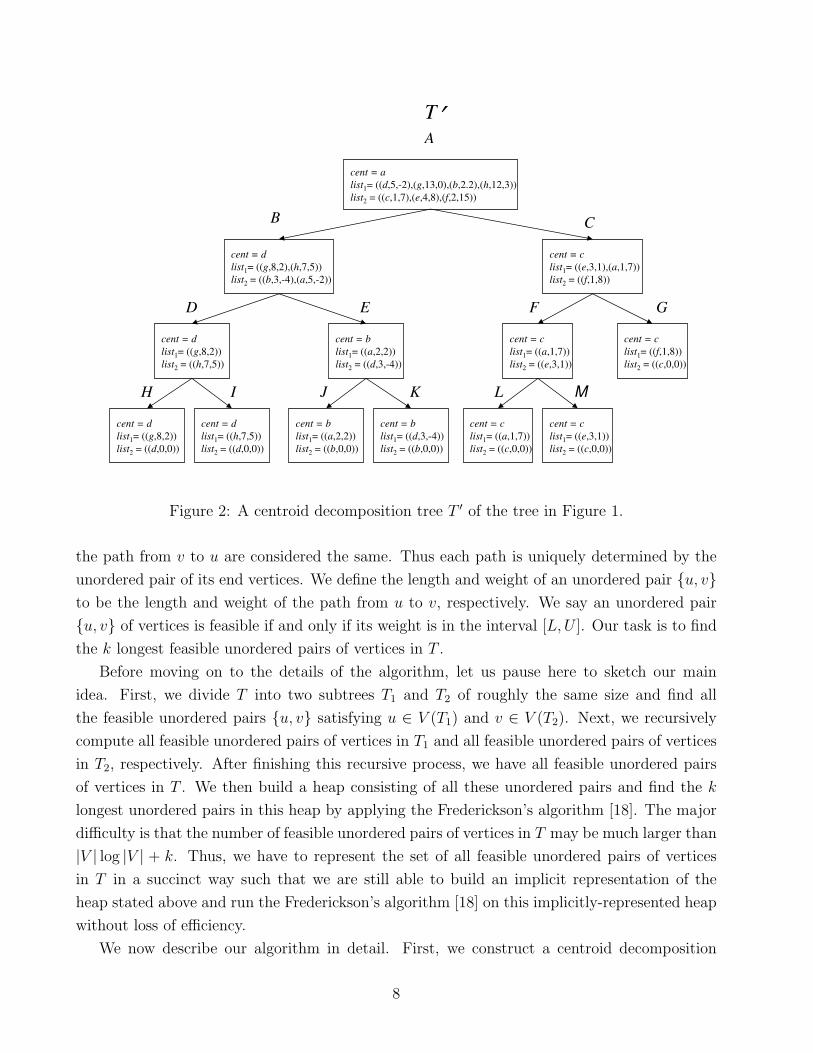
As an illustration, a tree T and its centroid decomposition tree T ′ are shown in Figure 1

and Figure 2, respectively.

Theorem 1: [Frederickson and Johnson [21]] Given a tree T (V, E) with a length function

` : E → R and a weight function w : E → R, we can construct a centroid decomposition tree

of T in O(V log V ) time.

Now we describe the Range Maxima Query (RMQ) problem. In the RMQ problem,

a list A = (a1, a2, . . . , an) of n real numbers is given to be preprocessed such that any range

maxima query can be answered quickly. A range maxima query specifies an interval [i, j] and

the goal is to find the index k with i ≤ k ≤ j such that ak achieves maximum.

We first describe a simple algorithm for solving the RMQ problem in O(n log n) preprocess-

ing time and O(1) time per query. For each 1 ≤ i ≤ n and each 1 ≤ j ≤ blog nc, we precompute

M [i][j] = arg maxk=i,...,i+2j−1ak, i.e., the index of the maximum element in A[i, i + 2j − 1].

This can be done in O(n log n) time by using dynamic programming because

M [i][j] =

M [i][j − 1] if A[M [i][j − 1]] ≥ A[M [i + 2j−1 − 1][j − 1]];

M [i + 2j−1 − 1][j − 1] otherwise.

Given a query interval [i, j], let k = blog(j − i)c. Because both [i, i + 2k − 1] and [j − 2k + 1, j]

are subintervals of [i, j] and [i, i + 2k − 1] ∪ [j − 2k + 1, j] = [i, j], the index of the maximum

element in A[i, j] is arg maxk∈M [i][i+2k−1],M [j−2k+1][j]A[k].We now sketch an algorithm for solving the RMQ problem in O(n) preprocessing time and

O(1) time per query. This algorithm was given by Bender and Farach-Coltongiven [5], and

they showed that the RMQ problem is linearly equivalent to the RMQ±1 problem which is the

same as the RMQ problem except that the adjacent elements of the input list differ by exactly

one. Thus, in the following we focus on the RMQ±1 problem. Let A = (a1, a2, . . . , an) be an

instance to the RMQ±1 problem.1 The algorithm starts by dividing the list A into 2n/ log n

1For simplicity, we assume n is a power of two.

5

shorter sublists A[1, log n2

], A[ log n2

+ 1, log n], . . . , A[n − log n2

+ 1, n], each of length log n2

. Each

sublist A[ (i−1) log n2

+ 1, i log n2

] is represented by the maximum element ri in it. They then run

the simple RMQ algorithm described in the beginning on these O(n/ log n) representatives in

O( nlog n

log( nlog n

)) = O(n) preprocessing time. By the property that adjacent elements in the

list A differs by exactly one, they use a table-lookup technique to precompute the indices of the

maximum elements in all sublists of A with lengths ≤ 2nlog n

in O(n) time. Given a query interval

[i, j], let i′ = d 2ilog n

e and j′ = b 2jlog n

c. Let rk be the maximum of ri′+1ri′+2, . . . , rj′−1, ai∗ be the

maximum element in A[i, i′ log n2

], and aj∗ be the maximum element in A[ j′ log n2

, j]. Because we

have run the simple RMQ algorithm on (r1, r2, . . . , r 2nlog n

), k can be found in constant time given

[i′+1, j′− 1]. Because both A[i, i′ log n2

] and A[ j′ log n2

, j] have lengths ≤ 2nlog n

, we can also find ai∗

and aj∗ in constant time. Note that the maximum of rk, ai∗, aj∗ is also the maximum element

in A[i, j]. Thus, if ai∗ is the maximum of rk, ai∗, aj∗, then we can directly return i∗. Similarly,

if aj∗ is the maximum of rk, ai∗, aj∗, then return j∗. Otherwise, if rk is the the maximum of

rk, ai∗, aj∗, then find and return the index of the maximum element in A[ (k−1) log n2

+ 1, k log n2

],

which can be done in constant time because A[ (k−1) log n2

+ 1, k log n2

] has length equal to 2nlog n

.

Theorem 2: [RMQ [5, 19, 25]] The RMQ problem can be solved in O(n) preprocessing time

and O(1) time per query.

For our purposes, a D-heap is a rooted degree-D tree in which each node contains a field

value, satisfying the restriction that the value of any node is larger than or equal to the values

of its children. Note that we do not require the tree to be balanced. Frederickson [18] proposed

an algorithm for finding the k largest elements in a D-heap in O(k) time. When Frederickson’s

algorithm traverses the heap to find the k largest nodes, it does not access a node unless it

has ever accessed the node’s parent. This property makes it possible to run the Frederickson’s

algorithm without first explicitly building the entire heap in the memory as long as we have a

way to obtain the information of a node given the information of its parent.

We sketch an O(k log log k)-time algorithm [18] for enumerating the k largest value nodes

in a heap as follows. For simplicity, we assume all nodes in the heap have different values. A

node is said to be of rank i if it is the ith largest node. The algorithm runs by first finding

a node u in the heap in O(k log log k) time such that the rank of u is between k and ck for

some constant c. Then the algorithm identifies all nodes in the heap not smaller than u in

O(ck) = O(k) time and returns the k largest nodes among them. To find u, we form at

most 2dk/blog kce + 1 groups of nodes, called clans. Each clan is of size at most blog kc and

represented by the smallest node in it; representatives are managed in an auxiliary heap. We

form the first clan C1 in O(log k log log k) time by grouping the largest blog kc nodes in the

original heap and initialize the auxiliary heap with the representative of C1. Set the offspring

os(C1) of C1 to the set of nodes in the original heap which are children of C1 but not in C1,

6

a

b

d f

c

e

g h

=2, w=2

=3, w=-4

=1, w=7

=8, w=2 =7, w=5

=3, w=1 =1, w=8

T

Figure 1: A tree T associated with an edge length function ` and an edge weight function w.

and set the poor relations pr(C1) of C1 to the empty set. Then for i from 1 to blog kc, do the

following. Extract the largest element in the auxiliary heap and let Cj be the clan represented

by the element extracted. If os(Cj) is not empty, then form a new clan Ci+1 in O(log k log log k)

time by grouping the blog kc largest nodes from the subheaps rooted at os(Cj) in the original

heap. Insert the representative of Ci+1 into the auxiliary heap. Set os(Ci+1) to the group of

nodes in the original heap which are children of Ci+1 but not in Ci+1, and set pr(Ci+1) to the

group of nodes which are members of os(Cj) but not included in Ci+1. If pr(Cj) is not empty,

then form a new clan Ci+2 in O(log k log log k) time by grouping the dk/blog kce largest nodes

from the subheaps rooted at pr(Cj) in the original heap. Insert the representative of Ci+2 into

the auxiliary heap. Set os(Ci+1) to the group of nodes in the original heap which are children of

Ci+2 but not in Ci+2, and set pr(Ci+2) to the group of nodes which are members of pr(Cj) but

not included in Ci+2. When the loop terminates, set u to the last element extracted from the

auxiliary heap. Since at most 2dk/blog kce + 1 clans are formed and each clan can be formed

in O(log k log log k) time, the total time is O(k log log k).

By applying the above approach recursively, plus some speed-up techniques, Frederick-

son [18] obtained an O(k)-time algorithm.

Theorem 3: [Frederickson [18]] For any constant D, we can find the k largest value nodes in

any D-heap, in O(k) time.

2.2 Finding the Weight-Constrained k Longest Paths

For simplicity, we only consider paths with at least two distinct vertices, and we do not distin-

guish between the path from u to v and the path from v to u, i.e., the path from u to v and

7

cent = a

list1= ((d,5,-2),(g,13,0),(b,2.2),(h,12,3))

list2 = ((c,1,7),(e,4,8),(f,2,15))

cent = d

list1= ((g,8,2),(h,7,5))

list2 = ((b,3,-4),(a,5,-2))

cent = c

list1= ((e,3,1),(a,1,7))

list2 = ((f,1,8))

cent = d

list1= ((g,8,2))

list2 = ((h,7,5))

cent = b

list1= ((a,2,2))

list2 = ((d,3,-4))

cent = c

list1= ((a,1,7))

list2 = ((e,3,1))

cent = c

list1= ((f,1,8))

list2 = ((c,0,0))

cent = d

list1= ((g,8,2))

list2 = ((d,0,0))

cent = d

list1= ((h,7,5))

list2 = ((d,0,0))

cent = b

list1= ((a,2,2))

list2 = ((b,0,0))

cent = b

list1= ((d,3,-4))

list2 = ((b,0,0))

cent = c

list1= ((a,1,7))

list2 = ((c,0,0))

cent = c

list1= ((e,3,1))

list2 = ((c,0,0))

A

B C

D E F G

H I J K L M

T’

Figure 2: A centroid decomposition tree T ′ of the tree in Figure 1.

the path from v to u are considered the same. Thus each path is uniquely determined by the

unordered pair of its end vertices. We define the length and weight of an unordered pair u, vto be the length and weight of the path from u to v, respectively. We say an unordered pair

u, v of vertices is feasible if and only if its weight is in the interval [L,U ]. Our task is to find

the k longest feasible unordered pairs of vertices in T .

Before moving on to the details of the algorithm, let us pause here to sketch our main

idea. First, we divide T into two subtrees T1 and T2 of roughly the same size and find all

the feasible unordered pairs u, v satisfying u ∈ V (T1) and v ∈ V (T2). Next, we recursively

compute all feasible unordered pairs of vertices in T1 and all feasible unordered pairs of vertices

in T2, respectively. After finishing this recursive process, we have all feasible unordered pairs

of vertices in T . We then build a heap consisting of all these unordered pairs and find the k

longest unordered pairs in this heap by applying the Frederickson’s algorithm [18]. The major

difficulty is that the number of feasible unordered pairs of vertices in T may be much larger than

|V | log |V | + k. Thus, we have to represent the set of all feasible unordered pairs of vertices

in T in a succinct way such that we are still able to build an implicit representation of the

heap stated above and run the Frederickson’s algorithm [18] on this implicitly-represented heap

without loss of efficiency.

We now describe our algorithm in detail. First, we construct a centroid decomposition

8

tree T ′ = (V ′, E ′, r) of T in O(V log V ) time by Theorem 1. For each v ∈ V ′ and i ∈ 1, 2,let (vi,j, `(v.cent, vi,j), w(v.cent, vi,j)) be the jth element of v.listi if it exists. Note that since∑

v∈V ′(|v.list1|+ |v.list2|+1) = O(V log V ), we can find `(v.cent, vi,j) and w(v.cent, vi,j) for all

v ∈ V ′, i ∈ 1, 2 and 1 ≤ j ≤ |v.listi| in total O(V log V ) time. By the next lemma, in total

O(V log V ) time, for all v ∈ V ′ and 1 ≤ i ≤ |v.list1|, we can find an interval [pvi , q

vi ] such that

1. w(v.cent, v1,i) + w(v.cent, v2,j) = w(v1,i, v2,j) ∈ [L,U ] for all j ∈ [pvi , q

vi ];

2. w(v1,i, v2,j) 6∈ [L,U ] for all j 6∈ [pvi , q

vi ].

It follows that the set of all feasible unordered pairs of vertices in T is equal to the set⋃v∈V ′

⋃|v.list1|i=1 v1,i, v2,j : j ∈ [pv

i , qvi ].

Lemma 1: Let T ′ = (V ′, E ′, r) be a centroid decomposition tree of T = (V, E). In total

O(V log V ) time, for all v ∈ V ′ and 1 ≤ i ≤ |v.list1|, we can find an interval [pvi , q

vi ] such that

(1) w(v1,i, v2,j) ∈ [L,U ] for all j ∈ [pvi , q

vi ] and (2) w(v1,i, v2,j) 6∈ [L, U ] for all j 6∈ [pv

i , qvi ].

Proof: Since∑

v∈V ′(|v.list1|+ |v.list2|+ 1) = O(V log V ), we only have to show that for each

v ∈ V ′, we can compute [pvi , q

vi ] for all 1 ≤ i ≤ |v.list1| in total O(|v.list1|+ |v.list2|+ 1) time.

Given v ∈ V ′, we claim the following procedure computes [pvi , q

vi ] for all 1 ≤ i ≤ |v.list1| in

total O(|v.list1|+ |v.list2|+ 1) time.

1. Let n′ = |v.list1| and m′ = |v.list2|.

2. If n′ = 0 or m′ = 0 then stop.

3. Set p and q to m′.

4. For i ← 1 to n′ do

(a) While(w(v1,i, v2,p−1) ≥ L and p− 1 ≥ 1) do p ← p− 1.

(b) While(w(v1,i, v2,q) > U and q ≥ p) do q ← q − 1.

(c) pvi ← p and qv

i ← q.

It is not hard to see the running time of this procedure is O(|v.list1| + |v.list2| + 1) since

both the values of p and q are nonincreasing. To verify the correctness, it suffices to note that

since the list v.listi, i ∈ 1, 2, is sorted on w(v.cent, vi,j), the sequence (pv1, . . . , p

v|v.list1|) and

the sequence (qv1 , . . . , q

v|v.list1|) must be nonincreasing.

Next, for each v ∈ V ′, we preprocess v.list2 so that given any interval [i, j], we can find the

index k, denoted RMQ(v.list2, i, j), in [i, j] such that `(v.cent, v2,k) achieves maximum in O(1)

time. By Theorem 2, this preprocessing can be done in O(∑

v∈V ′ |v.list2|) = O(V log V ) time.

9

Before going on to the next point, we would like to define some data structures. For each

v ∈ V ′ and 1 ≤ i ≤ |v.list1|, define H(v1,i) to be a rooted ordered binary tree which consists of

nodes with fields pair, value, and interval and satisfies the following properties.

1. There are total |v.list1| nodes in H(v1,i) and the interval of the root of H(v1,i) is [pvi , q

vi ].

2. For each node u of H(v1,i), if p < k then u’s left child has interval [p, k − 1], and

if k < q then u’s right child has interval [k + 1, q], where [p, q] = u.interval and

k =RMQ(v.list2, p, q).

3. For each node u of H(v1,i), if u.interval = [p, q] then u.pair = v1,i, v2,k and u.value =

`(v1,i, v2,k), where k =RMQ(v.list2, p, q).

Let us now return to describe our algorithm. Denote by V (H(v1,i)) the set of nodes in

H(v1,i). It should be noticed that the set of all feasible unordered pairs of vertices in T is equal

to the set

⋃

v∈V ′

|v.list1|⋃i=1

v1,i, v2,j : j ∈ [pvi , q

vi ] =

⋃

v∈V ′

|v.list1|⋃i=1

u.pair : u ∈ V (H(vi)).

Therefore, the remaining work is to find the k largest value nodes in⋃

v∈V ′⋃|v.list1|

i=1 V (H(v1,i)).

Clearly, we can not afford to construct H(v1,i) explicitly for each v1,i. But notice that given

any node u of H(v1,i), we can always construct u’s children in O(1) time since we have done the

RMQ preprocessing on the list v.list2. Thus we shall only construct the root of H(v1,i) in the

first instance and expand the tree as needed. Since we have known pvi and qv

i for each v ∈ V ′

and 1 ≤ i ≤ |v.list1| and done the RMQ preprocessing on the list v.list2 for each v ∈ V ′, we

can construct, in total O(V log V ) time, the root of H(v1,i) for all v1,i. Then we place these

roots into a balanced 2-heap of size up to O(V log V ) by the heapify operation [15] in linear

time, i.e., in O(V log V ) time. Note that each H(v1,i) is a 2-heap, so we have conceptually built

a 4-heap for the set⋃

v∈V ′⋃|v.list1|

i=1 V (H(v1,i)). Now by Theorem 3, we can apply Frederickson’s

algorithm [18] to find the k largest value nodes in that 4-heap in O(k) time. Of course, except

the roots of all H(v1,i), all the nodes in that 4-heap are not physically created until they are

needed in running Frederickson’s [18] algorithm. We summarize the results of this section by

the following theorem.

Theorem 4: Let T = (V, E) be a tree with a length function ` : E → R and a weight function

w : E → R. Given T , a positive integer k and an interval [L,U ], we can find the k longest

paths among all paths in T with weights in the interval [L,U ] in O(V log V + k) time.

10

3 Ω(V log V +k) Lower Bound for the Weight-Constrained

k Longest Paths Problem

We prove that the Weight-Constrained Longest Path problem has an Ω(V log V ) bound

in the algebraic computation tree model. It follows that the Weight-Constrained k Longest

Paths problem has an Ω(V log V + k) lower bound in the algebraic computation tree model

since extra Ω(k) time is necessary for outputting the answer.

Definition 4: [Set Intersection Problem] Given two sets x1, x2, . . . , xn and y1, y2, . . . , yn,the Set Intersection problem asks whether there exist indices i and j such that xi = yj.

Lemma 2: [Ben-Or [8]] The Set Intersection problem has an Ω(n log n) lower bound in

the algebraic computation tree model.

Theorem 5: The Weight-Constrained Longest Path problem has an Ω(V log V ) lower

bound in the algebraic computation tree model.

Proof: We reduce the Set Intersection problem to the Weight-Constrained Longest

Path problem. Given two sets x1, x2, . . . , xn and y1, y2, . . . , yn, we construct, in O(n)

time, a problem instance of the Weight-Constrained Longest Path problem as follows.

We first construct a tree T = (V, E), where V = x′1, . . . , x′n ∪ y′1, . . . , y′n ∪ c1, c2 and

E = x′1c1, . . . , x′nc1 ∪ y′1c2, . . . , y′nc2 ∪ c1c2. Define the length function ` : E → R by

letting `(e) = 1 for all e ∈ E. Define the weight function w : E → R by letting w(x′ic1) = xi

and w(y′ic2) = −yi for all i = 1, . . . , n, and w(c1c2) = 0. Set both the weight lower bound L

and the weight upper bound U of paths to 0. It can be verified that the longest path in T with

weight = 0 has length 3 if and only if there exist indices i and j such that xi = yj. Since in this

reduction we have |V | = 2n + 2 and the Set Intersection problem has an Ω(n log n) in the

algebraic computation tree model by Lemma 2, we conclude that the Weight-Constrained

Longest Path problem has an Ω(V log V ) lower bound in the algebraic computation tree

model.

Corollary 1: The Weight-Constrained k Longest Paths problem has an Ω(V log V +k)

lower bound in the algebraic computation tree model.

4 O(n + k)-time Algorithm for the Length-Constrained k

Maximum-Sum Segments Problem

Given a sequence A = (a1, a2, . . . , an) of numbers, we define the sum and length of a segment

A[i, j] to be ai + ai+1 + · · · + aj and j − i + 1, respectively. The Length-Constrained

11

k Maximum-Sum Segments problem is to find the k maximum-sum segments among all

segments with lengths in a specified interval [L, U ]. In the following, we show how to solve the

Length-Constrained k Maximum-Sum Segments problem in O(n + k) time.

4.1 Preliminaries

Let P denote the prefix-sum array of the input sequence A, i.e., P [0] = 0 and P [i] = a1 + a2 +

· · ·+ai for i = 1, . . . , n. P can be computed in linear time by set P [0] to 0 and P [i] to P [i−1]+ai

for i = 1, 2, . . . , n. Let S[i, j] denote the sum of A[i, j]. Since S[i, j]=P [j]− P [i − 1], the sum

of any segment can be computed in constant time after the prefix-sum array is constructed.

Now we describe the Range Maximum-Sum Segment Query (RMSQ) problem. In the

RMSQ problem, a sequence A = (a1, a2, . . . , an) of n numbers is given to be preprocessed such

that any range maximum-sum segment query can be answered quickly. A range maximum-sum

segment query specifies two intervals [i, j] and [k, l], and the goal is to find a pair of indices

(x, y) with i 6 x 6 j and k 6 y 6 ` that maximizes S[x, y].

Chen and Chao [11] have showed that RMSQ is linearly equivalent to RMQ. For ease of

explanation, in the following description of the algorithm we use RMSQ instead of RMQ.

Theorem 6: [Chen and Chao [11]] The RMSQ problem can be solved in O(n) preprocessing

time and O(1) time per query.

4.2 Finding the Length-Constrained k Maximum-Sum Segments

The algorithm is similar to the one in Section 2.2, but this time we can achieve linear running

time. First we preprocess the input sequence A so that given any two intervals [i, j] and [k, l], we

can find the pair (x, y), denoted RMSQ(i, j, k, l), with i 6 x 6 j and k 6 y 6 ` that maximizes

S[x, y]. By Theorem 6, this preprocessing can be done in O(n) time. In the following, we say

a segment A[i, j] is feasible if and only if L ≤ j − i + 1 ≤ U . Set pi = maxi − U + 1, 1and qi = i − L + 1 for all i = 1, . . . , n. For simplicity, we assume pi ≤ qi for all i = 1, . . . , n.

Then⋃n

i=1A[h, i] : h ∈ [pi, qi] is the set of all feasible segments. Our task is to find the k

maximum-sum segments in this set.

Before moving on to the algorithm, let us define some data structures. For each index i,

define H(i) to be a rooted ordered binary tree which consists of nodes with fields pair, value,

and interval and satisfies the following properties.

1. There are total qi − pi + 1 nodes in H(i) and the interval of the root of H(i) is [pi, qi].

2. For each node u of H(i), if p < k then u’s left child has interval [p, k−1], and if k < q then

u’s right child has interval [k+1, q], where [p, q] = u.interval and (k, i) =RMSQ(p, q, i, i).

12

3. For each node u of H(i), if u.interval = [p, q] then u.pair = (k, i) and u.value = S[k, i],

where (k, i)=RMSQ(p, q, i, i).

We now describe our algorithm. Let V (H(i)) denote the set of nodes in H(i). It is clear that

the k largest value nodes in⋃n

i=1 V (H(i)) correspond to the k maximum-sum feasible segments.

Thus the remaining work is to find the k largest value nodes in⋃n

i=1 V (H(i)). Notice that given

any node u of H(i), we can always construct u’s children in O(1) time since we have done the

RMSQ preprocessing on A[1..n]. Thus we only construct the root of H(i) in the first instance

and expand the tree as needed. Since we have known pi and qi for each index i and done the

RMSQ preprocessing on A[1..n], we can construct, in total O(n) time, the root of H(i) for

each index i. Then we place these roots into a balanced 2-heap by the heapify operation [15]

in O(n) time. Note that each H(i) is a 2-heap, so we have conceptually built a 4-heap for the

set⋃n

i=1 V (H(i)). Now by Theorem 3, we can apply Frederickson’s algorithm [18] to find the k

largest value nodes in that 4-heap in O(k) time. As before, except the roots of all H(i), all the

nodes in that 4-heap are not physically created until they are needed in running Frederickson’s

[18] algorithm. The following theorem summarizes the results of this section.

Theorem 7: Given a sequence A = (a1, . . . , an) of numbers, a positive integer k, and an

interval [L,U ], we can find, in O(n + k) time, the k maximum-sum segments of A with lengths

in [L, U ].

Definition 5: Let A = ((a1, `1), . . . , (an, `n)) be a sequence of pairs of numbers, where `i > 0

for all i = 1, . . . , n. We define the sum, length, and density of a segment A[i, j] to be∑

i≤h≤j ah,∑i≤h≤j `h, and

Pi≤h≤j ahPi≤h≤j `h

, respectively.

We prove the following stronger theorem by slightly modifying the above algorithm.

Theorem 8: Given a sequence of pairs of numbers A = ((a1, `1), . . . , (an, `n)), where `i > 0

for i = 1, . . . , n, a positive integer k, and an interval [L,U ], we can find, in O(n + k) time, the

k maximum-sum segments of A with lengths in [L,U ].

Proof: We show how to modify the above algorithm to achieve this theorem. In fact, we

only need to change the settings of pi’s and qi’s. The remaining parts are the same. For all

i = 1, . . . , n, we redefine pi to be the minimum index 1 ≤ h ≤ i such that £[h, i] ≤ U and qi to

be the maximum index 1 ≤ h′ ≤ i such that £[h′, i] ≥ L. For simplicity, we assume pi and qi

exist for all i = 1, . . . , n. Since `i is positive for all i = 1, . . . , n, the sequences (p1, . . . , pn) and

(q1, . . . , qn) must be nondecreasing. Thus we can compute pi and qi for all i = 1, . . . , n by the

following procedure in O(n) time.

1. Set p = 1 and q = 1.

13

2. For i ← 1 to n do

(a) While(£[p, i] > U and p ≤ i) do p ← p + 1.

(b) While(£[q + 1, i] ≥ L and q + 1 ≤ i) do q ← q + 1.

(c) pi ← p and qi ← q.

3. Output (p1, . . . , pn) and (q1, . . . , qn).

5 Applications

In this section, we give some applications of our algorithms.

5.1 Finding the Weight-Constrained k Largest Elements of X + Y

Let X and Y be two sets associated with value functions VX : X → R and VY : Y → R,

respectively. The Cartesian sum X + Y is the set (x, y) : (x, y) ∈ X × Y associated with a

value function V : X×Y → R defined by letting V (x, y) = VX(x)+VY (y) for all (x, y) ∈ X×Y .

For convenience, we just use x + y to denote VX(x) + VY (y), and we call a set associated with

a value function a valued set. Frederickson and Johnson [20] gave an optimal algorithm for

finding the kth largest element in X + Y in O(m + p log(k/p)) time, where m = |X| ≤ |Y | = n

and p = mink,m. Recently Bae and Takaoka proposed an efficient O(n + k log k)-time

algorithm [4] for finding the k largest elements of X + Y . In the following, we first show how

to find the k largest elements of X + Y in O(n + k) time by using Eppstein’s algorithm [16],

and then we show how to cope with the weight-constrained case in O(n log n+k) time by using

our algorithm.

Lemma 3: [Eppstein [16]] Given a directed acyclic graph G = (V, E) with a length function

` : E → R and two distinguished vertices s and t, we can find, in O(V + E + k) time, an

implicit representation of the k longest paths connecting s and t in G. And by using the

implicit representation, we can list the edges of any path P in the set of the k longest paths in

time proportional to the number of edges in P .

Theorem 9: Given two valued sets X = x1, . . . , xn and Y = y1, . . . , yn, we can find the

k largest elements of X + Y in O(n + k) time.

14

Proof: We describe an O(n + k) algorithm for finding the k largest elements of X + Y as

follows. We first construct, in O(n) time, a directed acyclic graph G = (V, E) where V =

s, t, c∪x′1, . . . , x′n∪y′1, . . . , y′n and E = −→sx′1, . . . ,−→sx′n∪

−→x′1c, . . . ,

−→x′nc∪

−→cy′1, . . . ,

−→cy′n∪

−→y′1t, . . . ,−→y′nt. Define ` : E → R by letting `(

−→sx′i) = 0, `(

−→x′ic) = xi, `(

−→cy′i) = yi, and `(

−→x′it) = 0

for all i = 1, . . . , n. It can be verified that (xi, yj) is the kth largest element of X + Y if and

only if (s, x′i, c, y′j, t) is the kth longest path connecting s and t in G. Thus, by Lemma 3, we

can first find the k longest paths connecting s and t in G in O(V + E + k) = O(n + k) time

and then find the corresponding k largest elements of X + Y in O(k) time.

Now we show how to cope with the weight-constrained case. Let X and Y be two valued

sets associated with weight functions WX : X → R and WY : Y → R, respectively. Then for

each (x, y) ∈ X + Y , we define the weight of (x, y) to be WX(x) + WY (y).

Theorem 10: Let X = x1, . . . , xn and Y = y1, . . . , yn be two valued sets associated with

weight functions WX : X → R and WY : Y → R, respectively. Given a positive integer k and

an interval [L,U ], we can find, in O(n log n + k) time, the k largest elements of X + Y with

weights in the interval [L,U ].

Proof: We construct, in O(n) time, a tree T = (V, E) where V = x′1, . . . , x′n∪ y′1, . . . , y′n∪c and E = x′1c, . . . , x′nc ∪ y′1c, . . . , y′nc. Let δ be a large enough positive number, say,

greater than max|U |, |L| + maxmax1≤i≤n

|WX(xi)|, max1≤i≤n

|WY (yi)|. Define the weight function

w : E → R by letting w(x′ic) = WX(xi) + δ and w(y′ic) = WY (yi) − δ for all i = 1, . . . , n.

Define the length function ` : E → R by letting `(x′ic) = VX(xi) and `(y′ic) = VY (yi) for all

i = 1, . . . , n.

Let P be a path of T . Consider the following cases. First, if P has both of its end vertices in

x′1, . . . , x′n, i.e., P = (x′i, c, x′j) for some i and j, then we have w(P ) = WX(xi)+WX(xj)+2δ >

U . Second, if P has one end vertex in x′1, . . . , x′n and the other end vertex being c, i.e.,

P = (x′i, c) for some i, then we also have w(P ) = WX(xi) + δ > U . Similarly, if P has both of

its end vertices in y′1, . . . , y′n or P has one end vertex in y′1, . . . , y′n and the other end vertex

being c, then we have w(P ) < L. Finally, if P has one end vertex in x′1, . . . , x′n and the other

in y′1, . . . , y′n, i.e., P = (x′i, c, y′j) for some i and j, then we have w(P ) = WX(xi) + WY (yj)

and v(P ) = VX(xi) + VY (yj).

From the above discussion, we conclude that (xi, yj) is the kth largest element of X + Y

with weight in [L,U ] if and only if (x′i, c, y′j) is the kth longest path of T with weight in [L,U ].

Thus, by Theorem 4, we can first find the k longest paths of T with weights in [L,U ] in

O(V log V + k) = O(n log n + k) time and then find the corresponding k largest elements of

X + Y with weights in [L,U ] in O(k) time.

15

5.2 Finding the Sum-Constrained k Longest Segments

In biological sequence analysis, several researchers have devoted to the problem of finding the

longest segment whose sum is not less than a specified lower bound L [1, 12, 35]. Allison [1]

gave an algorithm which runs in linear time if the input sequence is a 0-1 sequence and L is

a rational number. For real number sequences and real number lower bound, Wang and Xu

[35] provided the first linear time algorithm, and Chen and Chao [12] gave an alternative linear

time algorithm which runs in an online manner. We consider a more general problem in which

both the lower bound L and the upper bound U of the sums of the segments are given and we

want to find the k longest segments whose sums satisfy both the lower bound condition and

the upper bound condition.

Theorem 11: Given a sequence A = (a1, a2, . . . , an) of real numbers and an interval [L,U ],

we can find, in O(n log n+k) time, the k longest segments whose sums are in the interval [L,U ].

Proof: Directly from Theorem 4.

5.3 Finding k Length-Constrained Maximum-Density Segments Sat-

isfying a Density Lower Bound

Given a sequence of pairs of numbers A = ((a1, `1), . . . , (an, `n)), where `i > 0 for all i = 1, . . . , n,

a positive integer k, an interval [L,U ], and a number δ, let kout = mink, nδ, where nδ is the

total number of segments of A with lengths in [L,U ] and densities ≥ δ. We show how to find kout

segments of A with lengths in [L,U ] and densities ≥ δ in O(n+ kout) time. A segment A[i, j] is

called a feasible segment if and only if the length of A[i, j] is in [L,U ]. Let δmax be the density

of the feasible segment which has the maximum density among all feasible segments. The

Length-Constrained Maximum-Density Segment problem is to find a feasible segment

with density equal to δmax. The Length-Constrained Maximum-Density Segment

problem is well studied in [14, 24, 26, 27, 29, 30] and can be solved in linear time by [14, 24].

Let nδmax be the total number of feasible segments with density equal to δmax. If we are

not satisfied by finding only one feasible segments with density equal to δmax, then by first

computing δmax by O(n)-time algorithms in [14, 24] and setting δ to δmax, our algorithm can

list kout = mink, nδmax feasible segments with density equal to δmax in O(n + kout) time.

Theorem 12: Given a sequence of pairs of numbers A = ((a1, `1), . . . , (an, `n)), where `i > 0

for all i = 1, . . . , n, a positive integer k, an interval [L,U ], and a number δ, let kout = mink, nδ,where nδ is the total number of segments of A with lengths in [L,U ] and densities ≥ δ. Then

we can find, in O(n + kout) time, kout segments of A with lengths in [L,U ] and densities ≥ δ.

16

Proof: In the following, a segment is called a feasible segment if and only if its length is

in [L, U ]. Let A′ = ((a1 − `1δ, `1), (a2 − `2δ, `2), . . . , (an − `nδ, `n)). Since A[i, j] has densityai+···+aj

`i+···+`j≥ δ if and only if A′[i, j] has sum

∑i≤h≤j(ah− `hδ) ≥ 0, it suffices to show how to find

kout feasible segments of A′ with sums ≥ 0 in O(n + kout) time. As in the proof of Theorems 7

and 8, we first implicitly construct a heap for all feasible segments of A′ in O(n) time. Let

2t−1 ≤ k < 2t. We then execute the following procedure to find kout feasible segments of A′

with sums ≥ 0 in O(kout + 1) time, so the total time is O(n + kout).

1. For i ← 0 to t do

(a) S ← the 2i maximum-sum feasible segments of A′.

(b) If some segment in S has sum less than 0, then stop the loop.

2. If S contains more than k segments with sums ≥ 0, then return k of them; otherwise,

return all segments in S with sums ≥ 0.

We now prove that the procedure runs in O(kout + 1) time. By Theorem 3, the ith iteration

of the loop in Step 1 can be done in O(2i) time. If nδ = 0, then it is clear that this procedure

returns in constant time; otherwise, there are two cases to consider.

Case 1: nδ ≥ k. In this case, the loop continues until the tth iteration, so the total time

spent on Step 1 is O(1 + 2 + 4 + · · ·+ 2t) = O(2t+1) = O(k) = O(mink, nδ) = O(kout). After

the loop stops, the size of S is at most 2t, so Step 2 can also be done in O(2t) = O(k) =

O(mink, nδ) = O(kout) time.

Case 2: nδ < k. Let 2t−1 ≤ nδ < 2t. In this case, the loop continues until the tth it-

eration, so the total time spent on Step 1 is O(1 + 2 + 4 + · · · + 2t) = O(2t+1) = O(nδ) =

O(mink, nδ) = O(kout). After the loop stops, the size of S is at most 2t, so Step 2 can also

be done in O(2t) = O(nδ) = O(mink, nδ) = O(kout) time.

5.4 Finding the Area-Constrained k Maximum-Sum Subarrays

Given an n × n array A[1..n][1..n], define the sum and area of a subarray A[k..l][i..j] to be∑lp=k

∑jq=i A[p][q] and (l− k + 1)(j − i + 1), respectively. The k Maximum-Sum Subarrays

problem is well studied in [2, 3, 4, 6, 10, 13, 31, 32] and can be solved in O(n3 + k) time by

Brodal and Jørgensen [10] and O(n3 ·√

log log nlog n

+ k log n) time by Bae and Takaoka [4].

In the following, we prove that the Area-Constrained k Maximum-Sum Subarrays

problem can be solved in O(n3 + k) time by applying Theorem 8.

Theorem 13: Given an n × n array A[1..n][1..n] and an interval [L,U ], we can find, in

O(n3 + k) time, the k maximum-sum subarrays with areas in [L,U ].

17

Proof: First we have to construct strips Si,j = ((∑

i≤h≤j A[h][1], j− i+1), (∑

i≤h≤j A[h][2], j−i + 1), . . . , (

∑i≤h≤j A[h][n], j − i + 1)) for all 1 ≤ i ≤ j ≤ n in O(n3) time. Then we construct

a sequence S by concatenating these strips with pairs (0, U + 1). Noting that pairs (0, U + 1)

play the role of a stopper, it is not hard to see that each segment of S with length in [L, U ]

corresponds to a subarray of A with area in [L,U ], and vice versa. Thus we can first apply

Theorem 8 to find k maximum-sum segments of S with lengths in [L,U ] in O(n3 + k) time and

then output their corresponding subarrays of A.

6 Concluding Remarks

In this work, we show how to efficiently enumerate all the weight-constrained k longest paths

in a tree and all the length-constrained k maximum-sum segments of a sequence. In the future,

it will be interesting to consider problems like selecting the weight-constrained kth longest path

in a tree and the length-constrained kth largest sum segment of a sequence.

Acknowledgments

We thank the anonymous referees for their thoughtful reading of the manuscript and many

helpful suggestions. We thank Gerth S. Brodal, Kuan-Yu Chen, Allan G. Jørgensen, and

Hung-Lung Wang for helpful comments.

References

[1] Lloyd Allison. Longest Biased Interval and Longest Non-Negative Sum Interval. Bioinfor-

matics, 19(10):1294–1295, 2003.

[2] Sung Eun Bae and Tadao Takaoka. Algorithms for the Problem of k Maximum Sums

and a VLSI Algorithm for the k Maximum Subarrays Problem. In Proceedings of the 7th

International Symposium on Parallel Architectures, Algorithms and Networks, 247–253,

2004.

[3] Sung Eun Bae and Tadao Takaoka. Improved Algorithms for the k-Maximum Subarray

Problem for Small k. In Proceedings of the 11th Annual International Computing and

Combinatorics Conference, 621–631, 2005.

18

[4] Sung Eun Bae and Tadao Takaoka. A Sub-Cubic Time Algorithm for the k-Maximum Sub-

array Problem. In Proceedings of the 18th Annual International Symposium on Algorithms

and Computation, 751–762, 2007.

[5] Michale A. Bender and Martin Farach-Colton. The LCA Problem Revisited. In Proceedings

of the 4th Latin American Symposium on Theoretical Informatics, 88–94, 2000.

[6] Fredrik Bengtsson and Jingsen Chen. Efficient Algorithms for k Maximum Sums. In Pro-

ceedings of the 15th Annual International Symposium on Algorithms and Computation,

137–148, 2004.

[7] Jon Bentley. Programming Pearls: Algorithm Design Techniques. Communications of the

ACM, 865–871, 1984.

[8] Michael Ben-Or. Lower Bounds for Algebraic Computation Trees. In Proceedings of the

15th Annual ACM Symposium on Theory of Computing, 80–86, 1983.

[9] Manuel Blum, Robert W. Floyd, Vaughan Pratt, Ronald L. Rivest, and Robert E. Tarjan.

Time Bounds for Selection. Journal of Computer and System Sciences, 7(4):448–461, 1973.

[10] Gerth S. Brodal and Allan G. Jørgensen. A Linear Time Algorithm for the k Maximal Sums

Problem. In Proceedings of the 32nd International Symposium on Mathematical Founda-

tions of Computer Science, 442–453, 2007.

[11] Kuan-Yu Chen and Kun-Mao Chao. On the Range Maximum-Sum Segment Query Prob-

lem. Discrete Applied Mathematics, 155(16):2043–2052, 2007.

[12] Kuan-Yu Chen and Kun-Mao Chao. Optimal Algorithms for Locating the Longest and

Shortest Segments Satisfying a Sum or an Average Constraint. Information Processing

Letters, 96(6):197–201, 2005.

[13] Chih-Huai Cheng, Kuan-Yu Chen, Wen-Chin Tien and Kun-Mao Chao. Improved Algo-

rithms for the k Maximum-Sums Problems. Theoretical Computer Science, 362(13):162–

170, 2006.

[14] Kai-Min Chung and Hsueh-I Lu. An Optimal Algorithm for the Maximum-Density Seg-

ment Problem. SIAM Journal on Computing, 34(2):373-387, 2004.

[15] Thomas H. Cormen, Charles E. Leiserson, Ronald L. Rivest, and Clifford Stein. Introduc-

tion to Algorithms. The MIT Press, second edition, 2001.

[16] David Eppstein. Finding the k Shortest Paths. SIAM Journal on Computing, 28(2):652–

673,1998.

19

[17] Tsai-Hung Fan, Shufen Lee, Hsueh-I Lu, Tsung-Shan Tsou, Tsai-Cheng Wang, and Adam

Yao. An Optimal Algorithm for Maximum-Sum Segment and Its Application in Bioinfor-

matics Extended Abstract. In Proceeding of the 8th International Conference on Imple-

mentation and Application of Automata: 251-257, 2003.

[18] Greg N. Frederickson. An Optimal Algorithm for Selection in a Min-Heap. Information

and Computation 104(2):197–214, 1993.

[19] Johannes Fischer and Volker Heun. Theoretical and Practical Improvements on the RMQ-

Problem, with Applications to LCA and LCE. In Proceedings of the 17th Annual Sympo-

sium on Combinatorial Pattern Matching, 36–48, 2006.

[20] Greg N. Frederickson and Donald B. Johnson. The Complexity of Selection and Ranking

in X + Y and Matrices with Sorted Rows and Columns. Journal of Computer and System

Science, 24(2):197–208, 1982.

[21] Greg N. Frederickson and Donald B. Johnson. Finding kth paths and p-Centers by Gen-

erating and Searching Good Data Structures. Journal of Algorithms, 4(1):61–80, 1983.

[22] Takeshi Fukuda, Yasuhiko Morimoto, Shinichi Morishita, and Takeshi Tokuyama: Data

Mining with Optimized Two-Dimensional Association Rules. ACM Transactions on

Database Systems, 26(2):179–213, 2001.

[23] Ulf Grenander. Pattern Analysis. Springer-Verlag, New York, 1978.

[24] Michael Goldwasser, Ming-Yang Kao and Hsueh-I Lu. Linear-Time Algorithms for Com-

puting Maximum-Density Sequence Segments with Bioinformatics Applications. Journal

of Computer and System Sciences, 70(2):128–144, 2005.

[25] Dov Harel and Robert E. Tarjan. Fast Algorithms for Finding Nearest Common Ancestors.

SIAM Journal on Computing, 13(2):338–355, 1984.

[26] Xiaoqiu Huang. An Algorithm for Identifying Regions of a DNA Sequence that Satisfy a

Content Requirement. Computer Applications in the Biosciences, 10:219–225, 1994.

[27] Sung Kwon Kim. Linear-Time Algorithm for Finding a Maximum-Density Segment of a

Sequence. Information Processing Letters, 86(6):339–342, 2003.

[28] Sung Kwon Kim. Finding a Longest Nonnegative Path in a Constant Degree Tree. Infor-

mation Processing Letters, 93(6):275–279, 2003.

[29] Yaw-Ling Lin, Xiaoqiu Huang, Tao Jiang and Kun-Mao Chao. MAVG: Locating Non-

Overlapping Maximum Average Segments in a Given Sequence. Bioinformatics, 19(1):151–

152, 2003.

20

[30] Yaw-Ling Lin, Tao Jiang and Kun-Mao Chao. Efficient Algorithms for Locating the

Length-Constrained Heaviest Segments with Applications to Biomolecular Sequence Anal-

ysis. Journal of Computer and System Sciences, 65(3):570–586, 2002.

[31] Tien-Ching Lin and D. T. Lee. Randomized Algorithm for the Sum Selection Problem. In

Proceedings of the 16th Annual International Symposium on Algorithms and Computation,

515–523, 2005.

[32] Tien-Ching Lin and D. T. Lee. Efficient Algorithm for the Sum Selection Problem and k

Maximum Sums Problem. In Proceedings of the 17th Annual International Symposium on

Algorithms and Computation, 460–473, 2006.

[33] Nimrod Megiddo, Arie Tamir, Eitan Zemel, and Ramaswamy Chandrasekaran. An

O(n log2 n) Algorithm for the kth Longest Path in a Tree with Applications to Location

Problems. SIAM Journal on Computing, 10(2):328–337, 1981.

[34] Kalyan Perumalla and Narsingh Deo. Parallel Algorithms for Maximum Subsequence and

Maximum Subarray. Parallel Processing Letters, 5:367–373, 1995.

[35] Lusheng Wang and Ying Xu. SEGID: Identifying Interesting Segments in (Multiple) Se-

quence Alignments. Bioinformatics, 19(2):297–298, 2003.

[36] Bang Ye Wu, Kun-Mao Chao, and Chuan Yi Tang. An Efficient Algorithm for the Length-

Constrained Heaviest Path Problem on a Tree. Information Processing Letters, 69(2):63–

67, 1999.

[37] Bang Ye Wu and Kun-Mao Chao. Spanning Trees and Optimization Problems. Chap-

man & Hall/CRC, first edition, 2004.

21