Repetition-free longest common subsequence of random sequences

Cristina G. Fernandes ∗ Marcos Kiwi †

May 22, 2013

Abstract

A repetition free Longest Common Subsequence (LCS) of two sequences x and y is an LCS of x and ywhere each symbol may appear at most once. Let R denote the length of a repetition free LCS of twosequences of n symbols each one chosen randomly, uniformly, and independently over a k-ary alphabet.We study the asymptotic, in n and k, behavior of R and establish that there are three distinct regimes,depending on the relative speed of growth of n and k. For each regime we establish the limiting behaviorof R. In fact, we do more, since we actually establish tail bounds for large deviations of R from itslimiting behavior.

Our study is motivated by the so called exemplar model proposed by Sankoff (1999) and the relatedsimilarity measure introduced by Adi et al. (2007). A natural question that arises in this context, whichas we show is related to long standing open problems in the area of probabilistic combinatorics, is tounderstand the asymptotic, in n and k, behavior of parameter R.

1 Introduction

Several of the genome similarity measures considered in the literature either assume that the genomes do notcontain gene duplicates, or work efficiently only under this assumption. However, several known genomes docontain a significant amount of duplicates. (See the review on gene and genome duplication by Sankoff [17]for specific information and references.) One can find in the literature proposals to address this issue.Some of these proposals suggest to filter the genomes, throwing away part or all of the duplicates, andthen applying the desired similarity measure to the filtered genomes. (See [2] for a description of differentsimilarity measures and filtering models for addressing duplicates.)

Sankoff [16], trying to take into account gene duplication in genome rearrangement, proposed the so calledexemplar model, which is one of the filtering schemes mentioned above. In this model, one searches, for eachfamily of duplicated genes, an exemplar representative in each genome. Once the representative genes areselected, the other genes are disregarded, and the part of the genomes with only the representative genes issubmitted to the similarity measure. In this case, the filtered genomes do not contain duplicates, thereforeseveral of the similarity measures (efficiently) apply. Of course, the selection of the exemplar representativeof each gene family might affect the result of the similarity measure. Following the parsimony principle,one wishes to select the representatives in such a way that the resulting similarity is as good as possible.Therefore, each similarity measure induces an optimization problem: how to select exemplar representativesof each gene family that result in the best similarity according to that specific measure.

The length of a Longest Common Subsequence (LCS) is a well-known measure of similarity betweensequences. In particular, in genomics, the length of an LCS is directly related to the so called edit distancebetween two sequences when only insertions and deletions are allowed, but no substitution. This similarity

∗Computer Science Department, Universidade de Sao Paulo, Brazil. Web: www.ime.usp.br/∼cris. Partially supported byCNPq 308523/2012-1, 477203/2012-4 and Proj. MaCLinC of NUMEC/USP.†Depto. Ing. Matematica & Ctr. Modelamiento Matematico UMI 2807, U. Chile. Web: www.dim.uchile.cl/∼mkiwi. Grate-

fully acknowledges the support of Millennium Nucleus Information and Coordination in Networks ICM/FIC P10-024F andCONICYT via Basal in Applied Mathematics.

1

arX

iv:1

305.

4883

v1 [

mat

h.C

O]

21

May

201

3

measure can be computed efficiently in the presence of duplicates (the classical dynamic programming so-lution to the LCS problem takes quadratic time, however, improved algorithms are known, specially whenadditional complexity parameters are taken into account – for a comprehensive comparison of well-knownalgorithms for the LCS problem, see [4]). Inspired by the exemplar model above, some variants of the LCSsimilarity measure have been proposed in the literature. One of them, the so called exemplar LCS [6], usesthe concept of mandatory and optional symbols, and searches for an LCS containing all mandatory symbols.A second one is the so called repetition-free LCS [1], that requires each symbol to appear at most once in thesubsequence. Some other extensions of these two measures were considered under the name of constrainedLCS and doubly-constrained LCS [7]. All of these variants were shown to be hard to compute [1, 5, 6, 7],so some heuristics and approximation algorithms for them were proposed and experimentally tested [1, 6].

Specifically, the notion of repetition-free LCS was formalized by Adi et al. [1] as follows. They considerfinite sets, called alphabets, whose elements are referred to as symbols, and then they define the RFLCS prob-lem as: Given two sequences x and y, find a repetition-free LCS of x and y. We write RFLCS(x, y) to referto the RFLCS problem for a generic instance consisting of a pair (x, y), and we denote by Opt(RFLCS(x, y))the length of an optimal solution of RFLCS(x, y). In their paper, Adi et al. showed that RFLCS is MAXSNP-hard, proposed three approximation algorithms for RFLCS, and presented an experimental evalua-tion of their proposed algorithms, using for the sake of comparison an exact (computationally expensive)algorithm for RFLCS based on an integer linear programming formulation of the problem.

Whenever a problem such as the RFLCS is considered, a very natural question arises: What is theexpected value of Opt(RFLCS(x, y))? (where expectation is taken over the appropriate distribution overthe instances (x, y) one is interested in). It is often the case that one has little knowledge of the distributionof problem instances, except maybe for the size of the instances. Thus, an even more basic and oftenrelevant issue is to determine the expected value taken by Opt(RFLCS(x, y)) for uniformly distributedchoices of x and y over all strings of a given length over some fixed size alphabet (say each sequence has nsymbols randomly, uniformly, and independently chosen over a k-ary alphabet Σ). Knowledge of such anaverage case behavior is a first step in the understanding of whether a specific value of Opt(RFLCS(x, y))is of relevance or could be simply explained by random noise. The determination of this later average casebehavior in the asymptotic regime (when the length n of the sequences x and y go to infinity) is the mainproblem we undertake in this work. Specifically, let Rn = Rn(x, y) denote the length of a repetition-freeLCS of two sequences x and y of n symbols randomly, uniformly, and independently chosen over a k-aryalphabet. Note that the random variable Rn is simply the value of Opt(RFLCS(x, y)). We are interestedin determining (approximately) the value of E (Rn) as a function of n and k, for very large values of n.

Among the results established in this work, is that the behavior of E (Rn) depends on the way in which nand k are related. In fact, if k is fixed, it is easy to see that E (Rn) tends to k when n goes to infinity (simplybecause any fix permutation of a k-ary alphabet will appear in a sufficiently large sequence of uniformly andindependently chosen symbols from the alphabet). Thus, the interesting cases arise when k = k(n) tendsto infinity with n. However, the speed at which k(n) goes to infinity is of crucial relevance in the studyof the behavior of E (Rn). This work identifies three distinct growth regimes depending on the asymptoticdependency between n and k

√k. Specifically, our work establishes the next result:

Theorem 1. The following holds:

• If n = o(k√k), then lim

n→∞

E (Rn)

n/√k(n)

= 2.

• If n = 12ρk√k for ρ > 0, then lim inf

n→∞

E (Rn)

k(n)≥ 1− e−ρ. (By definition Rn ≤ k(n).)

• If n = ( 12 + ξ)k

√k ln k for some ξ > 0, then lim

n→∞

E (Rn)

k(n)= 1.

In fact, we do much more than just proving the preceding result. Indeed, for each of the three differentregimes of Theorem 1 we establish so called large deviation bounds which capture how unlikely it is for Rn

2

to deviate too much from its expected value. We relate the asymptotic average case behavior of E (Rn)with that of the length Ln = Ln(x, y) of a Longest Common Subsequence (LCS) of two sequences x and yof n symbols chosen randomly, uniformly, and independently over a k-ary alphabet. A simple (well-known)fact concerning Ln is that E (Ln) /n tends to a constant, say γk, when n goes to infinity. The constant γkis known as the Chvatal-Sankoff constant. A long standing open problem is to determine the exact valueof γk for any fixed k ≥ 2. However, Kiwi, Loebl, and Matousek [15] proved that γk

√k → 2 as k → ∞

(which positively settled a conjecture due to Sankoff and Mainville [18]). In the derivation of Theorem 1we build upon [15], and draw connections with another intensively studied problem concerning LongestIncreasing Subsequences (LIS) of randomly chosen permutations (also known as Ulam’s problem). Probablyeven more significant is the fact that our work partly elicits a typical structure of one of the large repetition-free common subsequences of two length n sequences randomly, uniformly, and independently chosen over ak-ary alphabet.

Before concluding this introductory section, we discuss a byproduct of our work. To do so, we note thatthe computational experiments presented by Adi et al. [1] considered problem instances where sequencesof n symbols where randomly, uniformly, and independently chosen over a k-ary alphabet. The experimentalfindings are consistent with our estimates of E (Rn). Our results thus have the added bonus, at least when nand k are large, that they allow to perform comparative studies, as the aforementioned one, but replacingthe (expensive) exact computation of Rn by our estimated value. Our work also suggests that additionalexperimental evaluation of proposed heuristics, over test cases generated as in so called planted randommodels, might help to further validate the usefulness of proposed algorithmic approaches. Specifically, forthe RFLCS problem, according to the planted random model, one way to generate test cases would be asdescribed next. First, for some fixed ` ≤ k, choose a repetition-free sequence z of length ` < n over a k-aryalphabet. Next, generate a sequence x′ of n symbols randomly, uniformly, and independently over the k-aryalphabet. Finally, uniformly at random choose a size ` collection s1, . . . , s` ⊆ 1, . . . , n of distinct positionsof x′ and replace the sith symbol of x′ by the ith symbol of z, thus “planting” z in x′. Let x be the length nsequence thus obtained. Repeat the same procedure again for a second sequence y′ also of n randomlychosen symbols but with the same sequence z, and obtain a new sequence y. The resulting sequences xand y are such that RFLCS(x, y) ≥ `. The parameter ` can be chosen to be larger than the value our workpredicts for Rn. This allows to efficiently generate “non typical” problem instances over which to try out theheuristics, as well as a lower bound certificate for the problem optimum (although, not a matching upperbound). For more details on the planted random model the interested reader is referred to the work of Bui,Chaudhuri, Leighton, and Sipser [9], where (to the best of our knowledge) the model first appeared, and tofollow up work by Boppana [8], Jerrum and Sorkin [14], Condon and Karp [11], and the more recent workof Coja-Oghlan [10].

Next, we formalize some aspects of our preceding discussion and rigorously state and derive our claims.However, we first need to introduce terminology, some background material, and establish some basic facts.We start by describing the road-map followed throughout this manuscript.

Organization: This work is organized as follows. In Section 2, we review some classical probabilistic socalled urn models and, for the sake of completeness, summarize some of their known basic properties, as wellas establish a few others. As our results build upon those of Kiwi, Loebl, and Matousek [15], we review themin Section 3, and also take the opportunity to introduce some relevant terminology. In Section 4, we formalizethe notion of “canonical” repetition-free LCS and show that conditioning on its size, the distribution of theset of its symbols is uniform (among all appropriate size subsets of symbols). Although simple to establish,this result is key to our approach since it allows us to relate the probabilistic analysis of the length ofrepetition-free LCSs to one concerning urn models. Finally, in Section 5, we establish large deviation typebounds from which Theorem 1 easily follows.

3

2 Background on urn models

The probabilistic study of repetition-free LCSs we will undertake will rely on the understanding of randomphenomena that arises in so called urn models. In these models, there is a collection of urns where ballsare randomly placed. Different ways of distributing the balls in the urns, as well as considerations aboutthe (in)distinguishability of urns/balls, give rise to distinct models, often referred to in the literature asoccupancy problems (for a classical treatment see [12]). In this section, we describe those urn models wewill later encounter, associate to them parameters of interest, and state some basic results concerning theirprobabilistic behavior.

Henceforth, let k and s be positive integers, and ~s = (s1, . . . , sb) denote a b-dimensional nonnegative

integer vector whose coordinates sum up to s, i.e.∑bi=1 si = s. For a positive integer m, we denote the set

1, . . . ,m by [m].Consider the following two processes where s indistinguishable balls are randomly distributed among k

distinguishable urns.

• Grouped Urn (k,~s)-model: Randomly distribute s balls over k urns, placing a ball in urn j if j ∈ Si,where S1, . . . , Sb ⊆ [k] are chosen randomly and independently so that Si is uniformly distributedamong all subsets of [k] of size si.

• Classical Urn (k, s)-model: Randomly distribute s balls over k urns, so that the urn on which theith ball, i ∈ [k], is placed is uniformly chosen among the k urns, and independently of where the otherballs are placed.1

Henceforth, let X(k,~s) be the number of empty urns left when the Grouped Urn (k,~s)-process ends. Fur-

thermore, let X(k,~s)j be the indicator of the event that the jth urn ends up empty. Obviously, X(k,~s) =∑k

j=1X(k,~s)j . Similarly, define Y (k,s) and Y

(k,s)1 , . . . , Y

(k,s)k but with respect to the Classical Urn (k, s)-

process. Intuitively, one expects that fewer urns will end up empty in the Grouped Urn process in comparisonwith the Classical Urn process. This intuition is formalized through the following result.

Lemma 2. Let ~s = (s1, . . . , sb) ∈ Nb and s =∑bi=1 si. Then, the random variable X(k,~s) dominates Y (k,s),

i.e. for every t ≥ 0,

P(X(k,~s) ≥ t

)≤ P

(Y (k,s) ≥ t

).

Proof. First observe that if ~s = (1, . . . , 1) ∈ Ns, then X(k,~s) and Y (k,s) have the same distribution, thence

the claimed result trivially holds for such ~s. For ~s = (s1, . . . , sb) ∈ Nb with∑bi=1 si = s and sj ≥ 2 for

some j ∈ [b], let ~s′ = (s′1, . . . , s′b, 1) ∈ Nb+1 be such that

~s′ = (s1, . . . , sj−1, sj − 1, sj+1, . . . , sb, 1).

Note that∑b+1i=1 s

′i = s and observe that, to establish the claimed result, it will be enough to inductively

show that, for every t ≥ 0,

P(X(k,~s) ≥ t

)≤ P

(X(k,~s′) ≥ t

). (1)

To prove this last inequality, consider the following experiment. Randomly choose S1, . . . , Sb as in theGrouped Urn (k,~s)-model described above, and distribute s balls in k urns as suggested in the model’sdescription. Recall that X(k,~s) is the number of empty urns left when the process ends. Now, randomly and

uniformly choose one of the balls placed in an urn of index in Sj . With probabilityk−(sj−1)

k , leave it where

it is and, with probabilitysj−1k , move it to a distinct urn of index in Sj chosen randomly and uniformly.

Observe that the number of empty urns cannot decrease. Moreover, note that the experiment just describedis equivalent to the Grouped Urn (k, ~s′)-model, thence the number of empty urns when the process ends is

distributed according to X(k,~s′). It follows that (1) holds, thus concluding the proof of the claimed result.

1Note that this model is a particular case of the Grouped Urn model where b = s and s1 = · · · = sb = 1.

4

We will later need upper bounds on the probability that a random variable distributed as X(k,~s) isbounded away (from below) from its expectation, i.e. on so called upper tail bounds for X(k,~s). The relevanceof Lemma 2 is that it allows us to concentrate on the rather more manageable random variable Y (k,s), sinceany upper bound on the probability that Y (k,s) ≥ t will also be valid for the probability that X(k,~s) ≥ t.The behavior of Y (k,s) is a classical thoroughly studied subject. In particular, there are well-known tailbounds that apply to it. A key fact used in the derivation of such tail bounds is that Y (k,s) is the sum of

the negatively related 0-1 random variables Y(k,s)1 , . . . , Y

(k,s)k (for the definition of negatively related random

variables see [13], and the discussion in [13, Example 1]). For convenience of future reference, the next resultsummarizes the tail bounds that we will use.

Proposition 3. For all positive integers k and s,

λdef= E

(Y (k,s)

)= k

(1− 1

k

)s. (2)

Moreover, the following hold:

1. If pdef= λ/k and q

def= 1− p, then for all a ≥ 0,

P(Y (k,s) ≥ λ+ a

)≤ exp

(− a2

2(kpq + a/3)

).

2. Let ξ ≥ 0 and s = (1 + ξ)k ln k, then

P(Y (k,s) 6= 0

)≤ 1

kξ.

3. For all a > 0,

P(k − Y (k,s) ≤ s− a

)≤(es2

ka

)a.

Proof. Since the probability that a ball uniformly distributed over k urns lands in urn j is 1/k, the probabilitythat none of s balls lands in urn j (equivalently, that Y (k,s) = 1) is exactly (1 − 1/k)s. By linearity of

expectation, to establish (2), it suffices to observe that E(Y (k,s)

)=∑kj=1 P

(Y

(k,s)j = 1

).

Part 1 is just a re-statement of the second bound in (1.4) of [13] taking into account the comments in [13,Example 1].

Part 2 is a folklore result that follows easily from an application of the union bound. For completeness,

we sketch the proof. Note that Y (k,s) 6= 0 if and only if Y(k,s)j 6= 0 for some j ∈ [k]. Hence, by a union bound

and since 1− x ≤ e−x for all x,

P(Y (k,s) 6= 0

)≤∑j∈[k]

P(Y

(k,s)j 6= 0

)= k

(1− 1

k

)s≤ ke−s/k =

1

kξ.

Finally, let us establish Part 3. Observe that k−Y (k,s) is the number of urns that end up nonempty in theClassical Urn (k, s)-model. Thus, assuming that balls are sequentially thrown, one by one, if k−Y (k,s) ≤ s−a,then there must be a size a subset S ⊆ [s] of balls that fall in an urn where a previously thrown ball hasalready landed. The probability that a ball in S ends up in a previously occupied urn, is at most s/k (giventhat at any moment at most s of the k urns are occupied). So the probability that all balls in S end up inpreviously occupied urns is at most (s/k)a. Thus, by a union bound, some algebra, and the standard boundon binomial coefficients

(µν

)≤ (eµ/ν)ν ,

P(k − Y (k,s) ≤ s− a

)≤

∑S⊆[s]:|S|=a

( sk

)a≤(s

a

)( sk

)a≤(es2

ka

)a.

5

3 Some background on the expected length of an LCS

In [15], pairs of sequences (x, y) are associated to plane embeddings of bipartite graphs, and a commonsubsequence of x and y to a special class of matching of the associated bipartite graph. Adopting thisperspective will also be useful in this work. In this section, besides reviewing and restating some of theresults of [15], we will introduce some of the terminology we shall adhere in what follows.

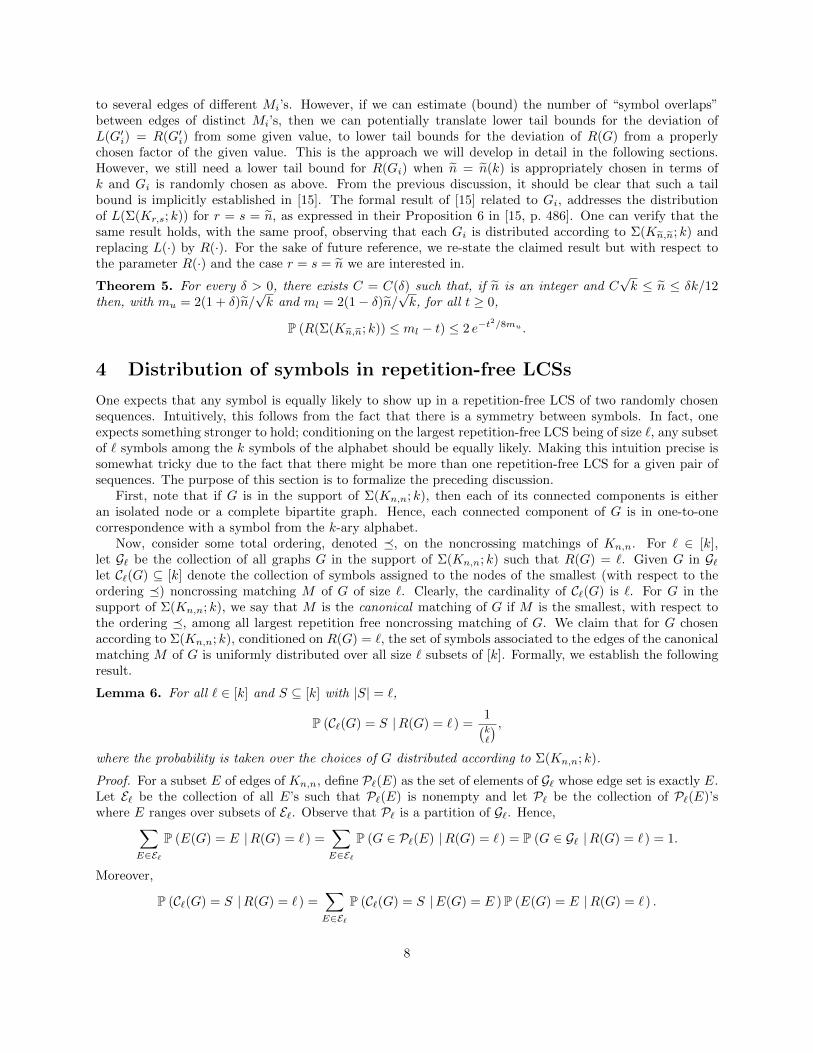
The random word model Σ(Kr,s; k),2 as introduced in [15], consists of the following (for an illustration,see Figure 1): the distribution over the set of subgraphs of Kr,s obtained by uniformly and independentlyassigning to each vertex of Kr,s one of k symbols and keeping those edges whose endpoints are associated tothe same symbol.

a

b a c

ba

a

Figure 1: Graph obtained from Σ(K4,3; 3) for the choice of symbols associated (shown close to) each node.

Following [15], two distinct edges ab and a′b′ of G are said to be noncrossing if a and a′ are in the sameorder as b and b′. In other words, if a < a′ and b < b′, or a′ < a and b′ < b. A matching of G is callednoncrossing if every distinct pair of its edges is noncrossing.

Henceforth, for a bipartite graph G, we denote by L(G) the number of edges in a maximum size (largest)noncrossing matching of G. To G chosen according to Σ(Kn,n; k) we can associate two sequences of length n,say x(G) and y(G), one for each of the bipartition sides of G, consisting of the symbols associated tothe vertices of Kn,n. Note that x(G) and y(G) are uniformly and independently distributed sequencesof n symbols over a k-ary alphabet. Observe that, if G is chosen according to Σ(Kn,n; k), then L(G) isprecisely the length of an LCS of its two associated sequences x(G) and y(G), and vice versa. Formally,L(G) = Ln(x(G), y(G)), where Ln(·, ·) is as defined in the introductory section.

Among other things, in [15], it is shown that L(Σ(Kn,n; k))√k/n is approximately equal to 2 when n

and k are very large, provided that n is “sufficiently large” compared to k. This result is formalized in thefollowing:

Theorem 4 (Kiwi, Loebl, and Matousek [15]). For every ε > 0, there exist k0 and C such that, for allk > k0 and all n with n > C

√k,

(1− ε) · 2n√k≤ E (L(Σ(Kn,n; k))) ≤ (1 + ε) · 2n√

k. (3)

Moreover, there is an exponentially small tail bound; namely, for every ε > 0, there exists c > 0 such thatfor k and n as above,

P(∣∣∣∣L(Σ(Kn,n; k))− 2n√

k

∣∣∣∣ ≥ ε 2n√k

)≤ e−cn/

√k.

Observe now that a graph G chosen according to Σ(Kn,n; k) has symbols, from a k-ary alphabet, implicitlyassociated to each of its nodes (to the jth node of each side of G the jth symbol of the correspondingsequence x(G) or y(G)). Furthermore, the endpoints of an edge e of G must, by construction, be associated

2Remember that Kr,s denotes the complete bipartite graph with two bipartition classes, one of size r and the other of size s.

6

to the same symbol, henceforth referred to the symbol associated to e. We say that a noncrossing matching ofG is repetition-free if the symbols associated to its edges are all distinct, and we denote by R(G) the numberof edges in a maximum size (largest) repetition-free noncrossing matching of G. If G is chosen accordingto Σ(Kn,n; k), then R(G) is precisely the length of a repetition-free LCS of its two associated sequencesx(G) and y(G), and vice versa. Formally, R(G) = Rn(x(G), y(G)), where again Rn(·, ·) is as defined in theintroductory section. Summarizing, we have reformulated the repetition-free LCS problem as an equivalentone, but concerning repetition-free noncrossing matchings. This justifies why, from now on, we will speakinterchangeably about repetition-free LCSs and repetition-free noncrossing matchings.

Clearly, for every G in the support of Σ(Kn,n; k) we always have that R(G) ≤ L(G). So, the upper boundin (3) for E (L(Σ(Kn,n; k))) and the upper tail bound for L(Σ(Kn,n; k)) of Theorem 4 are valid replacingL(Σ(Kn,n; k)) by R(Σ(Kn,n; k)). This explains why from now on we concentrate exclusively in the derivationof lower bounds such as those of Theorem 4 but concerning R(·).

Our approach partly builds on [15], so to help the reader follow the rest of this work, it will be convenientto have a high level understanding of the proofs of the lower bounds in Theorem 4. We next provide such ageneral overview. For precise statements and detailed proofs, see [15].

The proof of the lower bound in (3) has two parts, both of which consider a graph G chosen accordingto Σ(Kn,n; k) whose sides, say A and B, are partitioned into segments A1, A2, . . . and B1, B2, . . ., respectively,of roughly the same appropriately chosen size n = n(k). For each i, one considers the subgraph of G inducedby Ai ∪Bi, say Gi, and observes that the union of noncrossing matchings, one for each Gi, is a noncrossingmatching of G. The first part of the proof argument is a lower bound on the expected length of a largestnoncrossing matching of Gi. The other part of the proof is a lower bound on the expected length of alargest noncrossing matching of G which follows simply by summing the lower bounds from the first partand observing that, by “sub-additivity”,

∑i L(Gi) ≤ L(G).

Since the size of the segments A1, A2, . . . and B1, B2, . . . is n, there are n/n such segments in A and in B.An edge of Kn,n is in G with probability 1/k. So the expected number of edges in Gi is n2/k. The value of nis chosen so that, for each i, the expected number of edges of Gi is large, and the expected degree of eachvertex of Gi is much smaller than 1. Let G′i be the graph obtained from Gi by removing isolated vertices andthe edges incident to vertices of degree greater than 1. By the choice of n, almost all nonisolated verticesof Gi have degree 1. So G′i has “almost” the same expected number of edges as Gi, i.e. n2/k edges. Also,note that G′i is just a perfect matching (every node has degree exactly 1). This perfect matching, of sizesay t, defines a permutation of [t] — in fact, by symmetry arguments it is easy to see that, conditioning on t,the permutation is uniformly distributed among all permutations of [t]. Observe that a noncrossing matchingof G′i corresponds to an increasing sequence in the aforementioned permutation, and vice versa. So a largestnoncrossing matching of G′i is given by a Longest Increasing Sequence (LIS) of the permutation. There areprecise results (by Baik et al. [3]) on the distribution of the length of a LIS of a randomly chosen permutationof [t]. The expected length of a LIS for such a random permutation is 2

√t. So a largest noncrossing matching

in G′i has expected length almost 2√n2/k = 2n/

√k. As the number of i’s is n/n, we obtain a lower bound

of almost (n/n)2n/√k = 2n/

√k for the expected length of a largest noncrossing matching of G. The same

reasoning (although technically significantly more involved) yields a lower tail bound for the deviation of∑i L(G′i) ≤

∑i L(Gi) ≤ L(G) from 2n/

√k. This concludes our overview of the proof arguments of [15] for

deriving the lower bounds of Theorem 4.We now stress one important aspect of the preceding paragraph discussion. Namely, that by construction

G′i is a subgraph of Gi whose vertices all have degree one, and, moreover, G′i is in fact an induced subgraphof G. Since G is generated according to Σ(Kn,n; k), it must necessarily be the case that the symbols associatedto the edges of G′i are all distinct. Hence, a noncrossing matching of G′i is also a repetition-free noncrossingmatching of G′i, thence also of Gi. In other words, it holds that L(G′i) = R(G′i) ≤ R(Gi). Thus, a lowertail bound for the deviation of L(G′i) from 2n/

√k is also a lower tail bound for the deviation of R(Gi) from

2n/√k. Unfortunately, R(·) is not sub-additive as L(·) above (so now,

∑iR(Gi) is not necessarily a lower

bound for R(G)). Indeed, the union of repetition-free noncrossing matchings Mi of the Gi’s is certainly anoncrossing matching, but is not necessarily repetition-free. This happens because although the symbolsassociated to the edges of each Mi must be distinct, it might happen that the same symbol is associated

7

to several edges of different Mi’s. However, if we can estimate (bound) the number of “symbol overlaps”between edges of distinct Mi’s, then we can potentially translate lower tail bounds for the deviation ofL(G′i) = R(G′i) from some given value, to lower tail bounds for the deviation of R(G) from a properlychosen factor of the given value. This is the approach we will develop in detail in the following sections.However, we still need a lower tail bound for R(Gi) when n = n(k) is appropriately chosen in terms ofk and Gi is randomly chosen as above. From the previous discussion, it should be clear that such a tailbound is implicitly established in [15]. The formal result of [15] related to Gi, addresses the distributionof L(Σ(Kr,s; k)) for r = s = n, as expressed in their Proposition 6 in [15, p. 486]. One can verify that thesame result holds, with the same proof, observing that each Gi is distributed according to Σ(Kn,n; k) andreplacing L(·) by R(·). For the sake of future reference, we re-state the claimed result but with respect tothe parameter R(·) and the case r = s = n we are interested in.

Theorem 5. For every δ > 0, there exists C = C(δ) such that, if n is an integer and C√k ≤ n ≤ δk/12

then, with mu = 2(1 + δ)n/√k and ml = 2(1− δ)n/

√k, for all t ≥ 0,

P (R(Σ(Kn,n; k)) ≤ ml − t) ≤ 2 e−t2/8mu .

4 Distribution of symbols in repetition-free LCSs

One expects that any symbol is equally likely to show up in a repetition-free LCS of two randomly chosensequences. Intuitively, this follows from the fact that there is a symmetry between symbols. In fact, oneexpects something stronger to hold; conditioning on the largest repetition-free LCS being of size `, any subsetof ` symbols among the k symbols of the alphabet should be equally likely. Making this intuition precise issomewhat tricky due to the fact that there might be more than one repetition-free LCS for a given pair ofsequences. The purpose of this section is to formalize the preceding discussion.

First, note that if G is in the support of Σ(Kn,n; k), then each of its connected components is eitheran isolated node or a complete bipartite graph. Hence, each connected component of G is in one-to-onecorrespondence with a symbol from the k-ary alphabet.

Now, consider some total ordering, denoted , on the noncrossing matchings of Kn,n. For ` ∈ [k],let G` be the collection of all graphs G in the support of Σ(Kn,n; k) such that R(G) = `. Given G in G`let C`(G) ⊆ [k] denote the collection of symbols assigned to the nodes of the smallest (with respect to theordering ) noncrossing matching M of G of size `. Clearly, the cardinality of C`(G) is `. For G in thesupport of Σ(Kn,n; k), we say that M is the canonical matching of G if M is the smallest, with respect tothe ordering , among all largest repetition free noncrossing matching of G. We claim that for G chosenaccording to Σ(Kn,n; k), conditioned on R(G) = `, the set of symbols associated to the edges of the canonicalmatching M of G is uniformly distributed over all size ` subsets of [k]. Formally, we establish the followingresult.

Lemma 6. For all ` ∈ [k] and S ⊆ [k] with |S| = `,

P (C`(G) = S |R(G) = ` ) =1(k`

) ,where the probability is taken over the choices of G distributed according to Σ(Kn,n; k).

Proof. For a subset E of edges of Kn,n, define P`(E) as the set of elements of G` whose edge set is exactly E.Let E` be the collection of all E’s such that P`(E) is nonempty and let P` be the collection of P`(E)’swhere E ranges over subsets of E`. Observe that P` is a partition of G`. Hence,∑

E∈E`

P (E(G) = E |R(G) = ` ) =∑E∈E`

P (G ∈ P`(E) |R(G) = ` ) = P (G ∈ G` |R(G) = ` ) = 1.

Moreover,

P (C`(G) = S |R(G) = ` ) =∑E∈E`

P (C`(G) = S |E(G) = E )P (E(G) = E |R(G) = ` ) .

8

Thus, the desired conclusion will follow immediately once we show that P (C`(G) = S |E(G) = E ) = 1/(k`

)for all E ∈ E`. Indeed, let E ∈ E` and observe that the condition E(G) = E uniquely determines thecanonical noncrossing matching of G of size `, say M = M(G). Moreover, note that any choice of distinct `symbols to each of the ` distinct components of G to which the edges of M belong is equally likely. Sincethere are

(k`

)possible choices of `-symbol subsets of [k], the desired conclusion follows.

The preceding result will be useful in the next section in order to address the following issue. For Gand G1, . . . , Gb as defined in Section 3, suppose that M1, . . . ,Mb are the largest repetition-free noncrossingmatchings ofG1, . . . , Gb, respectively. As mentioned before the unionM of theMi’s is a noncrossing matchingof G, but not necessarily repetition-free. Obviously, we can remove edges from M , keeping one edge for eachsymbol associated to the edges of M , and thus obtain a repetition-free noncrossing matching M ′ containedin M , and thence also in G. Clearly, it is of interest to determine the expected number of edges that areremoved from M to obtain M ′, i.e. |M \M ′|, and in particular whether this number is small. Lemma 6 ismotivated, and will be useful, in this context. The reason being that, conditioning on the size si of the largestrepetition-free noncrossing matching in each Gi, it specifies the distribution of the set of symbols Csi(Gi)associated to the edges of the canonical noncrossing matching of Gi. The latter helps in the determinationof the sought-after expected value, since

|M \M ′| =b∑i=1

|Csi(Gi)| −∣∣∪bi=1Csi(Gi)

∣∣ .5 Tail bounds

In this section we derive bounds on the probability that R(G) is bounded away from its expected valuewhen G is chosen according to Σ(Kn,n; k). We will ignore the case where n = O(

√k) due to its limited

interest and the impossibility of deriving meaningful asymptotic results. Indeed, if n ≤ C√k for some positive

constant C and sufficiently large k, then the expected number of edges of a graph G chosen according toΣ(Kn,n; k) is n2/k ≤ C2 (just observe that there are n2 potential edges and that each one occurs in G with

probability 1/k). Since 0 ≤ R(G) ≤ |E(G)|, when n = O(√k), the expected length of a repetition-free

LCS will be constant — hence, not well suited for an asymptotic study. Thus, we henceforth assume thatn = ω(

√k). If in addition n = o(k), then Theorem 5 already provides the type of tail bounds we are looking

for. Hence, we need only consider the case where n = Ω(k). We will show that three different regimes arise.The first one corresponds to n = o(k

√k). For this case we show that the length of a repetition-free LCS

is concentrated around its expected value, which in fact is roughly 2n/√k (i.e. the same magnitude as that

of the length of a standard LCS). The second one corresponds to n = Θ(k√k). For this regime we show

that the length of a repetition-free LCS cannot be much smaller than a fraction of k, and we relate theconstant of proportionality with the constant hidden in the asymptotic dependency n = Θ(k

√k). The last

regime corresponds to n = (1 + Ω(1))k√k ln k. For this latter case we show that with high probability a

repetition-free LCS is of size k.

Throughout this section, n and k are positive integers, G is a bipartite graph chosen according toΣ(Kn,n; k), and G1, . . . , Gb are as defined in Section 3, where b is an integer approximately equal to n/n.Note in particular that Gi is distributed according to Σ(Kn,n; k).

This section’s first formal claim is motivated by an obvious fact; if r = R(G) is “relatively small”, thenat least one of the two following situations must happen:

• For some i ∈ [b], the value of ri = R(Gi) is “relatively small”.

• The sets of symbols, Cri(Gi), associated to the edges of the canonical largest noncrossing matching ofGi, for i ∈ [b], have a “relatively large” overlap, more precisely, the cardinality of Cr(G) is “relativelysmall” compared to the sum, for i ∈ [b], of the cardinalities of Cri(Gi).

9

The next result formalizes the preceding observation. In particular, it establishes that the probability thatR(G) is “relatively small” is bounded by the probability that one of the two aforementioned cases occurs(and also gives a precise interpretation to the terms “relatively large/small”).

Lemma 7. Let b be a positive integer. For a ≥ 0 and r ≥ t ≥ 0, let

P1 = P1(r, t)def=

∑r1,...,rb≥0

r1+···+rb=br−tc

P (R(Gi) ≤ ri,∀i ∈ [b]) , (Definition of P1)

P2 = P2(a, r, t)def= P

(R(G) ≤ r − a,

b∑i=1

R(Gi) ≥ r − t

). (Definition of P2)

Then,

P (R(G) ≤ r − a) ≤ P1 + P2.

Proof. Just note that

P (R(G) ≤ r − a) = P

(R(G) ≤ r − a,

b∑i=1

R(Gi) < dr − te

)+ P

(R(G) ≤ r − a,

b∑i=1

R(Gi) ≥ dr − te

)

≤ P

(b∑i=1

R(Gi) < r − t

)+ P

(R(G) ≤ r − a,

b∑i=1

R(Gi) ≥ r − t

).

The desired conclusion follows observing that the two last terms in the preceding displayed expression areequal to P1 and P2, respectively.

The following lemma will be useful in bounding the terms in P1, i.e. the probability that R(Gi) is“relatively small” for some i. Henceforth, for the sake of clarity of exposition, we will ignore the issue ofintegrality of quantities (since we are interested in the case where n is large, ignoring integrality issues shouldhave a negligible and vanishing impact in the following calculations).

Lemma 8. Let δ > 0 and n = n(k) be such that it satisfies the hypothesis of Theorem 5 and let ml =

(1− δ)2n/√k. Let b = b(k)

def= n/n. Then,

P1 = P1(bml, t) ≤ (2e(ml + 1))b

exp

(− t2

16(1 + δ)n/√k

).

Proof. Observe that, by independence of the R(Gi)’s and Theorem 5, for mu = (1 + δ)2n/√k,

P (R(Gi) ≤ ri,∀i ∈ [b]) = P (R(Gi) ≤ ml − (ml − ri),∀i ∈ [b])

≤b∏i=1

(2e−max0,ml−ri2/8mu

)= 2be−

∑bi=1 max0,ml−ri2/8mu .

By Cauchy-Schwarz, since max0, x+ max0, y ≥ max0, x+ y, and assuming that∑bi=1 ri = bbml − tc,

b∑i=1

max0,ml − ri2 ≥1

b

(b∑i=1

max0,ml − ri

)2

≥ 1

bt2.

Recalling that there are(M+b−1b−1

)≤(M+bb

)ways in which b nonnegative summands can add up to M ∈ N,

and that(µν

)≤ (eµ/ν)ν ,

P1 ≤∑

r1,...,rb≥0

r1+···+rb=bbml−tc

2be−t2/8bmu ≤

(bbml − tc+ b

b

)2be−t

2/8bmu ≤ (2e(ml + 1))be−t

2/8bmu .

Since mu = (1 + δ)2n/√k and bn = n, the desired conclusion follows immediately.

10

The next lemma will be useful in bounding P2, i.e. the probability that the sets of symbols associated tothe edges of the canonical largest noncrossing Gi’s matchings have a “relatively large” overlap. The resultin fact shows how to translate tail bounds for an urn occupancy model into bounds for P2.

Lemma 9. If b is a positive integer, a ≥ 0, r ≥ t ≥ 0, and s = dr − te, then

P2 = P2(a, r, t) ≤ P(k − Y (k,s) ≤ r − a

).

Proof. Clearly,

P2 =∑

s1,...,sb≥0

s1+···+sb≥r−t

P (R(G) ≤ r − a |R(Gi) = si,∀i ∈ [b] )P (R(Gi) = si,∀i ∈ [b]) .

Let C`(·) be as defined in Section 4. Note that if we take the union of noncrossing matchings, one Mi foreach Gi, we get a noncrossing matching M = ∪iMi of G. However, the edges of M do not necessarily havedistinct associated symbols. By throwing away all but one of the edges of M associated to a given symbol,one obtains a repetition-free noncrossing matching of G. It follows that, conditioning on R(Gi) = si for alli ∈ [b],

R(G) ≥

∣∣∣∣∣b⋃i=1

Csi(Gi)

∣∣∣∣∣ .Thus,

P (R(G) ≤ r − a |R(Gi) = si,∀i ∈ [b] ) ≤ P

(∣∣∣∣∣b⋃i=1

Csi(Gi)

∣∣∣∣∣ ≤ r − a |R(Gi) = si,∀i ∈ [b]

)

= P

(∣∣∣∣∣b⋃i=1

Csi(Gi)

∣∣∣∣∣ ≤ r − a | |Csi(Gi)| = si,∀i ∈ [b]

).

Let ~s = (s1, . . . , sb). We claim that∣∣∣⋃bi=1 Csi(Gi)

∣∣∣ conditioned on |Csi(Gi)| = si, for all i ∈ [b], is distributed

exactly as the number of nonempty urns left when the Grouped Urn (k,~s)-model (as defined in Section 4)ends, i.e. is distributed as the random variable k −X(k,~s) (where X(k,~s) is as defined in Section 4). Indeed,it suffices to note that by Proposition 3, conditioned on |Csi(Gi)| = si, the set Si = Csi(Gi) is a randomly

and uniformly chosen subset of [k] of size si, and that k −X(k,~s) is distributed exactly as∣∣∣⋃bi=1 Csi(Gi)

∣∣∣. It

follows, from the forgoing discussion and Lemma 2, that

P (R(G) ≤ r − a |R(Gi) = si, i ∈ [b] ) = P(k −X(k,~s) ≤ r − a

)≤ P

(k − Y (k,s) ≤ r − a

).

The next result establishes the first of the announced tail bounds, for the first of the three regimesindicated at the start of this section. An interesting aspect, that is not evident from the theorem’s statement,is the following fact that is implicit in its proof; if the speed of growth of n as a function of k is not toofast, then we may choose b as a function of k so that

∑bi=1R(Gi) is roughly (with high probability) equal

to R(G). In particular, the proof argument rests on the fact that, for an appropriate choice of parameters, thecanonical largest noncrossing matching of Gi is of size approximately 2(n/b)/

√k, and with high probability

there is very little overlap between the symbols associated to the edges of the canonical largest noncrossingmatchings of distinct Gi’s.

Theorem 10. If n = o(k√k), then for every 0 < ξ ≤ 1 there is a sufficiently large constant k0 = k0(ξ) such

that, for all k > k0,

P(R(G) ≤ (1− ξ)2n/

√k)≤ 2e−

110 ξ

22n/√k.

11

Proof. Let c > 1 be large enough so (1 − 1/c)2 ≥ (9/10)(1 + ξ/c). Let δ = ξ/c and t = (1 − 1/c)ξ2n/√k.

Now, choose n = n(k) = k3/4 (instead of 3/4, any exponent strictly between 1/2 and 1 suffices). Note that

one can choose k0 (depending on ξ through δ) so that for all k ≥ k0 the conditions on n of Theorem 5 aresatisfied. Let ml and mu be as in Theorem 5. Note that ml = (1−ξ/c)2n/

√k = Θ(k1/4), b = n/n = n/k3/4,

and bmu = (1 + ξ/c)2n/√k. Hence, by Lemma 8,

P1 ≤ exp

(b ln(2e(ml + 1)))− t2

8bmu

)= exp

(n√k

Θ(k−1/4 ln k

)− (1− 1/c)2ξ22n/

√k

8(1 + ξ/c)

).

Since k−1/4 ln k = o(1) and (1 − 1/c)2 ≥ (9/10)(1 + ξ/c), it follows that for a sufficiently large k′0 ≥ k0 itholds that for all k ≥ k′0,

P1 ≤ exp

(− (1− 1/c)2ξ22n/

√k

9(1 + ξ/c)

)≤ exp

(− 1

10ξ22n/

√k

).

On the other hand, since t = (1−1/c)ξ2n/√k, if we fix a = ξ2n/

√k, then we have that t−a ≤ −(ξ/c)2n/

√k.

Taking s = bml − t = (1− ξ)2n/√k ≤ 2n/

√k, as ξ ≤ 1, by Lemma 9 and Proposition 3, Part 3,

P2 ≤ P(k − Y (k,s) ≤ bml − a

)= P

(k − Y (k,s) ≤ s+ t− a

)≤ P

(k − Y (k,s) ≤ s− ξ2n

c√k

)≤(

2cen

ξk√k

)(ξ/c)2n/√k

.

Let k′′0 be sufficiently large (depending on ξ) so that 2cen/(ξk√k) ≤ e−cξ/10 for all k ≥ k′′0 (such a k′′0 exists

because n = o(k√k)). It follows that for k ≥ k′′0 we can upper bound P2 by exp

(− 1

10ξ22n/

√k)

.

Since by Lemma 7 we know that P(R(G) ≤ (1− ξ)2n/

√k)≤ P1 + P2, it follows that for k ≥ k0 =

k0(ξ)def= maxk′0, k′′0 we get the claimed bound.

Next, we consider a second regime, but first we establish an inequality that we will soon apply.

Claim 11. For every 0 ≤ x ≤ 1 and ρ ≥ 0,

e−ρ(1−x) − e−ρ − x(1− e−ρ) ≤ 0.

Proof. Since 0 ≤ x ≤ 1, it holds that 0 ≤ xn ≤ x for all n ∈ N \ 0. Then, since ey =∑n∈N y

n/n! andperforming some basic arithmetic,

eρx − 1− x(eρ − 1) =∑n≥1

ρn

n!(xn − x) ≤ 0.

Multiplying by e−ρ, the claimed result immediately follows.

Theorem 12. Let ρ > 0 and 0 < ξ < 1. If n = 12ρk√k, then there is a sufficiently large constant

k0 = k0(ρ, ξ) such that for all k > k0,

P(R(G) ≤ (1− ξ)k(1− e−ρ)

)≤ 2e−

ξ2

32(1+ξ/12)k(1−e−ρ) ≤ 2e−

135 ξ

2k(1−e−ρ).

Proof. Since ξ < 1, the second stated inequality follows immediately from the first one. We thus focus onestablishing the first stated inequality.

Let δ = ξ/12. Now, choose n = k3/4 (instead of 3/4, any exponent strictly between 1/2 and 1 suffices)and set b = n/n. Note that one can choose k′0 (depending on ξ through δ) so that for all k > k′0 the conditions

12

on n = n(k) of Theorem 5 are satisfied. Let ml = (1 − δ)2n/√k and observe that bml = (1 − δ)2n/

√k =

(1−ξ/12)ρk. Choose t = (2ξ/3)ρk and note that s = bml−t = (1−3ξ/4)ρk. Let λ = E(Y (k,s)

)= k(1−1/k)s

be as in Proposition 3. We claim that for 0 < ξ < 1,

λ ≤ ke−ρ + (3ξ/4)k(1− e−ρ). (4)

Indeed, since 1 + x ≤ ex we have that λ = k(1 − 1/k)s ≤ ke−ρ(1−3ξ/4), so to prove (4) it suffices to recallthat by Claim 11 we have that e−ρ(1−3ξ/4) ≤ e−ρ + (3ξ/4)(1− e−ρ).

Now, fix a and a so a = ξk(1− e−ρ) and a = bml − k(1− e−ρ) + a. By Lemma 9 and (4),

P2 ≤ P(k − Y (k,s) ≤ bml − a

)= P

(Y (k,s) ≥ ke−ρ + a

)≤ P

(Y (k,s) ≥ λ+ (ξ/4)k(1− e−ρ)

).

Hence, taking p = λ/k ≤ 1, q = 1− p, and applying Proposition 3, Part 1,

P2 ≤ exp

(− ξ2(1− e−ρ)2k

32(pq + (ξ/12)(1− e−ρ))

)≤ exp

(− ξ2(1− e−ρ)2k

32(q + (ξ/12)(1− e−ρ))

).

Again by Proposition 3, we know that λ = k(1 − 1/k)s. Thus, recalling that by our choice of parameterss = (1−3ξ/4)ρk and since (1−1/k)s = (1−1/k)ρ(1−3ξ/4)k converges to e−ρ(1−3ξ/4) > e−ρ when k goes to∞,it follows that q = 1−p = 1−(1−1/k)s can be upper bounded by 1−e−ρ for all k > k′′0 and some sufficientlylarge k′′0 > k′0 (depending on ξ). Hence, for k > k′′0 it holds that q + (ξ/12)(1− e−ρ) ≤ (1 + ξ/12)(1− e−ρ),and

P2 ≤ exp

(− ξ2

32(1 + ξ/12)k(1− e−ρ)

).

We will now upper bound P1. Note that, by our choice for n and the hypothesis on n, we have ml =(1 − ξ/12)2n/

√k = (1 − ξ/12)k1/4 ≤ k, b = n/n ≤ ρk3/4, and bmu = (1 + ξ/12)2n/

√k = (1 + ξ/12)ρk.

Recalling that we fixed t = (2ξ/3)ρk, by Lemma 8,

P1 ≤ exp

(b ln(2e(ml + 1)))− t2

8bmu

)≤ exp

(ρk3/4 ln(2e(k + 1)))− ξ2ρk

18(1 + ξ/12)

).

Since k3/4 ln(2e(k + 1)) = o(k) and because 1 − e−ρ ≤ ρ, it follows that for a sufficiently large k′′′0 it holdsthat for all k > k′′′0 ,

P1 ≤ exp

(− ξ2

19(1 + ξ/12)ρk

)≤ exp

(− ξ2

19(1 + ξ/12)k(1− e−ρ)

).

Since P (R(G) ≤ (1− ξ)k(1− e−ρ)) ≤ P1 + P2 for k > k0 = k0(ρ, ξ)def= maxk′′0 , k′′′0 , we get the claimed

bound.

Our next result establishes that if n is sufficiently large with respect to k, then with high probability therepetition-free LCS is of size k, i.e. it is a permutation of the underlying alphabet. Moreover, the theorem’sproof implicitly shows something stronger; if the speed of growth of n as a function of k is fast enough, thenwe may choose b as a function of k so that with high probability every symbol of the k-ary alphabet showup in association to an edge of a canonical maximum size matching of some Gi — chosen such edges oneobtains a noncrossing repetition free matching of G of the maximum possible size k.

Theorem 13. If n = (12 + ξ)k

√k ln k for some ξ > 0, then there is a sufficiently large constant k0 = k0(ξ)

such that for all k > k0,

P (R(G) 6= k) ≤ 2

kξ.

13

Proof. Let δ = δ(ξ) > 0 be such that (1 − δ)(1 + 2ξ) = 1 + 3ξ/2. Now, let n = k3/4 (instead of 3/4, anyexponent strictly between 1/2 and 1 suffices) and set b = n/n. Note that one can choose k′0 (depending on ξthrough δ) so that for all k > k′0 the conditions on n = n(k) of Theorem 5 are satisfied. Let ml = (1−δ)2n/

√k

be as in Theorem 5. Observe that bml = (1 − δ)2n/√k = (1 + 3ξ/2)k ln k. Choose t = (ξ/2)k ln k so that

s = bml − t = (1 + ξ)k ln k. Fix a so k − bml + a = 1. By Lemma 9 and Proposition 3, Part 2,

P2 ≤ P(Y (k,s) ≥ k − bml + a

)= P

(Y (k,s) 6= 0

)≤ 1

kξ.

By the hypothesis on n and the choice of n, we have that b = n/n = (12 + ξ)k3/4 ln k, so recalling that

ml = (1− δ)2n/√k = (1− δ)2k1/4,

b ln(2e(ml + 1)) = O(k3/4 ln2 k) = o(k ln k).

Furthermore, let mu = (1 + δ)2n/√k be as in Theorem 5. Thus,

t2

16(1 + δ)n/√k

=t2

8bmu=

ξ2k ln k

32(1 + δ)(1 + 2ξ).

Hence, by Lemma 8, for a sufficiently large constant k′′0 (again depending on ξ through δ), we can guaranteethat, for all k > k′′0 ,

P1 ≤ (2e(ml + 1))be−t2/8bmu = exp

(b ln(2e(ml + 1))− t2

8bmu

)≤ 1

kξ.

Summarizing, for k > k0 = k0(ξ)def= maxk′0, k′′0, we get that P (R(G) 6= k) ≤ P1 + P2 ≤ 2/kξ.

From the lower tail bounds for R(G) obtained above, one can easily derive lower bounds on the expectedvalue of R(G) via the following well-known trick.

Lemma 14. If X is a nonnegative random variable and x > 0, then E (X) ≥ x (1− P (X ≤ x)).

Proof. Let IA denote the indicator of the event A occurring. Just observe that

E (X) = E(XIX≤x

)+ E

(XIX>x

)≥ xE

(IX>x

)= x (1− P (X ≤ x)) .

Theorem 1 now follows as a direct consequence of the preceding lemma, Theorems 10, 12, and 13, andthe fact that R(G) ≤ k.

Acknowledgements

The authors would like to thank Carlos E. Ferreira, Yoshiharu Kohayakawa, and Christian Tjandraatmadjafor some discussions in the preliminary stages of this work.

References

[1] S. Adi, M. Braga, C. Fernandes, C. Ferreira, F. Martinez, M.-F. Sagot, M. Stefanes, C. Tjandraatmadja,and Y. Wakabayashi. Repetition-free longest common subsequence. Discrete Appl. Math., 158(12):1315–1324, 2010.

[2] S. Angibaud, G. Fertin, I. Rusu, A. Thvenin, and S. Vialette. On the approximability of comparinggenomes with duplicates. J. Graph Algorithms Appl., 13(1):19–53, 2009.

14

[3] J. Baik, P. Deift, and K. Johansson. On the distribution of the length of the longest increasing subse-quence of random permutations. J. Amer. Math. Soc., 12:1119–1178, 1999.

[4] L. Bergroth, H. Hakonen, and T. Raita. A survey of longest common subsequence algorithms. InProceedings of the 7th International Symposium on String Processing Information Retrieval (SPIRE),pages 39–48, 2000.

[5] G. Blin, P. Bonizzoni, R. Dondi, and F. Sikora. On the parameterized complexity of the repetition freelongest common subsequence problem. Information Processing Letters, 112(7):272–276, 2012.

[6] P. Bonizzoni, G. Della Vedova, R. Dondi, G. Fertin, R. Rizzi, and S. Vialette. Exemplar longest commonsubsequence. IEEE/ACM Trans. Comput. Biol. Bioinformatics, 4(4):535–543, 2007.

[7] P. Bonizzoni, G. Della Vedova, R. Dondi, and Y. Pirola. Variants of constrained longest commonsubsequence. Information Processing Letters, 110(20):877–881, 2010.

[8] R. Boppana. Eigenvalues and graph bisection: An average-case analysis. In Proceedings of the 28thAnnual Symposium on Foundations of Computer Science (FOCS), pages 280–285. IEEE ComputerSociety, 1987.

[9] T. Bui, S. Chaudhuri, T. Leighton, and M. Sipser. Graph bisection algorithms with good average casebehavior. Combinatorica, 7(2):171–191, 1987.

[10] A. Coja-Oghlan. A spectral heuristic for bisecting random graphs. Random Struct. Algorithms,29(3):351–398, 2006.

[11] A. Condon and R. Karp. Algorithms for graph partitioning on the planted partition model. RandomStruct. Algorithms, 18(2):116–140, 2001.

[12] W. Feller. An introduction to Probability Theory and its Applications, volume 1. John Wiley & Sons,third edition, 1968.

[13] S. Janson. Large deviation inequalities for sums of indicator variables. Technical Report 1994:34,Uppsala U., 1994. Available at http://www2.math.uu.se/∼svante/papers/sj107.ps.

[14] M. Jerrum and G. B. Sorkin. Simulated annealing for graph bisection. In Proceedings of the 34th AnnualSymposium on Foundations of Computer Science (FOCS), pages 94–103. IEEE Computer Society, 1993.

[15] M. Kiwi, M. Loebl, and J. Matousek. Expected length of the longest common subsequence for largealphabets. Adv. Math., 197:480–498, 2005.

[16] D. Sankoff. Genome rearrangement with gene families. Bioinformatics, 15(11):909–917, 1999.

[17] D. Sankoff. Gene and genome duplication. Current Opinion in Genetics & Development, 11(6):681–684,2001.

[18] D. Sankoff and J. Kruskal, editors. Common subsequences and monotone subsequences, chapter 17,pages 363–365. Addison–Wesley, Reading, Mass., 1983.

15