arX

iv:n

lin/0

0120

46v1

[nl

in.S

I] 2

2 D

ec 2

000

Algebraic approach in the study of time-dependent nonlinearintegrable systems: Case of the singular oscillator

Jayendra N. Bandyopadhyay∗, A. Lakshminarayan and Vijay B. SheoreyPhysical Research Laboratory,

Navrangpura, Ahmedabad 380 009, India.

(February 8, 2008)

Abstract

The classical and the quantal problem of a particle interacting in one-

dimension with an external time-dependent quadratic potential and a con-

stant inverse square potential is studied from the Lie-algebraic point of view.

The integrability of this system is established by evaluating the exact invariant

closely related to the Lewis and Riesenfeld invariant for the time-dependent

harmonic oscillator. We study extensively the special and interesting case of

a kicked quadratic potential from which we derive a new integrable, nonlin-

ear, area preserving, two-dimensional map which may, for instance, be used

in numerical algorithms that integrate the Calogero-Sutherland-Moser Hamil-

tonian. The dynamics, both classical and quantal, is studied via the time-

evolution operator which we evaluate using a recent method of integrating the

quantum Liouville-Bloch equations [1]. The results show the exact one-to-one

correspondence between the classical and the quantal dynamics. Our analysis

also sheds light on the connection between properties of the SU(1, 1) algebra

and that of simple dynamical systems.

PACS numbers : 03.65.-w, 03.65.Fd, 05.45.-a

Typeset using REVTEX

∗jayendra@prl.ernet.in

1

I. INTRODUCTION

The classical and quantum mechanical study of time-dependent Hamiltonian systemsare generic and important. They span a wide spectrum of subjects ranging from interactionbetween atoms and radiation [2,3], adiabatic [4,5] and non-adiabatic [6,7] Berry phase, time-dependent harmonic oscillators [8–10] and quantum motion of a particle in a Paul trap[11,12], to time-dependent mean-field theory (cranking model [13]) in particular and thetime-dependent shell model [14] in general.

The question of the existence of invariants (constants of motion) is one of central impor-tance in the study of any dynamical system, be it classical or quantal. A basic theorem ofclassical mechanics asserts that if the number of independent invariants, satisfying certainconditions, is equal to the number of degrees of freedom, then the motion can be reducedto quadratures, or equivalently, an action-angle transformation to a Hamiltonian dependentonly on the actions can be found [15]. Such systems are integrable.

The lack of sufficient number of invariants invariably leads to a phase space that has anonzero measure of chaotic trajectories [16]. For time-independent Hamiltonian systems theHamiltonian itself is an invariant. However, when the Hamiltonian is an explicit function oftime, it is no more an invariant, and this is of course a reflection of the non-conservation ofenergy. Various methods have been used to obtain approximate solutions for time-dependentproblems, e.g., the adiabatic approximation, the sudden approximation, time-dependentperturbation techniques, etc.

The most widely studied time-dependent Hamiltonian system is the time-dependentharmonic oscillator (TDHO). It has long been a problem of considerable interest becauseof its varied applications in different areas of physics, for instance in molecular physics,quantum chemistry, quantum optics and plasma physics. The Hamiltonian of this system isgiven by,

H(t) =1

2p2 +

1

2ω2(t) q2, (1)

where p and q are conjugate canonical variables. The adiabatic invariant for this system wasoriginally given at the first Solvay Congress in 1911 when the Hamiltonian of this systemwas used as an approximate Hamiltonian for the slowly lengthening pendulum [17].

The study of this one-dimensional TDHO was greatly advanced due to the work of Lewis[8,9] and Riesenfeld [10]. Lewis [8] determined the exact invariant by applying Kruskal’sasymptotic method [18] and showed that a previously known adiabatic invariant was in factan exact invariant. Later Lewis and Riesenfeld (LR) [10] determined that same invariant bystarting with the assumption of the existence of an explicitly time-dependent, homogeneousand quadratic invariant of the form given by,

I(t) =1

2[α(t) p2 + β(t) q2 + 2 γ(t) p q], (2)

where the coefficients α(t), β(t) and γ(t) are time-dependent real functions and I(t) satisfiesthe condition,

dI

dt≡ ∂I

∂t+ I,H(t) = 0. (3)

2

Here ∗, ∗ denotes the usual Poisson bracket. From the above two equations and after somecalculations they derived the exact invariant as,

I(t) =1

2

[

ρ2 p2 +

(

ρ2 +1

ρ2

)

q2 − 2 ρ ρ p q

]

, (4)

with ρ(t) satisfying the subsidiary condition

ρ + ω2(t) ρ − 1

ρ3= 0. (5)

This more complicated, nonlinear, differential equation represented an advance due to thereason that any particular solution ρ(t) of the above equation would give the exact invariantI(t) for all initial conditions of p and q.

The above technique actually predates the work of Lewis and Riesenfeld in a slightlydifferent context, and we briefly point this out. We note that the equation of motion ofthe TDHO is, d2q/dt2 + ω2(t) q = 0. This is of the same form as the time-independent,one-dimensional Schrodinger equation, if we assume that t represents the spatial coordinateand q, the wave-function. According to an early work by Milne (1930) [19], it is possible tosolve this Schrodinger equation using the knowledge of any particular solution of the Eq. (5),after proper identifications. Therefore, any particular solution of the subsidiary conditioncan also give the exact solution for the TDHO.

Lewis [9] attempted to give an interpretation of I(t) as the most general homogeneousquadratic invariant possible for the Hamiltonian of the one-dimensional TDHO. A morenatural and physical interpretation has been suggested by Eliezer and Gray [20] in termsof two-dimensional auxiliary motion, i.e., in terms of a two-dimensional uncoupled TDHO.They showed that the above subsidiary condition Eq. (5) is the radial equation of motion forthis two-dimensional system and the invariant I(t) is proportional to the conserved angularmomentum of this auxiliary motion. Gunther and Leach [21] interpreted I(t) in terms ofcanonical transformations and under their transformation the invariant I(t) became theHamiltonian of the one-dimensional time-independent harmonic oscillator of unit frequency.

Besides these previous interpretations of I(t), we can interpret the form of I(t) chosenby Lewis and Riesenfeld (LR) [10] from the Lie-algebraic point of view. The Hamiltonian ofthe one-dimensional TDHO is formed by the dynamical variables 1

2p2 and 1

2q2. These two

dynamical variables together with p q are generators of the closed SU(1, 1) algebra underthe Poisson bracket operation and I(t) was chosen in [10] as the linear combination of thesegenerators. Generalizing the LR-invariant from the Lie-algebraic point of view, we expectthat if any time-dependent Hamiltonian be the combination of the generators of any closedalgebra, an invariant would be a linear combination of the generators of that closed algebrawith time-dependent coefficients.

The integrability of the one-dimensional TDHO is not surprising, because this is a lin-ear system. We know, one-dimensional time-dependent Hamiltonians usually lead to non-integrability, e.g., a simple pendulum whose length varies in time. Except for the adiabaticor small oscillation approximations, this was the problem posed by Lorentz at the abovementioned Solvay congress and the solutions have the possibility of displaying chaos.

Now a natural question is if there exist one-dimensional time-dependent nonlinear Hamil-tonians which are also integrable? In fact, the singular oscillator with a centrifugal force

3

potential provides an important example whose kinematics is still within the SU(1, 1) alge-bra. In the second section, we have discussed such a nonlinear Hamiltonian and we have alsoderived its invariant from our new Lie-algebraic interpretation of the LR-invariant. Usingthis Hamiltonian we have constructed an integrable, area preserving, nonlinear map andderived its exact invariant with a knowledge of its fixed points.

We have determined the classical time-evolution (Perron-Frobenius) operator following arecent method elucidated by Rau [1]. This method was originally used for solving the quan-tum Liouville-Bloch equation, but we have applied this in the classical case and have beenable to show the one-to-one correspondence between this nonlinear map and the linear map(derived from the Hamiltonian of the one-dimensional TDHO). In the third section, we havestudied the quantum dynamics of the nonlinear map and again we have used Rau’s methodto determine the quantum time-evolution operator. This identical approach to classical andquantum dynamics helps us to show, rather trivially, the exact one-to-one correspondencebetween the classical and the quantal. Our study also has the dimension of interpreting themathematics of the SU(1, 1) algebra from a dynamical systems viewpoint. For instance,we derive powers of non-commuting products of exponentials of the SU(1, 1) algebra. Thisreveals when the powers can degenerate to the identity, something that is immediately clearfrom the dynamics of the underlying system due to the presence of degenerate periodicorbits.

II. THE CLASSICAL KICKED SINGULAR OSCILLATOR

First, we will describe the general Hamiltonian of which an important special case con-stitutes the rest of the paper. For the existence of an invariant for the one-dimensionalTDHO, the subsidiary condition Eq. (5) has to be integrated with some initial conditions,that is we should be able to determine a particular solution. The subsidiary condition, givenin Eq. (5), is a nonlinear, time-dependent, equation and its integrability is not immediatelyobvious. If we assume ρ as a position variable, say q, then Eq. (5) is the equation of motioncorresponding to the Hamiltonian given by,

H(t) =1

2

(

p2 +k

q2

)

+1

2ω2(t) q2, (6)

with k = 1. This is a time-dependent Hamiltonian, and has also been studied for long:it was studied in part by Lewis and Leach [22], Camiz et. al. and Pedrosa et. al. [23]studied this Hamiltonian quantum mechanically. The new nonlinear force in the system isa ‘Centrifugal force’ and it appears in many integrable systems, including the celebratedCalogero-Sutherland-Moser [24–26] many-body Hamiltonian.

The Hamiltonian in Eq. (6), is formed by the dynamical variables 1

2

(

p2 + kq2

)

and 1

2q2.

These two variables together with p q, also form the SU(1, 1) closed algebra. Following ouralgebraic interpretation of I(t), we can assume the invariant of this nonlinear Hamiltonianto be of the form,

I(t) =1

2α(t)

(

p2 +k

q2

)

+1

2β(t) q2 + 2 γ(t) p q. (7)

4

Again, by the same substitutions and identical procedures we get

I(t) =1

2ρ2

(

p2 +k

q2

)

+1

2

(

ρ2 +1

ρ2

)

q2 − ρ ρ p q, (8)

with the same subsidiary condition as given in Eq. (5). It is also possible to determine this in-variant using time-dependent canonical transformations [27], however, our algebraic methodaccomplishes this more elegantly. In this case, the equation of motion and the subsidiarycondition are the same nonlinear equation, but the fact that we need only one particularsolution of this equation to determine the invariant shows the power of the methodologyand the integrability of the above Hamiltonian in Eq. (6). In Fig. 1 we show a special casecorresponding to ω2(t) = 1 + cos(

√2 t) where the existence of the invariant is reflected in

the regular structures.

A. The integrable discrete system

Now we use the above to construct a nonlinear integrable map. Integrable discretesystems, or maps, have been intensely studied for some time now and many interestingmethods and results have been found. Integrable maps are important for the followingreasons. Firstly, studying the dynamics of a mapping is more simpler than the dynamicsof a continuous system since it involves direct iteration. Secondly, if one wants to studynumerically any integrable continuous system, it is absurd to use non-integrable numericalschemes which destroy the basic properties of the system. Therefore, for numerical studiesof any integrable system, one has to find a discrete integrable version of the system. Thediscrete map we discuss below, or extensions thereof, for instance, may be used in thenumerical studies of the Calogero-Sutherland-Moser model. Lastly, we can argue that thediscrete systems are more fundamental ones since they contain continuous ones as speciallimits.

Studying the stroboscopic map of any time-periodic system is always possible, at leastnumerically. To get an analytical expression a much studied form of the time dependenceis: ω2(t) = ω2 T

∑

n δ(t − nT ). The standard map and its quantization as well as anexperimental realization of the time-dependence through a periodically pulsed laser field[28] provides a well known example of this kind. The map corresponding to the TDHO is alinear map, which is very simple classically.

Here we will study the map corresponding to the nonlinear system. The Hamiltonian ofinterest is,

H(t) =1

2

(

p2 +k

q2

)

+1

2ω2 T q2

∑

n

δ(t − nT ), (9)

and the corresponding Hamilton’s equations of motion are,

p =k

q3− ω2 T q

∑

n

δ(t − nT ),

q = p. (10)

5

The equation of motion of the system is given by,

q + ω2 T q∑

n

δ(t − nT ) − k

q3= 0. (11)

This equation is the same as that of the subsidiary condition given in Eq. (5), except forthe constant k. Integrating Hamilton’s equations of motion from just after the n-th kick tojust after the (n + 1)-th kick and defining new scaled variables

p → k1

4 T−1

2 p, and q → k1

4 T1

2 q,

the phase space map of the system is,

qn+1 =

√

p2n +

1

q2n

+ q2n + 2pnqn,

pn+1 =p2

n + 1

q2n

+ pnqn

qn+1

− Ω2qn+1, (12)

where Ω = ω T .Note that the scaling has removed the k dependence, but that the scaling is singular at

k = 0 and in fact this limit leads to the removal of the 1/q2 term, as is discussed furtherbelow. If we plot this phase space map numerically, it clearly shows its regular behaviour,as illustrated in Fig. 2. This rather complicated looking discrete map has a very simplebehaviour, reflecting the fact that both this and a linear map, derivable from a TDHO, havecommon algebraic antecedents. This linear map is derived from the Hamiltonian in Eq. (9)by simply discarding the 1/q2 term (the k = 0 limit) and is given by

qn+1 = pn + qn,

pn+1 = pn − Ω2 qn+1. (13)

In fact the property of the linear map that exclusively quasi-periodic or entirely periodicbehaviour exists for different values of the parameter is also observed for the nonlinear map.For 0 < Ω2 < 4 the motion is bounded and stable and for all other values the motion isunbounded and unstable, in both the maps. The invariant in the case of the linear mapdescribes either an ellipse or a hyperbola, now we determine the invariant of the nonlinearmap using the method of LR.

Using Eq. (8) the invariant of this map would be of the form,

I = ρ2

(

pn2 +

1

qn2

)

+

(

ρ2 +1

ρ2

)

qn2 − 2 ρ ρ pn qn, (14)

where ρ satisfies the same subsidiary condition as given in Eq. (5), but now ω2(t) =ω2 T

∑

n δ(t − nT ). If we are able to determine any particular solution of the subsidiarycondition, then we can use that solution to get the invariant of the map Eq. (12). As wehave already mentioned, the equation of motion of this nonlinear kicked system is the sameas that of the subsidiary condition for ρ, as shown in Eq. (11), therefore if we are able toget any solution of the nonlinear map Eq. (12), that solution should also be the solution

6

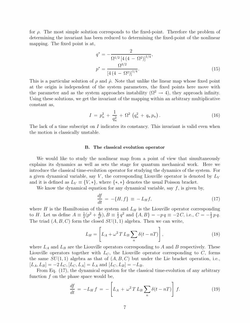
for ρ. The most simple solution corresponds to the fixed-point. Therefore the problem ofdetermining the invariant has been reduced to determining the fixed-point of the nonlinearmapping. The fixed point is at,

q∗ = − 2

Ω1/2 [4 (4 − Ω2)]1/4,

p∗ =Ω3/2

[4 (4 − Ω2)]1/4. (15)

This is a particular solution of ρ and ρ. Note that unlike the linear map whose fixed pointat the origin is independent of the system parameters, the fixed points here move withthe parameter and as the system approaches instability (Ω2 → 4), they approach infinity.Using these solutions, we get the invariant of the mapping within an arbitrary multiplicativeconstant as,

I = p2

n +1

q2n

+ Ω2(

q2

n + qn pn

)

. (16)

The lack of a time subscript on I indicates its constancy. This invariant is valid even whenthe motion is classically unstable.

B. The classical evolution operator

We would like to study the nonlinear map from a point of view that simultaneouslyexplains its dynamics as well as sets the stage for quantum mechanical work. Here weintroduce the classical time-evolution operator for studying the dynamics of the system. Fora given dynamical variable, say V , the corresponding Liouville operator is denoted by LV

and it is defined as LV ≡ V, ∗, where ∗, ∗ denotes the usual Poisson bracket.We know the dynamical equation for any dynamical variable, say f , is given by,

df

dt= −H, f ≡ −LHf, (17)

where H is the Hamiltonian of the system and LH is the Liouville operator correspondingto H . Let us define A ≡ 1

2(p2 + k

q2 ), B ≡ 1

2q2 and A, B = −p q ≡ −2 C, i.e., C = −1

2p q.

The triad (A, B, C) form the closed SU(1, 1) algebra. Then we can write,

LH =

[

LA + ω2 T LB

∑

n

δ(t − nT )

]

, (18)

where LA and LB are the Liouville operators corresponding to A and B respectively. TheseLiouville operators together with LC , the Liouville operator corresponding to C, formsthe same SU(1, 1) algebra as that of (A, B, C) but under the Lie bracket operation, i.e.,[LA, LB] = −2 LC , [LC , LA] = LA and [LC , LB] = −LB.

From Eq. (17), the dynamical equation for the classical time-evolution of any arbitraryfunction f on the phase space would be,

df

dt= −LH f = −

[

LA + ω2 T LB

∑

n

δ(t − nT )

]

f. (19)

7

Integrating the above equation Eq. (19) in between the time t = 0 to t = T , we get theclassical time-evolution operator from just after zero time to just after the first kick. Wewrite f (q (t = T ), p(t = T )) = F f (q (t = 0), p (t = 0)) where

F = exp(

−ω2 T LB

)

exp (−LA T ) . (20)

This Perron-Frobenius operator can be regarded as the classical Flouquet operator. Tounderstand the dynamics for time n, we have to determine the power F n. The one parameterAbelian group of the powers completely specifies the dynamics at all time. However, F isitself a product of the exponential of two non-commuting operators which do not evencommute with their commutator LC . We can write F in a single exponential form, followingan earlier work of Truax [29], but that form is so involved that it becomes difficult to extractthe essentially simple dynamics of the system.

We apply a recent operator method, referred to earlier [1], to derive the classical time-evolution operator at any time. The general procedure of this method is simple to describe.If we have any general time-dependent Hamiltonian of the form given by,

H(t) =

n∑

i=1

ai(t)Hi, (21)

where (ai(t), i = 1, . . . , n) are a set of linearly independent general complex function of timeand the dynamical variables (Hi, i = 1, . . . , n) are the generators of any n−dimensionalclosed Lie algebra. Corresponding Liouville operators (LHi

, i = 1, . . . , n) would also formthat same algebra. Then the classical time-evolution operator F (t) can be expressed in theproduct form :

F (t) =

n∏

j=1

exp[bj(t) LHj]. (22)

Therefore, in the classical case we can start with the time-evolution operator of the form :

F (t) = exp[X(t) LB] exp[Y (t) LC ] exp[Z(t) LA], (23)

where X(t), Y (t) and Z(t) are real functions of time. From the initial condition F (0) = 1,we have X(0) = Y (0) = Z(0) = 0. Now, substituting this product form of F (t) in Eq. (19),and repeatedly applying the Campbell-Baker-Hausdorff (CBH) formula we can cast it intoa form such that F (t) is pushed to the extreme right in the LHS of the equation Eq. (19).This yields a set of first order differential equations for the introduced functions of time :

X = −X2 − ω2 T∑

n

δ(t − nT ),

Y = 2 X, (24)

Z = −e−Y .

In the equation Eq. (23) we can choose the exponential operators in different orders, butwe found that this leads to sets of differential equations whose solutions may not even existfor such kicked systems.

8

We now treat the case of delta kicks. Integrating the above equations in between twoconsecutive kicks and defining

x = T X, y = Y, and z =Z

T,

we get a nonlinear mapping, a “coefficient” mapping for the new dimensionless variables(x, y, z):

xn+1 =xn

1 + xn

− Ω2, (25a)

yn+1 = yn − log[

(1 + xn)2]

, (25b)

zn+1 = zn +1

Ω2(xn+1 − xn). (25c)

To be explicit the n-th power of the operator F is

F n = exp[ xn T LB] exp[ yn LC ] exp[ zn LA/T ]. (26)

From the initial condition F 0 = 1, we have x0 = y0 = z0 = 0. The time development isnow entirely buried in the scalar functions xn, yn, and zn.

The most important of the recursion equations in Eq. (25) is the first one. We notethat this equation viewed as a transformation is a special case of the “bilinear” conformaltransformation in complex analysis or a special case of the projective group PSL(2, R). Wesolved this nonlinear map by constructing an auxiliary two dimensional linear map. This isnot entirely surprising as lurking behind the one dimensional nonlinear singular oscillator isa two dimensional linear one. This gives a new insight into the often stated close relationshipbetween the harmonic oscillator and the singular oscillator.

Before we solve these equations explicitly we point out the following interesting fact.Consider the Hamiltonian

H(q, p, t) = q p2 + Ω2 q∑

n

δ(t − n), (27)

written in terms of dimensionless canonical variables. The triad (q p2, q, q p) form the alge-bra SO(2, 1) under the Poisson bracket operation and this algebra is locally isomorphic toSU(1, 1) [30,31]. Then the resulting map for qn and pn is

pn+1 =pn

1 + pn− Ω2, (28a)

qn+1 = qn(1 + pn)2. (28b)

Thus if we identify xn ≡ pn and yn ≡ − log(qn) we get the first two of the recursion relationsin Eq. (25). We note that the SO(2, 1) algebra underlies the Morse oscillator [32]. Thereforethe coefficient map also has an algebraic basis and in fact one that is practically identicalto the original one.

We return now to solve Eq. (25). First we define sn ≡ 1 + xn, and in terms of sn, Eq.(25a) becomes

sn+1 = η − 1

sn, (29)

9

where η ≡ 2 − Ω2, and from the initial condition x0 = 0, we have s0 = 1. Construct theauxiliary linear map:

(

an+1

bn+1

)

=

(

η −11 0

) (

an

bn

)

, (30)

with initial conditions a0 = b0 = 1. We identify sn ≡ an/bn.To get the general form of sn, we have to diagonalize the matrix M ≡ ((η,−1), (1, 0)).

The eigenvalues of M are,

λ± =1

2

(

η ±√

η2 − 4)

. (31)

Whether λ± is real or complex is dependent on η. Therefore just as for the linear map wehave to study separately three different regions for the parameter η, these are :

Case 1: η2 < 4, i.e., 0 < Ω2 < 4.

In this case the eigenvalues of M are complex-conjugate of each other, i.e., we can write

λ± = exp(±iσ), where σ ≡ cos−1(η/2) = cos−1

(

2 − Ω2

2

)

.

The dynamics is stable and bounded. After diagonalizing the matrix M , we determine an

and bn to finally get:

xn = cos σ − sin σ tan[

(2n − 1)σ

2

]

− 1. (32)

In terms of x we can obtain the solution for y and z as :

yn = −2

n−1∑

k=0

log |1 + xk| , (33)

zn =xn

Ω2. (34)

When σ = 2πm/N , where m and N are coprime integers, one sees, after some algebra,that

xn = xn+N , yn = yn+N , zn = zn+N .

Therefore for these particular values of σ (or of the corresponding value of Ω), the abovethree-dimensional map for the coefficients is exactly periodic. To be explicit at these valuesof the parameter

F N = 1, (35)

the Perron-Frobenius operator becomes unity at time N . The quantum equivalence to bediscussed below will be complete and the Flouquet unitary operator will become unity atthe same time. Fig. 3 shows the coefficients for a periodic case. Since the coefficient z isproportional to x, it would follow the same behaviour as x. This map in Eq. (12) would also

10

be periodic with the same period, and corresponds to the phase space shown in Fig. 2(a).For other values of Ω, this map is quasi-periodic. Equivalently, the phase space map Eq.(12) also displays the above behaviour for corresponding values of Ω. This shows that ouroperator approach for studying the classical map is in one-to-one correspondence with thephase space dynamics. Fig. 4 shows the coefficients for a quasi-periodic case, correspondingto the phase space in Fig. 2(b). Again the behaviour of z is same as x.

Case 2: η2 > 4, i.e., Ω2 > 4 or Ω2 < 0.

We can divide this case into two parts. They are :

(a) η > 2, i.e., Ω2 < 0 :

In this part the eigenvalues of M are real and positive. Therefore we can take

λ± = exp(±σ), where σ ≡ cosh−1(η/2) = cosh−1

(

2 − Ω2

2

)

.

In this part the dynamics is unstable and unbounded (hyperbolic). Again following proce-dures as outlined above, we get

xn = cosh σ + sinh σ tanh[

(2n − 1)σ

2

]

− 1. (36)

In this case the solution for y and z would also be the same as that given in Eq. (33). How-ever, the basic properties of x, y and z would change due to the unstable and unboundeddynamics, and this is evident from the above equations. For large n, both x and z asymp-totically reach a constant value that depends on the magnitude of Ω.

x∞ = λ+ − 1, z∞ = x∞/Ω2.

However, y would increase linearly with n, when n is large.

(b) η < −2, i.e., Ω2 > 4.

Here both the eigenvalues of M are real and negative. Thus we can take

λ± = − exp(±σ) where σ ≡ cosh−1(|η|/2) = cosh−1

(

|2 − Ω2|2

)

.

In this part the dynamics is still unstable and unbounded; it corresponds, in the linear map,to hyperbolic fixed point with reflections. On following the above procedures, we get

xn = − cosh σ − sinh σ coth[

(2n − 1)σ

2

]

− 1. (37)

The solutions for y and z still remain the same, and their behaviour for large values of n arequalitatively same as that of the previous part.

Case 3: η2 = 4, i.e., Ω2 = 0 or Ω2 = 4.

These cases correspond to the marginal ones separating the stable and unstable motions.We can divide this case also into two parts. They are :

11

(a) η = 2, i.e., Ω2 = 0.

Here the eigenvalues of M are equal, λ± = 1 . The kick is not operating on the system. Thisimplies that in the expression of the time-evolution operator F , x = y = 0. Therefore Fcontains only one exponential and hence the coefficient z would increase linearly with time.This can also be seen as a limiting case; as from Eq. (25a), (xn+1 − xn) → −Ω2 and the Eq.(25c) gives zn = −n.

(b) η = −2, i.e., Ω2 = 4.

Again, the eigenvalues of M are equal, but now λ± = −1. We can get the solution for thecoefficients quite easily and these are given by,

xn = −2n + 1

2n − 1− 1, (38a)

yn = −2 log |2n − 1|, (38b)

zn =xn

Ω2. (38c)

For large n, the coefficients x and z asymptotically reach constant values (−2 and −1/2),while the magnitude of y increases logarithmically. Thus this marginal case straddling thestable and the reflective hyperbolic cases would have power law behaviors in time for phasespace variables.

III. QUANTUM DYNAMICS OF THE KICKED SINGULAR OSCILLATOR

Quantum mechanical studies of the time-dependent singular oscillator have been carriedout for some time now, for instance in [23] where complete analytical solutions were given.We exploit our algebraic method to the special case of the kicked oscillator to lay bareproperties such as exact periodicity and quasi-periodicity. In fact, except for a change ofterminology, the mathematics is already complete in the previous section.

During our study of the classical nonlinear map, we had introduced the classical time-evolution operator to show the one-to-one correspondence between the nonlinear and thelinear map. While classically this is not the usual approach to dynamics, in the case of quan-tum dynamics, the most natural and popular way is to study the quantum time-evolutionoperator U(t). Thus our classical approach generalizes most easily to the quantum. Previouswork [33] that points out exact quantum-classical correspondence in the case of the SU(1, 1)algebra for the coefficients of the invariant is easily understood in our approach.

We define the operators as in the classical case:

A ≡ 1

2

(

p2 +1

q2

)

, B ≡ 1

2q2, and [A, B] = − i

2~ (p q + q p) ≡ 2 ~ C,

where (A, B, C) form the closed SU(1, 1) algebra which is given by [A, B] = 2 ~ C, [C, A] =~ A and [C, B] = −~ B. Among these operators C is anti-hermitian and the other two arehermitian. In terms of these operators our Hamiltonian would be,

H(t) = A + ω2 T B∑

n

δ(t − nT ), (39)

12

The time-evolution operator U(t) satisfies the equation,

i ~dU(t)

dt= H(t) U(t), (40)

where U(0) = 1 and U(t) is unitary. The quantum Flouquet operator U(t = T ), which wedenote simply as U , is given by

U = exp

(

− i

~ω2 T B

)

exp

(

− i

~T A

)

. (41)

For the complete dynamics, as usual, we have to determine the powers Un. Again we applyRau’s [1] method for the derivation of the time-evolution operator at any arbitrary time.We start with the time-evolution operator of the form,

U(t) = exp

[

i

~X(t) B

]

exp

[

1

~Y (t) C

]

exp

[

i

~Z(t) A

]

, (42)

where X(t), Y (t) and Z(t) are real functions of time, so that U(t) remains unitary. Fromthe initial condition U(0) = 1, we have X(0) = Y (0) = Z(0) = 0. Substituting the aboveU(t) in Eq. (40), following identical procedures as given for the classical dynamics, we get

X = −X2 − ω2 T∑

n

δ(t − nT ),

Y = 2X, (43)

Z = −e−Y .

These set of equations for the quantum coefficients are identical to the equations for theclassical coefficients as given in Eq. (24). Therefore we would get an identical map for thequantum coefficients as for the classical coefficients Eq. (25). Since these two maps areidentical, their stability properties are identical, i.e., quantum dynamics exactly follows itsclassical counterpart. Thus when the classical Perron-Frobenius operator becomes identityas in Eq. (35) the Flouquet operator also becomes identity. The various cases discussedclassically, including the marginal and the reflective hyperbolic cases have exact quantumcounterparts. Thus as far as time evolution is concerned the quantal problem is alreadysolved. Issues of eigenstates and spectrum can be tackled similarly, as for example done in[34] for the case of the kicked harmonic oscillator; however we do not pursue this furtherhere.

IV. SUMMARY

We have studied, both classically and quantum mechanically, a time-dependent one-dimensional nonlinear integrable system, namely the kicked harmonic oscillator with a sin-gular potential. By applying our Lie-algebraic interpretation of the LR-invariant, we havedetermined the exact invariant of that nonlinear system. One can apply this method to de-termine the invariant of any time-dependent Hamiltonian, formed by the generators of any

13

closed algebra. We have also found, as far as we know, a new integrable nonlinear mapping.Here we derived that map from the Hamiltonian formed of the generators of the SU(1, 1)algebra. We expect that we can determine integrable two-dimensional mappings from theHamiltonians formed by the generators of other closed algebras.

We constructed the classical time-evolution operator, or the Perron-Frobenius operatorfor the nonlinear integrable system, taking advantage of a recent method of solving thetime-dependent Schrodinger equation. This brings into relief the extreme quantum-classicalcorrespondence in these systems which have algebraic structures underlying them.

We may speculate whether for time-dependent systems with more than one degree offreedom, which are constructed from elements of some Lie algebra, the nonlinear equations(whether difference or differential) that are the analogue of the coefficient mapping in Eq.(25) are integrable. Further, if there is a connection between the integrability of theseequations and that of the original system itself. Our study that began as an attempt tostudy a nonlinear time-dependent integrable system led us to one that is in many respectsrelated to the harmonic oscillator with time-dependent frequency. We may then ask if wecan go beyond this limitation to a more “genuine” form of nonlinearity.

14

REFERENCES

[1] A. R. P. Rau, Phys.Rev.Lett., 81, 4785 (1998).[2] A. de Sonza Dutra, C. F. de Sonza and L. C. Albuquerque, Phys.Lett.A, 156, 371

(1991).[3] C. F. Lo, Phys.Rev.A, 45, 5262 (1992).[4] M. V. Berry, Proc.R.Soc.A, 392, 45, (1984).[5] A. Shapere and F. Wilczek, (Eds.) Geometric phases in physics, Advanced series in

mathematical physics, Vol.5 (World Scientific, Singapore, 1989).[6] S. J. Wang, Phys.Rev.A, 42, 5103; 5107 (1990).[7] D. J. Moore, Phys.Rep., 210, 1 (1991).[8] H. R. Lewis Jr., Phys.Rev.Lett., 18, 510 (1967).[9] H. R. Lewis Jr., J.Math.Phys., 9, 1976 (1968).

[10] H. R. Lewis Jr. and W. B. Riesenfeld, J.Math.Phys., 10, 1458 (1969).[11] W. Paul, Rev.Mod.Phys., 62, 531 (1990).[12] L. S. Brown, Phys.Rev.Lett., 66, 527 (1991).[13] R. Bengtsson and J. D. Garret, in : Collective phenomenon in atomic nuclei, Interna-

tional review of nuclear physics (World Scientific, Singapore, 1984).[14] S. Ayik and W. Norenberg, Z.Phys.A, 309, 121 (1982).[15] V. I. Arnold, Mathematical Methods of Classical Mechanics, 2nd ed. (Springer-Verlag,

1989).[16] A. J. Lichtenberg and M. A. Lieberman, Regular and Chaotic Dynamics, 2nd ed.

(Springer-Verlag, 1992).[17] A. Einstein, Inst. interm. phys. Solvay, Conseil phys., Rapports. et discussions, 1, 450

(1911).[18] M. Kruskal, J. Math. Phys., 3, 806 (1962).[19] W. E. Milne, Phys.Rev., 35, 863 (1930); C. H. Greene, A. R. P. Rau and U. Fano,

Phys.Rev.A, 26, 2441 (1982); U. Fano and A. R. P. Rau, Atomic Collisions and Spectra

(Academic Press, 1986).[20] C. J. Eliezer and A. Gray, S. I. A. M. 30, 463 (1976).[21] N. J. Gunther and P. G. L. Leach, J. Math. Phys. 18, 572 (1977).[22] H. Ralph Lewis and P. G. L. Leach, J.Math.Phys., 23(1), 165 (1982).[23] P. Camiz, A. Geradi, C. Marchioro, E. Presutti and E. Scacciatelli, J.Math.Phys., 12,

2040 (1971); I. A. Pedrosa, G. P. Serra and I. Guedes, Phys.Rev.A, 56, 4300 (1997).[24] F. Calogero, J.Math.Phys., 12, 419 (1971).[25] B. Sutherland, J.Math.Phys., 12, 246 ; 12, 251 (1971).[26] J. Moser, Adv.Math., 16, 197 (1975).[27] I. A. Pedrosa, J.Math.Phys.(N. Y), 28, 2662 (1987).[28] F. L. Moore, J. C. Robinson, C. F. Bharucha, Bala Sundaram and M. G. Raizen,

Phys.Rev.Lett., 75, 4598 (1995).[29] D. Rodney Truax, Phys.Rev.D, 31, 1988 (1985).[30] A. Perelomov, Generalized Coherent States and Their Applications (Springer-Verlag,

1986).[31] J. F. Cornwell, Group Theory In Physics, Vol. 2 (Academic Press, 1984).[32] M. Berrondo and A. Palma, J.Phys.A, 13, 773 (1980).[33] S. J. Wang, W. Zuo, A. Weiguny and F. L. Li, Phys.Lett.A, 196, 7 (1994).

15

[34] M. V. Berry, N. L. Balazs, A. Voros and M. Tabor, Ann. Phys. (N.Y.), 122, 26 (1979);A. Lakshminarayan and N. L. Balazs, Ann. Phys. (N.Y.), 212, 220 (1991).

16

FIGURES

FIG. 1. Stroboscopic picture of the time-dependent harmonic oscillator with a singular pertur-

bation; the integrable behaviour is evident. All quantities shown are dimensionless

FIG. 2. (a) Period-9 orbit of the nonlinear map for the case Ω2 = 2[

1 − cos(

2π9

)]

≈ 0.4679,

(b) quasi-periodic orbit for the case Ω2 = 2.43. All quantities shown are dimensionless

FIG. 3. The coefficients of the time-evolution operator showing the period-9 behaviour for the

same Ω2 as in Fig. 2(a). Shown are the x (a) and y (b) coefficients. All quantities shown are

dimensionless

FIG. 4. The coefficients of the time-evolution operator showing the quasi-periodic behaviour

for the same Ω2 as in Fig. 2(b). Shown are the x (a) and y (b) coefficients. All quantities shown

are dimensionless

17

-4

-2

0

2

0 10 20 30 40

0

1

2

3