Air Quality Indicators for Environmental Impact Assessment

Institute FOR

Systems Engineering Informatics

JOINT RESEARCH CENTRE

EUROPEAN COMMISSION


EUROPEAN C O M M I S S I O N Institute for Systems Engineering and Informatics

ÇjfU /»«134 Air Quality Indicators f or A\VN Environmental Impact Assessment

'StfO A.Zanetta (Ispra Trainee)

1994 Report EUR 15864 EN

LEGAL NOTICE

Neither the European Commission nor any person acting on behalf of the Commission is responsible for the use which might be made of the

following information.

Catalogue: CL-NA-15864-EN-C

© ECSC-EC-EAEC Brussels · Luxembourg, 1994

Printed In Italy

SUMMARY

SUMMARY

This paper deals with air quality indicators. First, the concept of air pollution is introduced and main features of air pollutants are discussed. Features considered are: definition and general concepts, unit, natural and man-made emission sources, diffusion and transport, lifetime in the atmosphere and sinks, effects (local, global, on human health and on vegetation), reference values according to regulations and guidelines. Then, the most important air pollutants are examined with reference to the above features. Finally, the indicator reference values according to EU directives, Italian legislation and WHO guidelines are reported. The paper is intended as a reference document to implement the "Air" module of the informatie tool INES-EIA being developed at the JRC Ispra to support Environmental Impact Assessment of technological plants. It can also be used as a source of reference data on air quality indicators in performing a wide range of environmental studies.

TABLE OF CONTENTS

TABLE OF CONTENTS

Introduction pagel

1 Atmosphere and Air Pollutants 3 1.1 Atmosphere ....'. 3 1.2 Air Pollutants 5

1.2.1 Definition and General Concepts 6 1.2.2 Unit 8 1.2.3 Emission Sources 8

1.2.3.1 Natural Phenomena 8 1.2.3.2 Man-Made Activities 8

1.2.4 Diffusion and Transport 9 1.2.5 Lifetime in the Atmosphere and Sinks 10 1.2.6 Effects 11

1.2.6.1 Local Effects 11 1.2.6.1.1 Damage to Construction Elements and

Other Materials 11 1.2.6.1.2 Visibility Reduction 12 1.2.6.1.3 Photochemical Smog 12

1.2.6.2 Regional Effects 13 1.2.6.2.1 Acid Depositions 13

1.2.6.3 Global Effects 16 1.2.6.3.1 Depletion of Ozone Layer 16 1.2.6.3.2 Greenhouse Effect 16

1.2.6.4 Effects on Human Health 19 1.2.6.5 Effects on Vegetation 19

1.2.7 Reference Values 20

2 Air Quality Indicators 22 2.1 Sulphur Dioxide and Other Sulphur Compounds (SOx) 22 2.2 Nitrogen Oxides (ΝΟχ) and Other Nitrogen Compounds 28 2.3 Carbon Monoxide and Dioxide (CO*) 31 2.4 Volatile Organic Compounds (VOCs) 35 2.5 Heavy Metals and Their Compounds 38 2.6 Suspended Particulate 39 2.7 Chlorofluorocarbons (CFCs) 42 2.8 Carcinogenic Substances 45 2.9 Ozone (03) 45

TABLE OF CONTENTS

3 Indicator Reference Values According to Regulations and Guidelines 49 3.1 Regulations 49

3.1.1 Air Quality 49 3.1.2 Emissions from Industrial Plants 58

3.2 Guidelines 66 3.2.1 HumanHealth 66 3.2.2 Vegetation 66

References 69 Legislation and Guidelines 69 Articles and Books 70

Abbreviations and Acronyms 74

π

LIST OF FIGURES

LIST OF FIGURES

Fig. 1 Composition of the atmosphere Fig. 2 Layers of atmosphere: variation of temperature and density as a function of altitude Fig. 3 Air quality: sources of pollutants, atmospheric interactions and receivers Fig. 4 Transfer of an air pollutant to the other compartments of biosphere as far as man Fig. 5 Different types of aerosols characterised according to their process of origin Fig. 6 Most important emission sources of atmospheric pollutants Fig. 7 Composition of a photochemical smog Fig. 8 Mechanism of photochemical air pollution from emission to deposition Fig. 9 Definition of deposition on the basis of the process that causes it and on the basis

of the view point of depositing compound or receiving surface Fig. 10 Scheme of the possible deposition pathways for sulphur dioxide and nitrogen

dioxide Fig. 11 Changes in concentration of atmospheric gases Fig. 12 Greenhouse gases and their importance for climate Fig. 13 Trends in surface air temperature during the last century Fig. 14 The greenhouse effect and its possible impact on sea level Fig. 15 Degree ofinjury to man in an air pollution episode depending on the exposure time Fig. 16 Schématisation of a method for the evaluation of impact on health of toxic and

cumulative micropollutants Fig. 17 Effects of SOx on materials: materials attacked and related damage Fig. 18 Effects of different concentrations of sulphur dioxide on man Fig. 19 Health effects due to various exposures to S0 2 Fig. 20 Effects of S0 2 on vegetation Fig. 21 Relative sensitivity of woody species to S0 2 Fig. 22 Level of NOx in unpolluted air and in polluted air Fig. 23 Effects of nitrogen dioxide on man Fig. 24 Level of CO in unpolluted air and in polluted air Fig. 25 Maximum CO concentrations and exposure times to prevent the COHb level

exceeding 2.5 - 3% (taken from WHO guidelines) Fig. 26 Level of C0 2 in unpolluted air and in polluted air Fig. 27 Physiological effects of increased C0 2 on plant growth Fig. 28 Calculated tropospheric lifetimes of selected biogenic VOCs due to reaction with

OH and N0 3 radicals and ozone Fig. 29 Calculated tropospheric lifetimes of selected anthropogenic VOCs due to photolysis

and reaction with OH and N0 3 radicals and ozone Fig. 30 Content of SP in unpolluted air and in polluted air Fig. 31 Sources of pollutants and most representative particulate bound compounds Fig. 32 Deposition velocity of particles as a function of their size Fig. 33 Fractional amounts of particles of various size deposited in the different areas of the

respiratory tract

in

LIST OF FIGURES

Fig. 34 Destruction mechanism of the stratospheric ozone following the release of

CF2C12 in the environment

Fig. 35 Substances that deplete the ozone layer

Fig. 36 Effects of ozone on some materials

Fig. 37 Relative sensitivity of woody species to ozone

Fig. 38 Guide Values for sulphur dioxide expressed in /tg / m3

Fig. 39 Guide Values for suspended particulate (measured by black-smoke method)

expressed in /¿g / m3

Fig. 40 Limit Values for suspended particulate (measured by black-smoke method)

expressed in ¿ig / m3

Fig. 41 Limit Values for sulphur dioxide with the associated values for suspended

particulate (measured by black-smoke method) expressed in /¿g / m3

Fig. 42 Limit Values for sulphur dioxide with the associated values for suspended

particulate (measured by gravimetric method) expressed in pg / m3

Fig. 43 Limit Value of acceptability of the concentrations and maximum exposure limits for

air pollutants outside

Fig. 44 Limit Value of the concentrations in air of precursors of the pollutants shown in

Fig. 42, to adopt in certain conditions

Fig. 45 Limit Value for nitrogen dioxide expressed in /¿g / m3

Fig. 46 Guide Values for nitrogen dioxide expressed in μ% I m3

Fig. 47 Guide Values of sulphur dioxide, nitrogen dioxide and suspended particulate for air

quality

Fig. 48 Limit Values of sulphur dioxide and nitrogen dioxide for air quality

Fig. 49 Attention levels and alarm levels for air pollutants in large urban zones

Fig. 50 Thresholds for ozone concentrations in the air

Fig. 51 Sulphur dioxide emission limit values for new plants which use solid fuel

Fig. 52 Sulphur dioxide emission limit values for new plants which use gaseous fuel

Fig. 53 Sulphur dioxide emission limit values for new plants which use liquid fuel

Fig. 54 Nitrogen oxides emission limit values for new plants according to the type of fuel

used

Fig. 55 Dust emission limit values for new plants according to the type of fuel used

Fig. 56 Sulphur dioxide emission limit values for new plants which use solid fuel

Fig. 57 Sulphur dioxide emission limit values for new plants which use liquid fuel

Fig. 58 Sulphur dioxide emission limit values for new plants which use gaseous fuel

Fig. 59 Nitrogen oxides emission limit values for new plants which use solid fuel

Fig. 60 Nitrogen oxides emission limit values for new plants which use liquid fuel

Fig. 61 Nitrogen oxides emission limit values for new plants which use gaseous fuel

Fig. 62 Dust emission limit values for new plants according to the type of fuel used

Fig. 63 Emission limit values for dust, heavy metals, hydrochloric acid, hydrofluoric acid

and sulphur dioxide (expressed in mg / Nm3) as a function of the nominal capacity

of the incineration plant

Fig. 64 Air quality guidelines to protect human health

Fig. 65 Air quality guidelines to protect vegetation

IV

FOREWORD

FOREWORD

This report is a revision of a previous paper on the same subject by Dr. Alessandra Zanetta, a biologist who, after obtaining her degree, spent one year at the JRC Ispra, Institute for Systems Engineering and Informatics. Thanks are due to Dr. Bruno Versino and Dr. Emile De Saeger of the Environment Institute, JRC Ispra, for helpful comments on the previous paper. Thanks are also due to Prof Stefano Cernuschi, Polytechnic of Milan, for very general comments and advice on several specific points.

The report is intended to be a reference document on indicators and indices of air quality, particularly for people involved in Environmental Impact Assessment.

Alessandro G. Colombo

INTRODUCTION

INTRODUCTION

Directive 85/337/EEC introduced the Environmental Impact Assessment (EIA) of

certain public and private projects. Each EU member State transposed the directive into

national legislation. In Italy, the main reference regulations are the two decrees DPCM

No. 377,10/08/1988 and DPCM 27/12/1988.

EIA procedures and methods are described in various books (see, e.g. Polelli M., 1989;

Gisotti G. and Bruschi S., 1990; Malcevschi S., 1991; Colombo A.G., 1992). Key parts of

an EIA study concern the description of the area affected by the project and the

identification and evaluation of impacts. To perform these tasks environmental indicators

are needed. An environmental indicator is a parameter which can concisely represent the

state of an environmental component.

This paper deals with indicators of air quality. It is intended as a reference document to

implement the "Air" module of the informatie tool INES-EIA being developed at the JRC

Ispra to support Environmental Impact Assessment of technological plants (Colombo

A.G., 1994). Other reference documents have already been produced (see, e.g. Zanetta Α.,

1993; D'Eredità L., 1994).

Chapter 1 starts with a brief description of the atmosphere. Then the definition of air

pollution is introduced and the main features of air pollutants are discussed. The following

features are considered:

DEFINITION AND GENERAL CONCEPT UNIT EMISSION SOURCES DIFFUSION AND TRANSPORT LIFETIME IN THE ATMOSPHERE AND SINKS EFFECTS REFERENCE VALUES

As emission sources, both natural phenomena and man-made activities are taken into

account. As local effects, the following effects are considered: damage to construction

elements and other materials, degradation of visibility and photochemical smog. Acid

depositions are the regional effects considered. For the global effects, the depletion of

ozone layer and the greenhouse effect are examined. Effects on human health and on

vegetation are also analysed.

Chapter 2 discusses the main air quality indicators. The pollutants considered are the

following:

• SULPHUR DIOXIDE and Other SULPHUR COMPOUNDS (SO*)

• NITROGEN OXIDES (ΝΟχ) and Other NITROGEN COMPOUNDS

• CARBON MONOXIDE and DIOXIDE (COx)

INTRODUCTION

VOLATILE ORGANIC COMPOUNDS (VOCs) HEAVY METALS and their compounds SUSPENDED PARTICULATE CHLOROFLUOROCARBONS (CFCs) CARCINOGENIC SUBSTANCES OZONE (O3)

Each pollutant is examined separately with reference to the features discussed in Chapter 1, except reference values that are discussed in Chapter 3.

Chapter 3 includes two sections. The former reports figures from EU directives and Italian legislation that concern the protection of air quality and the control of emissions from industrial plants. The latter reports figures from WHO Guidelines intended to protect human health and vegetation.

As known, also living organisms (bioindicators) are used to evaluate air quality (see, e.g. Nimis, 1990). Bioindicators allow the drawing of air pollution maps of large areas at a relative low cost. These maps are utilised to optimise the positioning of the recording gauges in high risk areas, where chemical indicators are then measured. However, bioindicators are not yet considered in regulations also because of the degree of error intrinsic to biological data. This is a main reason why, in this paper, the analysis is limited to chemical indicators.

part I - ATMOSPHERE AND AIR POLLUTANTS

1 ATMOSPHERE AND AIR POLLUTANTS

First, it should be pointed out here that in this paper the two terms, atmosphere and air, have been used as synonyms.

1.1 ATMOSPHERE

The atmosphere is the gas envelope that surrounds the terrestrial globe. It is constituted of a mixture of gases, suspended particles and water vapour (Fig. 1).

CONSTITUENT

Nitrogen Oxygen Argon

Water vapour Carbon dioxide Neon Helium Krypton Xenon Methane Hydrogen Nitrous oxide Carbon monoxide Ozone

Ammonia Nitrogen dioxide Sulphur dioxide Hydrogen sulphide

FORMULA

N, o, Ar

Η,Ο CO, Ne He Kr Xe CH4 H, Ν,Ο CO oa

NH, NO, SO, H,S

ABUNDANCE BY VOLUME (percent, ppm, ppb)

78.084 ±0.004% 20.948 ±0.002%

0.934 ±0.001%

Variable (% - ppm) 325 ppm

18 ppm 5 ppm 1 ppm 0.08 ppm 2 ppm 0.5 ppm 0.3 ppm

0.05-0.2 ppm Variable (0.02 -10 ppm)

4 ppb 1 ppb 1 ppb 0.05 ppb

Fig. 1. Composition of the atmosphere. (SchidlowskiM., 1986)

The concentration in the air of each atmospheric constituent is the result of a delicate equilibrium between gains and losses. Besides, its density varies with the altitude. In particular, up to about 100 km, the atmosphere can be considered well mixed and homogeneous; on the other hand, above this altitude, the density of the lighter gases gradually increases. The atmosphere has been divided into four main layers, according to its physical characteristics. See Fig. 2. The lowest part of the atmosphere is called the troposphere. It begins at the terrestrial surface and extends upward to about 10 km altitude. In this layer, the temperature decreases with altitude at the rate of 6 - 8 °K per km. The portion of the


atmosphere between 10 and 50 km is called the stratosphere. In this layer, the temperature

increases with altitude and the density is lower than in the troposphere. As a result the

temperature gradient, in the passage from the troposphere to the stratosphere, is direct in

the opposite d^ection. The boundary that separates these two layers is named the

tropopause. It represents the upper limit of turbulent mixing for atmospheric gases; in fact

it is the barrier that prevents the exchanges of chemical species between the troposphere

and the stratosphere. Above the stratosphere there is the mésosphère, which is separated

from this last by the boundary termed the stratopause. The final layer is the thermosphère,

the lower boundary of which is the mesopause. The density always decreases with altitude

Concorde/TU144

lOi

Thermosphère.

Mesopause -

Stratosphere "

-Tropopause

Subsonic aircraft Temperarure /K^-^ .^ \ Troposphere 180 200 220 240 2«Γ"-^280 \ 300 X

■ ' ' ' ' r

*̂̂ - * ι v

Fig. 2. Layers of atmosphere: variation of temperature and density as a function of altitude.

(Samiullah Y, 1990)


1.2 AIR POLLUTANTS

The state and behaviour of the atmosphere change in pollution condition. Air pollution has been defined as a condition occurring following the emissions in the atmosphere of substances that alter the state of the air and harm the environment and human health. Pollutants are released in the air from various sources. In the atmosphere they are diluted and may undergo a variety of physical and chemical processes; for example, they react with other atmospheric chemical species or are photodissociated. Besides they may be transported to zones different to those in which they were released. Finally they may return to Earth by means of wet and dry deposition. Fig. 3 shows that air quality is the result of the atmospheric interactions that the polluting emissions undergo once released in air. Moreover it is possible to see that air quality has effects on receivers; this general term represents, at the same time, men, animals, plants, water, soil, landscape, in other words the whole Biosphere. All together, the receivers are those which, at the end, feel the effects of bad air quality more or less seriously. In fact, it is well known that good air quality is of fundamental importance for the welfare of the biosphere. Besides it must be remarked that the various compartments of the biosphere must not be considered as separate and static blocks because transfers of energy and matter already exists amongst them. So, man can directly inhale an air pollutant, but can also ingest polluted food, such as vegetables on to which the pollutant is deposited or, for example, meat from animals which have inhaled polluted air. Fig. 4 illustrates how a pollutant in the air may be transferred to the other compartments of the biosphere as far as man.

ATMOSPHERIC >v INTERACTIONS /

POLLUTING EMISSIONS EFFECTS OF POLLUTION

SOURCES OF POLLUTANTS

RECEIVERS

Fig. 3. Air quality: sources of pollutants, atmospheric interactions and receivers. (Gisotti G and Bruschi S., 1990 Translated.)


P O L L U T A N T

D E P O S I T I O N

P L A N T S A N D V E G E T A B L E S I N C Í I T I O «

D I M OLIT ION S Y N T H E S I S

D E P O S I T I O N S O I L

D I M O I . IT ION SYNTHESIS

INCESTION

A N I M A L S INGESTION

I N H A L A T I O N

M A N

Fig. 4. Transfer of an air pollutant to the other compartments of biosphere as far as maa (VismaraR, 1988. Translated.)

1.2.1 DEFINITION AND GENERAL CONCEPTS Air pollutants can be divided into primary pollutants or secondary pollutants. All pollutant substances which are emitted directly into the atmosphere from an identifiable source, are called primary pollutants. The most significant primary macropollutants are the following:

CARBON MONOXIDE CO CARBON DIOXIDE C 0 2 . NITRIC OXIDE NO NITROGEN DIOXIDE N 0 2 SULPHUR DIOXIDE S0 2 SUSPENDED PARTICULATE VOCs

Primary micropollutants are: HEAVY METALS PAHS

The secondary pollutants are those generated in the atmosphere by means of chemical processes between two or more primary pollutants or by reaction with normal constituents of the atmosphere, with or without photoactivation. The main secondary pollutants are the following:

NITROGEN DIOXIDE N 0 2 NITROUS OXIDE N 2 0 NITRIC ACID HNO3 OZONE O3 SULPHURIC ACID H 2 S0 4 VOCS


As one can see, some pollutants have both a primary and a secondary nature, for example nitrogen dioxide and some VOCs.

From a physical viewpoint, air pollutants can be present in the atmosphere in three different forms:

gaseous -» GASES liquid -> VAPOURS liquid-solid -» AEROSOLS

Once dispersed in air, both gases and vapours follow the laws of ideal gases. The situation is more complex for aerosols because they are a mixture of particles of various sizes and composition suspended in air. Aerosols have different names according to their origin (Fig. 5)·

AEROSOL

DUST

EXHALATION

SMOKE

MIST (ARTIFICIAL FOG)

FOG

SMOG

CONDENSATION NUCLEI

ORIGIN PROCESS

Solid particles formed by fine crushing of a starting material of which they maintain chemical characteristics: fine dusts (diameter < 100 urn) and coarse dusts (diameter > 100 μτη) have been distinguished.

Solid particles formed by condensation of vapours produced, at high temperatures, by combustion or sublimation: diameter 0.001 - 1μπι. They can have the same chemical composition as the starting products or their oxidation forms (metallic oxides). They can also form large aggregates of several particles.

Solid and liquid particles of diameter < 0.5 urn, produced by combustion of organic substances. !

Liquid particles, of variable size, (0.1 - 50 urn) produced by turbulence of a liquid (spraying, atomisation, spray) or by condensation.

Liquid aerosol produced by condensation at high humidity: sizes > 1 urn.

Aerosol mixed of fog and smoke.

Very little particles (diameter < 0.1 urn) produced by processes of combustion and chemical conversion from gaseous precursors ι

Fig. S. Different types of aerosols characterised according to their process of origin. (VismaraR, 1988. Translated and modified.)


1.2.2 UNIT

The concentration of an air pollutant, like that of the typical atmospheric constituents, can be expressed by means of different units. These are:

VOLUME PER UNIT OF VOLUME (PARTIAL VOLUME) expressed as ppm or better ppmv, 10-6

This unit is much used to compare the concentration of different pollutants because, under standard conditions, the volume of 1 mole of gas is constant (e.g. 1 ppm of N 0 2 has the same number of molecules as 1 ppm of S02).

MASS PER UNIT OF VOLUME expressed as μg / m3

This unit is useful to quantify the concentration of aerosols and particulate because, since they are a mixture of compounds, it is not possible to define a single molecular weight.

MASS PER UNIT OF MASS expressed as μ§ / g

This unit is that less commonly used although suggested by SI.

1.2.3 EMISSION SOURCES

Atmospheric pollutants derive from natural phenomena and man-made activities. Fig. shows the most important emission sources of atmospheric pollutants.

1.2.3.1 NATURAL PHENOMENA

Sources of air pollutants are geo-chemical, biological and atmospheric reactions. For example: plants liberate volatile hydrocarbons (terpenes), wildfires free smoke and trace gases, volcanic emissions release sulphur dioxide and suspended particulate, wind transports dust, sea spray frees trace gases and suspended particulate.

1.2.3.2 MAN-MADE ACTIVITIES

Many air pollutants are caused by human activities. For instance, in agriculture, slash burning produces sulphur dioxide, fertilisers liberate nitrous oxide, rice-fields release methane. On the other hand, most manufacturing processes release pollutants to the environment. Yet above all, the most significant source of anthropogenic air pollution is the combustion of fuel for energy production, for example in heating plants and in motor vehicles.


NATURAL PHENOMENA

i »

*« -

■ * >

GEO-CHEMICAL PHENOMENA sea spray from oceans and large lakes volcanoes wildfires wind-blown dust

BIOLOGICAL PHENOMENA bacterial denttrification demolition of organic matter

EMISSION SOURCE

ATMOSPHERIC PHENOMENA lightnings

MAN-MADE ACTIVITIES

biomass burning electrical energy production fertilised and cultivated soil heating plants incinerators industrial processes vehicular traffic

Fig. 6. Most important emission sources of atmospheric pollutants.

To simplify in Fig. 6, wildfires have been considered only as a geo-chemical source of air

pollutants; but in reality it is not always possible to decide whether their origin is natural or

if they are caused by human activity.

In western Europe, the most significant sources of air pollutants are, in order of

importance, the following: ROAD VEHICLES ELECTRIC POWER PRODUCTION DOMESTIC AND INDUSTRIAL HEATING INCINERATORS INDUSTRIAL PROCESSES

To control the air quality, an inventory of the not-mobile and mobile anthropogenic

emissions should be made to estimate the type and the amount of pollutants released in the

atmosphere. One may suppose that it is more difficult to plan the inventory of the mobile

anthropogenic emissions from motor vehicles than that of the non-mobile emissions.

1.2.4 DIFFUSION AND TRANSPORT

Because it has been observed that even zones far from the source of pollution feel the

negative effects, the diffusion and transport in the atmosphere of a pollutant are

fundamental points in the assessment of the potential danger of a substance emitted into


the air. In the atmosphere, diffusion and transport processes occur simultaneously. They depend on various factors. First of all the type of the emission source must be considered; then meteorological, climatic, geo-morphological and topological parameters play their respective roles.

TYPE OF EMISSION SOURCE The emission source can be:

moving or stationary at ground level or elevated isolated or multiple instantaneous or continuous of different geometric configuration (point, linear, area, volume)

METEOROLOGICAL AND CLIMATIC PARAMETERS Relevant meteorological and climatic parameters are the following:

temperature (average, maximum and minimum) vertical temperature gradient and the correlated atmospheric stability wind direction and velocity sunshine hours barometric pressure rainfall distribution and regime relative humidity cloud coverage

GEO-MORPHOLOGICAL PARAMETERS These parameters indicate the characteristics of the land.

TOPOLOGICAL PARAMETERS The topology of the site requires the knowledge of the surrounding buildings.

All these parameters must be considered in the modelling of the dispersion and transport of a pollutant in the atmosphere.

1.2.5 LIFETIME IN THE ATMOSPHERE AND SINKS

The lifetime of each air pollutant is determined by the chemical transformations and removal processes which it undergoes in the atmosphere. The most reactive chemical species are OH and N 0 3 radicals and ozone. The lifetime is measured as mean residence time in the atmosphere. Because a high mean residence time signifies that the pollutant remains in the atmosphere for a long time, high values of this parameter correspond with high pollutant danger.

10


1.2.6 EFFECTS

In this contest, effects mean the environmental consequences which occur if an air pollutant is released into the atmosphere. When there is more than only one pollutant, the effects due to the combination of several pollutants may be additive, antagonistic or synergistic. Because of pollutant transport in the atmosphere, the effects of the pollution are felt not only in the zone around the emission source, but also far from it. For this reason, it is important to evaluate:

LOCAL EFFECTS due to small emission sources (e.g. low chimneys) effects are felt as far as some 10 km from the emission source

REGIONAL EFFECTS due to big industries and urban agglomerations effects are felt as far as 100 km from the emission source

GLOBAL EFFECTS due to the accumulation of pollutant emissions in time effects are felt from 100 km to 10,000 km from the emission source

1.2.6.1 LOCAL EFFECTS

1.2.6.1.1 Damage to Construction Elements and Other Materials

Air pollution may harm various materials, for example construction elements, fabrics and dyes. There are five mechanisms by means of which air pollutants damage materials (Yocom J.E. and McCaldin R.O., 1977):

1. Abrasion 2. Deposition and removal 3. Direct chemical attack 4. Indirect chemical attack 5. Electrochemical corrosion

The most frequent damage is that due to chemical corrosion. In the atmosphere, sulphur dioxide, nitrogen dioxide and carbon monoxide are converted in acids which then fall on Earth with the depositions (see below Acid Deposition) causing the chemical corrosion of affected materials; stones of building for instance marble, slate, mortar and limestone are particularly affected. Other bad consequences of pollution are: visible soiling of the structures, tarnishing and deterioration of metals, clouding of glasses and smooth surfaces, changes of the colour of paints, abrasion and general weakening of materials such as leather, paper, fabrics and rubber. This phenomenon has economic effects in relation to the cost of protecting the artistic heritage.

11


1.2.6.1.2 Visibility Reduction

Visibility reduction is due to absorption, dispersion and scattering of liquid, solid and gaseous particles. In conditions of unpolluted air, visibility can reach over 250 km. It decreases when aerosols and particulate are present; for instance, nitrogen and sulphur oxides, released in the atmosphere, form acid aerosols which interfere with visibility. This aspect of air pollution implies hazards for terrestrial, naval and aerial transport.

1.2.6.1.3 Photochemical Smog

This phenomenon was first recognised in the Los Angeles area in the 1940s, when plants began to show damage. It occurs in large urban areas in hot and sultry periods, and is due to the pollution caused principally by vehicular traffic but also by industrial emissions. Briefly, in the lower troposphere, the VOCs and oxides of nitrogen from vehicular and industrial emissions, react with other chemical species by means of solar radiation to form finally ozone and other oxidant compounds such as peroxyacetyl nitrate (PAN). The accumulation of ozone and these compounds in the troposphere is favoured by slow-moving, high-pressure weather systems; in other words, when one has stagnant air with calm wind or weak winds and high temperature and humidity values. The photochemical smog produced following these reactions is harmful for plants and people. In particular, it causes an increase in the cases of irritation to eyes and throat in man. Fig. 7 illustrates the composition of a photochemical smog, whereas Fig. 8 explains the mechanism of the photochemical air pollution from emission to deposition.

carbon monoxide nitric oxide nitrogen dioxide nitrogen trioxide nitrogen pentoxide nitrous acid ozone non-methane hydrocarbons alkenes formaldehyde other aldehydes PAN

hydroperoxy radical hydroxyl radical atomic oxygen atomic hydrogen

CONCENTRATION (ppb) MORNING VALUES

10,000 300

70 0.1 0.2 0.4

30 300 30

100 50

OTHER TIMES

midday low 20 midday values 200

afternoon 200

afternoon 30 10-50

CONCENTRATION (cm4) 10« 10» 10s

<1

Fig. 7. Composition of a photochemical smog. (Brimblecombe P., 1986)

12


Dry

transformation RH ♦ OH—>·Η,0 ♦ R.

R- -t- Oj + W - + R O , + M

R O , -i- NO NO] + RO

N O , 4 - A f — e N O + O

O + O1 + M — « > , + M

Initial mixing

1 Tranaport i

and diffuslon ¡

•S=ê*¥T-HH*r5ã=wrr

Cloud

e v a p o r a t i o n

3__/ Air

concentrations

O3. NCy. RH «c. <+—*

-Wat

t ranslormatlon »HOj-^M^D ♦ O}

0)*Hfll-¥20t + t*fl <*p%* ■0p-*lnHOr¡

\

»anging II .M.O. . H O . '

Scav ΗΝΟ,.Μ,Ο,.ΜΟ, I

1

I · '

*»l Scavenging ΗΜΟ,.Η,Ο,.ΜΟ»

Dry

deposition

Oj. ΝΟγ. voe

'l'/¡~',

I I Ι · Ι Ι ι Wat

dapoalt lon

NO,

VOCs have been represented as RH.

Fig. 8. Mechanism of photochemical air pollution from emission to deposition.

(National Research Council, 1992)

1.2.6.2 REGIONAL EFFECTS

1.2.6.2.1 Acid Depositions

Acid depositions can be wet or dry. In the case of wet deposition, the pollutants are

incorporated into cloud, rain, snow or hail and transferred to the ground by precipitation.

13


On the other hand, in the case of dry deposition, gases or particles are deposited directly on to terrestrial surfaces (Fig. 9).

PROCESS

precipitation of rain or snow "particles" with A dissolved (soluble) or undissolved

(unsoluble) content

Β precipitation of particles other than rain or snow according to gravity

i impaction of aerosols including fog and C cloud droplets according to air or Brownian

movement (*)

D dissolution of gases on wet surfaces (with subsequent chemical reactions)

VIEW POINT OF DEPOSITING COMPOUND

wet deposition

dry deposition

VIEW POINT OF RECEIVING SURFACE

precipitation deposition

interception deposition

(*) the impact of fog and cloud droplets is sometimes grouped under wet deposition

Fig. 9. Definition of deposition on the basis of the process that causes it and on the basis of the view point of depositing compound or receiving surface. (Ulrich B., 1983)

The main contributors of acidity are sulphur and nitrogen oxides. They especially come from urban and industrialised zones. Their atmospheric oxidation leads to the formation of sulphuric and nitric acids which are strong acids. They form aerosols and are incorporated into the precipitation elements causing acidification in the depositions. Fig. 10 illustrates the possible deposition pathways for sulphur dioxide and nitrogen dioxide. The middle column shows the substances that form prior to the deposition; whereas the two side columns show the compounds which are included in the wet or dry depositions. Specialised scientific literature reports that acid depositions seem to have a harmful impact on the environment (see e.g. Legge A.H. and Krupa S.V., 1986). In particular in terrestrial ecosystems, the damage affects vegetation and soil. It is observed that acid depositions may increase the susceptibility of plants to abiotic and biotic stress factors; in fact, trees become less resistant to climatic specific conditions (e.g. frost, drought) and to the attack of parasites, such as viruses, bacteria, fungi and insects (Smith W.H., Geballe G. and Fuhrer J., 1984). Regarding soil, it could undergo acidification, the magnitude of which depends on the chemistry of the soil itself. As an

14


example, one potential consequence of the soil acidification is the alteration of the activity

of the soil microorganisms involved in the process of the nutrient re-cycle; besides,

because plant productivity depends on this process too, it is possible to understand how

finally soil acidification may have an indirect effect on plant growth (Firestone M.K. et al.,

1984).

About aquatic ecosystems, it is recognised that lakes with a low buffering capacity, which

makes them particularly vulnerable to acidification, suffer the heaviest impact. In fact,

ecotoxicological consequences in surface water following the acidification of poorly

buffered lakes have been pointed out. As for soil, the acidification of aquatic ecosystems is

a function of the chemical nature of the rocks and sediments.

Besides, in urban zones, another potential impact of the acid depositions is linked to the

effects that they may have on the deterioration of construction elements damaging, for

example, the state of monuments.

DRY DEPOSITION SUBSTANCE WET DEPOSITION

S0 2 «·<-

so*- -«-

NO, **-

PAN - · * -

HN03 «·*■

SO

water

2 -

PAN

SO,

NO

I NO,

X HNO.

J water

water

soj-

so,

■► S042"

■► soj"

water —— I

-4 . I I τ NO;

► NO,

PAN

►NO;

■► NOJ

important pathways uncertain pathways

Fig. 10. Scheme of the possible deposition pathways for sulphur dioxide and nitrogen dioxide (Samiullah Y, 1990. Modified.)

15


1.2.6.3 GLOBAL EFFECTS

1.2.6.3.1 Depletion of Ozone Layer

The greatest concentration of ozone is present in the stratosphere. Here, the ozone has a critical role in absorbing ultraviolet solar radiation, preventing its penetration to the Earth's surface. In fact, the potential mutagenic effect of UV on the biological molecules is well known. Some chemicals, for example the CFCs (see section 2.7), interfere with the equilibrium of synthesis and destruction to which the ozone is subject in the atmosphere. These compounds prime a chain of reactions which leads to the removal of the ozone. Then, finally, the effect of a reduction of the atmospheric ozone layer causes an increase of the penetration of the UV which involves injuries to biological structures. Man, animals and plants are the targets. In particular, as examples, the following effects seem to be possible consequences of the depletion of the ozone layer:

MAN

an increase of the cases of skin cancers an increase of the cases of eye cataracts

PLANTS

a reduction of the photosynthesis rate a reduction of the efficiency of water consumption a reduction of the foliar areas

AQUATIC ECOSYSTEMS

a reduction of phytoplanktonic productivity

1.2.6.3.2 Greenhouse Effect

The greenhouse effect is related to the "global climate change". This term refers to changes in atmospheric chemistry and climate due to the increasing emission into the atmosphere of some gases, in particular carbon dioxide, nitrous oxide, methane and chlorofluorocarbons. Fig. 11 shows the changes in concentration of atmospheric gases which occurred from the pre-industrial epoch to the last ten-year period. The role that each gas plays on the climate is illustrated in Fig. 12. It is possible to see that these gases act as greenhouse gases. In fact, they absorb the IR from the Earth's surface and atmosphere, and reradiate a portion of that energy back to the Earth. The increasing atmospheric concentration of greenhouse gases alters the radiative energy balance of the Earth causing the increase of the global mean surface air temperatures (Fig. 13). Finally, this general warming of the Earth would cause serious changes in the climate with various adverse impacts, such as an increase of the sea level, as Fig. 14 shows (MacCracken M.C. and Grotch S.L., 1989; Mitchell J.F.B., 1989; Ramanathan V , 1989).

16


SPECIES

CO,

CH¿

Ν,Ο

CFCI,

CF,CI,

CCI4

CH,CCI3

CH,CI

CO

MEAN GLOBAL C

PRE-INDUSTRIAL

~ 280 ppm

- 600 ppb

~ 285 ppb

0

0

0

0

600 ppt ?

?

ONCENTRATION

CIRCA 1987

348 ppm

1,680 ppb

307 ppb

240 ppt

415 ppt

140 ppt

150 ppt

600 ppt

90 ppb

ANNUAL RATE OF INCREASE

DURING 1980s

0.5%

0.8%

0.2%

4 %

4 %

1.5%

4 %

- 0 %

- 1 % (northern hemisphere) < 1 % (southern hemisphere)

Fig. 11. Changes in concentration of atmospheric gases.

(National Research Council, 1992)

Trace constituent Common name Importance for climate

CO,

QJ

CHt

N 2 0 CFCI3 CF2a2

QF3C13

CjFsa CHF2C1 ca« CHjCCb OH

CO NO, CF2ClBr CF3Br

SO2

(CHj)^

QH^ etc COS

Carbon dioxide Ozone

Methane

Nitrous oxide CFC-11 CFC-12

CFC-113 CFC-115 HCFC-22

Carbon tetrachloride Methyl chloroform

Hydroxyl

Carbon monoxide Nitrogen oxide

Ha-1211

Ha-1301 Sulfur dioxide

Dimethyl sulfide

NMHC Carbonvl sulfide

Absorbs infrared (IR) radiation; affects stratospheric O3

Absorbs ultraviolet (UV) and IR radiation Absorbs IR radiation; affects tropospheric 03 and OH;

affects stratospheric O3 and H20; produces C02

Absorbs infrared radiation; affects stratospheric O3 Absorbs infrared radiation; affects stratospheric O3 Absorbs infrared radiation; affects stratospheric O3 Absorbs infrared radiation; affects stratospheric O3 Absorbs infrared radiation; affects stratospheric O3 Absorbs infrared radiation; affects stratospheric O3 Absorbs infrared radiation; affects stratospheric O3 Absorbs infrared radiation; affects stratospheric O3 Scavenger for many atmospheric species, including CH4,

CO, CH3CCI3, and CHF2C1 Affects tropospheric O3 and OH cycles; produces CO2 Affects O3 and OH cycles; precursor of acidic nitrates Absorbs infrared radiation; affects stratospheric O3 Absorbs infrared radiation; affects stratospheric O3 Forms aerosols, which scatter solar radiation Produces cloud condensation nuclei, affecting cloudiness

and albedo Absorb infrared radiation; affect tropospheric 0 3 and OH Forms aerosol in stratosphere which alters albedo

Fig. 12. Greenhouse gases and their importance for climate.

(Wuebbles D.J. and Edmonds J., 1991)

17


Fig. 13. Trends in surface air temperature during the last century. (National Research Council, 1992)

co

C H A N G E I N O C E A N V O L U M E

M E L T O F G L A C I E R S

A C C U M U L A T I O N O N P O L A R I C E S H E E T S

T H E R M A L E X P A N S I O N O F O C E A N W A T E R

D I S I N T E G R A T I O N W AIS

P E R T U R B A T I O N O F R E L A T I V E I E A L E V E L

D Y N A M I C R E S P O N S E O F S O L I D E A R T H : E L A S T I C ( I N S T A N T A N E O U S ) V I S C O U S ( S L O W )

Only the most important factors are indicated.

Fig. 14. The greenhouse effect and its possible impact on sea level. (Oerlemans J., 1989)

18


1.2.6.4 EFFECTS ON HUMAN HEALTH

Pollutants penetrate the human organism via inhalation. The main target is the respiratory system. The illnesses vary from allergic forms to pulmonary cancer. The degree ofinjury depends on the exposure time; so it is possible to separate short-term exposure effects and long-term exposure effects. Generally, the degree ofinjury, depending on the exposure time, is as reported in Fig. 15.

EXPOSURE TIME DEGREE OF INJURY

seconds - minutes

hours - days

months - years

disagreeable odours, reduced visibility, eyes and nose-pharynx irritations

acute respiratory diseases

chronic respiratory diseases, pulmonary cancer

Fig. IS. Degree ofinjury to man in an air pollution episode depending on the exposure time.

It should also be pointed out that a group of particularly at risk subjects exists; they are: children, old men, pregnant women, smokers and above all those with chronic illnesses such as asthmatics and people suffering for chronic bronchitis.

1.2.6.5 EFFECTS ON VEGETATION

Pollutants reach plants via wet or dry deposition and also via the soil. Symptoms are grouped into invisible or visible injury. The former are biochemical, physiological and metabolic damage (e.g. decrease of the photosynthesis rate); successively, they often become apparent as macroscopic impairments (e.g. reduction of growth, necrosis) Under stress conditions resulting from air pollution, single plants of different species or varieties, but even individuals of the same population, respond with a different degree of sensibility and, as a consequence, the damage will be different. Resistance to the injury also depends on the stage of development of the plant and on external conditions, such as soil and climate. Besides, it has been found that in condition of pollution plants became less resistant to the other environmental stresses, such as frost or pathogenies. Air pollution may also have an effect on the composition and structure of ecosystems which may undergo variations because of the different tolerance to pollution of the organisms.

19


All the above-mentioned effects, caused by air pollution, involve, finally, a drop in food crop production and damage to ornamental plants with obviously a negative effect in economic terms.

1.2.7 REFERENCE VALUES

Reference values for air pollutants have been determined with the aim of protecting the environment. These values are defined pollutant concentration; they can be expressed as Guide Value or as limit Value. The former represents the level to be aimed to safeguard the environment, while the latter is the threshold level that must never be exceeded. The reference values reported in this paper have been taken from both legislation and guidelines. Regarding legislation, a first approach to the problem of air quality protection was the implementation of decrees that formulated reference values for pollutants in the air. These values must therefore be applied in air quality monitoring. Following this, because good air quality is the result of the control of pollutant emissions, environmental policy also concentrated on the drawing up of reference values for pollutants measured at the emission source. So, other laws, focused on the emissions from industrial plants, from mobile sources (traffic) and from civil use, have been produced. Air quality guidelines deserve a separate comment. In fact, guidelines do not have legislative value. They suggest values formulated by the scientific world to form the background information useful to authorities in management decisions. The WHO guidelines (WHO, 1987), which have been used in preparing this paper, have the goal of protecting the environment from the harmful effects of air pollution and to control those pollutants that are hazardous to human health. The procedure for evaluating the risk to human health is schematised in Fig. 16. The experimentally obtained value represents the guideline value; it indicates the level, combined with the exposure time, at which no adverse effect is expected; but there is no guarantee that highly sensitive subjects will not be affected at concentration levels lower than this.

20


EMISSION SOURCE

Identification of toxic and cumulative atmospheric micropollutants

Emissions characterization

Transport and distribution of the emitted pollutants

in the area of concern

Climatology and terrain features of the area

Evaluation of human exposure through multiple pathways

Land utilization (residential, recreative, agricultural, etc.)

Evaluation of human health risk

Analysis of dose-response relationship of micropollutants

Fig. 16. Schématisation of a method for the evaluation of impact on health of toxic and cumulative micropollutants. (Cemuschi S. and Giugliano M., 1992)

21

part Π - AIR QUALITY INDICATORS

2 AIR QUALITY INDICATORS

The absence or presence, with relative quantification, of a pollutant in the air gives concrete information about the air quality, so air pollutants are consequently air quality indicators. From scientific literature and also from the proposal for a Council Directive on integrated pollution prevention and control discussed in Brussels on 14 September 1993, it appeared that the most widespread and harmful air pollutants are the following:

SULPHUR DIOXIDE and Other SULPHUR COMPOUNDS (SO*) NITROGEN OXIDES (NO*) and Other NITROGEN COMPOUNDS CARBON MONOXIDE and DIOXIDE (COx) VOLATILE ORGANIC COMPOUNDS (VOCs) HEAVY METALS and their compounds SUSPENDED PARTICULATE CHLOROFLUOROCARBONS (CFCs) CARCINOGENIC SUBSTANCES OZONE (03)

2.1 SULPHUR DIOXIDE AND OTHER SULPHUR COMPOUNDS (SO,)

Definition and General Concepts Sulphur dioxide (S02) and sulphur trioxide (S03) are the sulphur oxides (SOx). S02 is a colourless gas with biting odour. In the atmosphere S02 is oxidised to S03 which reacts with OH ions to form sulphuric acid (H2S04) and sulphate (S04~) aerosols. Then they return to earth through wet or dry deposition (acid depositions). The presence in the air of SO2 is due to the combustion of sulphur-containing fuels. For this reason, the concentration of sulphur dioxide in industrialised areas is greater than that measured in lands covered by vegetation. At present, fuels have a sulphur content equal to or less than 1%. Therefore the increase of the employment of methane as fuel, helps to keep S02 emission in the atmosphere under control.

Unit Conversion factors for S02 (WHO, 1987): 1 ppm = 2,860 μg / m3

l m g / m 3 = 0.35 ppm

Emission Sources NATURAL SOURCES Biological process of demolition of organic matter in oxidising conditions. Volcanoes.

MAN-MADE SOURCES Combustion of sulphur-containing fossil fuel in thermal plants. Industrial processes, such as smelting of ores. Biomass burning.

22

part II - AIR QUALITY INDICATORS

Lifetime in the Atmosphere and Sinks Mean residence time in the atmosphere: from 1 to 2 days (Beilke S., 1987). The most important sink is due to loss through wet and dry deposition.

Local Effects Damage to Construction Elements and Other Materials: see Fig. 17. Visibility Reduction

MATERIAL ATTACKED

FERROUS METALS

COPPER

ALUMINIUM

MATERIALS FOR BUILDING (limestone, marble, slate, mortar)

LEATHER

PAPER

NATURAL and SYNTHETIC FABRICS

DAMAGE

corrosion

corrosion formation of verdigris

corrosion formation of aluminium sulphate (white)

leaching weakening

embrittlement

embrittlement

reduction of resistance to traction deterioration

Fig. 17. Effects of SOx on materials: materials attacked and related damage. (VismaraR, 1988. Translated and modified.)

Regional Effects Acid Depositions

Global Effects Greenhouse Effect

23

part n - AIR QUALITY INDICATORS

Effects on Human Health S0 2 is inhaled by man. It may cause pulmonary diseases such as chronic bronchitis. It has been suggested that S 0 2 increases the airway resistance. The effects that man undergoes when exposed to different concentrations of S02 , are reported in Figg. 18 and 19.

CONCENTRATION as ppm (*)

0.03 - 0.05

0.3-1

0.5-1.4

0.3-1.5

1-5

1.6-5

5-20

more than 20

EXPOSURE TIME

continuous

20 s

1 min

15 min

30 min

less than 6 h

more than 6 h

more than 6 h

EFFECT

Aggravation in conditions of bronchial patients

Alteration of cerebral activity

Perception of odour

Increase of ocular sensitivity

Increase of resistance to pulmonary ventilation, smell loss

Constriction of nasal and pulmonary ways

Pulmonary injury, reversible if exposure stops

Saturation of pulmonary ways and tissues, that can in some cases lead to palsy and / or death

(*) Generally lower if there are also aerosols, particulate and other pollutants.

Fig. 18. Effects of different concentrations of sulphur dioxide on man. (Mosello R. et al., 1993. Translated.)

WHO guidelines have suggested the following maximum values for S0 2 to protect public health (WHO, 1987):

500 μg /m 3 for an exposure time of 10 minutes 350 μg / m3 for an exposure time of 1 hour

24


10 yr

1 rno -

4 days Ci

5

(Λ O α χ

LU

1 day

8 hr

Increased incidence of y ^ > \ \ > \ \ 6 cardiorespiratory disease&V& \ \ \

•·;.·.·Λν.·.·.·.νί:ίΛ;.·Α e \ \ \ · · · ·■ · · · · ••••■yt\ fXX X X

Deterioration in healthf^-.f f i \

- of bronchitis patients ΐ

1 hr -

5 min

30 sec

3 sec

Increased deaths 'ratein London. ........ _ __

Change in r esp i r a t o r y . ^ ^J \ and pulse rate ■"•■■■•••.'•■.•.·Λ > Λ

•VvÆ-o;

° Morbidity in man

• Mortality in man

Δ Morbidity in animals

A Mortality in animals

j ι J ι ' » ι 11 ι r

J Ω L

Increased airway

resistance

Taste threshold

/•Odorthresnold

111! J L ' l l » I 1 I

0.05 0.10 0.5 1.0

S0 2 concentration (ppm)

5.0 10.0

Shaded area represents the range of exposures where excess deaths have been reported.

Speckled area represents the range of exposures where health effects are suspected.

Fig. 19. Health effects due to various exposures to S02.

(Williamson S., 1973)

25


Effects on Vegetation S0X are carried by acid deposition and are taken up by plants in two ways: directly via stornata and indirectly via soil acidification. S 0 2 is toxic, so the plant converts it into a non-toxic or less toxic than S0 2 form. SOx may cause degradation of chlorophyll, reduction of the photosynthesis rate and increase of the respiration rate. Visible effects of these biochemical and physiological injuries are leaf necrosis and reduced growth. Fig. 20 illustrates the S0 2 level and the exposure time at which visible injuries occur. Sensitive species to S0 2 are: barley, pumpkin, alfalfa, cotton, wheat, lettuce, apple-tree, oats, aster, zinnias, birch, elm, white pine-tree, yellow pine-tree (Vismara R, 1988). Moreover, other woody species are reported in Fig. 21, they have been grouped according to the degree of sensitivity to S02 .

WHO guidelines give the following maximum values to preserve plant life (WHO, 1987): 30 μ§ / m3 as annual average

100 μ§ / m3 as 24 h average

26


1 year

1 month

4 days

3 in o Q. Χ o 'S 8h o TO

o 1h

81 % of pine trees had no cones

5min

30s

3s

Premature abscission of older leaves of alfalfa

Acute injury to leaves of trees and shrubs

Traces of leaf destruction in alfalfa

l ι l ι l l ι M I J L « » t » ι t I J L 0.01 0.02 0.05 0.1 0.2 0.5

Sulfur dioxide (ppm) 1.0 2.0

{ P Range of concentration· and exposure time« in which Injury to vegetation has been reported

[ ] Range of concentrations and exposure times of undetermined significance to vegetation

1 ppm S02 = 2.86 mg S02 / m3

Fig. 20. Effects of S02 on vegetation. (VismaraR, 1988)

27


VERY SENSITIVE SPECIES

Salix nigra Ulrnus parvifolius Pseudotsuga menziesii Pinus strobus Pinus banksiana Populus grandidentata Acer negundo var. Menus Pinus ponderosa Populus tremuloides Larix occidentals Fraxinus americana Betula papyrifera Jugtans regia Ribes rubrum Ribes uva-crispa

SENSITIVE SPECIES

Pinus nigra Abies balsamea 7ie americana Catalpa Prunus demissa Popdus deltoides Picea engelmannñ Acerspicatum Pinus resiiosa Tsuga heterophyia Pinus montícola Ulmus americana Fagus silvática Carpinus betulus Malus domestica Corylus avellana

LESS SENSITIVE SPECIES

Populus balsamifera Populus canadensis Abies grands TMa cordata Pirns contorta Platanus acerifoSa Que re us rubra Acer sacch annum Acer saccharum Thuja pacata Thuja occidentalis Picea glauca Platanus «pp. Alnus spp. Sy ringa vulgaris Safe spp. Robinia pseudoacacia Betula spp. Prunus spp. Vitis vinifera Rhododendron spp.

Fig. 21. Relative sensitivity of woody species to S02. (Krause G.H.M., 1988)

2.2 OXIDES OF NITROGEN (NOx) AND OTHER NITROGEN COMPOUNDS

- NITROGEN OXIDES

Definition and General Concepts Nitrogen oxides, called NOx, group the gases: nitric oxide (NO), nitrogen dioxide (N02) and dinitrogen pentoxide (N2Os). Among NOx, N02 is generally the most considered compound in environmental studies. It is a red-brown gas with a biting and choking odour. NOx are formed from atmospheric nitrogen and oxygen at high combustion temperatures. In the atmosphere they undergo complex reactions that lead to the formation of nitrous acid (HN02) and nitric acid (HN03). Then these compounds reach the Earth as acid aerosols which reach the terrestrial surface with the wet or dry depositions (acid depositions). Moreover, in the atmosphere, NOx react with OH and H02 radicals and are involved as catalysts in the production and distribution of ozone.

The level of NOx in air is a criterion for evaluating atmospheric pollution (Fig. 22). Yet, the meteorological factors also bias the urban level of NOx.

28


AIR QUALITY

NOT POLLUTED

POLLUTED (URBAN OR INDUSTRIAL AREAS)

NO* (ppm)

0.001

0.4 - 0.5

Fig. 22. Level of NOx in unpolluted air and in polluted air.

Unit Conversion factors for N0 2 (WHO, 1987): 1 ppm = 1,880 μg/m3

\μ$/τη3 = 5.32 IO*4 ppm

Emission Sources NATURAL SOURCES Biological activity of soil bacteria. Volcanoes. Lightning.

MAN-MADE SOURCES Combustion of fossil fuel for energy use in domestic and industrial heating, in power plants and in motor vehicles. Industrial processes. Biomass burning. Jet aircraft.

Lifetime in the Atmosphere and Sinks Mean residence time in the atmosphere of the NOx: from some hours to 2 days (Beilke S., 1987). The primary sink is loss through wet and dry deposition.

Local Effects Damage to Construction Elements and Other Materials: fading of dyes. Visibility Reduction Photochemical Smog

Regional Effects Acid Depositions

Global Effects Depletion of Ozone Layer

29


Effects on Human Health For man the route of exposure to N02 is inhalation. N0 2 causes irritations of the respiratory tract, changing the pulmonary functions. It is known that N02 levels of 0.05 - 0.1 ppm (as average 24 h value) persisting for many months, may cause bronchitis in children. Fig. 23 reports the most important effects of nitrogen dioxide on man.

| CONCENTRATION as ppm

less than 0.1

0.1-0.25

0.5

1.5

2.5

13

EFFECT

Olfactory threshold, some cellular effects

Impairment of dark adaptation, some epidemiological effects

Some changes in lung morphology and biochemistry

Increased airway resistance in bronchial patients

Increased airway resistance in normal individuals

Eye and nasal irritation

Fig. 23. Effects of nitrogen dioxide on man. (Brimblecombe P., 1986)

WHO guidelines suggest the following maximum values for N02 to protect public health (WHO, 1987):

400 μg / m3 (0.21 ppm) for an exposure time of 1 hour 150 μg / m3 (0.08 ppm) for an exposure time of 24 hours

Effects on Vegetation Acid deposition convoys NOx to vegetation. The effects of NOx on vegetation depend on the dosage and the species subject to the exposure. In fact, in scientific literature, it has been reported that low concentrations of S02 may be beneficial or negative for growth according to the species of the plant; on the other hand, a "toxicity threshold" has been demonstrated. In addition to the reduction of plant growth, the injury produces necrosis of the foliar surface. Species sensitive to NOx: azalea, sunflower, mustard, tobacco, bean (Vismara R, 1988). Moreover, synergistic effects of N02 with S02 and O3 have been proved.

30


WHO guidelines establish the following maximum values for N02 (WHO, 1987): <30 pg/m3 as a yearly average of 24 h means < 95 μg / m3 as a 4 h average

These values are applicable in conditions of S02 < 30 μg / m3 and O3 <, 60 μg / m3

- NITROUS OXIDE ( N 2 0 )

Definition and General Concepts Nitrous oxide does not belong to the N0X group. In the troposphere, it is an inert gas, whereas in the stratosphere it undergoes photolysis. N20 is the primary source of stratospheric NO, which plays a critical role in the control of the mass of stratospheric ozone. Moreover, it is a strong greenhouse gas with IR

Emission Sources NATURAL SOURCES Biological process of denitrification in natural soil, aquifers, oceans and estuaries.

MAN-MADE SOURCES Both fertilised and unfertilised soil, and both cultivated and uncultivated soil. Deforestation. Combustion of fossil fuel for energy use. Biomass burning.

Lifetime in the Atmosphere and Sinks Medium residence time in the atmosphere: from 120 to 150 years (Wuebbles D.J. and Edmonds J., 1991). Sinks are the stratospheric photolysis and reaction with oxygen atom.

Global Effects Depletion of Ozone Layer Greenhouse Effect

2.3 CARBON MONOXIDE AND DIOXIDE (CO,)

- CARBON MONOXIDE (CO)

Definition and General Concepts CO is an odourless and flavourless gas. It is typically produced in the incomplete combustion of carbon-containing materials; it also derives from some biological activities or industrial processes.

The level of CO in air is an expression of the atmospheric pollution (Fig. 24).

31


In urban areas, the level of CO varies according to the traffic density. The weather conditions are another important factor influencing the concentration of CO.

AIR QUALITY

NOT POLLUTED

POLLUTED (URBAN AREA: RESIDENTIAL ZONE)

POLLUTED (URBAN AREA CENTRE OF CITY)

CARBON MONOXIDE (ppm)

<0.1

4 - 5

20-40

Fig. 24. Level of CO in unpolluted air and in polluted air.

Unit Conversion factors (WHO, 1987): 1 ppm = 1.145 mg /m3

1 mg / m3 = 0.873 ppm

Emission Sources NATURAL SOURCE Oxidation of methane and natural hydrocarbons. Plant emission. Oceans. Wildfires.

MAN-MADE SOURCE Industrial processes. Combustion of fossil fuel for energy use in domestic and industrial heating and in motor vehicles. Incinerators. Biomass burning.

Lifetime in the Atmosphere and Sinks Mean residence time in the atmosphere: ~ 0.3 years (Wuebbles D.J. and Edmonds J., 1991). In the atmosphere, CO reacts with OH and OOH radicals to finally form C02.

Effects on Human Health CO can penetrate via inhalation into human organism. CO forms strong bonds with haemoglobin to give carboxyhaemoglobin (COHb). Carboxyhaemoglobin cannot transport the oxygen to the tissues; as a result of this, hypoxia occurs. Hypoxic conditions may injure brain, blood vessels and platelets. The COHb level in non-smokers is normally around 1.2 - 1.5%; whereas in smokers it depends on the smoke and, of course, it can not be controlled apart from stopping

32


smoking (WHO, 1987). To prevent injury to human health, WHO has fixed the value of

2.5 - 3% as maximum COHb level. Maximum CO concentrations, in different exposure

times, ensuring that the COHb level does not reach the above value, are shown in Fig. 25,

as suggested by WHO guidelines.

Sub-lethal effects, such as changes in behaviour and work activity, have been observed

even at COHb levels about 3 - 8%; for example, a drop in attention, disturbance of the

perceptive and cognitive processes and rises in reaction times to stimuli have been

recorded (Vismara R, 1988). Cardiopathies and people suffering for anaemia are the most

sensitive risk subjects; with COHb levels about 3%, their health begins to worsen

(Vismara R, 1988).

CO CONCEIT mg/m

3

100

60

30

10

TRATION ppm

100

50

25

10

EXPOSURE TIME

15 minutes

30 minutes

1 hour

8 hours

Fig. 25. Maximum CO concentrations and exposure times to prevent the COHb level

exceeding 2.5-3% (taken from WHO guidelines).

- CARBON DIOXIDE (C02)

Definition and General Concepts

Carbon dioxide is a gas that represents the fully oxidized state of carbon. It is a normal

component of air, so it is not toxic, but it has a long-term influence on the climate. In fact,

C0 2 is a greenhouse gas which, absorbing the IR radiation, alters the radiative fluxes that

determine the climate.

It is not chemically interactive with other atmospheric compounds, except in the

mésosphère and above where it photodissociates.

The C0 2 level in air is a function of the air quality, as shown in Fig. 26.

It is estimated that the C0 2 level will increase at rate o f - 0.4% yr because of anthropic

activities (Wuebbles D.J. and Edmonds J., 1991).

33


AIR QUALITY

NOT POLLUTED

POLLUTED

CARBON DIOXIDE

315 ppm

5.67 χ 105 w 1 m3

Fig. 26. Level of C02 in unpolluted air and in polluted air.

Emission Sources NATURAL SOURCES Release from land and oceans. Biological processes of respiration and decomposition of organic matter.

MAN-MADE SOURCES Combustion of fossil fuel. Deforestation and land-use changes. Cement manufacturing.

Lifetime in the Atmosphere and Sinks Mean residence time in the atmosphere: - 200 years (Wuebbles D.J. and Edmonds J., 1991). The primary process that removes C02 from the atmosphere is the uptake of the oceans and photosynthesis in plants.

Local Effects Damage to Construction Elements and Other Materials: deterioration of stones for building (e.g. limestone).

Global Effects Greenhouse Effect Depletion of Ozone Layer

Effects on Vegetation An increase of atmospheric C02 alters the biochemical, physiological and morphological development of plants. The primary physiological processes that are affected by C02 are photosynthesis, photorespiration and stomatal conductance. This has an effect on subsequent plant responses including weight, reproduction, interactions with the environment and acclimation (Fig. 27).

34


PRIMARY BIOCHEMICAL AND CELLULAR RESPONSES

Photosynthesis Photorespiration Respiration Stomatal aperture

SECONDARY BIOCHEMICAL CELLULAR AND WHOLE PLANT RESPONSES

Photosynthate translocation, concentration and composition Plant water status Tolerance to gaseous pollutants

TERTIARY WHOLE PLANT RESPONSES

Growth rate: weight, height, leaf area, node formation, senescence Growth form: height, branch and leaf number, leaf area and weight, root weight and root / shoot ratio Reproduction: flower & fruit timing, number and size, seed germination

ECOLOGICAL LEVEL RESPONSES

Plant-plant interaction: competition, interference & symbiosis Plant-animal interaction: herbivory, pollination, shelter Plant-microbe interaction: disease, decomposition S symbiosis

GENETIC RESPONSES

Genotyp« differentiation and adaptation

Fig. 27. Physiological effects of increased C02 on plant growth. (MorisonJ.I.L.,1989)

2.4 VOLATILE ORGANIC COMPOUNDS (VOCs)

Definition and General Concepts VOCs are carbon compounds (e.g. alkanes, alkenes, aromatic hydrocarbons). Depending on their origin, they can be biogenic or anthropogenic. Biogenic VOCs, e.g. isoprene and monoterpenes, are released by vegetation. Anthropogenic VOCs include most solvents, thinners, degreasers, cleaners, lubricants and liquid fuels. Some examples of common anthropogenic VOCs are the following:

toluene xylene isopropyl alcohol petroleum distillates, naphthas, and mineral spirits methyl ethyl ketone (MEK) acetone paraffins olefins aromatics

35


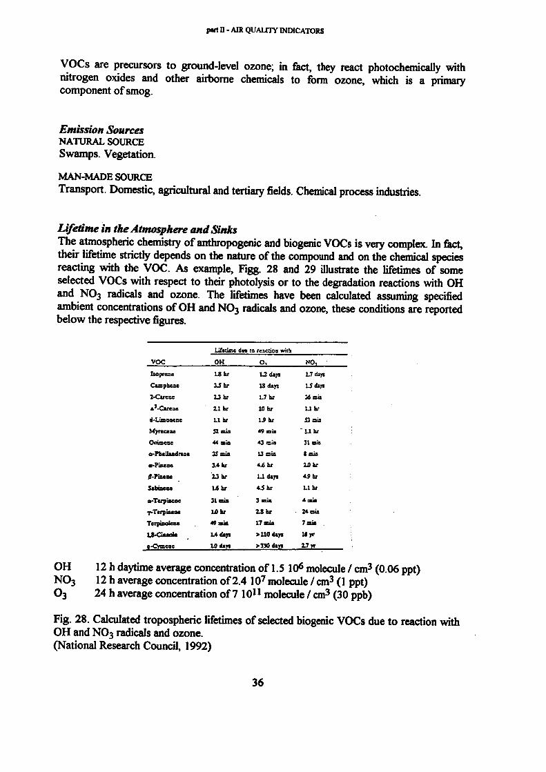
VOCs are precursors to ground-level ozone; in fact, they react photochemically with nitrogen oxides and other airborne chemicals to form ozone, which is a primary component of smog.

Emission Sources NATURAL SOURCE

Swamps. Vegetation.

MAN-MADE SOURCE

Transport. Domestic, agricultural and tertiary fields. Chemical process industries.

Lifetime in the Atmosphere and Sinks

The atmospheric chemistry of anthropogenic and biogenic VOCs is very complex. In fact, their lifetime strictly depends on the nature of the compound and on the chemical species reacting with the VOC. As example, Figg. 28 and 29 illustrate the lifetimes of some selected VOCs with respect to their photolysis or to the degradation reactions with OH and NO3 radicals and ozone. The lifetimes have been calculated assuming specified ambient concentrations of OH and NO3 radicals and ozone, these conditions are reported below the respective figures.

VOC

Isoprene

Casjpbeae

2-Careoe

i '-Cnene

d-Limoaene

Myreceae

Ocimeae

a-FheUaadrese

a-Pinese

0-Piaeae

Sabine«

α-Terp ¡nene

γ-Terpiaeae

Terpisolcae

1,8-Cneole

S-Cymeae

Lifetine due to reaction with

OH

LSbr

IS b

13 hr

l l a r

U h r

52 aun

44 aia

35 aua

3.4 hr

13 hr

1.6 hr

31 mia

UJhr

49 mia

» d t p

tO divi

O,

1.2 days

IS days

1.7 ai

IO or

1.9 hr

49 asia

43 s i a

13 s i a

4.6 hi

1.1 days

4 j a r

3 aua

I S h r

17 sua

> 110 days

> 330 davs

NO,

Udayi

lo days

36 mia

U h r

53 aia

' U h r

31 aia

t aia

10 hr

44 or

U h r

i ain

24 aia

7 min .

Myr

17 yr

OH 12 h daytime average concentration of 1.5 106 molecule / cm3 (0.06 ppt) NO3 12 h average concentration of 2.4 107 molecule / cm3 (1 ppt) O3 24 h average concentration of 7 1011 molecule / cm3 (30 ppb)

Fig. 28. Calculated tropospheric lifetimes of selected biogenic VOCs due to reaction with OH and NO3 radicals and ozone. (National Research Council, 1992)

36


voc Methane

Ethane

Propase

n-Butane

π-Octane

Ethene

Propeae

Isoprene

o-Pinene

Acetylene

Formaldehyde

Aeetaldehyde

Acetone

Methyl ethyl ketone

Methylglyoxal

Methanol

Ethanol

Methyl r-butyl ether

Benzene

Toulene

m-Xvleae

Lifetime due to reaction wich

OH

-12 years.

60 days

13 days

6.1 days

IS days

1.8 days

7.0 hours

1.8 hours

3.4 hours

19 days

1.6 days

1.0 days

68 days

13.4 days

10.8 hours

17 days

4.7 days

5.5 days

12-5 days

16 days

7.8 hours

NO,

> 120 years

> 12 years

>25 years

- 2 J years

260 days

225 days

4.9 days

50 min

5 min

a2_5 years

77 days

17 days e

c

c

>77days

>51days e

>6 years

1.9 years

200 days

0-, br

> 4,500 years

> 4,500 years

> 4,500 years

> 4,500 years

>4,500 years

9.7 days

1.5 days

1.2 days

1.0 days

5.8 years

>4J years

>4.5 years 4 hours

>4J years 15 days

><J years

>4J years 2 hours e

e

c

>4_5 years

>4J years

>4J years

OH 12 h average concentration of 1.5 106 molecule / cm3 (0,06 ppt) NO3 12 h average concentration of 5 108 molecule / cm3 (20 ppt) O3 24 h average concentration of 7 1011 molecule / cm3 (28 ppb)

c expected to be of negligible importance

Fig. 29. Calculated tropospheric lifetimes of selected anthropogenic VOCs due to photolysis and reaction with OH and NO3 radicals and ozone. (National Research Council, 1992)

Local Effects Photochemical Smog

37


2.5 HEAVY METALS AND THEIR COMPOUNDS

Definition and General Concepts The most important heavy metals in air quality assessment are the following:

ARSENIC As CADMIUM Cd CHROMIUM Cr COPPER Cu LEAD Pb MERCURY Hg NICKEL Ni ZINC Zn

Although they can be produced by natural phenomena, most of them come from anthropogenic activities. In fact, in particular As, Cd, Cu, Ni, Pb and Zn are released with the emissions of industrial plants. Moreover it is useful to point out that gasoline, containing tetraethyllead as anti-knock, is still widely used.

Heavy metals are seriously dangerous because of their potential ecological risk of biological build-up along the food chain. In fact, heavy metals can pass upwards to the next and subsequent level of the trophic pyramid; in this way, they bioconcentrate and become more and more toxic in those animals, including man, that occupy positions at the apex.

Emission Sources NATURAL SOURCE C rust al rock and soil. Vegetation. Volcanoes. Wildfires.

MAN-MADE SOURCES Industrial processes. Transport. Wastes. Combustion of wastes, fossil fuel and biomass.

Effects on Human Health Heavy metals are very toxic for man. Of course, effects depend on the heavy metals involved. For instance, the ingestion or absorption of lead over a prolonged period of time causes plumbism which is a lead poisoning characterised by colic, brain disease, anemia and inflammation of peripheral nerves. Heavy metals also may have both teratogenic and carcinogenic effects.

Effects on Vegetation Heavy metals come from the atmosphere with deposition. First, they accumulate in the canopy. Then, although some passes to the soil through litter fall, a considerable amount of heavy metals remains in the plant in the bark of the branches and stem. This accumulation leads to plant injuries which show as foliar and baric necroses.

38


2.6 SUSPENDED PARTICULATE

Definition and General Concepts The term Suspended Particulate (SP) indicates a mixture of organic and inorganic substances of varying size and composition which are present in atmosphere as little solid particles or volatile liquid drops The size is variable, but most particles belongs to the range 2 -90 urn. The measurement of the aerodynamic diameter defines two principal categories:

COARSE particles with aerodynamic diameter > 2.5 um FINE particles with aerodynamic diameter < 2.5 μιη

The composition of the SP depends on its origin. It may contain earth crostai particles, dust from cities and industries, materials produced by combustion and re-condensed vapours. The particles may include heavy metals such as lead or arsenic, heavy hydrocarbons, amianthus and other toxic compounds. The final fate of SP is the return to the soil as dry or wet deposition

The SP content in the air expresses the atmospheric pollution (Fig. 30).

AIR QUALITY

NOT POLLUTED AIR

URBAN AREA

HEAVILY POLLUTED AREA

SP (μιη / m3)

10

200

2,000

Fig. 30. Content of SP in unpolluted air and in polluted air.

Emission Sources NATURAL SOURCES Volcanoes. Dust storms, such as transport of mineral particles from soil or organic particles (i.e. pollen) by means of the wind.

MAN-MADE SOURCES Power plants. Industrial processes. Motor vehicles. Domestic coal burning. Industrial incinerators.

For each kind of anthropogenic sources, Fig. 31 reports the most representative pollutants that are emitted into the atmosphere as particulate.

39


SOURCE

INDUSTRY

WASTE

TRANSPORT

COMBUSTION

AGRICULTURE

MOST REPRESENTATIVE GROUP

heavy metals (Zn, Cd, Cu, Pb, Cr, Hg), solvents (benzene, toluene, chloralkenes, chloralkanes), PCBs

hydrocarbons, phenols, heavy metals (Cd, Cr, Ni, Pb, Zn), PCBs

PAHs, hydrocarbons (ethylene, acetylene, toluene, xylene), heavy metals (Pb)

hydrocarbons (pentanes, hexanes, etc.), heavy metals (V, Ni, Mn, Pb), PAHs, polychlorodibenzodioxins, polychlorodibenzofuranes

hexachlorocyclohexane, DDTs, endosulphan, chlordane, dieldrin, oxaphene, methoxychloro, heptachlorepoxide

Fig. 31. Sources of pollutants and most representative particulate bound compounds. (Mosello R et al., 1993. Translated.)

Lifetime in the Atmosphere and Sinks Suspended Particulate returns to Earth with depositions. Particles are deposited either faster or slower according to their size (Guderian R, 1986), as shown in Fig. 32.

PARTICLES

Coarse particles

Medium particles

Fine particles

DIAMETER

> 10 urn

0.5-10 μιη

< 0.5 um

DEPOSITION

Rapid deposition

Slow deposition

Deposition velocity increases because of brownian phenomena

Fig. 32. Deposition velocity of particles as a function of their size.

Local Effects Damage to Construction Elements and Other Materials: soiling of materials for building, painted surfaces and fabrics. Visibility Reduction

40


Effects on Human Health SP particles are inhaled by man. They penetrate the respiratory apparatus and deposit in different tracts according to their size (from the extrathoracic tract to the respiratory bronchioles); in fact, the size of a particle influences the areas of the respiratory system which that particle is likely to affect (Fig. 33). SP causes deficits in pulmonary function and its toxicity depends on the components of the particles (i.e. lead, amianthus, heavy hydrocarbons).

80 -

? 60

| s

40 -

20 -

-

-

I ι

Pulmonary

Traeheo-bronchiil

ι I

•ν ^ - . _

τ

^

Alveolar /"

ι

Ι Ι

Ι ι /

ι / ι / ι /

Ι / Ι /

ι / / /

' ι /

»

\ \

Nasal /

Λ \ \

t ι t

ι ι ι \

ι W 0.01 ο.ο: 0.05 0.1 0.2

Panicle radius Cum) 0.5 i.O 2.0

Fig. 33. Fractional amount of particles of various size deposited in the different areas of the respiratory tract. (Brimblecombe P., 1986)

Effects on Vegetation The particles can be separated into inert and toxic. Inert particulate causes mainly physical effects on plants, whereas toxic particulate have both chemical and physiological effects depending on the toxicity of the components that constitute the particles.

41


2.7 CHLOROFLUOROCARBONS (CFCs)

Definition and General Concepts The term chlorofluorocarbons refers to a family of compounds derived from methane or higher carbon-content hydrocarbon molecules. A CFC forms by replacing all hydrogen atoms with chlorine or fluorine halogens. When bromine is used, the compounds are called halons. CFCs are liquid or gaseous products. They are used as aerosol spray propellants, refrigerants, solvents and plastic foaming agents. They accumulate in the atmosphere. In stratosphere, they react, with catalytic effect, to form highly reactive chlorine species which can electronically react with the ozone destroying it. The catalytic effect means that just one CFC molecule can destroy 20,000 - 30,000 molecules of 0 3 (Vismara R, 1988). For this reason, CFCs are involved in the depletion of the ozone layer. Fig. 34 shows the destruction mechanism of the stratospheric ozone because of the release of CF2CI2 in the environment.

Ozone absorbs UV light

CF2Cl2 + hv >- CI + CF;CI 50km 280 K 0 · 7torr

CI + CH4

O3 + CI ► CIO + 0 2 θ ' + CIO ► CI + O-, net O + Oy>O2 + 0 2

S , r a t o s P h " > W ^ d o w n O o Troposphere ^ » 3 0 0 n

CF,Ch release

rrr,

HCL

'Rain- '0-l5km Ra,rT 210K 70torr 5LV mmmmsp

Fig. 34. Destruction mechanism of the stratospheric ozone following the release of CF2Cl2 in the environment. (SamiullahY, 1990)

Because CFCs are strong absorbers of ER, they contribute to the greenhouse effect when they are in the lower atmosphere. In coming years, it is expected that production and emission of CFCs will be reduced as a result of the Montreal Protocol (Council Decision 88/540/EEC) and other international

42


policy agreements. For example, the Council Regulation EEC/594/91 reported the estimated ozone-depleting potentials for the CFCs and other compounds which are recognised to be substances that deplete the ozone layer (Fig. 35).

Emission Sources NATURAL SOURCES None.

MAN-MADE SOURCE Chemical industry: refrigeration and air conditioning, closed-cell and open-cell foams, aerosol propellant.

Lifetime in the Atmosphere and Sinks Mean residence time in the atmosphere (Wuebbles D.J. and Edmonds J., 1991):

CFCI3 (CFC-11) from 50 to 80 years CF2C12 (CFC-12) from HOto 130 years CFC12CF2C1 (CFC-113) ~0 years CF2C1CF3 (CFC-115) ~ 400 years

In the troposphere there are no significant losses; whereas in the stratosphere, CFCs photodissociate and react with oxygen atoms forming reactive chlorine compounds.

Global Effects Depletion of Ozone Layer Greenhouse Effect

Croup

Croup 1

Croup II

.

CFdj

CF2C32 C2F5CI3 CiNCIj

C2i'$a

CT3C1

c2ra5 C2F2CI4 C3FCI7 CiFtOí C&Øi C5F4CI4 C3F5C13 Cír^Crí

cjira

Substance

(CFC-11) (CFC-12) (CFC-113) (CFC-I IO (CFC-1 IS)

(CFC-13) (CFC-111) (CFC-112) (CFC-211) (CFC-212) (CFC-213) (CFC-214) (CFC-21S) CFC-216) (CFC-217)

Ozone-depleting potential

LO LB 0»

u> 0.Í

ID ID 1.0 LO LO U) LO LO LO IJO

continued

43


Croup

Croup ill

Croup IV

Croup V

Croup VI

Croup VI

'

Substance

Cf2UrCI

CKjür

C2F4UT2

ecu

C2H3CI32

CHFCI2

CHF2a

CH2FO

C2HFCI4

C2HF2CIJ

C2HF3a2

C2HF4CI

C2H2FÛ3

C2II2H2CI2

C2I frâ

C2I13F02

Ç2H3F2CI

C2I14FO

C3IIF06

cînâs C3IIF3CL4

CÛMC^

C311F5CI2

C31 ιΐ'όα C3ii2Fa5

C3ll2ls2CM C3H2lf3Cl3 C3H2F4CI2 C3II2I-5O C3II3FCI4 c3 i 131-203 C3II3H3CI2 C3II3IMCI C3H4FCI3 C3lHI!2d2 C3lUI'3a C3H5102 C3H5l'2a C3II6IO

(halon-1211) Chalón· 1301) (halon-2402)

(carbon tetrachloride)

(1,1,1 -1 r ich 1 oroe iha ne)

CHCFC-2I) (HCFC-22) (HCTC-31) (HCKM21) (HCFC-122) CHOC-123) CHC1-C-124) (HCFC-131)

(HCFC-132) (IICFC-133) (IICI:C-141> (l ICFC-142) (wcrc-151) (nafc-22i) (Iia:C-222) (HafC-223) QICFC-224) (IICFC-225) (1 ICTC-226) (IICFC-231) (lia-C-232) (lia-C-233) (I1C1-C-234) (IICFC-235) (HCFC-241) (HCIC-242) (UOC-243) (na-c-244) •(MO-C-25I) (na-C-252) (uac-253) (IIŒC-26D (liaC-262) 0lQ"C-27n ..

Oionc-dcpleiing potential

3.0 10.0 6.0

1.1

0.1

·;..

Fig. 35. Substances that deplete the ozone layer. (Council Regulation EEC/594/91)

44


2.8 CARCINOGENIC SUBSTANCES

Definition and General Concepts "Carcinogenic substances" means all those substances and preparations which has been proved to possess carcinogenic properties via the air. PAHs are the most representative group. They are organic compounds with two or more benzene rings. There are many PAHs, of which the best known is benzo[a]pyrene. They derive from incomplete combustion of organic materials and from evaporation in gasoline-powered motors. Because of this, the PAH concentration in urban centres is 1,000 times greater than that measured in wooded areas. Some PAHs, deriving from combustion, which are recognised to be carcinogenic are:

benzo[a]pyrene 3 -met hy I cholant hr ene dibenzo[c,g]carbazole benzo[cb]fluoranthene benzo[c]phenananthrene

Emission Sources NATURAL SOURCE Wildfires.

MAN-MADE SOURCES Combustion of wastes, fossil fuel, biomass. Motor vehicles.

Effects on Human Health PAHs irritate eyes and interfere with the respiratory processes. It is recognised that PAHs are carcinogenic.

2.9 OZONE (0 3 )

Definition and General Concepts Ozone is a blue gas with a typical odour of garlic. It is a reactive oxidant gas which is, in the atmosphere, created and destroyed at the same time. In fact, it forms from 0 2 and atomic oxygen (produced by solar photodissociation of N0 2 ) and is simultaneously demolished by reaction with atomic oxygen or stratospheric NOx-components and by photodissociation. Because these two processes are in photochemical equilibrium, the ozone concentration remains stationary. This equilibrium can be disturbed by some anthropogenic gases such as CFCs. In the stratosphere, where most ozone is found, it has a crucial role because it adsorbs the UV radiation (0.2 - 0.3 um) emitted by the sun, which damages plant and animal life. It is noticed that a significant weakening of the stratospheric ozone layer could lead to the increase of instances of skin cancer in the human population.

45


On the other hand, in the troposphere, high concentrations of ozone may be harmful for man, animals and plants. Besides, because the tropospheric ozone is a greenhouse gas which can trap the radiation emitted by the earth, it is reasonable to suppose that an increase of the tropospheric ozone concentration could contribute to a warming of the terrestrial surface. It is for this reason that ozone is supposed to be involved in "global change", where global change means changes in climate and changes in atmospheric chemistry.

Unit Conversion factor (WHO, 1987): 1 ppm = 2 mg / m3

Emission Sources NATURAL SOURCE Atmospheric processes.

MAN-MADE SOURCES Indirectly by chemical reactions of gaseous emissions of plants (in fact, 0 3 is a secondary pollutant).

Lifetime in the Atmosphere and Sinks Mean residence time in the atmosphere: ~ 1 week (Beilke S., 1987). Sinks are the losses due to chemical reactions with atmospheric compounds and to deposition on earth.

Local Effects Damage to Construction Elements and Other Materials: see Fig. 36. Photochemical Smog

MATERIAL ATTACKED

RUBBER and ELASTOMERS

NATURAL and SYNTHETIC FABRICS

DYES

DAMAGE

weakening and breaking

weakening

fading

Fig. 36. Effects of ozone on some materials. (Vismara R, 1988. Translated and modified.)

46


Global Effects Greenhouse Effect

Effects on Human Health Exposure to 0 3 may cause a decrease in pulmonary function, irritation to eyes, nose and throat. Asthmatic crises, in predisposed subjects, have also been reported. Irritation to sense organs has been noted in subjects exposed to concentrations around 0.1 - 0.15 ppm (Vismara R, 1988).

To protect public health, WHO guidelines suggest the following maximum values for 0 3 (WHO, 1987):

from 150 to 200 μg / m3 (from 0.076 to 0.1 ppm) for an exposure time of 1 hour from 100 to 120 μg / m3 (from 0.05 to 0.06 ppm) for an exposure time of 8 hours

Effects on Vegetation Vegetation absorbs ozone via the stornata by the gas exchange process. These visible injuries have been observed: premature senescence and defoliation, leaf-yellowing, necrosis. Some metabolic processes are also damaged; in fact, it has been noted that the rate of photosynthesis may decrease. The presence of S0 2 increases the negative effect of O3 on the leaves. Species sensitive to ozone are: alfalfa, barley, bean, oats, onion, maize, apple-tree, vine, tobacco, tomato, spinach, poplar, maple, white pine-tree, yellow pine-tree (Vismara R, 1988). Moreover, Fig. 37 lists other woody species grouped according to their degree of sensitivity to ozone.

WHO guidelines report the following maximum values for O3 in order to protect vegetation (WHO, 1987):

200 μg / m3 for an exposure time of 1 hour 65 pg / m3 for an exposure time of 24 hour 60 pg / m3 during the growing season ( 100 days)

47


VERY SENSITIVE SPECIES

Ailanthus altissima

Cotoneaster divaricatus

Cotonea ster horìzontalis

Gleditsia triacanthos inermis

Juglans regia

Larix decidua

Ligustrum velgare var. pyramidae

Liriodendron tulipifera

Pinus nigra

Platanus occidentalis

Populus maximowiczii χ trichocarpa Sorbus aucuparia

Spiraea χ vanhouttei

Symphoricarpos albus

SENSITIVE SPECIES

Acernegundo

Forsythia χ intermedia

'Lynwood Gold'

Larix kaempferi

Ligustrum vulgare

Liquidambar styraciflua

Philadelphus coronarius

Pinus strobus

Pinus sylvestris

Sy ringa vulgaris

Tsuga canadensis

LESS SENSITIVE SPECIES

Abies concolor Acer platonoides

Bet ula pendula

Buxus sempervirens

Fagus sylvatica

Ilex aquifolium

Ilex crenata

Juglans nigra

Picea abies

Picea pungens

Pieries japónica Pseudotsuga menziesii

Quercus robur Quercus rubra

Robinia pseudoacacia

Sophora Japónica

Thuja occidentalis

Tilia americana

Tilia cordata

Viburnum χ burkwoodii

Viburnum cariesii

Fig. 37. Relative sensitivity of woody species to ozone. (Krause G.H.M., 1988)

48

part ΠΙ - INDICATOR REFERENCE VALUES ACCORDING TO REGULATIONS AND GUIDELINES

3 INDICATOR REFERENCE VALUES ACCORDING TO REGULATIONS AND GUIDELINES

The reference values for air quality indicators have been defined by means of legislation and guidelines. This chapter has therefore been divided into two different sections: Regulations and Guidelines. The former reports the reference values taken from EU Directives and Italian legislation. The latter uses WHO guidelines to draw out the indicator reference values.

3.1 REGULATIONS

European Union regulations have here been considered as the starting point; then, the Italian legislation has been examined, to see how Italy has applied the EU Directives. As already mentioned in section 1.2.7, two different series of laws have been produced: the former concerns air quality monitoring and the later concerns the control of pollutant emissions. For this reason, two parts have been separated: Air Quality and Emissions from Industrial Plants.

3.1.1 AIR QUALITY

The following regulations refer to the safeguard of air quality. With this aim, they fix reference values, as Limit Values and Guide Values, for air pollutants.

The first EU Directive produced to protect air quality is Directive 80/779/EEC. It establishes the Guide Values and Limit Values for sulphur dioxide and suspended particulate in the atmosphere (Figg. 38, 39,40,41 and 42).

REFERENCE PERIOD

Year

24 hours

GUIDE VALUE FOR SULPHUR DIOXIDE

40 to 60 arithmetic mean of daily mean values taken throughout the year

100 to 150 daily mean value

Fig. 38. Guide Values for sulphur dioxide expressed in pg / m3. (Directive 80/779/EEC)

49

part III - INDICATOR REFERENCE VALUES ACCORDING TO REGULATIONS AND GUIDELINES

REFERENCE PERIOD

Year

24 hours

GUIDE VALUE FOR SUSPENDED PARTICULATE

40 to 60 arithmetic mean of daily mean values

taken throughout the year

100 to 150 daily mean value

Fig. 39. Guide Values for suspended particulate (measured by black-smoke method) expressed in μg / m3. (Directive 80/779/EEC)

REFERENCE PERIOD

Year

Winter (1 October to 31 March)

Year (made up of units of

measuring periods of 24 hours)

LIMIT VALUE FOR SUSPENDED PARTICULATE

80 median of daily mean values


130 median of daily mean values taken throughout the winter

250 (·) 98th percentile of all daily mean values


(*) this value must not be exceeded for more than three consecutive days

Fig. 40. Limit Values for suspended particulate (measured by black-smoke method) expressed in pg / m3. (Directive 80/779/EEC)

50


REFERENCE PERIOD



Winter (1 October to 31 March)



LIMIT VALUE FOR SULPHUR DIOXIDE







250 (*) 98th percentile of all daily mean

values taken throughout the year



ASSOCIATED VALUE FOR SUSPENDED PARTICULATE

>40 median of daily mean values


¿40 median of daily mean values


>60 median of daily mean values taken throughout the winter

¿60 median of daily mean values taken throughout the winter

>150 98 th percentile of all daily mean


¿150 98 th percentile of all daily mean



Fig. 41. Limit Values for sulphur dioxide with the associated values for suspended particulate (measured by black-smoke method) expressed in pg / m3. (Directive 80/779/EEC)

51


j REFERENCE PERIOD

Year

j Winter (1 October to 31 March)



LIMIT VALUE FOR SULPHUR DIOXIDE






180 meciian of daily mean values taken throughout the winter

250 (*) 98<h percentile of all daily mean




ASSOCIATED VALUE FOR SUSPENDED PARTICULATE

>150 median of daily mean values


¿150 median of daily mean values


>200 median of daily mean values taken throughout the winter

¿200 median of daily mean values taken throughout the winter

>350 98th percentile of all daily mean


¿350 98th percentile of all daily mean



Fig. 42. Limit Values for sulphur dioxide with the associated values for suspended particulate (measured by gravimetric method) expressed in pg / m3. (Directive 80/779/EEC)

Regarding heavy metals, Directive 82/884/EEC fixes a Limit Value for lead in the air specifically in order to help protect human beings against the effects of lead in the environment. This value is the following:

LIMIT VALUE OF LEAD IN AIR 2 pg / m3 expressed as annual mean concentration

The Italian legislation complied to the EU Directives on air quality. In fact, DPCM No. 30, 28/03/1983 has established the maximum limits of acceptability of the concentrations and maximum exposure limits for air pollutants in the outside environment (Fig. 43). Besides, this decree also gives the Limit Value of the concentration in the air of

52

part lil - INDICATOR REFERENCE VALUES ACCORDING TO REGULATIONS AND GUIDELINES

hydrocarbons because it is known that they are the precursors of the pollutants considered in Fig. 43 (Fig. 44).

POLLUTANT

SULPHUR DIOXIDE expressed as SO,

NITROGEN DIOXIDE expressed as NO,

OZONE expressed as O,

CARBON MONOXIDE expressed as CO

LEAD

FLUORINE

SUSPENDED PARTICULATE

LIMIT VALUE

Median of the average 24 h concentration levels recorded throughout the entire year

98th percentile of the average 24 h concentration levels recorded throughout the entire year

Average 1 h concentration level not to be exceeded more than once a day

Average 1 h concentration level not to be reached more than once a month

Average 8 h concentration level


Arithmetical average of the average 24 h concentration levels recorded over 1 year


Average of the average 24 h concentration levels recorded over 1 month

Arithmetical average of all the average 24 h concentration levels recorded over a year

95th percentile of all the average 24 h concentration levels recorded over a year

80 μς / m3

250 ug / m3

200 ug / m3

200 μg / m3

10 mg/m 3

40 mg / m3

2 μg / m3

20 ug / m3

10μg/m3

150μg/m3

300 μς / m3

Fig. 43. Limit Value of acceptability of the concentrations and maximum exposure limits for air pollutants outside. (DPCM No. 30, 28/03/1983. Translated.)

53


PRECURSOR

TOTAL HYDROCARBONS excluding methane

expressed as C

LIMIT VALUE

Average consecutive 3 h concentration levels during

periods of the day to be specified according to the

various different areas by the appropriate regional

authorities

200 ug / m3

CONDITIONS FOR THE LIMIT VALUE

TO BE VALID

To be adopted only in areas and periods of the

year when the limit values for ozone have been

significantly exceeded

Fig. 44. Limit Value of the concentrations in air of precursors of the pollutants shown in Fig. 43, to adopt in certain conditions. (DPCM No. 30, 28/03/1983. Translated.)

Directive 85/203/EEC furnishes the air quality standards for nitrogen dioxide as Limit Value and Guide Value (Figg. 45 and 46).

REFERENCE PERIOD

Year

LIMIT VALUE FOR NITROGEN DIOXIDE

200 98th percentile calculated from the mean values per hour or period

of less than an hour recorded throughout the year

Fig. 45. Limit Value for nitrogen dioxide expressed in pg / m3. (Directive 85/203/EEC)

REFERENCE PERIOD

Year

GUIDE VALUE FOR NITROGEN DIOXIDE

50 50th percentile calculated from the mean values per hour or per period of less

than an hour recorded throughout the year

135 98th percentile calculated from the mean values per hour or per period of less

than an hour recorded throughout the year

Fig. 46. Guide Values for nitrogen dioxide expressed in pg / m3. (Directive 85/203/EEC)

54


In Italy DPR No. 203, 24/05/1988 was produced with the purpose of implementing EU Directives No. 80/779, 82/884, 84/360 and 85/203. It determines the Guide Values for sulphur dioxide, nitrogen dioxide and suspended particulate and the Limit Values for sulphur dioxide and nitrogen dioxide (Figg. 47 and 48).

POLLUTANT

\ SULPHUR DIOXIDE SO,

NITROGEN DIOXIDE NO,


(measured by the black-smoke method)

GUIDE VALUE

Arithmetical average of the average 24 h concentration levels recorded over 1 year: from 40 to 60 μ9 / m3

Average 24 h value: from 100 to 150 μς / m3

50th percentile of the average 1 h concentration levels recorded throughout the entire year 50 ug / m3

98th percentile of the average 1 h concentration levels recorded throughout the entire year 135μg/m3

Arithmetical average of the average 24 h concentration levels recorded over 1 year from 40 to 60 μg equivalent black smoke / m3

Average 24 h value: from 100 to 150 μg equivalent black smoke / m3

REFERENCE PERIOD

01-04/31-03

0 a.m. /12 p.m. of every day

01-01/31-12

01-01/31-12

01-04/31-03

0 a.m. /24 p.m. of every day

Fig. 47. Guide Values of sulphur dioxide, nitrogen dioxide and suspended particulate for air quality. (DPR No. 203, 24/05/1988. Translated.)

55


POLLUTANT

', SULPHUR DIOXIDE SO,

! NITROGEN DIOXIDE NO,

UMIT VALUE

Median of the average 24 h concentration levels recorded throughout the entire year: 80 μg / m3

98th percentile of the average 24 h concentration levels recorded throughout the entire year 250 ug / m3

Median of the average concentration levels recorded during the winter: 130pg/m3

98th percentile of the average 1 h concentration levels recorded throughout the entire year 200 μg / m3

REFERENCE PERIOD

01-04/31-03

01-04/31-03

01-10/31-03

01-01/31-12

Fig. 48. Limit Values of sulphur dioxide and nitrogen dioxide for air quality. (DPR No. 203, 24/05/1988. Translated.)

The aim of DMA 12/11/1992 is to control atmospheric pollution in large urban zones. This decree fixes the limits of the Attention Level and Alarm Level for atmospheric pollutants (Fig. 49). The attention level and alarm level define the concentration of the pollutant which determines the Attention State and Alarm State respectively. The attention state is a situation that, if persisting, leads to the alarm state. In turn, the alarm state, if persisting, leads to potential exceeding of the maximum limits of acceptability (fixed by DPCM No. 30, 28/03/1983), which is risky for the general population.

56


POLLUTANT

SULPHUR DIOXIDE ug / m3

(daily average)

TOTAL SUSPENDED PARTICLES ug/m3

(daily average)

NITROGEN DIOXIDE ug / m3

(average 1 h value)

CARBON MONOXIDE mg / m3

(average 1 h value)

OZONE ug/m3

(average 1 h value)

ATTENTION LEVEL

125 Π

90 (*)

200

15

120

ALARM LEVEL

250 C)

180 (*)

400

30

240

(*) jointly in the same monitoring station

Fig. 49. Attention levels and alarm levels for air pollutants in large urban zones. (DMA 12/11/1992. Translated.)

The still temporary Directive 92/72/EEC closes the regulations concerning the air quality monitoring. It establishes the thresholds for ozone concentrations in the air according to four specific purposes (Fig. 50).

PURPOSES

HEALTH PROTECTION

VEGETATION PROTECTION

POPULATION INFORMATION

POPULATION WARNING

THRESHOLDS FOR OZONE CONCENTRATIONS

100 ug / m3 for the mean value over 8 hours

200 ug / m3 for the mean value over 1 hour 65 pg / m3 for the mean value over 24 hours

180 ug / m3 for the mean value over 1 hour

360 ug / m3 for the mean value over 1 hour

Fig. 50. Thresholds for ozone concentrations in the air. (Directive 92/72/EEC)

57


3.1.2 EMISSIONS FROM INDUSTRIAL PLANTS

Six categories of industrial plants were considered in Directive 84/360/EEC, they are the following:

(1) ENERGY INDUSTRY • Coke ovens • Oil refineries (excluding undertakings manufacturing only lubricants from crude oil) • Coal gasification and liquefaction plants • Thermal power stations (excluding nuclear power stations) and other combustion

installations with a nominal heat output of more than 50 MW

(2) PRODUCTION AND PROCESSING OF METALS • Roasting and sintering plants with a capacity of more than 1,000 tonnes of metal ore

per year • Integrated plants for the production of pig iron and crude steel • Ferrous metal foundries having melting installations with a total capacity of over 5

tonnes • Plants for the production and melting of non-metals having a total capacity of over 1

tonne for heavy metals or 0.5 tonne for light metals

(3) MANUFACTURE OF NON-METALLIC MINERAL PRODUCTS • Plants for the production of cement and rotary kiln lime production • Plants for the production and processing of asbestos and manufacture of asbestos-

based products • Plants for the manufacture of glass fibre or mineral fibre • Plants for the production of glass (ordinary and special) with a capacity of more than

5,000 tonnes per year • Plants for the manufacture of coarse ceramics notably refractory bricks, stoneware

pipes, facing and floor bricks and roof tiles

(4) CHEMICAL INDUSTRY • Chemical plants for the production of olefins, derivatives of olefins, monomers and

polymers • Chemical plants for the manufacture of other organic intermediate products • Plants for the manufacture of basic inorganic chemicals

(5) WASTE DISPOSAL • Plants for the disposal of toxic and dangerous waste by incineration • Plants for the treatment by incineration of other solid and liquid waste

(6) OTHER INDUSTRIES • Plants for the manufacture of paper pulp by chemical methods with a production

capacity of 25,000 tonnes or more per year

58


Following this directive, Directive 88/609/EEC was produced. It must be applied to existing and new combustion plants with a thermal input equal or greater than 50 MW independent of the type of fuel. Regarding new plants, this directive establishes the limits of the emission of sulphur dioxide, nitrogen oxides and dust according to the type of fuel used (Figg. 51, 52, 53, 54 and 55).

200 -

SOLID FUELS

100 200 300 400 500 600 MWth

Fig. 51. Sulphur dioxide emission limit values for new plants which use solid fuel. (Directive 88/609/EEC)

TYPE OF FUEL

Gaseous fuels in general

Liquefied gas

Low calorific gases from gasification of refinery residues, coke oven gas, blast-furnace gas

LIMIT VALUES (mg / Nm*)

35

5

800

Fig. 52. Sulphur dioxide emission limit values for new plants which use gaseous fuel. (Directive 88/609/EEC)

59

part ΙΠ - INDICATOR REFERENCE VALUES ACCORDING TO REGULATIONS AND GUIDELINES

m g S 0 2 / N m 3

1700

1600

1500

1400

1300

1200

1100

1000

900

800

700

eoo

500

400

1 1 1 1

I LIQUID FUELS

ι ι t^JLmn

100 200 300 400 500 600 MWth

Fig. 53. Sulphur dioxide emission limit values for new plants which use liquid fuel. (Directive 88/609/EEC)

TYPE OF FUEL

Solid in general

Solid with less than 10% volatile compounds

Liquid

Gaseous

LIMIT VALUES (mg / Nm*)

650

1,300

450

350

Fig. 54. Nitrogen oxides emission limit values for new plants according to the type of fuel used. (Directive 88/609/EEC)

60


TYPE OF FUEL

Solid

Liquid (*)

Gaseous

THERMAL CAPACITY

(MWth)

¿500

¿500

all plants

all plants

EMISSION LIMIT VALUES

(mg / Nm3)

50

100

50

5 as rule

10 for blast furnace gas

50 for gases produced by the steel industry,

which can be used elsewhere

(*) a limit value of 100 mg / Nm3 may be applied to plants with a capacity of less than 500 MWth burning liquid fuel with an ash content of more than 0.06%

Fig. 55. Dust emission limit values for new plants according to the type of fuel used. (Directive 88/609/EEC)

In Italy, Directive 88/609/EEC was implemented in the two decrees DMA 08/05/1989 and DMA 12/07/1990. The former concerns new large combustion plants, whereas the latter concerns existing industrial plants. Because this paper is focused on the EIA, only the aspect relative to new plants is subject of this work, therefore only DMA 08/05/1989 has been examined. This decree reports the emission limit values for sulphur dioxide, nitrogen oxides and dust according to the type of fuel used (Fig. 56, 57, 58, 59, 60,61 and 62).

61


mg S 0 2 / N m 3

SOLID FUELS

100 200 300 400 500 600 MWth

Fig. 56. Sulphur dioxide emission limit values for new plants which use solid fuel. (DMA 08/05/1989)

m g S O , / N m 3

1700

1000

1S00

1400

1300

1200

1100

1000

900

soo 700

«00

soo

—

— — — —

i LIQUID FUELS

\ \

\ \

\ \

\ \

\ \

\

100 200 300 400 S00 • 00 MWth

Fig. 57. Sulphur dioxide emission limit values for new plants which use liquid fuel. (DMA 08/05/1989)

62


TYPE OF FUEL

Gaseous fuels in general

Liquefied gas

Low calorific gases from gasification of refinery residue, coke oven gas, blast-furnace gas

LIMIT VALUE (mg / Nm3)

35

5

800

Fig. 58. Sulphur dioxide emission limit values for new plants which use gaseous fuel. (DMA 08/05/1989. Translated.)

mgMO./Nm» Ϊ Π Γ

600

500

400

300

200

100

1 1 , 1 1 1 1

SOUD FUELS

1 1 1 1

100 200 300 400 500 600 MWth

Fig. 59. Nitrogen oxides emission limit values for new plants which use solid fuel. (DMA 08/05/1989)

63


mgNOx/Nm3

500

400

300

200

100

—

_ l L 1_ .!_. 1 t 1

UQUID FUELS

■ ■ » '

100 200 300 400 500 600 MWth

Fig. 60. Nitrogen oxides emission limit values for new plants which use liquid fuel. (DMA 08/05/1989)

mg NOx / Nm3

400 —

300 —

200

100 —

—

—

~̂

1 1 1 J ' ■ '

GASEOUS FUELS

I I I I

100 20O 300 400 500 600 MWth

Fig. 61. Nitrogen oxides emission limit values for new plants which use gaseous fuel. (DMA 08/05/1989)

64

part IH - INDICATOR REFERENCE VALUES ACCORDING TO REGULATIONS AND GUIDELINES

TYPE OF FUEL

liquid and solid

gaseous

THERMAL CAPACITY (MWth)

¿50

¿50

LIMIT VALUE (mg / Nm3)

50

5 as a rule

10 for blast furnace gas

50 for gases produced by the steel industry which can be used elsewhere

Fig. 62. Dust emission limit values for new plants according to the type of fuel used. (DMA 08/05/1989. Translated.)

Directive 89/369/EEC concerns new municipal waste incineration plants. The air pollutants considered are dust, heavy metals, hydrochloric acid, hydrofluoric acid and sulphur dioxide. For each of these pollutants, the emission limit values are specified according to the nominal capacity of the plant (Fig. 63).

POLLUTANT

Total dust

Heavy metals: - Pb + Cr + Cu + Mn -Ni +As - Cd and Hg

Hydrochloric acid (HCl)

Hydrofluoric acid (HF)

Sulphur dioxide (SO,)

less than 1 tonne / h

200

-

250

-

-

1 tonne / h or more but less than 3 tonne* / h

100

5 1

0.2

100

4

300

3 tonnes / h or more

30

5 1

0.2

50

2

300

Fig. 63. Emission limit values for dust, heavy metals, hydrochloric acid, hydrofluoric acid and sulphur dioxide (expressed in mg / Nm3) as a function of the nominal capacity of the incineration plant. (Directive 89/369/EEC)

65


3.2 GUIDELINES

WHO guidelines have defined reference values for the most crucial air pollutants (WHO, 1987). These guidelines are the result of experimental observations of the damage to the environment due to the exposure to atmospheric pollutants. The reference values reported represent the pollutant level, combined with the relative exposure time, at which no adverse effects are expected. In particular, the maximum concentration of pollutant that seems not to be a danger for man and plants has been evaluated; so two sections have been separated: Human Health and Vegetation. The guidelines for preserving human health have been located in the former, whereas the latter contains the guidelines for protecting plant life. The reference values, reported below, have already been given for each pollutant in PART II under the points Effects on Human Health and Effects on Vegetation. They also have been summarised here in tables to give a whole overview.

3.2.1 HUMAN HEALTH

To protect human health from air pollution, WHO has suggested guideline values for some air pollutants (WHO, 1987). These values are indicated as maximum concentration level of pollutant with exposure time. They are summarised in Fig. 64.

3.2.2 VEGETATION

WHO also has drawn up guidelines for the protection of vegetation (WHO, 1987). Like the guidelines to protect human health given below, these values express the maximum concentration level of pollutant joined with the exposure time. They are summed up in Fig. 65.

66

part UI - INDICATOR REFERENCE VALUES ACCORDING TO REGULATIONS AND GUIDELINES

POLLUTANT

SULPHUR DIOXIDE

SO,

NITROGEN DIOXIDE

NO,

CARBON MONOXIDE

CO


OZONE

REFERENCE VALUE

500 ug / m3

350 μ9 / m3

1 2 5 μ g / m 3 (1)

5 0 μ g / m 3 (1)

400 μg / m 3 (0.21 ppm)

150 μ9 / m3 (0.08 ppm)

100 m g / m 3

60 mg / m3 (50 ppm)

30 m g / m 3 (25 ppm)

10 mg / m3 (10 ppm)

1 2 5 μ g / m 3 (1) (2)

50 u g / m 3 (1) (2)

from 150 to 200 μς / m 3 (from 0.076 to 0.1 ppm)

from 100 to 120 μ9 / m3 (from 0.05 to 0.06 ppm)

EXPOSURE TIME

10 minutes

1 h

24 h

1 year

1 h

24 h

15 minutes

30 minutes

1 h

8 h

24 h

1 year

1 h

8 h

(1) considered jointly

(2) measured by the black-smoke method

Fig. 64. Air quality WHO guidelines to protect human health.

67


POLLUTANT

SULPHUR DIOXIDE

SO,

NITROGEN DIOXIDE

NO,

OZONE

■ ■-■■

REFERENCE VALUE

30 μρ / m3

Annual average

100 ug/m3

24 h average

3 0 w / m3 (*)

Yearly average of 24 h means

95 rø /m3 (*)

4 h average

200 ug/m3

65 ug / m3

60 μg 1 m3

EXPOSURE TIME

1 year

24 h

1 year

4h

1h

24 h

growing season (100 day)

(*) in conditions of SO2 < 30 pg / m3 and O3 < 60 pg / m

3

Fig. 65. Air quality WHO guidelines to protect vegetation.

68

REFERENCES

REFERENCES

LEGISLATION AND GUIDELINES

COUNCIL DECISION 88/540/EEC. Council Decision of 14 October 1988 concerning the conclusion of the "Vienna Convention for the protection of the ozone layer and the Montreal Protocol on substances that deplete the ozone layer. Official Journal of the European Communities L 297, 30-10-1988: 8-28.

COUNCIL REGULATION EEC/594/91. Council Regulation of 4 March 1991 on substances that deplete the ozone layer. Official journal of the European Communities L 67, 14-03-1991:1-10.

DIRECTIVE 80/779/EEC. Council Directive of 15 July 1980 on air quality limit values and guide values for sulphur dioxide and suspended particulates. Official Journal of the European Communities L 229, 30-08-1980: 30-48.

DIRECTIVE 82/884/EEC. Council Directive of 3 December 1982 on a limit value for lead in the air. Official Journal ofthe European Communities L378, 31-12-1982: 15-19.

DIRECTIVE 84/360/EEC. Council Directive of 28 June 1984 on the combating of air pollution from industrial plants. Official Journal of the European Communities L 188, 16-07-1984: 20-25.

DIRECTTVE 85/203/EEC. Council Directive of 7 March 1985 on air quality standards for nitrogen dioxide. Official Journal of the European Communities L 87,27-03-1985: 1-7.

DIRECTIVE 85/337/EEC. Council Directive of 27 June 1985 on the assessment of the effects of certain public and private projects on the environment. Official Journal of the European Communities L 175, 05-07-1985: 40-48.

DIRECTIVE 88/609/EEC. Council Directive of 24 November 1988 on the limitation of emissions of certain pollutants into the air from large combustion plants. Official Journal of the European Communities L 336,07-12-1988: 1-13.

DIRECTIVE 89/369/EEC. Council Directive of 8 June 1989 on the prevention of air pollution from new municipal waste incineration plants. Official Journal of the European Communities!. 163,14-06-1989: 32-36.

DIRECTIVE 92/72/EEC. Council Directive of 21 September 1992 on air pollution by ozone. Official Journal of the European Communities L 297,13-10-1992.

DMA 08/05/1989. Limitazione delle emissioni nell'atmosfera di taluni inquinanti originati dai grandi impianti di combustione (Limitation of the emissions into the atmosphere of certain pollutants from large combustion plants). Gazzetta Ufficiale della Repubblica Italianako. 124, 30-05-1989: 40-52.

69

REFERENCES

DMA 12/11/1992. Criteri generali per la prevenzione dell'inquinamento atmosferico nelle

grandi zone urbane e disposizioni per il miglioramento della qualità dell'aria (General

criteria preventing atmospheric pollution in large urban zones and provisions for the

improving of air quality). Gazzetta Ufficiale della Repubblica Italiana No. 272, 18-11-

1992: 15-29.

DPCM No. 30, 28/03/1983. Limiti massimi di accettabilità delle concentrazioni e di

esposizione relativi ad inquinanti dell'aria nell'ambiente estemo (Maximum limit values of

acceptability of the concentrations and exposure for air pollutants outside). Supplemento

Ordinario della Gazzetta Ufficiale della Repubblica Italiana No. 145, 28-05-1983: 3-

21.

DPCM No. 377,10/08/1988. Regolamentazione delle pronunce di compatibilità ambientale di

cui all'art. 6 della legge 8 luglio 1986, n. 349, recante istituzione del Ministero

dell'ambiente e norme in materia di danno ambientale (Regulation of the pronouncements

of environmental compatibility within the meaning of art. 6 of the law of 8 July 1986,

No. 349, recent institution of the Ministry of the Environment and rules concerning

environmental damage). Gazzetta Ufficiale della Repubblica Italiana No. 204, 31-08-

1988:6-11.

DPCM 27/12/1988. Norme tecniche per la redazione degli studi di impatto ambientale e la

formulazione del giudizio di compatibilità ambientale di cui all'art. 6 della legge 8 luglio

1986, n. 349, adottate ai sensi dell'art. 3 del decreto del Presidente del Consiglio dei

Ministri 10 agosto 1988, n. 377 (Technical rules for the drawing up of environmental

impact studies and the formulation of the judgement of environmental compatibility

within the meaning of art. 6 of the law of 8 July 1986, No. 349, adopted in conformity

with the art. 3 of the Decree of the President of the Council of Ministers, 10 August

1988, No. 377). Gazzetta Ufficiale della Repubblica Italiana No. 4, 05-01-1989: 17-37.

DPR No. 203,24/05/1988. Attuazione delle direttive CEE numeri 80/779, 82/884, 84/360 e

85/203 concernenti norme in materia di qualità dell'aria, relativamente a specifici agenti

inquinanti, e di inquinamento prodotto dagli impianti industriali, ai sensi dell'art. 15 della

legge 16/04/1987, n. 183 (Carrying out of EC Directives no. 80/779, 82/884, 84/360 and

85/203 on rules about air quality, for specific pollutants, and about pollution due to

industrial plants, in the meaning of art. 15 of law 16/04/1987, no. 183). Supplemento

Ordinario della Gazzetta Ufficiale della Repubblica Italiana No. 140, 16-06-1988: 5-

24.

WHO. 1987. Air Quality Guidelines for Europe. WHO Regional Publications, European

Series No. 23,426 pp.

ARTICLES AND BOOKS

BEHJCE S. 1987. Problems associated with long-range transport of air pollutants. In

"Regional and Long-range Transport of Air Pollution", Sandroni S. (Ed), Elsevier

Science Publishers Β. V., Amsterdam: 1-42.

70

REFERENCES

BRIMBLECOMBE P., 1986. Air composition and chemistry. Harrison RM., Heiz G.R. and Liss P.S. (Eds), Cambridge Environmental Chemistry Series, Cambridge University Press, 224 pp.

CERNUSCHI S. and GIUGLIANO M. 1992. Air Quality Assessment in Environmental Impact Studies. In "Environmental Impact Assessment". Colombo AG. (Ed), Kluwer Academic Publishers, Dordrecht: 189-209.

COLOMBO AG. (ed), 1992. Environmental Impact Assessment. Kluwer Academic Publishers Dordrecht, 334 pp.

COLOMBO AG. 1994. The INES-EIA System to Support the Environmental Impact Assessment of Technological Plants. Working Paper, Joint Research Centre, Ispra, September 1994, 12 pp.

DEREDITA' L. 1994. Soil and Soil-related Indicators and Indices for Environmental Impact Assessment. Technical Note No. 1.94.87, ISEI/Œ 2731/94,239 pp.

FIRESTONEM.K., McCOLL JG., KILLHAMKS. and BROOKS P.D. 1984. Microbial response to acid deposition and effects on plant productivity. In "Direct and indirect effects of acidic deposition on vegetation", Linthurst R. A. (Ed), Acid Precipitation Series - Vol. 5, Teasley J.I. (Series Ed), Butterworth Publishers: 51-63.

GISOTTI G. and BRUSCHI S. 1990. Valutare l'ambiente (Evaluate the environment). La Nuova Italia Scientifica, Rome, 467 pp.

GUDERIANR. 1986. Terrestrial ecosystems: particulate deposition. In "'Air pollutants and their effects on the terrestrial ecosystem", Legge AH. and Krupa S.V. (Eds), Vol. 18, Wiley Series in Advances in Environmental Science and Technology, Nriagu J.O. (Series Ed), Wiley-Interscience Publication: 339-363.

KRAUSE G.H.M. 1988. Impact of air pollutants on above-ground plant parts of forest trees. In "Air pollution and ecosystems", Mathy P.(Ed), D. Reidel Publishing Company: 168-216.

LEGGE AH. and KRUPA S.V. 1986. Air pollutants and their effects on the terrestrial ecosystem, Legge AH. and Krupa S.V. (Eds), Vol. 18, Wiley Series in Advances in Environmental Science and Technology, Nriagu J.O. (Series Ed), Wiley-Interscience Publication, 662 pp.

MAcCRACKEN M.C. and GROTCH S.L. 1989. The detection of CO2 - induced climate change. In "Carbon dioxide and other greenhouse gases: climatic and associated impacts", Fantechi R and Ghazi A. (Eds), Kluwer Academy Publishers: 175-184.

MALCEVSCHI S. 1991. Qualità ed impatto ambientale (Environmental quality and impact). Etaslibri, Milan, 355 pp.

71

REFERENCES

MITCHELL J.F.B. 1989. Simulation of climate change due to increases of CO2 In "Carbon dioxide and other greenhouse gases: climatic and associated impacts", Fantechi R and Ghazi A. (Eds), Kluwer Academy Publishers: 144-151.

MORISON ILL. 1989. Plant growth in increased atmospheric CO2. In "Carbon dioxide and other greenhouse gases: climatic and associated impacts", Fantechi R and Ghazi A (Eds), Kluwer Academy Publishers: 228-244.

MOSELLO R., TARTARI G. and MARCHETTO A 1993. Inquinamento dell'atmosfera (Atmospheric pollution). In "Ecologia applicata", S.It.E. Città Studi, Milan: 547-577.

NIMIS PL. 1990. Air quality indicators and indices: the use of plants as bioindicators for monitoring air pollution. In "Proceedings of the Workshop on Indicators ami Indices for Environmental Impact Assessment and Risk Analysis" JRC, Ispra 15-16 May 1990, Colombo AG. and Premazzi G. (Eds): 93-126.

OERLEMANS J. 1989. Greenhouse warming and changes in sea level. In "Carbon dioxide and other greenhouse gases: climatic and associated impacts", Fantechi R and Ghazi A. (Eds), Kluwer Academy Publishers: 214-227.

NATIONAL RESEARCH COUNCIL. 1992. Rethinking the ozone problem in urban and regional air pollution. National Academy Press, Washington, D.C., 500 pp.

POLELLI M., 1989. Valutazione di impatto ambientale (Environmental impact assessment). Reda, Rome, 302 pp.

RAMANATHAN V. 1989. Trace gas effects on climate: a review. In "Carbon dioxide and other greenhouse gases: climatic and associated impacts'", Fantechi R. and Ghazi A (Eds), Kluwer Academy Publishers: 152-158.

SAMIULLAH Y. 1990. Prediction of the environmental fate of chemicals. Elsevier Science Publishers LTD, London and New York, 285 pp.

SCfflDLOWSKI M. 1986. The atmosphere. In "The Handbook of Environmental Chemistry. The Natural Environment and the Biogeo-chemical Cycles", Hutzinger O. (Ed), Vol. 1, Part A, 2nd printing, Springer-Verlag Berlin Heidelberg: 1-16.

SCHROEDER W.H. and LANE DA 1988. The f ate of toxic airborne pollutants. Environ. Sci. Technol., Vol. 22 (3): 240-246.

SEINFELD J.H. 1986. Atmospheric Chemistry and Physics of Air Pollution. Wiley Interscience Publication, 738 pp.

SMITH W.H., GEBALLE G. and FUHRER J. 1984. Effects of acidic deposition on forest vegetation: interaction with insect and microbial agents of stress. In "Direct and indirect effects of acidic deposition on vegetation", Linthurst R A (Ed), Vol. 5, Acid Precipitation Series, Teasley J.I. (Series Ed), Butterworth Publishers: 33-50.

72

REFERENCES

STERN A.C. (Series Ed). Air pollution. Academic Press.

ULRICH Β. 1983. Effects of acid deposition. In "Acid deposition", Beilke S. and Elshout A J. (Eds), D. Reidel Publishing Company: 31-41.

VISMARA R. 1988. Ecologia applicata (Applied ecology). Hoepli, Milan, 694 pp.

WILLIAMSON S.J. 1973. Fundamentals of Air Pollution. Addison-Wesley Publishing Company, Reading, MA 472 pp.

WUEBBLES D.J. and EDMONDS J. 1991. Primer on greenhouse gases. Lewis Publishers, Chelsea, 230 pp.

YOCOM J.E. and McCALDIN R.O. 1977. Effects on economic materials and structures. In "Airpollution". Stern AC. (Series Ed), Academic Press: 65-116.

ZANETTA A. 1993. Indicators and Indices of Water Quality for Environmental Impact Assessment. Technical Note No. 1.93.157 ISEI/IE/25 82/93, 143 pp.

73

ABBREVIATIONS AND ACRONYMS

ABBREVIATIONS AND ACRONYMS

The following abbreviations and acronyms have been used throughout this paper:

CFC DDTs DMA

DMS DPCM

DPR

Ed EC eg-EIA etc. EU Fig. h i.e. IR °K km MEK No. PAHs PAN PCBs ppb ppm ppt SP UV VOC WHO yr

ChloroFluoroCarbon Dichloro-Diphenyl-Trichloroethanes Decreto del Ministero dell'Ambiente (Decree of the Minister of the Environment) dimethylsulphide Decreto del Presidente del Consiglio dei Ministri (Decree of the President of the Council of Ministers) Decreto del Presidente della Repubblica (Decree by the President of the Republic) Editor European Community for example Environmental Impact Assessment etcetera European Union Figure hour that is infrared solar radiation degrees Kelvin kilometre Methyl Ethyl Ketone number Polycyclic Aromatic Hydrocarbons peroxyacetyl nitrate Polychlorinated Biphenyls parts per billion parts per million parts per trillion Suspended Particulate ultraviolet solar radiation Volatile Organic Compound World Health Organization year

74

HOW TO INTERACT WITH THE JRC?

Potential customers and collaborators from all fields of science and technology are invited, without obligation, to discuss their research

and service requirements with our experienced personnel. The JRC already provides contract research services to third parties

(I.e. governmental agencies, industry, public authorities etc..)

To find out what we can do for you, don't hesitate to contact


EUROPEAN COMMISSION Institute for Systems Engineering and Informatics

Tel.: +39 - 332 - 789947 / +39 - 332 - 789942 Telefax: +39 - 332 - 789923

Telex: 380042 EUR I

Air Quality Indicators for Environmental Impact Assessment

Documents

Transcript of Air Quality Indicators for Environmental Impact Assessment