Agricultural Resources and Environmental Indicators, 2019
142
Agricultural Resources and Environmental Indicators, 2019 United States Department of Agriculture Economic Research Service Economic Information Bulletin Number 208 May 2019 Agricultural Resources and Environmental Indicators, 2019 Daniel Hellerstein, Dennis Vilorio, and Marc Ribaudo (editors)
-
Upload
khangminh22 -
Category
Documents
-
view
2 -
download
0
Transcript of Agricultural Resources and Environmental Indicators, 2019

Agricultural Resources and Environmental Indicators, 2019
United States Department of Agriculture
Economic ResearchService
Economic Information Bulletin Number 208
May 2019
Agricultural Resources and Environmental Indicators, 2019
Daniel Hellerstein, Dennis Vilorio, and Marc Ribaudo (editors)

Economic Research Service www.ers.usda.govwww.ers.usda.govEconomic Research Service Economic Research Service www.ers.usda.gov
United States Department of Agriculture
Recommended citation format for this publication:
Daniel Hellerstein, Dennis Vilorio, and Marc Ribaudo (editors). Agricultural Resources and Environmental Indicators, 2019. EIB-208, U.S. Department of Agriculture, Economic Research Service, May 2019.
Cover: USDA.
Use of commercial and trade names does not imply approval or constitute endorsement by USDA.
To ensure the quality of its research reports and satisfy governmentwide standards, ERS requires that all research reports with substantively new material be reviewed by qualified technical research peers. This technical peer review process, coordinated by ERS' Peer Review Coordinating Council, allows experts who possess the technical background, perspective, and expertise to provide an objective and meaningful assessment of the output’s substantive content and clarity of communication during the publication’s review.
In accordance with Federal civil rights law and U.S. Department of Agriculture (USDA) civil rights regulations and policies, the USDA, its Agencies, offices, and employees, and institutions participating in or administering USDA programs are prohibited from discriminating based on race, color, national origin, religion, sex, gender identity (including gender expression), sexual orientation, disability, age, marital status, family/parental status, income derived from a public assistance program, political beliefs, or reprisal or retaliation for prior civil rights activity, in any program or activity conducted or funded by USDA (not all bases apply to all programs). Remedies and complaint filing deadlines vary by program or incident.
Persons with disabilities who require alternative means of communication for program information (e.g., Braille, large print, audiotape, American Sign Language, etc.) should contact the responsible Agency or USDA's TARGET Center at (202) 720-2600 (voice and TTY) or contact USDA through the Federal Relay Service at (800) 877-8339. Additionally, program information may be made available in languages other than English.
To file a program discrimination complaint, complete the USDA Program Discrimination Complaint Form, AD-3027, found online at How to File a Program Discrimination Complaint and at any USDA office or write a letter addressed to USDA and provide in the letter all of the information requested in the form. To request a copy of the complaint form, call (866) 632-9992. Submit your completed form or letter to USDA by: (1) mail: U.S. Department of Agriculture, Office of the Assistant Secretary for Civil Rights, 1400 Independence Avenue, SW, Washington, D.C. 20250-9410; (2) fax: (202) 690-7442; or (3) email: [email protected].
USDA is an equal opportunity provider, employer, and lender.

Agricultural Resources and Environmental Indicators, 2019Agricultural Resources and Environmental Indicators, 2019
United States Department of Agriculture
Economic Research Service
Economic Information Bulletin Number 208
May 2019
Agricultural Resources and Environmental Indicators, 2019Daniel Hellerstein, Dennis Vilorio, and Marc Ribaudo (editors)
AbstractAgricultural Resources and Environmental Indicators, 2019, describes trends in economic, resource, and environmental indicators in the agriculture sector. Agriculture is dynamic, changing in response to economic, technological, environmental, and policy factors. The indicators covered in this report provide assessments of important changes in U.S. agriculture—the industry’s development, its environmental effects, and the implications for economic and environmental sustainability. The individual chapters track key natural, produced, and management resources that are used in or are affected by agricultural production, as well as structural changes in farm production and the economic conditions and policies that influence agricultural resource use and its environmental impacts. The chapters also direct interested readers to ERS research and data that provide more detailed description and analysis.
Keywords: agricultural productivity, agricultural pest management, farmland ownership, irrigated agriculture, nutrient management, agricultural research and development, water conservation, antibiotics, biotechnology, Conservation Reserve Program, CRP, conservation tillage, cover crops, cropland acreage, CRP general and continuous signup, digital information technologies, drought adaptations, drought risk, erosion, farmland ten-ure, farmland values, forage suitability index, forestland, glyphosate, herbicide resistance, livestock, manure, oil and gas rights, organic soil matter, pasture and range, pollinators, honey bees, precision agriculture, soil health, Total Factor Productivity, TFP, U.S. conservation programs, U.S. land uses, water quality impacts of agriculture, wetland acres, wetland conservation programs, Wetlands Reserve Program, WRP.
Authors: Daniel Hellerstein, Dennis Vilorio, and Marc Ribaudo (editors); Marcel Aillery, Daniel Bigelow, Maria Bowman, Christopher P. Burns, Roger Claassen, Andrew Crane-Droesch, Jacob Fooks, Catherine Greene, LeRoy Hansen, Paul Heisey, Daniel Hellerstein, Claudia Hitaj, Robert A. Hoppe, Nigel Key, Lori Lynch, Scott Malcolm, William McBride, Roberto Mosheim, Richard Nehring, Glenn Schaible, David Schimmelpfennig, David Smith, Stacy Sneeringer, Tara Wade, Steven Wallander, Sun Ling Wang, and Seth Wechsler.
AcknowledgmentsThanks to Dale Simms and Cynthia Ray, ERS, for their help in editing and designing this report. We thank Patrick Sullivan for his editorial review of the report. For technical peer reviews, we thank Joe Cooper, Peyton Ferrier, Cathy Greene, LeRoy Hansen, Cynthia Nickerson, Roger Claassen, Jeff Hop-kins, Jim MacDonald, and Scott Malcolm. We also thank the following technical peer reviewers: Wally Huffman, Iowa State University; Ted Jaenicke, Pennsylvania State University; Luba Kurkalova, North Carolina A&T State University; Sergey Rabotyagov, University of Washington; Kurt Schwabe, Uni-versity of California, Riverside; Jill Schroeder, USDA, Agricultural Research Service; one anonymous reviewer; and the other USDA reviewers who contributed comments from the Office of the Chief Econo-mist, the Agricultural Research Service, and the Natural Resources Conservation Service.
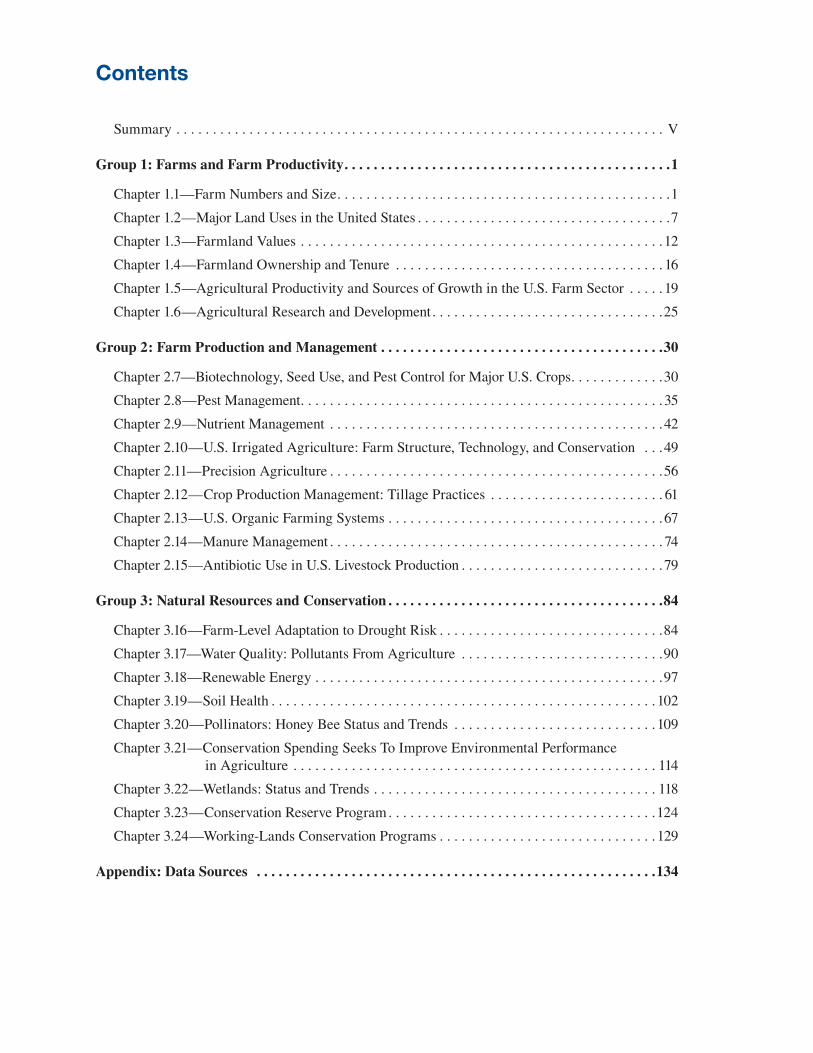
Summary . . . . . . . . . . . . . . . . . . . . . . . . . . . . . . . . . . . . . . . . . . . . . . . . . . . . . . . . . . . . . . . . . . . V
Group 1: Farms and Farm Productivity . . . . . . . . . . . . . . . . . . . . . . . . . . . . . . . . . . . . . . . . . . . . .1
Chapter 1.1—Farm Numbers and Size . . . . . . . . . . . . . . . . . . . . . . . . . . . . . . . . . . . . . . . . . . . . . .1
Chapter 1.2—Major Land Uses in the United States . . . . . . . . . . . . . . . . . . . . . . . . . . . . . . . . . . .7
Chapter 1.3—Farmland Values . . . . . . . . . . . . . . . . . . . . . . . . . . . . . . . . . . . . . . . . . . . . . . . . . .12
Chapter 1.4—Farmland Ownership and Tenure . . . . . . . . . . . . . . . . . . . . . . . . . . . . . . . . . . . . . 16
Chapter 1.5—Agricultural Productivity and Sources of Growth in the U.S. Farm Sector . . . . . 19
Chapter 1.6—Agricultural Research and Development . . . . . . . . . . . . . . . . . . . . . . . . . . . . . . . .25
Group 2: Farm Production and Management . . . . . . . . . . . . . . . . . . . . . . . . . . . . . . . . . . . . . . .30
Chapter 2.7—Biotechnology, Seed Use, and Pest Control for Major U.S. Crops . . . . . . . . . . . . .30
Chapter 2.8—Pest Management . . . . . . . . . . . . . . . . . . . . . . . . . . . . . . . . . . . . . . . . . . . . . . . . . .35
Chapter 2.9—Nutrient Management . . . . . . . . . . . . . . . . . . . . . . . . . . . . . . . . . . . . . . . . . . . . . .42
Chapter 2.10—U.S. Irrigated Agriculture: Farm Structure, Technology, and Conservation . . .49
Chapter 2.11—Precision Agriculture . . . . . . . . . . . . . . . . . . . . . . . . . . . . . . . . . . . . . . . . . . . . . .56
Chapter 2.12—Crop Production Management: Tillage Practices . . . . . . . . . . . . . . . . . . . . . . . . 61
Chapter 2.13—U.S. Organic Farming Systems . . . . . . . . . . . . . . . . . . . . . . . . . . . . . . . . . . . . . .67
Chapter 2.14—Manure Management . . . . . . . . . . . . . . . . . . . . . . . . . . . . . . . . . . . . . . . . . . . . . . 74
Chapter 2.15—Antibiotic Use in U.S. Livestock Production . . . . . . . . . . . . . . . . . . . . . . . . . . . .79
Group 3: Natural Resources and Conservation . . . . . . . . . . . . . . . . . . . . . . . . . . . . . . . . . . . . . .84
Chapter 3.16—Farm-Level Adaptation to Drought Risk . . . . . . . . . . . . . . . . . . . . . . . . . . . . . . .84
Chapter 3.17—Water Quality: Pollutants From Agriculture . . . . . . . . . . . . . . . . . . . . . . . . . . . .90
Chapter 3.18—Renewable Energy . . . . . . . . . . . . . . . . . . . . . . . . . . . . . . . . . . . . . . . . . . . . . . . .97
Chapter 3.19—Soil Health . . . . . . . . . . . . . . . . . . . . . . . . . . . . . . . . . . . . . . . . . . . . . . . . . . . . . 102
Chapter 3.20—Pollinators: Honey Bee Status and Trends . . . . . . . . . . . . . . . . . . . . . . . . . . . .109
Chapter 3.21—Conservation Spending Seeks To Improve Environmental Performance in Agriculture . . . . . . . . . . . . . . . . . . . . . . . . . . . . . . . . . . . . . . . . . . . . . . . . . . 114
Chapter 3.22—Wetlands: Status and Trends . . . . . . . . . . . . . . . . . . . . . . . . . . . . . . . . . . . . . . . 118
Chapter 3.23—Conservation Reserve Program . . . . . . . . . . . . . . . . . . . . . . . . . . . . . . . . . . . . .124
Chapter 3.24—Working-Lands Conservation Programs . . . . . . . . . . . . . . . . . . . . . . . . . . . . . . 129
Appendix: Data Sources . . . . . . . . . . . . . . . . . . . . . . . . . . . . . . . . . . . . . . . . . . . . . . . . . . . . . . .134
Contents
Agricultural Resources and Environmental
ERS is a primary source of economic research and
analysis from the U.S. Department of Agriculture,
providing timely information on economic and policy
issues related to agriculture, food, the environment, and
rural America.
United States Department of Agriculture
www.ers.usda.gov
A report summary from the Economic Research Service May 2019
United States Department of Agriculture
Economic ResearchService
Economic Information Bulletin Number 208
May 2019
Agricultural Resources and Environmental Indicators, 2019
Dan Hellerstein, Dennis Vilorio, and Marc Ribaudo (editors)
Agricultural Resources and Environmental
• As of 2017, small farms (family farms with less than $350,000 in revenue) madeup 89 percent of U.S. farms. But the 3 percent of farms with at least $1,000,000 inrevenue accounted for 39 percent of production.
• In 2012, almost 53 percent of the 2.3 billion acres of land in the United States wasused for agricultural purposes, including cropping, grazing (in pasture, range, andforests), farmsteads, and farm roads.
• Between the early 2000s and 2015, average U.S. farm real estate value nearlydoubled in inflation-adjusted terms. Since 2015, the value of cropland has de-clined by nearly 5 percent.
• In 2014, 61 percent of land in farms was owner-operated, with the remaining landrented out by the landowner to a tenant farm operator. Non-operator landlordsown 80 percent of all rented farmland.
• From 1948 to 2015, agricultural output grew 1.48 percent per year while aggre-gate input use increased only 0.1 percent annually on average.
• Since the early 2000s, private-sector food and agricultural research and develop-ment (R&D) has grown much more rapidly than public-sector R&D, so by 2014the private sector spent nearly three times as much as the public sector.
• Corn, cotton, and soybean growers have widely adopted genetically engineered(GE) herbicide-tolerant (HT) and insect-resistant (Bt) seeds since 1996. By 2018,90 percent of corn, cotton, and soybean acres planted in the United States used HTseeds, and 80 percent of corn and cotton acres used seeds also containing Bt traits.
Indicators, 2019Indicators, 2019
Daniel Hellerstein, Dennis Vilorio, and Marc Ribaudo (editors)
What Is the Issue?
Agricultural production affects a wide range of natural resources, including land, water, and air. This report provides concise information about how natural resources (land and water) and commercial inputs (energy, nutrients, pesticides, antibiotics, and other technologies) are used in the agricultural sector and how they contribute to environmental quality. To assist public and private decision making around how best to manage these resources and their impacts, the report further explores the complex links among public policies, economic conditions, farming and conservation practices, productivity and technological change, resource use, and the environment. The objec-tive is to provide a comprehensive source of data and analysis on the factors that affect resource use and quality in American agriculture.
What Did the Study Find?
Notable findings for Farms and Farm Productivity include:
Summary

www.ers.usda.gov www.ers.usda.gov
• Herbicide application rates per planted acre in 2014 compared to 2010 were up 21 percent for corn, 25 percent for cotton, 26 percent for wheat, and 24 percent for soybeans. The types of herbicides used have changed over time.
• Commercial fertilizer consumption was about 22 million short tons in 2015. For corn, winter wheat, and cotton, nitrogen recovery rates hovered around 70 percent, while phosphate recovery rates were at 60 percent.
• In 2012, irrigated farms represented about 14 percent of all U.S. farms but accounted for 39 percent of U.S. farm sales. Between 1984 and 2013, acreage in water-efficient sprinkler and drip/trickle systems rose from 37 to 76 percent of irrigated area in the Western United States.
• Precision agriculture comprises technologies such as guidance systems and variable-rate technology (VRT). By 2013, over 20 percent of planted corn, soybeans, and rice acreage were farmed using VRT.
• By the end of 2017, 44 percent of U.S. broiler chickens were raised without any antibiotics. Between 2004 and 2015, the share of finishing hogs from operations reporting that they did not know or did not report whether antibiotics were used for growth promotion rose from 7 percent to 35 percent.
• Conservation tillage, which can reduce soil erosion and sediment loss, is used on around 70 percent of soy-bean acres, 40 percent of cotton, 65 percent of corn, and 67 percent of wheat.
• U.S. organic retail sales reached an estimated $49 billion in 2017. The number of certified organic operations in the United States more than doubled between 2006 and 2016.
• Animal manure provides a source of nutrients for crops. In 2011, around 66 percent of broiler operations had a nutrient management plan, compared to 54 percent of hog operations and 41 percent of dairies.
• As of 2017, across the Nation, 55 percent of assessed rivers and streams; 71 percent of lakes; and 84 percent of bays and estuaries nationally have impaired water quality. Agriculture is the largest source of impairments in rivers and streams and the second-largest source in lakes and ponds.
• Drought is the leading cause of production risk and crop insurance indemnity payments in the United States. Practices such as irrigation adoption can reduce drought vulnerability.
• Many farmers and ranchers use practices that enhance soil health. In 2012, 35 percent of all cropland acres were in no-till and 3 percent were planted with a cover crop, two practices that promote soil health.
• Based on a land use-based measure of quality, pollinator forage habitat increased between 1982 and 2002, then declined until 2012. The decline was greatest in the Northern Plains, a summering ground for commer-cial beehives.
• Between 2007 and 2012, the number of farms producing energy or electricity onfarm with solar panels, geo-thermal exchange, wind turbines, small hydro, or methane digesters increased from 1.1 to 2.7 percent.
• Federal funding for the five largest voluntary programs that encourage land retirement and adoption of conser-vation practices on working lands was roughly $6 billion in 2017. In real (inflation-adjusted) terms, conserva-tion spending increased in the 2002 and 2008 Farm Acts and declined in the 2014 Farm Act.
• Since 1992, freshwater wetlands in the contiguous United States have held steady at around 111 million acres.
• Between 2012 and 2018, acreage enrolled in USDA’s Conservation Reserve Program (CRP) declined from 29.5 million to 22.4 million acres. However, land enrolled in the continuous portion of the CRP increased from 5.3 million to 8.1 million acres.
• In 2016, an estimated 1.7 percent of farms were enrolled in the USDA’s Environmental Quality Incentives Program (EQIP), and 5.1 percent were enrolled in the Conservation Stewardship Program (CSP).
How Was the Study Conducted?
Each chapter reflects the most recent data and information available on that topic as of July 2018. As described in the data appendix, the report relies heavily, but not exclusively, on the Agricultural Resource Management Survey (ARMS), the Census of Agriculture, and USDA Administrative data. This report was prepared before the release of the 2017 Census of Agriculture. Instead, the report uses the 2012 Census of Agriculture.
Group 1: Farms and Farm Productivity
Agricultural Resources and Environmental Indicators, 2019, EIB-208
USDA, Economic Research Service
1
Chapter 1.1—Farm Numbers and Size
Robert A. Hoppe and Christopher B. Burns
•Farmnumbersappeartohavestabilizedsincethe1970s,aftersharpdeclinesfrom1938throughtheearly 1970s.
•Asof2017,smallfarms(familyfarmswithlessthan$350,000inrevenue)madeup89percentofU.S. farms. But the 3 percent of farms with at least $1,000,000 in revenue accounted for 39 percent of production.
•Farmprogramsgenerallytargetproduction,directlyorindirectly.However,mostofthepaymentsforUSDA’s Conservation Reserve Program, which removes environmentally sensitive land from crop production, go to low-sales operations, such as retirement farms.
Farm Numbers Stabilize
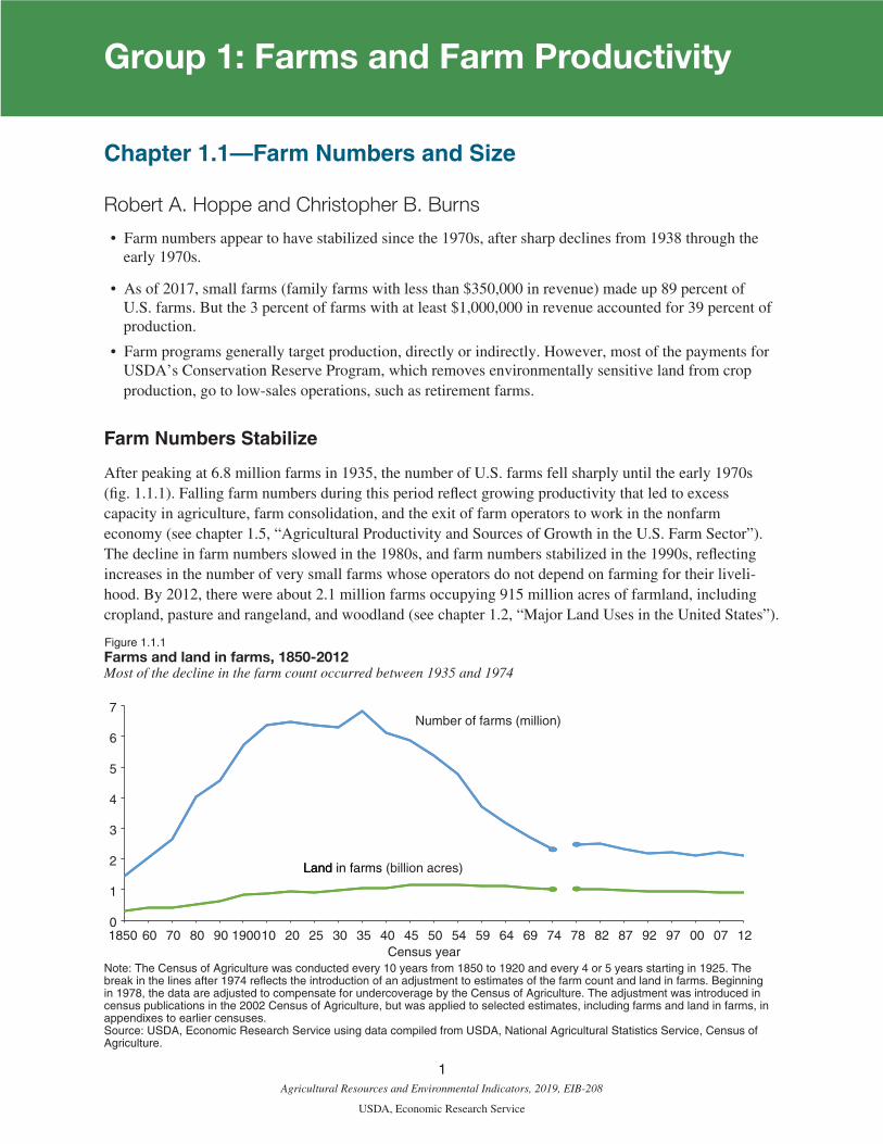
After peaking at 6.8 million farms in 1935, the number of U.S. farms fell sharply until the early 1970s (fig. 1.1.1). Falling farm numbers during this period reflect growing productivity that led to excess capacity in agriculture, farm consolidation, and the exit of farm operators to work in the nonfarm economy (see chapter 1.5, “Agricultural Productivity and Sources of Growth in the U.S. Farm Sector”). The decline in farm numbers slowed in the 1980s, and farm numbers stabilized in the 1990s, reflecting increases in the number of very small farms whose operators do not depend on farming for their liveli-hood. By 2012, there were about 2.1 million farms occupying 915 million acres of farmland, including cropland, pasture and rangeland, and woodland (see chapter 1.2, “Major Land Uses in the United States”).
Figure 1.1.1Farms and land in farms, 1850-2012Most of the decline in the farm count occurred between 1935 and 1974
0
1
2
3
4
5
6
7
1850 60 70 80 90 190010 20 25 30 35 40 45 50 54 59 64 69 74 78 82 87 92 97 00 07 12Census year
Number of farms (million)
LandLand in farms (billion acres)
Note: The Census of Agriculture was conducted every 10 years from 1850 to 1920 and every 4 or 5 years starting in 1925. The break in the lines after 1974 reflects the introduction of an adjustment to estimates of the farm count and land in farms. Beginning in 1978, the data are adjusted to compensate for undercoverage by the Census of Agriculture. The adjustment was introduced in census publications in the 2002 Census of Agriculture, but was applied to selected estimates, including farms and land in farms, in appendixes to earlier censuses. Source: USDA, Economic Research Service using data compiled from USDA, National Agricultural Statistics Service, Census of Agriculture.
Group 1: Farms and Farm Productivity

Agricultural Resources and Environmental Indicators, 2019, EIB-208
USDA, Economic Research Service
2
Some of the increase in the number of very small farms that stabilized the farm count, however, occurred because of changes in how USDA’s National Agricultural Statistics Service (NASS) conducts the Census of Agriculture. NASS now adjusts the farm count to account for undercoverage of small farms and has increased its efforts to contact all small farms for the Census. In addition, the $1,000 farm sales cutoff to qualify as a farm is not adjusted for inflation and has not changed since the current farm definition was adopted in 1974. This means that when commodity prices increase, the number of farms increases because less physical production is required to qualify as a farm. In other words, we do not know how much of the increase in small farms is due to measurement issues and how much is due to the actual entry of small farms.
While farm numbers appear to have stabilized, production has shifted to larger farms. Between 1991 and 2017, farms with gross revenue of $1 million or more (in 2017 dollars) increased their share of U.S. produc-tion from 30 percent to 39 percent. Today’s farms are diverse, ranging from very small retirement and resi-dential farms to large operations with gross revenue in the millions of dollars. It is important to differentiate between small farms that dominate the farm count and larger farms that dominate production totals.
Farm Diversity—Classifying Small and Large Farms
One way to view the diversity of farms is to categorize them into more homogeneous groups. A farm clas-sification developed by USDA’s Economic Research Service focuses on family farms, where the majority of the business is owned by the principal operator—the person most responsible for running the farm—and relatives of the principal farm operator. The classification identifies four types of small family farms (annual revenue less than $350,000): retirement, off-farm occupation, farming-occupation/low-sales, and farming-occupation/moderate-sales (see box, “Farm Types”).
Small farms dominate the farm count, making up 89 percent of all U.S. farms in 2017 (table 1.1.1). Production, however, is concentrated among the remaining groups: midsize, large, and very large family farms, as well as nonfamily farms. Together, these classes accounted for 74 percent of the value of agri-cultural production in 2017. Large-scale family farms (annual gross revenue above $1 million) alone accounted for 39 percent of U.S. farm production, while comprising only 3 percent of farms. Large-scale farms account for much larger shares of agricultural production than their share of farmland. This is largely due to their commodity mix: large-scale farms include many fruit and vegetable operations, cattle feedlots, and dairy farms, which generate high values of production on limited land bases.

Agricultural Resources and Environmental Indicators, 2019, EIB-208
USDA, Economic Research Service
3
Farm Types
The farm classification developed by the Economic Research Service (ERS) focuses on the “family farm,” or any farm where the majority of the business is owned by the principal operator—the person most responsible for operating the farm—and individuals related to the principal operator, including relatives who do not live in the operator’s household. Farm size in the classification is measured by the farm’s gross revenue, the sum of crop and livestock sales, Government pay-ments, and other farm-related income, including fees from production contracts. The USDA defines a farm as any place that produced and sold—or normally would have produced and sold—at least $1,000 of agricultural products during a given year.
Small family farms (Gross revenue less than $350,000)
Midsize family farms
Retirement farms. Small farms whose principal operators report they are retired, although they continue to farm on a small scale.
Off-farm occupation farms. Small farms whose principal operators report a primary occupation other than farming.
Farming-occupation farms. Small family farms whose principal operators report farm-ing as their primary occupation.
• Low sales. Gross revenue less than
$150,000.
• Moderate sales. Gross revenue between
$150,000 and $349,999.
Midsize family farms. Farms with gross revenue between $350,000 and $999,999.
Large-scale family farms (Gross revenue of $1,000,000 or more)
Large farms. Farms with gross revenue between $1,000,000 and $4,999,999.
Very large farms. Farms with gross revenue of $5,000,000
Nonfamily farms
Nonfamily farms. Any farm where the opera-tor and persons related to the operator do not own a majority of the business.

Agricultural Resources and Environmental Indicators, 2019, EIB-208
USDA, Economic Research Service
4
Table 1.1.1
Distribution of farms, production, farmland, and Government payments by type of farm, 2017
Type of farm Farms Value of production
Acres of farmland operated1
Commod-ity-related programs2
Conser-vation
Reserve Program3
Working land
programs4
Total payments5
Small family farms
Retirement 10.7 1.3 3.9 1.7 21.6 1.5 5.3
Off-farm occupation 40.8 4.9 17.1 5.9 28.6 10.5 10.9
Farming-occupation
Low-sales 31.7 9.5 18.2 8.7 21.9 6.4 11.0
Moderate-sales 5.7 10.3 12.7 11.3 6.5 14.2 10.9
Midsize family farms 6.3 22.7 23.2 33.0 10.3 29.3 28.1
Large-scale family farms
Large farms 2.5 23.1 15.9 30.5 5.4 29.9 25.7
Very large farms 0.3 15.6 2.4 3.8 0.4 4.0 3.2
Nonfamily farms 2.2 12.4 6.5 5.2 5.2 4.2 5.0
All farms 100 100 100 100 100 100 100
Source: USDA, Economic Research Service and USDA, National Agricultural Statistics Service, 2017 Agricultural Resource Man-agement Survey.
Multiple-Operator Farms
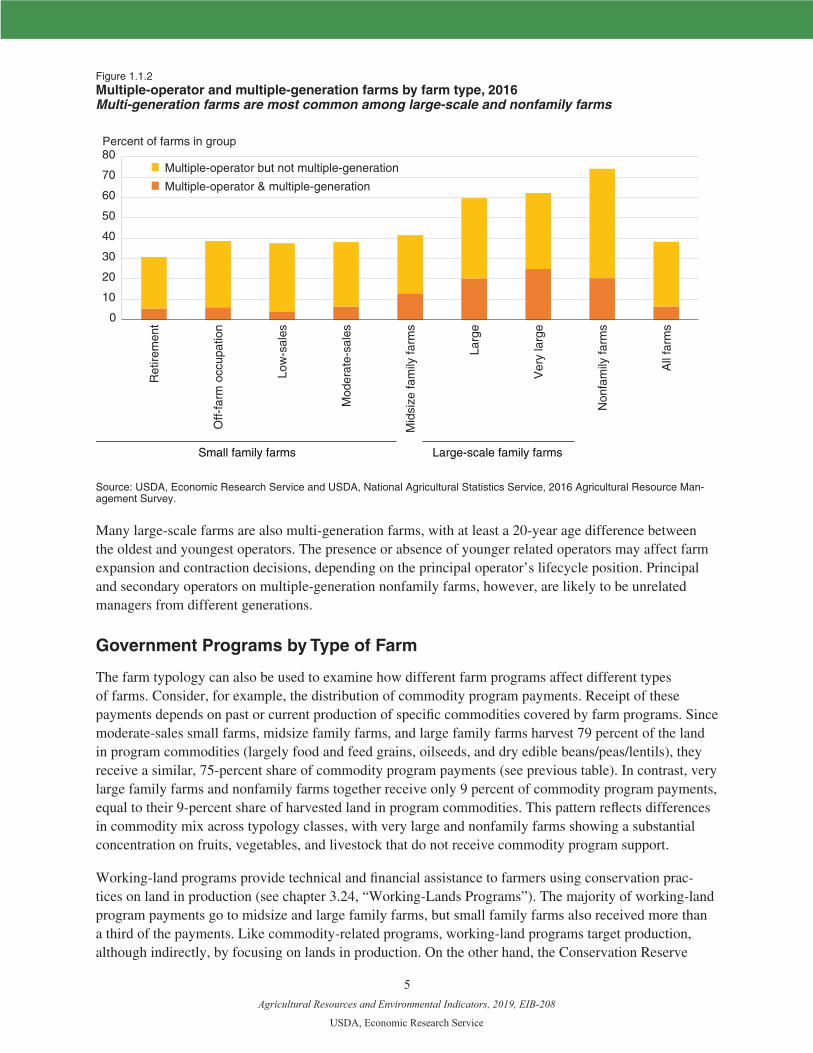
In addition to the principal operator, some farms may have additional, or secondary operators involved in running the farm business. There were 728,200 multiple-operator farms in 2016, representing 38 percent of all U.S. farms (figure 1.1.2).1 Because farms are generally family businesses, most secondary operators are family members, particularly on smaller farms. On larger farms, secondary operators are more likely to come from outside the family, and often add specific management skills needed for the farm business.
1Numbers on multiple-operator and multiple-generation farms for 2017 are not displayed due to changes in the methodology for collecting data on operator demographics in the 2017 ARMS.
Agricultural Resources and Environmental Indicators, 2019, EIB-208
USDA, Economic Research Service
5
Figure 1.1.2 Multiple-operator and multiple-generation farms by farm type, 2016 Multi-generation farms are most common among large-scale and nonfamily farms
0
10
20
30
40
50
60
70
80R
etire
men
t
Off-
farm
occ
upat
ion
Low
-sal
es
Mod
erat
e-sa
les
Mid
size
fam
ily fa
rms
Larg
e
Ver
y la
rge
Non
fam
ily fa
rms
All
farm
s
Multiple-operator & multiple-generation
Multiple-operator but not multiple-generation
Small family farms Large-scale family farms
Percent of farms in group
Source: USDA, Economic Research Service and USDA, National Agricultural Statistics Service, 2016 Agricultural Resource Man-agement Survey.
Many large-scale farms are also multi-generation farms, with at least a 20-year age difference between the oldest and youngest operators. The presence or absence of younger related operators may affect farm expansion and contraction decisions, depending on the principal operator’s lifecycle position. Principal and secondary operators on multiple-generation nonfamily farms, however, are likely to be unrelated managers from different generations.
Government Programs by Type of Farm
The farm typology can also be used to examine how different farm programs affect different types of farms. Consider, for example, the distribution of commodity program payments. Receipt of these payments depends on past or current production of specific commodities covered by farm programs. Since moderate-sales small farms, midsize family farms, and large family farms harvest 79 percent of the land in program commodities (largely food and feed grains, oilseeds, and dry edible beans/peas/lentils), they receive a similar, 75-percent share of commodity program payments (see previous table). In contrast, very large family farms and nonfamily farms together receive only 9 percent of commodity program payments, equal to their 9-percent share of harvested land in program commodities. This pattern reflects differences in commodity mix across typology classes, with very large and nonfamily farms showing a substantial concentration on fruits, vegetables, and livestock that do not receive commodity program support.
Working-land programs provide technical and financial assistance to farmers using conservation prac-tices on land in production (see chapter 3.24, “Working-Lands Programs”). The majority of working-land program payments go to midsize and large family farms, but small family farms also received more than a third of the payments. Like commodity-related programs, working-land programs target production, although indirectly, by focusing on lands in production. On the other hand, the Conservation Reserve

Agricultural Resources and Environmental Indicators, 2019, EIB-208
USDA, Economic Research Service
6
Program (CRP) targets environmentally sensitive land, not the production of commodities (see chapter 3.23, “Conservation Reserve Program: Status and Trends”). Retirement, off-farm occupation, and low-sales family farms together received 73 percent of CRP payments in 2017. Participating farmers in each of the three groups tend to enroll large shares of their land in these programs.
Because their main job is off-farm, off-farm occupation operators have limited time to spend farming. Off-farm occupation farmers may find CRP attractive because participating in the program requires little time. Given their advanced age, many retired farmers having environmentally sensitive land available may choose to participate in the CRP as they scale down their operations. The same forces may also be acting on low-sales operators, who average 62 years of age and may also be scaling down their operations.
References
Burns, Christopher B., and J.M. MacDonald. 2018. America’s Diverse Family Farms: 2018 Edition, EIB-203, U.S. Department of Agriculture, Economic Research Service, December.Hoppe, Robert A. 2014. Structure and Finances of U.S. Farms: Family Farm Report, 2014 Edition,
EIB-132, U.S. Department of Agriculture, Economic Research Service, December.Hoppe, Robert A. 2017. America’s Diverse Family Farms: 2017 Edition, EIB-185, U.S. Department of
Agriculture, Economic Research Service, December.
Agricultural Resources and Environmental Indicators, 2019, EIB-208
USDA, Economic Research Service
7
Chapter 1.2—Major Land Uses in the United States
Daniel Bigelow
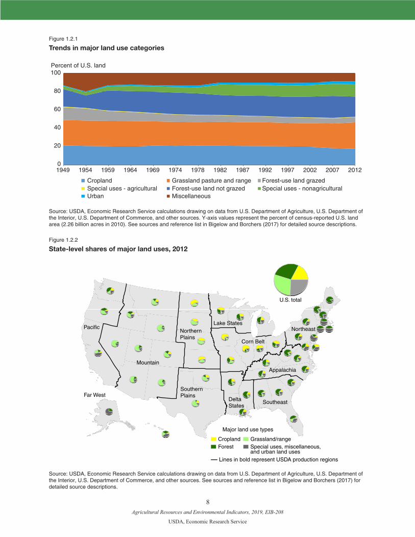
• As of 2012, grassland pasture and range (29 percent) and forest (28 percent) uses account for the largest shares of land in the United States.
• More than half of all land in the United States (53 percent) is used for some type of agricultural purpose, including crop production, grazing, farmsteads, and farm roads.
• Land use can vary substantially within regions—for example, 75 percent of Iowa is cropland versus just 41 percent of Ohio.
The U.S. land area totals nearly 2.3 billion acres. In 2012, grassland pasture and range uses accounted for the largest share of land use (29 percent of all land), followed by forest uses (28 percent) and cropland (17 percent). Just under 53 percent (1.18 billion acres) of U.S. land is used for some type of agricultural purpose, including crop production, grazing, farmsteads, and farm roads.1
Land Use Varies by Region and Over Time
Since 1949, the first year of the most recent version of the ERS Major Land Uses (MLU) data series, areas of land in the top land-use categories have fluctuated.2 For example, between 1949 and 1997, land used for grassland pasture and range decreased by 52 million acres (8 percent), but the land in this cate-gory has increased by 75 million acres (13 percent) since 1997 (figure 1.2.1). Total cropland declined by approximately 86 million acres (18 percent) between 1949 and 2012, but there were fluctuations within this interval due to Federal land retirement programs, market trends, and technological improvements. In contrast, the total acreage of urban land has exhibited a consistent upward trend over the past 60 years as cities expand to accommodate economic and population growth.
Regional land-use patterns vary based on differences in soil, climate, national and local policies and programs, topography, and population. For example, roughly 62 percent of land in the Southeast region is in forest use, compared to just 3 percent of land in the Northern Plains (figure 1.2.2). Similarly, land use varies between States within a given region. In Ohio, for instance, 41 percent of land is cropland, which contrasts with nearly 75 percent of Iowa. (State-level estimates and sources for all MLU categories are available in the ERS Major Land Uses data product.)
1In 2012, the Census of Agriculture reported that there were 914 million acres of farmland in the United States. The amount of land used for agricultural purposes reported in Major Land Uses is higher because the National Agricultural Statistics Service (USDA, NASS) definition of a farm for census purposes only covers land in operations that are capable of earning at least $1,000 in revenue in a given year and may not include all low-value land used for agricultural purposes, such as grazing.
2The Major Land Uses data series started in 1945, but did not include Alaska and Hawaii until 1949.
Agricultural Resources and Environmental Indicators, 2019, EIB-208
USDA, Economic Research Service
8
Figure 1.2.1
Trends in major land use categories
Percent of U.S. land
0
20
40
60
80
100
1949 1954 1959 1964 1969 1974 1978 1982 1987 1992 1997 2002 2007 2012
Cropland Grassland pasture and range Forest-use land grazedSpecial uses - agricultural Forest-use land not grazed Special uses - nonagriculturalUrban Miscellaneous
Source: USDA, Economic Research Service calculations drawing on data from U.S. Department of Agriculture, U.S. Department of the Interior, U.S. Department of Commerce, and other sources. Y-axis values represent the percent of census-reported U.S. land area (2.26 billion acres in 2010). See sources and reference list in Bigelow and Borchers (2017) for detailed source descriptions.
Figure 1.2.2
State-level shares of major land uses, 2012
Corn Belt
Southeast
Lake StatesNorthern Plains
Mountain
Northeast
SouthernPlains
Pacific
Far WestDeltaStates
Appalachia
U.S. total
Major land use types
CroplandForest
Grassland/rangeSpecial uses, miscellaneous, and urban land uses
Lines in bold represent USDA production regions
Source: USDA, Economic Research Service calculations drawing on data from U.S. Department of Agriculture, U.S. Department of the Interior, U.S. Department of Commerce, and other sources. See sources and reference list in Bigelow and Borchers (2017) for detailed source descriptions.
Agricultural Resources and Environmental Indicators, 2019, EIB-208
USDA, Economic Research Service
9
While land-use changes are not uncommon, most land remains in the same use from year to year. Be-tween 2007 and 2012, according to the USDA, Natural Resource Conservation Service’s (2014) National Resources Inventory, 97-99 percent of privately owned cropland (including land enrolled in USDA’s Con-servation Reserve Program (CRP)), pasture/range, urban land, and forest land did not change use. Over a longer period, 1982-2012, the rate of land-use change is larger, with 83, 86, and 91 percent of cropland/CRP land, pasture/range, and forest land, respectively, remaining in its 1982 use.
Where they occur, transitions between land uses take place for a variety of reasons. Changing commodity and timber prices, agricultural and natural resource policies, and environmental factors (such as droughts) can cause landowners to convert land from one use to another. Proximity to urban areas can also lead landowners to develop or sell their land for residential, commercial, or industrial purposes. However, in contrast to land-use changes between undeveloped uses (e.g., cropland to pasture, or vice versa), land development is generally irreversible. Once developed, land is rarely converted back to agricultural or forest-based uses.
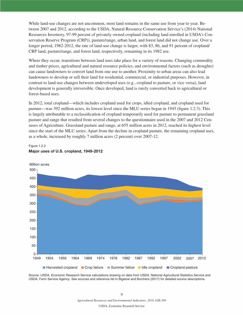
In 2012, total cropland—which includes cropland used for crops, idled cropland, and cropland used for pasture—was 392 million acres, its lowest level since the MLU series began in 1945 (figure 1.2.3). This is largely attributable to a reclassification of cropland temporarily used for pasture to permanent grassland pasture and range that resulted from several changes to the questionnaire used in the 2007 and 2012 Cen-suses of Agriculture. Grassland pasture and range, at 655 million acres in 2012, reached its highest level since the start of the MLU series. Apart from the decline in cropland pasture, the remaining cropland uses, as a whole, increased by roughly 7 million acres (2 percent) over 2007-12.
Figure 1.2.3
Major uses of U.S. cropland, 1949-2012
Million acres
0
50
100
150
200
250
300
350
400
450
500
1949 1954 1959 1964 1969 1974 1978 1982 1987 1992 1997 2002 2007 2012
Harvested cropland Crop failure Summer fallow Idle cropland Cropland pasture
Source: USDA, Economic Research Service calculations drawing on data from USDA, National Agricultural Statistics Service and USDA, Farm Service Agency. See sources and reference list in Bigelow and Borchers (2017) for detailed source descriptions.
Agricultural Resources and Environmental Indicators, 2019, EIB-208
USDA, Economic Research Service
10
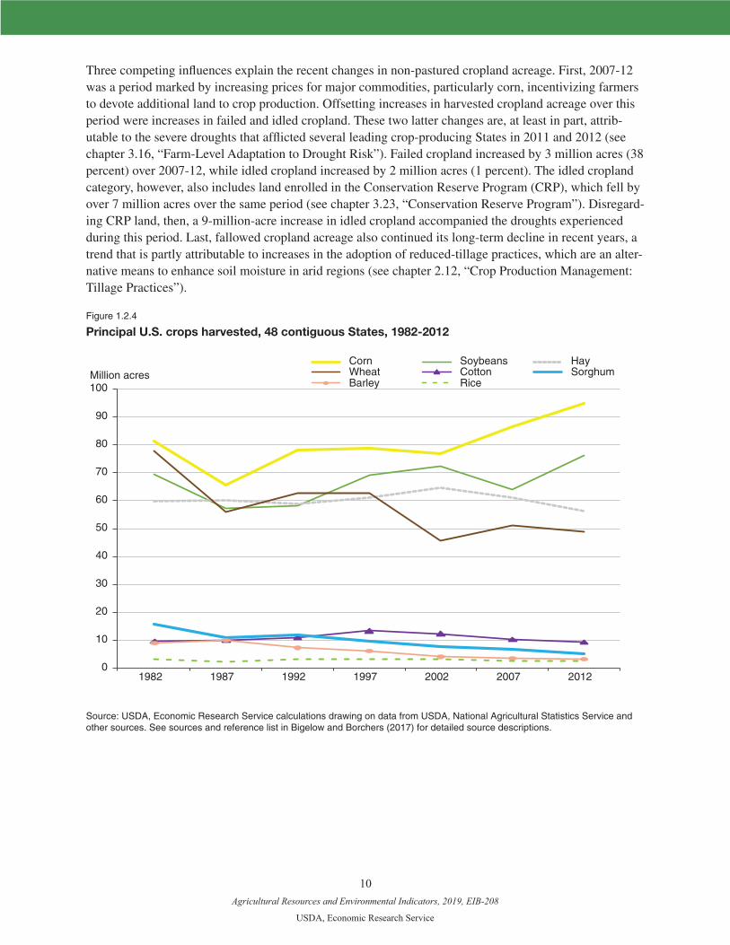
Three competing influences explain the recent changes in non-pastured cropland acreage. First, 2007-12 was a period marked by increasing prices for major commodities, particularly corn, incentivizing farmers to devote additional land to crop production. Offsetting increases in harvested cropland acreage over this period were increases in failed and idled cropland. These two latter changes are, at least in part, attrib-utable to the severe droughts that afflicted several leading crop-producing States in 2011 and 2012 (see chapter 3.16, “Farm-Level Adaptation to Drought Risk”). Failed cropland increased by 3 million acres (38 percent) over 2007-12, while idled cropland increased by 2 million acres (1 percent). The idled cropland category, however, also includes land enrolled in the Conservation Reserve Program (CRP), which fell by over 7 million acres over the same period (see chapter 3.23, “Conservation Reserve Program”). Disregard-ing CRP land, then, a 9-million-acre increase in idled cropland accompanied the droughts experienced during this period. Last, fallowed cropland acreage also continued its long-term decline in recent years, a trend that is partly attributable to increases in the adoption of reduced-tillage practices, which are an alter-native means to enhance soil moisture in arid regions (see chapter 2.12, “Crop Production Management: Tillage Practices”).
Figure 1.2.4
Principal U.S. crops harvested, 48 contiguous States, 1982-2012
Million acres
0
10
20
30
40
50
60
70
80
90
100
1982 1987 1992 1997 2002 2007 2012
Corn Soybeans Hay Wheat Cotton Sorghum Barley Rice
Source: USDA, Economic Research Service calculations drawing on data from USDA, National Agricultural Statistics Service and other sources. See sources and reference list in Bigelow and Borchers (2017) for detailed source descriptions.

Agricultural Resources and Environmental Indicators, 2019, EIB-208
USDA, Economic Research Service
11
The mix of crops grown in the United States can change in response to market incentives and agricultural policy and programs (figure 1.2.4). Increases in U.S. soybean plantings from 1995 to 2013, for instance, are contemporaneous with a large increase in exports. The decline in wheat plantings in that time period, on the other hand, occurred alongside increased foreign competition, CRP participation in wheat-pro-ducing areas, and improved corn and soybean seed varieties that allow these crops to be planted in areas previously used primarily for wheat. The use of crops as a biofuel input source has also contributed to the large gains in planted corn acreage—the main input in ethanol production—in recent decades (see, e.g., Wallander et al., 2011; Beckman et al., 2013; and chapter 3.18, “Renewable Energy”).
References
Beckman, J., A. Borchers, and C. Jones. 2013. Agriculture’s Supply and Demand for Energy and Electricity Products. U.S. Department of Agriculture, Economic Research Service, EIB-112.
Bigelow, D., and A. Borchers. 2017. Major Uses of Land in the United States, 2012. U.S. Department of Agriculture, Economic Research Service, EIB-178.
U.S. Department of Agriculture, Natural Resources Conservation Service (NRCS). 2014. Summary Report: 2012 National Resources Inventory.
Wallander, S., R. Claassen, and C. Nickerson. 2011. The Ethanol Decade: An Expansion of U.S. Corn Production, 2000-09. U.S. Department of Agriculture, Economic Research Service, EIB-79.
Agricultural Resources and Environmental Indicators, 2019, EIB-208
USDA, Economic Research Service
12
Chapter 1.3—Farmland Values
Daniel Bigelow
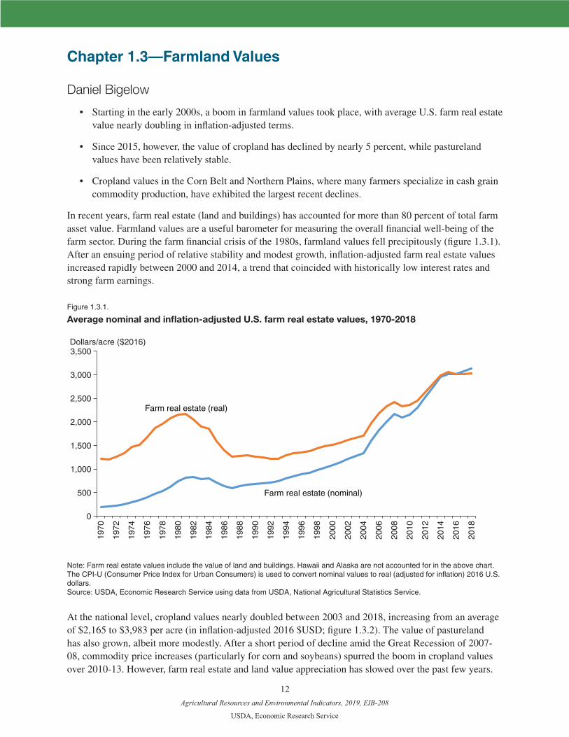
• Starting in the early 2000s, a boom in farmland values took place, with average U.S. farm real estate value nearly doubling in inflation-adjusted terms.
• Since 2015, however, the value of cropland has declined by nearly 5 percent, while pastureland values have been relatively stable.
• Cropland values in the Corn Belt and Northern Plains, where many farmers specialize in cash grain commodity production, have exhibited the largest recent declines.
In recent years, farm real estate (land and buildings) has accounted for more than 80 percent of total farm asset value. Farmland values are a useful barometer for measuring the overall financial well-being of the farm sector. During the farm financial crisis of the 1980s, farmland values fell precipitously (figure 1.3.1). After an ensuing period of relative stability and modest growth, inflation-adjusted farm real estate values increased rapidly between 2000 and 2014, a trend that coincided with historically low interest rates and strong farm earnings.
Figure 1.3.1.
Average nominal and inflation-adjusted U.S. farm real estate values, 1970-2018
Dollars/acre ($2016)
0
500
1,000
1,500
2,000
2,500
3,000
3,500
1970
1972
1974
1976
1978
1980
1982
1984
1986
1988
1990
1992
1994
1996
1998
2000
2002
2004
2006
2008
2010
2012
2014
2016
2018
Farm real estate (real)
Farm real estate (nominal)
Note: Farm real estate values include the value of land and buildings. Hawaii and Alaska are not accounted for in the above chart. The CPI-U (Consumer Price Index for Urban Consumers) is used to convert nominal values to real (adjusted for inflation) 2016 U.S. dollars.Source: USDA, Economic Research Service using data from USDA, National Agricultural Statistics Service.
At the national level, cropland values nearly doubled between 2003 and 2018, increasing from an average of $2,165 to $3,983 per acre (in inflation-adjusted 2016 $USD; figure 1.3.2). The value of pastureland has also grown, albeit more modestly. After a short period of decline amid the Great Recession of 2007-08, commodity price increases (particularly for corn and soybeans) spurred the boom in cropland values over 2010-13. However, farm real estate and land value appreciation has slowed over the past few years.

Agricultural Resources and Environmental Indicators, 2019, EIB-208
USDA, Economic Research Service
13
Between 2015 and 2018, the real value of cropland declined by nearly 5 percent. Pastureland values have been more stable, declining by less than 1 percent between 2015 and 2018.
Figure 1.3.2.
Average inflation-adjusted U.S. farmland values, 2003-2018
Dollars/acre ($2016)
0
500
1,000
1,500
2,000
2,500
3,000
3,500
4,000
4,500
2003 2004 2005 2006 2007 2008 2009 2010 2011 2012 2013 2014 2015 2016 2017 2018
Cropland
Pastureland
Note: Cropland and pastureland values reflect the value of land only. The chart excludes farmland values for Hawaii and Alaska. The CPI-U Consumer Price Index is used to convert nominal values to real (adjusted for inflation) 2016 U.S. dollars. Inflation adjust-ments for 2018 are based on the first 6 months of available 2018 data. Source: USDA, Economic Research Service using data from the USDA, National Agricultural Statistics Service (NASS), Land Values 2018 Summary. Data for years prior to 2018 are derived from earlier versions of the NASS Land Values report.
Growth in farmland values is contemporaneous with a shift in the expected stream of net returns that own-ing farmland may yield. This is influenced by factors that affect the economy as a whole, as well as those that are specific to the farm sector. For example, rising farm loan interest rates can put downward pressure on land values because the expected net returns from owning land decline when borrowing costs increase and investment alternatives become more attractive (e.g., Oppedahl, 2017). Expectations of the income stream may also be changing due to decreased commodity prices: at the end of 2017, the ratio of prices received by farmers to production costs was 13 percent lower than in 2013. In addition, 2018 USDA pro-jections indicate that the inflation-adjusted prices of three major crops will either hold constant (wheat) or exhibit modest declines (corn and soybeans) over the next 10 years (USDA, 2018).
Farmland values exhibit considerable regional variation (table 1.3.1). For example, the highest farmland values are generally found in the Corn Belt, Pacific, and Northeast regions. Land values in the Corn Belt are associated with cash-grain commodity prices and growing conditions. Hence, as a result of the 2010-13 commodity price boom, cropland values grew more rapidly in the Corn Belt than in any other region. However, since 2015, the value of cropland in the region has declined as corn and soybean prices have trended back toward their historical average. A similar downward trend in cropland value has taken place in the Northern Plains, another region where values are strongly associated with cash-grain commodity prices and production.

Agricultural Resources and Environmental Indicators, 2019, EIB-208
USDA, Economic Research Service
14
Table 1.3.1.
Regional farmland values and farmland value trends
RegionCropland, 2018
value and 2014-18 real percent change
Pastureland, 2018 value and 2014-18 real
percent change
Farm real estate, 2018 value and 2014-18 real
percent change
Appalachia 3,920 -1 3,350 -3 3,820 -1
Corn Belt 6,710 -9 2,470 0 6,430 -4
Delta States 2,820 7 2,550 7 2,980 7
Lake States 4,800 -2 2,110 3 4,890 0
Mountain 1,810 2 634 -1 1,140 1
Northeast 5,480 -1 3,480 -4 5,100 -2
Northern Plains 2,830 -13 1,070 7 2,170 -9
Pacific 6,780 10 1,650 -2 5,550 17
Southeast 3,990 2 3,990 0 3,870 1
Southern Plains 2,020 18 1,710 6 2,220 18
Note: Farm real estate is the value of both land and buildings across all types of farmland. The chart excludes farmland values for Hawaii and Alaska. The percentage changes are based on using the CPI-U Consumer Price Index to convert nominal values to real (adjusted for inflation) 2016 U.S. dollars. Inflation adjustments for 2018 are based on the first 6 months of available 2018 data.Source: USDA, Economic Research Service using data from USDA, National Agricultural Statistics Service (NASS), Land Values 2018 Summary. Data for years prior to 2018 are derived from earlier versions of the NASS Land Values report.
In contrast, the relatively high farmland values in the Northeast are mainly due to non-agricultural in-fluences (such as the expansion of urban and suburban land use) that bid up the value of farmland. As a result, cropland values in the Northeast, on average, did not show an uptick stemming from the increase in commodity prices, as they did in cash-grain production areas such as the Corn Belt. The relative depen-dence of land values on net returns to crop production is captured by patterns in cropland cash rents. For instance, cropland cash rents in the Corn Belt ($204/acre in 2018) are far higher than those in the North-east ($80.50/acre).
In many regions, the difference in value between cropland and pastureland is stark, with cropland com-manding a premium due to the higher per-acre returns associated with crop production and the relative scarcity of high-quality cropland. However, in some areas, particularly the Southeast, land values for these two uses are more comparable, with pastureland values often exceeding the value of cropland. As in the Northeast, the value of pasture in the Southeast is influenced by development pressures from high-densi-ty urban areas. Recreational income (e.g., hunting and wildlife viewing) may also play a role in pushing pastureland value above its agricultural production value (Doye and Brorsen, 2011).

Agricultural Resources and Environmental Indicators, 2019, EIB-208
USDA, Economic Research Service
15
References
Doye, D., and B. Brorsen. 2011. “Pasture land values: A ‘Green Acres’ effect?” Choices 26 (2).Oppedahl, D. 2017. AgLetter: May 2017, Federal Reserve Bank of Chicago, No. 1976, May 2017.U.S. Department of Agriculture (USDA), National Agricultural Statistics Service (NASS). 2018. Land
Values 2018 Summary. August.U.S. Department of Agriculture (USDA). 2018. USDA Agricultural Projections to 2027. Office of the
Chief Economist, World Agricultural Outlook Board. Prepared by the Interagency Agricultural Projec-tions Committee. Long-term Projections Report OCE-2018-1, 117 pp.

Agricultural Resources and Environmental Indicators, 2019, EIB-208
USDA, Economic Research Service
16
Chapter 1.4—Farmland Ownership and Tenure
Daniel Bigelow
• In 2014, 61 percent (557 million acres) of U.S. farmland was owned and operated by the same enti-ty. The remaining 39 percent of land was rented out by landowners to tenant operators. Roughly 80 percent of rented land is owned by a non-operator landlord.
• About 54 percent of all cropland was rented out, compared to just 28 percent of pastureland.
• Non-operator landlords, who own 31 percent of all U.S. farmland, own a disproportionate share (52 percent) of land where oil and gas rights have been leased.
Farmland ownership and tenure shape many decisions in the U.S. agricultural sector, including those related to production, conservation, and succession planning. In 2014, 61 percent of the 911 million acres of land in farms in the contiguous United States was owner-operated, meaning that it was owned and operated by the same farming entity (figure 1.4.1). The remaining 39 percent of land was rented out by the landowner to a tenant farm operator.
Figure 1.4.1.
U.S. farmland ownership, 2014
557 millionacres61%
70 million acres8%
138 million acres15%
53 million acres6%
32 million acres3%
51 million acres, 6%
10 million acres, 1%
284 millionacres31%
Owner-operatedRented out by operatorsRented out by non-operators
individualspartnershipscorporationstrustsother ownership arrangements
Rented out by:
Source: USDA, Economic Research Service and National Agricultural Statistics Service, 2014 Tenure, Ownership, and Transition of Agricultural Land survey.
About one-fifth of rented land (8 percent of all farmland) was rented from one farm operator to another. The remainder, about 31 percent of all farmland, was owned and rented out by “non-operator land-lords,” landowners who are not actively involved in a farm operation but own farmland and rent it out to one or more farm operators. Nearly half of the land rented out by non-operator landlords is owned by individuals, while the remainder is split between partnerships, corporations, trusts, and other ownership arrangements. In terms of land use, 54 percent of all cropland was rented out in 2014, compared to just 28 percent of pastureland. Small family farms—those with less than $350,000 in gross cash farm

Agricultural Resources and Environmental Indicators, 2019, EIB-208
USDA, Economic Research Service
17
income—are generally less reliant on rental markets, with only 31 percent of land in such operations obtained through renting.
Land tenure arrangements may affect environmental stewardship and adoption of conservation practices, since tenant farmers might lack the incentives to manage land in a way that maximizes long-term land productivity. One way to study this issue is to look at the division of decision making between landlords and tenants for different types of farm decisions. In general, tenants are responsible for day-to-day deci-sions on the vast majority of land for many aspects of farm management and production, including crop/livestock choices, fertilizer and chemical applications, and harvesting. However, landlords tend to have significantly more involvement in decisions concerning one-season conservation practices and govern-ment program participation.1
In addition, relative to operator landlords, non-operator landlords are more likely to cede control of decision-making to their tenants for many farm decisions. For example, on land rented from nonoperator landlords, tenants had sole responsibility for fertilizer and chemical application decisions on 93 percent of land, a share that drops to 83 percent for land rented from other operators (table 1.4.1). The disparity is even starker for decisions regarding one-season conservation practice adoption, where landlords are not involved in decisions on 82 percent of non-operator land versus just 67 percent of land rented out by farm operators. This suggests that operator landlords, who may have direct experience with the benefits of conservation practices, are more likely to be engaged with how these practices are adopted on the land they own regardless of whether or not they are currently operating the land.
Table 1.4.1.
Tenant responsibility for decisions by landlord type and production/management practice, 2014
Non-operator landlords (percent)
Operator landlords (percent)
Fertilizer and chemicals 93 83
Cultivation practices 91 83
Crop/livestock choices 93 86
Harvesting 95 89
Marketing 87 84
Crop insurance 83 83
One-season conservation practices 82 67
Government program participation 70 58
Note: The percentages in the table represent the percentage of total rented acres for the landlords who responded to the deci-sion section of the 2014 TOTAL questionnaire. Values in the table represent the percentages of rented acres characterized by situations where decisionmaking was solely the responsibility of the tenant. “One-season conservation practices” include reduced tillage, no till, cover cropping, and other practices that may vary from season to season. Government programs accounted for in the “Government program participation” category include both commodity and conservation programs. It is not possible to determine if the respondents actually adopted conservation practices or enrolled in Government programs. Source: USDA, Economic Research Service and National Agricultural Statistics Service 2014 Tenure, Ownership, and Transition of Agricultural Land (TOTAL) survey.
1A similar question was asked in the TOTAL survey regarding “permanent” conservation practices, such as the construction of grassed waterways and terraces. The pattern of results from this question are similar to those for one-season conservation practices.

Agricultural Resources and Environmental Indicators, 2019, EIB-208
USDA, Economic Research Service
18
Farmland ownership has gained additional attention in recent years as it relates to the leasing and sale of land for energy production. Non-operator landlords, who owned 31 percent of all U.S. farmland in 2014, control a larger share of land leased for oil and gas production (figure 1.4.2). Specifically, nonoperator landlords, some of whom do not live near the land they rent out, owned 36 percent of farmland on which oil and gas rights had been sold and 52 percent of farmland on which the rights had been leased. This suggests that entities that own farmland, but are not directly involved in its use for agricultural production, may be more likely to exercise nonagricultural use rights to gain access to additional streams of income.
Figure 1.4.2.
Oil and gas (O&G) production rights sales and leases by ownership type
0 10 20 30 40 50 60 70 80 90 100
Total farmland owned
Land leased for O&G production
Land sold for O&G production
Percentage of total land
Non-operator landlords Operator landowners
Source: USDA, Economic Research Service and National Agricultural Statistics Service; 2014 Tenure, Ownership, and Transition of Agricultural Land survey.
References
Bigelow, D., A. Borchers, and T. Hubbs. 2016. U.S. Farmland Ownership, Tenure, and Transfer. U.S. Department of Agriculture, Economic Research Service, EIB-161.

Agricultural Resources and Environmental Indicators, 2019, EIB-208
USDA, Economic Research Service
19
Chapter 1.5—Agricultural Productivity and Sources of Growth in the U.S. Farm Sector
Sun Ling Wang
• By 2015, U.S. farm output was about 2.7 times its 1948 level, growing at an average annual rate of 1.48 percent.
• Since aggregate input use increased only 0.1 percent annually, the positive growth in farm sector output was due almost entirely to increased productivity, which grew at an average annual rate of 1.38 percent.
• The composition of the input mix has changed markedly, shifting away from labor and land toward machinery and intermediate goods such as fertilizer and pesticides.
According to ERS’s agricultural productivity accounts (USDA, Economic Research Service, 2017), in 2015, the U.S. farm sector used about 75 percent less labor input and 25 percent less farmland than in 1948.1 Nevertheless, total agricultural production has nearly tripled over this 67-year span. The ability to produce more with much less farmland and labor is attributed mainly to the advancement in agricultural productivity, which is mostly driven by innovations in animal and crop genetics, chemicals, equipment, and farm organization.
Productivity can be measured by a single factor, like corn production per acre (yield or land productivity) or per unit of labor (labor productivity). But such measures can be misleading. For example, yields could increase through technology adoption or simply because farmers are adding more of other inputs, such as chemicals or machinery. Average national corn yield rose from around 30 bushels per acre in the 1930s to nearly 180 bushels per acre in the present decade. While this sustained growth in corn yield was driven mostly by the development and rapid adoption of successive biological, chemical, and mechanical inno-vations (fig. 1.5.1; also see chapter 2.7, “Biotechnology and Seed Use for Major U.S. Crops”), it was also due in part to heavier use of non-land inputs. Properly accounting for all input changes when measuring agricultural productivity is important to better understand the sources of growth. USDA’s Economic Research Service (ERS) develops measures of total factor productivity (TFP), which account for the use of all inputs under the control of farmers in the production of all commodities (USDA-ERS, 2017). Specifically, TFP growth is the difference between the growth of aggregate output and the growth of all inputs taken together. TFP, therefore, measures changes in the efficiency with which inputs are trans-formed into outputs.
According to ERS measures, U.S. agricultural output has grown significantly since 1948. By 2015, U.S. farm output was about 2.7 times its 1948 level, growing at an average annual rate of 1.48 percent. Aggregate input use increased only 0.1 percent annually over this time span. Therefore, the positive growth in farm-sector output was due almost entirely to growth in total factor productivity, which aver-aged 1.38 percent annually (fig. 1.5.2). Since productivity growth is a measure of output growth that cannot be explained by input growth, we discuss the patterns of output and input growth first to better understand growth of TFP and its importance to output growth.
1Farmland consists primarily of land used for crops, pasture, or grazing but also includes acres of idled cropland and wood-land. In the U.S. agricultural productivity accounts, land stock is measured as the real value of total farmland, which is nominal land value deflated by a land price index from ERS’s productivity accounts. In addition, the land stock is also adjusted by quality differences across counties and States.

Agricultural Resources and Environmental Indicators, 2019, EIB-208
USDA, Economic Research Service
20
Figure 1.5.1
Effect on corn yields as different innovations become adopted, 1920-2014
0
36
72
108
144
180
0
20
40
60
80
100
1920 1930 1940 1950 1960 1970 1980 1990 2000 2010
bushels or lbs/acrePercent of planted area
HerbicideHybrid seed Corn yield
Tractor guidancesystem
GM seed
Note: GM = genetically modified.Source: USDA, Economic Research Service analysis using data from the National Agricultural Statistics Service, Agricultural Statistics yearbook and the Agricultural Resource Management Survey.
Figure 1.5.2
TFP growth accounted for most of the U.S. agricultural output growth between 1948 and 2015
0
0.5
1.0
1.5
2.0
2.5
3.0
1948 1953 1958 1963 1968 1973 1978 1983 1988 1993 1998 2003 2008 2013
Index, 1948=1
Total outputTotal farm inputTotal factor productivity (TFP)
Source: USDA, Economic Research Service, “Agricultural Productivity in the U.S.” series.

Agricultural Resources and Environmental Indicators, 2019, EIB-208
USDA, Economic Research Service
21
Patterns in Output, Input, and Productivity Growth
Output growth derives from growth in the use of inputs (capital, land, labor, and intermediate goods) and TFP. Input growth has been the main source of economic growth for the U.S. aggregate economy and for most sectors, but the agricultural sector is different (Jorgenson et al., 2014). While total farm output grew 170 percent from 1948 to 2015, total inputs used in agriculture grew by only 7 percent. Nevertheless, the input composition changed markedly, shifting from labor and land toward machinery and intermediate goods (including energy, agricultural chemicals, purchased services, and other materials) (fig. 1.5.3). Between 1948 and 2015, labor and land inputs declined by about 75 and 25 percent, respectively, while intermediate goods and capital (excluding land) grew by 134 percent and 78 percent, respectively.
Figure 1.5.3
Inputs composition has changed over time
Index, 1948=1
0.0
0.5
1.0
1.5
2.0
2.5
3.0
1948 1958 1968 1978 1988 1998 2008
Total output
Capital (excluding land)Land
Labor
Intermediate goods
Note: Data are expressed with an index that is calculated relative to the data in 1948, where data in 1948 are set to equal 1. Intermediate goods include feed and seed, energy use, fertilizer and lime, pesticides, purchased services, and other materials used.
Source: USDA, Economic Research Service, “Agricultural Productivity in the U.S.” series.
Labor
Farm labor fell consistently from 1948 until more recent years. Productivity growth in U.S. agriculture is all the more remarkable given labor’s long-term contraction. Over 1948-2015, agricultural labor declined on average 0.46 percent each year—a rate unmatched by any other economic sector. The decline in farm labor (both farmers and hired laborers) occurred as workers sought higher wages and other income oppor-tunities in the nonfarm sector, and/or as farmers relied more on machinery use and purchased services—including custom machinery work and contract labor service (Wang et al., 2015).

Agricultural Resources and Environmental Indicators, 2019, EIB-208
USDA, Economic Research Service
22
Capital (excluding land)
Capital input (including the flow of services from farm machinery, service buildings, and inventory) in agriculture increased sharply just after WWII, reflecting rapid mechanization in U.S. agriculture. During 1973-79, U.S. agriculture expanded rapidly, fueled by a growth in exports. Agricultural exports continued to grow until 1981. Real (inflation-adjusted) interest rates also fell or remained very low between 1975 and 1980—which decreased the cost of investment. As a result, farmers invested more in farm machinery, service buildings, and inventories. However, in the early 1980s, an appreciating U.S. dollar slowed agricultural exports. Declining demand for U.S. agricultural commodity exports and rising borrowing costs reduced farmers’ incentives for further investment in farm machinery and structures. Capital investment declined between 1979 and 1986 and remained stable until the 2000s, when rising agricultural commodity prices and declining real interest rates once again spurred increased investment in machinery and service buildings (see Wang et al., 2015, for more detailed discussion.)
Land and intermediate goods
Land2 input has decreased consistently at an average rate of -0.41 percent per year. Over 1948-2015, declining land use put downward pressure on output growth, contributing -0.05 percentage points to output growth per year, on average (table 1.5.1). The positive growth in intermediate goods (fertil-izer, pesticides, fuel, etc.) largely reflects the increasing substitution of those inputs for land and labor. Intermediate goods’ contribution to output growth averaged 0.6 percent per year over 1948-2015. During 1973-79, when strong export demand fueled dramatic growth in agricultural output that outpaced TFP growth, the growth of intermediate goods contributed 1.65 percentage point per year to output growth. Overall, growing use of intermediate goods offset the negative contributions of labor and land, making the contribution of all inputs essentially flat (0.1 percent) over 1948-2015.
Total factor productivity growth
TFP growth measures output growth that cannot be explained by growth in inputs, such as innovations in onfarm tasks, changes in the organization and structure of the farm sector, improvements in animal and crop genetics, or other embodied and disembodied technical changes.3 Between 1948 and 2015, TFP grew at 1.38 percent per year on average. As a result, by 2015, U.S. farm-sector productivity was 152 percent above its 1948 level. With total inputs (including land, labor, capital, and intermediate inputs) growing by merely 7 percent, productivity growth nearly single-handedly led farm output to grow 170 percent above its 1948 level.
Long-term TFP growth is mainly driven by technical change, which is primarily fueled by research and development (R&D) investment from public and private sectors (see chapter 1.6, “Agricultural Research and Development,” for more details). It can also be enhanced by public infrastructure, extension, and technology spillover from other sectors or neighboring regions (Wang et al., 2015). Yet, in the short term, estimated TFP can fluctuate considerably from year to year, largely in response to transitory events—such as bad weather and pest outbreaks—or to changes in input use affected by macroeconomic activities or short-term policies. Eventually, TFP growth will return to its long-term trend following these temporary shocks.
2See Wang et al. (2015) and Ball et al. (2016) for more details regarding how land input is measured in U.S. agricultural productivity accounts.
3Embodied technical change (ETC) originally referred to the technological advances embodied in the capital goods that make equipment work faster or better in some way. This term can be applied to other inputs when the quality of that input is improved. Disembodied technical change is technical change not associated with any particular input.

Agricultural Resources and Environmental Indicators, 2019, EIB-208
USDA, Economic Research Service
23
Sources of Agricultural Output Growth
In addition to long-term trends, ERS also examines the sources of agricultural output growth—appor-tioning increases in output among changes in inputs (both quantities and quality/composition) and TFP—for the entire period and in 12 subperiods (defined by business cycles in accordance with fluctuations in the overall U.S. economy) (table 1.5.1).
Between 1948 and 2015, farms shifted to higher quality labor, mainly due to a more highly educated labor force. Increased labor quality made a positive contribution to output growth in 11 of 12 subperiods (table 1.5.1). On average, labor quality through changes in farm labor’s educational attainment and other demo-graphic characteristics contributed to output growth at 0.12 percentage points a year, offsetting part of the contraction in labor quantity. Still, over the entire period, the decline in overall labor input contributed negatively to output growth by nearly -0.5 percent per year. On the other hand, while the changes from durable equipment, service buildings, and inventory (capital, excluding land) made positive contributions to output growth in 9 of 12 subperiods, shrinking land use still made overall contribution of aggregate capital (including land) to output growth of -0.04 percentage points per year. Growth in intermediate goods contributed positively to output growth in 9 of 12 subperiods and accounted for about two-fifths of output growth for the entire period, offsetting negative contributions from labor and capital to output growth.
Table 1.5.1
Sources of growth in U.S. farm sector, 1948-2015 (average annual growth rates in percent)
1948-2015
1948-1953
1953-1957
1957-1960
1960-1966
1966-1969
1969-1973
1973-1979
1979-1981
1981-1990
1990-2000
2000-2007
2007-2015
Output growth 1.48 0.96 0.49 3.72 1.12 2.24 2.50 2.45 2.57 0.79 1.79 1.03 0.72
Sources of growth
Input growth 0.10 0.66 -0.03 0.75 -0.09 0.00 0.36 1.69 -1.21 -1.32 0.24 0.11 0.20
Labor -0.46 -0.83 -1.11 -0.88 -0.86 -0.65 -0.41 -0.19 -0.23 -0.45 -0.23 -0.38 0.00 Capital (including land) -0.04 0.57 -0.02 0.00 0.04 0.16 -0.10 0.23 0.11 -0.78 -0.17 -0.12 0.24
Intermediate goods 0.60 0.92 1.10 1.62 0.73 0.48 0.87 1.65 -1.09 -0.09 0.64 0.60 -0.04
TFP growth 1.38 0.30 0.52 2.97 1.20 2.24 2.14 0.75 3.79 2.11 1.55 0.92 0.53
Sources decomposition
Labor
Hours -0.57 -1.06 -1.24 -0.92 -1.14 -0.95 -0.46 -0.21 -0.20 -0.52 -0.41 -0.40 -0.08
Quality 0.12 0.23 0.12 0.04 0.28 0.30 0.05 0.01 -0.03 0.07 0.18 0.02 0.08
Capital
Capital (excluding land)
0.01 0.55 0.12 0.13 0.10 0.36 0.18 0.23 0.22 -0.69 -0.17 -0.07 0.15
Land -0.05 0.02 -0.14 -0.13 -0.06 -0.20 -0.28 0.01 -0.12 -0.09 0.00 -0.05 0.09
Intermediate goods
Quantity 0.64 1.01 0.91 1.74 0.76 0.26 0.98 1.89 -1.51 -0.02 0.61 0.63 0.15
Composition -0.04 -0.09 0.20 -0.12 -0.03 0.23 -0.11 -0.24 0.41 -0.07 0.03 -0.03 -0.19
Notes: The subperiods are measured from cyclical peak to peak in aggregate economic activity. Labor, capital, and intermediate inputs aggregate across different attributes within each input aggregate, including gender, age, educational attainment, and employment types for labor; durable equipment, service buildings, land, and inventories for capital; and feed/seed, energy, fertilizers, pesticides, purchased services and other mate-rials for intermediate goods. The contribution of an input aggregate to growth reflects changes in the quantity and quality (composition of specific components) of the aggregate.
Source: USDA, Economic Research Service, “Agricultural Productivity in the U.S.” series, updated October 2017.

Agricultural Resources and Environmental Indicators, 2019, EIB-208
USDA, Economic Research Service
24
During 1948-2015, the net contribution of all inputs was 0.1 percentage point per year, leaving TFP growth the major source of output growth in all but the 1948-1953 and 1973-79 subperiods. Since the United States is one of the largest producers and consumers in the world agricultural commodity market, sustainable productivity growth in the U.S. farm sector is critical to global food security. Given that inno-vation fueled by R&D is the major driver of productivity growth (see chapter 1.6, “Agricultural Research and Development,” for more discussion), steadily growing investment in agricultural research is essential if agricultural production is to meet growing worldwide demand.
References
Ball, Eldon, Sun Ling Wang, Richard Nehring, and Roberto Mosheim. 2016. “Productivity and Economic Growth in U.S. Agriculture: A New Look,” Applied Economic Perspectives and Policy 38(1): 30-49.
Clancy, Matthew, Keith Fuglie, and Paul Heisey. 2016. “U.S. Agricultural R&D in an Era of Falling Pub-lic Funding,” Amber Waves. November. U.S. Department of Agriculture, Economic Research Service.
Jorgenson, D.W., M.S. Ho, and J.D. Samuels. 2014. “What Will Revive U.S. Economic Growth? Lessons from a Prototype Industry-Level Production Account for the United States,” Journal of Policy Model-ing 36: 674-691
U.S. Department of Agriculture, Economic Research Service. “Agricultural Productivity in the U.S.” data product, updated October 2017.
Wang, Sun Ling, Paul Heisey, David Schimmelpfennig, and Eldon Ball. 2015. Agricultural Productivity Growth in the United States: Measurement, Trends, and Drivers. U.S. Department of Agriculture, Eco-nomic Research Service. ERR-189.
Agricultural Resources and Environmental Indicators, 2019, EIB-208
USDA, Economic Research Service
25
Chapter 1.6—Agricultural Research and Development
Paul Heisey
• Both private and public sectors help fund agricultural research and development (R&D), but due to its rapid growth, private spending is now much greater than public spending—which fell in real terms between 2006 and 2014. Private research spending on agricultural input R&D alone—not including food research—surpassed total public spending in 2010.
• In 2014, the private sector funded over three-quarters of all food and agricultural R&D in the United States.
• Public and private agricultural R&D investments are generally complementary rather than compet-itive. For example, in 2014, the private sector dominated farm machinery and food manufacturing research, while the public sector performed nearly all U.S. research on the environment/natural resources and human nutrition/food safety.
The growth in agricultural productivity over the past seven decades (see chapter 1.5, “Agricultural Produc-tivity and Sources of Growth in the U.S. Farm Sector”) can be attributed largely to investments in agricul-tural research and technology development (OECD, 2016; Wang et al., 2013). Genetic improvements in crops and livestock, improved agricultural chemicals and fertilizers, more efficient agricultural machinery, and cost reductions in farm management techniques have transformed U.S. agriculture.
As agricultural productivity has increased, the agricultural research portfolio has expanded to include areas such as the environment; the quality, safety, and nutritional value of food products; the treatment of farm animals; the livelihoods of farm workers; and the resilience of rural communities. These objectives have refocused public agricultural research to include the characteristics of agricultural products and the impacts of production methods, in addition to technology development. Corporate agribusiness has played an increasingly larger role in developing new technologies and providing services for agriculture.
Multiple Institutions Operate in a Complex System
Agriculture has benefited from a unique Federal-State partnership in agricultural research and exten-sion, with a history of collaboration with the private sector. The funders of agricultural and food research include nongovernmental sources—primarily the private business sector, but also foundations and farmer organizations—that provided over three-quarters of the funding in 2014, or about $12.4 billion in real (inflation-adjusted) dollars.1 The Federal Government—including USDA as well as other agencies such as the National Science Foundation (NSF) and the National Institutes of Health (NIH)—contributed $2.6 billion, and State governments just under $1 billion (fig. 1.6.1).
1All estimates of research spending in this chapter are adjusted for inflation to 2012 dollars using the ERS research deflator. Inconsistencies in one of the major series underlying this deflator—faculty salaries for U.S. educational institutions—preclude updating the base year to 2017.

Agricultural Resources and Environmental Indicators, 2019, EIB-208
USDA, Economic Research Service
26
Figure 1.6.1
Funders and performers of U.S. food and agricultural research in 2014 (in 2012 dollars)
Note: All estimates are adjusted for inflation and expressed in 2012 dollars using the ERS research deflator. NSF = National Science Foundation; NIH = National Institutes of Health. LGU-SAES = Land Grant Universities/State Agricultural Experiment Stations.Source: USDA, Economic Research Service based on data from the Current Research Information System; USDA, National Institute of Food and Agriculture; National Science Foundation Federal Funds for Research and Development; and Fuglie (2016).
Performers of agricultural research include Federal researchers, who generally study issues of national importance and accounted for about $1.3 billion of research spending in 2014. State-level research at the Land Grant Universities/State Agricultural Experiment Stations (LGU-SAES) and other cooperating institutions, usually other universities, accounted for $2.9 billion. Research at these academic institutions is typically directed at issues of local and regional importance and at fundamental scientific questions.
Industry was the largest performer of food and agricultural research in 2014, at $11.8 billion (fig. 1.6.1).Private-sector research is usually nearest the marketplace. Roughly half of private-sector research was spent in the food sector, where much of it is oriented toward improving food manufacturing processes and developing new food products. The other half goes toward research related to agricultural inputs, which is much more likely to have a direct impact on production agriculture.
The U.S agricultural research system is characterized by numerous links between institutions. State-level institutions receive funds from several Federal agencies other than USDA, and USDA funds State-level institutions through a variety of instruments. The private sector and USDA exchange funds or conduct joint research through grants, cooperative agreements, contracts, and trusts. USDA, State-level institutions, and private firms all transfer technology through the patent-licensing mechanism or research consortia.
Private-Sector Research Has Increased While Public Research Has Fallen
Historically, public institutions played a direct role in developing new agricultural technologies and encouraging their commercialization and adoption by farmers. Advances in the biological sciences, broader intellectual property rights protection, and expansion of agricultural markets have stimulated private-sector R&D.

Agricultural Resources and Environmental Indicators, 2019, EIB-208
USDA, Economic Research Service
27
Since about 1980, growth rates in public R&D have been generally low (fig. 1.6.2). Growth in private investment has generally been higher, but with greater variation. In the early 2000s, public and private agricultural research investments began to diverge more rapidly. Total private agricultural and food R&D doubled between 2003 and 2014, while public R&D fell. By 2010, private R&D for agricultural inputs alone surpassed the public level for all agricultural research.
Figure 1.6.2
Real agricultural research and development (R&D) funding, 1970-2015
$ billion (2012)
0
2
4
6
8
10
12
1970 1975 1980 1985 1990 1995 2000 2005 2010 2015
Public ag R&D
Total private food & ag R&D
Private R&D in agricultural inputs
Private R&D in food manufacturing
Note: Data are adjusted for inflation and expressed in 2012 dollars. Source: USDA, Economic Research Service.
Focus of Private and Public R&D Differs
In many ways public and private agricultural research efforts are complementary rather than competitive. Little incentive exists for private firms to pursue research whose results benefit society as a whole rather than the specific innovator. The incentives that encourage firms to fund and perform R&D are private returns (i.e., the economic benefits from new products and technologies that can be captured through market sales). But companies cannot capture all the potential economic benefits from R&D activities. Some benefits may accrue to farmers as lower production costs even after higher prices from new tech-nologies have been taken into account. Some R&D benefits may go to consumers in the form of safer or cheaper food. Benefits may go to other firms that develop related applications from the scientific informa-tion generated, even from other private research, as private research is only partially protected by intel-lectual property like patents or by trade secrets. Still other benefits are enjoyed by society as a whole, in the form of better health or improved environmental quality. The social returns (benefits to society as a whole) from many kinds of research can be much higher than their private return.
Thus, the private sector focuses mainly on R&D related to marketable goods and technologies. The food industry, which has little impact on agricultural productivity, accounts for the largest category of private agricultural R&D. Much food industry R&D is directed toward product development and marketing
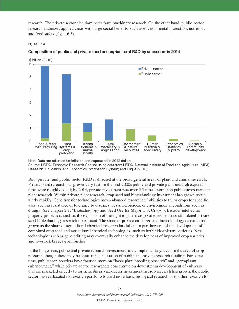
Agricultural Resources and Environmental Indicators, 2019, EIB-208
USDA, Economic Research Service
28
research. The private sector also dominates farm machinery research. On the other hand, public-sector research addresses applied areas with large social benefits, such as environmental protection, nutrition, and food safety (fig. 1.6.3).
Figure 1.6.3
Composition of public and private food and agricultural R&D by subsector in 2014
$ billion (2012)
0
1
2
3
4
5
6
Food & feedmanufacturing
Plantsystems &
cropprotection
Animalsystems &
animalhealth
Farmmachinery &engineering
Environment& naturalresources
Humannutrition &food safety
Economics,statistics& policy
Social &community
development
Private sector
Public sector
Note: Data are adjusted for inflation and expressed in 2012 dollars.Source: USDA, Economic Research Service using data from USDA, National Institute of Food and Agriculture (NIFA), Research, Education, and Economics Information System; and Fuglie (2016).
Both private- and public-sector R&D is directed at the broad general areas of plant and animal research. Private plant research has grown very fast. In the mid-2000s public and private plant research expendi-tures were roughly equal; by 2014, private investment was over 2.5 times more than public investments in plant research. Within private plant research, crop seed and biotechnology investment has grown partic-ularly rapidly. Gene transfer technologies have enhanced researchers’ abilities to tailor crops for specific uses, such as resistance or tolerance to diseases, pests, herbicides, or environmental conditions such as drought (see chapter 2.7, “Biotechnology and Seed Use for Major U.S. Crops”). Broader intellectual property protection, such as the expansion of the right to patent crop varieties, has also stimulated private seed-biotechnology research investment. The share of private crop seed and biotechnology research has grown as the share of agricultural chemical research has fallen, in part because of the development of combined crop seed and agricultural chemical technologies, such as herbicide-tolerant varieties. New technologies such as gene editing may eventually enhance the development of improved crop varieties and livestock breeds even further.
In the longer run, public and private research investments are complementary, even in the area of crop research, though there may be short-run substitution of public and private research funding. For some time, public crop breeders have focused more on “basic plant breeding research” and “germplasm enhancement,” while private-sector researchers concentrate on downstream development of cultivars that are marketed directly to farmers. As private-sector investment in crop research has grown, the public sector has reallocated its research portfolio toward more basic biological research or to other research for

Agricultural Resources and Environmental Indicators, 2019, EIB-208
USDA, Economic Research Service
29
which private firms cannot capture all the benefits through the prices they charge. Public research gener-ally operates on a longer timeframe as well, allowing it to address problems with lower probabilities of short-term payoff.
U.S. agricultural productivity growth has been marked by large increases in aggregate output with almost no change in aggregate input use (see chapter 1.5, “Agricultural Productivity and Sources of Growth in the U.S. Farm Sector”). R&D has been a major driver of agricultural productivity growth (OECD, 2016), and the research-related changes in agricultural technology that have accompanied productivity growth have therefore influenced both input use and the environmental impacts of agriculture.
References
Clancy, Matthew, Keith Fuglie, and Paul Heisey. 2016. “U.S. Agricultural R&D in an Era of Falling Public Funding,” Amber Waves. U.S. Department of Agriculture, Economic Research Service, Nov. 10.
Fuglie, Keith. 2016. “The Growing Role of the Private Sector in Agricultural Research and Development World-wide,” Global Food Security 10: 29-38.
Fuglie, Keith O., Paul W. Heisey, John L. King, Carl E. Pray, Kelly Day-Rubenstein, David Schimmel- pfennig, Sun Ling Wang, and Rupa Karmarkar-Deshmukh. 2011. Research Investments and Market Structure in the Food Processing, Agricultural Input, and Biofuel Industries Worldwide. ERR-130. U.S. Department of Agriculture, Economic Research Service, December.
Fuglie, Keith, and Paul Heisey. 2007. Economic Returns to Public Agricultural Research. EB-10. U.S. Department of Agriculture, Economic Research Service, September.
Fuglie, Keith O., and Andrew A. Toole. 2014. “The Evolving Institutional Structure of Public and Private Agricultural Research,” American Journal of Agricultural Economics 96(3): 862-883.
MacDonald, James M. 2017. “Mergers and Competition in Seed and Agricultural Chemical Markets,” Amber Waves, U.S. Department of Agriculture, Economic Research Service, April.
Organisation for Economic Co-operation and Development (OECD). 2016. Innovation, Agricultural Productivity and Sustainability in the United States. OECD Food and Agricultural Reviews. Paris: OECD Publishing.
Wang, Sun Ling, Paul W. Heisey, Wallace E. Huffman, and Keith O. Fuglie. 2013. “Public R&D, Private R&D, and U.S. Agricultural Productivity Growth: Dynamic and Long-Run Relationships,” American Journal of Agricultural Economics 95(5): 1287-1293.
Group 2: Farm Production and Management
Agricultural Resources and Environmental Indicators, 2019, EIB-208
USDA, Economic Research Service
30
Chapter 2.7—Biotechnology, Seed Use, and Pest Control for Major U.S. Crops
Seth Wechsler
• Adoption rates for genetically engineered (GE) crops rose rapidly in the years following their com-mercialization in 1996. As of June 2018, approximately 9 out of every 10 acres of domestic corn, cotton, soybeans, sugarbeets, and canola were cultivated using GE seeds; approximately 80 percent of U.S. corn and 82 percent of cotton acreage was planted with seeds that were “stacked,” or geneti-cally engineered to be both herbicide tolerant (HT) and insect resistant (Bt).
• The commercialization of Bt crops led to a decrease in synthetic soil-applied and foliar insecticide use; for example, insecticide use among U.S. corn farmers fell by over 80 percent from 1996 to 2017.
• Initially, the commercialization of HT crops led to increases in glyphosate use and decreases in the use of other herbicides. Recently, the use of glyphosate, and the use of herbicides other than gly-phosate, has increased—largely due to the development and spread of glyphosate-resistant weeds.
Adoption Rates for Genetically Engineered Crops Rose Rapidly in the Early 21st Century
Building on the results of public biomedical research, large life-science companies invested millions of dollars in efforts to develop profitable crop biotechnologies throughout the 1980s. These efforts culminat-ed in 1996 with the commercialization of genetically engineered (GE) corn, soybean, and cotton crops. GE canola was commercialized in 1998. GE alfalfa and sugarbeets were commercialized in 2005.
Herbicide-tolerant, or HT, crops are not damaged when they are sprayed with broad-spectrum herbicides (such as glyphosate or glufosinate) that damage most conventional varieties. Planting HT crops allows farmers to use nonselective, broad-spectrum herbicides throughout the growing season (even after crop emergence). Insect-resistant crops contain genes from a soil bacterium (Bacillus thuringiensis) that produc-es a naturally occurring insecticide. Unlike conventional insecticides, which can be leached from soils or adversely affected by soil pH, the toxins produced by Bt crops are concentrated in plant tissues. So, planting Bt crops helps ensure that insects are controlled throughout the growing season.
Adoption rates for GE crops rose rapidly in the decade following their commercialization. As of 2017, approximately 9 out of every 10 acres of corn, cotton, soybeans, sugarbeets, and canola produced in the United States were cultivated using HT seeds (figure 2.7.1). Approximately 8 of every 10 acres of corn and cotton acres were cultivated using Bt seeds (figure 2.7.2). Although other GE traits have been de-veloped (such as virus, fungus, cold, and drought resistances), crops with HT and Bt traits are the most prominent of the commercially available, genetically engineered varieties. Most GE corn and cotton seeds are “stacked” with both HT and Bt traits. As of 2017, approximately 80 percent of U.S. corn and cotton acreage was planted with stacked seeds (figure 2.7.3).
Group 2: Farm Production and Management

Agricultural Resources and Environmental Indicators, 2019, EIB-208
USDA, Economic Research Service
31
Figure 2.7.1
Planting herbicide-tolerant (HT) crops has increased glyphosate use, with mixed effects on non-glyphosate herbicide use, 1996-2017
Percent of planted acres with HT seeds
0
20
40
60
80
100
1996 1999 2002 2005 2008 2011 2014 2017
CornSoybeansCottonCanolaSugarbeets
Pounds of glyphosate per planted acre
0.0
0.5
1.0
1.5
2.0
2.5
1996 1999 2002 2005 2008 2011 2014 2017
Pounds of herbicides other than glyphosate per planted acre
0.0
0.5
1.0
1.5
2.0
2.5
3.0
1996 1999 2002 2005 2008 2011 2014 20170.0
0.5
1.0
1.5
2.0
2.5
3.0
3.5
4.0
1996 1999 2002 2005 2008 2011 2014 2017
Total pounds of herbicides per planted acre
Source: USDA, Economic Research Service using data from Fernandez-Cornejo and McBride (2002), Fernandez-Cornejo, Nehring, et al. (2014), Fernandez-Cornejo, Wechsler, and Milkove (2016), USDA, National Agricultural Statistics Service (NASS) June Area Survey, and proprietary USDA data.
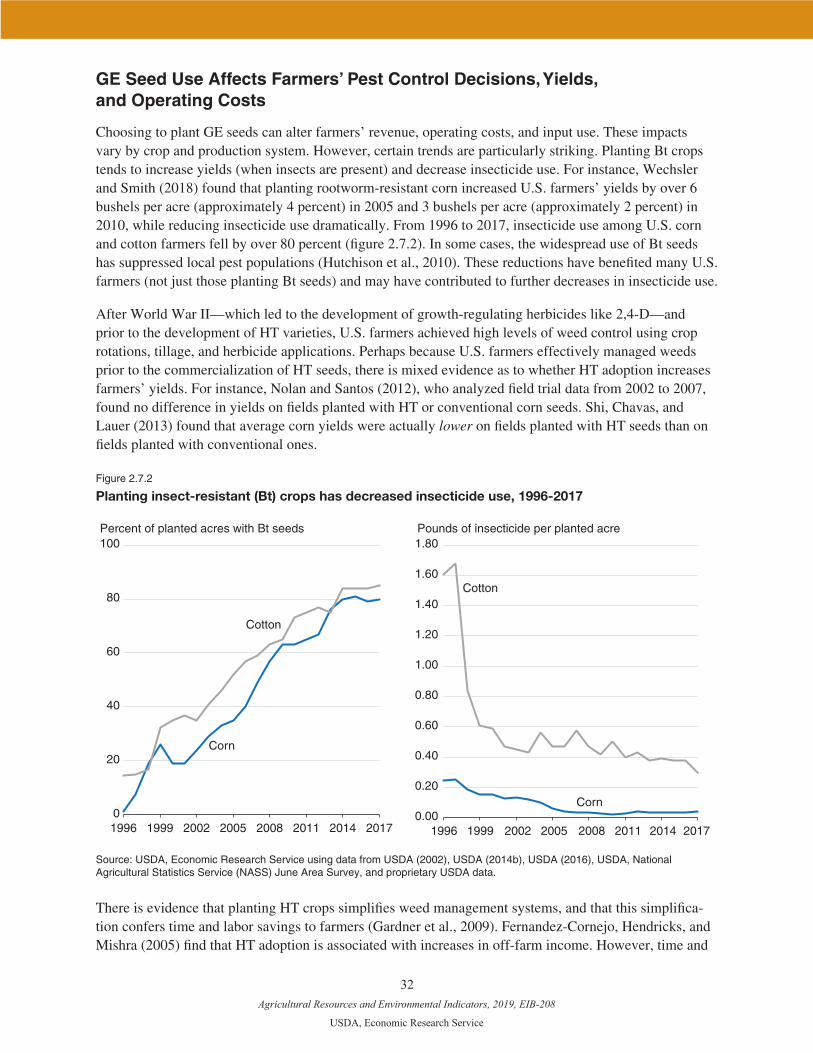
Agricultural Resources and Environmental Indicators, 2019, EIB-208
USDA, Economic Research Service
32
GE Seed Use Affects Farmers’ Pest Control Decisions, Yields, and Operating Costs
Choosing to plant GE seeds can alter farmers’ revenue, operating costs, and input use. These impacts vary by crop and production system. However, certain trends are particularly striking. Planting Bt crops tends to increase yields (when insects are present) and decrease insecticide use. For instance, Wechsler and Smith (2018) found that planting rootworm-resistant corn increased U.S. farmers’ yields by over 6 bushels per acre (approximately 4 percent) in 2005 and 3 bushels per acre (approximately 2 percent) in 2010, while reducing insecticide use dramatically. From 1996 to 2017, insecticide use among U.S. corn and cotton farmers fell by over 80 percent (figure 2.7.2). In some cases, the widespread use of Bt seeds has suppressed local pest populations (Hutchison et al., 2010). These reductions have benefited many U.S. farmers (not just those planting Bt seeds) and may have contributed to further decreases in insecticide use.
After World War II—which led to the development of growth-regulating herbicides like 2,4-D—and prior to the development of HT varieties, U.S. farmers achieved high levels of weed control using crop rotations, tillage, and herbicide applications. Perhaps because U.S. farmers effectively managed weeds prior to the commercialization of HT seeds, there is mixed evidence as to whether HT adoption increases farmers’ yields. For instance, Nolan and Santos (2012), who analyzed field trial data from 2002 to 2007, found no difference in yields on fields planted with HT or conventional corn seeds. Shi, Chavas, and Lauer (2013) found that average corn yields were actually lower on fields planted with HT seeds than on fields planted with conventional ones.
Figure 2.7.2
Planting insect-resistant (Bt) crops has decreased insecticide use, 1996-2017
Percent of planted acres with Bt seeds Pounds of insecticide per planted acre
0
20
40
60
80
100
1996 1999 2002 2005 2008 2011 2014 20170.00
0.20
0.40
0.60
0.80
1.00
1.20
1.40
1.60
1.80
1996 1999 2002 2005 2008 2011 2014 2017
Corn
Corn
Cotton
Cotton
Source: USDA, Economic Research Service using data from USDA (2002), USDA (2014b), USDA (2016), USDA, National Agricultural Statistics Service (NASS) June Area Survey, and proprietary USDA data.
There is evidence that planting HT crops simplifies weed management systems, and that this simplifica-tion confers time and labor savings to farmers (Gardner et al., 2009). Fernandez-Cornejo, Hendricks, and Mishra (2005) find that HT adoption is associated with increases in off-farm income. However, time and
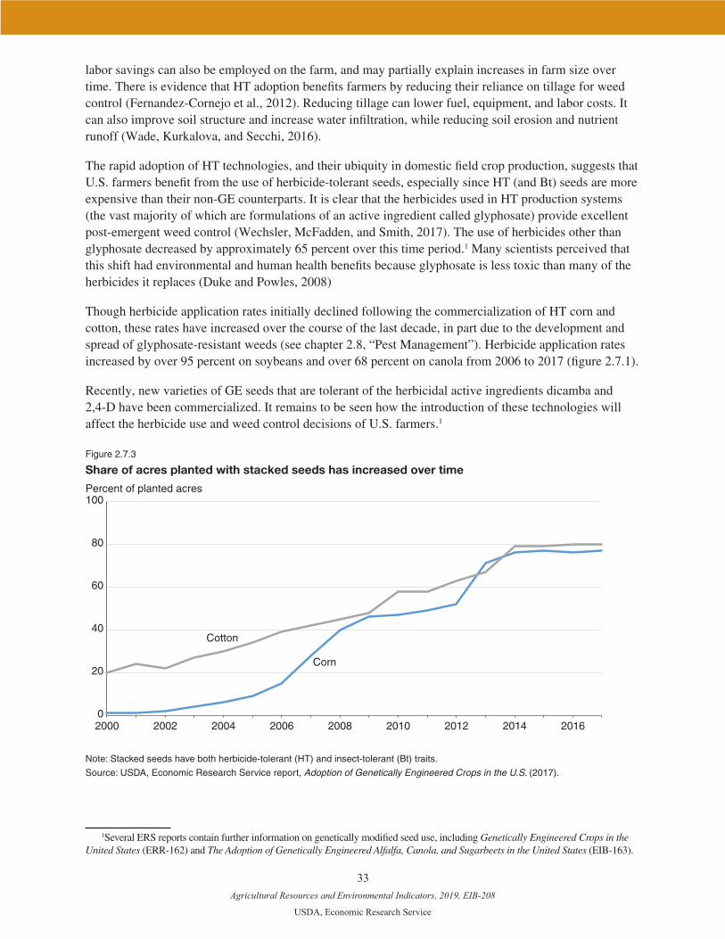
Agricultural Resources and Environmental Indicators, 2019, EIB-208
USDA, Economic Research Service
33
labor savings can also be employed on the farm, and may partially explain increases in farm size over time. There is evidence that HT adoption benefits farmers by reducing their reliance on tillage for weed control (Fernandez-Cornejo et al., 2012). Reducing tillage can lower fuel, equipment, and labor costs. It can also improve soil structure and increase water infiltration, while reducing soil erosion and nutrient runoff (Wade, Kurkalova, and Secchi, 2016).
The rapid adoption of HT technologies, and their ubiquity in domestic field crop production, suggests that U.S. farmers benefit from the use of herbicide-tolerant seeds, especially since HT (and Bt) seeds are more expensive than their non-GE counterparts. It is clear that the herbicides used in HT production systems (the vast majority of which are formulations of an active ingredient called glyphosate) provide excellent post-emergent weed control (Wechsler, McFadden, and Smith, 2017). The use of herbicides other than glyphosate decreased by approximately 65 percent over this time period.1 Many scientists perceived that this shift had environmental and human health benefits because glyphosate is less toxic than many of the herbicides it replaces (Duke and Powles, 2008)
Though herbicide application rates initially declined following the commercialization of HT corn and cotton, these rates have increased over the course of the last decade, in part due to the development and spread of glyphosate-resistant weeds (see chapter 2.8, “Pest Management”). Herbicide application rates increased by over 95 percent on soybeans and over 68 percent on canola from 2006 to 2017 (figure 2.7.1).
Recently, new varieties of GE seeds that are tolerant of the herbicidal active ingredients dicamba and 2,4-D have been commercialized. It remains to be seen how the introduction of these technologies will affect the herbicide use and weed control decisions of U.S. farmers.1
Figure 2.7.3
Share of acres planted with stacked seeds has increased over time
Percent of planted acres
0
20
40
60
80
100
2000 2002 2004 2006 2008 2010 2012 2014 2016
Cotton
Corn
Note: Stacked seeds have both herbicide-tolerant (HT) and insect-tolerant (Bt) traits.
Source: USDA, Economic Research Service report, Adoption of Genetically Engineered Crops in the U.S. (2017).
1Several ERS reports contain further information on genetically modified seed use, including Genetically Engineered Crops in the United States (ERR-162) and The Adoption of Genetically Engineered Alfalfa, Canola, and Sugarbeets in the United States (EIB-163).

Agricultural Resources and Environmental Indicators, 2019, EIB-208
USDA, Economic Research Service
34
References
Brookes, G. 2014. “Weed control changes and genetically modified herbicide tolerant crops in the USA 1996-2012,” GM Crops Food 5(4): 321-332.
Duke, S., and S. Powles. 2008. “Glyphosate: A Once-In-A-Century Herbicide,” Pest Management Science 65:319-325.
Fernandez-Cornejo, J., C. Hallahan, R. Nehring, and S. Wechsler. 2012. “Conservation Tillage, Herbicide Use, and Genetically Engineered Crops in the United States: The Case of Soybeans,” AgBioForum 15(3): 231-241.
Fernandez-Cornejo, J., C. Hendricks, and A. Mishra. 2005. “Technology Adoption and Off-Farm House-hold Income: The Case of Herbicide-Tolerant Soybeans,” Journal of Agricultural and Applied Eco-nomics 37(3): 549-563.
Fernandez-Cornejo, J. and W. McBride. 2002. Adoption of Bioengineered Crops. U.S. Department of Agriculture, Economic Research Service.
Fernandez-Cornejo, J., R. Nehring, C. Osteen, S. Wechsler, A. Martin, and A. Vialou. 2014. Pesticide Use in U.S. Agriculture: 21 Selected Crops, 1960-2008. U.S. Department of Agriculture, Economic Re-search Service.
Fernandez-Cornejo, J., S. Wechsler, M. Livingston, and L. Mitchell. 2014. Genetically Engineered Crops in the United States. U.S. Department of Agriculture, Economic Research Service.
Fernandez-Cornejo, J., S. Wechsler, and D. Milkove. 2016. The Adoption of Genetically Engineered Alfal-fa, Canola, and Sugarbeets in the United States. USDA, Economic Research Service, Washington, DC.
Gardner, J., R. Nehring, and C. Nelson. 2009. “Genetically Modified Crops and Household Labor Savings in US Crop Production,” AgBioForum 12(3-4): 303-312.
Hutchison W., E. Burkness, D. Mitchell, R. Moon, T. Leslie, S. Fleischer, M. Abrahamson, K. Hamilton, K. Steffey, M. Gray, R. Hellmich, L. Kaster, T. Hunt, R. Wright, K. Pecinovsky, T. Rabaey, B. Flood, and E. Raun. 2010. “Areawide Suppression of European Corn Borer with Bt Maize Reaps Savings to Non-Bt Maize Growers,” Science 330 (6001): 222-225.
Livingston, M., J. Fernandez-Cornejo, J. Unger, C. Osteen, D. Schimmelpfennig, T. Park, and D. Lam-bert. 2015. The Economics of Glyphosate Resistance Management in Corn and Soybean Production. U.S. Department of Agriculture, Economic Research Service.
Nolan, E., and P. Santos. 2012. “The Contribution of Genetic Modification to Changes in Corn Yield in the United States,” American Journal of Agricultural Economics 94 (5): 1171-88.
Shi, G., J.P. Chavas, and J. Lauer. 2013. “Commercialized transgenic traits, maize productivity and yield risk,” Nature Biotechnology 31(2): 111-114.
U.S. Department of Agriculture, National Agricultural Statistics Service. 2016. June Area Survey. Wash-ington, DC.
Wade, T., L. Kurkalova, and S. Secchi. 2016. “Modeling Field-Level Conservation Tillage Adoption with Aggregate Choice Data,” Journal of Agricultural and Resource Economics 41(2): 266-285.
Wechsler, S. 2018. Adoption of Genetically Engineered Crops in the U.S. [Online]. USDA, Economic Research Service, Washington, DC.
Wechsler, S., J. McFadden, and D. Smith. 2017. “What do farmers’ weed control decisions imply about glyphosate resistance? Evidence from surveys of US corn fields,” Pest Management Science 74(5): 1143-1154.
Wechsler, S., and D. Smith. 2018. “Has Resistance Taken Root in U.S. Corn Fields? Demand for Insect Control,” American Journal of Agricultural Economics 100(4): 1136-1150.

Agricultural Resources and Environmental Indicators, 2019, EIB-208
USDA, Economic Research Service
35
Chapter 2.8—Pest Management
Richard Nehring
• In 2012, U.S. producers spent over $9 billion on pesticides to control pests such as insects, mites, and weeds.
• The development of herbicide resistance in several weed species has contributed to increased recent herbicide use. From 2010 to 2014, herbicide application rates (per planted acre) rose by 24 percent on U.S. soybeans, 26 percent on wheat, 25 percent on cotton, and 21 percent on corn.
• Weed resistance to newer herbicides has led to expanded use of some older herbicides.
Pests—such as insects, mites, and weeds—can reduce crop yields or the quality of production, while the cost of managing pests can reduce farm profitability. To control pests, farmers rely on pesticides like herbicides, insecticides, and fungicides; pesticides also include soil fumigants, plant growth regulators, defoliants, and desiccants. Pesticides can be synthetic (developed in laboratories and manufactured) or natural (chemical compounds occurring in nature).
Pesticide Trends
According to U.S. Environmental Protection Agency (EPA) data, U.S. agricultural producers spent over $9 billion on 899 million pounds of pesticide active ingredient in 2012. That was about 32 percent more (in inflation-adjusted terms) than was spent in 2007, and 10 percent more pounds of pesticide active ingre-dient.1 Between 2007 and 2012, herbicide expenditures declined from 62 to 59 percent of total pesticide expenditures, but the share of total applied active ingredient weight accounted for by herbicides increased from 54 to 63 percent (see fig. 2.8.1).
U.S. corn, cotton, fall potatoes, soybeans, and wheat account for nearly two-thirds of pesticide quantities applied.2 Total pesticide applications on these five crops, which fluctuated between approximately 400 and 500 million pounds in the 1980s and 1990s, rose sharply after 2005 and reached 634 million pounds in 2014 (fig. 2.8.2).3
Corn accounted for 46 percent of all pesticides (by weight) applied to the five major crops in 2014, and hence nearly one-third of all pesticide applications. The second largest crop, soybeans, accounted for another 31 percent of pesticides applied in 2014.
1Throughout this chapter, we aim to use the latest data available for the selected series at the time the report was prepared. Because of changes in the data sources and methodology used in EPA source documents, pesticide expenditures reported here for 2007 differ substantially from those reported for 2007 in the 2012 Agricultural Resources and Environmental Indicators report (USDA, Economic Research Service).
2Pesticide applications are often reported in pounds of active ingredient. The same quantities of different pesticides may have differing levels of toxicity, modes of action, target pests, and environmental impacts; hence, not all pounds are the same. None-theless, aggregated quantity data are widely reported and provide a useful base for tracking applications, while taking account of changes in pesticide attributes.
3These estimates do not include sulfur, oils, and unconventional pesticides such as biological or microbial pesticides.
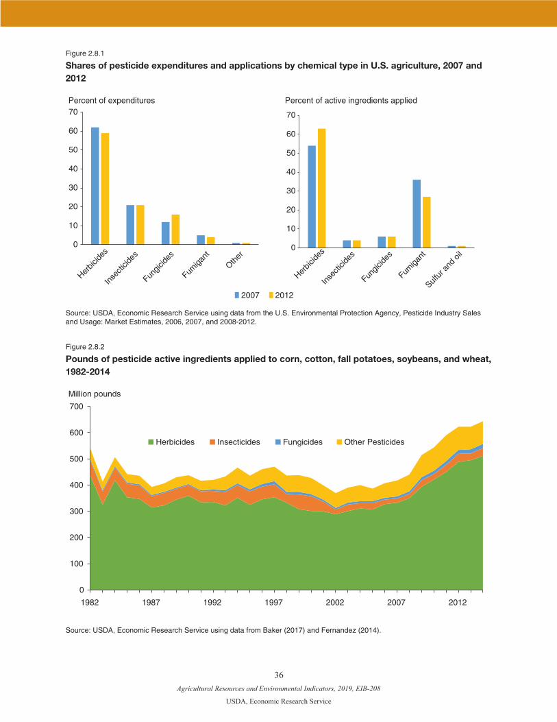
Agricultural Resources and Environmental Indicators, 2019, EIB-208
USDA, Economic Research Service
36
Figure 2.8.1
Shares of pesticide expenditures and applications by chemical type in U.S. agriculture, 2007 and 2012
Percent of expenditures Percent of active ingredients applied
0
10
20
30
40
50
60
70
Herbic
ides
Inse
cticid
es
Fungic
ides
Fumiga
nt
Other
2007 2012
0
10
20
30
40
50
60
70
Herbic
ides
Inse
cticid
es
Fungic
ides
Fumiga
nt
Sulfur
and
oil
Source: USDA, Economic Research Service using data from the U.S. Environmental Protection Agency, Pesticide Industry Sales and Usage: Market Estimates, 2006, 2007, and 2008-2012.
Figure 2.8.2
Pounds of pesticide active ingredients applied to corn, cotton, fall potatoes, soybeans, and wheat, 1982-2014
Million pounds
0
100
200
300
400
500
600
700
1982 1987 1992 1997 2002 2007 2012
Herbicides Insecticides Fungicides Other Pesticides
Source: USDA, Economic Research Service using data from Baker (2017) and Fernandez (2014).
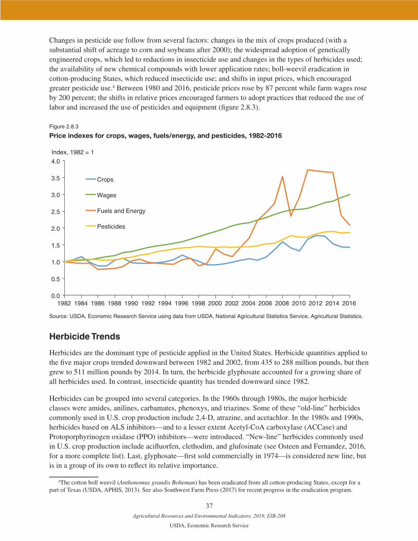
Agricultural Resources and Environmental Indicators, 2019, EIB-208
USDA, Economic Research Service
37
Changes in pesticide use follow from several factors: changes in the mix of crops produced (with a substantial shift of acreage to corn and soybeans after 2000); the widespread adoption of genetically engineered crops, which led to reductions in insecticide use and changes in the types of herbicides used; the availability of new chemical compounds with lower application rates; boll-weevil eradication in cotton-producing States, which reduced insecticide use; and shifts in input prices, which encouraged greater pesticide use.4 Between 1980 and 2016, pesticide prices rose by 87 percent while farm wages rose by 200 percent; the shifts in relative prices encouraged farmers to adopt practices that reduced the use of labor and increased the use of pesticides and equipment (figure 2.8.3).
Figure 2.8.3
Price indexes for crops, wages, fuels/energy, and pesticides, 1982-2016
Index, 1982 = 1
0.0
0.5
1.0
1.5
2.0
2.5
3.0
3.5
4.0
1982 1984 1986 1988 1990 1992 1994 1996 1998 2000 2002 2004 2006 2008 2010 2012 2014 2016
Crops
Wages
Fuels and Energy
Pesticides
Source: USDA, Economic Research Service using data from USDA, National Agricultural Statistics Service, Agricultural Statistics.
Herbicide Trends
Herbicides are the dominant type of pesticide applied in the United States. Herbicide quantities applied to the five major crops trended downward between 1982 and 2002, from 435 to 288 million pounds, but then grew to 511 million pounds by 2014. In turn, the herbicide glyphosate accounted for a growing share of all herbicides used. In contrast, insecticide quantity has trended downward since 1982.
Herbicides can be grouped into several categories. In the 1960s through 1980s, the major herbicide classes were amides, anilines, carbamates, phenoxys, and triazines. Some of these “old-line” herbicides commonly used in U.S. crop production include 2,4-D, atrazine, and acetachlor. In the 1980s and 1990s, herbicides based on ALS inhibitors—and to a lesser extent Acetyl-CoA carboxylase (ACCase) and Protoporphyrinogen oxidase (PPO) inhibitors—were introduced. “New-line” herbicides commonly used in U.S. crop production include acifluorfen, clethodim, and glufosinate (see Osteen and Fernandez, 2016, for a more complete list). Last, glyphosate—first sold commercially in 1974—is considered new line, but is in a group of its own to reflect its relative importance.
4The cotton boll weevil (Anthonomus grandis Boheman) has been eradicated from all cotton-producing States, except for a part of Texas (USDA, APHIS, 2013). See also Southwest Farm Press (2017) for recent progress in the eradication program.

Agricultural Resources and Environmental Indicators, 2019, EIB-208
USDA, Economic Research Service
38
Major factors affecting overall herbicide use trends since 1980 include:
1. Changes in crop acreage, influenced by economic and policy factors;
2. The replacement of older compounds with newer ones that are applied at lower per-acre rates;
3. The adoption of genetically engineered crops since the mid-1990s (see chapter 2.7, “Biotechnology, Seed Use, and Pest Control for Major U.S. Crops”); and
4. Evolution of herbicide resistance in weeds.
Changing Mix of Herbicide Types Used in the United States
Since new-line herbicides are generally applied at lower rates, their increasing use, together with declin-ing crop acreages through the late 1980s, contributed to declines in aggregate herbicide quantities applied between 1982 and 2002 (Osteen and Fernandez, 2016). The year 1996 saw the introduction of corn, cotton, and soybean seeds that were genetically engineered to be tolerant of the broad-spectrum herbicide glyphosate, sold under the Roundup label. This allowed farmers to spray the herbicide on field after the crop emerged, thus easing weed management for farmers. Glyphosate was quite effective at controlling a wide range of weeds; it was less environmentally damaging than old-line herbicides; and the herbicide’s price also fell sharply after it went off-patent in 2002. The expansion of corn, cotton, and soybean acres planted to glyphosate tolerant seeds accelerated rapidly, and led to the displacement of other herbicides by glyphosate. Glyphosate use in the U.S. agricultural sector increased sevenfold between 1995 (the year before glyphosate-tolerant seeds were introduced) and 2014.
Heavy reliance on a single mode of weed control encourages the spread of weeds that are resistant to that mode, as resistant individual weeds survive and propagate (Livingston et al., 2015; Owen, 2015). The heavy, and often exclusive, reliance on glyphosate in many areas led to the rapid emergence and spread of glyphosate-resistant weeds, but there is evidence that weeds are developing resistance to other herbicides as well (Heap, 2015; Owen, 2015).
Farmers responded to growing weed resistance by increasing their use of other old- and new-line herbi-cides, but also by increasing their application rates for glyphosate. (Peterson et al., 2018). From 2010 to 2014, glyphosate use increased by 41 million pounds, but use of old-line herbicides increased by 51 mil-lion pounds. By 2014, while glyphosate was still the largest-selling herbicide product, old-line herbicides as a group accounted for half of herbicide quantity applied. Application rates (for all herbicides) increased by 20 percent from 1.67 pounds per acre in 2010 to 1.92 pounds in 2014, reflecting more intensive use.
We can track the use of old-line herbicides, glyphosate, and other new line herbicides for the four major herbicide-using crops—corn, cotton, soybeans, and wheat. We illustrate the share of herbicide- treated acres receiving each kind of herbicide in figure 2.8.4 and the shares of each herbicide type in total herbi-cide applied (by weight) in figure 2.8.5. Finally, we track average application rates, per acre treated with herbicide, in figure 2.8.6.5
5Data on acre-treatments for figure 2.8.4 are drawn from USDA, National Agricultural Statistics Service data, while those in figures 2.8.5 and 2.8.6 are drawn from U.S. Geological Survey data. The dates of the most recent data available differ by source.

Agricultural Resources and Environmental Indicators, 2019, EIB-208
USDA, Economic Research Service
39
Several patterns stand out:
• Glyphosate was used more widely and intensively in soybeans than in corn, cotton, or wheat (figure 2.8.4 and figure 2.8.5).
• All four crops show a decline in the share of acres treated with glyphosate in recent years: after 2010 (corn and cotton) or 2012 (soybeans and wheat, figure 2.8.4).
• Looking at shares of herbicides applied by weight (fig. 2.8.5), the prevalence of glyphosate use increased slightly for corn, rose for wheat, and fell for cotton and soybeans in the most recent year for which data were available.
• Old-line herbicides increased their share of total pounds applied for both cotton and soybeans, sta-bilized in corn, and decreased in wheat (figure 2.8.5).
• Application rates increased persistently for each of the four crops after 2002 (figure 2.8.6).
Figure 2.8.4
Shares of herbicide type applied (old line/new line/glyphosate) on herbicide-treated acres, by crop and year, 2002-2016
0
10
20
30
40
50
60
70
80
90
100
2002 2010 2016 2002 2010 2015 2002 2012 2015 2002 2012 2015
Old-line treatment acres New-line treatment acres Glyphosate treatment acres
Cotton Wheat SoybeansCorn
Note: Years displayed reflect years of survey data availability, which vary by crop. The final year of data displayed (2016 for corn, and 2015 for cotton, wheat, and soybeans) reflects the latest USDA NASS survey years for that crop. Old-line herbicides were in families first observed in the 1964, 1966, or 1971 surveys; glyphosate was first observed in the 1976 survey; and new-line herbi-cides were in families or modes of action (MOAs) first observed in the 1976 or later surveys (Fernandez and Osteen, 2016).Source: USDA Economic Research Service using data from USDA, National Agricultural Statistics Service (NASS), Quick Stats.
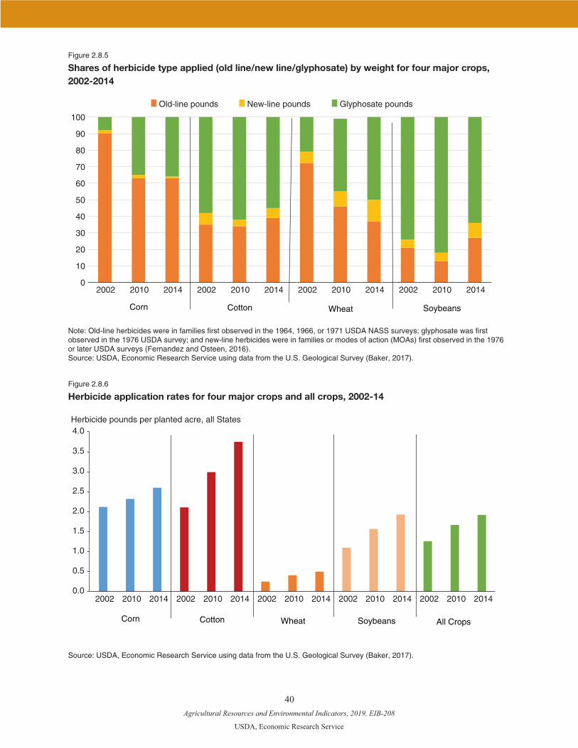
Agricultural Resources and Environmental Indicators, 2019, EIB-208
USDA, Economic Research Service
40
Figure 2.8.5
Shares of herbicide type applied (old line/new line/glyphosate) by weight for four major crops, 2002-2014
0
10
20
30
40
50
60
70
80
90
100
2002 2010 2014 2002 2010 2014 2002 2010 2014 2002 2010 2014
Old-line pounds New-line pounds Glyphosate pounds
Corn Cotton Wheat Soybeans
Note: Old-line herbicides were in families first observed in the 1964, 1966, or 1971 USDA NASS surveys; glyphosate was first observed in the 1976 USDA survey; and new-line herbicides were in families or modes of action (MOAs) first observed in the 1976 or later USDA surveys (Fernandez and Osteen, 2016). Source: USDA, Economic Research Service using data from the U.S. Geological Survey (Baker, 2017).
Figure 2.8.6
Herbicide application rates for four major crops and all crops, 2002-14
0.0
0.5
1.0
1.5
2.0
2.5
3.0
3.5
4.0
2002 2010 2014 2002 2010 2014 2002 2010 2014 2002 2010 2014 2002 2010 2014
Herbicide pounds per planted acre, all States
Corn Cotton Wheat Soybeans All Crops
Source: USDA, Economic Research Service using data from the U.S. Geological Survey (Baker, 2017).

Agricultural Resources and Environmental Indicators, 2019, EIB-208
USDA, Economic Research Service
41
Summary
Herbicides account for the vast majority of pesticide applications by U.S. farmers. Patterns of herbicide use have shifted in recent years. Total application of herbicides has increased in the last decade, after showing little trend for nearly 25 years. The resurgence of old-line herbicides is evident as producers struggle with herbicide resistance in weeds caused by recurring use of the same chemicals, such as glyphosate (Arp, 2017). In short, herbicide-use patterns differ by crop, with variations in the mix of old-line and new-line (including glyphosate) herbicide use driven by weed resistance and other factors.
References
Arp, Allison. 2017. “Herbicide Resistance, the Catalyst of the Growing Problem,” Iowa Soybean Review, February.
Baker, N.T. 2017. “Estimated annual agricultural pesticide use by crop group for states of the contermi-nous United States, 1992-2014.” U.S. Geological Survey data release.
Fernandez-Cornejo, Jorge, Richard Nehring, Craig Osteen, Seth Wechsler, Alex Vialou, and Arthur Grube. 2014. Trends in Pesticide Use in U.S. Agriculture, 1960-2008. U.S. Department of Agriculture, Eco-nomic Research Service. EIB-124, April.
Heap, I. 2016. “The International Survey of Herbicide Resistant Weeds.” Hugie, Josie A., German A. Bolero, Patrick J. Tranel, and Dean E. Riechers. 2008. “The Rate Require-
ments for Synergism between Mesotrione and Atrazine in Fedroot Pigweed (Amaranthus retroflexus),” Weed Science 56, March-April.
Iowa State University Extension and Outreach. 2017. 2018 Herbicide Guide for Iowa Corn and Soybean Production Industry Update for 2018. Nov.
Livingston, Michael, Jorge Fernandez-Cornejo, Jesse Unger, Craig Osteen, David Schimmelpfennig, Tim Park, and Dayton Lambert. 2015. The Economics of Glyphosate Resistance Management in Corn and Soybean Production. U.S. Department of Agriculture, Economic Research Service. ERR-184 April.
National Research Council (NRC), Environmental Studies Board. 1975. Pest Control: An Assessment of Present and Alternative Technologies (Volume 1). Washington, DC: The National Academies Press.
Osteen, C.D., and J. Fernandez-Cornejo. 2016. “Herbicide Use Trends: A Backgrounder,” Choices. Quar-ter 4.
Owen, Michael D.K., Hugh J. Beckie, Julia Y. Leeson, Jason K. Norsworthy, and Larry E. Steckel. 2015. “Integrated Pest Management and Weed Management in the United States and Canada,” Pest Manage-ment Science 64.
Peterson, Mark, Alberto Collavo, Ramiro Ovejero, Vinod Shivraind, and Michael J. Walshe. 2017. “The challenge of herbicide resistance around the world: a current summary,” Pest Management Science 74.
Southwest Farm Press. 2017. “After years of challenges, boll weevil eradication program making prog-ress.”
U.S. Department of Agriculture, Animal and Plant Health Inspection Service. 2013. FactSheet, Plant Protection and Quarantine.
U.S. Department of Agriculture, National Agricultural Statistics Service. Agricultural Statistics, selected issues.
U.S. Department of Agriculture, National Agricultural Statistics Service. 2011 - 2015. Acreage. U.S. Department of Agriculture, National Agricultural Statistics Service. Quick Stats Chemical Use Sur-
veys, 1990 to 2017.

Agricultural Resources and Environmental Indicators, 2019, EIB-208
USDA, Economic Research Service
42
Chapter 2.9—Nutrient Management
Roberto Mosheim
• Commercial fertilizer consumption was about 22 million short tons in 2015, recovering from the 18-percent drop between 2008 and 2009.
• Since 1997, nitrogen recovery rates (the share of applied nutrient taken up by the harvested crop) on corn, winter wheat, and cotton have hovered around 70 percent, while recovery rates for phosphate have remained around 60 percent.
• The shares of planted acreage where application rates exceed 125 percent of the crop’s agronomic need (a measure of nutrient overapplication) have decreased for both nitrogen and phosphate.
This chapter examines the key technological and economic drivers of plant nutrient consumption and trends in nutrient use efficiency.1 There is a complex interaction between fertilizer use and subsequent benefits and costs. On the one hand, crop plants require inorganic nutrients such as nitrogen, potash, and phosphate for crop production. On the other hand, excessive application of nutrients can damage air and water resources through soil erosion, runoff, volatilization, and leaching (Ribaudo et al., 2011).
When fertilizer applications are warranted for crops, the application of excess nutrients can be reduced by implementing what USDA’s Natural Resources Conservation Service2 and The Fertilizer Institute promote as the 4Rs. The 4Rs direct farmers to apply nutrients using the right source of nutrients (matching fertilizer type to crop needs), at the right rate (matching amount of required fertilizer(s) to crop needs), at the right time (making nutrients available when crops need them most), and in the right place (applying nutrients where crops can use them) (The Fertilizer Institute, 2017). The 4Rs can increase prof-itability—by reducing fertilizer expenses and by better targeting its use to raise yields—and reduce the undesirable environmental impacts of excessive nutrient use.3
Variability in the Use of Nutrients
Commercial fertilizer use surged from 7.46 million short tons4 in 1960 to a peak of 23.68 million short tons in 1981 (figure 2.9.1). Total commercial fertilizer consumption of nitrogen, phosphate, and potash increased as more acres were devoted to high-yield crop varieties and as developed hybrids responded well to more intensive use of commercial fertilizer (EPA, 2017b).
Total applications of nitrogen, phosphate, and potash use on corn, soybeans, and wheat increased from 1964 to 1981 but declined for cotton. The expansion of total nutrient use through 1981 reflects expanded acreage (except cotton acreage, which fell slightly), increases in application rates, and a higher share of acres receiving fertilizer. This long expansion in fertilizer use ended in 1982. Since then, fertilizer use has
1Data sources include the most current data from USDA-ERS Fertilizer Use and Price data products, based on “Commercial Fertilizers, 2015” published in October 2018, and the latest commodity-specific Phase II surveys—corn, 2016; cotton, 2015; soybeans, 2012; and winter wheat, 2017.
2See, for example, USDA Natural Resources Conservation Service’s (2013) Nutrient Management Practice Standard 590.3The implementation of the 4Rs conforms with precision agriculture. For example, Schimmelpfennig (2016), Snyder (2016),
and Bruulsema (2017) examine technologies such as global positioning system (GPS) mapping, grid or zone soil sampling, yield monitors, and variable-rate technology (VRT) that can improve nutrient use and reduce environmental risk (see chapter 2.11, “Precision Agriculture”).
4One short ton = 2,000 pounds.

Agricultural Resources and Environmental Indicators, 2019, EIB-208
USDA, Economic Research Service
43
fluctuated over time in line with changes in cropping system implementation and fertilizer/crop prices, but has shown no persistent trend.
Figure 2.9.1
Total nutrient use increased dramatically until 1981
Short tons (millions)
0
5
10
15
20
25
1960 1966 1972 1978 1984 1990 1996 2002 2008 2014
Nitrogen
Phosphate
Potash
Total
Note: 1 short ton equals 2,000 pounds. Source: USDA, Economic Research Service using data from the Tennessee Valley Authority, Association of American Plant Food Control officials (2018).
Lower fertilizer prices generally meant increased fertilizer use until the energy crisis of 1973, when fertil-izer prices jumped temporarily to their highest level ever. Still, nutrient use kept increasing (figure 2.9.2).5 Commercial fertilizer prices slid until 2002, when they bottomed out at $247 per ton—historically, the lowest (inflation-adjusted) average fertilizer price for which data are available. Since 2002, fertilizer prices have fluctuated significantly, with no clear effect on fertilizer use.
Domestic fertilizer demand does not affect fertilizer price, but global events in energy markets do. For example, movements in key fertilizer feedstock prices like natural gas affect fertilizer prices and, in turn, demand. A key event, the global economic crisis of 2008/2009, put downward pressure on natural gas prices, which in turn reduced fertilizer prices. Fertilizer prices fell 18 percent from 2008 to 2009 (fig. 2.9.2) and fertilizer use dropped 14 percent because of reduced global incomes.6 By 2015, fertilizer use and price were back to pre-crisis levels. Fertilizer prices have fallen relative to 2015, but nitrogen fertilizer prices appear to have stabilized thus far in 2018 (Schnitkey, 2017 and 2018).
5USDA-ERS constructed a price index for fertilizer using the prices (see USDA-NASS, Agricultural Prices, 2017) of anhydrous ammonia, urea 44-46 percent nitrogen, ammonium nitrate, sulfate of ammonium, and super-phosphate 44-46 percent phosphate. USDA-NASS stopped publishing these prices in 2015. The price data were deflated by the Consumer Price Index (2016 = 100).
6 Shane et al. (2009) document the effects of the 2008/2009 world economic crisis on U.S. agriculture.

Agricultural Resources and Environmental Indicators, 2019, EIB-208
USDA, Economic Research Service
44
An increase in natural gas production came after the ascendancy of horizontal drilling and hydraulic fracturing in the United States—in October 2011, hydraulically fractured wells became the predominant method for new United States oil and gas development (EIA, 2018). In turn, the increase in the supply of this crucial raw material in the manufacture of nitrogen fertilizer put downward pressure on fertilizer prices at the cost, however, of an increased risk of environmentally damaging drinking water resources (EPA, 2016).
The above interactions between fertilizer prices and quantity are important from an environmental per-spective. For example, how responsive is fertilizer demand to movements in fertilizer price? The literature (Roberts and Heady, 1982; Yang and Shumway, 2015) finds that the sensitivity of fertilizer demand to fer-tilizer price is very small (within its historic price ranges). Meanwhile, domestic fertilizer prices are high-ly dependent on prices determined in the international market, including the price of natural gas, a crucial raw material in the manufacture of ammonia, which in turn is fundamental to inorganic nitrogen fertilizer. Weak demand response to price affects implementation of best practices in the application of fertilizer and influences policies designed to contain the environmental damage from the overapplication of nutrients.
Figure 2.9.2
Fertilizer prices rose rapidly between 2002 and 2008
Short tons (million)
0
125
250
375
500
625
0
5
10
15
20
25
1960 1966 1972 1978 1984 1990 1996 2002 2008 2014
Fertilizer use
Fertilizer price
$/ton (2016)
Note: Data adjusted for inflation to 2016 dollars using the Consumer Price Index. Fertilizer price and use moved in opposite direc-tions until 1973. That is, between 1960 and 1973, fertilizer use expanded, partly in response to longrun price declines. Since 1973, movements in key fertilizer feedstock prices determined by global energy markets have been the main drivers of fertilizer prices. Fertilizer use is very insensitive to movements in fertilizer price. Prices increased 43 percent from 2007 to 2008, and use decreased 18 percent following the 2008-09 financial crisis.Source: USDA, Economic Research Service analysis of data from the Tennessee Valley Authority, the Association of Plant Food Control Officials, and the Fertilizer Institute.

Agricultural Resources and Environmental Indicators, 2019, EIB-208
USDA, Economic Research Service
45
Nutrient Recovery Rates Remain Constant for Most Crops
A well-designed nutrient management plan decreases nutrient expenses and lowers the environmental impact of nutrient use. Nutrient recovery is the ratio of the amount of nutrient in the harvested crop to the amount of nutrient applied (Huang and Beckman, 2012). Partial recovery occurs when the amount applied exceeds the amount that plants can absorb, resulting in environmental loss. The partial recovery index varies between 0 and 100, with 0 being the least efficient and 100 being the most efficient use of applied nutrients. Figures 2.9.3 and 2.9.4 show nitrogen and phosphate recovery ratios for corn, winter wheat, cotton and soybeans.7 For corn, nitrogen efficiency increased from 58 percent in 1997 to 76 per-cent in 2015; for winter wheat, it increased from 56 percent in 1997 to 71 percent in 2016; for cotton, it increased from 58 percent in 1997 to 68 percent in 2014; and for soybeans it increased from 43 percent to 46 percent between 2005 and 2011.8 Phosphate recovery increased from 60 percent in 1997 to 65 percent in 2015 for corn, but decreased from 64 percent (1997) to 60 percent (2016) for winter wheat. For cotton, phosphorus recovery increased from 58 percent in 1997 to 66 percent in 2014, with much variability in between. Phosphate recovery for soybeans fell from 74 percent in 2005 to 58 percent in 2011. This last result, however, is based on only 2 years of observations. Nutrient use efficiency increases can be tied to the improved varieties of crops being grown—ones that have been bred for higher nutrient use efficien-cies—as well as to improved crop management practices that enable more efficient uptake of the applied nutrients (e.g., more farmers are following the 4Rs).
Figure 2.9.3
Crop’s nitrogen recovery rates
Percent of nitrogen applied
40
45
50
55
60
65
70
75
80
1997 1999 2001 2003 2005 2007 2009 2011 2013 2015
Corn Winter Wheat Cotton Soybeans
Source: USDA, Economic Research Service and National Agricultural Statistics Service, Agricultural Resource Management Survey (ARMS), Financial and Crop Production Practices.
7Nutrients employed in these crops represented about 60 percent of the total amount of nutrients consumed in the United States. Available data were employed to generate comparable variables across time to generate meaningful nutrient trends. Also, 2000 was the last year when nutrient use data were collected for corn, soybeans, cotton, and wheat at the same time. Winter wheat production is about 10 percent of total wheat production.
8Mourtzinis et al. (2018) conclude that nitrogen (N) management decisions have a measurable, but small, effect on soybean yield and that given the growing pressure for increasing food production, it is imperative to further examine all soybean N deci-sions (application method, timing, and rate) in terms of environmental and cropping system aspects.
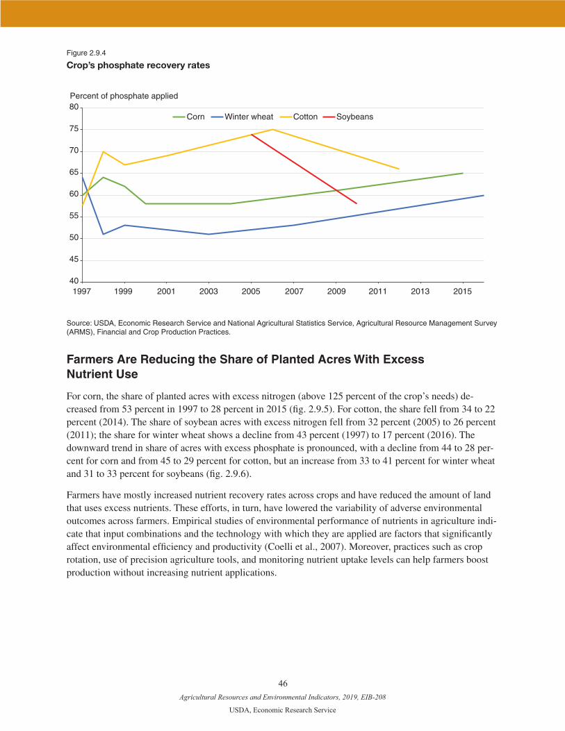
Agricultural Resources and Environmental Indicators, 2019, EIB-208
USDA, Economic Research Service
46
Figure 2.9.4
Crop’s phosphate recovery rates
Percent of phosphate applied
40
45
50
55
60
65
70
75
80
1997 1999 2001 2003 2005 2007 2009 2011 2013 2015
Corn Winter wheat Cotton Soybeans
Source: USDA, Economic Research Service and National Agricultural Statistics Service, Agricultural Resource Management Survey (ARMS), Financial and Crop Production Practices.
Farmers Are Reducing the Share of Planted Acres With Excess Nutrient Use
For corn, the share of planted acres with excess nitrogen (above 125 percent of the crop’s needs) de-creased from 53 percent in 1997 to 28 percent in 2015 (fig. 2.9.5). For cotton, the share fell from 34 to 22 percent (2014). The share of soybean acres with excess nitrogen fell from 32 percent (2005) to 26 percent (2011); the share for winter wheat shows a decline from 43 percent (1997) to 17 percent (2016). The downward trend in share of acres with excess phosphate is pronounced, with a decline from 44 to 28 per-cent for corn and from 45 to 29 percent for cotton, but an increase from 33 to 41 percent for winter wheat and 31 to 33 percent for soybeans (fig. 2.9.6).
Farmers have mostly increased nutrient recovery rates across crops and have reduced the amount of land that uses excess nutrients. These efforts, in turn, have lowered the variability of adverse environmental outcomes across farmers. Empirical studies of environmental performance of nutrients in agriculture indi-cate that input combinations and the technology with which they are applied are factors that significantly affect environmental efficiency and productivity (Coelli et al., 2007). Moreover, practices such as crop rotation, use of precision agriculture tools, and monitoring nutrient uptake levels can help farmers boost production without increasing nutrient applications.
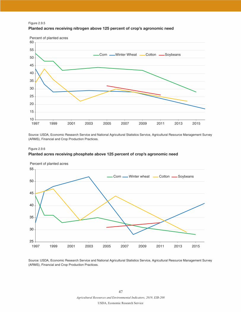
Agricultural Resources and Environmental Indicators, 2019, EIB-208
USDA, Economic Research Service
47
Figure 2.9.5
Planted acres receiving nitrogen above 125 percent of crop’s agronomic need
Percent of planted acres
10
15
20
25
30
35
40
45
50
55
60
1997 1999 2001 2003 2005 2007 2009 2011 2013 2015
Corn Winter Wheat Cotton Soybeans
Source: USDA, Economic Research Service and National Agricultural Statistics Service, Agricultural Resource Management Survey (ARMS), Financial and Crop Production Practices.
Figure 2.9.6
Planted acres receiving phosphate above 125 percent of crop’s agronomic need
Percent of planted acres
25
30
35
40
45
50
55
1997 1999 2001 2003 2005 2007 2009 2011 2013 2015
Corn Winter wheat Cotton Soybeans
Source: USDA, Economic Research Service and National Agricultural Statistics Service, Agricultural Resource Management Survey (ARMS), Financial and Crop Production Practices.

Agricultural Resources and Environmental Indicators, 2019, EIB-208
USDA, Economic Research Service
48
References
Association of American Plant Food Control Officials and the Fertilizer Institute. 2018. “Commercial Fertilizers 2015.”
Bruulsema, T. 2017. “4R Phosphorus Management Practices for Major Commodity Crops of North Amer-ica,” Issue Review Ref # 17023. International Plant Nutrition Institute.
Coelli, T., L. Lauwers, and G. Van Huylenbroeck. 2007. “Environmental efficiency measurement and the material balance condition,” Journal of Productivity Analysis 28.
Huang, W., and J. Beckman. 2012. “Nutrient Management,” Agricultural Resources and Environmental Indicators, 2012, EIB-98, U.S. Department of Agriculture, Economic Research Service, August.
Livingston, M., M. Roberts, and Y. Zhang. 2015. “Optimal Sequential Plantings of Corn and Soybeans Under Price Uncertainty,” American Journal of Agricultural Economics 97(3).
Mourtzinis, S., G. Kaur, J. Orlowski, C. Shapiro, C. Lee, C. Wortmann, D. Holshouser, E. Nafziger, H. Kandel, J. Niekamp, W. Ross, J. Lofton, J. Vonk, K. Roozeboom, K. Thelen, L. Lindsey, M. Staton, S. Naeve, S. Casteel, W. Wiebold, and S. Conley. 2018. “Soybean response to nitrogen application across the United States: A synthesis-analysis,” Field Crops Research 215.
Ribaudo, M., J. Delgado, L. Hansen, M. Livingston, R. Mosheim, and J. Williamson. 2011. Nitrogen in Agricultural Systems: Implications for Conservation Policy. ERR-127, U.S. Department of Agricul-ture, Economic Research Service, Sept.
Roberts, R.K., and E.O. Heady. 1982. “Fertilizer Demand Functions for Specific Nutrients Applied to Three Major U.S. Crops,” Western Journal of Agricultural Economics 7 (2): 265-277.
Schimmelpfennig, D. 2016. Farm Profits and Adoption of Precision Agriculture. ERR-217. U.S. Department of Agriculture, Economic Research Service, Oct.
Schnitkey, G. 2017. “Fertilizer Costs in 2017 and 2018,” farmdoc daily (7). Department of Agricultural and Consumer Economics, University of Illinois at Urbana-Champaign, July 11.
Schnitkey, G. 2018. “Nitrogen Prices, Rates Cuts, and 2018 Fertilizer Costs.” farmdoc daily (8). Depart-ment of Agricultural and Consumer Economics, University of Illinois at Urbana-Champaign, April 3.
Shane, M., W. Liefert, M. Morehart, M. Peters, J. Dillard, D. Torgerson, and W. Edmondson. 2009. The 2008/2009 World Economic Crisis: What It Means for U.S. Agriculture. Special Outlook Report, WRS-09-02, U.S. Department of Agriculture, Economic Research Service, March.
Snyder, C. 2016. “Suites of 4R Nitrogen Management Practices of Sustainable Crop Production and Envi-ronmental Protection,” Issue Review Ref # 16057. International Plant Nutrition Institute.
The Fertilizer Institute. 2017. “What are the 4 Rs?” U.S. Department of Agriculture, Economic Research Service. 2017. “U.S. Fertilizer Use and Price.” U.S. Department of Agriculture. Natural Resources Conservation Service. 2013. “Conservation Practice
Standard Nutrient Management Code 590.”U.S. Department of Agriculture, National Agricultural Statistics Service. 2017. “Agricultural Prices.” U.S. Energy Information Administration (EIA). 2018. “Hydraulically fractured horizontal wells account
for most new oil and natural gas wells.” January 30. U.S. Environmental Protection Agency. 2016. “Hydraulic Fracturing for Oil and Gas: Impacts from the
Hydraulic Fracturing Water Cycle on Drinking Water Resources in the United States (Final Report).”U.S. Environmental Protection Agency. 2017a. “Agriculture: Nutrient Management and Fertilizer.” U.S. Environmental Protection Agency. 2017b. “Nutrient Pollution: Sources and Solutions. Agriculture.” Yang, S., and C.R. Shumway. 2015. “Dynamic Adjustment in U.S. Agriculture Under Climate Change,”
American Journal of Agricultural Economics 98(3).

Agricultural Resources and Environmental Indicators, 2019, EIB-208
USDA, Economic Research Service
49
Chapter 2.10—U.S. Irrigated Agriculture: Farm Structure, Technology, and Conservation
Glenn Schaible and Marcel Aillery
• Irrigated farms accounted for approximately 39 percent of U.S. farm sales for crop and livestock products and 50 percent of U.S. crop sales in 2012. Irrigation’s importance is significantly higher in the more arid Western States, where 72 percent of U.S. irrigated acres were located and where irrigated farms accounted for nearly 60 percent of the region’s farm sales and more than 70 percent of regional crop sales.
• Most U.S. irrigated farms (64 percent) were low-sales farms (under $150,000 in annual farm sales); however, large-scale farms ($1,000,000 or more) accounted for 60 percent of irrigated acres, 62 percent of farm water applied, and 79 percent of irrigated farm sales. Per-farm sales in the United States averaged $514,400 for irrigated farms and $133,600 for dryland-only farms.
• While irrigated agriculture has become more water-use efficient over time, future irrigation efficien-cy gains will depend increasingly on adoption of improved onfarm water-management practices in combination with high-efficiency irrigation application systems.
Irrigated agriculture relies heavily on the Nation’s water resources to provide an important contribution to the U.S. agricultural economy. Irrigation is the largest use of U.S. freshwater withdrawals (42 percent) and, historically, accounts for the largest share of the Nation’s consumptive water use (some 80+ percent) (USGS, 2018, 1998). Rising water demands and heightened water scarcity are likely to intensify pressures on agricultural water supplies. Technological change has driven an increase in agricultural water-use effi-ciency, and continued investment in water conservation across farms is expected to further increase effi-ciency gains, with potential benefits for farm-level returns, drought resilience, and water quality.
Defining Water Use
The U.S. Geological Survey estimates water withdrawals, or the quantity of water withdrawn from a water source (e.g., a river, lake, or aquifer) by U.S. economic sec-tor (USGS, 2018). USDA’s Farm and Ranch Irrigation Survey (FRIS) reports onfarm applied water use, based on producer estimates of the quantity of water applied to the field for a particular crop and onfarm irrigation application system (USDA, 2014b). Crop consumptive water-use refers to the quantity of water actually consumed (taken up) by the crop over its various growth stages for plant retention and evapotranspiration. Withdrawal estimates generally include conveyance losses from the water source, while estimates of field water applied do not. Consumptive-use estimates, as compared to crop consumptive use, may or may not account for associated system efficiency losses (e.g., evaporation, deep percolation, and runoff) and salt-leaching requirements, which can vary for a given crop, location, and irrigation system. Which estimate to use and how to use it are important in clarifying discussions of water use and policy.

Agricultural Resources and Environmental Indicators, 2019, EIB-208
USDA, Economic Research Service
50
Significance of Irrigation to U.S. Agriculture
Irrigated agriculture contributes significantly to the value of U.S. agricultural production. According to the 2012 Census of Agriculture, irrigated farms—representing just 14 percent of all U.S. farms— accounted for 38.6 percent of U.S. farm sales ($152.4 billion) and about 50 percent of U.S. crop sales ($106.3 billion), even though only 28 percent of harvested cropland is irrigated (table 2.10.1).
Table 2.10.1
Market sales ($ billion) of U.S. farms, total and by region, 2012
17 Western States 31 Eastern States All U.S.
Irrigated farms
Crop sales 68.8 37.0 106.3
All farm sales (including livestock) 106.9 45.1 152.4
All farms
Crop sales 95.7 116.1 212.4
All farm sales (including livestock) 182.2 211.8 394.6
Note: “All U.S.” includes 17 Western States, 31 Eastern States, Alaska, and Hawaii.Source: USDA, Economic Research Service using data from USDA, National Agricultural Statistics Service, 2012 Census of Agriculture (USDA, 2014a).
Roughly 56 million acres—or 7.6 percent of all U.S. cropland and pastureland—were irrigated in 2012. Among major U.S. field crops, irrigated acreage shares were highest for cotton (40.6 percent) and alfalfa hay (34.8 percent), followed by corn (14.7 percent), sorghum (12.2 percent), soybeans (9.4 percent), and wheat (6.9 percent). Irrigation is used on 36 percent of the acres in high-value specialty crops—fruits, vegetables, berries, and nuts—and also supports the livestock and poultry sectors through irrigated production of animal forage and feed crops. Much of the U.S. irrigated area is concentrated in the 17 Western States,1 which accounted for 72 percent of U.S. irrigated acreage and nearly 70 percent of farm sales from all U.S. irrigated farms in 2012. In the West alone, irrigated farms generated nearly 60 percent of the region’s total farm sales and more than 70 percent of regional crop sales.
Horticulture crops generally include floriculture and bedding crops, propagative materials, mushroom crops, nursery crops, and sod. Many of these crops, as well as fruits and vegetables, are often grown in greenhouses (e.g., as horticultural crops under protection). Irrigated horticulture farms accounted for $16.5 billion in U.S. farm sales in 2012, representing about 12.1 percent of farm sales for all irrigated farms. Farm sales from irrigated horticulture farms are concentrated largely in California (20.2 percent of U.S. irrigated horticulture farm sales in 2012), Florida (11.9 percent), Texas (6.3 percent), Oregon (5.5 percent), and North Carolina (4.6 percent).2
1Washington, Oregon, California, Idaho, Nevada, Arizona, Montana, Wyoming, Colorado, Utah, New Mexico, North Dakota, South Dakota, Nebraska, Kansas, Oklahoma, and Texas.
2Irrigated farms with horticultural crops grown under protection (e.g., greenhouses) account for the majority (73.3 percent) of sales from all irrigated horticulture farms.

Agricultural Resources and Environmental Indicators, 2019, EIB-208
USDA, Economic Research Service
51
Location of U.S. Crop Irrigation
Agricultural census data illustrate the distribution of U.S. irrigated agriculture in 2012 (fig. 2.10.1), as well as the change in irrigated acreage over time. From 2002 to 2007, U.S. irrigated acreage expanded by nearly 1.3 million acres (2 percent), with Nebraska accounting for 72 percent of the increase. Most of the remaining area expansion occurred in the Mississippi Delta and Southeast regions (primarily Arkansas, Mississippi, and Georgia). From 2007 to 2012, irrigated area declined by nearly 0.8 million acres nation-ally, with acreage contractions exceeding 10 percent in Texas, Colorado, Oregon, New Mexico, and Oklahoma, due in part to drought conditions that contributed to water-supply shortages. From 2007 to 2012, irrigated area in the Eastern States expanded by roughly 8 percent.
The five leading irrigation States in 2012 accounted for slightly more than half of irrigated acres nation-ally. Nebraska had the largest share of U.S. irrigated area with 8.3 million acres (15.1 percent of the national total), followed by California at 7.9 million acres, Arkansas at 4.8 million acres, Texas at 4.5 million acres, and Idaho at 3.5 million acres.
Fig. 2.10.1
Acres of irrigated land, 2012
!
!
!!
!!
!
!
!
!
!
!
! !
!
!
! !!
!
!
!
!
!
!
!
!
!!
!
!
!!!
!
!
!
!
!
!
!
!
!
!!
!!
!
!!!
!
!!
!
!
!
! !!
!
!!
!!!
!
!
!
!
!
!
!
!
!
!!
!
! !!!!!!
!!!!! !
!
!
!! !
!
!
!
!
!!!!!
!
!
!!
!
!
!
!!
!
!
!!
!!!
!!!
!
!
!
!
!
!
!
!!!!!
!!! !! !!
!!! !!
!!
! ! !!!
!!!
! !
!!
!
!!
!!
!
!
!
! ! !!!
!! !!
!!!
!
!!
!
!!
!!!!
!! !
!
!
!!!
!!
! !!!!! !!!!!
!
!
!
! !!!
!!!!! !! ! !
!! !!
!!!!
! !!
!!
!!!
!
!!!!
! !!!
!
!!!!
!
!
!!!
!
!
! !!
!!!
!
!
!!!
!!
! !!
!
!
!
!
! !
!!!
!
!!!!!
!
!
!!!!
!! !!!
! ! !!!!!!!!
!!!
!
!!
!!! !
! !!!!
!
!!!!!
!!!!!!! !!!!!!!!!
!!! !
!
!!!! !!!!!
!
!!!
!
!!!!
!
!
!
!
!!
!!
!
!!!!!!
!
!!! !
!
!!! !!!
!!!
!
!
!
!
!
!!! !!!
!
!! !! !!! !!!
!! !
!!!
!
!
!!
!!!
!
!!! !
!
!
!
!!
!
! !
!!!
!
!
!
!!!! !!
!
!!
!! !
!
!
!
!!!
!
!
!
!
!
!
!
!
!
!
!
!
!!!
!!!!
!
!!!
!
!
!!!
!! !! !!! !!
!! ! ! !
!
!!!
!
!
!
!
! !
!
!
! !!!!
! !
!
!
!!
!
!
!
!!!
!
!
!!
!!
!
!!
!! !
!
!
!
!
!!!!
!
!
!!! !! !
!!
!
!
!
!!!
!
!
!
!
!
!!!
!
!
!
!!
!
!
!!
!!!!!!
!
!
!
!!
!!!
!
!
!
!
!!
!!! ! !
!!
! !
!
!!!
!!!!!
!!
!
! !!
!
!
!
!!
!
!
!
!
!
!!
!
!
!!
!
!
!
!
!
!!
!
!!
!
!
!
! !
!
!
!
!
!!
!
!
!
!
!!
!
!!
!
!
!!!
!
!!
!!
!
! !!!!!! !!!
!!
!!!
!
!!!!
! !
!!
!
!
! !
!!!
!!
!!!! !
!
!
!!
!
!
!
!
!!!
!
! !
!!!
!!!!
!! !!!
!!
!
!
!!!!!!
! !!! !
!
!
!
!!! !!!!
!!
!!
!
!!
!!
!
!!!
!!!
!
! !
!!
!
!!
!!
!
!
! !!
!
!!!
!!
!
! !
! !
!
!!
!
!
!!!
!
! !
!
!
!!
!!
!
!
!
!
!
!
!
!
!
!
!
!
!
!
!! !
! !
!!
!
!
! !
!
!
! !!
!!
!
!
!
!
!
!
!
!
!
!
!! !!
! !
!
!!
!
!
!
!
!
!
!!
!
!!!
!!
!!!
!!
!
!
!
!
!
!
!
!!
!!!!!!!
!
!
! !!!
!
!!
!!
!
!!
!!
!
! !
!!
! !
!
!!!
! !
!!
!
!
! !!
!
!
!!
!
!
!!
! !
!
! !!
!
!
!
!
!
!
!
!
!
!
!
!!
!!
!
!
! !!!!
!! !!!
!! !
!!!
!!
! !
!
!
!
!!!!
!
!!!
!
!!! !
!! !! !
!!
!!
!!
!
!!!
!
! !!
!
!
!
!!!
!!
!
!!
!!
!!
!
! !!
!!
!
!!
!
!
! !!
!
!
!!
!
!!
!
!!
!
!
!!
!
!
!
!
!
! !
!!
!
!
! !
!
!
!
!
!
!
!
!
!
!
!!
!
!
!
!
!
!
!!!
!!
!!
!
!
!
!
!! ! !
!!
!
!
!
!
!!!!!!!
!
! !! !
!!!
! !!
!
!! !
! !!
!!!
! !
!!
! !
!! !!!
!!
! !
!
!
!
!
!
!
!
!!!
!
! !!
!!
! !!!!
!
!!
!!
! !!
!
!!
!
! !
!
!
!!
!
! !!
!
!
!
!
!
!
!
! !!
!
!! !! !
!
!
!
!
! !
!!
! !
!!
!
!!
!!
!
! !
!!
!!!
!
!
! !
!
!
! !!!
!
!
!!
!! ! !
! !!! !
!!
!!
!
!
! !
!
!
!
!
! !!
!
!
!
!! !!!!
!
!
!!
!
!!
!
!
!!
!
!
!
! !
!
!!
!
!
!!
!
!
!
! !
!
!
!
!
!
!
!!!
!
! !!!
! ! ! !
!!!!
!
!!
!!
!
! !!
!! !
!!
!!
!
!
!
!!! !
!
!
! !
!
!
!
!
!
!
!!
! !
!
!
!!
! !!
!
!!
!
! !
!
!!
!! ! !
!
! !! !
!
!
! !!
!
!
!! !
! !!!
!!
!!
!!
!!
!!!
! !
!
!!!
!!
!
!
!
!
!!
!
!!!!!
!
!!
!!
! !!!
!
!
!
!
!
!
!
! !!
!
!
!
!
!
!!
!
!
!!!
!!
!
!!
!!
!!
!!
!!!
!
!!
!
!!
!!!
! !
!
!
!!
!
!
!
!
!!!
!
!
!
!!
!
!
!
! !!
!
!!
!
!!
!
!!
!!
! !
!
! !!
!
!
! !! !! !
!
!
!
!!
! !
!! !
!
!
! !
!
!
!!!
!
!
!
!
! !
!!
!! ! !
!!! !
!!
!
!!
!
!
!!
!!
!
!!
!
!
! ! !
!
! !
!
!
!
!
!
!
!
!
!!
! !
! !
!!!
!
!!!!
!!!!!
!
!
!
!!!
!! !!!
!
!!!
! !!
!
!
!
!
!
!
!
!
!!!!
!!
!
!
!
!
!
!
!!
!!
!
!!!!!!!!!!!!!
!!!!!!!
!!!
! ! !!!
!!
!!
!!!
!
!!!
! !!!
!
!!
!
!
! !!
!
!
!
!
!!!
!
! !
!
!
!
!
! !!
!
!
!
!
!! ! !
!
!! !
! !!!
!!!
!
!
!!
!
!!!!
!!
!
!!!
!
!
!
!
!
!!
! !!
! !
!!! !
!
!
!! ! !!
!!!!!!!!!! !! ! !
!
!
! !
!
!
!
!
!!
!
! ! ! !
! !!!! !
!!!!!!
!!! !!
! !!
!
!!!
!!
!
! !
! !!
!! !
!
!
!
!
!
! !
!
!! !
!
!
!!
!
!!
!
!
!
!
!!!
!
! ! !!!
!!!!!
!
!
!
! !
!
!
!
!
!!
!!
!!
! !!
!!
! !!!
!
!!
!
!!
!
!
!
!
!
!
!
!
!
!!!
!
!
! !!
!
!
!
!
! ! !!!
!!
!!!!!
!
!
! !!
!!
!!
!! !
! !
!
!
!
!
!! !
!
!
!!
!
!
!!
!!
!!
!
!
!
!
!
!!
! !
!! !
!
!
!!
!!
!!
! ! !!! !
! !
!
!!
!!!
! !
!! !
! !!
!! !
!!!
!!
!
!! !!
!!
!!!
! !
!
!!
!
!!!!
!!!!
! !
!!!
!
!!
!
!!
!
!
! !! !
!
!
!!
!
!!
!
!
!
!!
!!
!!
! !
!!
!!
!
!!
!
!!
!!!
!
!
!
!
!!
!!! !
! !
!
!
!
!
!
!
! !!
! !!
!
!!!!!
! !
!
!
!
!!
!!!!!
!!!
!!
! !!
!
!
!!!
! !!!
!!!
!
!
!!
!!!! !
!
!
!!! !!
!!
!
!
!!
! !
!!
!!
!!!
!!
!!
!
!
!
!!
!!!
!
!!
! !
!
!
!!
!!!!!!!!!! !!!
!!!!!!
!
!
!
!
!
!
!!!!
!
!!
!!!!! !! ! !
!
!!!
! !
!!!
!
!
!
!! !
!
!
!
!!!
!!
!!
!!
!
!!!
!
!!
!
!!
!
!
!!!
!!!
! !
!
! !
!!
!
!
!
!!
!
!!
!
!!
!
!!
!
!!!
! ! !
!
!!
!
!!!
! !!
!
!
!
!!
!!!!!!! !
!
!
! !
!
!
!!!
!!!
!
!
!
!!!
!
!!
!!
!!!
!!
! !!!!
!!! !
! !
!
! !!!
!
!!!!
!!!!
!
!
!
!!!
!!! !!
!
!!!!!
!
!!
!
!
!
!
! !
!
!!!
!!
!
!!
!
!
!
!
!
!!!
!!
!!
!!
!!!!!
! !
!!!
!
!
!
!!!
!!!
! !! !
!!!!
!!
!!!
!!!!
!!! !
!
!!! !!!
!
!!!!
!!
!! ! !
!!!
!!!
!
!!!!
!!
!
!
!
!
!
!
!
!!
!
!
!
! !
!
!! !
!!!
! !!
!
!
!
!!
!
!
!
!!
!!!
!
!
! !
! !
!
!
!
!
!
!!
!
! !
!
!
!
!
!!
! ! !
!!
!
!
!
!
!
!
!!
! !
!
!
!
!!! !!
! !
! !
!
! !
!
!!
!!
!
!
!!
!
!
!
!
!!
!
! !
!
!
!!
!
!
!
!
!
!
!!
! !
!! !!
!
!
!
!
!
!
!
!
! !
!
!
!
!
! !
!
!
!
! !
!
!
!
!
!
!
!
!
!
!! !
! !
!!
!
!
! !
!
!
!
!
!!
!
!
!
!
!
!
!
!
!!
!! !
!!
!
! !!
!!!!
!!
!
!!!
!!
!
!
!
!
!
!!! !
! !
!
!!!!
!
!
!
!!! !
!!
!!! !
!
!
!! !
!
! !! !!!!!
!
! !!!
!
!
!! !!
! !
!
!
!
!!
!
!
!
!
!!!
!!
!!
!!!!!!! !!!
!!
!!! !
!! !!
!! ! !
!!
! !! ! !
!!!!
!!
!
!
!! ! !!
!!
! !
!
!! !!
!!
!
!! !!
!! !! !
!!
!
!
!
! !!
!
!
!!
! !! !
!!!!!
!!
!!!!! !
!!!!
!!!
! !!!
!!
!
!!!!
!
!
!!
!
! !!!
!
!
!
!
!!!!!
! !
!!
!! !!!
!! ! !
!!
! !!!
!!
!!!!
! !!!
! !
!
!
! !!!!!!
!
!
!
!!
!!
! !!!
! !
! !!
! !! ! !!
!!!
!!!! !!!
!!
! !
!
!!!
!! !!! !
!
!
!!!
!!
!
!
!!!!! !!!
! !
!!!
!
!!
!
!!
!!!
!
!!!
!!!! !!
!!!
!
!! !
!
!!!!!! !!! !!! !
!
!
!
!
!!!!
!!!
!
!!!
! !! !!
!! ! !! !
!!
!
!
! !
!!
!!!!! !
!!!
!
!
!!
!
!!
!!
!
!
!
!
!
!!
!!!!
!!!!
!
!!!
! !!
!
! !
!! !!!!
! !!! !
!
!!
!!!!!
!!!! !
!!
!
!
!!!
! !
!!
!
!
!!
!
! !
!!
!!
!
!!
!!
!
!!
!
!!
!!!
!!
!
!
!! !
!
!!!
!
!
!!
!
!!
! !
!!!!! !!!!!!! !!!!!
!!!
!!
!!
!!
! !!
!
!!! !
!!
!
!
!
!! !! !
!!! !!!!!
! !!
! !
!
!!!!
!
! !!!
! !
!
!!!!
!
!!! !!
!!!! !!
!!
!!! ! !!!! !!!
!!
!!
!! !!
!!!!!!!!!!!!!
!!
!
! ! !
!
!!
!!
! !
!
!!!
!!!
!
!!!!
!
!!!
!!!
! !
!
! !
!!! !!
!!!!!
!! !
!
!!!
!
!
!
!
! !!
!
!
!
!
!
!
!
!
!
!
!!!!
!!! !!!!!
!
!
!
!! !
!
!!
!
!
!!!!
!
! !!!
! !! !! ! !
!!
!
! !!
!!!!!!
!
!!!
!!
!
! !
! !
!
!!
!!
!
!
! !
!
!
!
!
!
!
!
!
!
!! !
!
!
!
!! !!
!!!
!
!!
!
!
!
! !
!
!
!
!
!
!!
!
!
! !
!
!
!
!
!
!
!!
!
!
!!
!!
!!
!
!!
!
!
!!
!!
!
!
!!
!
!
!
!
!
!!
!
!
!
!
!
!
!
!
!
!!
!
!
!
!
!
!
!
!
! !
!
! !!
!
!
!
!
!
!!
!
!
!!
!
!
!
!
!
!
!
!
!
!
!!
!
!
!
!
!
!
!
!
!
!
!
!
!!
!
!
!!
!
!
!
!
!
!
!
! !
!
!
!!
!
!
! !
!
!
!
!
! ! !
!
!
!
!
!!
!!!! !
!!
!!
!
!
! !! !
!
! !
!
!
!!!
!
!!
!
!
!
!
!!
!
!
! !!
!!
!
!
!
!!
!
!!
!
!
!
!
!
!
!
!
!
!
!!
!
!
!
!
! !!
! !! !
!
!
!
!
!! ! !
!
!
!
!!
!
! !
!
!!
!!
!
!
!
!
! !!
!
!
!
!
!
!! !
!
!
!
!
!!
!
!!
!
!
!
!
!
! !
!
!
!
!
!
! !
!! ! !
!
!! !
!
!!
!!
!
!
!!
!
!
!
!
!
!!!
!!!
!
!
!!
!
!! !
! !
!! !!
!
!!
!
!
!
!
!
!
!
!
!
!!
!! !
!
!
!
!
!
! !!
! !
!
!
!
!
!
!!
!
!
!!
!
!!
!
!
!
!
!
!
!
!
!
!
!
!
!!!!
!
!
!
!
!
!
!!
!
!
!
!!
!
!!!!
!
!!!
! !
!
!!
!
!
!
!
!
!!! !
! !!!!
!
!!
!
!
! !!
! !
!
!
! !!
!
!
!
!
!
!!!!!
!
!
!!
!
!
!!!
!!
!!
!! !!
!!!
! !
!
!
!!
!!!
!
!!! !
! !!!
!!
!
!
!
!!
!
!
!
!
!!
! !!
!
!! !
!
!!
!!
!!
! !!
!
! !
!
!
!
!! !
!!
!!! !!
!
!!
!
!
!!!!
!! !!
!
!!
!
!!
!
!
! !! !
!!
!
! !!!!!!! !
!
!
!!
!
!
!!!
!!
!!
!
! !!
!
!!
!
!! !
!!!!!
!
!
! !
!!!!!
!
!!
!!
!!
!!
!
!!
!
!
!
!
!
!
! ! !
!
!!
!
!!!
!
!
! ! !
!!
!
!! !
!
!
!
!
!!
!!!
!
!!
!
! !!
!!!!
!!
! !
! !!
!!
!
! !!
!
!
!
!
!
!!
!
!
!
!! !!!
! !!
!!!
!!
!
!
!!
!!
!!
!
!!
! ! !!
!!
!!!
! !
!
!
!! !!
!!
!!! !
!!
!
!!!
!
!
!
!
!
!
!!
!
!
!!
!
! !!
!
!
!
!!
!
!! !! !
! !!
!
!!
!
! !
!!
!
!
!
!
!
!
!!!
!
! !
!
! !!
!
!
!
!!
!!
! ! !
!!! !!
! !
!
! !
!
!
! !
!
! !!
!
!
!!
!
!!!
! !
!!
!
!
!
!
!!! !
! !
!
!
! !! !!
!!
! !!
!
!
!!
!
!
!
!
! !
!!
!
!!!
!
!! !
!
!
!
!
! !! !
!
!
!! !!
!
!!
!!
!!
! !
!! !!
!
!
!
!
! !
!
!! !
!!
!!
!
!
!
!
!
! !
!
!
!!
!
!
!! ! ! !! !
!!
! !!! ! !
!!!!!
!
!
!! !
! !
!!!
!
!
!
!!
!
!
! !
!!
!
!!!
!!
!!
!!!
!
!!
!!!
!
!
!
!
!!!!
!!
!
!! !
!!
!
!!
! !
!
!
!
!
! !
!
!
!
!
!!
!
!
!!!
!
!!
!
!!!
!
!!
!
!
!!
! !
!!
!
!
!
!
!! !
!
!
!!
! !!
!
!!
!!!!
!
!!
!!
!
!
!!
!
! !!!
!
!
!
!
!!
!
!
!
!
!
!!
!
!
! !!!
!!
!!
!
!!
!!
!
!
!
!!
!!
! !!
! ! !
!
!! ! !
!! !
!!
!!
!
!!
!
!
!
!
!
!
!
!
!
!
!
!
!
!!
! !
!
!
!
!
!
!
!
!
!
!
!
!
!
!
!
!
!
!
!
!!
!
!!
!
!
!
!
!
!
!
!
!!
!
!
! !!!
!!
!
!!
!
!
!
!
!!
!
!!
!
!!
!
!!
!
!!
!!
! !
! !
!!!!!! !
!!
!!
!!
!!! !
!
!
!
!
!!!
!
!
!
! !
!
! !
! !!
!
!
! !
!
!
!!
!
!
! !
! !!
!
! !!
!!!
! !
!
!! !
!
! !!!
!!
!!!!!!!!!!!!!!!! !
!!
!
!
!
!
!
U.S. total: 55,822,231 acres
Note: Each dot equals 10,000 acres.Source: USDA, Economic Research Service using data from USDA, National Agricultural Statistics Service, 2012 Census of Agriculture.
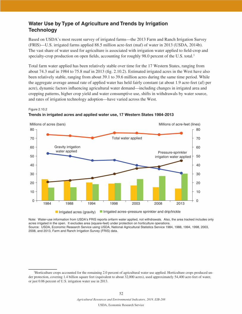
Agricultural Resources and Environmental Indicators, 2019, EIB-208
USDA, Economic Research Service
52
Water Use by Type of Agriculture and Trends by Irrigation Technology
Based on USDA’s most recent survey of irrigated farms—the 2013 Farm and Ranch Irrigation Survey (FRIS)—U.S. irrigated farms applied 88.5 million acre-feet (maf) of water in 2013 (USDA, 2014b). The vast share of water used for agriculture is associated with irrigation water applied to field-crop and specialty-crop production on open fields, accounting for roughly 98.0 percent of the U.S. total.3
Total farm water applied has been relatively stable over time for the 17 Western States, ranging from about 74.3 maf in 1984 to 75.8 maf in 2013 (fig. 2.10.2). Estimated irrigated acres in the West have also been relatively stable, ranging from about 39.1 to 39.6 million acres during the same time period. While the aggregate average annual rate of applied water has held fairly constant (at about 1.9 acre-feet (af) per acre), dynamic factors influencing agricultural water demand—including changes in irrigated area and cropping patterns, higher crop yield and water consumptive use, shifts in withdrawals by water source, and rates of irrigation technology adoption—have varied across the West.
Figure 2.10.2
Trends in irrigated acres and applied water use, 17 Western States 1984-2013
Millions of acres (bars)
0
10
20
30
40
50
60
70
80
0
10
20
30
40
50
60
70
80
1984 1988 1994 1998 2003 2008 2013
Irrigated acres (gravity) Irrigated acres–pressure sprinkler and drip/trickle
Total water applied
Gravity irrigationwater applied Pressure-sprinkler
irrigation water applied
Millions of acre-feet (lines)
Note: Water-use information from USDA’s FRIS reports onfarm water applied, not withdrawals. Also, the area tracked includes only acres irrigated in the open. It excludes area (square-feet) under protection on horticulture operations. Source: USDA, Economic Research Service using USDA, National Agricultural Statistics Service 1984, 1988, 1994, 1998, 2003, 2008, and 2013, Farm and Ranch Irrigation Survey (FRIS) data.
3Horticulture crops accounted for the remaining 2.0 percent of agricultural water use applied. Horticulture crops produced un-der protection, covering 1.4 billion square feet (equivalent to about 32,000 acres), used approximately 54,400 acre-feet of water, or just 0.06 percent of U.S. irrigation water use in 2013.
Agricultural Resources and Environmental Indicators, 2019, EIB-208
USDA, Economic Research Service
53
The shift from gravity-flow to pressurized-sprinkler application systems has been particularly significant. In general, annual applied water rates under pressurized-sprinkler systems are considerably lower than under gravity-flow systems (1.2 af/acre compared with 2.3 af/acre across the West in 2013). In 1984, 62 percent of irrigated acres relied on gravity systems, compared with just 34 percent of irrigated acres in 2013. Over the same period, the share of Western irrigated acres using pressure-sprinkler (including drip/trickle) irrigation systems rose from 37 to 76 percent (with some acres irrigated with both systems). The corresponding shift in Western applied water use by irrigation technology has been more dramatic as water scarcity has intensified. Water applied using gravity systems steadily declined from 71 percent to 41 percent of total applied water, with a corresponding increase in water applied with pressure-sprinkler systems. While the trend from gravity to sprinkler systems is observed over the entire 30-year period, the decline in gravity systems and concurrent expansion in sprinkler area and water use accelerated after the late 1990s. The extent and timing of these shifts, however, vary significantly across the Western States.
Farm-Size Characteristics of Irrigated Agriculture
Most irrigated farms are low-sales farm operations with under $150,000 in annual farm sales. Of the 229,200 irrigated farms across the United States in 2013, 64 percent were low-sales farms.4 However, large-scale farms—those with $1,000,000 or more in farm sales—occupy most of the irrigated acres and use most of the applied irrigation water. These farms account for 60 percent of U.S. irrigated area and 61.5 percent of farm water applied. For the Western States, the largest irrigated farms—those with farm sales of $350,000 or more (22 percent of irrigated farms)—account for nearly 80 percent of the region’s applied irrigation water.
Large-scale irrigated farms account for most of the value (79 percent) of farm production sales from irri-gated farms, reflecting both their larger acreages and more extensive investment in irrigation systems. Low- and moderate-sales irrigated farms, which account for 75-78 percent of all irrigated farms, accounted for just 7.7 percent of irrigated farm production sales. For all irrigated farms, the average farm sales ($ per farm) across the United States in 2012 was nearly four times that of farms not irrigating: $514,400 per irrigated farm, compared to $133,600 per nonirrigated farm.5
Importance of Conservation for Irrigated Agriculture
Many forces─such as population and economic growth, expansion of the U.S. energy sector, Native American water-right claims, and water quality and ecosystem restoration initiatives—are driving increased demands for water resources across the country. On the supply side, continued overdraft of groundwater aquifers (where withdrawals exceed annual hydrologic recharge) is expected to reduce the future availability of groundwater supplies for irrigation use in important agricultural regions. While the precise effect of climate change on water resources is uncertain, climate change is projected to shrink surface-water supplies in much of the West through reduced snowpack, shifting precipitation patterns, and higher evaporative losses. At the same time, warming temperatures are expected to contribute to
4Farm-size characteristics of irrigated farms were summarized based on USDA data from the 2013 Farm and Ranch Irriga-tion Survey (FRIS). Four farm-size classes were examined based on the “total farm sales (FS)” variable acquired from the 2012 Census of Agriculture: (1) low-sales farms (FS < $150,000); (2) moderate-sales farms (FS $150,000 to < $350,000); (3) mid-size farms (FS $350,000 to < $1,000,000); and (4) large-scale farms (FS $1,000,000 and more). See chapter 1.1, “Farm Numbers and Size,” for characteristics of all farms (irrigated plus non-irrigated).
5For more detailed information on U.S. irrigated agriculture characteristics by farm-size class, see the ERS data product “Irri-gated Agriculture in the United States.”

Agricultural Resources and Environmental Indicators, 2019, EIB-208
USDA, Economic Research Service
54
increased water demands due to rising evapotranspiration rates and potentially greater frequency and severity of drought (Georgakakos et al., 2014). In most river basins of the Western States, surface-water supplies are fully appropriated, and opportunities for large-scale water-supply development are limited. These trends, taken together, are expected to intensify competition for existing water allocations, height-ening the importance of water conservation for a sustainable irrigated agriculture sector.
Onfarm Irrigation Efficiency: Benefits and Opportunities for Improvement
Improvements in physical irrigation systems and water management have helped to increase onfarm irrigation efficiency, or the share of applied water that is beneficially used for crop production. Gains in water-use efficiency provide various farm-level benefits, including improved crop yields and potential savings in water costs and other applied inputs. Improved water-use efficiencies, particularly when imple-mented in concert with watershed-scale conservation measures that limit expansion in irrigated area or reduce water withdrawals, can provide off-farm benefits as well, including fish and wildlife habitat, and reduced ecosystem and human health risks associated with environmental degradation.
While substantial technological innovation has already occurred in U.S. irrigated agriculture, additional water-use efficiency gains are achievable (Schaible and Aillery, 2016; see also chapter 3.16, “Farm-Level Adaptation to Drought Risk”).6 Based on FRIS results, much of the growth in high-efficiency systems reflects the expansion in pressurized sprinklers and micro-irrigation systems (fig. 2.10.3). The share of acres using more efficient gravity systems peaked in the late 1990s, but then declined as farmers increasingly turned to the even more efficient pressure-sprinkler/micro-spray and drip systems. However, more than half of irrigated cropland acres in the West continue to be irrigated with more traditional application systems.
Figure 2.10.3
Trends in the shares of acres irrigated with more efficient irrigation systems, by system type, for the 17 Western States, 1994-2013
Percent
37
11
52
0
20
40
60
80
100
1994 1998 2003 2008 2013
Traditional sprinkler or gravity systems
More efficient gravity systems
More efficient pressure sprinkler systems
34
14
52
27
17
56
23
25
52
15
21
63
Note: Efficient gravity irrigation includes furrow irrigated acres using above- or below-ground pipe, or a lined open-ditch field water-delivery system, plus acres in flood irrigation (between borders or within basins) on farms using laser-leveling and pipe or lined open-ditch field water-delivery systems. Efficient pressure-sprinkler irrigation includes acres using either drip/trickle and low-flow micro systems or lower pressure-sprinkler systems [pressure per square-inch (PSI) < 30]. Traditional irrigation includes all remaining irrigated acres associated with traditional irrigation systems, including less water-use efficient gravity and sprinkler systems. Source: USDA, Economic Research Service, using data from USDA’s National Agricultural Statistics Service Farm and Ranch Irrigation Surveys (FRIS) for 1994, 1998, 2003, 2008, and 2013.
6To assess shifts in relative irrigation efficiency over time, Schaible and Aillery (2016) characterize irrigation systems as either “traditional” or “efficient” depending on acreage by irrigation application system and their components reported in the FRIS for both gravity and pressurized systems.

Agricultural Resources and Environmental Indicators, 2019, EIB-208
USDA, Economic Research Service
55
FRIS data also indicate the potential for increased irrigation efficiency through more extensive use of onfarm water-management practices that improve the rate and timing of applied water. Fewer than 10 percent of irrigators make use of soil- or plant-moisture sensing devices or commercial irrigation scheduling services, while fewer than 2 percent use computer-based crop-growth simulation models to determine irrigation requirements based on consumptive-use needs by crop-growth stage under local weather conditions.
Irrigation Investments and Continued Agricultural Water Conservation
Irrigators annually make significant capital investments in onfarm irrigation equipment and infrastruc-ture—$2.6 billion in 2013 (72 percent in the West), with the large majority (90 percent) of these invest-ments financed privately. Farms receiving public financial assistance for irrigation investments through USDA’s Environmental Quality Incentives Program (EQIP) represent fewer than 5 percent of all irrigated farms reporting irrigation investments.
Further improvements in farm water conservation remain an important USDA farm policy goal (USDA, 2018). Through improved irrigation production systems that combine investments in irrigation tech-nology with innovative water-management practices (e.g., a low-pressure sprinkler system with use of advanced sensor technologies), producers are better able to maximize the efficiency of their irrigation systems. Potential for real water savings at the watershed scale will depend on reduced system losses, the disposition of those losses (e.g., evaporation versus recharge), and as necessary, managed reductions in consumptive water use under more highly efficient systems. Institutional measures—such as tiered water pricing, withdrawal restrictions, water markets, conserved water rights, and instream flow requirements—may further incentivize investments in irrigation efficiency for farm-level water conservation or environ-mental quality protection.
References
Georgakakos, A., P. Fleming, M. Dettinger, C. Peters-Lidard, Terese (T.C.) Richmond, K. Reckhow, K. White, and D. Yates. 2014. “Water Resources,” Climate Change Impacts in the United States: The Third National Climate Assessment. J.M. Melillo, Terese (T.C.) Richmond, and G.W. Yohe, Eds. Glob-al Change Research Program. doi:10.7930/J0G44N6T.
Schaible, G.D., and M.P. Aillery. 2016. “Challenges for US Irrigated Agriculture in the Face of Emerging Demands and Climate Change,” Competition for Water Resources: Experiences and Management Ap-proaches in the US and Europe. Jadwiga Ziolkowska and Jeffrey Peterson, eds. Elsevier Publishing.
Schaible, G.D. 2017. Irrigated Agriculture in the United States. ERS Data Product. U.S. Department of Agriculture (USDA). 2014a. 2012 Census of Agriculture, National Agricultural Statis-
tics Service, Vol. 1, Part 51 (AC-12-A-51). U.S. Department of Agriculture (USDA). 2014b. Farm and Ranch Irrigation Survey, 2013, National Agri-
cultural Statistics Service, Vol. 3, Special Studies, Part 1 (AC-12-SS-1).U.S. Department of Agriculture (USDA). 2018. USDA Strategic Plan – FY 2018-2022. U.S. Department of Agriculture, Natural Resources Conservation Service (USDA-NRCS). 2017. NRCS
Conservation Programs – EQIP Financial Information (2009–16).U.S. Geological Survey (USGS). 1998. Estimated Use of Water in the United States in 1995. Circular
1200, U.S. Department of Interior, Reston, VA. U.S. Geological Survey (USGS). 2018. Estimated Use of Water in the United States in 2015. Circular
1441, U.S. Department of Interior, Reston, VA.
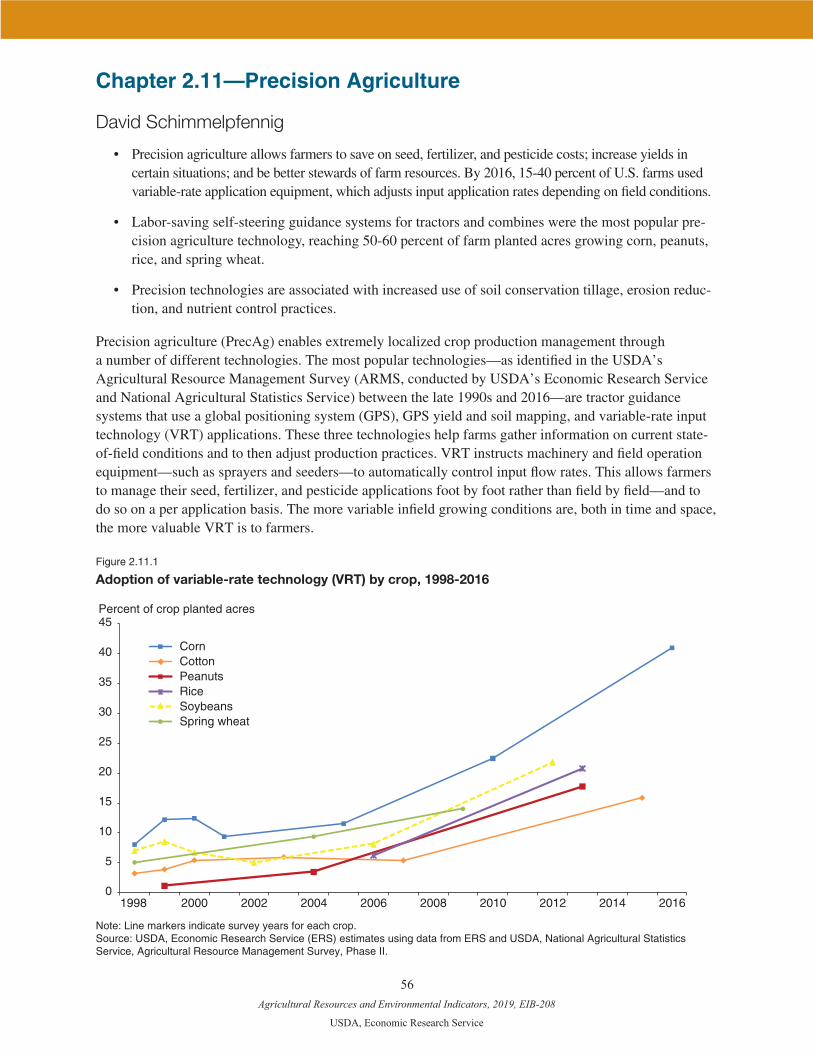
Agricultural Resources and Environmental Indicators, 2019, EIB-208
USDA, Economic Research Service
56
Chapter 2.11—Precision Agriculture
David Schimmelpfennig
• Precision agriculture allows farmers to save on seed, fertilizer, and pesticide costs; increase yields in certain situations; and be better stewards of farm resources. By 2016, 15-40 percent of U.S. farms used variable-rate application equipment, which adjusts input application rates depending on field conditions.
• Labor-saving self-steering guidance systems for tractors and combines were the most popular pre-cision agriculture technology, reaching 50-60 percent of farm planted acres growing corn, peanuts, rice, and spring wheat.
• Precision technologies are associated with increased use of soil conservation tillage, erosion reduc-tion, and nutrient control practices.
Precision agriculture (PrecAg) enables extremely localized crop production management through a number of different technologies. The most popular technologies—as identified in the USDA’s Agricultural Resource Management Survey (ARMS, conducted by USDA’s Economic Research Service and National Agricultural Statistics Service) between the late 1990s and 2016—are tractor guidance systems that use a global positioning system (GPS), GPS yield and soil mapping, and variable-rate input technology (VRT) applications. These three technologies help farms gather information on current state-of-field conditions and to then adjust production practices. VRT instructs machinery and field operation equipment—such as sprayers and seeders—to automatically control input flow rates. This allows farmers to manage their seed, fertilizer, and pesticide applications foot by foot rather than field by field—and to do so on a per application basis. The more variable infield growing conditions are, both in time and space, the more valuable VRT is to farmers.
Figure 2.11.1
Adoption of variable-rate technology (VRT) by crop, 1998-2016
Percent of crop planted acres
0
5
10
15
20
25
30
35
40
45
1998 2000 2002 2004 2006 2008 2010 2012 2014 2016
CornCottonPeanutsRiceSoybeansSpring wheat
Note: Line markers indicate survey years for each crop.Source: USDA, Economic Research Service (ERS) estimates using data from ERS and USDA, National Agricultural Statistics Service, Agricultural Resource Management Survey, Phase II.
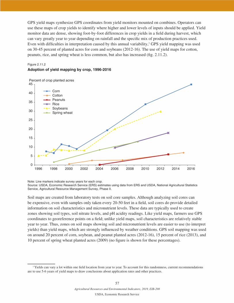
Agricultural Resources and Environmental Indicators, 2019, EIB-208
USDA, Economic Research Service
57
GPS yield maps synthesize GPS coordinates from yield monitors mounted on combines. Operators can use these maps of crop yields to identify where higher and lower levels of inputs should be applied. Yield monitor data are dense, showing foot-by-foot differences in crop yields in a field during harvest, which can vary greatly year to year depending on rainfall and the specific mix of production practices used. Even with difficulties in interpretation caused by this annual variability,1 GPS yield mapping was used on 30-45 percent of planted acres for corn and soybeans (2012-16). The use of yield maps for cotton, peanuts, rice, and spring wheat is less common, but also has increased (fig. 2.11.2).
Figure 2.11.2
Adoption of yield mapping by crop, 1996-2016
Percent of crop planted acres
0
5
10
15
20
25
30
35
40
45
1996 1998 2000 2002 2004 2006 2008 2010 2012 2014 2016
CornCottonPeanutsRiceSoybeansSpring wheat
Note: Line markers indicate survey years for each crop.Source: USDA, Economic Research Service (ERS) estimates using data from ERS and USDA, National Agricultural Statistics Service, Agricultural Resource Management Survey, Phase II.
Soil maps are created from laboratory tests on soil core samples. Although analyzing soil cores can be expensive, even with samples only taken every 20-50 feet in a field, soil cores do provide detailed information on soil characteristics and micronutrient levels. These data are typically used to create zones showing soil types, soil nitrate levels, and pH acidity readings. Like yield maps, farmers use GPS coordinates to georeference points on a field; unlike yield maps, soil characteristics are relatively stable year to year. Thus, zones on soil maps showing soil and micronutrient levels are easier to use (to interpret yields) than yield maps, which are strongly influenced by weather conditions. GPS soil mapping was used on around 20 percent of corn, soybean, and peanut planted acres (2012-16), 15 percent of rice (2013), and 10 percent of spring wheat planted acres (2009) (no figure is shown for these percentages).
1 Yields can vary a lot within one field location from year to year. To account for this randomness, current recommendations are to use 5-6 years of yield maps to draw conclusions about application rates and other practices.
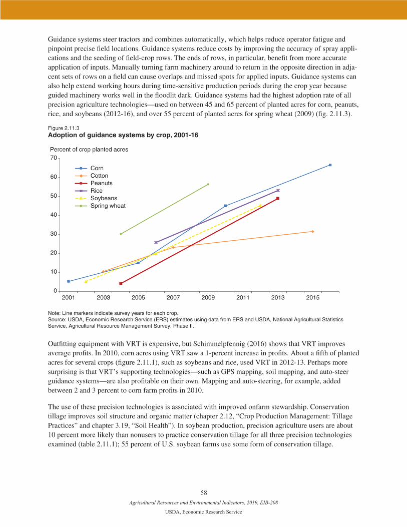
Agricultural Resources and Environmental Indicators, 2019, EIB-208
USDA, Economic Research Service
58
Guidance systems steer tractors and combines automatically, which helps reduce operator fatigue and pinpoint precise field locations. Guidance systems reduce costs by improving the accuracy of spray appli-cations and the seeding of field-crop rows. The ends of rows, in particular, benefit from more accurate application of inputs. Manually turning farm machinery around to return in the opposite direction in adja-cent sets of rows on a field can cause overlaps and missed spots for applied inputs. Guidance systems can also help extend working hours during time-sensitive production periods during the crop year because guided machinery works well in the floodlit dark. Guidance systems had the highest adoption rate of all precision agriculture technologies—used on between 45 and 65 percent of planted acres for corn, peanuts, rice, and soybeans (2012-16), and over 55 percent of planted acres for spring wheat (2009) (fig. 2.11.3).
Figure 2.11.3 Adoption of guidance systems by crop, 2001-16
Percent of crop planted acres
CornCottonPeanutsRiceSoybeansSpring wheat
0
10
20
30
40
50
60
70
2001 2003 2005 2007 2009 2011 2013 2015
Note: Line markers indicate survey years for each crop.Source: USDA, Economic Research Service (ERS) estimates using data from ERS and USDA, National Agricultural Statistics Service, Agricultural Resource Management Survey, Phase II.
Outfitting equipment with VRT is expensive, but Schimmelpfennig (2016) shows that VRT improves average profits. In 2010, corn acres using VRT saw a 1-percent increase in profits. About a fifth of planted acres for several crops (figure 2.11.1), such as soybeans and rice, used VRT in 2012-13. Perhaps more surprising is that VRT’s supporting technologies—such as GPS mapping, soil mapping, and auto-steer guidance systems—are also profitable on their own. Mapping and auto-steering, for example, added between 2 and 3 percent to corn farm profits in 2010.
The use of these precision technologies is associated with improved onfarm stewardship. Conservation tillage improves soil structure and organic matter (chapter 2.12, “Crop Production Management: Tillage Practices” and chapter 3.19, “Soil Health”). In soybean production, precision agriculture users are about 10 percent more likely than nonusers to practice conservation tillage for all three precision technologies examined (table 2.11.1); 55 percent of U.S. soybean farms use some form of conservation tillage.

Agricultural Resources and Environmental Indicators, 2019, EIB-208
USDA, Economic Research Service
59
Erosion control refers to structures erected for grade stabilization, as well as water-control basins, filter strips, field borders, and contour farming/strip cropping. These practices are used on about one-third of all soybean farms, with 5-8 percent more precision agriculture users than nonusers practicing erosion control; guidance users are the most likely to practice erosion control (relative to nonusers of guidance).
Fertilizer is applied to benefit production, but when fertilizer is overapplied it can degrade water resources through runoff and groundwater contamination. Farmers indicated in their ARMS survey responses if they had changed any of their cropping practices to reduce their use of fertilizer or applied nutrients on soybean fields (2012) (most commonly potassium, phosphorus, or lime, as soybeans are nitrogen-fixing) or changed the type of fertilizer used on rice paddies (2013) to reduce fertilizer use. Almost one-quarter of both soybean and rice farmers indicated that they had changed practices to reduce fertilizer use, and a statistically higher number of these farmers used precision agriculture than did not (table 2.11.1).
Variable-rate technology (VRT) provides interesting crop comparisons. When VRT was adopted on soybean farms, the share of farms that reduced fertilizer use increased by 17 percent (from 21 to 38 percent). This suggests that soybean farmers use VRT as a way to reduce fertilizer use. For rice farms that reduced fertilizer, on the other hand, the difference between the share of VRT users and nonusers is only 2 percent. Overall, VRT use in rice has climbed to over 20 percent, suggesting that many rice farmers use VRT to increase the accuracy of fertilizer placement without reducing their overall use of fertilizer. This means that VRT may not help reduce fertilizer use in all cases but, in some circumstances, fertilizer savings with VRT can be substantial.2
Table 2.11.1
Best management practices on soybeans and rice, by precision agriculture technology, 2012-13
Percent of farms using practice, by precision technology
Crop and practicePercent of all farms
GPS soil/Yieldmapping
Guidancesystem
Variable-rate technology
Yes No Yes No Yes No
Soybeans (2012): soil care
Conservation tillage 55 61* 53 63** 51 62** 53
Erosion control 36 40* 34 41* 33 40* 35
Reduced fertilizer use
Rice (2013) 23 28** 22 27** 19 25 23
Soybeans (2012) 24 31* 22 29* 22 38** 21
Note: Asterisks reflect 98- and 90-percent confidence (** and *, respectively) in a significant difference between precision technology adopters (Yes) and nonadopters (No) in the use of conservation tillage, erosion control practices, and reduced fertilizer. GPS = Global Positioning System.Source: USDA Economic Research Service (ERS) estimates using data from ERS and USDA, National Agricultural Statistics Service, Agricultural Resource Management Survey, Phase II.
2While other chemicals can be applied using the VRT method, fertilizer is typically the most important from a cost and yield impact perspective. Rice is an exception, where nonfertilizer chemicals applications using VRT have bigger payoffs.
Agricultural Resources and Environmental Indicators, 2019, EIB-208
USDA, Economic Research Service
60
Several factors are likely to influence the effectiveness of precision technologies in the future. Wireless sensor technologies for crop plants or soil are likely to increase the volume of data on growing conditions available to farmers. Internet-enabled devices can collect sensor data and make crop practice recommen-dations in real time in a farmer’s fields. These developing technologies are likely to be combined with programming known as artificial intelligence (AI), or application equipment may be built with machine-learning capability that can supply more sophisticated recommendations to farmers. These AI and machine-learning innovations can combine data that are growing more plentiful in new ways to produce novel insights on crop-practice effectiveness. This evolution of data availability and data use is going on while farmers are developing more data-driven relationships with trusted advisors and agricultural input retailers, who may use these data resources to help farmers come closer to fully exploiting their data.
References
Schimmelpfennig, D. 2016. Farm Profits and Adoption of Precision Agriculture. ERR-217, U.S. Department of Agriculture, Economic Research Service.

Agricultural Resources and Environmental Indicators, 2019, EIB-208
USDA, Economic Research Service
61
Chapter 2.12—Crop Production Management: Tillage Practices
Tara Wade and Roger Claassen
• Conservation tillage is used widely on major crops, including 70 percent of soybeans (2012), 40 percent of cotton (2015), 65 percent of corn (2016), and 67 percent of wheat (2017).
• No-till (a form of conservation tillage) varies widely across crops, including 40 percent of soybeans (2012), 18 percent of cotton (2015), 27 percent of corn (2016), and 45 percent of wheat (2017).
• Farms that alternate no-till/strip-till with full-width tillage include roughly 30 percent of all corn, soybean, cotton, and wheat acreage
Reducing or eliminating tillage can reduce soil erosion, conserve soil moisture, and promote better soil health by minimizing soil disturbance and keeping crop residues on the soil surface (Bowman et al., 2016; see also chapter 3.19, “Soil Health” ). Conservation tillage encompasses a range of tillage practices. In a no-till system, farmers plant directly into the undisturbed soil with the residue of the previous crop still on the soil surface. In a mulch-till system, the soil is tilled lightly but much of the previous crop residue is maintained on the soil surface. In a strip-till system soil disturbance is limited by tilling only narrow strips where seeds are planted, also providing an opportunity to place fertilizer below the soil surface.
No-till is more efficient than mulch-till in terms of soil health, soil moisture conservation, and soil erosion control because it causes less soil disturbance and maintains greater soil residue cover. When compared to mulch-till, no-till can also mitigate sediment and nutrient loading in bodies of water and preserve soil depth and productivity (Rittenburg et al., 2015). Limiting soil disturbance and maintaining residue can also increase soil carbon sequestration and improve soil properties in a number of ways, including increased water holding capacity, higher soil organic matter content, and reduced soil compac-tion (USDA, NRCS, 1996). Evidence also suggests, however, that long-term gains in soil health can be achieved only through consistent application of a suite of practices that includes minimal tillage and practices that increase (1) residue cover and (2) the portion of the year soil is covered by a growing crop (using cover crops, for example) (USDA, NRCS, 2014).
Conservation practices are often part of conservation plans required for highly erodible cropland to main-tain eligibility for most Federal agricultural programs. Climate and weather may also play a role in the tillage decision; farmers may use no-till or strip-till to conserve soil moisture in dryer regions or when soil moisture reserves are low, but use other tillage systems when soil moisture is ample (Ding et al., 2009) or in relatively cold conditions (Soule et al., 2000).
Tillage Practices Vary by Crop
In the field-level portion of USDA’s Agricultural Resource Management Survey (ARMS), producers of specific crops are surveyed on a multiyear cycle (e.g., corn producers were surveyed in 2005, 2010, and 2016) to generate a wide range of information on crop production practices. Tillage estimates are based on the sequence of field operations as reported by respondents. Tillage practices can be defined by
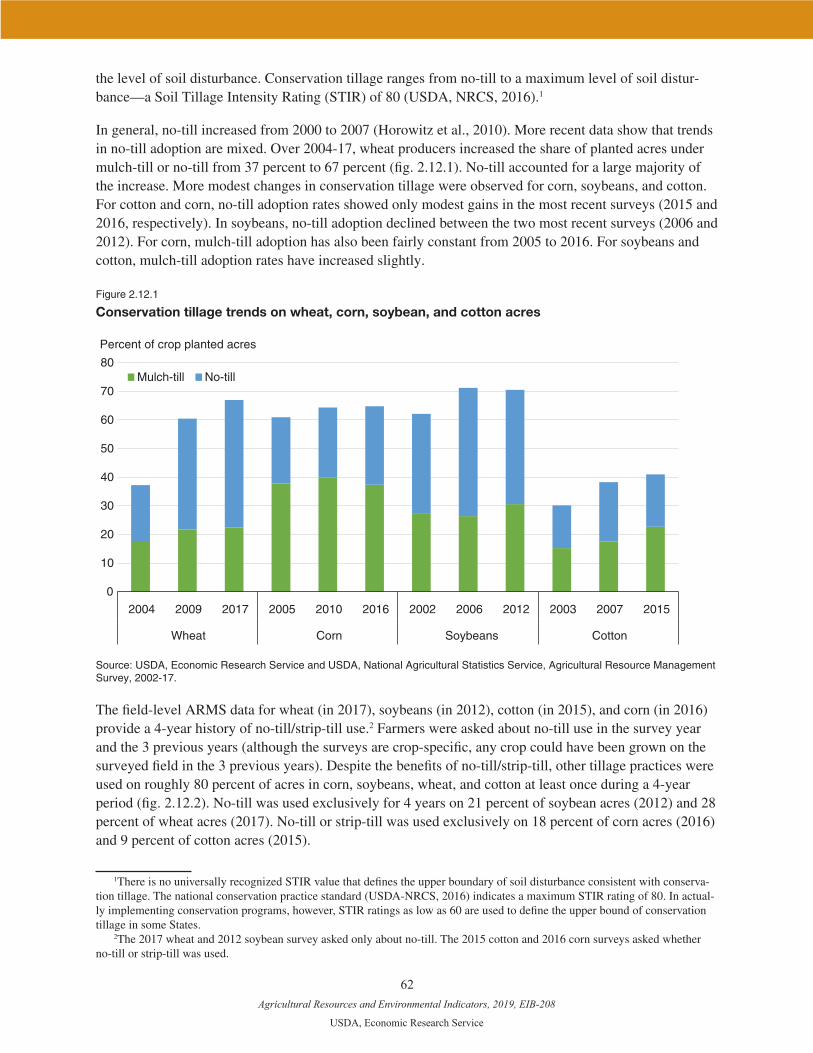
Agricultural Resources and Environmental Indicators, 2019, EIB-208
USDA, Economic Research Service
62
the level of soil disturbance. Conservation tillage ranges from no-till to a maximum level of soil distur-bance—a Soil Tillage Intensity Rating (STIR) of 80 (USDA, NRCS, 2016).1
In general, no-till increased from 2000 to 2007 (Horowitz et al., 2010). More recent data show that trends in no-till adoption are mixed. Over 2004-17, wheat producers increased the share of planted acres under mulch-till or no-till from 37 percent to 67 percent (fig. 2.12.1). No-till accounted for a large majority of the increase. More modest changes in conservation tillage were observed for corn, soybeans, and cotton. For cotton and corn, no-till adoption rates showed only modest gains in the most recent surveys (2015 and 2016, respectively). In soybeans, no-till adoption declined between the two most recent surveys (2006 and 2012). For corn, mulch-till adoption has also been fairly constant from 2005 to 2016. For soybeans and cotton, mulch-till adoption rates have increased slightly.
Figure 2.12.1
Conservation tillage trends on wheat, corn, soybean, and cotton acres
Percent of crop planted acres
0
10
20
30
40
50
60
70
80
2004 2009 2017 2005 2010 2016 2002 2006 2012 2003 2007 2015
Wheat Corn Soybeans Cotton
Mulch-till No-till
Source: USDA, Economic Research Service and USDA, National Agricultural Statistics Service, Agricultural Resource Management Survey, 2002-17.
The field-level ARMS data for wheat (in 2017), soybeans (in 2012), cotton (in 2015), and corn (in 2016) provide a 4-year history of no-till/strip-till use.2 Farmers were asked about no-till use in the survey year and the 3 previous years (although the surveys are crop-specific, any crop could have been grown on the surveyed field in the 3 previous years). Despite the benefits of no-till/strip-till, other tillage practices were used on roughly 80 percent of acres in corn, soybeans, wheat, and cotton at least once during a 4-year period (fig. 2.12.2). No-till was used exclusively for 4 years on 21 percent of soybean acres (2012) and 28 percent of wheat acres (2017). No-till or strip-till was used exclusively on 18 percent of corn acres (2016) and 9 percent of cotton acres (2015).
1There is no universally recognized STIR value that defines the upper boundary of soil disturbance consistent with conserva-tion tillage. The national conservation practice standard (USDA-NRCS, 2016) indicates a maximum STIR rating of 80. In actual-ly implementing conservation programs, however, STIR ratings as low as 60 are used to define the upper bound of conservation tillage in some States.
2The 2017 wheat and 2012 soybean survey asked only about no-till. The 2015 cotton and 2016 corn surveys asked whether no-till or strip-till was used.

Agricultural Resources and Environmental Indicators, 2019, EIB-208
USDA, Economic Research Service
63
Figure 2.12.2
Half of fields are tilled each year, 2012-2017
0
10
20
30
40
50
60
70
Corn,2016
Cotton,2015
Soybeans,2012
Wheat,2017
Percent of planted acres
Continuous full-width tillage
Alternating full-width tillage w/no-till/strip-till
Continuous no-till or strip-till
4930
21
Corn, cotton, soybeans, and wheat combined
Note: “No-till” means planting without tilling since the previous harvest. “Strip-till” means tilling only a narrow strip over the row (used only in row crops). “Full-width” tillage is tilling the entire soil surface. For each survey, respondents are asked whether no-till or strip-till was used in each year over a 4-year period. For example, “continuous” no-till or strip-till means that no-till or strip-till was used in each year of the 4-year period. Source: USDA, Economic Research Service and USDA, National Agricultural Statistics Service, Agricultural Resource Management Survey, 2012, 2015, 2016, and 2017.
Many Farmers Use No-Till or Strip-Till on a Portion of Their Cropland
Many farmers who use no-till use it on only a portion of their crop acreage. For example, farmers often rotate tillage practices along with crops (Robertson et al., 2014), using no-till/strip-till on crops that are thought to be well suited for the practices (e.g., soybeans) and conventional or mulch tillage for crops where no-till/strip-till are perceived to be more risky (e.g., corn) (Reimer et al., 2012). Some farmers may also select their tillage practice based on field characteristics. For example, farmers may use no-till/strip-till on highly erodible land to control soil erosion and use conventional tillage on land that is not highly erodible (Prokopy et al., 2008).
ARMS data for 2010-11 provide a detailed, farmwide look at how farmers used no-till/strip-till on the four most widely grown crops. During those years, 56 percent of all land used for corn, soybeans, wheat, and cotton was on farms that used no-till/strip-till on some portion of land used for these crops. Roughly 23 percent of land in these crops were on a farm where no-till/ strip-till was used on every acre (full adopters). Another 33 percent of acreage was on farms where a mix of no-till, strip-till, and other tillage practices were used (partial adopters). Partial adopters used no-till/strip-till on roughly half of their crop-land (15 percent of land in the four major crops).
Intensity of use among partial adopters varies regionally (fig. 2.12.3). Partial adopters in the Heartland, Prairie Gateway, Eastern Uplands, and Southern Seaboard used no-till/strip-till on 16-20 percent of acres in 2010-11. In the Northern Great Plains, Heartland, and Prairie Gateway regions—which account for 72 percent of U.S. corn, soybean, wheat, and cotton acreage—more than half of these crop acres were on
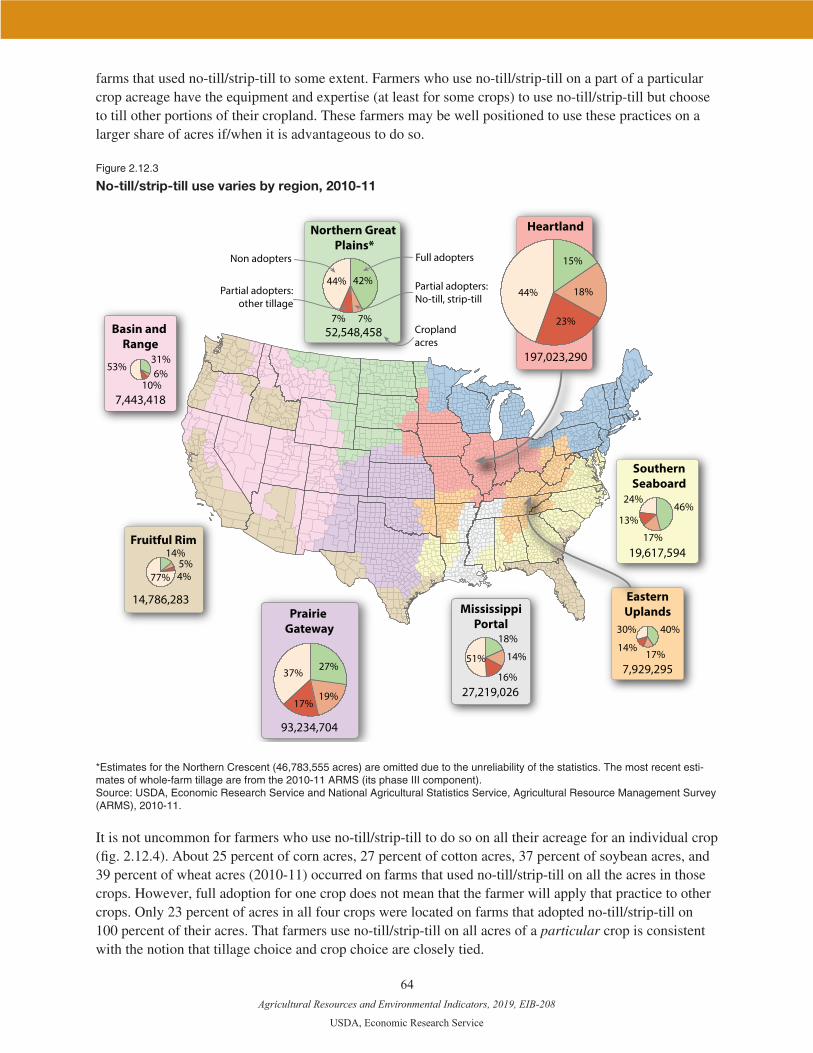
Agricultural Resources and Environmental Indicators, 2019, EIB-208
USDA, Economic Research Service
64
farms that used no-till/strip-till to some extent. Farmers who use no-till/strip-till on a part of a particular crop acreage have the equipment and expertise (at least for some crops) to use no-till/strip-till but choose to till other portions of their cropland. These farmers may be well positioned to use these practices on a larger share of acres if/when it is advantageous to do so.
Figure 2.12.3
No-till/strip-till use varies by region, 2010-11
17%
40%
14%
30%
14%
18%
16%
51%
19%
27%
17%
37%
5%14%
4%77%
6%31%
10%
53%
7%
42%
7%
44%18%
15%
23%
44%
17%
46%13%
24%
Basin and Range
7,443,418
EasternUplands
7,929,295
Fruitful Rim
14,786,283
19,617,594
SouthernSeaboard
Northern Great Plains*
52,548,458 Croplandacres
Partial adopters:other tillage
Full adopters
Partial adopters:No-till, strip-till
Prairie Gateway
MississippiPortal
27,219,026
Heartland
197,023,290
93,234,704
Non adopters
*Estimates for the Northern Crescent (46,783,555 acres) are omitted due to the unreliability of the statistics. The most recent esti-mates of whole-farm tillage are from the 2010-11 ARMS (its phase III component).Source: USDA, Economic Research Service and National Agricultural Statistics Service, Agricultural Resource Management Survey (ARMS), 2010-11.
It is not uncommon for farmers who use no-till/strip-till to do so on all their acreage for an individual crop (fig. 2.12.4). About 25 percent of corn acres, 27 percent of cotton acres, 37 percent of soybean acres, and 39 percent of wheat acres (2010-11) occurred on farms that used no-till/strip-till on all the acres in those crops. However, full adoption for one crop does not mean that the farmer will apply that practice to other crops. Only 23 percent of acres in all four crops were located on farms that adopted no-till/strip-till on 100 percent of their acres. That farmers use no-till/strip-till on all acres of a particular crop is consistent with the notion that tillage choice and crop choice are closely tied.

Agricultural Resources and Environmental Indicators, 2019, EIB-208
USDA, Economic Research Service
65
Figure 2.12.4
Farmers adopt no-till/strip-till on part of their farms, 2010-111
0
10
20
30
40
50
60
Corn Soybeans Wheat Cotton
Other tillage practices: no-till/strip-till adopted onsome crop acres
No-till/strip-till: no-till/strip-till adopted on some crop acres
No-till/strip-till: no-till/strip-till adopted on all of crop acres
Percent of acres
1The fourth category (not shown) is other tillage practices on nonadopter farms. The most recent estimates of whole-farm tillage are from the 2010-11 ARMS (its phase III component).Source: USDA, Economic Research Service and National Agricultural Statistics Service, Agricultural Resource Management Survey, 2010-11.
References
Bowman, M., S. Wallander, S., and L. Lynch. 2016. “An Economic Perspective on Soil Health,” Amber Waves, September, 2016.
Conservation Tillage Information Center. 2018. Definitions: Tillage Types. Ding, Y., K. Schoengold, and T. Tadesse. 2009. “The Impact of Weather Extremes on Agricultural Produc-
tion Methods: Does Drought Increase Adoption of Conservation Tillage Practices?” Journal of Agri-cultural and Resource Economics 34(3): 395-411.
Horowitz, J., R. Ebel, and K. Ueda. 2010. “No-Till” Farming Is a Growing Practice. EIB-70. U.S. De-partment of Agriculture, Economic Research Service.
Prokopy, L.S., K. Floress, D. Klotthor-Weinkauf, and A. Baumgart-Getz. 2008. “Determinants of Agricul-tural Best Management Practice Adoption: Evidence from the Literature,” Journal of Soil and Water Conservation 63(5): 300-11.
Reimer, A.P., D.K. Weinkauf, and L.S. Prokopy. 2012. “The Influence of Perceptions of Practice Charac-teristics: An Examination of Agricultural Best Management Practice Adoption in Two Indiana Water-sheds,” Journal of Rural Studies 28(1): 118-128.
Rittenburg, R.A., A.L. Squires, J. Boll, E.S. Brooks, Z.M. Easton, and T.S. Steenhuis. 2015. “Agricultur-al BMP effectiveness and dominant hydrological flow paths: concepts and a review,” Journal of the American Water Resources Association 51 (2): 305-329.
Robertson, G.P., K.L. Gross, S.K. Hamilton, D.A. Landis, T.M. Schmidt, S.S. Snapp, and S.M. Swinton. 2014. “Farming for Ecosystem Services: An Ecological Approach to Production Agriculture,” BioSci-ence 64(5): 404-15.
Agricultural Resources and Environmental Indicators, 2019, EIB-208
USDA, Economic Research Service
66
Soule, M., A. Tegene, and K. Wiebe. 2000. “Land tenure and the adoption of conservation practices,” American Journal of Agricultural Economics 82(4): 993-1005.
U.S. Department of Agriculture, Natural Resources Conservation Service.1996. Cover and Green Manure Crop Benefits to Soil Quality. Auburn, AL: Soil Quality Institute, Technical Note No. 1.
U.S. Department of Agriculture, Natural Resources Conservation Service (USDA-NRCS). 2014. “Soil Health Literature Summary—Effects of Conservation Practices on Soil Properties on Areas of Crop-land data product.”
U.S. Department of Agriculture, Natural Resources Conservation Service. 2016. “Conservation Practice Standard Code 345: Residue and tillage management, reduced tillage.”
Weil, R.R., and F. Magdoff. 2004. “Significance of soil organic matter to soil quality and health,” Soil Or-ganic Matter in Sustainable Agriculture. F. Magdoff, and R.R. Weil, editors. CRC Press, Boca Raton, FL.
Agricultural Resources and Environmental Indicators, 2019, EIB-208
USDA, Economic Research Service
67
Chapter 2.13—U.S. Organic Farming Systems
Catherine Greene, Claudia Hitaj, and William McBride
• The number of certified organic operations in the United States has more than doubled between 2006 and 2016 in response to rising consumer demand. U.S. organic retail sales are estimated to have reached $49 billion in 2017.
• In 2015, the most recent year with comprehensive USDA estimates, organic farming systems were used on nearly 10 percent of U.S. acres for vegetables, but were used on under 0.3 percent of U.S. corn and soybean acreage.
• Many of the practices associated with soil health—including longer crop rotations, nonchemical pest management, and cover crops—are much more widely used in organic farming systems than in conventional systems.
The long history and comprehensive standards associated with the organic food label, along with its widespread use worldwide, distinguishes organic labels from other eco-labels that have emerged in recent years. In 2000, USDA published national organic standards that reflected decades of private-sector devel-opment. USDA’s national regulatory program is designed to facilitate interstate trade, reduce fraudulent product claims, and provide consumer assurance that all organic products sold in the United States meet a high national standard. All growers, processors, and distributors that want to label or advertise their prod-ucts as organic must meet the national standard and must also be certified by a USDA-accredited State or private group unless their annual organic sales are under $5,000.
USDA regulations define organic farming as an ecological production system that fosters resource cycling, promotes ecological balance, and conserves biodiversity. Organic farmers are required to avoid most synthetic chemicals and must adopt practices that maintain or improve soil conditions and minimize erosion. Organic production systems can be used to increase farm income, as well as reduce pesticide residues in water and food, reduce nutrient pollution, improve soil tilth and organic matter, lower energy use, reduce greenhouse emissions, and enhance biodiversity (Reganold and Wachter, 2016; Delate, 2015; Baranski et al., 2014).
Consumer Demand Drives Adoption of Organic Systems
Organic products have shifted from a lifestyle choice for a small segment of consumers to a commonplace interest for many consumers. In 2014, Gallup included questions on organics in its annual food consump-tion survey for the first time and found that 45 percent of Americans actively tried to include organic foods in their diets, with an even higher share of younger survey respondents (ages 18 to 29) reporting that they actively try to include organic foods. The share of Americans with annual household income under $30,000 that actively tried to include organic foods was 42 percent, similar to the share for households with incomes of $30,000 to $74,999 (45 percent) and households with incomes over $75,000 (49 percent).
Organic retail sales have shown double-digit growth during most years since USDA set national organic standards and continue to grow rapidly. The Organic Trade Association estimated U.S. organic retail sales at $49.4 billion in 2017, up 6.4 percent from the previous year. While organically grown fresh produce is still the top organic category in terms of U.S. retail sales, U.S. organic milk products have higher price premiums and market share. According to a recent ERS analysis, the highest organic market share in 2014

Agricultural Resources and Environmental Indicators, 2019, EIB-208
USDA, Economic Research Service
68
was for organic milk (14 percent of total sales), followed by organic eggs and organic vegetables (both at nearly 7 percent), and organic fruit (nearly 6 percent) (Greene et al., 2017).
In 2015, the United States had 3.2 million acres of certified organic cropland and 2.2 million acres of certified organic pasture (including rangeland). While that land accounted for less than 1 percent of all U.S. farmland, the organic adoption rates varied widely across crop and livestock sectors. For example, organic farming systems were used on nearly 10 percent of U.S. vegetable acres in 2015, but less than 0.3 percent of acres devoted to major U.S. feed grains (corn and soybeans); the share of U.S. dairy and poultry production managed under organic systems falls in between.
The number of certified organic operations in the United States has more than doubled over the last decade in response to rising consumer demand. The United States had over 21,700 certified organic operations in 2015—60 percent were crop and livestock farmers, while 40 percent were processors, manufacturers, and other food handling operators. USDA’s organic regulatory program data show that organic farm production and food-handling operations are concentrated in California (the country’s top fruit and vegetable producer), the Northeast (which has many small-scale organic farms), and the Upper Midwest (a major producer of organic milk) (fig. 2.13.1). Northeastern States have the highest share of certified organic farmers, partic-ularly Vermont and Maine, where 5 and 6 percent, respectively, of all farmers are certified organic. In California, more than 3.6 percent of all farmers are certified organic (Greene et al., 2017).
Figure 2.13.1
Certified organic operations are concentrated in the West, Northeast, and Upper Midwest
Top 10 States in organic farm sales, 2016
Crops and livestock
Crops only
Food handlers only
Operation type
Organic sales in 2016 (million dollars)
California 2,889Pennsylvania 660Washington 636Oregon 351Texas 298Wisconsin 256New York 216Michigan 201Colorado 181North Carolina 145
Note: The category “Food handlers only” includes food processors, manufacturers, and other handlers.Source: USDA, Economic Research Service using data from USDA’s National Organic Program, Organic Integrity Database (U.S. certified operations in January 2016), and USDA’s National Agricultural Statistics Service, 2016 Certified Organic Survey.

Agricultural Resources and Environmental Indicators, 2019, EIB-208
USDA, Economic Research Service
69
Common Organic Practices Include Complex Rotations, Cover Crops, and Pasture
The ecological approach to farming defined by USDA in the national organic standards affects the entire production system (USDA-AMS, 2000). Farmers who shift to organic farming systems from more chemi-cal-intensive systems must make changes across the spectrum of their production inputs and practices.
Under organic farming systems, the fundamental components and natural processes of ecosystems—such as soil organism activities, nutrient cycling, and species distribution/competition—are used as farm management tools. Organic producers rely on complex rotations, cover crops, biological pest manage-ment, and other nonchemical practices. For example, crops are rotated, food and shelter are provided for the predators and parasites of crop pests, crop residues are cycled, and planting/harvesting dates are care-fully timed (USDA-NRCS, 2016). Conventional farmers use these practices much less frequently than organic farmers.
Since the mid-2000s, USDA has surveyed specific organic commodity sectors in the detailed Agricultural Resource Management Survey (ARMS), and also has begun conducting periodic surveys of all organic producers. ERS studies based on data from these surveys confirm that many of the practices associated with soil health are much more widely used in organic farming systems than in conventional systems (see chapter 3.19, “Soil Health”). For example, organic soybean producers often rotate row crops with small grain and meadow crops, and include an idle year in the rotation, while conventional producers mainly use a rotation of continuous row crops (McBride and Greene, 2009). Almost all conventional soybean producers use chemical pesticides for pest and weed control, while organic producers rely on a suite of nonchemical practices. ERS studies show similar patterns for the other field crops.
Other practices that contribute to soil health, soil productivity, and nutrient cycling—including cover crops, animal manure, and compost—are also more widely used in organic farming systems. Data from USDA’s national surveys show that nearly 40 percent of all organic field crop and specialty crop producers use cover crops, much higher than among conventional producers (fig. 2.13.2). According to ARMS data, over half of organic apple producers and over 20 percent of organic corn producers use compost, compared with under 3 percent of conventional apple and corn producers (Osteen et al., 2012). Animal manure is also much more widely used in organic field crop production than conventional production.
Tillage is more widely used in organic systems than in conventional systems, and no-till organic systems are still not used commercially in most parts of the country. In a no-till system, farmers plant directly into the undisturbed residue of the previous crop without tillage, except for nutrient injection, which can reduce soil erosion and sediment loss to water and wind. It can also increase soil carbon sequestration (the amount of carbon retained in the soil) and improve the physical, chemical, and biological properties of the soil. Organic no-till systems generally require specialized farm equipment to drill seed into cover crop residues and are more challenging to implement than conventional no-till systems, which rely on chemical herbicides to kill vegetation. Despite heavier use of tillage in organic farming, long-term crop-ping system experiments at Iowa State University, USDA-Beltsville, Rodale Institute, the University of Minnesota, and others have found that organic cropping systems can sequester as much soil organic carbon, for example, as no-till conventional systems (Delate, 2015).

Agricultural Resources and Environmental Indicators, 2019, EIB-208
USDA, Economic Research Service
70
Figure 2.13.2
Cover crops and rotational grazing are more widely used by organic producers, 2012-14
Percent of farms using practice
0
10
20
30
40
50
60
70
Cover crop (field cropproducers)
Cover crop (specialty cropsproducers)
Rotational grazing (livestockproducers)
Organic Non-organic
Source: USDA, Economic Research Service using data from 2012 Census of Agriculture (conventional producers) and the 2014 National Organic Producer Survey (certified organic producers).
Organic livestock production systems attempt to accommodate an animal’s natural nutritional and behav-ioral requirements and prohibit the use of antibiotics and hormones in livestock production. USDA organic regulations require that organic dairy cows and other ruminant livestock obtain part of their dry matter intake (forage) from pasture during the grazing season, while many conventional dairy operations did not use any forage from pasture as part of their feeding mix (McBride and Greene, 2009). Rotational grazing—managing where and when livestock graze in order to prevent overgrazing and to optimize pasture growth—is a soil health strategy that is also used more frequently in the organic dairy sector. According to USDA’s 2012 Census of Agriculture, 65 percent of organic livestock producers use rota-tional grazing, compared with 22 percent of conventional livestock producers (fig. 2.13.2).
USDA Has Expanded Conservation Assistance to Organic Producers
USDA requires a 3-year transition period before conventional farmers can earn organic price premiums, and organic producers also face many challenges after transitioning. Respondents to USDA’s ARMS organic surveys have indicated that weed control, certification paperwork, compliance costs, and input sourcing are among the most difficult aspects of organic production (McBride et al., 2015; McBride and Greene, 2009). Also, U.S. organic producers who grow crops near genetically engineered (GE) crop operations use avoidance practices, such as delaying corn planting until after GE corn is planted, to mini-mize accidental mixing of organic and GE crops (fig. 2.13.3), which may lower yields from planting at a suboptimal time (Greene et al., 2016).

Agricultural Resources and Environmental Indicators, 2019, EIB-208
USDA, Economic Research Service
71
Figure 2.13.3
Certified organic corn was planted later than genetically engineered (GE) corn in 2010 to avoid cross-pollination
0 10 20 30 40 50 60
Wisconsin ***
South Dakota ***
Ohio ***
Nebraska ***
Missouri ***
Minnesota ***
Michigan ***
Kansas **
Iowa ***
Indiana ***
Illinois ***
Mean planting date (relative to April 1)
Organic planting date GE planting date
Note: Asterisks denote a statistically significant difference between the GE and organic planting date means at the 5-percent (**) and 1-percent (***) levels.Source: USDA, Economic Research Service using data from USDA’s 2010 Agricultural Resource Management Survey Corn Survey.
Since the early 2000s, USDA and Congress have widened access for organic and transitioning producers to conservation, risk management, and other farm programs. The 2008 Farm Act, for example, expanded USDA’s Environmental Quality Incentives Program (EQIP) to include conservation practices related to organic production, as well as those related to conventional production. Congress designated lower payment caps for the EQIP Organic Initiative than for the regular EQIP program, although organic and transitioning farmers compete against a smaller pool of applicants and can also choose to enroll in the regular program instead. Under the Organic EQIP Initiative, USDA provided more than 6,800 farms across the country with $115 million in assistance between 2009 and 2016 to help producers implement conservation practices on organic and transitioning farms (fig 2.13.4). This program may be particularly useful for transitioning farmers who have not already adopted many of the conservation practices used in organic production.

Agricultural Resources and Environmental Indicators, 2019, EIB-208
USDA, Economic Research Service
72
Figure 2.13.4
Environmental Quality Incentives Program (EQIP) funding for organic and transition practices, 2009-2016
$0 $4,000,000 $8,000,000 $12,000,000
Delta
Southern Plains
Appalachia
Southern Mountain
Southeast
Northern Mountain
Northwest
Lake States
Northern Plains
California
Corn Belt
Northeast
Certified operations Transitioning operations
Note: Northeast = CT, DE, MA, MD, ME, NH, NJ, NY, PA, RI, and VT. Appalachia = KY, NC, TN, VA, and WV. Southeast = AL, FL, GA, and SC. Lake States = MI, MN, and WI. Corn Belt = IL, IN, IA, MO, and OH. Delta = AR, LA, and MS. Northern Plains = KS, ND, NE, and SD. Southern Plains = OK and TX. Northern Mountain = ID, MT, and WY. Southern Mountain = AZ, CO, NV, NM, and UT. Northwest = OR and WA. Source: USDA, Economic Research Service using EQIP data (2009-16) from USDA, Natural Resources Conservation Service.

Agricultural Resources and Environmental Indicators, 2019, EIB-208
USDA, Economic Research Service
73
References
Baranski, M.D. Srednicka-Tober, N. Volakakis, C. Seal, R. Sanderson, G. Stewart, C. Benbrook, B. Biavati, E. Markellou, C. Giotis, J. Gromadzka-Ostrowska, E. Rembiałkowska, K. Skwarło-Sonta, R. Tahvonen, D. Janovska, U. Niggli, P. Nicot, and C. Leifert. 2014. “Higher antioxidant and lower cadmium concentrations and lower incidence of pesticide residues in organically grown crops: a systematic literature review and meta-analyses,” British Journal of Nutrition. doi:10.1017/S0007114514001366.
Cantor, Alida, and Ron Strochlic. 2009. Breaking Down Market Barriers for Small and Mid-Sized Organic Growers. California Institute for Rural Studies. Nov.
Delate, Kathleen. 2015. “A Review of Long-Term Organic Comparison Trials in the U.S.,” Sustainable Agriculture Research 4(3).
Greene, C., G. Ferreira, A. Carlson, B. Cooke, and C. Hitaj. 2017. “Growing Organic Demand Provides High-Value Opportunities for Many Types of Producers,” Amber Waves. U.S. Department of Agriculture, Economic Research Service, Jan.
Greene, Catherine. 2001. U.S. Organic Farming Emerges in the 1990s: Adoption of Certified Systems. AIB-770, U.S. Department of Agriculture, Economic Research Service, June.
Greene, C., S. Wechsler, A. Adalja, and James Hanson. 2016. Economic Issues in the Coexistence of Organic, Genetically Engineered (GE), and Non-GE Crops. EIB-149, U.S. Department of Agriculture, Economic Research Service, Feb.
McBride, W.D., C. Greene, L. Foreman, and M. Ali. 2015. The Profit Potential of Certified Organic Field Crop Production. ERR-188, U.S. Department of Agriculture, Economic Research Service, July.
McBride, W.D., and C. Greene. 2009. Characteristics, Costs, and Issues for Organic Dairy Farming. ERR-82, U.S. Department of Agriculture, Economic Research Service, Nov.
Osteen, Craig, Jessica Gottlieb, and Utpal Vasavada (eds.). 2012. Agricultural Resources and Environmental Indicators, 2012. EIB-98, U.S. Department of Agriculture, Economic Research Service, Aug.
Reganold, J., and J. Wachter. 2016. “Organic agriculture in the twenty-first century,” Nature Plants 2. doi:10.1038/nplants.2015.221.
U.S. Department of Agriculture, Agricultural Marketing Service. 2000. National Organic Program; Final Rule, 7 CFR Part 205. Federal Register, Dec. 21.
U.S. Department of Agriculture, Natural Resources Conservation Service. 2016. National Organic Farming Handbook. Feb.

Agricultural Resources and Environmental Indicators, 2019, EIB-208
USDA, Economic Research Service
74
Chapter 2.14—Manure Management
Nigel Key and Stacy Sneeringer
• In 2012, manure was applied to over 22 million acres in the United States, or 2.6 percent of all cropland and pastureland.
• About 78 percent of hog producers applied manure or litter on their own land, compared to 95 per-cent of dairies and 52 percent of broiler operations.
• About 54 percent of hog producers, 41 percent of dairies, and 66 percent of broiler operations had a nutrient management plan (2009-11) for balancing the quantity of manure and fertilizer nutrients applied to farmland with the quantity of nutrients taken up by crops.
Manure management—how manure is captured, stored, treated, and used—affects the profitability of live-stock operations and can influence environmental quality. Manure contains nutrients—such as nitrogen, phosphorus, and potassium—that can reduce crop production costs by substituting for commercial fertil-izer. However, overapplying manure nutrients to cropland can increase the risk that these nutrients flow into surface water. Nutrients from manure and fertilizer that are not taken up by plants can run off into surface water where, in sufficient concentration, they can harm plant and marine life. Agriculture is a major source of the nutrient pollution causing harmful algal blooms and hypoxic “dead” zones in several water bodies, including the Chesapeake Bay, Gulf of Mexico, and the Great Lakes. Because manure harbors a wide variety of microorganisms that can be pathogenic to animals and humans, it must be properly contained and managed. How manure is managed can also affect local air quality (haze, small particle concentrations, odor) and greenhouse gas emissions.
Managed livestock waste accounts for about 13 percent of U.S. agricultural greenhouse gas emissions. The decomposition of manure stored in lagoons, ponds, tanks, or pits produces carbon dioxide and methane, each greenhouse gases. When manure is handled as a solid or deposited on fields, it tends to produce much lower greenhouse gas emissions. Lagoon and pit manure handling systems that emit rela-tively large amounts of methane, a potent greenhouse gas, are common on dairy and hog operations.
Manure Management Policies
Multiple local, State, and Federal policies and regulations are designed to mitigate the environmental harm from animal manure. In 2003, the U.S. Environmental Protection Agency revised Clean Water Act regulations for controlling runoff of manure nutrients from the largest animal feeding operations. The regulations now require operations designated as Concentrated Animal Feeding Operations (CAFOs) and discharging manure effluent to seek National Pollutant Discharge Elimination System (NPDES) permit coverage. CAFOs with NPDES permits must have a nutrient management plan (NMP) that identifies practices to ensure the agronomic use of nutrients. Important components of an NMP include soil and manure testing for nutrient content, balancing farm-available nutrient resources with farm crop needs, and monitoring the operation’s total nutrient balance to account for nutrients generated, field-applied, and moved offsite. Enforcement of the Federal CAFO rules falls largely to individual States.
Odor from livestock operations has been a source of friction in many agricultural communities, and several States have adopted odor regulations. These State policies may contain odor standards or require management methods such as separation distances, odor plans, or “good neighbor practices.” Several States include odor stipulations in their general permits for livestock operations.
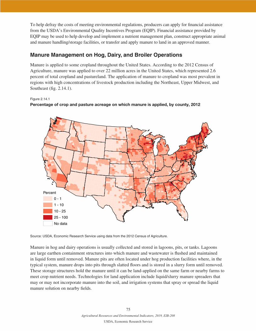
Agricultural Resources and Environmental Indicators, 2019, EIB-208
USDA, Economic Research Service
75
To help defray the costs of meeting environmental regulations, producers can apply for financial assistance from the USDA’s Environmental Quality Incentives Program (EQIP). Financial assistance provided by EQIP may be used to help develop and implement a nutrient management plan, construct appropriate animal and manure handling/storage facilities, or transfer and apply manure to land in an approved manner.
Manure Management on Hog, Dairy, and Broiler Operations
Manure is applied to some cropland throughout the United States. According to the 2012 Census of Agriculture, manure was applied to over 22 million acres in the United States, which represented 2.6 percent of total cropland and pastureland. The application of manure to cropland was most prevalent in regions with high concentrations of livestock production including the Northeast, Upper Midwest, and Southeast (fig. 2.14.1).
Figure 2.14.1
Percentage of crop and pasture acreage on which manure is applied, by county, 2012
Percent
0 - 1
1 - 10
10 - 25
25 - 100
No data
Source: USDA, Economic Research Service using data from the 2012 Census of Agriculture.
Manure in hog and dairy operations is usually collected and stored in lagoons, pits, or tanks. Lagoons are large earthen containment structures into which manure and wastewater is flushed and maintained in liquid form until removed. Manure pits are often located under hog production facilities where, in the typical system, manure drops into pits through slatted floors and is stored in a slurry form until removed. These storage structures hold the manure until it can be land-applied on the same farm or nearby farms to meet crop nutrient needs. Technologies for land application include liquid/slurry manure spreaders that may or may not incorporate manure into the soil, and irrigation systems that spray or spread the liquid manure solution on nearby fields.

Agricultural Resources and Environmental Indicators, 2019, EIB-208
USDA, Economic Research Service
76
The different systems for manure management have very different impacts on the nutrient content of the manure, primarily nitrogen, and thus on the amount of land needed to spread manure. For example, handling manure in pit or tank storage and using slurry spreaders to inject the manure into the soil manages the manure for its potential fertilizer value. This system is designed to retain manure nitrogen for crop use, and thus it requires more land on which to apply the manure if the operation is following a nitro-gen-based nutrient management plan. In contrast, handling manure from lagoon storage and distributing it with irrigation increases the release of nitrogen into the atmosphere, reducing the manure’s nitrogen content and requiring less land for application.
On broiler operations, manure is typically collected along with bedding material (e.g., wood shavings) and feathers when houses are cleaned. The mixture of bedding and manure (called litter) is relatively dry, which makes it easier and cheaper to store and transport than hog and cow manure. When a poultry house is cleaned out, the litter can be immediately spread on a field or stored for later applications. When stored, litter is often kept in a shed to reduce rainwater runoff of nutrients.
On some livestock operations, manure is directly deposited on the fields by grazing animals. However, on most confined livestock operations, manure is collected and then spread on the operation’s own fields or removed from the operation and spread on nearby farmland. The amount of manure that is applied onfarm versus removed depends on how much cropland the farm controls, the nutrient uptake of the crops grown on the farm, and the demand for manure on nearby farms.
The USDA’s Agricultural Resource Management Survey (ARMS), which focuses on different types of livestock producers every 4 or 5 years, provides detailed information about farm production practices, including manure management.1 Based on the 2009 ARMS, 78 percent of hog operations applied manure on their own operations—with about an equal share applying in solid, liquid, or slurry form (table 2.14.1). The average hog operation applied manure to 105 acres of land, which represents about a fifth of the average operation’s cropland. About 21 percent of hog operations removed manure from their operations, with most giving it away. Only 5 percent of hog farms sold manure, reflecting weak demand for hog manure in regions where hogs are produced.
Dairy operations were more likely than hog operations to use manure on their own operations. In 2010, 95 percent of dairies applied manure onfarm, mostly in solid form. The average dairy applied manure to 156 acres, which represents about half of the dairy sector’s average crop acreage. Only 10 percent of dairies removed manure from their operation, again with most of this given away for free.
In 2011, only about half (52 percent) of broiler operations applied manure onfarm; a large portion of broiler growers have no cropland. Growers who do have cropland apply manure at a high rate; on average, manure is applied on over 90 percent of available crop acres. With little cropland for spreading manure, almost three-quarters of all broiler operations removed some manure from their operation in 2011. Broiler litter is relatively valuable. Almost two-thirds of operations either sold manure or exchanged it for services (such as cleaning out the broiler house).
1Detailed information about manure management was not collected after 2011.

Agricultural Resources and Environmental Indicators, 2019, EIB-208
USDA, Economic Research Service
77
Table 2.14.1
Manure/litter application and removal on livestock operations, 2009-11
Hogs Dairy Broilers
Average per farm
Acres with manure/litter application 105 156 88
Cropland acres 503 316 95
Percent of cropland with manure/litter application 21 49 93
Percent of farms
Applied manure/litter onfarm 78 95 52
Solid 29 80 n.a.
Liquid 27 31 n.a.
Slurry 36 20 n.a.
Manure deposited on fields/pasture 4 10 n.a.
Removed manure/litter from operation 21 10 72
Sold manure/litter 5 2 34
Litter given in exchange for service n.a. n.a. 31
Manure/litter given away for free 16 7 10
Paid for manure/litter removal 2 1 3
Note: n.a. = Not asked on survey. Source: USDA, Economic Research Service and National Agricultural Statistics Service, Agricultural Resource Management
Survey, 2009 (hogs), 2010 (dairy), 2011 (broilers).
Manure Nutrient Management Practices
In addition to deciding whether to apply manure onfarm, growers must decide how much manure to apply to their crops. A nutrient management plan (NMP), which can be voluntary or required by statute, specifies a set of nutrient management practices that a farmer should take to match applied manure and commercial fertilizer nutrients with the absorptive capacity of the land and crops. About two-thirds of broiler operations had an NMP in 2011, compared with 54 percent of hog operations (2009) and 41 percent of dairies (2010, table 2.14.2). Manure nutrient testing, a practice required as part of many State-mandated manure management plans, was employed by about a third of hog and broiler operations and 22 percent of dairy operations.
Farmers apply commercial fertilizer to crops in addition to manure if the manure nutrients do not meet the nutritional needs of the crops. Testing the nutrient content of manure can save costs by avoiding the over-application of supplemental commercial fertilizer. About 43 percent of all dairy operations adjusted their fertilizer nutrients, compared to 31 percent of hog operations and 14 percent of broiler operations.
Some hog and dairy operations adjusted the nutrient content of manure via modification to their feed formula or feeding schedule, typically to reduce the nitrogen or phosphorus content of the manure. This allows the same amount of manure to be spread over a smaller amount of land while providing the same amount of nutrients. Adjusting the nutrient content of manure via feed was practiced by a third of hog operations, but only 7 percent of dairy farms.

Agricultural Resources and Environmental Indicators, 2019, EIB-208
USDA, Economic Research Service
78
EQIP payments for manure management were used primarily for installing manure handling and storage facilities, manure hauling, and application or for a nutrient management plan (development, testing, and recordkeeping). EQIP payments were not common: the share of hog, dairy and broiler operations that received these payments ranged from 2 to 4 percent over 2009-11 (see chapter 3.24, “Working Lands”).
Table 2.14.2
Percent of farms with manure/litter management practices, 2009-11
Hogs Dairy Broilers
Has a nutrient management plan 54 41 66
Tested manure/litter for N or P content 37 22 31
Adjusted commercial fertilizer to account for manure/litter nutrients (N or P) 31 43 14
Adjusted nutrient content of manure via feed formula or feeding schedule 33 7 n.a.
Received EQIP payments for manure management 3 4 2
Note: n.a. = Not asked on survey. N = nitrogen; P = phosphorus.Source: USDA, Economic Research Service and National Agricultural Statistics Service, Agricultural Resource Management Survey, 2009 (hogs), 2010 (dairy), 2011 (broilers).
References
Key, N., W. McBride, M. Ribaudo, and S. Sneeringer. 2011. Trends and Developments in Hog Manure Management. EIB-81. U.S. Department of Agriculture, Economic Research Service, Sept.
MacDonald, James M. 2014. Technology, Organization, and Financial Performance in U.S. Broiler Pro-duction, EIB-126. U.S. Department of Agriculture, Economic Research Service, June.
Ribaudo, Marc, Jeffrey Savage, and Marcel Aillery. 2014. An Economic Assessment of Policy Options To Reduce Agricultural Pollutants in the Chesapeake Bay, ERR-166, U.S. Department of Agriculture, Economic Research Service, June.
Stacy Sneeringer. 2016. Comparing Participation in Nutrient Trading by Livestock Operations to Crop Producers in the Chesapeake Bay Watershed. ERR-216. U.S. Department of Agriculture, Economic Research Service, Sept.

Agricultural Resources and Environmental Indicators, 2019, EIB-208
USDA, Economic Research Service
79
Chapter 2.15—Antibiotic Use in U.S. Livestock Production
Stacy Sneeringer and Maria Bowman
• By the end of 2017, 44 percent of U.S. broiler chickens were raised without any antibiotics.
• Between 2004 and 2015, the share of finishing hogs sold or removed from operations reporting that they did not know or did not report whether antibiotics were used for growth promotion rose from 7 percent to 35 percent.
• Use of antibiotics for purposes other than disease treatment is associated with a 1- to 3-percent increase in the productivity of hog and broiler operations.
The animal agriculture sector is a major user of antibiotic drugs for disease treatment, disease control, and disease prevention. These drugs are pivotal for animal health and farm productivity, but many of the antibiotics used on the farm are in the same classes as those used in human medicine. Agricultural use of antibiotics important for disease treatment in human medicine— called “medically important” antibiotics by the FDA1—is an increasing source of public health concern. Routine use of antibiotics, in humans or animals, can promote antimicrobial resistance, such that antibiotics fail to contain bacterial infections. The U.S. Centers for Disease Control and Prevention (CDC) estimates that over 2 million people in the United States annually become ill from resistant infections, with at least 23,000 dying (CDC, 2013). Other estimates suggest that by 2050, antimicrobial resistance will result in more deaths than cancer worldwide (Review on Antimicrobial Resistance, 2016). While antibiotics administered to livestock have been linked to human health risks, the extent of these risks remains a matter of debate.
Concerns over antibiotic resistance have led to calls to use the drugs more judiciously in all settings, and to examine alternatives to their use. In 2017, new U.S. Food and Drug Administration (FDA) rules went into effect making it illegal to provide medically important antibiotics in feed or water to livestock for production purposes such as growth promotion (U.S. FDA, 2012 and 2013). These new requirements now compel veterinarians to oversee all use of in-feed or in-water medically important antibiotics in livestock, rather than having some available over the counter. Consumers and major retailers also are increasingly demanding livestock products resulting from animals that never received any antibiotics for any purpose. In response, several major food retailers have placed restrictions on the use of antibiotics for production purposes by their meat suppliers (Pew Charitable Trusts, 2015). Changes in antibiotic use will lead to a series of adjustments in animal agriculture as producers change production practices, with potential reper-cussions for prices and volumes in livestock markets.
Use of Antibiotics in the Livestock Sectors
Reasons for antibiotic use, extent of their use, who makes the decision to use them, how restrictions on use would be felt in the industry, and how policies could be implemented all depend on the structure and organization of livestock production.
1Nonmedically important antibiotics are those not used in human medicine. The predominant type of these is ionophores.
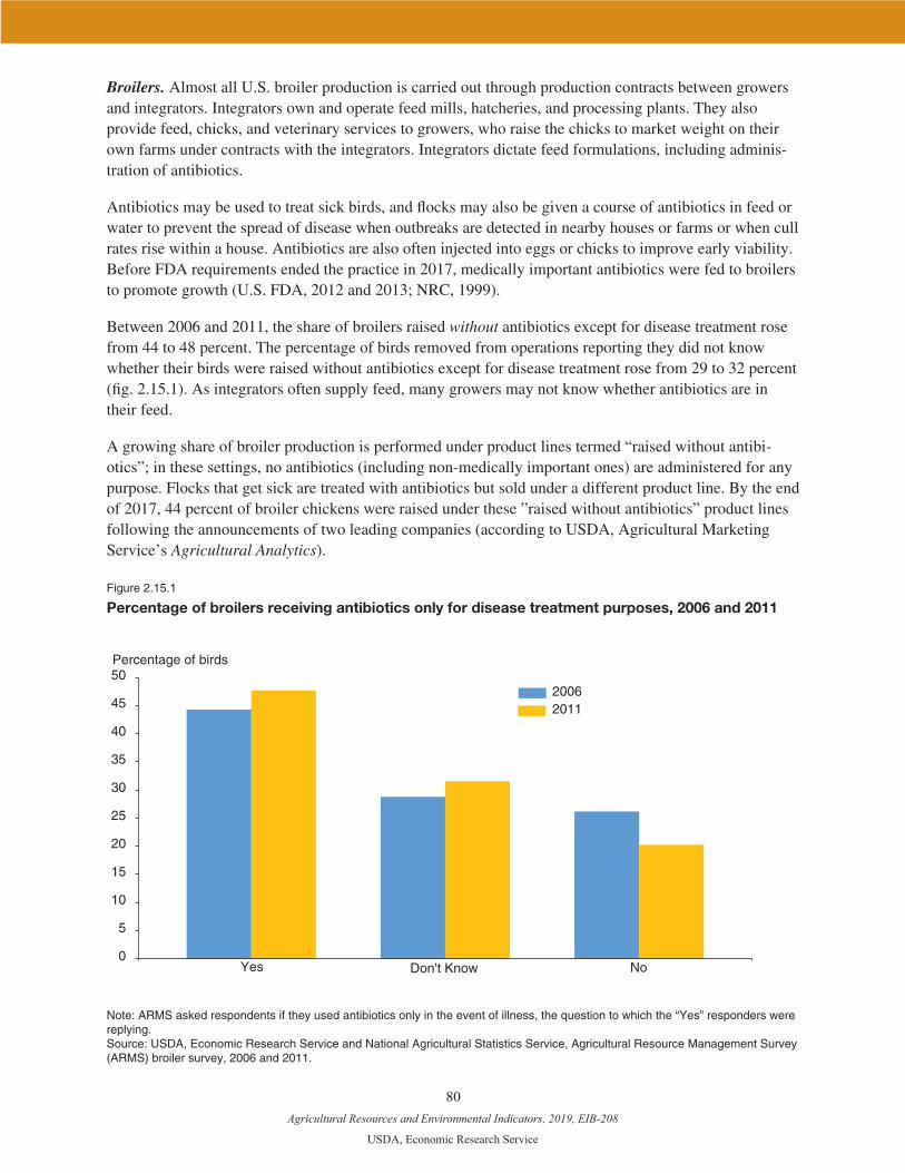
Agricultural Resources and Environmental Indicators, 2019, EIB-208
USDA, Economic Research Service
80
Broilers. Almost all U.S. broiler production is carried out through production contracts between growers and integrators. Integrators own and operate feed mills, hatcheries, and processing plants. They also provide feed, chicks, and veterinary services to growers, who raise the chicks to market weight on their own farms under contracts with the integrators. Integrators dictate feed formulations, including adminis-tration of antibiotics.
Antibiotics may be used to treat sick birds, and flocks may also be given a course of antibiotics in feed or water to prevent the spread of disease when outbreaks are detected in nearby houses or farms or when cull rates rise within a house. Antibiotics are also often injected into eggs or chicks to improve early viability. Before FDA requirements ended the practice in 2017, medically important antibiotics were fed to broilers to promote growth (U.S. FDA, 2012 and 2013; NRC, 1999).
Between 2006 and 2011, the share of broilers raised without antibiotics except for disease treatment rose from 44 to 48 percent. The percentage of birds removed from operations reporting they did not know whether their birds were raised without antibiotics except for disease treatment rose from 29 to 32 percent (fig. 2.15.1). As integrators often supply feed, many growers may not know whether antibiotics are in their feed.
A growing share of broiler production is performed under product lines termed “raised without antibi-otics”; in these settings, no antibiotics (including non-medically important ones) are administered for any purpose. Flocks that get sick are treated with antibiotics but sold under a different product line. By the end of 2017, 44 percent of broiler chickens were raised under these ”raised without antibiotics” product lines following the announcements of two leading companies (according to USDA, Agricultural Marketing Service’s Agricultural Analytics).
Figure 2.15.1
Percentage of broilers receiving antibiotics only for disease treatment purposes, 2006 and 2011
0
5
10
15
20
25
30
35
40
45
5020062011
Yes Don't Know No
Percentage of birds
Note: ARMS asked respondents if they used antibiotics only in the event of illness, the question to which the “Yes” responders were replying. Source: USDA, Economic Research Service and National Agricultural Statistics Service, Agricultural Resource Management Survey (ARMS) broiler survey, 2006 and 2011.

Agricultural Resources and Environmental Indicators, 2019, EIB-208
USDA, Economic Research Service
81
Hogs. Hog production has become increasingly vertically integrated and specialized in terms of the animal lifecycle. Integrators provide contract growers with feed, veterinary services, and animals. Contracted sow operations farrow young pigs, which are shipped to nursery operations. There they are raised to feeder weights and then shipped to finishing operations. After being fed to market weights, inte-grators either ship the hogs to their own packing plants or sell them to others.
Hogs may be treated for diseases with antibiotics at any point in their lifecycle, but an especially risky time occurs in the pre-weaning and nursery stages. In 2012, 10 percent of pre-weaning piglet deaths were caused by scours (another name for diarrhea), an illness frequently treated with antibiotics. In the finishing stages, respiratory problems are the most prevalent disease-induced causes of death (75 percent); these instances are also treated with antibiotics (USDA, APHIS, 2015).
Before the FDA requirements ended the practice in 2017, antibiotics were fed to both young (nursery) pigs as well as market (finishing) hogs to promote growth. Between 2004 and 2015, the share of finishing hogs sold or removed2 from operations reporting that they did not administer antibiotics for growth promotion declined from 41 percent to 31 percent (fig. 2.15.2). Over the same time period, the share of operations stating they did not know—or did not report—whether antibiotics were administered for growth promotion rose by 28 percentage points. This was coupled with a comparable decline in hogs raised at operations reporting that they did use antibiotics for growth promotion. Thus, for finishing hogs, producers seemingly became less willing or able to report on their use of antibiotics for growth promotion between 2004 and 2015.
Figure 2.15.2
Percentage of hogs sold or removed receiving antibiotics for growth promotion, 2004, 2009and 2015
Percentage of hogs
0
10
20
30
40
50
60
70
Yes YesNo NoDon't know or missing
Don't knowor missing
Nursery hogs Finishing hogs
200420092015
Source: USDA, Economic Research Service and National Agricultural Statistics Service, Agricultural Resource Management Survey, 2004, 2009, and 2015.
2Independent hog producers sell animals. Contracted hog producers have hogs “removed” from their facilities. Hence the phrase “sold or removed.”

Agricultural Resources and Environmental Indicators, 2019, EIB-208
USDA, Economic Research Service
82
Trends for nursery hogs are less easy to interpret. The share of nursery hogs sold or removed from opera-tions that did not administer antibiotics for growth fell from 65 to 51 percent between 2004 and 2009, but then rose to 55 percent between 2009 and 2015. The share of operations stating that they did not know or report whether antibiotics were administered rose from 6 to 17 percent (2015), while the share of nursery hog operations reporting that they did use antibiotics for growth promotion remained around 29 percent. Because of these shifts, it is difficult to tell whether use of growth-promoting antibiotics in nursery pig production rose or fell between 2004 and 2015.
Beef cattle. Beef cattle production can be divided into two stages. On cow-calf operations, calves are birthed and raised until weaning. In 2007/2008, nearly 16 percent of cow-calf operations reported adding antibiotics (inclusive of non-medically important antibiotics) to cattle feed to prevent disease and/or promote growth (USDA, APHIS, 2012).
On stocker, backgrounding, and feedlot operations, cattle are fed to slaughter weight. Animals are often shipped long distances to these operations. Co-mingling of cattle from various locations increases the threat of disease spread, so animals often receive preventive injections of antibiotics upon arrival. In 2011, a quarter of cattle at large-scale feedlots received injected antibiotics (USDA, APHIS, 2012). Nearly half of cattle at large-scale feedlots received medically important antibiotics in feed (USDA, APHIS, 2013).
Dairy. Unlike hogs or broilers, dairies do not operate under production contracts. Dairy operators often retain female cows for their entire lifecycle, while selling male calves for beef. Antibiotics are used on dairy farms to treat and prevent disease, but they also have been used in heifer rations for growth promo-tion. Diarrheal and respiratory problems are frequent in preweaned dairy calves. To help prevent these illnesses, dairy operations fed 40 percent of pre-weaned heifers medicated milk replacer in 2014 (USDA, APHIS, 2016a).
After heifers are bred and give birth, they may contract diseases or disorders that are often treated with antibiotics. In 2014, 93 percent of dairy operations provided antibiotics for prevention of intramammary infections between lactation periods (USDA, APHIS, 2016b).
Notably, the FDA has established minimum intervals between the last dose of antimicrobials and the time of slaughter to allow antibiotic residues in meat to reach levels safe for human consumption (U.S. FDA, 2014). Likewise, if dairy cows have been treated with antibiotics, they must be withdrawn for a time before their milk can be sold into the food chain.
Economics of Reducing Antibiotic Use
Antibiotics may reduce the use of other inputs (such as feed) and lower morbidity and mortality. If the gains from using antibiotics outweigh the costs, then antibiotic use can increase livestock productivity and efficiency. Indirectly, antibiotics may influence the scale and type of production; if antibiotics reduce the amount of space needed per animal, then more animals can be raised per square foot.
Reducing antibiotic use may require adjustments to production processes. Farm operators may need to provide more feed to reach production targets, but they may also use other animal drugs, feed supple-ments, administer vaccines, alter sanitation practices, change genetic lines, or modify housing environ-ments through capital investments. Such adjustments influence the financial outcomes from reducing antibiotic use and may also affect animal health and environmental outcomes.

Agricultural Resources and Environmental Indicators, 2019, EIB-208
USDA, Economic Research Service
83
Reducing use of antibiotics may yield higher production costs, which can lead to higher prices and lower market supply. Use of antibiotics for purposes other than disease treatment is associated with a 1- to 3-percent increase in productivity on hog and broiler operations. The increase in the cost of production from ceasing antibiotic use is estimated to lead to an increase of 1 percent in wholesale prices and a drop in output of less than 1 percent (Sneeringer et al., 2015).
References
National Research Council (NRC). 1999. The Use of Drugs in Food Animals: Benefits and Risks. Wash-ington, DC: National Academies Press.
Pew Charitable Trusts. 2015. “Top food companies moving away from overuse of antibiotics on industrial farms.” March 9.
Review on Antimicrobial Resistance. 2016. Tackling Drug-Resistant Infections Globally: Final Report and Recommendations. Chaired by Jim O’Neill. May.
Sneeringer, Stacy, James MacDonald, Nigel Key, William McBride, and Ken Mathews. 2015. Economics of Antibiotic Use in U.S. Livestock Agriculture. ERR-200. U.S. Department of Agriculture, Economic Research Service, Nov.
U.S. Centers for Disease Control and Prevention (CDC). 2013. Antibiotic Resistance Threats in the Unit-ed States.
U.S. Department of Agriculture (USDA), Agricultural Marketing Service (AMS), Agricultural Analytics. Michael Sheats, personal communication.
U.S. Department of Agriculture (USDA), Animal and Plant Health Inspection Service (APHIS). 2016a. Dairy 2014: Dairy Cattle Management Practices in the United States, 2014. Fort Collins, CO. #692.0216.
U.S. Department of Agriculture (USDA), Animal and Plant Health Inspection Service (APHIS). 2016b. Dairy 2014: Milk Quality, Milking Procedures, and Mastitis on U.S. Dairies, 2014. Fort Collins, CO. #704.0916.
U.S. Department of Agriculture (USDA), Animal and Plant Health Inspection Service (APHIS). 2015. Swine 2012, Part I: Baseline Reference of Swine Health and Management in the United States, 2012. Fort Collins, CO. #663.0115.
U.S. Department of Agriculture (USDA), Animal and Plant Health Inspection Service (APHIS). 2012. Beef 2007-08: Antimicrobial Drug Use and Antimicrobial Resistance on U.S. Cow-calf Operations, 2007-08. Fort Collins, CO. #577.0212.
U.S. Department of Agriculture (USDA), Animal and Plant Health Inspection Service (APHIS). 2013. “Part I: Management Practices on U.S. Feedlots with a Capacity of 1,000 or More Head,” Feedlot 2011. Fort Collins, CO. #626.0313
U.S. Food and Drug Administration (FDA). 2012. Guidance for Industry: The Judicious Use of Medically Important Antimicrobial Drugs in Food-Producing Animals. Department of Health and Human Ser-vices Center for Veterinary Medicine. #209.
U.S. Food and Drug Administration (FDA). 2013. Guidance for Industry: New Animal Drugs and New Animal Drug Combination Products Administered in or on Medicated Feed or Drinking Water of Food-Producing Animals: Recommendations for Drug Sponsors for Voluntarily Aligning Product Use Conditions with GFI #209. #213.
U.S. Food and Drug Administration (FDA). 2014. From an Idea to the Marketplace: The Journey of an Animal Drug through the Approval Process. June. Department of Health and Human Services.

Group 3: Natural Resources and Conservation
Agricultural Resources and Environmental Indicators, 2019, EIB-208
USDA, Economic Research Service
84
Chapter 3.16—Farm-Level Adaptation to Drought Risk
Steven Wallander and Andrew Crane-Droesch
• Exposure to drought risk varies considerably across the country. In some Western States, agricultur-al producers experience a severe or extreme drought in 1 out of every 3 years, on average, versus 1 out of 5 years in the Midwest and Northeast.
• Participation in voluntary conservation programs is influenced by regional differences in drought risk. Producers in higher risk regions are more likely to participate in EQIP (Environmental Quality Incentives Program) contracts that include irrigation efficiency improvements or water conservation.
• Irrigation can be an important source of drought resilience, but drought often leads to severe curtailment of surface-water supplies for irrigation. In some areas, irrigators can offset reduced surface-water availability through increased groundwater pumping, which can extend droughts’ long-term impacts through depleted groundwater levels.
Drought Risk
The risk of drought is a concern for agricultural producers throughout the county. Drought—a reduc-tion in water availability due to a combination of low precipitation and high temperatures—can reduce productivity and lead to severe losses in farm income. Droughts are measured both in terms of duration and severity, and their impact can be dependent on their timing.
A variety of policy options address drought, many involving large-scale investments in infrastructure or major changes in water allocation that are beyond the agricultural sector’s control (Schwabe and Connor, 2012). This chapter focuses on farm-level decisions that can attenuate the impacts of drought, which can be influenced by existing infrastructure and institutional arrangements.
Drought is the leading driver of production risk in U.S. agriculture (fig. 3.16.1). No other source of production risk—including flooding, early frosts, and pests—is as nationally significant as drought in terms of lost agricultural production and income. A major drought can reduce crop yields, limit planted or harvested acreage, reduce livestock productivity, and increase costs of production inputs such as animal feed and irrigation water.
Group 3: Natural Resources and Conservation

Agricultural Resources and Environmental Indicators, 2019, EIB-208
USDA, Economic Research Service
85 85
Figure 3.16.1
Drought is the largest cause of crop insurance indemnities and disaster payments, 1970-2016
Percent of crop cash reciepts
0
2
4
6
8
10
12
1970
1971
1972
1973
1974
1975
1976
1977
1978
1979
1980
1981
1982
1983
1984
1985
1986
1987
1988
1989
1990
1991
1992
1993
1994
1995
1996
1997
1998
1999
2000
2001
2002
2003
2004
2005
2006
2007
2008
2009
2010
2011
2012
2013
2014
2015
2016
Drought indemnity Drought disaster assistance Other indemnity Other disaster assistance
Note: Total payments have been converted into percentage of cash crop receipts using ERS annual farm income tables.Source: USDA, Economic Research Service using cause-of-loss data from USDA’s Risk Management Agency and disaster assis-tance data from USDA’s annual reports on Commodity Credit Corporation expenditures.
Regions differ in how frequently they experience severe drought. Some regions, such as parts of the Midwest, Northeast, and coastal Northwest, have experienced severe or extreme drought for about 1 of every 5 years, on average, from 1900 to 2016. Other areas face higher drought risk. For example, areas in the Southwest, Southeast, Northern High Plains, and intermountain West have had severe or extreme drought about once every 3 years (fig. 3.16.2).
Precipitation and temperature vary widely by region, so climatologists measure droughts relative to local climate conditions. For example, the conditions associated with an extreme drought in central Ohio can look like average, non-drought conditions in semi-arid western Kansas. Farmers in different regions tailor their crop choices, production systems, and decisions on inputs (like how much fertilizer to apply) based largely on average weather conditions in their area—which makes them vulnerable when those conditions change.
Adaptation to Drought Risk
In general, adaptation is the process of altering behaviors and characteristics to improve suitability to a given environment. For example, increased drought risk stemming from climate change may prompt farmers to alter their production practices or investments.
Adaptive changes are generally taken to minimize damages to livelihoods stemming from adverse events, and/or to capitalize on any opportunities presented. Almost all farmer actions can be viewed as adaptation, because the physical, biological, and economic environment in which farmers operate changes continuously. The likelihood of increased risk and severity of drought—defined both by temperature and precipitation—is one of many factors to which farmers will adapt in coming years and decades (IPCC, 2014).

Agricultural Resources and Environmental Indicators, 2019, EIB-208
USDA, Economic Research Service
86 86
Figure 3.16.2
Drought risk reflects frequency of severe drought and varies regionally, 1900-2016
19-25 26-30 31-35 36-46 47-57
Drought frequency
Years of drought from 1900-2016
Note: Drought frequency is the number of years when at least 1 summer month (June, July, or August) had moderate or worse drought (PMDI ≤ -2.00).Source: USDA, Economic Research Service using historical data by climate district from the National Oceanic and Atmospheric Administration, Palmer Modified Drought Index (PMDI).
Adaptation may be shortrun or longrun. Shortrun adaptation generally involves minimal fixed or sunk costs and often provides drought remediation for only one or two seasons. For example, shifting planted acreage from a drought-sensitive to a drought-tolerant crop would be a short-term adaptation to increased drought risk. Likewise, a shift into drought-sensitive crops would be adaptive for a farmer who is less exposed to drought (if prices of the drought-sensitive crop are expected to increase in response to changes in supply).
Longrun adaptations to increased drought risk will generally be more expensive and less reversible, but sometimes more effective. For example, farmers may buy or sell land in response to changing expecta-tions of its future value, or farmers could install water-saving infrastructure on their farms, such as check-dams on tile drainage systems. ERS research has shown that farmers in higher risk drought regions are more likely to enroll in the Environmental Quality Incentives Program (EQIP) for financial assistance that supports drought-mitigating practices (Wallander et al., 2013).
Irrigation and Drought Adaptation
Irrigation can be a straightforward response to drought. When available precipitation cannot meet crop water requirements, irrigators can add water to meet the demand if an adequate water supply is avail-able. However, expanding irrigated acreage as a response to increased drought risk may not be feasible. Irrigation levels are constrained by water availability, which is a function of climate, geology, invest-ments in the infrastructure required to store and transport water, and water allocation institutions. Irrigated
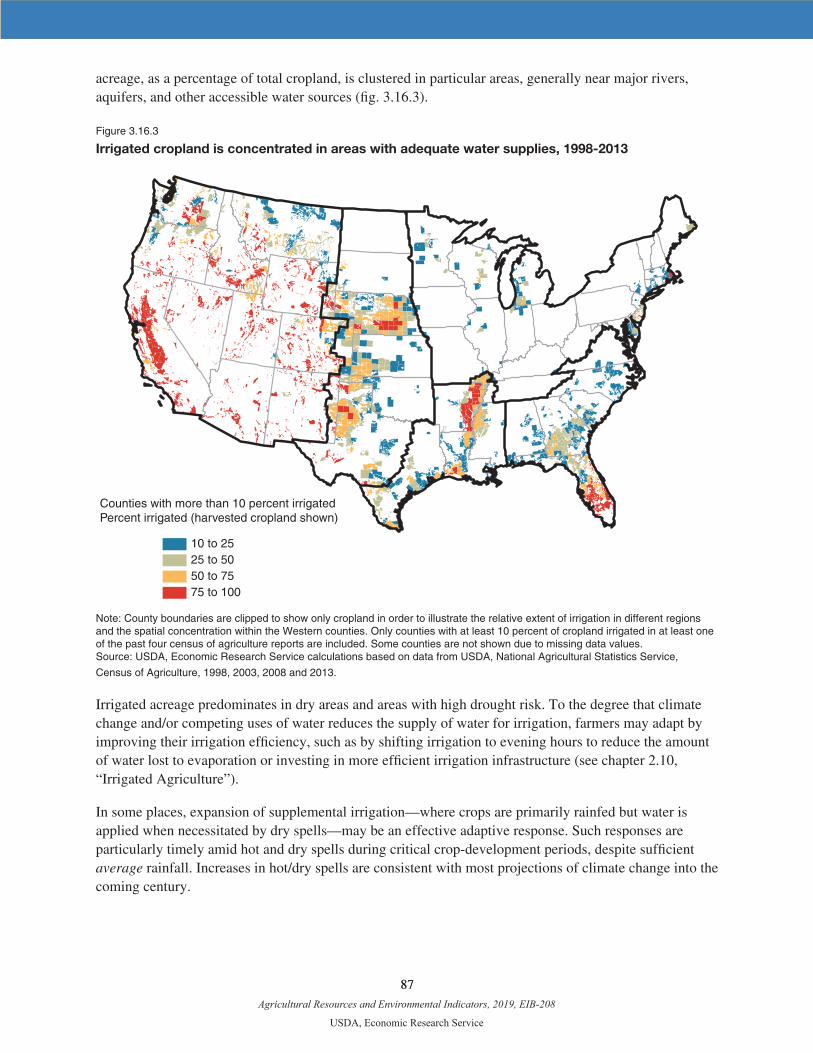
Agricultural Resources and Environmental Indicators, 2019, EIB-208
USDA, Economic Research Service
87 87
acreage, as a percentage of total cropland, is clustered in particular areas, generally near major rivers, aquifers, and other accessible water sources (fig. 3.16.3).
Figure 3.16.3
Irrigated cropland is concentrated in areas with adequate water supplies, 1998-2013
10 to 2525 to 5050 to 7575 to 100
Counties with more than 10 percent irrigatedPercent irrigated (harvested cropland shown)
Note: County boundaries are clipped to show only cropland in order to illustrate the relative extent of irrigation in different regions and the spatial concentration within the Western counties. Only counties with at least 10 percent of cropland irrigated in at least one of the past four census of agriculture reports are included. Some counties are not shown due to missing data values.Source: USDA, Economic Research Service calculations based on data from USDA, National Agricultural Statistics Service,
Census of Agriculture, 1998, 2003, 2008 and 2013.
Irrigated acreage predominates in dry areas and areas with high drought risk. To the degree that climate change and/or competing uses of water reduces the supply of water for irrigation, farmers may adapt by improving their irrigation efficiency, such as by shifting irrigation to evening hours to reduce the amount of water lost to evaporation or investing in more efficient irrigation infrastructure (see chapter 2.10, “Irrigated Agriculture”).
In some places, expansion of supplemental irrigation—where crops are primarily rainfed but water is applied when necessitated by dry spells—may be an effective adaptive response. Such responses are particularly timely amid hot and dry spells during critical crop-development periods, despite sufficient average rainfall. Increases in hot/dry spells are consistent with most projections of climate change into the coming century.
Agricultural Resources and Environmental Indicators, 2019, EIB-208
USDA, Economic Research Service
88 88
Farmers generally have limited control over the availability of groundwater or surface-water reserves for irrigation. Irrigation reduces drought vulnerability in many areas by allowing farmers to augment precip-itation where sufficient groundwater is available. In other areas, surface-water irrigation is possible, but its infrastructure is costly. Some irrigators rely almost exclusively on large aquifers, such as the Ogallala Aquifer in the High Plains and the Mississippi Embayment in the southern Mississippi River region. Many of these aquifers have recently been subjected to severe overdraft, which significantly reduces the availability of groundwater as a buffer to drought. In the intermountain West, many irrigators draw on both groundwater and surface-water supplies, which can allow users to apply excess surface water in wet years to replenish groundwater reserves that are overdrafted in dry years.
In California and other Western States, surface-water supplies are highly vulnerable to drought. Reservoir storage systems help economize on irrigation supplies during periods of reduced stream flows, providing a buffer against short-term drought. However, reliance on surface water for irrigation creates its own form of drought vulnerability. Prolonged drought generally reduces the quantity of surface water delivered, compromising farm production systems that depend heavily on surface water for irrigation.
Furthermore, most aspects of water allocation are under the purview of State laws. Many States have established institutions for allocating water rights among competing uses and users based on seniority (“prior appropriation” water rights). When water availability is low, senior water rights holders in those States are first in line for water allocation. Water is delivered fully in order of seniority until allocation limits are reached, and then remaining rights holders receive no deliveries. This makes irrigators with less senior water rights particularly vulnerable during periods of drought. In some areas, States and local water districts have established markets to allow for the trading of water rights.
Tile Drainage and Adaptation
Tile drainage (fig. 3.16.4) has traditionally been installed to address problems of excess water, rather than drought. Tile drains help farmers to quickly remove excess water from the soil profile, allowing them to work the fields and avoid waterlogging. However, major droughts (e.g., 1956, 1988, and 2012) have led to yield losses in areas that are tile drained since these areas do not typically have irrigation. Modified tile drainage may allow some producers to temporarily restrict flow, if they are able to temporarily close or restrict the systems and retain more water in the soil profile as a safeguard against drought.
Soil Health and Adaptation
Many farms may lack the water supply to use irrigation as a drought adaptation strategy, or the slope and soil profile to make tile drainage effective. However, all farms may improve their resilience to drought by investing in soil health.
Soil organic matter provides numerous agro-ecological functions and is a prime indicator of overall soil health (see chapter 3.19, “Soil Health”). Investing in soil health practices that increase soil organic matter can enable the soil profile to retain more water while also improving infiltration and reducing runoff during intense rain events. Effective soil organic matter practices vary by region and production system, but include conservation tillage and cover cropping. Both approaches encourage soil carbon stocks to accumulate faster than their natural rate of decomposition. While the economics of these systems are highly contextual and not fully understood, they may constitute an important adaptive strategy in many areas.

Agricultural Resources and Environmental Indicators, 2019, EIB-208
USDA, Economic Research Service
89 89
Figure 3.16.4 Tile drainage is most common in regions that typically lack irrigation, 2012
0 to 1 1 to 55 to 10 10 to 5050 to 100
Cropland in county tile drained
Percent
Note: County boundaries are clipped to show only cropland to illustrate the relative extent of irrigation in different regions and the spatial concentration within the Western counties.Source: USDA, Economic Research Service calculations based on data from USDA, National Agricultural Statistics Service, 2013 Census of Agriculture.
Conclusion
A variety of options are available to farmers for adapting to drought risk. Few of these options will completely eliminate risk exposure, and almost all are constrained by existing institutional arrangements, public policies, and infrastructure investments. Drought adaptation includes not only irrigation but also tile drainage and measures to promote soil health.
References
Intergovernmental Panel on Climate Change (IPCC). 2014. Climate Change 2014–Impacts, Adaptation and Vulnerability: Regional Aspects. Cambridge University Press.
U.S. Department of Agriculture, National Agricultural Statistics Service. 2012. Census of Agriculture. U.S. Department of Agriculture, Natural Resources Conservation Service. 2017. Soil Survey Geographic
(SSURGO) Database. Schwabe, Kurt A., and Jeffrey D. Connor. 2012. “Drought Issues in Semi-arid and Arid Environments,”
Choices 27(3).Wallander, Steve, Marcel Aillery, Daniel Hellerstein, and Michael S. Hand. 2013. The Role of Conser-
vation Programs in Drought Risk Adaptation. ERR-148. U.S. Department of Agriculture, Economic Research Service.
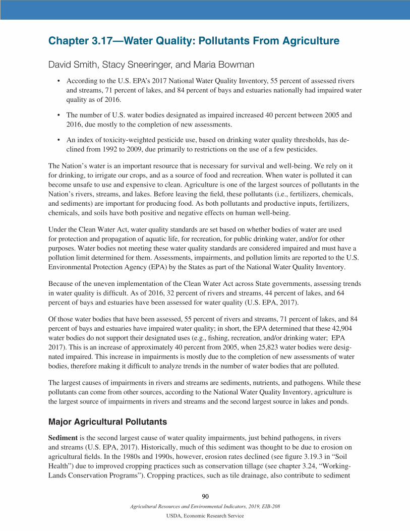
Agricultural Resources and Environmental Indicators, 2019, EIB-208
USDA, Economic Research Service
90 90
Chapter 3.17—Water Quality: Pollutants From Agriculture
David Smith, Stacy Sneeringer, and Maria Bowman
• According to the U.S. EPA’s 2017 National Water Quality Inventory, 55 percent of assessed rivers and streams, 71 percent of lakes, and 84 percent of bays and estuaries nationally had impaired water quality as of 2016.
• The number of U.S. water bodies designated as impaired increased 40 percent between 2005 and 2016, due mostly to the completion of new assessments.
• An index of toxicity-weighted pesticide use, based on drinking water quality thresholds, has de-clined from 1992 to 2009, due primarily to restrictions on the use of a few pesticides.
The Nation’s water is an important resource that is necessary for survival and well-being. We rely on it for drinking, to irrigate our crops, and as a source of food and recreation. When water is polluted it can become unsafe to use and expensive to clean. Agriculture is one of the largest sources of pollutants in the Nation’s rivers, streams, and lakes. Before leaving the field, these pollutants (i.e., fertilizers, chemicals, and sediments) are important for producing food. As both pollutants and productive inputs, fertilizers, chemicals, and soils have both positive and negative effects on human well-being.
Under the Clean Water Act, water quality standards are set based on whether bodies of water are used for protection and propagation of aquatic life, for recreation, for public drinking water, and/or for other purposes. Water bodies not meeting these water quality standards are considered impaired and must have a pollution limit determined for them. Assessments, impairments, and pollution limits are reported to the U.S. Environmental Protection Agency (EPA) by the States as part of the National Water Quality Inventory.
Because of the uneven implementation of the Clean Water Act across State governments, assessing trends in water quality is difficult. As of 2016, 32 percent of rivers and streams, 44 percent of lakes, and 64 percent of bays and estuaries have been assessed for water quality (U.S. EPA, 2017).
Of those water bodies that have been assessed, 55 percent of rivers and streams, 71 percent of lakes, and 84 percent of bays and estuaries have impaired water quality; in short, the EPA determined that these 42,904 water bodies do not support their designated uses (e.g., fishing, recreation, and/or drinking water; EPA 2017). This is an increase of approximately 40 percent from 2005, when 25,823 water bodies were desig-nated impaired. This increase in impairments is mostly due to the completion of new assessments of water bodies, therefore making it difficult to analyze trends in the number of water bodies that are polluted.
The largest causes of impairments in rivers and streams are sediments, nutrients, and pathogens. While these pollutants can come from other sources, according to the National Water Quality Inventory, agriculture is the largest source of impairments in rivers and streams and the second largest source in lakes and ponds.
Major Agricultural Pollutants
Sediment is the second largest cause of water quality impairments, just behind pathogens, in rivers and streams (U.S. EPA, 2017). Historically, much of this sediment was thought to be due to erosion on agricultural fields. In the 1980s and 1990s, however, erosion rates declined (see figure 3.19.3 in “Soil Health”) due to improved cropping practices such as conservation tillage (see chapter 3.24, “Working-Lands Conservation Programs”). Cropping practices, such as tile drainage, also contribute to sediment
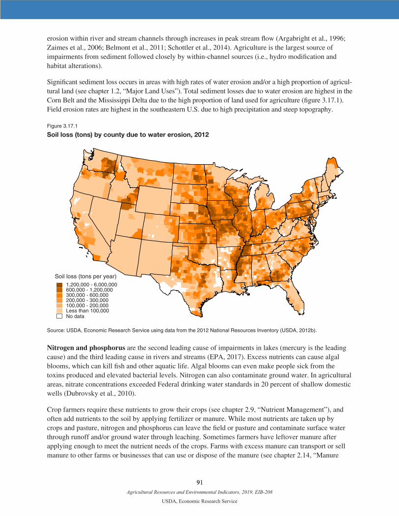
Agricultural Resources and Environmental Indicators, 2019, EIB-208
USDA, Economic Research Service
91 91
erosion within river and stream channels through increases in peak stream flow (Argabright et al., 1996; Zaimes et al., 2006; Belmont et al., 2011; Schottler et al., 2014). Agriculture is the largest source of impairments from sediment followed closely by within-channel sources (i.e., hydro modification and habitat alterations).
Significant sediment loss occurs in areas with high rates of water erosion and/or a high proportion of agricul-tural land (see chapter 1.2, “Major Land Uses”). Total sediment losses due to water erosion are highest in the Corn Belt and the Mississippi Delta due to the high proportion of land used for agriculture (figure 3.17.1). Field erosion rates are highest in the southeastern U.S. due to high precipitation and steep topography.
Figure 3.17.1
Soil loss (tons) by county due to water erosion, 2012
1,200,000 - 6,000,000600,000 - 1,200,000300,000 - 600,000200,000 - 300,000100,000 - 200,000Less than 100,000No data
Soil loss (tons per year)
Source: USDA, Economic Research Service using data from the 2012 National Resources Inventory (USDA, 2012b).
Nitrogen and phosphorus are the second leading cause of impairments in lakes (mercury is the leading cause) and the third leading cause in rivers and streams (EPA, 2017). Excess nutrients can cause algal blooms, which can kill fish and other aquatic life. Algal blooms can even make people sick from the toxins produced and elevated bacterial levels. Nitrogen can also contaminate ground water. In agricultural areas, nitrate concentrations exceeded Federal drinking water standards in 20 percent of shallow domestic wells (Dubrovsky et al., 2010).
Crop farmers require these nutrients to grow their crops (see chapter 2.9, “Nutrient Management”), and often add nutrients to the soil by applying fertilizer or manure. While most nutrients are taken up by crops and pasture, nitrogen and phosphorus can leave the field or pasture and contaminate surface water through runoff and/or ground water through leaching. Sometimes farmers have leftover manure after applying enough to meet the nutrient needs of the crops. Farms with excess manure can transport or sell manure to other farms or businesses that can use or dispose of the manure (see chapter 2.14, “Manure
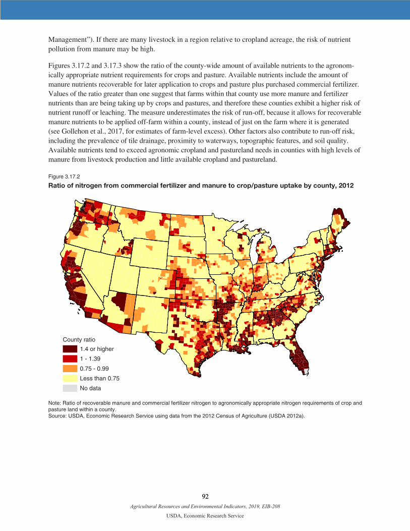
Agricultural Resources and Environmental Indicators, 2019, EIB-208
USDA, Economic Research Service
92 92
Management”). If there are many livestock in a region relative to cropland acreage, the risk of nutrient pollution from manure may be high.
Figures 3.17.2 and 3.17.3 show the ratio of the county-wide amount of available nutrients to the agronom-ically appropriate nutrient requirements for crops and pasture. Available nutrients include the amount of manure nutrients recoverable for later application to crops and pasture plus purchased commercial fertilizer. Values of the ratio greater than one suggest that farms within that county use more manure and fertilizer nutrients than are being taking up by crops and pastures, and therefore these counties exhibit a higher risk of nutrient runoff or leaching. The measure underestimates the risk of run-off, because it allows for recoverable manure nutrients to be applied off-farm within a county, instead of just on the farm where it is generated (see Gollehon et al., 2017, for estimates of farm-level excess). Other factors also contribute to run-off risk, including the prevalence of tile drainage, proximity to waterways, topographic features, and soil quality. Available nutrients tend to exceed agronomic cropland and pastureland needs in counties with high levels of manure from livestock production and little available cropland and pastureland.
Figure 3.17.2
Ratio of nitrogen from commercial fertilizer and manure to crop/pasture uptake by county, 2012
County ratio
1.4 or higher
1 - 1.39
0.75 - 0.99
Less than 0.75
No data
Note: Ratio of recoverable manure and commercial fertilizer nitrogen to agronomically appropriate nitrogen requirements of crop and pasture land within a county.Source: USDA, Economic Research Service using data from the 2012 Census of Agriculture (USDA 2012a).
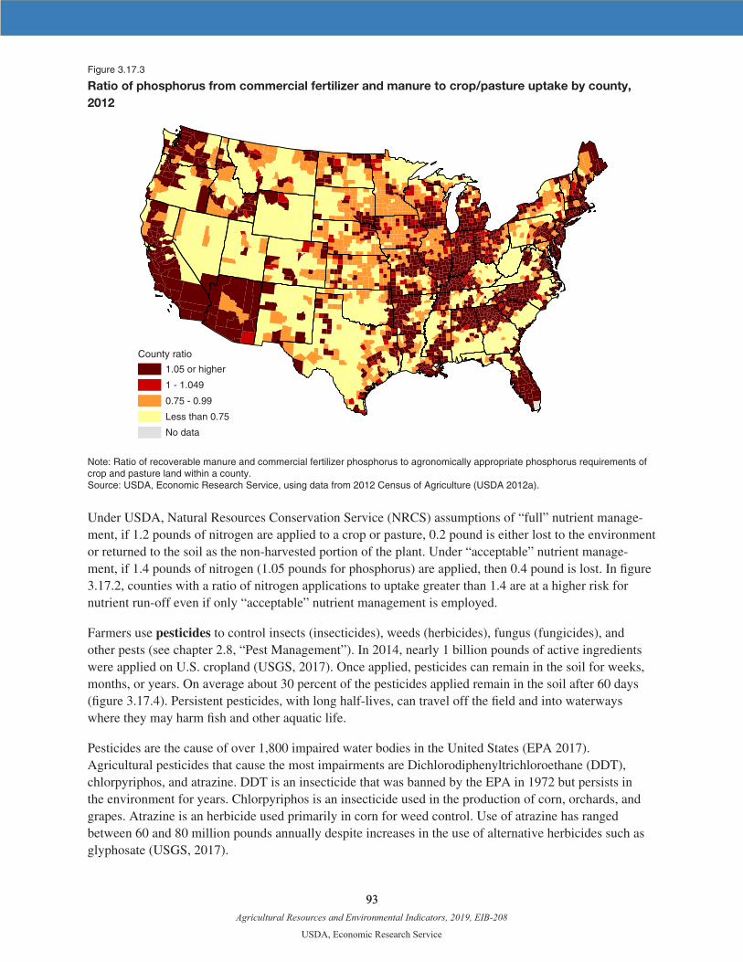
Agricultural Resources and Environmental Indicators, 2019, EIB-208
USDA, Economic Research Service
93 93
Figure 3.17.3
Ratio of phosphorus from commercial fertilizer and manure to crop/pasture uptake by county, 2012
County ratio
1.05 or higher
1 - 1.049
0.75 - 0.99
Less than 0.75
No data
Note: Ratio of recoverable manure and commercial fertilizer phosphorus to agronomically appropriate phosphorus requirements of crop and pasture land within a county.Source: USDA, Economic Research Service, using data from 2012 Census of Agriculture (USDA 2012a).
Under USDA, Natural Resources Conservation Service (NRCS) assumptions of “full” nutrient manage-ment, if 1.2 pounds of nitrogen are applied to a crop or pasture, 0.2 pound is either lost to the environment or returned to the soil as the non-harvested portion of the plant. Under “acceptable” nutrient manage-ment, if 1.4 pounds of nitrogen (1.05 pounds for phosphorus) are applied, then 0.4 pound is lost. In figure 3.17.2, counties with a ratio of nitrogen applications to uptake greater than 1.4 are at a higher risk for nutrient run-off even if only “acceptable” nutrient management is employed.
Farmers use pesticides to control insects (insecticides), weeds (herbicides), fungus (fungicides), and other pests (see chapter 2.8, “Pest Management”). In 2014, nearly 1 billion pounds of active ingredients were applied on U.S. cropland (USGS, 2017). Once applied, pesticides can remain in the soil for weeks, months, or years. On average about 30 percent of the pesticides applied remain in the soil after 60 days (figure 3.17.4). Persistent pesticides, with long half-lives, can travel off the field and into waterways where they may harm fish and other aquatic life.
Pesticides are the cause of over 1,800 impaired water bodies in the United States (EPA 2017). Agricultural pesticides that cause the most impairments are Dichlorodiphenyltrichloroethane (DDT), chlorpyriphos, and atrazine. DDT is an insecticide that was banned by the EPA in 1972 but persists in the environment for years. Chlorpyriphos is an insecticide used in the production of corn, orchards, and grapes. Atrazine is an herbicide used primarily in corn for weed control. Use of atrazine has ranged between 60 and 80 million pounds annually despite increases in the use of alternative herbicides such as glyphosate (USGS, 2017).
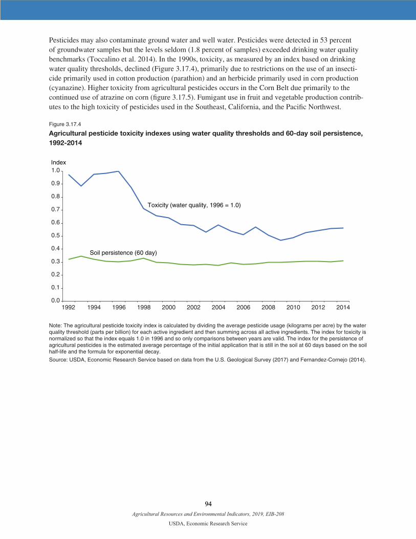
Agricultural Resources and Environmental Indicators, 2019, EIB-208
USDA, Economic Research Service
94 94
Pesticides may also contaminate ground water and well water. Pesticides were detected in 53 percent of groundwater samples but the levels seldom (1.8 percent of samples) exceeded drinking water quality benchmarks (Toccalino et al. 2014). In the 1990s, toxicity, as measured by an index based on drinking water quality thresholds, declined (Figure 3.17.4), primarily due to restrictions on the use of an insecti-cide primarily used in cotton production (parathion) and an herbicide primarily used in corn production (cyanazine). Higher toxicity from agricultural pesticides occurs in the Corn Belt due primarily to the continued use of atrazine on corn (figure 3.17.5). Fumigant use in fruit and vegetable production contrib-utes to the high toxicity of pesticides used in the Southeast, California, and the Pacific Northwest.
Figure 3.17.4
Agricultural pesticide toxicity indexes using water quality thresholds and 60-day soil persistence, 1992-2014
0.0
0.1
0.2
0.3
0.4
0.5
0.6
0.7
0.8
0.9
1.0
1992 1994 1996 1998 2000 2002 2004 2006 2008 2010 2012 2014
Soil persistence (60 day)
Toxicity (water quality, 1996 = 1.0)
Index
Note: The agricultural pesticide toxicity index is calculated by dividing the average pesticide usage (kilograms per acre) by the water quality threshold (parts per billion) for each active ingredient and then summing across all active ingredients. The index for toxicity is normalized so that the index equals 1.0 in 1996 and so only comparisons between years are valid. The index for the persistence of agricultural pesticides is the estimated average percentage of the initial application that is still in the soil at 60 days based on the soil half-life and the formula for exponential decay.
Source: USDA, Economic Research Service based on data from the U.S. Geological Survey (2017) and Fernandez-Cornejo (2014).
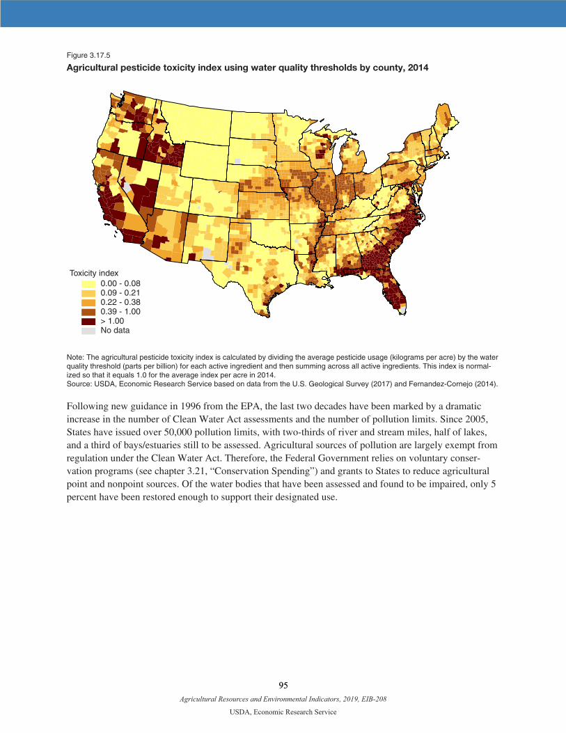
Agricultural Resources and Environmental Indicators, 2019, EIB-208
USDA, Economic Research Service
95 95
Figure 3.17.5
Agricultural pesticide toxicity index using water quality thresholds by county, 2014
Toxicity index 0.00 - 0.080.09 - 0.210.22 - 0.380.39 - 1.00> 1.00No data
Note: The agricultural pesticide toxicity index is calculated by dividing the average pesticide usage (kilograms per acre) by the water quality threshold (parts per billion) for each active ingredient and then summing across all active ingredients. This index is normal-ized so that it equals 1.0 for the average index per acre in 2014.Source: USDA, Economic Research Service based on data from the U.S. Geological Survey (2017) and Fernandez-Cornejo (2014).
Following new guidance in 1996 from the EPA, the last two decades have been marked by a dramatic increase in the number of Clean Water Act assessments and the number of pollution limits. Since 2005, States have issued over 50,000 pollution limits, with two-thirds of river and stream miles, half of lakes, and a third of bays/estuaries still to be assessed. Agricultural sources of pollution are largely exempt from regulation under the Clean Water Act. Therefore, the Federal Government relies on voluntary conser-vation programs (see chapter 3.21, “Conservation Spending”) and grants to States to reduce agricultural point and nonpoint sources. Of the water bodies that have been assessed and found to be impaired, only 5 percent have been restored enough to support their designated use.

Agricultural Resources and Environmental Indicators, 2019, EIB-208
USDA, Economic Research Service
96 96
References
Argabright, M.S., R.G. Cronshey, J.D. Helms, G.A. Pavelis, and H.R. Sinclair. 1996. Historical Changes in Soil Erosion, 1930-1992: the Northern Mississippi Valley Loess Hills. Historical Notes Number 5. U.S. Department of Agriculture, Natural Resources Conservation Service. Resource Economics and Social Sciences Division.
Belmont, P., K.B. Gran, S.P. Schottler, P.R. Wilcock, S.S. Day, C. Jennings, J.W. Lauer, E. Viparelli, J.K. Willenbring, D.R. Engstrom, and G. Parker. 2011. “Large shift in source of fine sediment in the upper Mississippi River,” Environmental Science & Technology 45.
Dubrovsky, N.M., K.R. Burow, G.M. Clark, J.M. Gronberg, P.A. Hamilton, K.J. Hitt, D.K. Mueller, M.D. Munn, B.T. Nolan, L.J. Puckett, M.G. Rupert, T.M. Short, N.E. Spahr, L.A. Sprague, and W.G. Wilber. 2010. The quality of our Nation’s waters—Nutrients in the Nation’s streams and groundwater, 1992-2004. U.S. Geological Survey Circular 1350.
Fernandez-Cornejo, J., R. Nehring, C. Osteen, S. Wechsler, A. Martin, and A. Vialou. 2014. Pesticide Use in U.S. Agriculture: 21 Selected Crops, 1960-2008. EIB-124, U.S. Department of Agriculture, Eco-nomic Research Service, May.
Gollehon, N., R. Kellogg, D. Moffitt. 2017. Estimates of Recoverable and Non-Recoverable Manure Nutrients Based on the Census of Agriculture—2012 Results. Washington DC: U.S. Department of Agriculture, June.
Schottler, S.P., J. Ulrich, P. Belmont, R. Moore, J. Lauer, D.R. Engstrom, and J.E. Almendinger. 2014. “Twentieth century agricultural drainage creates more erosive rivers,” Hydrological Processes 28.
Toccalino, P.L., R.J. Gilliom, B.D. Lindsey, and M.G. Rupert. 2014. “Pesticides in Groundwater of the United States: Decadal-Scale Changes, 1993-2011,” Groundwater 52. doi:10.1111/gwat.12176
U.S. Department of Agriculture. 2012a. Census of Agriculture, National Agricultural Statistic Service. U.S. Department of Agriculture 2012b. Natural Resources Conservation Service and Center for Survey
Statistics and Methodology, Iowa State University. National Resources Inventory.U.S. Environmental Protection Agency. 2017. Water Quality Assessment and TMDL Information. U.S. Geological Survey. 2017. Pesticide National Synthesis Project, National Water-Quality Assessment
(NAWQA) Project. Zaimes, G., R.C. Schultz, and T.M. Isenhart. 2006. “Riparian land uses and precipitation influences on
stream bank erosion in central Iowa,” Journal of the American Water Resources Association 42(1).

Agricultural Resources and Environmental Indicators, 2019, EIB-208
USDA, Economic Research Service
97 97
Chapter 3.18—Renewable Energy
Claudia Hitaj and Scott Malcolm
• From 2007 to 2012, the number of farms producing onfarm renewable energy more than doubled to 57,299 (2.7 percent of all farms).
• Ethanol production grew from 3.9 billion gallons in 2005 to 15.8 billion gallons in 2017.
• In the 2016-17 marketing year, about 37 percent of corn production was used as a feedstock for eth-anol production, and about 27 percent of soybean production was allocated to biodiesel production.
Since the early 2000s, farmers have increased renewable energy production in response to cost and tech-nology improvements, as well as Government incentives for renewable energy and the Renewable Fuel Standard (RFS), which mandates the use of biofuels in transportation. Onfarm energy-generation technol-ogies include wind power, solar power, small hydropower, methane digesters, and geothermal exchange. Farmers can also produce renewable power indirectly by growing biomass feedstocks, leasing land for utility-scale solar power installations, or leasing their wind rights and hosting utility-scale wind turbines.
Some of the renewable power produced on farms is for the farm’s own consumption only—such as for solar-powered electric fences or water pumps for watering livestock in remote areas—and is not grid-con-nected. Farmers can also connect their renewable power systems to the grid, receiving a credit for part of the electricity generated and selling any excess electricity to the grid. At the other extreme, the renewable power produced may go exclusively to the grid, as in the case of utility-scale wind turbines that are part of a larger wind power plant facility potentially covering multiple farms.
Onfarm Renewable Power Production Varies Regionally
In 2007, 23,451 U.S. farms (1.1 percent of all U.S. farms) produced energy onfarm with solar panels, geothermal exchange, wind turbines, small hydro, or methane digesters (USDA-NASS, 2014). By 2012, farms producing renewable energy had more than doubled to 57,299 (2.7 percent of farms) (fig. 3.18.1).
Among U.S. farm businesses,1 adoption of onfarm renewable energy systems is concentrated in the Western States, Illinois, and New England (fig. 3.18.2) and is correlated with State policies that support renewable energy, such as Renewable Portfolio Standards (mandates for renewable electricity) and production tax credits. Adoption rates are low in the Southeast.
1USDA defines a farm as any place that produced and sold or normally would have produced and sold at least $1,000 of agricultural products during a given year. Farm businesses include only farms where the primary operator is currently employed and spends the majority of work time on agricultural production, or, if the primary operator is largely employed off-farm, the operation has over $350,000 in annual gross cash farm income.

Agricultural Resources and Environmental Indicators, 2019, EIB-208
USDA, Economic Research Service
98 98
Figure 3.18.1
Number of agricultural operations with onfarm renewable energy producing systems, by type of system, 2012
0 5,000 10,000 15,000 20,000 25,000 30,000 35,000 40,000
Solar panels
Geoexchange
Wind turbines
Biodiesel
Ethanol
Small hydro
Other
Methane digesters
Note: Ethanol and biodiesel refer to farms producing these biofuels directly for consumption by the operation and do not refer to farms growing feedstocks, such as corn and soybeans, used to produce biofuels. Source: USDA, Economic Research Service using data from the 2012 Census of Agriculture (USDA, NASS, 2014).
Figure 3.18.2
Share of farm businesses with onfarm renewable energy (RE) systems by county, 2012
Percent
01 - 56 - 1011 - 2021 - 45
Source: USDA, Economic Research Service using data from the 2012 Census of Agriculture (USDA, NASS, 2014).

Agricultural Resources and Environmental Indicators, 2019, EIB-208
USDA, Economic Research Service
99 99
The capacity of renewable energy systems installed onfarm is, on average, less than 100 kilowatts (kW) for wind and 4.4 kW for solar (Xiarchos and Vick, 2011). However, a small wind system of 100 kW can generate 840 kilowatt hours (kWh) in a day (assuming a 35-percent capacity factor), meeting a substantial share of electricity consumption on most operations. In 2014, electricity consumption on farms ranged from about 1,110 kWh per day for peanut farms to 806 kWh per day for dairy farms, 250 kWh per day for corn farms, and 150 kWh per day for wheat farms.2
Solar Power
In agriculture, solar energy can be used in a solar thermal system or in a photovoltaic (PV) system to convert solar radiation to electricity. Solar energy generated on farms is used to power electric fencing, lighting, water pumps, pond aeration, and ventilation. Farmers can take advantage of the Federal invest-ment tax credit, which amounts to 30 percent of expenditures to install a solar system after the exclusion of any subsidized portion of the project.
Wind Power
In 2012, wind turbines could be found on 9,054 U.S. farms. Most turbines are owned by energy compa-nies who lease the wind rights from the farm landowners. A 2009 survey, which limited the response to wind turbines owned by the farm operation, showed that only 1,420 U.S. farms (0.06 percent of opera-tions) owned wind turbines, and the majority of these turbines had a capacity of less than 100 kW (small-scale) (USDA-NASS, 2011). In contrast, utility-scale wind turbines have a capacity of 1,000 to 2,500 kW.
In 2014, farm operators who leased their wind rights earned on average $3,320 per year in lease income (table 3.18.1). Income from leasing oil and gas rights, such as for drilling oil or gas wells in shale plays, is much higher, averaging $57,000 in 2014 for the United States as a whole and about $157,000 in Pennsylvania (Marcellus shale) and North Dakota (Bakken shale) (Hitaj and Suttles, 2016).
Table 3.18.1
Income from leases associated with energy production for farms leasing wind rights, 2014 (select States)
Annual average wind-rights lease income per farm operation
United States $3,320
Iowa $4,120
Indiana $3,630
Illinois $3,620
Minnesota $2,680
Wisconsin $1,130
Texas $790
Source: USDA, Economic Research Service and National Agricultural Statistics Service, 2014 Tenure, Ownership, and Transition of Agricultural Land Survey.
2These calculations are based on the average expenses for electricity for farms by principal commodity from the ERS/NASS 2014 Agricultural Resource Management Survey, as well as the industrial retail rate of electricity of 7 cents per kWh from Energy Information Administration’s Electric Power Monthly February 2015 report. We use data from 2014 to be consistent with the next section, which relies on data from a 2014 survey.

Agricultural Resources and Environmental Indicators, 2019, EIB-208
USDA, Economic Research Service
100 100
Biofuel and Cellulosic Feedstock Production
Since 2005, the Renewable Fuel Standard and its supporting programs have contributed to a growing market for renewable transportation fuels. Ethanol production grew from 3.9 billion gallons in 2005 to 15.8 billion gallons in 2017 (EIA, 2018a). In the 2016-17 marketing year, about 37 percent of corn production was used as a feedstock for ethanol production, while about 27 percent of soybean produc-tion was allocated to biodiesel production (USDA-ERS, 2018). The biodiesel market is smaller than the ethanol market, and soybeans provide about half of biodiesel feedstocks. In 2017, 1.6 billion gallons of biodiesel were produced from soybeans (53 percent), animal fats (9 percent), corn oil (13 percent), and canola oil (12 percent), among other sources (EIA, 2018b). Biofuels are generally produced in commer-cial ethanol and biodiesel plants, though some farms (less than 0.3 percent of farms in 2012) produce biofuels directly on the operation: 4,099 farms produced biodiesel and 2,364 farms produced ethanol in 2012. Biodiesel and ethanol produced directly on farms can be for farm use or for outside sale.
Unlike ethanol and biodiesel, cellulosic biofuels are derived from nonfood biomass feedstocks, including crop residues, wood wastes, energy crops, and municipal solid wastes. Volumes of cellulosic biofuel production are small relative to corn ethanol production in the RFS, although cellulosic feedstocks can also be used for electricity production. Cellulosic biomass may have an advantage over conventional biofuels because its sources are either waste products or dedicated energy crops, such as switchgrass and miscanthus, which may be harvested from land not productive for food agriculture. Technological chal-lenges in producing biofuel from cellulosic feedstocks have resulted in annual reductions of the cellulosic biofuel mandate in the RFS since enactment of the Energy Independence and Security Act in 2007. The mandate was first exceeded in 2014 with production of 33 million gallons of cellulosic ethanol. In 2012, nearly 12,000 farms (0.5 percent) harvested cellulosic biomass, including crop residue, grasses, and woody biomass (and excluding grains, oilseeds, and wood), for use in the production of renewable energy (USDA-NASS, 2014).
Conclusion
Agricultural operations are uniquely suited for renewable energy production, as farms often require large amounts of electricity and feature ample space to house solar power installations or wind turbines. In other cases, nongrid-connected renewable power installations are the only way to economically power electric fences or water pumps in remote locations. As the economics of both utility-scale and distributed renewable power evolve, the rate of adoption of renewable power on farms may continue to increase; the share of farms with renewable power installations more than doubled from 2007 to 2012.
Farms produce corn used in ethanol production as well as soybeans, canola, and animal fats used in biodiesel production. Increased acreage due to additional biofuel feedstock demand affects land manage-ment, with implications for soil productivity, water quality/quantity, air quality, and greenhouse gas (GHG) emissions. Because regions differ in how crop production translates to environmental outcomes, the effect on environmental indicators (e.g., soil erosion, nutrient runoff, and GHG emissions) varies considerably by region. In some regions, the changes in environmental measures are greater than the change in acreage, indicating an intensification of input use and, possibly, expanded production on marginal lands.
Technological advances in cellulosic biomass may induce more farmers to grow cellulosic feedstock, such as switchgrass, for the advanced biofuel market. This development would carry with it the benefit of reduced nutrient runoff, as native grasses, including switchgrass, have extensive root networks that reach deep into the soil and increase water filtration, nutrient holding capacity, and erosion control.
Agricultural Resources and Environmental Indicators, 2019, EIB-208
USDA, Economic Research Service
101 101
References
Hitaj, C., and S. Suttles. 2016. Trends in U.S. Agriculture’s Consumption and Production of Energy: Renewable Power, Shale Energy, and Cellulosic Biomass. EIB-159. U.S. Department of Agriculture, Economic Research Service.
U.S. Energy Information Administration, Department of Energy. 2018a. Monthly Energy Review: Fuel Ethanol Overview.
U.S. Energy Information Administration, Department of Energy. 2018b. Monthly Biodiesel Production Report.
U.S. Department of Agriculture, Economic Research Service. 2018. U.S. Bioenergy Statistics. U.S. Department of Agriculture, National Agricultural Statistics Service. 2011. “Onfarm Renewable Ener-
gy Production Survey (2009).” U.S. Department of Agriculture, National Agricultural Statistics Service. 2014. Census of Agriculture
(multiple years).Xiarchos, I.M., and B. Vick. 2011. Solar Energy Use in U.S. Agriculture: Overview and Policy Issues.
U.S. Department of Agriculture, Office of the Chief Economist.

Agricultural Resources and Environmental Indicators, 2019, EIB-208
USDA, Economic Research Service
102 102
Chapter 3.19—Soil Health
Maria Bowman, Lori Lynch, and Steven Wallander
• Farmers can use management practices, such as no-till and cover crops, to build soil health. Accord-ing to the 2012 Census of Agriculture, 35 percent of cropland acres were in no-till and 3 percent were planted with a cover crop.
• As farmers have adopted soil health and soil conservation practices, they have contributed to declin-ing rates of soil erosion. Between 1982 and 2012, erosion on cultivated cropland (due to water and wind) declined by 45 percent.
• USDA incentivizes farmers to adopt soil health practices through programs such as the Environ-mental Quality Incentives Program (EQIP) and the Conservation Stewardship Program (CSP). Be-tween 2006 and 2016, the number of acres receiving EQIP payments for cover cropping more than quadrupled. Between 2010 and 2015, the number of acres receiving CSP payments for at least one soil health practice or enhancement grew from just under 7 million to more than 30 million.
Soil health refers to “the continued capacity of soil to function as a vital living ecosystem that sustains plants, animals, and humans” (USDA Natural Resources Conservation Service, 2017a). Healthy soil can support crop or livestock production, while at the same time generating ecosystem services—such as reducing nutrient pollution to streams and rivers—that benefit society. Soil scientists have developed several indicators—soil organic carbon, soil aggregation, readily available carbon/nitrogen pools, and soil microbial activity/diversity—that reflect underlying soil processes to help assess the health of agricul-tural soils (NRCS, 2018b). Soil health is related to soil type and location, but can also be influenced by land use and management decisions made by farmers. One important indicator of soil health, soil organic carbon, varies greatly across the United States (fig. 3.19.1).
Figure 3.19.1
Soil organic carbon stocks in the United States, 2013
Estimated carbon stocks in top 100 centimeters(milligrams soil organic
carbon per hectare)
300.1 to 3,000150.1 to 300125.1 to 150100.1 to 12550.1 to 10025.1 to 501 to 25
Note: Soil organic matter is only shown for cropland. Source: USDA, Economic Research Service mapping based on data produced from “Soil Survey Staff and T. Loecke. 2016. Rapid Carbon Assessment: Methodology, Sampling, and Summary. S. Wills (ed.). USDA, Natural Resources Conservation Service.”

Agricultural Resources and Environmental Indicators, 2019, EIB-208
USDA, Economic Research Service
103 103
Selected Soil Health Management Practices
No-till: Growing crops without tilling (i.e., plowing) the soil
Reduced-till/mulch-till/conservation-till: Ways of tilling the soil that minimize disturbance to the soil or maintain more residue cover than conventional tillage
Mulching: Adding plant residue (or other materials) to the surface of the soil
Cover cropping: Growing a crop, often over the winter, that will be left in place as residue or incorpo-rated into the soil to increase organic matter
Conservation crop rotation: Choosing crop rotations to maximize crop diversity, build organic matter, and improve soil biodiversity
Nutrient management: Adjusting the type, location, rate, and timing of fertilizer or other nutrients to meet plant needs and minimize environmental impacts
Prescribed/rotational grazing: Managing where and when livestock graze in order to prevent over-grazing and to optimize pasture growth
Note: See USDA Natural Resources Conservation Service (2017a) for more information on soil health practices.Source: USDA, Economic Research Service, Bowman et al., 2016.
Many farmers and ranchers use practices that contribute to soil health, such as no-till or reduced tillage, cover cropping, nutrient management, and prescribed or rotational grazing of livestock (see box, “Selected Soil Health Management Practices”). These practices exemplify one or more key principles that contribute to soil health: keep the soil covered as much as possible, disturb the soil as little as possible, keep plants growing throughout the year to feed the soil, and diversify as much as possible using crop rotation and cover crops (USDA Natural Resources Conservation Service, 2017).
According to the 2012 Census of Agriculture, 35 percent of U.S. cropland acres were in no-till, and 3 percent were planted with a cover crop. Over 130,000 farms (9 percent of farms) planted a cover crop in 2012 (excluding Conservation Reserve Program acreage) for a total of 10,280,793 acres. Almost a quarter of the cover crop acreage nationally was planted on farms ranging in size from 200 to 499 acres; 22 percent was on farms with more than 1,000 acres. Though smaller farms made up a small share of the total acreage planted to cover crops, 70 percent of the operations that planted cover crops farmed fewer than 50 acres.
Some regions report using practices such as no-till and cover crops more frequently. For example, no-till/strip-till and cover cropping were more widely used in the Southeast in 2012 (fig. 3.19.2; Wade et al., 2015). Farmers manage their soil differently due to many factors, including topography and local weather patterns. Farmers with hilly or bare land may derive more benefits from implementing practices such as no-till because they decrease soil erosion and benefit crop production. Fields with high erosion indexes may also be required to implement such practices as part of “conservation compliance” in order to be eligible to receive farm program benefits (Claassen et al., 2017). Cover cropping may be more common in the Southeast due to greater relative benefits from weed control or from cover cropping on ultisol soils that suffer from poor soil texture/structure and low organic matter (Duzy, 2017). It may also be easier to establish and terminate a winter cover crop in the Southeast, which has a longer growing season than most other regions (see chapter 2.12, “Crop Production Management: Tillage Practices”).
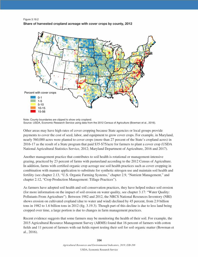
Agricultural Resources and Environmental Indicators, 2019, EIB-208
USDA, Economic Research Service
104 104
Figure 3.19.2
Share of harvested cropland acreage with cover crops by county, 2012
Percent with cover crops
0-1 1-5 5-10 10-1515-56
Note: County boundaries are clipped to show only cropland.Source: USDA, Economic Research Service using data from the 2012 Census of Agriculture (Bowman et al., 2016).
Other areas may have high rates of cover cropping because State agencies or local groups provide payments to cover the cost of seed, labor, and equipment to grow cover crops. For example, in Maryland, nearly 560,000 acres were planted to cover crops (more than 27 percent of the State’s cropland acres) in 2016-17 as the result of a State program that paid $35-$75/acre for farmers to plant a cover crop (USDA National Agricultural Statistics Service, 2012; Maryland Department of Agriculture, 2016 and 2017).
Another management practice that contributes to soil health is rotational or management-intensive grazing, practiced by 23 percent of farms with pastureland according to the 2012 Census of Agriculture. In addition, farms with certified organic crop acreage use soil health practices such as cover cropping in combination with manure application to substitute for synthetic nitrogen use and maintain soil health and fertility (see chapter 2.13, “U.S. Organic Farming Systems,” chapter 2.9, “Nutrient Management,” and chapter 2.12, “Crop Production Management: Tillage Practices”).
As farmers have adopted soil health and soil conservation practices, they have helped reduce soil erosion (for more information on the impact of soil erosion on water quality, see chapter 3.17: “Water Quality: Pollutants From Agriculture”). Between 1982 and 2012, the NRCS National Resources Inventory (NRI) shows erosion on cultivated cropland (due to water and wind) declined by 45 percent, from 2.9 billion tons in 1982 to 1.6 billion tons in 2012 (fig. 3.19.3). Though part of this decline is due to less land being cropped over time, a large portion is due to changes in farm management practices.
Recent evidence suggests that some farmers may be monitoring the health of their soil. For example, the 2015 Agricultural Resource Management Survey (ARMS) found that 16 percent of farmers with cotton fields and 11 percent of farmers with oat fields report testing their soil for soil organic matter (Bowman et al., 2016).
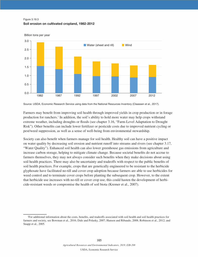
Agricultural Resources and Environmental Indicators, 2019, EIB-208
USDA, Economic Research Service
105 105
Figure 3.19.3
Soil erosion on cultivated cropland, 1982-2012
Billion tons per year
0.0
0.5
1.0
1.5
2.0
2.5
3.0
1982 1987 1992 1997 2002 2007 2012
Water (sheet and rill) Wind
Source: USDA, Economic Research Service using data from the National Resources Inventory (Claassen et al., 2017).
Farmers may benefit from improving soil health through improved yields in crop production or in forage production for ranchers.1 In addition, the soil’s ability to hold more water may help crops withstand extreme weather, including droughts or floods (see chapter 3.16, “Farm-Level Adaptation to Drought Risk”). Other benefits can include lower fertilizer or pesticide costs due to improved nutrient cycling or pest/weed suppression, as well as a sense of well-being from environmental stewardship.
Society can also benefit when farmers manage for soil health. Healthy soil can have a positive impact on water quality by decreasing soil erosion and nutrient runoff into streams and rivers (see chapter 3.17, “Water Quality”). Enhanced soil health can also lower greenhouse gas emissions from agriculture and increase carbon storage, helping to mitigate climate change. Because societal benefits do not accrue to farmers themselves, they may not always consider such benefits when they make decisions about using soil health practices. There may also be uncertainty and tradeoffs with respect to the public benefits of soil health practices. For example, crops that are genetically engineered to be resistant to the herbicide glyphosate have facilitated no-till and cover crop adoption because farmers are able to use herbicides for weed control and to terminate cover crops before planting the subsequent crop. However, to the extent that herbicide use increases with no-till or cover crop use, this could hasten the development of herbi-cide-resistant weeds or compromise the health of soil biota (Kremer et al., 2007).
1For additional information about the costs, benefits, and tradeoffs associated with soil health and soil health practices for farmers and society, see Bowman et al., 2016; Dale and Polasky, 2007; Hansen and Ribaudo, 2008; Robinson et al., 2012; and Snapp et al., 2005.

Agricultural Resources and Environmental Indicators, 2019, EIB-208
USDA, Economic Research Service
106 106
Although farmers may benefit from improved soil health, additional costs of using soil health practices include buying seed to plant a cover crop, which farmers receive no revenue from since it is not harvested or sold. In addition, benefits from soil health practices may take years to realize. For these reasons and others, Federal and State programs may subsidize the cost of soil health practices that otherwise might be foregone by farmers.
USDA’s Natural Resources Conservation Service (NRCS) administers two programs that provide finan-cial assistance to farmers to retain or use soil health practices and enhancements: the Environmental Quality Incentives Program (EQIP)2 and the Conservation Stewardship Program (CSP).3 Farmers receive payments to implement or maintain practices like nutrient management, no-till, cover cropping, and pasture/rangeland management and restoration (see chapter 3.24, “Working-Lands Conservation Programs”). EQIP’s budget has increased since 1997 as it grants more contracts to eligible producers. EQIP expenditures on nutrient management and terracing have decreased, while expenditures on cover crops have increased (fig. 3.19.4).
Figure 3.19.4
Top five crop management practices (in terms of expenditures) in the Environmental Quality Incentives Program (EQIP), 1998-2015
Percent of payments
Residue management, no-till and strip till
Terraces
Nutrient managementCover crop
Conservation crop rotation
0
10
20
30
40
50
60
70
80
90
100
1998 99 00 01 02 03 04 05 06 07 08 09 10 11 12 13 14 15 16
Note: See box “Selected Soil Health Management Practices” for definitions of practices. Terraces are a structural practice designed to reduce runoff and soil erosion by constructing an earth embankment or ridge that is perpendicular to a field’s slope. Between 1998 and 2015, the total EQIP budget expanded from $19 million to $800 million.Source: USDA, Economic Research Service using data from USDA, Natural Resources Conservation Service, EQIP practice suite payments in the United States.
2EQIP provides payments up to 75 percent of the incurred costs and income foregone of certain conservation practices and activities (USDA Natural Resources Conservation Service, 2017c).
3CSP provides payment to maintain existing conservation activities, add additional activities, and to adopt a resource-conserving crop rotation (USDA Natural Resources Conservation Service, 2017d).

Agricultural Resources and Environmental Indicators, 2019, EIB-208
USDA, Economic Research Service
107 107
Between 2006 and 2016, the number of acres that received EQIP payments for cover cropping more than quadrupled (from 240,418 to 1,120,311), while annual spending on cover crops increased more than tenfold. Between 2010 and 2015, the number of acres receiving CSP payments for at least one soil health practice or enhancement grew from just under 7 million to more than 30 million (fig. 3.19.5).
Figure 3.19.5
Acres enrolled in the Conservation Stewardship Program (CSP) with at least one soil health practice or enhancement, 2010-15
Million acres
0
5
10
15
20
25
30
35
2010 2011 2012 2013 2014 2015
Note: These data include only active and completed contracts. For contracts that included more than one land unit and/or more than one soil health practice or enhancement (of the 100 practices or enhancements we considered to be related to soil health), we used the maximum value of the planned acres for each land unit that had at least one soil health practice/enhancement applied (to avoid double counting).Source: USDA, Economic Research Service calculations using USDA, Natural Resources Conservation Service, ProTracts database.

Agricultural Resources and Environmental Indicators, 2019, EIB-208
USDA, Economic Research Service
108 108
References
Bowman, M., S. Wallander, and L. Lynch. 2016. “An Economic Perspective on Soil Health,” Amber Waves Sept.
Claassen, R., M. Bowman, V. Breneman, T. Wade, R. Williams, J. Fooks, L. Hansen, R. Lovanna, and C. Loesch. 2017. Conservation Compliance: How Farmer Incentives Are Changing in the Crop Insurance Era. ERR-234. U.S. Department of Agriculture, Economic Research Service, July.
Dale, Virginia H., and Stephen Polasky. 2007. “Measures of the effects of agricultural practices on ecosys-tem services,” Ecological Economics 64(2).
Duzy, L. 2017. “Addressing Barriers to Conservation Systems Adoption Through Research.” C-FARE and USDA Economists webinar, June 27.
Hansen, L., and M. Ribaudo. 2008. Economic Measures of Soil Conservation Benefits: Regional Values for Policy Assessment. TB-1922. U.S. Department of Agriculture, Economic Research Service.
Kremer, R., N. Means, and S. Kim. 2007. “Glyphosate affects soybean root exudation and rhizosphere micro-organisms,” International Journal of Environmental Analytical Chemistry 85:15.
Maryland Department of Agriculture. 2016. “Maryland’s 2016-2017 Cover Crop Sign-up.” Maryland Department of Agriculture. 2017. “Maryland Farmers Break Cover Crop Planting Record…
Again.” Press Release, April 20. Robinson, D.A.; N. Hockley, E.Dominati, I. Lebron, K.M. Scow, B. Reynolds, B.A. Emmett, A.M. Keith,
L.W. de Jonge, P. Schjonning, P. Moldrup, S.B. Jones, and M. Tuller. 2012. “Natural capital, ecosys-tem services, and soil change: why soil science must embrace an ecosystems approach,” Vadose Zone Journal 11(1).
Snapp, S.S., S.M. Swinton, R. Labarta, D. Mutch, J.R. Black, R. Leep, J. Nyiraneza, and K. O’Neil. 2005. “Evaluating cover crops for benefits, costs and performance within cropping system niches,” Agronomy Journal 97(1).
U.S. Department of Agriculture, National Agricultural Statistics Service. 2012. 2012 Census of Agricul-ture—State Data, Maryland. Accessed from USDA NASS Quickstats.
U.S. Department of Agriculture, Natural Resources Conservation Service. 2017a. “Soil Health” page on NRCS Website.
U.S. Department of Agriculture, Natural Resources Conservation Service. 2017b. “Healthy, productive soils checklist for growers” page on NRCS Website.
U.S. Department of Agriculture, Natural Resources Conservation Service. 2017c. Environmental Quality Incentives Program page on NRCS Website.
U.S. Department of Agriculture, Natural Resources Conservation Service. 2017d. CSP Payments page on NRCS Website.
U.S. Department of Agriculture, Natural Resources Conservation Service. 2013. Soil Health Key Points document on NRCS Website.
Wade, Tara, Roger Claassen, and Steven Wallander. 2015. Conservation-Practice Adoption Rates Vary Widely by Crop and Region. EIB-147. U.S. Department of Agriculture, Economic Research Service.
Agricultural Resources and Environmental Indicators, 2019, EIB-208
USDA, Economic Research Service
109 109
Chapter 3.20—Pollinators: Honey Bee Status and Trends
Daniel Hellerstein, Claudia Hitaj, and David Smith
• Of the 2.7 million honey bee colonies in the United States in 2017, 87 percent were managed commercially.
• Since the early 2000s, annual honey bee colony loss has fluctuated between 30 and 45 percent, versus a historical average of 15 percent.
• Almost half (44 percent) of honey bee colonies spend summer in the Northern Plains States of Montana, North and South Dakota, and Minnesota, where forage resources declined between 2002 and 2012.
About one-third of the world’s food crops depend on insect pollinators—including managed honey bees and more than 4,000 species of native bees and other insects (USDA-NRCS, 2017). Some crops, such as almonds and melons, require insect pollination to produce nuts or fruit; others, such as tomatoes and apples, receive a yield boost from insect pollination.
Production of pollinated crops increased rapidly in the past decade. Between 2007 and 2016, the produc-tion value of almonds grew by 85 percent in real terms, while the production value of both apples and blueberries grew by about 15 percent. Estimates of the economic value provided by pollinators vary widely, with low estimates (in the hundreds of millions of dollars) considering only direct payments to beekeepers and higher estimates (as high as $19 billion) considering the maximum potential for lost agricultural production absent honey bees. An intermediate value of $15 billion is often cited (Pollinator Health Task Force, 2016).1
Of 2.7 million honey bee colonies in the United States in 2017 (USDA-NASS, 2018), about 87 percent were managed commercially by beekeepers with more than 500 colonies (Bee Informed Partnership, 2015). Honey bees provide an estimated 80 percent of pollination services (by value), with the rest provided by wild bees and other native pollinators (Losey and Vaughn, 2006). U.S. honey production from these colonies amounted to $336 million in 2016, along with $149 million in earnings from other products (including queen bees and beeswax) and $353 million from pollination services.
Honey bees and other pollinators face a variety of stressors, including diseases, insect pests, nutritional deficiencies, pesticide exposure, and changing landscapes. These factors, which can have synergistic effects, can affect the productivity and survival of pollinators. Honey bee colony numbers peaked at 5.9 million in 1947. After declining to 2.3 million colonies in 2008, colony numbers have since increased to 2.7 million by 2016/2017 (fig. 3.20.1). Despite a net increase in the number of managed honey bee colonies, annual losses of honey bee colonies have spiked over the last decade. Between 2006 and 2007, some 30 percent of honey bee colonies were lost during the overwinter period (October 1 through April 1), compared to a historical rate of 15 percent (Burgett et al., 2010). Though the overwinter loss rate has since diminished (21 percent in 2016-17), summertime losses have grown. The net result is that annual colony loss between 2012-17 averaged 40 percent, compared with 36 percent in 2010-11.
1The variation in estimates of the economic value of pollinators is largely driven by assumptions about producer adaptation. Higher values assume no adaptation, hence they represent an upper bound on the losses should pollinators disappear.

Agricultural Resources and Environmental Indicators, 2019, EIB-208
USDA, Economic Research Service
110 110
Figure 3.20.1
Managed U.S. honey bee colony numbers and loss estimates, 2006-17
Losses (percent)
1.8
1.9
2.0
2.1
2.2
2.3
2.4
2.5
2.6
2.7
2.8
0
5
10
15
20
25
30
35
40
45
50
2006-07 2007-08 2008-09 2009-10 2010-11 2011-12 2012-13 2013-14 2014-15 2015-16 2016-17
Total winter loss Total annual loss Number of colonies
Number of honey-producing colonies (millions)
Note: Annual colony loss estimates from the Bee Informed Partnership are for the period from October 1 to September 30 of the following year; winter loss estimates are for October 1 to April 1 of the following year. Before 2010-11, data on summer losses were not gathered. The data on the number of honey-producing colonies are from NASS Honey Report. Source: USDA, Economic Research Service using data from the Bee Informed Partnership (2017) and from USDA, National Agricultural Statistics Service, Honey Report (USDA-NASS, 2018).
The increase in colony numbers since 2008, even as colony mortality remains high, is due to beekeeper management, such as splitting colonies and the purchase of “packages” (small honey bee colonies containing a queen and a few thousand bees). By monitoring for pests and pathogens to inform the application of miti-cides, antibiotics, and other chemicals, and by providing supplemental feeds, intensified management can reduce colony losses. All of this management may result in increased costs to beekeepers.
While both wild bees and managed honey bees contribute to agricultural production, they in turn depend on forage resources—the pollen and nectar of flowering plants that bees feed on to survive. The quality and quantity of forage resources available to pollinators depends on land use and land cover (LULC). Shortening the distance between crop fields and natural habitat can enhance pollination by wild pollina-tors. A particular plot of land’s impacts on honey bee health may be less pronounced than on the health of native pollinators, both because honey bees cover a larger landscape (over 2 miles) to meet their nutri-tional requirements and because hives can be relocated by beekeepers.
A potential cause of increased honey bee losses could be a nationwide trend toward land uses and land covers that provide less forage for bees. Using 30 years of land-use data derived from the National Resources Inventory conducted by USDA’s Natural Resources Conservation Service, a honey bee forage suitability index (FSI) was constructed that aggregates LULC changes into a single measure of pollinator forage quality (Hellerstein et al., 2017)—with higher values indicating more favorable pollinator habitat. For example, grain crops (e.g., corn, wheat, rice, and barley) have low FSI scores of 0.16-0.17; most fruits and vegetables have FSI scores of 0.31-0.35; and pasture, forest, and grasslands have FSI scores of 0.45-0.48.
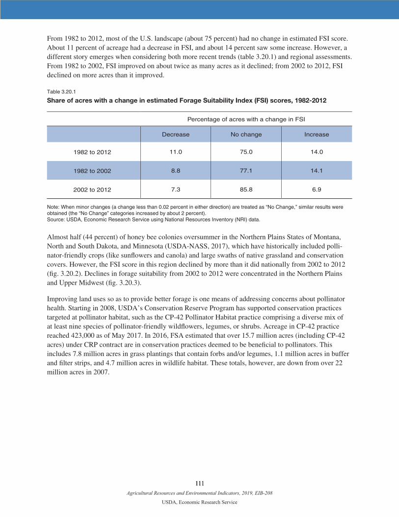
Agricultural Resources and Environmental Indicators, 2019, EIB-208
USDA, Economic Research Service
111 111
From 1982 to 2012, most of the U.S. landscape (about 75 percent) had no change in estimated FSI score. About 11 percent of acreage had a decrease in FSI, and about 14 percent saw some increase. However, a different story emerges when considering both more recent trends (table 3.20.1) and regional assessments. From 1982 to 2002, FSI improved on about twice as many acres as it declined; from 2002 to 2012, FSI declined on more acres than it improved.
Table 3.20.1
Share of acres with a change in estimated Forage Suitability Index (FSI) scores, 1982-2012
Percentage of acres with a change in FSI
Decrease No change Increase
1982 to 2012 11.0 75.0 14.0
1982 to 2002 8.8 77.1 14.1
2002 to 2012 7.3 85.8 6.9
Note: When minor changes (a change less than 0.02 percent in either direction) are treated as “No Change,” similar results were obtained (the “No Change” categories increased by about 2 percent).Source: USDA, Economic Research Service using National Resources Inventory (NRI) data.
Almost half (44 percent) of honey bee colonies oversummer in the Northern Plains States of Montana, North and South Dakota, and Minnesota (USDA-NASS, 2017), which have historically included polli-nator-friendly crops (like sunflowers and canola) and large swaths of native grassland and conservation covers. However, the FSI score in this region declined by more than it did nationally from 2002 to 2012 (fig. 3.20.2). Declines in forage suitability from 2002 to 2012 were concentrated in the Northern Plains and Upper Midwest (fig. 3.20.3).
Improving land uses so as to provide better forage is one means of addressing concerns about pollinator health. Starting in 2008, USDA’s Conservation Reserve Program has supported conservation practices targeted at pollinator habitat, such as the CP-42 Pollinator Habitat practice comprising a diverse mix of at least nine species of pollinator-friendly wildflowers, legumes, or shrubs. Acreage in CP-42 practice reached 423,000 as of May 2017. In 2016, FSA estimated that over 15.7 million acres (including CP-42 acres) under CRP contract are in conservation practices deemed to be beneficial to pollinators. This includes 7.8 million acres in grass plantings that contain forbs and/or legumes, 1.1 million acres in buffer and filter strips, and 4.7 million acres in wildlife habitat. These totals, however, are down from over 22 million acres in 2007.
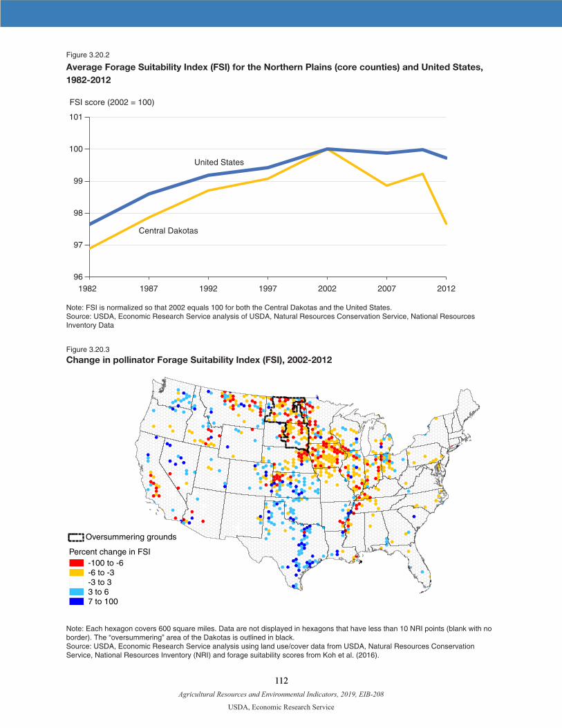
Agricultural Resources and Environmental Indicators, 2019, EIB-208
USDA, Economic Research Service
112 112
Figure 3.20.2
Average Forage Suitability Index (FSI) for the Northern Plains (core counties) and United States, 1982-2012
FSI score (2002 = 100)
96
97
98
99
100
101
1982 1987 1992 1997 2002 2007 2012
Central Dakotas
United States
Note: FSI is normalized so that 2002 equals 100 for both the Central Dakotas and the United States.Source: USDA, Economic Research Service analysis of USDA, Natural Resources Conservation Service, National Resources Inventory Data
Figure 3.20.3
Change in pollinator Forage Suitability Index (FSI), 2002-2012
Oversummering grounds
Percent change in FSI-100 to -6-6 to -3-3 to 33 to 67 to 100
Note: Each hexagon covers 600 square miles. Data are not displayed in hexagons that have less than 10 NRI points (blank with no border). The “oversummering” area of the Dakotas is outlined in black.Source: USDA, Economic Research Service analysis using land use/cover data from USDA, Natural Resources Conservation Service, National Resources Inventory (NRI) and forage suitability scores from Koh et al. (2016).
Agricultural Resources and Environmental Indicators, 2019, EIB-208
USDA, Economic Research Service
113 113
References
Bee Informed Partnership. 2017. A National Survey of Managed Honey Bee 2016-2017 Annual Colony Losses in the USA.
Burgett, M., S. Daberkow, R. Rucker, and W. Thurman. 2010. “U.S. Pollination Markets: Recent Changes and Historical Perspective,” American Bee Journal 150(1).
Hellerstein, D., C. Hitaj, D.J. Smith, and A. Davis. 2017. Land Use, Land Cover, and Pollinator Health: A Review and Trend Analysis. ERR-232, U.S. Department of Agriculture, Economic Research Service.
Koh, I., E.V. Lonsdorf, N.M. Williams, C. Brittain, R. Isaacs, J. Gibbs, and T.H. Ricketts. 2016. “Model-ing the Status, Trends, and Impacts of Wild Bee Abundance in the United States,” Proceedings of the National Academy of Sciences 113(1). doi: 10.1073/pnas.1517685113.
Losey, J.E., and M. Vaughan. 2006. “The Economic Value of Ecological Services Provided by Insects,” BioScience 56(4). doi: 10.1641/0006-3568(2006)56[311:tevoes]2.0.co;2.
Pollinator Health Task Force (2016). “Pollinator Partnership Action Plan.” U.S. Department of Agriculture and U.S. Environmental Protection Agency.
U.S. Government Accountability Office. 2016. BEE HEALTH: USDA and EPA Should Take Additional Actions to Address Threats to Bee Populations. GAO Report GAO-16-220., Feb.
U.S. Department of Agriculture, National Agricultural Statistics Service. 2018. Honey Report (multiple years).
U.S. Department of Agriculture, National Agricultural Statistics Service. 2017. Honey Bee Colonies Re-port.
U.S. Department of Agriculture, Natural Resources Conservation Service. 2017. Insects and Pollinators: Pollinators by the Numbers.

Agricultural Resources and Environmental Indicators, 2019, EIB-208
USDA, Economic Research Service
114 114
Chapter 3.21—Conservation Spending Seeks To Improve Environmental Performance in Agriculture
Roger Claassen
• Conservation programs provide financial and technical assistance to support the adoption of conser-vation practices on U.S. farms.
• After significant increases in conservation program spending under the 2002 and 2008 Farm Acts, funding leveled off under the 2014 Act.
• The shift in funding from land retirement to working land programs, begun under the 2002 Farm Act, continues.
Note: This chapter was prepared before the Agriculture Improvement Act of 2018 became law. For an update on conservation programs and conservation program spending, please see Agriculture Improvement Act of 2018: Highlights and Implications on the Economic Research Service website.
Some farming practices can degrade natural resources and the environment. Sediment, nutrient, and pesticide runoff and leaching, for example, can impair water quality (see chapter 3.17, “Water Quality: Pollutants from Agriculture”). Other practices can provide environmental benefits through careful management of agricultural land. For example, enhancing wildlife habitat on agricultural land by providing nesting material for migratory birds can help increase wildlife populations. USDA’s conserva-tion programs help agricultural producers improve environmental factors like soil quality, water quality, air quality, wildlife habitat, and greenhouse gas emissions.
A Portfolio of Incentive Programs
The USDA conservation effort relies mainly on voluntary incentive programs. Voluntary incentive programs can avoid the inherent difficulties in regulating geographically diffuse and elusive (difficult to monitor) sources of pollution and can minimize economic harm to farmers by offering a range of incen-tives and assistance programs. The following programs account for more than 95 percent of all USDA conservation program spending.
The Conservation Reserve Program (CRP) generally provides 10- to 15-year contracts to remove land from agricultural production. The latest acreage cap under the 2014 Farm Act for this program is 24 million acres. Most of the land enrolled in the CRP was in crop production prior to CRP enrollment and is now planted to grass or trees. Historically, a large majority of CRP contracts enrolled whole fields or whole farms. Increasingly, however, CRP contracts fund high-priority, partial-field practices such as filter strips and grass waterways, rather than whole-field or whole-farm enrollments (see chapter 3.23, “Conservation Reserve Program”). Up to 2 million acres of the 24 million acre CRP cap can be used for a specific grasslands enrollment where each landowner agrees to keep the land in grazing use rather than tilling it for crop production or converting it to any other use.
The Agricultural Conservation Easement Program (ACEP) provides long-term or permanent ease-ments for preservation of wetlands and the protection of agricultural land (cropland, grazing land, etc.) from commercial or residential development.
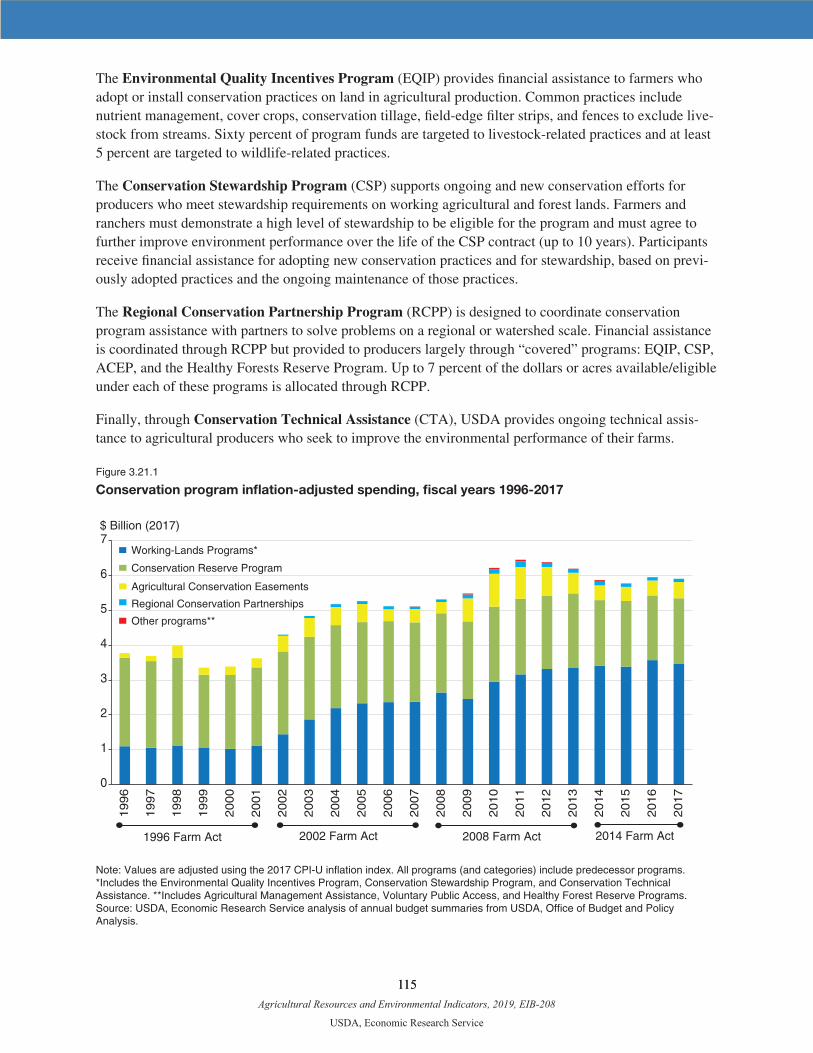
Agricultural Resources and Environmental Indicators, 2019, EIB-208
USDA, Economic Research Service
115 115
The Environmental Quality Incentives Program (EQIP) provides financial assistance to farmers who adopt or install conservation practices on land in agricultural production. Common practices include nutrient management, cover crops, conservation tillage, field-edge filter strips, and fences to exclude live-stock from streams. Sixty percent of program funds are targeted to livestock-related practices and at least 5 percent are targeted to wildlife-related practices.
The Conservation Stewardship Program (CSP) supports ongoing and new conservation efforts for producers who meet stewardship requirements on working agricultural and forest lands. Farmers and ranchers must demonstrate a high level of stewardship to be eligible for the program and must agree to further improve environment performance over the life of the CSP contract (up to 10 years). Participants receive financial assistance for adopting new conservation practices and for stewardship, based on previ-ously adopted practices and the ongoing maintenance of those practices.
The Regional Conservation Partnership Program (RCPP) is designed to coordinate conservation program assistance with partners to solve problems on a regional or watershed scale. Financial assistance is coordinated through RCPP but provided to producers largely through “covered” programs: EQIP, CSP, ACEP, and the Healthy Forests Reserve Program. Up to 7 percent of the dollars or acres available/eligible under each of these programs is allocated through RCPP.
Finally, through Conservation Technical Assistance (CTA), USDA provides ongoing technical assis-tance to agricultural producers who seek to improve the environmental performance of their farms.
Figure 3.21.1
Conservation program inflation-adjusted spending, fiscal years 1996-2017
$ Billion (2017)
0
1
2
3
4
5
6
7
1996
1997
1998
1999
2000
2001
2002
2003
2004
2005
2006
2007
2008
2009
2010
2011
2012
2013
2014
2015
2016
2017
Working-Lands Programs*
Conservation Reserve Program
Agricultural Conservation Easements
Regional Conservation Partnerships
Other programs**
1996 Farm Act 2002 Farm Act 2008 Farm Act 2014 Farm Act
Note: Values are adjusted using the 2017 CPI-U inflation index. All programs (and categories) include predecessor programs. *Includes the Environmental Quality Incentives Program, Conservation Stewardship Program, and Conservation Technical Assistance. **Includes Agricultural Management Assistance, Voluntary Public Access, and Healthy Forest Reserve Programs.Source: USDA, Economic Research Service analysis of annual budget summaries from USDA, Office of Budget and Policy Analysis.

Agricultural Resources and Environmental Indicators, 2019, EIB-208
USDA, Economic Research Service
116 116
Conservation Spending Declines Under the 2014 Farm Act
The Agricultural Act of 2014 (2014 Farm Act) consolidated USDA conservation programs, reducing the number from 23 to 13. The consolidated programs, however, retained most of the functions of conservation programs under the 2008 Farm Act. For example, the Agricultural Conservation Easement Program (ACEP) combines the functions of the Wetlands Reserve Program, the Farm and Ranchland Protection Program (FRPP), and the easement portion (60 percent) of the Grassland Reserve Program (GRP). ACEP funding, however, is significantly lower than under its three predecessor programs under the 2008 Farm Act.
After real growth in conservation spending under the 2002 and 2008 Farm Acts, (real) conservation funding was lower in fiscal year (FY)2014-FY2017 compared to FY2013, the last year under the 2008 Farm Act, or FY2011, the year of peak (real) spending under the 2008 Farm Act (fig. 3.21.1). The 2014 Farm Act continues to emphasize working land conservation, through funding for EQIP, CSP, and CTA. During 2012-17, combined funding for these programs was more than 50 percent of spending on major conservation programs. This emphasis reflects a long-term trend, begun under the 2002 Farm Act, that increased annual working land program spending from roughly $1 billion (in 2017 dollars) under the 1996 Act to more than $3 billion in fiscal years 2012-17 (see chapter 3.24, “Working-Lands Conservation Programs”).
Funding for temporary land retirement (through CRP) was steady for FY2014-FY2017 but was lower (in real terms) than at any time since 1996. CRP acreage declined in FY2014-FY2017, from 26.8 million acres at the end of FY2013 to 23.4 million acres at the end of FY2017. However, the average payment per enrolled acre rose from $61 at the end of FY2013 to $77 at the end of FY2017. The increased cost per acre reflects the increasing proportion of enrollment and higher rental rates for land in continuous signup. (Continuous signup focuses on high-priority conservation needs that generally command higher per-acre rental payments.) General signup acreage declined from 21.36 million acres to 16.02 million acres (-25 percent over 2013-17) while rental rates rose slightly from $49.90 per acre by $51.67 per acre (3.5 percent). Continuous signup acreage increased from 5.48 million acres to 7.33 million acres (33 percent) while the average rental rate rose from $103.48 per acre to $132.21 per acre (28 percent) (see chapter 3.23, “Conservation Reserve Program”).
Funding for long-term or permanent easements (through the Agricultural Conservation Easement Program (ACEP) and predecessor programs) has fallen in recent years. Real funding for easement programs peaked at roughly $920 million in fiscal year 2010 and has been roughly $400 million per year in fiscal years 2014-17.
Although direct funding for the Regional Conservation Partnership Program (RCPP) is limited to no more than $100 million per year, some funds from other conservation programs (e.g., EQIP) are directed to RCPP project cooperators, and RCPP partner groups also provide significant funding. During the first 3 years of the program (2014-16), $590 million in (nominal) USDA funding was directed to 200 projects (USDA-NRCS, 2016). Conservation partners provided $900 million (nominal) for both financial and technical assistance, resulting in a total of nearly $1.5 billion (nominal) in public and private funding for RCPP projects.
Agricultural Resources and Environmental Indicators, 2019, EIB-208
USDA, Economic Research Service
117 117
Conservation Compliance Ensures Consistency With Risk Management Programs
While conservation programs incentivize conservation on U.S. farms, Conservation Compliance ensures that other agricultural programs are also helping to achieve conservation goals. Since the 1930s, the Federal Government has set policies that support farm incomes in the event of low crop prices or crop failure. These policies also encourage farmers to conserve soil and, in more recent years, enhance environmental resources like water and air quality. By the 1980s, however, policymakers realized that farm support and conservation programs could work against each other. While conservation programs supported farmers in reducing soil erosion, for example, price and income support programs encouraged them to expand crop production onto environmentally sensitive lands, including erosion-prone land and wetlands. By linking farm program benefits to conservation, policymakers sought to limit these unin-tended consequences.
Conservation Compliance, first enacted as part of the 1985 Food Security Act, makes soil and wetland conservation a condition of eligibility for most Federal farm programs. Under Highly Erodible Land Conservation (HELC), farmers who grow crops on highly erodible land must apply an approved conservation system—one or more practices that work together to reduce soil erosion. Under Wetland Conservation (WC), farmers must refrain from draining wetland for crop production. Under the 2014 Farm Act, major programs subject to Conservation Compliance included farm commodity programs (e.g., Price Loss Coverage and Agriculture Risk Coverage), crop insurance premium subsidies, conservation program payments, and other agriculture-related payments.
References
Claassen, Roger, Maria Bowman, Vince Breneman, Tara Wade, Ryan Williams, Jacob Fooks, LeRoy Han-sen, Rich Iovanna, and Chuck Loesch. 2017. “Conservation Compliance in the Crop Insurance Era,” Amber Waves, U.S. Department of Agriculture, Economic Research Service, July.
U.S. Department of Agriculture, Natural Resources Conservation Service. 2016. RCPP: Partner-led Solu-tions, December.

Agricultural Resources and Environmental Indicators, 2019, EIB-208
USDA, Economic Research Service
118 118
Chapter 3.22—Wetlands: Status and Trends
LeRoy Hansen
• USDA attempts to discourage wetland conversions through Wetland Compliance; a 2017 analysis suggests that the program may be protecting about 75 percent of the wetland acreage in the Prairie Pothole Region.
• USDA improves and protects existing wetlands through the Conservation Reserve Program; as of July 2018, about 2.3 million acres were enrolled for wetlands protection.
• Since 2014, USDA has enrolled 229,000 acres for wetland restoration and protection through the Agricultural Conservation Easement Program.
Wetlands host unique, rich ecosystems critical to many plant and animal species. Over time, Federal support has shifted from funding wetland conversion to funding wetland restoration and protection.
Wetland Acreage
From 1992 through 2012, wetland acreage on non-Federal lands in the contiguous United States stayed at around 111 million (table 3.22.1). Having no net loss in wetland acreage for 20 years can be viewed as a conservation accomplishment because wetland losses (land converted to cropland or used for develop-ment) were the trend before 1992 (Hansen, 2006). Annual losses averaged around 850,000 acres between 1880 and 1954, 458,000 acres between 1954 and 1974, 290,000 acres between 1974 and 1982, and 79,000 acres between 1982 and 1992.
Table 3.22.1
From 1992-2012, total palustrine and estuarine wetland acreage showed no statistically significant change
Year Acres
1992 111.3
1997 111.1
2002 111.2
2007 111.3
2012 111.2
Note: The reported values are the acreage totals for each NRI survey year. The NRI is a statistical survey of natural resource conditions on non-Federal land in the United States including privately owned lands, Tribal and trust lands, and lands controlled by State and local governments.Source: USDA, Economic Research Service using data from USDA, Natural Resources Conservation Service (NRCS), 2015.
Agricultural Resources and Environmental Indicators, 2019, EIB-208
USDA, Economic Research Service
119 119
Over time, a natural back-and-forth shift between dryland and wetland habitat results in variations in wetland acreage. Natural shifts occur, for example, when changes in groundwater levels turn dryland to wetland, or vice versa. Between 1992 and 2012, about 1.5 million wetland acres became dryland and some other type of aquatic habitat, while about 1.6 million dryland and non-wetland aquatic habitat acres became wetland (table 25 in USDA, NRCS (2015)). Human activities also play a role. For example, the Natural Resources Conservation Service (NRCS) reported that between 1997 and 2007, about 266,000 wetland acres were lost through land development (table 15 in USDA, NRCS (2013)).
USDA Wetland Conservation Efforts
USDA protects wetlands through Wetland Compliance (WC), the Conservation Reserve Program (CRP), the Wetlands Reserve Program (WRP), and the Agricultural Conservation Easement Program (ACEP).
Wetland Compliance (WC)—also known as “Swampbuster” —was established in the 1985 Farm Act and aims to protect existing wetlands by penalizing farmers who convert wetlands (e.g., by taking away their eligibility for most USDA programs). WC does not prohibit the use of wetlands and is not designed to improve wetland ecosystems, but proponents argue that it protects some wetlands at little cost. Others argue that the program is ineffective and imposes a burden on farmers. Claassen et al. (2017) evalu-ated the effectiveness of WC and concluded that, across their study area (the Prairie Pothole Region of Montana, the Dakotas, Minnesota, and Iowa), WC is likely to be effective at preserving about 75 percent of potentially productive wetland acreage, offer limited protection on 15 percent, and be ineffective on the remaining 10 percent. In that study, WC was considered to be effective when expected compliance penalties exceeded the profitability of farming the drained wetland acreage, ineffective when there was no compliance penalty, and moderately protective otherwise.1
The Conservation Reserve Program (CRP) sets aside cropland through 10- and 15-year rental contracts. The CRP establishes grassland, forestland, and wetland cover. By retiring the land and establishing vege-tation, the CRP protects and improves wetland ecosystems while the land is under contract.
The CRP began targeting wetlands (with the surrounding uplands) in 1997. Most wetlands existed prior to program enrollment and were farmed when conditions allowed. While the bulk of CRP wetlands are enrolled via the Wetland Restoration conservation practice (CP23), USDA’s Farm Service Agency (FSA) enrolls wetland under the CRP Farmable Wetlands Program and a variety of other continuous conservation initiatives such as Duck Nesting (CP 37) and Bottomland Hardwood Trees (CP31).2 CP 23 contracts are a mix of wetland and upland buffer. This buffer, which helps protect and improve the health of wetland ecosystems, cannot be more than three times the size of the wetland. CRP wetland acreage trended upward until 2008—when the early CP23 agreements began to expire—and has varied in subse-quent years. After reaching 2.3 million acres in 2012, CRP wetland acreage has not fluctuated substan-tially; as of July 2018 it stands at 2.3 million acres. This includes 1.2 million acres under CP23, 440,000 acres under CP37, and 300,000 acres in the Farmable Wetland Program. For all CRP acres in a wetland practice, inflation-adjusted rental rates showed little change until 2008, when they began to rise sharply, nearly doubling to about $117 (2016 dollars) by 2017 (fig. 3.22.1).
1The profitability of farming wetlands was assumed to equal the operation’s suitable wetland acreage times the rental value of surrounding cropland.
2The Farm Service Agency defines land in “wetland restorations” as acreage enrolled in conservation practices CP9, CP23, CP23A, CP30, CP31, CP37, and CP38 wetland and land enrolled in the Farmable Wetlands Program. These include both wetland and associated upland buffers.

Agricultural Resources and Environmental Indicators, 2019, EIB-208
USDA, Economic Research Service
120 120
Figure 3.22.1
Total wetland-related field acreage and average per-acre rental expenditures have increased substantially over time in the CRP
Enrolled acres
0
25
50
75
100
125
0
500,000
1,000,000
1,500,000
2,000,000
2,500,000
1998 2000 2002 2004 2006 2008 2010 2012 2014 2016
Acres Rental rate Inflation-adjusted (2016) rental rate
Average rental rate ($/acre)
Note: The CPI-U Consumer Price Index is used to convert nominal values to real (adjusted for inflation) 2016 U.S. dollars. Source: USDA, Economic Research Service using contract data from USDA, Farm Service Agency, Conservation Reserve Program (CRP).
The Wetlands Reserve Program (WRP), initiated by the 1992 Farm Act and terminated by the 2014 Farm Act, restores and protects wetlands through the purchase of 30-year and permanent easements. Landowners forgo the land’s agricultural use and must maintain the health of the wetland ecosystem.While the land can be sold, the easement remains in effect. Over the WRP’s more than 20-year life, nearly 2.7 million acres were enrolled. Approximately 93 percent (about 2.5 million acres) are, and will continue to be, protected by permanent easements. The 30-year easements will begin to expire in 2023. In the WRP’s final 4 years, its annual financial obligations ranged from $414 to $696 million (2016 dollars). The obligations include easement purchases, wetland restoration costs, and technical assistance. WRP obligations after 2013 support actions on easements enrolled before the 2014 Farm Act.
The Agricultural Conservation Easement Program (ACEP), created by the 2014 Farm Act, consoli-dated three former conservation easement programs: the WRP, the easement portion of the Grassland Reserve Program, and the Farm and Ranch Land Protection Program. In its first 3 years, ACEP’s annual financial obligations were somewhat stable, ranging from $317 to $346 million. But obligations rose sharply to $536 million in FY 2017. ACEP restores and protects wetlands through its Wetlands Reserve Enhancement Partnership (WREP). Like the WRP, the WREP is voluntary and seeks to permanently restore, protect, and enhance wetland ecosystems. The WREP enrolled 91,800 acres in 2017, about 80 percent more than its 2014-2016 average annual enrollments (table 3.22.2). While this jump was substan-tial, the WREP’s 2017 enrollment is a little less than three-quarters of the WRP’s lifetime annual average enrollment of over 130,000 acres. The growth in annual ACEP enrollments is much more substantial than its WREP component—ACEP enrollment in 2017 was nearly triple the 2014 enrollment. This rise was largely due to a quadrupling in non-WREP enrollments.
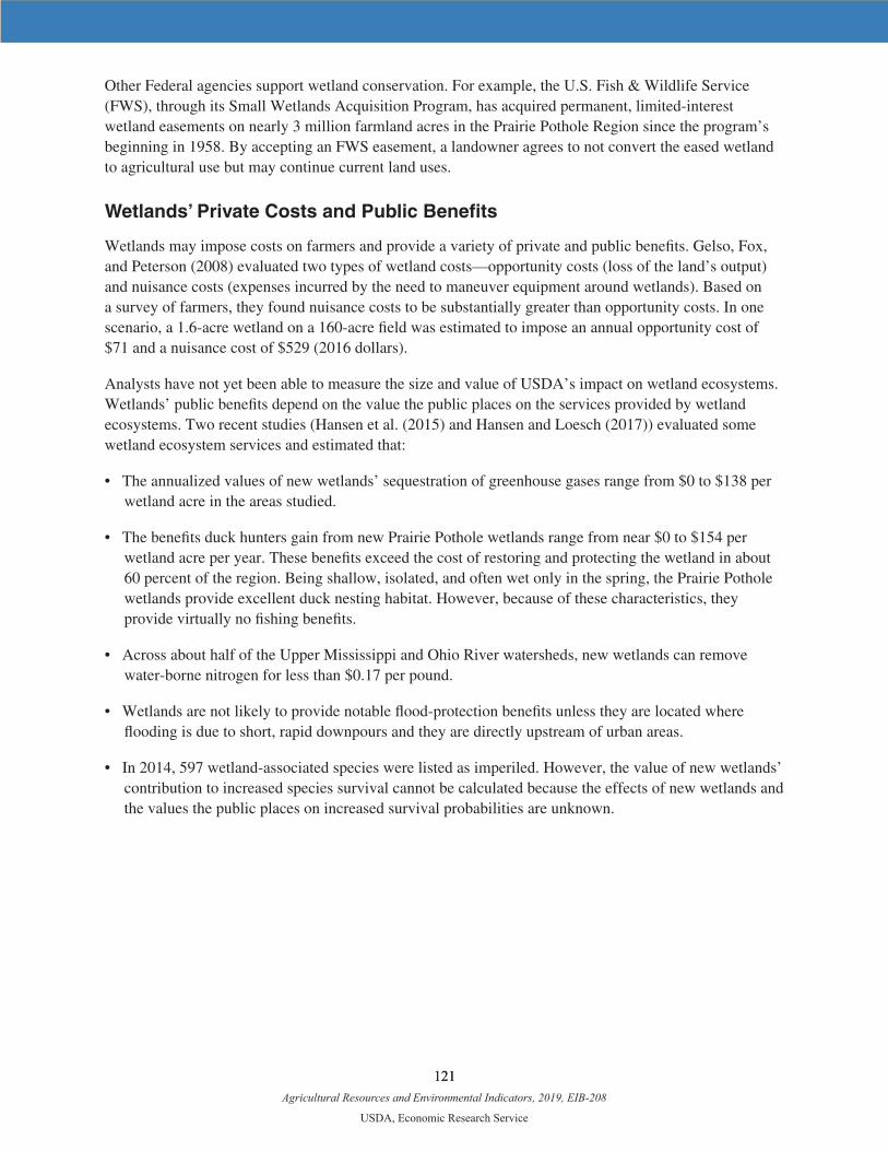
Agricultural Resources and Environmental Indicators, 2019, EIB-208
USDA, Economic Research Service
121 121
Other Federal agencies support wetland conservation. For example, the U.S. Fish & Wildlife Service (FWS), through its Small Wetlands Acquisition Program, has acquired permanent, limited-interest wetland easements on nearly 3 million farmland acres in the Prairie Pothole Region since the program’s beginning in 1958. By accepting an FWS easement, a landowner agrees to not convert the eased wetland to agricultural use but may continue current land uses.
Wetlands’ Private Costs and Public Benefits
Wetlands may impose costs on farmers and provide a variety of private and public benefits. Gelso, Fox, and Peterson (2008) evaluated two types of wetland costs—opportunity costs (loss of the land’s output) and nuisance costs (expenses incurred by the need to maneuver equipment around wetlands). Based on a survey of farmers, they found nuisance costs to be substantially greater than opportunity costs. In one scenario, a 1.6-acre wetland on a 160-acre field was estimated to impose an annual opportunity cost of $71 and a nuisance cost of $529 (2016 dollars).
Analysts have not yet been able to measure the size and value of USDA’s impact on wetland ecosystems. Wetlands’ public benefits depend on the value the public places on the services provided by wetland ecosystems. Two recent studies (Hansen et al. (2015) and Hansen and Loesch (2017)) evaluated some wetland ecosystem services and estimated that:
•Theannualizedvaluesofnewwetlands’sequestrationofgreenhousegasesrangefrom$0to$138perwetland acre in the areas studied.
•ThebenefitsduckhuntersgainfromnewPrairiePotholewetlandsrangefromnear$0to$154perwetland acre per year. These benefits exceed the cost of restoring and protecting the wetland in about 60 percent of the region. Being shallow, isolated, and often wet only in the spring, the Prairie Pothole wetlands provide excellent duck nesting habitat. However, because of these characteristics, they provide virtually no fishing benefits.
•AcrossabouthalfoftheUpperMississippiandOhioRiverwatersheds,newwetlandscanremovewater-borne nitrogen for less than $0.17 per pound.
•Wetlandsarenotlikelytoprovidenotableflood-protectionbenefitsunlesstheyarelocatedwhereflooding is due to short, rapid downpours and they are directly upstream of urban areas.
•In2014,597wetland-associatedspecieswerelistedasimperiled.However,thevalueofnewwetlands’contribution to increased species survival cannot be calculated because the effects of new wetlands and the values the public places on increased survival probabilities are unknown.
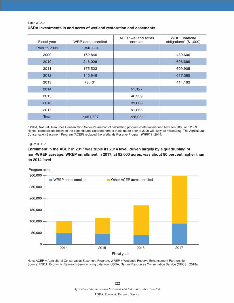
Agricultural Resources and Environmental Indicators, 2019, EIB-208
USDA, Economic Research Service
122 122
Table 3.22.2
USDA investments in and acres of wetland restoration and easements
Fiscal year WRP acres enrolledACEP wetland acres
enrolledWRP Financial
obligations* ($1,000)
Prior to 2009 1,842,284
2009 162,846 489,606
2010 246,028 696,689
2011 175,522 609,905
2012 146,646 617,385
2013 78,401 414,162
2014 51,127
2015 46,339
2016 39,603
2017 91,865
Total 2,651,727 228,934
*USDA, Natural Resources Conservation Service’s method of calculating program costs transitioned between 2008 and 2009. Hence, comparisons between the expenditures reported here to those made prior to 2009 will likely be misleading. The Agricultural Conservation Easement Program (ACEP) replaced the Wetlands Reserve Program (WRP) in 2014.
Figure 3.22.2
Enrollment in the ACEP in 2017 was triple its 2014 level, driven largely by a quadrupling of non-WREP acreage. WREP enrollment in 2017, at 92,000 acres, was about 80 percent higher than its 2014 level
Program acres
0
50,000
100,000
150,000
200,000
250,000
300,000
2014 2015 2016 2017
Fiscal year
WREP acres enrolled Other ACEP acres enrolled
Note: ACEP = Agricultural Conservation Easement Program. WREP = Wetlands Reserve Enhancement Partnership.Source: USDA, Economic Research Service using data from USDA, Natural Resources Conservation Service (NRCS), 2018a.

Agricultural Resources and Environmental Indicators, 2019, EIB-208
USDA, Economic Research Service
123 123
References
Claassen, Roger, Maria Bowman, Vince Breneman, Tara Wade, Ryan Williams, Jacob Fooks, LeRoy Han-sen, Rich Iovanna, and Chuck Loesch. 2017. Conservation Compliance: How Farmer Incentives Are Changing in the Crop Insurance Era, ERR-234, U.S. Department of Agriculture, Economic Research Service, July.
Gelso, Brett, John Fox, and Jeffery Peterson. 2008. “Farmers’ Perceived Costs of Wetlands: Effects of Wetland Size, Hydration, and Dispersion,” American Journal of Agricultural Economics 90(1):172-85, February.
Hansen, LeRoy. 2006. “Wetlands Status and Trends,” in Agricultural Resources and Environmental Indicators, 2006 Edition, K. Wiebe and N. Gollehon, eds., EIB-16, U.S. Department of Agriculture, Economic Research Service.
Hansen, LeRoy, Daniel Hellerstein, Marc Ribaudo, James Williamson, David Nulph, Charles Loesch, and William Crumpton. 2015. Targeting Investments To Cost Effectively Restore and Protect Wetland Ecosystems: Some Economic Insights, ERR183, U.S. Department of Agriculture, Economic Research Service, February.
Hansen, LeRoy, and Chuck Loesch. 2017. “Targeting Waterfowl Habitat Restoration in the Prairie Pothole Region: A Spatial Analysis of Marginal Benefits and Costs,” Journal of Soil and Water Conservation 72(4):299-307, July/August. doi: 10.2489/jswc.72.4.299
U.S. Department of Agriculture. Natural Resources Conservation Service. 2018A. “Agricultural Conser-vation Easement Program (ACEP).”
U.S. Department of Agriculture, Natural Resources Conservation Service. 2017B. “Wetlands Reserve Program (WRP).”
U.S. Department of Agriculture, Natural Resources Conservation Service. 2015. Summary Report: 2012 National Resources Inventory, Natural Resources Conservation Service, Washington, DC, and Center for Survey Statistics and Methodology, Iowa State University, Ames, IA.
U.S. Department of Agriculture, Natural Resources Conservation Service. 2013 “2007 National Resources Inventory: Wetlands.”
Agricultural Resources and Environmental Indicators, 2019, EIB-208
USDA, Economic Research Service
124 124
Chapter 3.23—Conservation Reserve Program
Daniel Hellerstein
• As of October 2018, the voluntary Conservation Reserve Program (CRP) enrolled over 22.4 million acres of environmentally sensitive cropland.
• About 35 percent of CRP acres is enrolled through continuous signups that target high-priority envi-ronmental concerns.
• Between 2012 and 2014, acceptance rates in CRP’s general signups increased from about 66 per-cent to 80 percent, but then declined to 22 percent in 2016.
Now over 30 years old, as of October 2018 the USDA’s Conservation Reserve Program (CRP) had enrolled over 22.4 million acres of environmentally sensitive cropland under 10- to 15-year contracts with qualifying landowners. With 2018 annual rental payments of around $1.8 billion, the CRP continues to be USDA’s largest conservation program (see chapter 3.21, “Conservation Spending Seeks To Improve Environmental Performance in Agriculture”).The CRP is voluntary, with eligible landowners offering to enroll land primarily under one of two meth-ods with a third option added under the 2014 Farm Act. In the first two types of enrollment, land enrolled in the CRP is retired from crop production, and the land is planted to a selected “conservation practice” such as native grasses, tree cover, or pollinator habitat. The older, and larger, method is “general signup.” General signups, which normally occur every year or few years, are several weeklong periods during which landowners can submit offers to enroll cropland in the CRP. At the end of the signup period, the program scores each offer using an Environmental Benefits Index (EBI),1 and then accepts all qualified offers that exceed a threshold score. The second enrollment type (established in 1996) is “continuous sig-nup,” which accepts offers at any time of the year, though these offers must meet more stringent eligibility criteria. There are a number of continuous signup initiatives, each with its own geographic and cover- practice requirements. The third enrollment type is CRP Grasslands enrollment, which has a continuous signup with ranking periods. Under CRP Grasslands, landowners and operators can protect grassland—in-cluding rangeland, pastureland, and certain other lands—while maintaining the areas as grazing lands.
The CRP’s size and goals have changed, from its early emphasis on limiting crop production and soil erosion to one that now considers a broad set of conservation goals including wildlife and pollinator hab-itat, as well as soil, water, and air quality. The CRP allows for grazing in limited circumstances. Driven by improvements in conservation practices and evolving legislative mandates, commodity markets, and environmental concerns, the CRP continues to adapt.
1The EBI consists of a number of different factors that account for water quality, soil erosion, wildlife habitat, and other effects of retiring a parcel of cropland. The EBI combines measures of these effects, along with the requested asking price, to produce a single score for each offer.
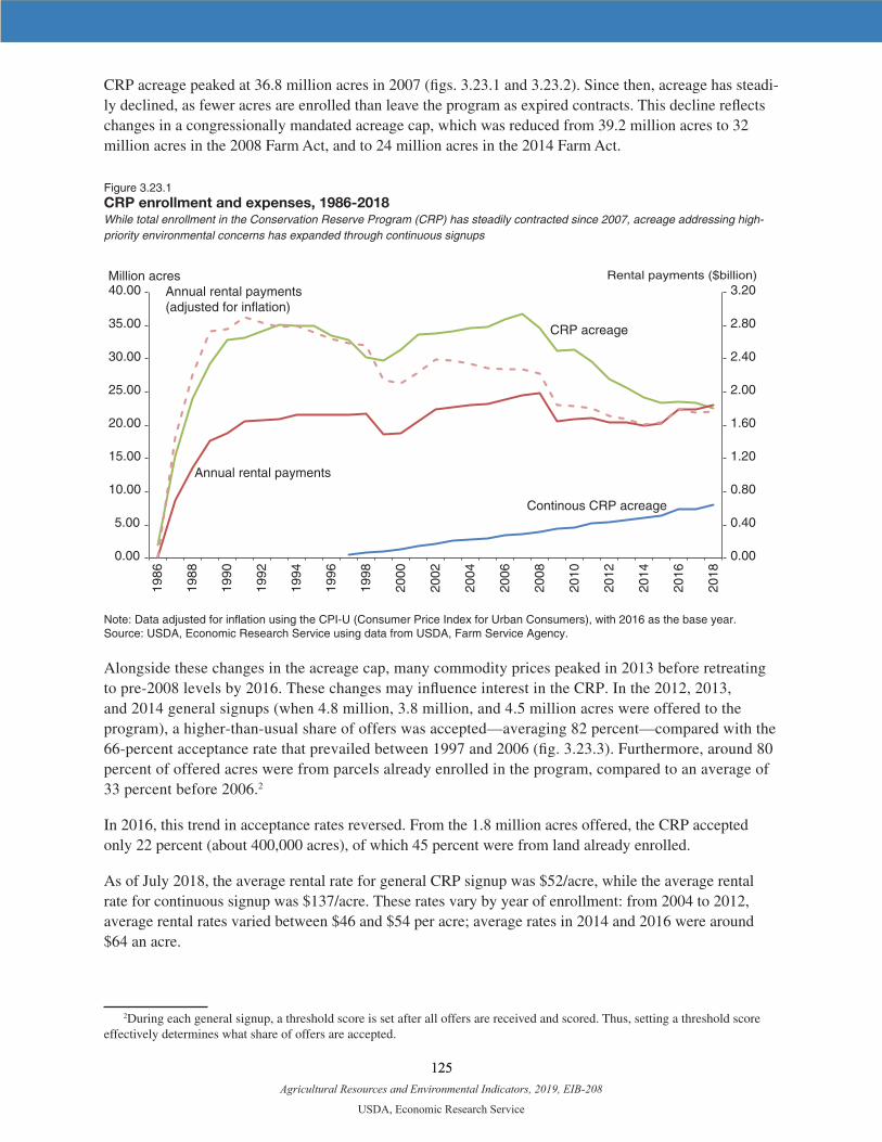
Agricultural Resources and Environmental Indicators, 2019, EIB-208
USDA, Economic Research Service
125 125
CRP acreage peaked at 36.8 million acres in 2007 (figs. 3.23.1 and 3.23.2). Since then, acreage has steadi-ly declined, as fewer acres are enrolled than leave the program as expired contracts. This decline reflects changes in a congressionally mandated acreage cap, which was reduced from 39.2 million acres to 32 million acres in the 2008 Farm Act, and to 24 million acres in the 2014 Farm Act.
Figure 3.23.1CRP enrollment and expenses, 1986-2018 While total enrollment in the Conservation Reserve Program (CRP) has steadily contracted since 2007, acreage addressing high-priority environmental concerns has expanded through continuous signups
Million acres
0.00
0.40
0.80
1.20
1.60
2.00
2.40
2.80
3.20
0.00
5.00
10.00
15.00
20.00
25.00
30.00
35.00
40.00
1986
1988
1990
1992
1994
1996
1998
2000
2002
2004
2006
2008
2010
2012
2014
2016
2018
CRP acreage
Annual rental payments
Annual rental payments(adjusted for inflation)
Continous CRP acreage
Rental payments ($billion)
Note: Data adjusted for inflation using the CPI-U (Consumer Price Index for Urban Consumers), with 2016 as the base year.Source: USDA, Economic Research Service using data from USDA, Farm Service Agency.
Alongside these changes in the acreage cap, many commodity prices peaked in 2013 before retreating to pre-2008 levels by 2016. These changes may influence interest in the CRP. In the 2012, 2013, and 2014 general signups (when 4.8 million, 3.8 million, and 4.5 million acres were offered to the program), a higher-than-usual share of offers was accepted—averaging 82 percent—compared with the 66-percent acceptance rate that prevailed between 1997 and 2006 (fig. 3.23.3). Furthermore, around 80 percent of offered acres were from parcels already enrolled in the program, compared to an average of 33 percent before 2006.2
In 2016, this trend in acceptance rates reversed. From the 1.8 million acres offered, the CRP accepted only 22 percent (about 400,000 acres), of which 45 percent were from land already enrolled.
As of July 2018, the average rental rate for general CRP signup was $52/acre, while the average rental rate for continuous signup was $137/acre. These rates vary by year of enrollment: from 2004 to 2012, average rental rates varied between $46 and $54 per acre; average rates in 2014 and 2016 were around $64 an acre.
2During each general signup, a threshold score is set after all offers are received and scored. Thus, setting a threshold score effectively determines what share of offers are accepted.

Agricultural Resources and Environmental Indicators, 2019, EIB-208
USDA, Economic Research Service
126 126
Figure 3.23.2
Conservation Reserve Program (CRP) acreage in 2018 and change in acreage, 2012-18
Change in CRP acreage: 2012-2018
2,000 or more
1 - 2,000
-24,9999 - 0
-749,999 - -25,0000
Less than -750,000
Insufficient data
<100K100K-500K500K-1,000K1,000K-1,500K>1,500K
2018 CRP acreage by State
Source: USDA, Economic Research Service analysis of contract data from USDA, Farm Service Agency, Conservation Reserve Program.
The overall decline in CRP acreage has been driven by reductions in the acreage enrolled via CRP’s general signup. However, acres enrolled through “continuous signups”—including land in one of the many State-Federal conservation partnerships under the Conservation Reserve Enhancement Program (CREP) —has steadily increased. Continuous signups target high-priority environmental concerns. In contrast to general signups, which use offer attributes (such as the asking price and the parcel’s soil erod-ibility) to rank offers, continuous signups accept all offers that meet more stringent eligibility require-ments, including location and the conservation practice to be installed. From its inception in 1999, acres enrolled through continuous signup has steadily increased, with over 2.6 million acres in 2003, 3.9 million acres in 2007, and over 5.3 million acres in 2012. As of July 2018, 35 percent of CRP land (8.1 million acres) was enrolled via continuous signup. This includes about 399,000 acres of farmable wetland, and about 989,000 acres under CREP.
CREP comprises over 45 Federal/State partnerships designed to address specific environmental objectives through targeted CRP enrollments. Acres enrolled via CREP increased from about 530,000 acres in 2003 to 980,000 acres in 2007 to 1.25 million acres in 2011, before declining to around 1.06 million acres by September 2017.

Agricultural Resources and Environmental Indicators, 2019, EIB-208
USDA, Economic Research Service
127 127
Figure 3.23.3
Conservation Reserve Program (CRP) general signup: acceptance rates and share of offers from
land already in the CRP, 1997-2016
Percent
0
10
20
30
40
50
60
70
80
90
15(1997)
16(1998)
18(1999)
20(2000)
26(2003)
29(2004)
33(2006)
39(2010)
41(2011)
43(2012)
45(2013)
49(2016)
General signup (year)
Acceptance rate
Re-enrollment rate
Note: “Acceptance rate” shows the percent of parcels offered to the CRP, during a general signup, that were accepted. A higher percent means fewer offers were rejected. “Re-enrollment rate” shows the percent of acres offered to the CRP, during a general signup, that were already in the CRP at the time of the offer.Source: U.S. Department of Agriculture, Economic Research Service using data from USDA, Farm Service Agency, Conservation Reserve Program (CRP).
Between 2012 and 2017, CRP’s general signup acreage decreased by 8.2 million acres while continuous signup acres increased by 2.1 million. Further growth in continuous signups may continue as additional targeted conservation practices and sites are proposed. For example, as of October 2017, the State Acres for Wildlife Enhancement (SAFE) initiative enrolled over 1.9 million acres (up from 700,000 acres in 2012). The Pollinator Habitat initiative (CP42) enrollment totaled over 440,000 acres (up from 18,000 in 2012), and land enrolled as Highly Erodible Land accounts for over 690,000 acres.
CRP Grasslands enrollment started in 2017, and reached 89,000 acres in September 2017. As of July 2018, 539,000 acres were enrolled under CRP Grasslands.
The environmental impacts of the CRP are varied. USDA’s Farm Service Agency (FSA)—using models developed by the Food and Agricultural Policy Research Institute (FAPRI)—estimates that in 2016, the 24 million acres of CRP land reduced sediment flow into waterways by 190 million tons, and reduced nitrogen and phosphorus by 514 and 102 million pounds (respectively). The U.S. Fish and Wildlife Service estimates that between 1992 and 2012, CRP enrollment (including 1.4 million acres of wetlands in the Prairie Pothole region) resulted in over 37 million additional ducks (USDA, FNS, 2013). CRP lands have also enhanced populations of grouse, northern bobwhite quail, ring-necked pheasants, and other grassland birds.

Agricultural Resources and Environmental Indicators, 2019, EIB-208
USDA, Economic Research Service
128 128
The future of the program is likely to depend on a variety of factors, such as:
•Thefutureofcommodityprices—willtheystabilizeatratesbelowthepeaksof2013,andhowwillinterest in the program respond to lower prices?
•TheAgricultureImprovementActof2018(2018FarmAct)raisestheacreagecapto27millionacresby 2023. In addition, the Act requires (to the maximum extent practicable) that 60 percent of acres available for CRP enrollment each year to be allocated across States based on historical State enroll-ment rates. How will these changes impact the distribution of CRP acreage?
•The2018FarmActmandatesthatSoilRentalRates(SRR)besetat85percentofestimatedcountyaverage Soil Rental Rates for general signup and 90 percent for continuous signup. If SRRs continue to be used to set bid caps, how will this effect the type of lands offered to the program?
•The2018FarmActmandates2millionacresingrasslands,andatleast8.6millionacresundercon-tinuous signup, by 2023. The Act also creates new initiatives under continuous signup, including the Clean Lakes, Estuaries and Rivers (CLEAR) initiative. How will these affect the 20-year trend of increasing share of acreage under continuous signup?
•CantheEnvironmentalBenefitsIndex(EBI)bemodifiedtouseimprovedmeasuresoftheenvironmen-tal impacts of retiring cropped fields?
References
Food and Agricultural Policy Research Institute. 2007. Estimating Water Quality, Air Quality, and Soil Carbon Benefits of the Conservation Reserve Program. University of Missouri-Columbia. FA-PRI-UMC Report #01-07.
Hellerstein, Daniel. 2017. “The US Conservation Reserve Program: the evolution of an enrollment mech-anism,” Land Use Policy 63. August.
U.S. Department of Agriculture, Farm Service Agency. 2016. Environmental Benefits of the Conservation Reserve Program.
U.S. Department of Agriculture, Farm Service Agency. 2011. Conservation Reserve Program Statistics. U.S. Department of Agriculture, Farm Service Agency. 2013. Conservation Reserve Program Annual
Summary and Enrollment Statistics, FY 2012.

Agricultural Resources and Environmental Indicators, 2019, EIB-208
USDA, Economic Research Service
129 129
Chapter 3.24—Working-Lands Conservation Programs
Steven Wallander and Jacob Fooks
• Over 95 percent of the $2.8 billion in annual financial assistance that goes to conservation practices on working lands comes through either the Environmental Quality Incentives Program (EQIP) or the Conservation Stewardship Program (CSP).
• Even though the funding levels for the programs have been comparable in recent years, CSP covers about three times as many farms and more than twice as much acreage per enrolled farm as EQIP.
• Of the 10 broad resource concerns addressed by EQIP, three concerns—water quality, plant condi-tion, and erosion—comprise more than 50 percent of total funding.
Each of the past five Farm Acts has brought significant changes to the ways in which USDA provides conservation funding for working lands (land that is in active production for crops, livestock, or forests). The major changes in these programs involve total funding levels, the distinction between conservation practices and conservation enhancements, and regional variation in the focus on different conservation resource concerns (see chapter 3.21, “Conservation Spending”). These programs provide producers with financial and technical assistance for implementing and managing a wide range of conservation practices. Other programs, such as the Conservation Reserve Program (see chapter 3.23), focus on removing farm-land from active production.
Two Programs Constitute the Majority of Working-Lands Funding
At least eight different working-lands conservation programs enrolled participants between 2014 and 2016. Many of the currently funded programs are modifications of and replacements for previous work-ing-lands programs. Some programs, such as the Wildlife Habitat Incentives Program, target very specific resource concerns. Others, such as the Regional Conservation Partnership Program and its predecessors (e.g., the former Chesapeake Bay Watershed Initiative), target specific geographic areas of concern. While all of the programs serve specific goals identified by Congress in the Farm Act, the majority of the funding and acreage receiving financial assistance through working-lands programs falls under two programs: the Environmental Quality Incentives Program (EQIP) and the Conservation Stewardship Program (CSP). While the 2018 Farm Act changes some aspects of these programs, including funding authorization levels, they remain the two largest USDA working-lands programs.
The principal objectives of EQIP, established in 1996, are to: (1) promote production and environmental quality as compatible goals, (2) optimize environmental benefits, and (3) help farmers and ranchers meet Federal, State, and local regulatory requirements. The key to this approach is the designation of standard conservation “practices,” which are specific management actions or structures implemented according to USDA, Natural Resources Conservation Service (NRCS) standards. After developing a conservation plan through either the NRCS technical assistance program or through one of NRCS’s partners, farmers seeking to participate in EQIP complete an application indicating which land on the farm will be enrolled, which resource concerns will be addressed, and what practices will be used. Contract selections are made at the State or local level.
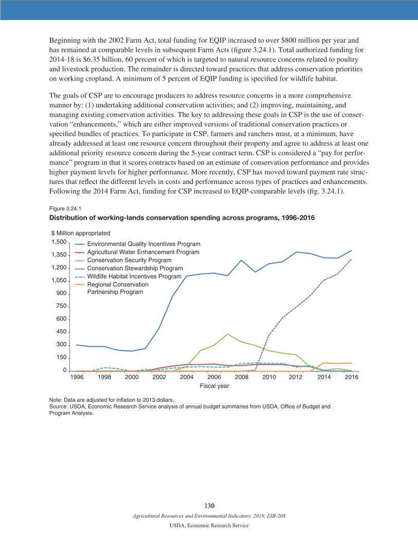
Agricultural Resources and Environmental Indicators, 2019, EIB-208
USDA, Economic Research Service
130 130
Beginning with the 2002 Farm Act, total funding for EQIP increased to over $800 million per year and has remained at comparable levels in subsequent Farm Acts (figure 3.24.1). Total authorized funding for 2014-18 is $6.35 billion, 60 percent of which is targeted to natural resource concerns related to poultry and livestock production. The remainder is directed toward practices that address conservation priorities on working cropland. A minimum of 5 percent of EQIP funding is specified for wildlife habitat.
The goals of CSP are to encourage producers to address resource concerns in a more comprehensive manner by: (1) undertaking additional conservation activities; and (2) improving, maintaining, and managing existing conservation activities. The key to addressing these goals in CSP is the use of conser-vation “enhancements,” which are either improved versions of traditional conservation practices or specified bundles of practices. To participate in CSP, farmers and ranchers must, at a minimum, have already addressed at least one resource concern throughout their property and agree to address at least one additional priority resource concern during the 5-year contract term. CSP is considered a “pay for perfor-mance” program in that it scores contracts based on an estimate of conservation performance and provides higher payment levels for higher performance. More recently, CSP has moved toward payment rate struc-tures that reflect the different levels in costs and performance across types of practices and enhancements. Following the 2014 Farm Act, funding for CSP increased to EQIP-comparable levels (fig. 3.24.1).
Figure 3.24.1
Distribution of working-lands conservation spending across programs, 1996-2016
$ Million appropriated
0
150
300
450
600
750
900
1,050
1,200
1,350
1,500
1996 1998 2000 2002 2004 2006 2008 2010 2012 2014 2016Fiscal year
Environmental Quality Incentives ProgramAgricultural Water Enhancement ProgramConservation Security ProgramConservation Stewardship ProgramWildlife Habitat Incentives ProgramRegional Conservation Partnership Program
Note: Data are adjusted for inflation to 2013 dollars.Source: USDA, Economic Research Service analysis of annual budget summaries from USDA, Office of Budget and Program Analysis.
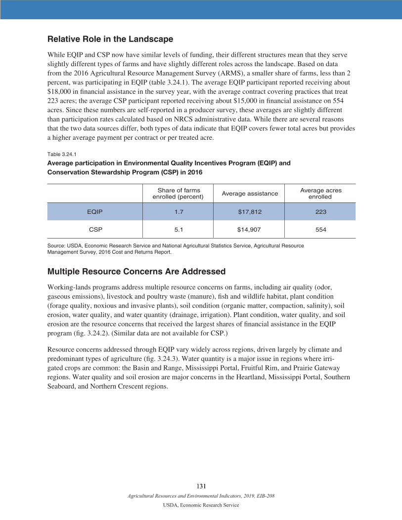
Agricultural Resources and Environmental Indicators, 2019, EIB-208
USDA, Economic Research Service
131 131
Relative Role in the Landscape
While EQIP and CSP now have similar levels of funding, their different structures mean that they serve slightly different types of farms and have slightly different roles across the landscape. Based on data from the 2016 Agricultural Resource Management Survey (ARMS), a smaller share of farms, less than 2 percent, was participating in EQIP (table 3.24.1). The average EQIP participant reported receiving about $18,000 in financial assistance in the survey year, with the average contract covering practices that treat 223 acres; the average CSP participant reported receiving about $15,000 in financial assistance on 554 acres. Since these numbers are self-reported in a producer survey, these averages are slightly different than participation rates calculated based on NRCS administrative data. While there are several reasons that the two data sources differ, both types of data indicate that EQIP covers fewer total acres but provides a higher average payment per contract or per treated acre.
Table 3.24.1
Average participation in Environmental Quality Incentives Program (EQIP) and Conservation Stewardship Program (CSP) in 2016
Share of farms enrolled (percent) Average assistance Average acres
enrolled
EQIP 1.7 $17,812 223
CSP 5.1 $14,907 554
Source: USDA, Economic Research Service and National Agricultural Statistics Service, Agricultural Resource Management Survey, 2016 Cost and Returns Report.
Multiple Resource Concerns Are Addressed
Working-lands programs address multiple resource concerns on farms, including air quality (odor, gaseous emissions), livestock and poultry waste (manure), fish and wildlife habitat, plant condition (forage quality, noxious and invasive plants), soil condition (organic matter, compaction, salinity), soil erosion, water quality, and water quantity (drainage, irrigation). Plant condition, water quality, and soil erosion are the resource concerns that received the largest shares of financial assistance in the EQIP program (fig. 3.24.2). (Similar data are not available for CSP.)
Resource concerns addressed through EQIP vary widely across regions, driven largely by climate and predominant types of agriculture (fig. 3.24.3). Water quantity is a major issue in regions where irri-gated crops are common: the Basin and Range, Mississippi Portal, Fruitful Rim, and Prairie Gateway regions. Water quality and soil erosion are major concerns in the Heartland, Mississippi Portal, Southern Seaboard, and Northern Crescent regions.

Agricultural Resources and Environmental Indicators, 2019, EIB-208
USDA, Economic Research Service
132 132
Figure 3.24.2
Distribution of Environmental Quality Incentives Program contract obligations by resource concern, 2011-13
Air quality, 3%
Domestic animals, 10%
Energy, 1%
Fish and wildlife, 11%
Plant condition22%
Soil condition10%
Soil erosion19%
Water quality19%
Water quantity, 8%
Note: Contracts that address multiple resource concerns have total obligations divided equally between those concerns for purposes of calculating the shares of funding for each concern.Source: USDA, Economic Research Service analysis of data from USDA, Natural Resources Conservation Service, ProTracts database.
Figure 3.24.3
Distribution of Environmental Quality Incentives Program contract obligations by resource concern and region, 2011-13
0
10
20
30
40
50
60
70
80
90
100
Basin andRange
EasternUplands
Fruitful Rim Heartland MississippiPortal
NorthernCrescent
NorthernGreat Plains
PrairieGateway
SouthernSeaboard
Water quantityWater qualitySoil erosionSoil conditionPlant conditionFish and wildlifeEnergyDomestic animalsAir quality
Percent
Note: Contracts that address multiple resource concerns have total obligations divided equally between those concerns for purposes of calculating the shares of funding for each concern. Contracts are assigned to regions based on administrative county codes. Source: USDA, Economic Research Service analysis of data from USDA, Natural Resources Conservation Service, ProTracts database.

Agricultural Resources and Environmental Indicators, 2019, EIB-208
USDA, Economic Research Service
133 133
References
Bowman, Maria, Steven Wallander, and Lori Lynch. 2016. “An Economic Perspective on Soil Health,” Amber Waves, U.S. Department of Agriculture, Economic Research Service, September 6.
Claassen, Roger, Maria Bowman, Jonathan McFadden, David Smith, and Steven Wallander, 2018. Tillage Intensity and Conservation Cropping in the United States. EIB-197, U.S. Department of Agriculture, Economic Research Service, September.
Wallander, Steven, Marcel Aillery, Daniel Hellerstein, and Michael Hand. 2013. The Role of Conservation Programs in Drought Risk Adaptation, ERR-148, U.S. Department of Agriculture, Economic Research Service, April.

Appendix: Data Sources
Agricultural Resources and Environmental Indicators, 2019, EIB-208
USDA, Economic Research Service
134
Chapter 1.1: Farm Numbers and Size
To follow long run trends in farm numbers, the chapter uses farm counts from the 1850 to 2012 Censuses of Agriculture. The 2012 census is the latest available; the 2017 census will be released during the spring of 2019. The chapter uses the 2017 Agricultural Resource Management Survey (ARMS) to examine farms by size of farm, measuring farm size by gross revenue. USDA’s National Agricultural Statistics Service (NASS) is currently conducting the 2018 ARMS, for release in December 2019.
Chapter 1.2: Major Land Uses in the United States
This chapter relies nearly exclusively on data from ERS’s Major Land Uses (MLU) data product, which provide the most comprehensive national accounting of land use in the United States. The data were most recently updated in August 2017 to provide information for 2012. There is one component of the MLU data that is updated annually for the Nation as a whole (cropland used for crops). The cropland used for crops data are presented in figure 1.2.3, along with other cropland uses that are not included in the annual update (cropland pasture and cropland idled).
Chapter 1.3: Farmland Values
The land values data come from NASS’s June Area Survey. This data is updated annually and reported in NASS’s Land Values summary report and Quick Stats database. The most recent update was released in August 2018.
Chapter 1.4: Farmland Ownership and Tenure
This chapter uses data from the 2014 Tenure, Ownership, and Transition of Agricultural Land (TOTAL) Survey. The TOTAL Survey constitutes the most recent effort (since 1999’s Agricultural Economics and Land Ownership Survey) to provide comprehensive information on farmland ownership arrangements, landlord-tenant agreements, owner characteristics, and farmland acquisition and transfer plans.
Chapter 1.5: Agricultural Productivity and Sources of Growth in the U.S. Farm Sector
The productivity chapter draws data mainly from the ERS “Agricultural Productivity in the U.S.” dataset, which was released October 2017. The U.S. productivity dataset provides estimates of total factor productivity (TFP) and prices and quantities of 10 outputs and 12 inputs in the U.S. farm sector for 1948-2015. The next updates are expected to be released in late 2019.
Chapter 1.6: Agricultural Research and Development
Data sources are Current Research Information System (USDA, National Institute of Food and Agriculture); Survey of Federal Funds for Research and Development (National Science Foundation, NSF); ERS compilations of data from multiple private sector sources following the methodology used in ERR-130; Business R&D and Innovation Survey (BRDIS—NSF). Public sector data are presented through 2015, the last year Federal Funds Survey data are available. Private sector data are presented through 2014, the last year for which data are available from BRDIS.
Chapter 2.7: Biotechnology, Seed Use, and Pest Control for Major U.S. Crops
Data from ERS’s Agricultural Economic Report No. 810, the NASS June Area Survey (2000-2018), the U.S. Geological Survey’s Agricultural Pesticide Use database (2000-2014), and a proprietary data source (1998-2017) were used to create the figures and tables in this chapter.
Chapter 2.8: Pest Management
Data are from several sources, including the U.S. Environmental Protection Agency, Pesticides Industry Sales and Usage report (2017); U.S. Geological Survey data on estimated annual agricultural pesticide use by crop group for conterminous States, and recent NASS QuickStats data (up to 2016). For some figures, proprietary data were used. Differences in the time periods discussed in chapters 2.7 and 2.8 stem from differences in the datasets analyzed.
Chapter 2.9: Nutrient Management
Data include USDA, Economic Research Service Fertilizer Use and Price, based on “Commercial Fertilizers 2014,” published in July 2017; the latest commodity-specific Phase II surveys—corn, 2016; cotton, 2015; soybeans, 2012; and winter wheat, 2009.
Chapter 2.10: U.S. Irrigated Agriculture: Farm Structure, Technology, and Conservation
Data are from the 2012 Census of Agriculture, the 2013 Farm & Ranch Irrigation Survey (FRIS), and (to a lesser degree) the 2010 USGS Water Estimates report. No new irrigation/water data will be available until late 2019. Numbers will not be available from the 2017 Census of Agriculture until the spring of 2019. The 2018 FRIS went out into the field in January 2019, with data expected in late 2019. USGS is still working on its 2015 Water Estimates report (no expected date for release).
Appendix: Data Sources

Agricultural Resources and Environmental Indicators, 2019, EIB-208
USDA, Economic Research Service
135 135
Chapter 2.11: Precision Agriculture
Data are from crop-specific ARMS surveys, conducted from 1996 to 2016. ARMS surveys are done annually, with 2017 information scheduled for release in the latter part of 2019. ARMS collects very detailed information on production practices and is conducted annually for one or two crops.
Chapter 2.12: Crop Production Management: Tillage Practices
No-till and strip-till adoption rates are estimated using the farm-level portion of the 2010 and 2011 ARMS and field-level ARMS for soybeans in 2012, cotton in 2015, corn in 2016, and wheat in 2017. The data are presented by crop and region. In the farm-level surveys, farmers were asked to report the acreage of corn, soybeans, wheat, and cotton where no-till/strip-till was used in the survey year. The 2010-11 farm-level surveys are the only farm wide ARMS tillage data available. In the field-level surveys, farmers’ tillage use reflects the absence of tillage operations in the survey year; prior-year data are based on producer recall. Field-level ARMS are crop-year specific and conducted annually.
Chapter 2.13: U.S. Organic Farming Systems
Data on organic production are from USDA-ARMS surveys, including the 2006 ARMS soybean survey, 2007 ARMS apple survey, 2009 ARMS wheat survey, and 2010 ARMS corn survey; these ARMS commodity surveys contained targeted over-samples of organic producers to ensure statistically reliable data for production stratified by farming system. Data from the most recent (2012) Census of Agriculture and the 2014 National Organic Producer Survey follow-on census are also used, as is data from 2006-2016 from USDA’s National Organic Program Integrity database. The most recent data from USDA’s Natural Resources Conservation Service on conservation program (EQIP) funding for organic and transition practices—from 2009 (when funding for these practices was initiated) through 2016—are also used. Data on U.S. organic product market share are from the market research company IRI for the 2009-14 period, and data on U.S. organic retail sales are from the Nutrition Business Journal and Organic Trade Association through 2017.
Chapter 2.14: Manure Management
Figure 2.14.1 uses the 2012 Census; the 2017 Census will be released in the spring of 2019. Tables 2.14.1 and 2.14.2 use the 2009 hog, 2010 dairy, and the 2011 broiler surveys. The broiler survey is the latest available, with no date set for a future survey. More recent hog and dairy surveys (2015 hogs, 2016 dairy) do not ask detailed questions about manure handling (e.g., how the manure was applied, whether and how it was removed, whether the operation has a nutrient management plan, whether the operation adjusted manure nutrient content via feed, or whether the farm received EQIP payment for manure management), and so were not used.
Chapter 2.15: Antibiotic Use in U.S. Livestock Production
Data on broilers raised without antibiotics except for disease treatment are from the 2006 and 2011 ARMS broiler surveys. The 2011 broiler survey is the latest available, with no date set for a future survey. The 2017 statistic on broilers produced under product lines termed “raised without antibiotics” is from USDA AMS Agricultural Analytics. Data from the 2004, 2009, and 2015 ARMS hog surveys are used to estimate the percentage of hogs that were administered antibiotics for growth promotion; the 2015 hog survey is the latest available. Statistics quoted from APHIS’s National Animal Health Monitoring System (NAHMS) use the most recent surveys available.
Chapter 3.16 Farm-Level Adaptation to Drought Risk
Data on crop insurance and drought comes from USDA, Risk Management Agency’s publicly available “Summary of Business – Cause of Loss” files and is adjusted using ERS farm-income data. Data for the drought risk measure come from publicly available National Oceanic and Atmospheric Administration (NOAA) Palmer Drought Index historical data from 1900 to 2016. The data on irrigated cropland are from the Census of Agriculture publicly available county-level data and are up to date (1998-2013). The tile drainage map is from a special requested dataset from NASS from the 2012 Census of Agriculture.
Chapter 3.17: Water Quality: Pollutants From Agriculture
Data are from the 2012 Census of Agriculture and the USGS Pesticide National Synthesis Project (1992-2014). We also use the EPA 2017 Water Quality Assessment. The most recent USGS Pesticide National Synthesis Project data are available for 2015. We choose not to use the 2015 data because there was a major shift in methodology in 2015. Starting in that year, no data on seed treatments were reported.

Agricultural Resources and Environmental Indicators, 2019, EIB-208
USDA, Economic Research Service
136 136
Chapter 3.18: Renewable Energy
Data are from the 2012 Census of Agriculture for estimates of the share of farms with on farm renewable production systems. These are the most recent data available, as ARMS does not ask about renewable production systems. Additional data are from the 2014 ARMS, since that survey asked about royalty income from wind leases. In later ARMS surveys, it is not possible to disentangle wind lease income from oil/gas royalty income. Data on biofuel production are from 2018 updates to ERS’ U.S. Bioenergy data and EIA’s Monthly Energy Review.
Chapter 3.19: Soil Health
Data are from the 2012 Census of Agriculture, the 2015 Agricultural Resource Management Survey, administrative data on programs administered by the USDA Natural Resources Conservation Service, and the 2012 NRCS National Resources Inventory (NRI). Administrative data–from 2015 and 2016–on EQIP and CSP program acreages and expenditures are the most recent data provided to ERS by NRCS. Census of Agriculture data are some of the most geographically comprehensive data on adoption of soil health and conservation practices in the United States. Updated NRI data, for 2017, are likely to be released in 2019.
Chapter 3.20: Pollinators: Honey Bee Status and Trends
The pollinator chapter uses data from the annual USDA/NASS Honey Report; using the 2018 version containing data for 2017 available at time of publication. USDA/NRCS National Resources Inventory data, from 1982 to 2012 (the most recent year available) are also used.
Chapter 3.21: Conservation Spending Seeks To Improve Environmental Performance in Agriculture
Data on conservation program spending run through fiscal year 2017. These data are updated annually based on the USDA budget summary released, along with the President’s budget. The figure, Conservation Program Spending, Fiscal Years 1996-2017, is updated on the ERS conservation programs topic page annually.
Chapter 3.22: Wetlands: Status and Trends
This chapter uses National Resources Inventory summary data (USDA/NRCS (2015)). Wetlands Reserve Program contract acreage and financial obligations were taken from a 2017 USDA/NRCS report, as were details on the Agricultural Conservation Easement Program (ACEP) wetland acreage and obligations. Details on CRP wetlands are derived from 2018 USDA/FSA reports on the CRP. These data sources are updated periodically; the studies used here were the latest available when this chapter was drafted.
Chapter 3.23: Conservation Reserve Program
Data are from reports regularly produced by the USDA Farm Service Agency (FSA). In addition, historical trend data are based on yearly contract data from FSA, the most recent being from the end of fiscal year 2017 (September 30, 2017). Also, FSA offer data from CRP’s general signups (1996-2016) are used.
Chapter 3.24: Working-Lands Conservation Programs
Data on EQIP participation are from the 2016 ARMS Phase 3 survey. The data on program expenditures are publicly available and are through 2016. The data on resource concerns are from an ERS analysis of the 2011 to 2013 NRCS ProTracts database.