Adaptive multiresolution approach for two-dimensional PDEs

Comput. Methods Appl. Mech. Engrg. 193 (2004) 405–425

www.elsevier.com/locate/cma

Adaptive multiresolution approach for two-dimensional PDEs

J.C. Santos a, P. Cruz a, M.A. Alves b,*, P.J. Oliveira c,F.D. Magalh~aaes a, A. Mendes a

a LEPAE–Departamento de Engenharia Qu�ıımica, Faculdade de Engenharia da Universidade do Porto,

Rua Dr. Roberto Frias, 4200-465 Porto, Portugalb Departamento de Engenharia Qu�ıımica, CEFT, Faculdade de Engenharia da Universidade do Porto,

Rua Dr. Roberto Frias, 4200-465 Porto, Portugalc Departamento de Engenharia Electromecaanica, Universidade da Beira Interior,

Rua Marquees d’�AAvila e Bolama, 6201-001 Covilh~aa, Portugal

Received 18 March 2003; received in revised form 6 October 2003; accepted 13 October 2003

Abstract

A multiresolution adaptive approach for the solution of two-dimensional partial differential equations (PDEs) is

presented. This methodology is a multidimensional extension of that presented in a previous work [Comput. Methods

Appl. Mech. Engrg. 191 (2002) 3909]. The method proposed is unconditionally stable, by incorporating convection

differencing schemes with the TVD property, and the grid is dynamically adapted so that higher spatial resolution is

automatically allocated to domain regions where strong gradients are observed. The two desired properties of any PDE

solver, stability and accuracy, are therefore retained. Numerical results for four test problems are presented which serve

to demonstrate the robustness and cost effectiveness of the method.

� 2003 Elsevier B.V. All rights reserved.

Keywords: Adaptive grid; CUBISTA high-resolution scheme; Multiresolution; Hyperbolic equations; Wavelet

1. Introduction

Solution of partial differential equations (PDEs) is a key ingredient in many problems of physics and

engineering and so it is a subject of active research in numerical analysis. In a previous work by our group

[1], we have introduced a multiresolution strategy coupled with high-order bounded difference schemes,

which was shown to be very effective in solving one-dimensional problems involving hyperbolic PDEs with

or without sharp fronts. This forms the basis for the present contribution, in which a general class of 2D

non-linear advection–diffusion–reaction equations of the form

* Corresponding author. Fax: +351-22-508-1449.

E-mail address: [email protected] (M.A. Alves).

0045-7825/$ - see front matter � 2003 Elsevier B.V. All rights reserved.

doi:10.1016/j.cma.2003.10.005

mail to: [email protected]

406 J.C. Santos et al. / Comput. Methods Appl. Mech. Engrg. 193 (2004) 405–425

ouot

þ oF ðx; y; t; uÞox

þ oGðx; y; t; uÞoy

¼ to

oxQðuÞ ou

ox

� ��þ o

oyRðuÞ ou

oy

� ��þ Sðx; y; t; uÞ ð1Þ

with initial values uðt ¼ 0; x; yÞ ¼ u0ðx; yÞ is considered. The main focus will be on the hyperbolic equations

that occur when Eq. (1) is dominated by advection (t ! 0). These are the typical equations governing

transport phenomena at high Reynolds (or Peclet) numbers, which are known to be difficult to solve

numerically in many cases.

The methodology we propose requires the use of high-resolution schemes combined with an adaptive

mesh technique inspired by wavelet theory. In this approach, higher-order accuracy is combined with a

multiresolution mesh refinement technique in order to achieve a nearly constant discretization error

throughout the computational domain, thus reducing the memory and CPU requirements of the solver,while keeping the same level of accuracy with respect to the equivalent uniform mesh approach. A new

high-resolution scheme is also explained.

Since an introduction to the proposed multiresolution methodology was already given in our previous

paper [1] we may condense here the background points. The basic idea of multiresolution analysis was put

forward by Mallat [2] in the context of orthonormal wavelets. Later, Harten [3] has set a general framework

for multiresolution representation, with view to reducing the number of flux computations when expensive

methods, such as ENO schemes, are employed (see also [4]). There are other approaches similar to Harten�smethodology such as the ones proposed by Cohen et al. [5]. Karni et al. [6] proposes a smoothness indicatorfor the solution of hyperbolic conservation laws. This indicator is a practical tool to identify where grid

adaptation is needed.

Harten�s methodology produces moderate CPU reductions but it is limited because, for each time step,

the solution is still represented on the finest grid. A better strategy is to couple dynamical mesh adaptation

with multiresolution and deal specifically with the restricted solution domain where sharp gradients are

present. Then it is advantageous to store only the significant information and perform the time integration

in this reduced set of grid points. There is, however, the need to dynamically adapt the mesh as the solution

evolves but, as will be demonstrated, this overhead is not significant and globally there are significantmemory and CPU time savings as compared to the corresponding fixed grid approach.

This paper is organized as follows: first, high-resolution schemes are broadly described and a new

scheme, called CUBISTA [7], is introduced. Then, the multiresolution representation of data in 2D is

explained together with interpolation procedures, followed by a description of the grid adaptation

strategy and the way to determine spatial derivatives in the adapted grid. The overall methodology is

applied to the solution of four test cases, which include hyperbolic PDEs with very strong gradients and

the classical shock-tube problem of gas dynamics. The paper ends with a summary of the main con-

clusions.

2. The high-resolution scheme

A key point in the discretization of Eq. (1) is the treatment of the convection term, in order to prevent

the appearance and subsequent intensification of unnatural oscillations. For this purpose, high-resolution

schemes are used, as explained by Leonard in two excellent review articles on this matter [8,9]. Such

schemes require normalizing the relevant advected variables and prescribing an interpolation procedure in anormalized variable diagram (the NVD). Since we have described this matter in [1], we shall give here the

minimum details to make this section easy to follow. For each direction x and y we must identify upstream

(U) and downstream (D) nodes relative to the central grid point (P), as represented in Fig. 1, so that the

normalized cell-face value of the convected flux, / (� F or G depending on the direction being evaluated) is

given by [10]

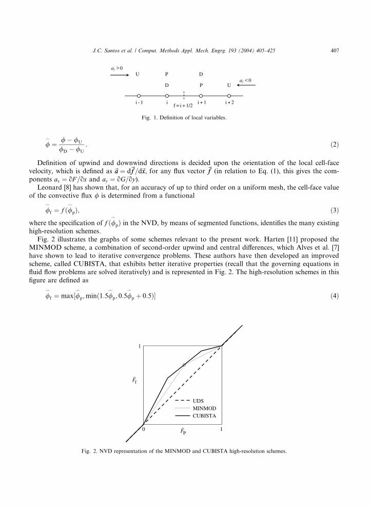
f = i + 1/2

U P D

D P U

i - 1 i i + 1 i + 2

0fa >

0fa <

Fig. 1. Definition of local variables.

J.C. Santos et al. / Comput. Methods Appl. Mech. Engrg. 193 (2004) 405–425 407

/_

¼ /� /U

/D � /U

: ð2Þ

Definition of upwind and downwind directions is decided upon the orientation of the local cell-face

velocity, which is defined as ~aa ¼ d~ff =d~xx, for any flux vector ~ff (in relation to Eq. (1), this gives the com-

ponents ax ¼ oF =ox and ay ¼ oG=oy).Leonard [8] has shown that, for an accuracy of up to third order on a uniform mesh, the cell-face value

of the convective flux / is determined from a functional

/_

f ¼ f ð/_

pÞ; ð3Þ

where the specification of f ð/_

pÞ in the NVD, by means of segmented functions, identifies the many existing

high-resolution schemes.

Fig. 2 illustrates the graphs of some schemes relevant to the present work. Harten [11] proposed the

MINMOD scheme, a combination of second-order upwind and central differences, which Alves et al. [7]

have shown to lead to iterative convergence problems. These authors have then developed an improved

scheme, called CUBISTA, that exhibits better iterative properties (recall that the governing equations in

fluid flow problems are solved iteratively) and is represented in Fig. 2. The high-resolution schemes in this

figure are defined as

/_

f ¼ max½/_

p;minð1:5/_

p; 0:5/_

p þ 0:5Þ� ð4Þ

PF

fF

1

1

UDS MINMODCUBISTA

0 )

)

Fig. 2. NVD representation of the MINMOD and CUBISTA high-resolution schemes.


for MINMOD, and

/_

f ¼ max½/_

p;minð1:75/_

p; 0:75/_

p þ 0:375; 0:25/_

p þ 0:75Þ� ð5Þ

for CUBISTA. We note that these equations are written for uniform meshes and may be easily re-inter-

preted in terms of non-uniform meshes (see [1,7]) following the Normalised Variable and Space Formu-

lation (NVSF) of [10].

Once the high-resolution convection scheme is specified, the task of computing the cell-face value of the

dependent variable is straightforward, and is described in detail in [1].

3. Multiresolution representation of data

As explained in the Introduction, the idea of this work is to extend to two-dimensional grids the ap-

proach followed in Alves et al. [1].

Consider a set of dyadic grids of the form

V j ¼ fðxjk; yjlÞ 2 R2 : xjk ¼ 2�jk; yjl ¼ 2�jlg; j; k; l 2 Z; ð6Þ

where j identifies the resolution level, k the spatial location for the x-direction and l the spatial location for

the y-direction, as illustrated in Fig. 3. Both the x and y dimensions of the computational domain have been

normalized, so that the corresponding co-ordinates vary between 0 and 1.

Assume that the solution is known on grid V j and that we want to extend it to the next finer grid V jþ1,

which has four times more points than the previous grid (note that in 1D, the factor is only 2). For the even-numbered grid points, in both directions of grid V jþ1, we already know their values, which are given by

ujþ12k;2l ¼ ujk;l: ð7Þ

The values in the odd-numbered grid points in V jþ1 for x-direction, uðxjþ12kþ1; y

jlÞ, y-direction, uðx

jk; y

jþ12lþ1Þ or

both u xjþ12kþ1; y

jþ12lþ1

� �are computed by interpolating the known even-numbered grid points in the same

direction. Then, for a certain number of time steps, the solution on a given mesh ðxk; ylÞ is advanced in timewith the solver specified in Section 4, until a new mesh adaptation step is reached (see [1]). Mesh points will

Fig. 3. Example of points in a dyadic grid: (d) V 2 and (�) V 3.


be added in zones where the solution changes abruptly, according to interpolative error coefficients definedby the difference between the existing solution value uk;l and the value obtained by interpolation from

neighbour nodal points, Iðuk;lÞ (it is noted that interpolation is only required in odd-numbered points). In

two dimensions 4 types of interpolation are possible, in contrast with the single one for the 1D case of the

previous work [1]. The interpolative error coefficients for the jth resolution level are obtained by the fol-

lowing steps:

1. For odd-numbered grid points in x-direction and even-numbered in y-direction:

dj1;k;l ¼ u xjþ1

2kþ1; yjl

� �� Ijx u xjþ12kþ1; y

jl

� �� uref ; k; l ¼ 0 to 2j: ð8Þ

Here Ijx is the interpolating operator, based on function values along the x-direction for constant y-coordinate: uðxjk�1; y

jlÞ, uðx

jk; y

jlÞ, uðx

jkþ1; y

jlÞ and uðxjkþ2; y

jlÞ (see Fig. 4(a)). We suggest the use of the known

maximum value of the dependent variable for the reference value of the dependent variable, uref .

Fig. 4. Illustration of the grid points used by the interpolating operators: (a) Ijx ½uðxjþ12kþ1; y

jlÞ�, (b) I jy ½uðx

jk ; y

jþ12lþ1Þ�, (c) Ijx ½uðx

jþ12kþ1; y

jþ12lþ1Þ� and

(d) Ijy ½uðxjþ12kþ1; y

jþ12lþ1Þ�.


2. For odd-numbered grid points in y-direction and even-numbered in x-direction:

dj2;k;l ¼ u xjk; y

jþ12lþ1

� �� Ijy u xjk; yjþ12lþ1

� �� .uref ; k; l ¼ 0 to 2j; ð9Þ

where Ijy is the interpolating operator based on the function values along the y-direction, for constant x-coordinate: uðxjk; y

jl�1Þ, uðx

jk; y

jlÞ, uðx

jk; y

jlþ1Þ and uðxjk; y

jlþ2Þ (see Fig. 4(b)).

Finally, for odd-numbered grid points in both directions:

3: dj3;k;l ¼ u xjþ1

2kþ1; yjþ12lþ1

� �� I jx uðxjþ12kþ1; y

jþ12lþ1Þ

� ��uref ; k; l ¼ 0 to 2j; ð10Þ

4: dj4;k;l ¼ u xjþ1

2kþ1; yjþ12lþ1

� �� I jy uðxjþ12kþ1; y

jþ12lþ1Þ

� ��.uref ; k; l ¼ 0 to 2j; ð11Þ

where dj3;k;l is the interpolative error coefficient based in the Ijx operator (see Fig. 4(c)) and dj

4;k;l theinterpolative error coefficient based in the Ijy operator (see Fig. 4(d)). The interpolation designated by

functions Ix and Iy above is not a simple arithmetic averaging but rather is obtained with the practice

explained in the next paragraphs.

A common practice in wavelet-based methods is to utilize symmetric interpolating polynomials

[12,13], but we found that it is important to retain consistency with the discretization used for the con-

vection term. Therefore we propose using the high-resolution schemes of the previous section for inter-

polation.The procedure followed consists on the following steps, where the calculation of the interpolated values

is illustrated for the case of odd numbered grid points in x-direction and even-numbered in y-direction.

(i) Calculate the face velocity, af , to identify the local convective flux direction:

af ¼ ðajk;l þ ajkþ1;lÞ=2: ð12Þ

(ii) Calculate the normalised face value of the advected variable, u_f , using the CUBISTA high-resolution

scheme:

u_f ¼

maxujk;l�ujk�1;l

ujkþ1;l�ujk�1;l

;min7

4

ujk;l�ujk�1;l


;3

4

ujk;l�ujk�1;l


þ3

8;3

4þ1

4

ujk;l�ujk�1;l


!" #if afP0;

maxujkþ1;l�ujkþ2;l

ujk;l�ujkþ2;l

;min7

4

ujkþ1;l�ujkþ2;l

ujk;l�ujkþ2;l

;3

4

ujkþ1;l�ujkþ2;l

ujk;l�ujkþ2;l

þ3

8;3

4þ1

4

ujkþ1;l�ujkþ2;l

ujk;l�ujkþ2;l

!" #if af < 0:

8>>>>><>>>>>:

ð13Þ(iii) Calculate the interpolated value:

uf ¼ Ijx ½uðxjþ12kþ1; y

jlÞ� ¼

ujk�1;l þ u_

fðujkþ1;l � ujk�1;lÞ if af P 0;

ujkþ2;l þ u_

fðujk;l � ujkþ2;lÞ if af < 0:

8<: ð14Þ

The interpolative error coefficients in a given direction are a measure of the local ‘‘irregular’’ behaviour

of the analysed function, in that direction. If the absolute value of dj1;k;l or d

j2;k;l, is below a given (small)

threshold e, then the corresponding grid point ðxjþ12kþ1; y

jlÞ or ðxjk; y

jþ12lþ1Þ is superfluous for accurate repre-

sentation of the original function, and so those values can be rejected without loss of significant information

since the function can be reconstructed from the preserved information on the next coarser grid, V j.However, in order to reject the point ðxjþ1

2kþ1; yjþ12lþ1Þ we note that both coefficients dj

3;k;l and dj4;k;l must be below

the given threshold e.


A function that varies abruptly only in a narrow area of the domain will have most of the dji;k;l coefficients

close to zero and so the information can be compressed with great efficiency, and without loss of accuracy.

2D multiresolution approaches have been extensively studied in other contexts such as image com-

pression, and the interested reader is referred to the work of Zhou [14].

Finally, it should be noted that the multiresolution approach must select the relevant grid points in a 2D

tree structure. For example, if the point ðxjþ12kþ1; y

jþ12lþ1Þ is retained in the adaptation algorithm, then the grid

points in the x-direction ðxji¼k�mþ1;kþm; yjþ12lþ1Þ and y-direction ðxjþ1

2kþ1; yji¼l�mþ1;lþmÞ with m ¼ �1 to 2 must be

preserved, in order to be possible to reconstruct the function value in the next adaptation step, and evaluate

dj3;k;l or d

j4;k;l.

In our algorithm, the user must specify the maximum resolution level, Jmax, so that grid coalescence inproblematic regions is avoided. The user also supplies the minimum level of resolution, Jmin, and all the grid

points pertaining to this level of resolution are always conserved throughout the computations.

4. Grid adaptation and temporal integration

The PDEs are advanced in time with LSODA [15], a public domain solver for first-order ordinary

differential equation (ODE); the same solver was employed in our previous work [1]. This is a quite versatileroutine which uses either Adams�s method with an accuracy of up to 12th order, or Gear�s method for the

case of stiff problems, allowing for variable time steps and guaranteeing highly accurate solutions for the

time evolution. The inaccuracies in the computed solution are therefore mainly controlled by the spatial

discretization, and so are related to the high-resolution schemes of Section 2.

During the solution of a PDE the grid should be continuously adapted, so that it can automatically

adjust to reflect modifications in time of the solution.

4.1. Strategy

The grid adaptation strategy that is proposed for the solution of PDEs is now described. Given discrete

function values uðx; yÞ at time t ¼ t1, proceed as follows:

1. Starting in j ¼ Jmin.

2. Compute the interpolative error coefficient for odd-numbered grid points in the x-direction and even in

y-direction, dj1;k;l (see Eq. (8) and Fig. 5), for k ¼ 0 to 2j � 1 and l ¼ 0 to 2j.

3. Compute the interpolative error coefficient for odd-numbered grid points in the y-direction and even inx-direction, dj

2;k;l (see Eq. (9)), for k ¼ 0 to 2j and l ¼ 0 to 2j � 1.

4. Compute the interpolative error coefficient for odd-numbered grid points in the x- and y-directions, dj3;k;l

(see Eq. (10)) and dj4;k;l (see Eq. (11)) for k; l ¼ 0 to 2j � 1.

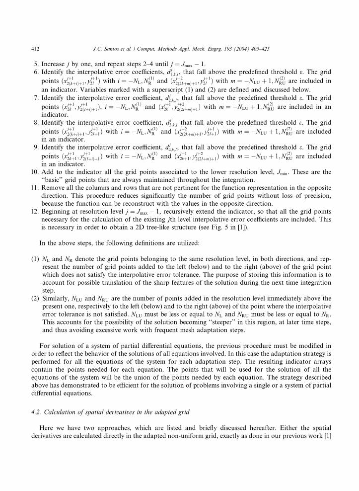
Fig. 5. Illustration of the calculation of the interpolating error coefficient, dj1;k;l.


5. Increase j by one, and repeat steps 2–4 until j ¼ Jmax � 1.

6. Identify the interpolative error coefficients, dj1;k;l, that fall above the predefined threshold e. The grid

points ðxjþ1

2ðkþiÞþ1; yjþ12l Þ with i ¼ �NL;N

ð1ÞR and ðxjþ2

2ð2kþmÞþ1; yjþ12l Þ with m ¼ �NLU þ 1;N ð2Þ

RU are included in

an indicator. Variables marked with a superscript (1) and (2) are defined and discussed below.

7. Identify the interpolative error coefficient, dj2;k;l, that fall above the predefined threshold e. The grid

points ðxjþ12k ; yjþ1

2ðlþiÞþ1Þ, i ¼ �NL;Nð1ÞR and ðxjþ1

2k ; yjþ2

2ð2lþmÞþ1Þ with m ¼ �NLU þ 1;N ð2ÞRU are included in an

indicator.

8. Identify the interpolative error coefficient, dj3;k;l that fall above the predefined threshold e. The grid

points ðxjþ1

2ðkþiÞþ1; yjþ12lþ1Þ with i ¼ �NL;N

ð1ÞR and ðxjþ2

2ð2kþmÞþ1; yjþ12lþ1Þ with m ¼ �NLU þ 1;N ð2Þ

RU are includedin an indicator.

9. Identify the interpolative error coefficient, dj4;k;l, that fall above the predefined threshold e. The grid

points ðxjþ12kþ1; y

jþ1

2ðlþiÞþ1Þ with i ¼ �NL;Nð1ÞR and ðxjþ1

2kþ1; yjþ2

2ð2lþmÞþ1Þ with m ¼ �NLU þ 1;N ð2ÞRU are included

in an indicator.

10. Add to the indicator all the grid points associated to the lower resolution level, Jmin. These are the

‘‘basic’’ grid points that are always maintained throughout the integration.

11. Remove all the columns and rows that are not pertinent for the function representation in the opposite

direction. This procedure reduces significantly the number of grid points without loss of precision,

because the function can be reconstruct with the values in the opposite direction.

12. Beginning at resolution level j ¼ Jmax � 1, recursively extend the indicator, so that all the grid points

necessary for the calculation of the existing jth level interpolative error coefficients are included. Thisis necessary in order to obtain a 2D tree-like structure (see Fig. 5 in [1]).

In the above steps, the following definitions are utilized:

(1) NL and NR denote the grid points belonging to the same resolution level, in both directions, and rep-

resent the number of grid points added to the left (below) and to the right (above) of the grid point

which does not satisfy the interpolative error tolerance. The purpose of storing this information is to

account for possible translation of the sharp features of the solution during the next time integrationstep.

(2) Similarly, NLU and NRU are the number of points added in the resolution level immediately above the

present one, respectively to the left (below) and to the right (above) of the point where the interpolative

error tolerance is not satisfied. NLU must be less or equal to NL and NRU must be less or equal to NR.

This accounts for the possibility of the solution becoming ‘‘steeper’’ in this region, at later time steps,

and thus avoiding excessive work with frequent mesh adaptation steps.

For solution of a system of partial differential equations, the previous procedure must be modified inorder to reflect the behavior of the solutions of all equations involved. In this case the adaptation strategy is

performed for all the equations of the system for each adaptation step. The resulting indicator arrays

contain the points needed for each equation. The points that will be used for the solution of all the

equations of the system will be the union of the points needed by each equation. The strategy described

above has demonstrated to be efficient for the solution of problems involving a single or a system of partial

differential equations.

4.2. Calculation of spatial derivatives in the adapted grid

Here we have two approaches, which are listed and briefly discussed hereafter. Either the spatial

derivatives are calculated directly in the adapted non-uniform grid, exactly as done in our previous work [1]


or, as a second alternative, the solution is interpolated to the maximum resolution level and the calculationsof the spatial derivatives are performed in that final uniform grid, as in [12]. The second approach is not

recommended as it involves too many unnecessary interpolations in the finest grid, in order to obtain the

values needed to calculate the spatial derivatives, thus leading to a tremendous slow down in the integration

process.

5. Application examples

In this section we present the results obtained in four test cases, designed to assess the accuracy and

robustness of the proposed strategy under different two-dimensional situations. We begin by solving the

classical linear advection equation. Then we solve the Smith–Hutton problem, which is a linear advection–

diffusion problem with a given velocity field, to show the ability of the method to deal with a spatially

varying velocity field with curved streamlines. In the third test case we solve the classical Burgers� equation,with and without viscosity, the prototypical non-linear transport equation. The final example is more

complex and consists on the solution of the system of Euler equations for gas dynamics: a coupled set of

four equations for the two Cartesian velocity components, density and pressure.All the calculations were performed in a 1.5 GHz Intel Pentium IV� personal computer with 1 GB of

RIMM memory.

5.1. Linear advection equation

This example considers the linear advection equation

ouot

¼ �aouox

�þ ou

oy

�ð15Þ

where, for convenience, the value of a ¼ 1 was adopted. The initial and boundary conditions correspond to

a classical benchmark problem of 2D-advection, and are given by

uðx; y; 0Þ ¼ 0;

uð0; y; tÞ ¼ 1; uðx; 0; tÞ ¼ 0:

The present test case has an exact solution represented by the transport, in space and time, of the unit

step u ¼ 1 applied at the left boundary (x ¼ 0), by the given velocity field, with equal unitary components

along the x and y co-ordinates. It thus offers a convenient means of assessing the performance of the

proposed adaptation strategy. A straightforward application of an unbounded discretization scheme, such

as central differencing or cubic splines, always conduces to the appearance of unphysical oscillations in thesolution, even with an extremely refined mesh, since the equation does not have a diffusive term. A bounded

method, such as the CUBISTA or MINMOD schemes presented in Section 2, introduces some artificial

diffusion in the vicinity of the step, if the mesh is not fine enough. Therefore an adaptive procedure is

needed in order to save memory and computational effort.

In this example there are, initially (for t6 1), two abrupt fronts: a step moving along the x-direction with

a velocity of a ¼ 1, and another moving along the x ¼ y-direction. For tP 1 there remains only one of the

fronts (along the main diagonal, x ¼ y). This means that for most of the integration time there are only two

localised regions where the mesh must be refined: one where the adaptation algorithm adds points only inthe x-direction (this happens for the step moving along the x-direction); and a region where addition of

points in both the x- and y-directions are needed (this happens with the front in x ¼ y).In this example the convection term was discretized with the MINMOD and CUBISTA high-resolution

schemes in the adapted non-uniform grid. Furthermore, it should be clear that, as in our previous work [1],

t0.0 0.2 0.4 0.6 0.8 1.0 1.2

no o

f gr

id p

oint

s (×

10-3

)

0

5

10

15

20

25

CUBISTAε = 10-3ε = 10-5

ε = 10-3

ε = 10-5

MINMOD

.

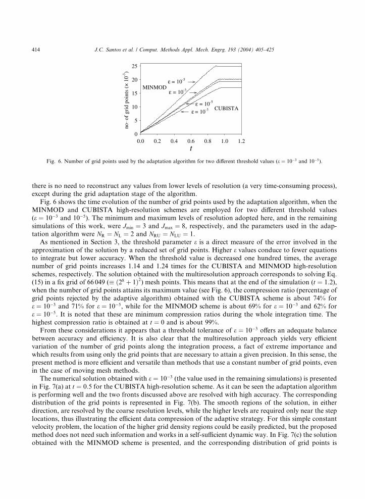
Fig. 6. Number of grid points used by the adaptation algorithm for two different threshold values (e ¼ 10�3 and 10�5).


there is no need to reconstruct any values from lower levels of resolution (a very time-consuming process),

except during the grid adaptation stage of the algorithm.

Fig. 6 shows the time evolution of the number of grid points used by the adaptation algorithm, when the

MINMOD and CUBISTA high-resolution schemes are employed for two different threshold values

(e ¼ 10�3 and 10�5). The minimum and maximum levels of resolution adopted here, and in the remaining

simulations of this work, were Jmin ¼ 3 and Jmax ¼ 8, respectively, and the parameters used in the adap-tation algorithm were NR ¼ NL ¼ 2 and NRU ¼ NLU ¼ 1.

As mentioned in Section 3, the threshold parameter e is a direct measure of the error involved in the

approximation of the solution by a reduced set of grid points. Higher e values conduce to fewer equations

to integrate but lower accuracy. When the threshold value is decreased one hundred times, the average

number of grid points increases 1.14 and 1.24 times for the CUBISTA and MINMOD high-resolution

schemes, respectively. The solution obtained with the multiresolution approach corresponds to solving Eq.

(15) in a fix grid of 66 049 (� ð28 þ 1Þ2) mesh points. This means that at the end of the simulation (t ¼ 1:2),when the number of grid points attains its maximum value (see Fig. 6), the compression ratio (percentage ofgrid points rejected by the adaptive algorithm) obtained with the CUBISTA scheme is about 74% for

e ¼ 10�3 and 71% for e ¼ 10�5, while for the MINMOD scheme is about 69% for e ¼ 10�3 and 62% for

e ¼ 10�5. It is noted that these are minimum compression ratios during the whole integration time. The

highest compression ratio is obtained at t ¼ 0 and is about 99%.

From these considerations it appears that a threshold tolerance of e ¼ 10�3 offers an adequate balance

between accuracy and efficiency. It is also clear that the multiresolution approach yields very efficient

variation of the number of grid points along the integration process, a fact of extreme importance and

which results from using only the grid points that are necessary to attain a given precision. In this sense, thepresent method is more efficient and versatile than methods that use a constant number of grid points, even

in the case of moving mesh methods.

The numerical solution obtained with e ¼ 10�3 (the value used in the remaining simulations) is presented

in Fig. 7(a) at t ¼ 0:5 for the CUBISTA high-resolution scheme. As it can be seen the adaptation algorithm

is performing well and the two fronts discussed above are resolved with high accuracy. The corresponding

distribution of the grid points is represented in Fig. 7(b). The smooth regions of the solution, in either

direction, are resolved by the coarse resolution levels, while the higher levels are required only near the step

locations, thus illustrating the efficient data compression of the adaptive strategy. For this simple constantvelocity problem, the location of the higher grid density regions could be easily predicted, but the proposed

method does not need such information and works in a self-sufficient dynamic way. In Fig. 7(c) the solution

obtained with the MINMOD scheme is presented, and the corresponding distribution of grid points is

Fig. 7. (a) Solution at t ¼ 0:5 of the linear advection equation with a step profile for the CUBISTA scheme and (b) corresponding

distribution of grid points in terms of spatial location. (c) Solution for the MINMOD scheme and (d) corresponding distribution of

grid points in terms of spatial location.


illustrated in Fig. 7(d). As can be observed, the solution computed with the MINMOD scheme is less

accurate despite using a higher number of grid points. This illustrates the superiority of the CUBISTA

scheme in terms of accuracy.

The same problem was also solved on equivalent uniform meshes having ð2Jmax þ 1Þ2 grid points, with the

aim of calculating the increase rate of grid points in the adaptive approach, the CPU time and the speed-up

factors, defined as the ratio of CPU times for the uniform mesh and the adaptive calculations. Here Jmax

was varied from 3 up to 10.

The increase rate of grid points (IRGP), defined as the ratio between the number of grid points used intwo consecutive resolution levels for the adaptive approach, is presented in Table 1. In a uniform mesh this

number tends to 4 while in the adaptive approach tends to 2.3 for both the MINMOD and CUBISTA

schemes, as it can be seen in Table 1. This means that, for high levels of resolution, when passing from one

level to the next one, the CPU time should increase 4.6 times (¼ 2.3 · 2, where the factor 2 results from the

necessity of halving the time step, even for a variable time-step solver such as LSODA) using the adaptation

Table 1

Number of grid points (NGP), compression ratio (CR) and increase rate of grid points (IRGP) for the linear advection equation, using

the adaptive approach

Jmax Uniform

mesh

Adaptive mesh

MINMOD CUBISTA

NGP NGP IRGP CR (%) NGP IRGP CR (%)

3 81 81 – 0.0 81 – 0.0

4 289 234 2.89 19.0 215 2.65 25.6

5 1089 549 2.35 49.6 486 2.26 55.4

6 4225 1172 2.13 72.3 1017 2.09 75.9

7 16 641 2524 2.15 84.8 2179 2.14 86.9

8 66 049 5547 2.20 91.6 4 754 2.18 92.8

9 263 169 12 456 2.25 95.3 10 589 2.23 96.0

10 1 050 625 28 380 2.28 97.3 23 710 2.24 97.7

The values correspond to the average from t ¼ 0 to t ¼ 0:5.

Table 2

Speed-up factors and CPU times for the linear advection equation (t ¼ 0:5) calculated with the CUBISTA scheme

Jmax Uniform mesh Adaptive mesh

NGPa CPU (s) NGPa CPU (s) Speed-up

3 81 0.48 81 0.48 1.00

4 289 2.74 283 2.24 1.22

5 1089 16.99 732 9.12 1.86

6 4225 117.78 1725 41.76 2.82

7 16 641 855.42 4036 204.92 4.17

aNumber of grid points. For the adaptive strategy, values are the average from t ¼ 0 to 0.5.


algorithm and 8 times, using a uniform mesh. From this analysis, the maximum theoretical rate of increase

of the speed-up factors that can be obtained with the present approach is about 1.7 (¼ 8/4.6). It is inter-

esting to note that the IRGP tends to the same value, as Jmax increases, irrespective of being calculated

based on the instantaneous number of grid points, or the average value from t ¼ 0 (not shown in Table 1).

Table 2 presents the speed-up factors and CPU times for uniform and adaptive mesh approaches. The

CPU times were calculated only for resolution levels up to seven, because, for higher values, the calcula-tions with the uniform mesh approach required more physical computer memory than available. In this

situation, virtual memory would be needed and that would distort the CPU time comparison.

The calculated speed-up factors increase exponentially with mesh refinement (almost at the rate of 1.7, as

discussed before), and can be as high as we want.

From the previous tests we found that the CUBISTA scheme is more accurate and the speed-up factors

are higher than those for the MINMOD scheme (due to the use of less grid points to attain a given pre-

cision). This is why, in the following examples, the CUBISTA scheme was selected for all the calculations.

5.2. Smith–Hutton problem

This example considers the Smith–Hutton test problem, described by the following convection–diffusion

equation [16]:

oTot

¼ 1

Peo2Tox2

�þ o2T

oy2

�� oðaxT Þ

ox

�þ oðayT Þ

oy

�; ð16Þ


where Pe is the Peclet number, T is the temperature (the unknown variable in this case) and ax and ay are thevelocity components in the x- and y-directions respectively. A difference with the previous test case is that

now the velocity field is non-uniform, varying from point to point, and corresponds to curved streamlines

with Cartesian velocity components defined as

ax ¼ 2yð1� x2Þ; ay ¼ �2xð1� y2Þ: ð17ÞThe problem was solved for two values of the Peclet number, which measures the strength of convection

in relation to diffusion, namely Pe ¼ 500 (moderate convection) and Pe ! 1 (convection dominated flow).

The solution domain is �16 x6 1 and 06 y6 1, and the following initial and boundary conditions were

applied, as used by Darwish and Moukalled in [17]:

T ðx; y; 0Þ ¼ 0;

T ð�1; y; tÞ ¼ 0; T ð1; y; tÞ ¼ 0;

T ðx; 1; tÞ ¼ 0; T ðx; 0; tÞ ¼ 1 � 0:56 x6 0;0 elsewhere:

�

Physically, the problem can be described as follows: the temperature is initially zero everywhere and a

step profile is imposed along the negative side of the x-axis (T ¼ 0, x < �1=2; T ¼ 1, xP � 1=2), this‘‘step’’ is then convected by the circular velocity field, from the left quadrant (x6 0) to the right one (x > 0).

The computed solution with the CUBISTA high-resolution scheme is presented in Fig. 8(a) at t ¼ p=4, forPe ! 1. Similarly to the previous example, the use of an unbounded discretization scheme always leads to

the appearance of unphysical oscillations in the solution, since the equation does not have a diffusive term

(where Pe ! 1). The application of a high-resolution scheme is therefore imposed. The distribution of the

grid points is represented in Fig. 8(b). Note that the smooth regions of the solution are resolved by a low

density of grid points while high density is only required near the front location, thus illustrating the

efficient data compression of the adaptive strategy.

Fig. 9(a) shows the solution at the same simulation time, t ¼ p=4, for the case when some diffusion is

present, Pe ¼ 500. The purpose of this test case is to demonstrate the ability of the proposed method to dealwith problems having a diffusive term. An unbounded discretization scheme could, in principle, be used,

but in order to avoid the appearance of unphysical oscillations, the mesh would have to be extremely re-

fined in the vicinity of the sharp, curved fronts. Our algorithm is however more general and can be used in

both situations, as can be seen by the correct location of grid points in Fig. 9(b).

The number of grid points used by the adaptation algorithm with Pe ! 1 and Pe ¼ 500 is presented in

Fig. 10. The evolution is similar to Fig. 6, but now the increase of the number of grid points is not linear

with simulation time. Once again the adaptive strategy is performing well, and the compression ratios at the

end of the simulation are 78% and 81% for Pe ! 1 and Pe ¼ 500, respectively.

Fig. 8. (a) Solution of the Smith–Hutton problem at t ¼ p=4 with Pe ! 1 and (b) corresponding distribution of grid points in terms of

spatial location.

Fig. 9. (a) Solution of the Smith–Hutton problem at t ¼ p=4 with Pe ¼ 500 and (b) corresponding distribution of grid points in terms

of spatial location.

t0 1 2 3

no o

f gr

id p

oint

s (×

10-3

)

0

2

4

6

8

10

12

14

16

Pe = 500

Pe = ∞

.

Fig. 10. Number of grid points used by the adaptation algorithm for the Smith–Hutton problem.

Table 3

Number of grid points (NGP), compression ratio (CR) and increase rate of grid points (IRGP) for the Smith–Hutton test problem for

Pe ! 1, using the adaptive approach


NGP NGP IRGP CR (%)

3 81 81 – 0.0

4 289 239 2.95 17.3

5 1089 547 2.29 49.8

6 4225 1234 2.26 70.8

7 16 641 2879 2.33 82.7

8 66 049 6896 2.40 89.6

9 263 169 16 392 2.38 93.8

10 1 050 625 38 317 2.34 96.4

The values correspond to the average from t ¼ 0 to p=4.


Table 3 presents the increase rate of grid points (IRGP), defined as the ratio between the number of gridpoints used in two consecutive resolution levels for the adaptive approach. As in the previous problem the

increase rate of grid points when using the adaptive strategy tends to 2.3 in contrast with the value of 4

obtained with a uniform mesh.


5.3. Burgers’ equation

This example considers the numerical solution of the classical Burgers� equation [18]:

ouot

¼ to2uox2

�þ o2u

oy2

�� of ðuÞ

ox

�þ of ðuÞ

oy

�; ð18Þ

where the flux is f ðuÞ ¼ u2=2. Here u may be taken as a velocity (or other advected property), x and y are

the spatial co-ordinates, t is the time variable and t is the viscosity. All variables are normalized and so tmay be considered as the inverse of a Reynolds number.

This equation is frequently used for testing numerical methods since it is non-linear and consequently,

depending of the initial conditions chosen, discontinuities may develop from smooth solutions [19].

Eq. (18) was solved in the domain �1:56 x6 1:5 and �1:56 y6 1:5, with either t ¼ 5:0� 10�3 or in theinviscid limit (t ! 0), and the following initial and boundary conditions were applied, following Kurganov

and Tadmor [20]:

uðx; y; 0Þ ¼�1 ðx� 0:5Þ2 þ ðy � 0:5Þ2 6 0:42;

1 ðxþ 0:5Þ2 þ ðy þ 0:5Þ2 6 0:42;

0 elsewhere;

8><>:

uð�1:5; y; tÞ ¼ 0; uð1:5; y; tÞ ¼ 0; uðx;�1:5; tÞ ¼ 0; uðx; 1:5; tÞ ¼ 0:

For this specific type of initial condition there will be two cylindrical fronts which move with velocities

equal to the mean of the velocities just before and after the shock front, while the trailing edges do not move

at all. After a certain time gap (t � 0:307 for t ¼ 0) the fronts will touch each other and will form a dis-

continuity in the solution, since they move in opposite directions; note that the cylinder centered in the third

quadrant of the xy plane has a positive velocity. The velocity distributions at t ¼ 0:5 and 2, considering the

inviscid limit, are presented in Fig. 11(a) and (b) respectively. The corresponding distribution of the grid

points for t ¼ 0, 0.5 and 2 are shown in Fig. 11(c)–(e), respectively.When a small amount of ‘‘viscosity’’ is added to the equations the main features of the solution remain

unchanged, except for the larger region in the original domain which is affected by the initial distribution of

u. Now the trailing edges of the initial cylindrical distributions do move away from the centres due to

transport by diffusion. For this case the velocity distributions at t ¼ 0:5 and 2, with t ¼ 5:0� 10�3, are

presented in Fig. 12(a) and (b) respectively. The distribution of the grid points for t ¼ 0:5 and 2 is presented

in Fig. 12(c) and (d), respectively. The adaptation strategy proves to be capable of dealing with highly non-

linear equations that include diffusive terms, as seen by the correct allocation of the grid points shown in

Fig. 12(d).Fig. 13 shows the time evolution of the number of grid points used by the adaptation algorithm. It is

interesting to note that, for t ¼ 5:0� 10�3, at t � 0:8 the number of grid points needed to compute the

solution, with the prescribed threshold of e ¼ 10�3, decreases significantly. This result is very important

since it demonstrates a virtue of the current strategy as compared to other approaches, such as the moving

mesh method, where a constant number of grid points are used throughout the computations. The pro-

posed strategy uses only the grid points that are actually necessary to attain a given precision, and so is

more versatile and efficient.

Table 4 presents the increase rate of grid points (IRGP), defined as the ratio between the number ofgrid points used in two consecutive resolution levels for the adaptive approach. For this problem the

tendency of the increase rate of grid points when using the adaptive strategy is still not very well defined at

Jmax ¼ 10.

Fig. 11. Solution of the Burgers� equation, without viscosity (t ¼ 0), at (a) t ¼ 0:5 and (b) t ¼ 2. Distribution of grid points in terms of

spatial location at (c) t ¼ 0, (d) t ¼ 0:5 and (e) t ¼ 2.


Fig. 12. Solution of the Burgers� equation with t ¼ 5:0� 10�3 at (a) t ¼ 0:5 and (b) t ¼ 2. Distribution of grid points in terms of spatial

location at (c) t ¼ 0:5 and (d) t ¼ 2.

t0.0 0.5 1.0 1.5 2.0

no o

f gr

id p

oint

s (×

10-3

)

12

14

16

18

20

22

υ = 0

υ = 5×10-3

.

Fig. 13. Number of grid points used by the adaptation algorithm for the solution of the Burgers� equation.


Table 4

Number of grid points (NGP), compression ratio (CR) and increase rate of grid points (IRGP) for the Burgers� equation for t ¼ 0,

using the adaptive approach


NGP NGP IRGP CR (%)

3 81 81 – 0.0

4 289 269 3.32 6.9

5 1089 806 3.00 26.0

6 4225 2349 2.91 44.4

7 16 641 6567 2.80 60.5

8 66 049 17 273 2.63 73.8

9 263 169 43 296 2.51 83.5

10 1 050 625 111 381 2.57 89.4

The values correspond to the average from t ¼ 0 to 2.


5.4. Compressible Euler system

In this final example we test the proposed adaptive strategy on a problem involving the 2D compressible

Euler system of conservation laws for gas dynamics, which is written in conservative form as follows:

o

ot

qquqvE

2664

3775þ o

ox

ququ2 þ pquv

uðE þ pÞ

2664

3775þ o

oy

qvquv

qv2 þ pvðE þ pÞ

2664

3775 ¼ 0; ð19Þ

where q, u, v and E are the density, x- and y-velocities and total energy of the gas per unit volume,

respectively. The pressure, p, is given by

p ¼ ðc� 1Þ Eh

� q2ðu2 þ v2Þ

i; ð20Þ

where c is the ratio of specific heats (c ¼ 1:4 is a good approximation for air). We solved the benchmark

Riemann problem inspired by the standard 1D Sod shock-tube problem, which consists of the initial data(as in Configuration 4 of [21]):

pq

uv

2666437775ðx; y; 0Þ ¼

½ 1:1 1:1 0 0 �T x > 0:5; y > 0:5;

½ 0:35 0:5065 0:8939 0 �T x < 0:5; y > 0:5;

½ 1:1 1:1 0:8939 0:8939 �T x < 0:5; y < 0:5;

½ 0:35 0:5065 0 0:8939 �T x > 0:5; y < 0:5:

8>>><>>>:

At x ¼ 0, x ¼ 1, y ¼ 0 and y ¼ 1 reflecting boundary conditions are imposed. Several approaches can be

found in the literature for the solution of Euler system of equations, either in the context of Riemann

solvers [22] or pressure-based algorithms [23]. In this work we selected the semi-discrete central scheme of

Kurganov and Tadmor [20], which is an extension to higher-order accuracy of the well-known Lax–

Friedrichs scheme [24]. This semi-discrete central scheme requires the use of a TVD limiter in order to

prevent formation of unphysical oscillations in the solution. It is here that the recently developed CUBI-

STA scheme [7], explained in Section 2, shows its potential because it was devised in such a way that TVDconditions are satisfied.

Results for the gas density distribution and the corresponding location of grid points at times t ¼ 0, 0.1

and 0.2 are presented in Fig. 14. The propagation of several fronts is seen to be well represented, with very

sharp resolution, and the interaction region does not show signs of spurious oscillations in the computed

fields.

Fig. 14. Solution for the gas density of the compressible Euler system at (a) t ¼ 0:1 and (b) t ¼ 0:2. Distribution of grid points in terms

of spatial location at (c) t ¼ 0, (d) t ¼ 0:1 and (e) t ¼ 0:2.



6. Conclusions

A multiresolution approach for solving the typical PDEs of mathematics/physics has been described and

applied to a number of two-dimensional test cases. Key features of this approach are the mesh adaptation

strategy, whereby high density of grid points is allocated only where it is needed, and the high-resolution

scheme for the convection terms, which prevents the formation of unphysical oscillations near sharp fronts.

The examples presented have demonstrated that the multiresolution approach can resolve very accu-

rately the various moving fronts present in the solutions, for both linear and non-linear problems, involvingeither a single or a system of equations, while the total number of grid points required to achieve such level

of resolution was seen to increase only moderately with the simulation time and the number of grid levels.

In fact, compared with a fixed grid approach, in which grid doubling leads to 4 times more grid points, for

the multiresolution approach the factor was found to be between 2.3 and 2.5. As a consequence the speed-

up factor (ratio of CPU time for uniform mesh/adaptive mesh) was seen for the examples to increase at a

rate almost around 1.7 as the level of resolution increases. Therefore, these speed-up factors quickly attain

very high values; we found a typical value of 4.2 for a resolution level of 7 (which is fairly typical in current

applications). These figures illustrate the efficiency of the proposed adaptive multiresolution approach.

Acknowledgements

The work of J.C. Santos and P. Cruz was supported by FCT (grants SFRH/BD/6817/2001 and BD/

21483/99, respectively). M.A. Alves wishes to thank the financial support provided by Fundac�~aao Calouste

Gulbenkian.

References

[1] M.A. Alves, P. Cruz, A. Mendes, F.D. Magalh~aaes, F.T. Pinho, P.J. Oliveira, Adaptive multiresolution approach for solution of

hyperbolic PDEs, Comput. Methods Appl. Mech. Engrg. 191 (2002) 3909–3928.

[2] S. Mallat, Multiresolution approximation and wavelet orthogonal bases of L2ðRÞ, Trans. Amer. Math. Soc. 315 (1989) 69–87.

[3] A. Harten, Multiresolution representation of data: a general framework, SIAM J. Numer. Anal. 33 (1996) 1205–1256.

[4] A. Harten, B. Engquist, S. Osher, S.R. Chakravarthy, Uniformly high order accurate essentially non-oscillatory schemes III, J.

Comput. Phys. 71 (1987) 231–303.

[5] A. Cohen, S.M. Kaber, S. Muller, M. Postel, Fully adaptive multiresolution finite volume schemes for conservation laws, Math.

Comput. 72 (2003) 183–225.

[6] S. Karni, A. Kurganov, G. Petrova, A smoothness indicator for adaptive algorithms for hyperbolic systems, J. Comput. Phys. 178

(2002) 323–341.

[7] M.A. Alves, P.J. Oliveira, F.T. Pinho, A convergent and universally bounded interpolation scheme for the treatment of advection,

Int. J. Numer. Methods Fluids 41 (2003) 47–75.

[8] B.P. Leonard, The Ultimate conservative difference scheme applied to unsteady one-dimensional advection, Comput. Methods.

Appl. Mech. Engrg. 88 (1991) 17–74.

[9] B.P. Leonard, Bounded higher-order upwind multidimensional finite-volume convection–diffusion algorithms, in: W.J.

Minkowycz, E.M. Sparrow (Eds.), Advances in Numerical Heat Transfer, vol. 1, Taylor and Francis, 1996, pp. 1–57.

[10] M.S. Darwish, F.H. Moukalled, Normalized variable and space formulation methodology for high-resolution schemes, Numer.

Heat Transfer B 26 (1994) 79–96.

[11] A. Harten, High resolution schemes for hyperbolic conservation laws, J. Comput. Phys. 49 (1983) 357–393.

[12] M. Holmstr€oom, Solving hyperbolic PDEs using interpolating wavelets, SIAM J. Sci. Comput. 21 (1999) 405–420.

[13] J. Walden, Filter bank methods for hyperbolic PDEs, SIAM J. Numer. Anal. 36 (1999) 1183–1233.

[14] H.-M. Zhou, Wavelet transforms and PDE techniques in image compression, Ph.D. Thesis, Department of Mathematics, UCLA,

2000.

[15] L.R. Petzold, Automatic selection of methods for solving stiff and nonstiff systems of ordinary differential equations, SIAM J. Sci.

Statist. Comput. 4 (1983) 136–148.


[16] B.P. Leonard, J.E. Drummond, Why you should not use �Hybrid�, �Power law� or related exponential schemes for convective

modelling––There are much better alternatives, Int. J. Numer. Methods Fluids 20 (1995) 421–442.

[17] M.S. Darwish, F. Moukalled, TVD schemes for unstructured grids, Int. J. Heat Mass Transf. 46 (2003) 599–611.

[18] C.A.J. Fletcher, Computational Techniques for Fluid Dynamics, vol. I, second ed., Springer-Verlag, Berlin, 1991.

[19] N.N. Carlson, K. Miller, Design and application of a gradient-weighted moving finite element code I: in one dimension, SIAM J.

Sci. Comput. 19 (1998) 728–765.

[20] A. Kurganov, E. Tadmor, New high-resolution central schemes for nonlinear conservation laws and convection–diffusion

equations, J. Comput. Phys. 160 (2000) 241–282.

[21] A. Kurganov, E. Tadmor, Solution of two-dimensional Riemann problems for gas dynamics without Riemann problem solvers,

Numer. Methods Partial Differential Equations 18 (2002) 584–608.

[22] C. Hirsch, in: Numerical Computation of Internal and External flows, vol. 2, John Wiley, Chichester, 1990.

[23] J.H. Ferziger, M. Peri�cc, Computational Methods for Fluid Dynamics, Springer-Verlag, Berlin, 1996.

[24] P.D. Lax, Weak solutions of nonlinear hyperbolic equations and their numerical computation, Comm. Pure Appl. Math. 7 (1954)

159–193.

Adaptive multiresolution approach for two-dimensional PDEs

Documents

Transcript of Adaptive multiresolution approach for two-dimensional PDEs