A scale space multiresolution method for extraction of time series features

StatThe ISI’s Journal for the Rapid (wileyonlinelibrary.com) DOI: 10.1002/sta4.35Dissemination of Statistics Research

A scale space multiresolution method forextraction of time series featuresLeena Pasanena, Ilkka Launonena and Lasse Holmströma

Received 8 October 2013; Accepted 19 October 2013

A scale space multiresolution feature extraction method is proposed for time series data. The method detectsintervals where time series features differ from their surroundings, and it produces a multiresolution analysis of theseries as a sum of scale-dependent components. These components are obtained from differences of smooths. Therelevant sequence of smoothing levels is determined using derivatives of smooths with respect to the logarithm ofthe smoothing parameter. As time series are usually noisy, the method uses Bayesian inference to establish thecredibility of the components. © The Authors. Stat published by John Wiley & Sons Ltd.

Keywords: Bayesian methods; simulation; smoothing; time series; visualization

1 IntroductionA typical aim of nonparametric regression is to estimate the signal from noisy data by smoothing, where the smooth-ness of the estimate is controlled by a smoothing parameter. The fundamental question then is, which level ofsmoothing uncovers the signal best, revealing such features as local minima and maxima. The aim of scale spaceanalysis differs from this by viewing the signal on several smoothing scales, all of which are considered to containvaluable information about the data, instead of finding a single best fit.

Scale space analysis was made popular in computer vision literature by Lindeberg (1994). It was later introduced tostatistics by Chaudhuri & Marron (1999, 2000) in the form of the significant zero crossings of the derivative (SiZer)method, which detects statistically significant increasing or decreasing intervals from nonparametric regression curvesor density estimates on several scales. Later, a Bayesian SiZer (BSiZer) was proposed by Erästö & Holmström (2005).A different Bayesian approach was proposed by Godtliebsen & Øigård (2005). For reviews of statistical scale spacemethods and BSiZer, see Holmström (2010b, 2010a), respectively.

Let �, y 2 Rn and S� 2 Rn�n be the underlying signal, the observed noisy series and a smoothing operator corre-sponding to a smoothing level � > 0, respectively, and let ¹�iº be an increasing sequence of smoothing levels. TheSiZer and BSiZer analyses produce a map that consists of pixels .i, j/ where i is the scale index and j is the time index.The ith row of the map corresponds to the time derivative of the smooth S�i�. The color of the pixel .i, j/ depends onthe sign of the derivative. To determine the pixel color, SiZer applies frequentist statistical methods to the observed y,whereas BSiZer uses the posterior distribution p.�jy/.

aDepartment of Mathematical Sciences, University of Oulu, P.O. Box 3000, 90014 Oulu, Finland∗Email: [email protected] is an open access article under the terms of the Creative Commons Attribution Non-Commercial License, which permitsuse, distribution and reproduction in any medium, provided the original work is properly cited and is not used for commercialpurposes.

Stat 2013; 2: 273–291 © The Authors. Stat published by John Wiley & Sons Ltd

http://creativecommons.org/licenses/by-nc/3.0/

https://www.researchgate.net/publication/229799576_Scale_space_methods?el=1_x_8&enrichId=rgreq-27be5aa1-5d97-4bee-8f50-a896f9a057f3&enrichSource=Y292ZXJQYWdlOzI1OTU0MzAxMDtBUzo5OTAzMzM0MzMzMjM3OUAxNDAwNjIyNzk3OTY4

L. Pasanen et al. Stat(wileyonlinelibrary.com) DOI: 10.1002/sta4.35 The ISI’s Journal for the Rapid

Dissemination of Statistics Research

Here, we take a different approach to time series feature extraction. Instead of detecting intervals where the derivativeis credibly positive or negative, we detect intervals where the values of � are higher or lower than its average in alocal neighborhood and construct a multiresolution analysis of � as a sum of scale-dependent components. This isaccomplished by considering differences of smooths. In Holmström et al. (2011), such an approach was used fordigital images. In practice, first a sample is drawn from the posterior distribution of �, and then, posterior samples ofthe scale-dependent components are obtained by applying a difference of smooths operator S�i � S�j , where �i < �j,to this sample. The credibly nonzero intervals of the components are then detected.

The smoothing levels used to compute the differences of smooths must be carefully chosen to correctly extract thecomponents in the signal. For this, a scale-derivative map resembling SiZer and BSiZer maps is used (e.g., bottompanel of Figure 1). However, in contrast to SiZer and BSiZer, which consider the time derivative of the smoothed signal,each row i of the scale-derivative map corresponds to the derivative of the smooth S�� with respect to log� computedat �i, where log denotes the natural logarithm. A column j measures how the intensity of the smooth changes as afunction of the scale at time j. The values �i used in the final multiresolution analysis are the values that correspondto the rows of this map where the derivative is uniformly close to zero. Because � is unknown, we use the posteriormean of � to calculate the derivative of the smooth.

The difference of smooths is familiar also in image analysis literature, where it is used as an edge detection method.This is based on the fact that the edges of features are located at the zero crossings of the Laplace operator, which,by the heat equation, can be approximated by the less computationally intensive difference of Gaussian smooths(Marr & Hildreth, 1980). As we are dealing with one-dimensional data, differences of smooths can be used as anapproximation of the second time derivative. SiZer and BSiZer detect local maxima and minima as zero crossingsof the derivative, whereas here, in the spirit of edge detection, zero crossings of the second derivative correspond tointensity changes.

The article is organized as follows. Section 2.1. presents the idea of a scale space multiresolution analysis. Theselection of smoothing levels and the scale-derivative map are discussed in Section 2.2.. Section 2.3. introducescredibility analysis for noisy data. Section 3 presents analyses of real and artificial time series, considers the rate offalse-positives by analyzing samples from Gaussian noise and makes comparison with other SiZer-related methods.We conclude the article with a discussion in Section 4. A MATLAB implementation of the method is available onlineat http://cc.oulu.fi/~lpasanen/MRBSiZer1D/.

2 Bayesian multiresolution analysis of time series2.1. A multiresolution decompositionConsider a signal � D[�1, : : : ,�n]T observed at times t1 < t2 < � � � < tn. We try to decompose � into scale-dependent components obtained from differences S�i� � S�iC1� of smooths determined by an appropriate choice ofthe smoothing parameter sequence ¹�iº.

For smoothing, we use a discrete spline smoother

S� D .IC �CTC/�1, (1)

where C 2 R.n�2/�n is the second-order difference matrix, that is, Cp D w with

wj DpjC2 � pjC1

tjC2 � tjC1�

pjC1 � pj

tjC1 � tj, j D 1, : : : , n � 2. (2)

As �!1, S�� converges to the linear regression line.

© The Authors. Stat published by John Wiley & Sons Ltd 274 Stat 2013; 2: 273–291

http://cc.oulu.fi/~lpasanen/MRBSiZer1D/

https://www.researchgate.net/publication/220055949_Scale_space_multiresolution_analysis_of_random_fields?el=1_x_8&enrichId=rgreq-27be5aa1-5d97-4bee-8f50-a896f9a057f3&enrichSource=Y292ZXJQYWdlOzI1OTU0MzAxMDtBUzo5OTAzMzM0MzMzMjM3OUAxNDAwNjIyNzk3OTY4

Stat Multiresolution analysis of time series

The ISI’s Journal for the Rapid (wileyonlinelibrary.com) DOI: 10.1002/sta4.35Dissemination of Statistics Research

The smoothing operator S� can be thought of as a low-pass filter. Hence, the difference of smooths S�i � S�j , with�i < �j, can be thought of as a bandpass filter that isolates features that are present at level �i but not at �j (Holmströmet al., 2011). Let

0 D �1 < �2 < � � � < �L�1 < �L � 1

be a sequence of smoothing levels and denote the mean of � by N�. Because S�1� D �, we can decompose � into

components as

� D

L�1XiD1

.S�i � S�iC1/�C S�L� � N�1C N�1 �LC1XiD1

zi, (3)

where zi D .S�i � S�iC1/� for i D 1, : : : , L � 1, zL D SL� � N�1 and zLC1 D N�1. The component zi can be interpreted

as the detail of � which is smoothed out when smoothing is increased from �i to �iC1. If �L D 1, zL correspondsto the linear trend. It follows easily from the properties of the smoother (1) that z1, : : : , zL�1 have no linear trend andNzi D 0, except for zLC1 (cf. section 2.1 in Erästö & Holmström, 2005).

For exploratory purposes, such analysis can be performed directly on the actual observed noisy series y. In this case,the noise may be possible to filter out as the smallest-scale component. Figure 5 shows a scale-derivative map andscale-dependent components for raw data. However, in order to make inferences about the underlying structures of theseries, the posterior distribution of � is used instead. Given a sample from the distribution p.�jy/, we make inferencesabout the credibility of the scale-derivative map and the scale-dependent components. The inference is summarizedin the form of maps and displays that use white, black and gray to indicate properties of the derivative and the signalcomponents. The right panel of Figure 8 shows an example of inference for a scale-derivative map, and Figure 9shows inference for scale-dependent components.

2.2. The scale-derivative map and the selection of smoothing levelsTo achieve a good separation of the scale-dependent components, the sequence ¹�iº in (3) needs to be chosencarefully. Intuitively, the idea is as follows. Consider a signal � D

PLC1iD1 �i that consists of a sum of components �i of

different scales, ordered according to ascending magnitude of the scale, where �1 is the smallest-scale component.We assume that �i has no linear trend for i D 1, : : : , L� 1 and N�i D 0 except for the constant vector �LC1. We shouldthen find a sequence ¹�iº for which zi D .S�i � S�iC1/� � �i, i D 1, : : : , L� 1. This is possible because the smootherS� acts as a low-pass filter. Therefore, for each k D 1, : : : , L, there is a smoothing level �k for which

S�k� �

LC1XiDk

�i,

if the scales of the components are sufficiently distinct. Thus, .S�k � S�kC1/� � �k for k D 1, : : : , L � 1.

A principled method for choosing suitable smoothing levels �i can be based on the derivative of the smooth S��with respect to log�. The logarithmic scale for � is preferable because the larger the smoothing levels, the larger thedistance between successive values of � has to be to have a noticeable effect on the smooth. The derivative is

D�� D lim�0!�

S�0� � S��log�0 � log�

D ��.IC �CTC/�1CTC.IC �CTC/�1�.

We pick the values �2, : : : ,�L as the local minima of the norm kD��k (e.g., Figure 2). This can be justified as follows.

Consider a signal � that consists of only one component with no linear trend and zero mean. Because of the low-passnature of the smoother S�, the signal remains nearly unaltered for a sufficiently small �0, that is, S�� for � � �0.

Stat 2013; 2: 273–291 275 © The Authors. Stat published by John Wiley & Sons Ltd



For a sufficiently large smoothing level �00, the signal will be close to zero for � � �00. Then, kD��k is close to zero forboth � � �0 and � � �00. If � is a sum of two zero-mean components �1 and �2 with sufficiently distinct scales, where�1 has no linear trend, there is a smoothing level �0 for which the smaller-scale component is mostly smoothed outbut which doesn’t affect the larger-scale component. Therefore, �0 is a local minimum of kD��k and �� S�0� � �1,S�0� � �2. Similarly, assuming sufficient separation of successive scales, � D

PLC1iD1 �i can be decomposed using

the L � 1 local minima of kD��k.

The derivative D�� itself also provides detailed information about the features of � at different time points. Theinformation is visualized using the scale-derivative map, where the color of the pixel .i, j/ corresponds to the jthelement of the vector D�i�. A suitable sequence of smoothing parameters can be searched also visually from thescale-derivative map by looking for rows where the derivative is uniformly close to zero between strongly colored areas.This may be necessary, for example, when a component has a variable scale with respect to time (cf. Section 3.3.).It is then broken into several subcomponents with a fixed scale over some time intervals while being nearly constantelsewhere. Close inspection of the scale-derivative map is also recommended when the data are highly nonequispaced.

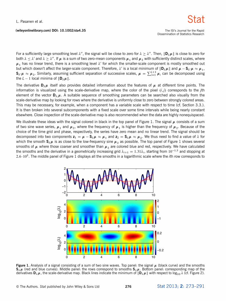
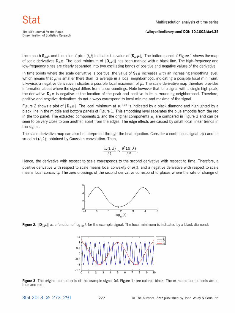
We illustrate these ideas with the signal colored in black in the top panel of Figure 1. The signal � consists of a sumof two sine wave series, �1 and �2, where the frequency of �1 is higher than the frequency of �2. Because of thechoice of the time grid and phase, respectively, the series have zero mean and no linear trend. The signal should bedecomposed into two components z1 D � � S�� 1 and z2 D S�� 2. We thus need to find a value of � forwhich the smooth S�� is as close to the low-frequency sine �2 as possible. The top panel of Figure 1 shows severalsmooths of � where those coarser and smoother than �2 are colored blue and red, respectively. We have calculatedthe smooths and the derivative in a geometrically increasing grid �iC1 D 1.31�i, starting from 10�1.5 and stopping at2.6 �105. The middle panel of Figure 1 displays all the smooths in a logarithmic scale where the ith row corresponds to

−2

−1

0

1

2

log 10

(λ)

log 10

(λ)

0 2 4 6 8 10

0 2 4 6 8 10

0 2 4 6 8 10

0

2

4

−1

0

1

2

0

2

4

−0.2

0

0.2

Figure 1. Analysis of a signal consisting of a sum of two sine waves. Top panel: the signal � (black curve) and the smoothsS�� (red and blue curves). Middle panel: the rows correspond to smooths S��. Bottom panel: corresponding map of thederivatives D��, the scale-derivative map. Black lines indicate the minimum of kD��k with respect to log10 � (cf. Figure 2).




the smooth S�i� and the color of pixel .i, j/ indicates the value of .S�i�/j. The bottom panel of Figure 1 shows the mapof scale derivatives D��. The local minimum of kD��k has been marked with a black line. The high-frequency andlow-frequency sines are clearly separated into two oscillating bands of positive and negative values of the derivative.

In time points where the scale derivative is positive, the value of S�� increases with an increasing smoothing level,which means that � is smaller there than its average in a local neighborhood, indicating a possible local minimum.Likewise, a negative derivative indicates a possible local maximum of �. The scale-derivative map therefore providesinformation about where the signal differs from its surroundings. Note however that for a signal with a single high peak,the derivative D�� is negative at the location of the peak and positive in its surrounding neighborhood. Therefore,positive and negative derivatives do not always correspond to local minima and maxima of the signal.

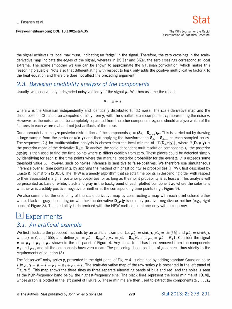
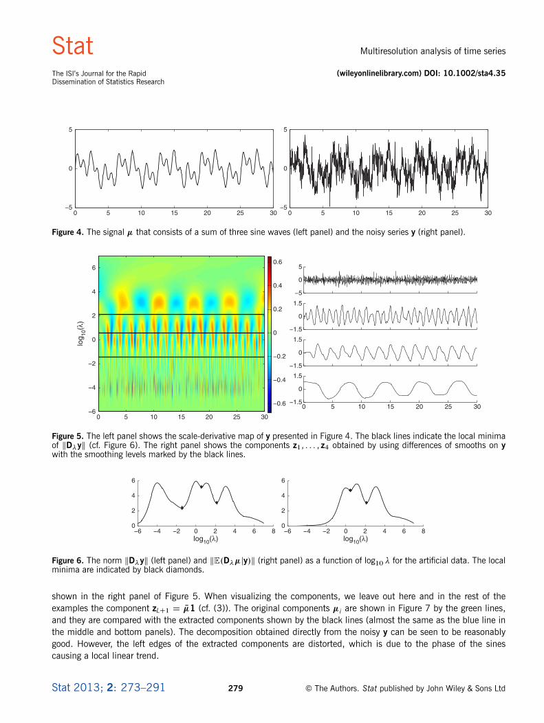
Figure 2 shows a plot of kD��k. The local minimum at 101.78 is indicated by a black diamond and highlighted by ablack line in the middle and bottom panels of Figure 1. This smoothing level separates the blue smooths from the redin the top panel. The extracted components zi and the original components �i are compared in Figure 3 and can beseen to be very close to one another, apart from the edges. The edge effects are caused by small local linear trends inthe signal.

The scale-derivative map can also be interpreted through the heat equation. Consider a continuous signal u.t/ and itssmooth L.t,�/, obtained by Gaussian convolution. Then,

@L.t,�/@�

/@2L.t,�/@t2

.

Hence, the derivative with respect to scale corresponds to the second derivative with respect to time. Therefore, a

positive derivative with respect to scale means local convexity of u.t/, and a negative derivative with respect to scalemeans local concavity. The zero crossings of the second derivative correspond to places where the rate of change of

−1 0 1 2 3 4 50

2

4

6

log10

(λ)

Figure 2. kD��k as a function of log10 � for the example signal. The local minimum is indicated by a black diamond.

0 1 2 3 4 5 6 7 8 9 10−1.5

−1

−0.5

0

0.5

1

1.51

21

2

Figure 3. The original components of the example signal (cf. Figure 1) are colored black. The extracted components are inblue and red.




the signal achieves its local maximum, indicating an “edge” in the signal. Therefore, the zero crossings in the scale-derivative map indicate the edges of the signal, whereas in BSiZer and SiZer, the zero crossings correspond to localextrema. The spline smoother we use can be shown to approximate the Gaussian convolution, which makes thisreasoning plausible. Note also that differentiating with respect to log� only adds the positive multiplicative factor � tothe heat equation and therefore does not affect the preceding argument.

2.3. Bayesian credibility analysis of the componentsUsually, we observe only a degraded noisy version y of the signal �. We then assume the model

y D �C ",

where " is the Gaussian independently and identically distributed (i.i.d.) noise. The scale-derivative map and thedecomposition (3) could be computed directly from y, with the smallest-scale component z1 representing the noise ".However, as the noise cannot be completely separated from the other components zi, one should analyze which of thefeatures in each zi are real and not just artifacts of the noise.

Our approach is to analyze posterior distributions of the components zi D .S�i�S�iC1/�. This is carried out by drawinga large sample from the posterior p.�jy/ and then applying the transformation S�i � S�iC1 to each sampled series.The sequence ¹�iº for multiresolution analysis is chosen from the local minima of kE.D��jy/k, where E.D��jy/ isthe posterior mean of the derivative D��. To analyze the scale-dependent multiresolution components zi, the posteriorp.zijy/ is then used to find the time points where zi differs credibly from zero. These places could be detected simplyby identifying for each zi the time points where the marginal posterior probability for the event zi ¤ 0 exceeds somethreshold value ˛. However, such pointwise inference is sensitive to false-positives. We therefore use simultaneousinference over all time points in zi by applying the method of highest pointwise probabilities (HPW), first described byErästö & Holmström (2005). The HPW is a greedy algorithm that selects time points in descending order with respectto their associated marginal posterior probabilities for as long as their joint probability is at least ˛. This analysis willbe presented as bars of white, black and gray in the background of each plotted component zi, where the color tellswhether zi is credibly positive, negative or neither at the corresponding time points (e.g., Figure 9).

We also summarize the credibility of the scale-derivative map by constructing a map with each pixel colored eitherwhite, black or gray depending on whether the derivative D��jy is credibly positive, negative or neither (e.g., rightpanel of Figure 8). The credibility is determined with the HPW method simultaneously within each row.

3 Experiments3.1. An artificial exampleWe first illustrate the proposed methods by an artificial example. Let �01j D sin.tj/, �02j D sin.3tj/ and �03j D sin.6tj/,where j D 0, : : : , 1000, and define �1 D �01 � S1�01, �2 D �02 � S1�02 and �3 D �03 � N�

031. Consider the signal

� D �1 C �2 C �3 shown in the left panel of Figure 4. Any linear trend has been removed from the components�1 and �2, and all the components have zero mean. The preceding decomposition of � adheres thus strictly to therequirements of equation (3).

The “observed” noisy series y, presented in the right panel of Figure 4, is obtained by adding standard Gaussian noise" to �, y D �C " D �1 C�2 C�3 C ". The scale-derivative map of the raw series y is presented in the left panel ofFigure 5. This map shows the three sines as three separate alternating bands of blue and red, and the noise is seenas the high-frequency band below the highest-frequency sine. The black lines represent the local minima of kD�yk,whose graph is plotted in the left panel of Figure 6. These minima are then used to extract the components z1, : : : , z4




0 5 10 15 20 25 30−5

0

5

0 5 10 15 20 25 30−5

0

5

Figure 4. The signal � that consists of a sum of three sine waves (left panel) and the noisy series y (right panel).

log 10

(λ)

0 5 10 15 20 25 30−6

−4

−2

0

2

4

6

−0.6

−0.4

−0.2

0

0.2

0.4

0.6

−5

0

5

−1.5

0

1.5

−1.5

0

1.5

0 5 10 15 20 25 30−1.5

0

1.5

Figure 5. The left panel shows the scale-derivative map of y presented in Figure 4. The black lines indicate the local minimaof kD�yk (cf. Figure 6). The right panel shows the components z1, : : : , z4 obtained by using differences of smooths on ywith the smoothing levels marked by the black lines.

−6 −4 −2 0 2 4 6 80

2

4

6

−6 −4 −2 0 2 4 6 80

2

4

6

Figure 6. The norm kD�yk (left panel) and kE.D��jy/k (right panel) as a function of log10 � for the artificial data. The localminima are indicated by black diamonds.

shown in the right panel of Figure 5. When visualizing the components, we leave out here and in the rest of theexamples the component zLC1 D N�1 (cf. (3)). The original components �i are shown in Figure 7 by the green lines,and they are compared with the extracted components shown by the black lines (almost the same as the blue line inthe middle and bottom panels). The decomposition obtained directly from the noisy y can be seen to be reasonablygood. However, the left edges of the extracted components are distorted, which is due to the phase of the sinescausing a local linear trend.




−1.5

−1

−0.5

0

0.5

1

1.5

−1.5

−1

−0.5

0

0.5

1

1.5

−1.5

−1

−0.5

0

0.5

1

1.5

0 5 10 15 20 25 30

Figure 7. Two decompositions of the artificial signal � are compared with its true components. Top panel: the originalcomponent �1 (green) and its estimates z2 obtained from y (black) and from the posterior mean E.�jy/ (blue). Middle andbottom panels: the components �2 and �3 and their estimates as in the top panel.

Because the observed series y contains noise, the extracted components zi, i > 1, are also somewhat corrupted.Instead of finding the components zi from y, we therefore next perform the decomposition (3) on the posterior meanof �. Thus, consider the model

yj�, �2 � N.�, �2I/,

�2 � Inv-�2.�0, �20 /,

p.�j�, �2/ /� ��2

� n�22

exp��

2�2kC�jj2

�,

(4)

where C is defined in (2). We thus assume that the noise " is i.i.d. zero-mean Gaussian with a random variance �2.

The improper prior of � has a smoothing effect, controlled by the prior smoothing parameter �. This model has amultivariate-t posterior distribution for �,

�jy � t�0Cn�2.S�y,†/,

where

S�y D .IC �CTC/�1y, † D

kyk2 � yTS�yC �0�20

�0 C n � 2

!S� .

Further information and extensions of this model can be found in the work of Erästö & Holmström (2005).

Care is needed in choosing the prior smoothing parameter � and the hyperparameters �20 and �0. As in the workof Erästö & Holmström (2005), we could use a full Bayesian inference and also set � randomly. However, for fast




computations, we have used an empirical Bayes approach and estimated � and the prior mean of �2 from the data.The first local minimum in the left panel of Figure 6 at � D 10�1.42 corresponds to the value of �, which smoothsout most of the noise but leaves the small-scale features unsmoothed. Although this value could be used as �, thecorresponding posterior mean S�y seems too rough in this case. We therefore used a maximum likelihood (ML) methodto estimate both � and the prior mean of �2. This algorithm is proposed in Appendix A of Holmström & Pasanen (2012)for digital images and is easily adapted for time series. The values used for the parameters �, �20 and �0 were 0.15,.8=10/ � 0.972 and 10, respectively, which means that the prior mean of �2 is 0.972, the ML estimate. The small valueof �0 makes the prior of �2 vague. Six thousand realizations were sampled from the posterior distribution of �.

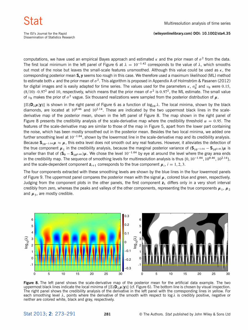
kE.D��jy/k is shown in the right panel of Figure 6 as a function of log10 �. The local minima, shown by the blackdiamonds, are located at 100.46 and 102.14. These are indicated by the two uppermost black lines in the scale-derivative map of the posterior mean, shown in the left panel of Figure 8. The map shown in the right panel ofFigure 8 presents the credibility analysis of the scale-derivative map where the credibility threshold ˛ D 0.95. Thefeatures of the scale-derivative map are similar to those of the map in Figure 5, apart from the lower part containingthe noise, which has been mostly smoothed out in the posterior mean. Besides the two local minima, we added onefurther smoothing level at 10�1.04, shown by the lowermost line in the scale-derivative map and its credibility analysis.Because S10�1.04� � �, this extra level does not smooth out any real features. However, it alleviates the detection ofthe true component �1 in the credibility analysis, because the marginal posterior variance of .S10�1.04 � S100.46/� issmaller than that of .S0 � S100.46/�. We chose the level 10�1.04 by eye at around the level where the gray area endsin the credibility map. The sequence of smoothing levels for multiresolution analysis is thus ¹0, 10�1.04, 100.46, 102.14º,and the scale-dependent component ziC1 corresponds to the true component �i, i D 1, 2, 3.

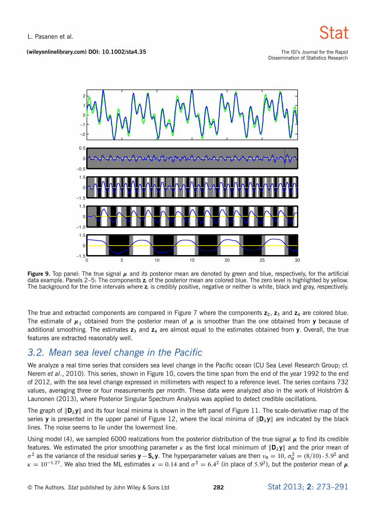
The four components extracted with these smoothing levels are shown by the blue lines in the four lowermost panelsof Figure 9. The uppermost panel compares the posterior mean with the signal �, colored blue and green, respectively.Judging from the component plots in the other panels, the first component z1 differs only in a very short intervalcredibly from zero, whereas the peaks and valleys of the other components, representing the true components �1, �2and �3, are mostly credible.

log 10

(λ)

0 5 10 15 20 25 30 0 5 10 15 20 25 30

−1

0

1

2

3

4

5

6

log 10

(λ)

−1

0

1

2

3

4

5

6

−0.3

−0.2

−0.1

0

0.1

0.2

0.3

Figure 8. The left panel shows the scale-derivative map of the posterior mean for the artificial data example. The twouppermost black lines indicate the local minima of kE.D��jy/k (cf. Figure 6). The bottom line is chosen by visual inspection.The right panel shows the credibility analysis of the derivative in the left panel with the corresponding lines in yellow. Foreach smoothing level �, points where the derivative of the smooth with respect to log� is credibly positive, negative orneither are colored white, black and gray, respectively.




−2

−1

0

1

2

−0.5

0

0.5

−1.5

0

1.5

−1.5

0

1.5

0 5 10 15 20 25 30−1.5

0

1.5

Figure 9. Top panel: The true signal � and its posterior mean are denoted by green and blue, respectively, for the artificialdata example. Panels 2–5: The components zi of the posterior mean are colored blue. The zero level is highlighted by yellow.The background for the time intervals where zi is credibly positive, negative or neither is white, black and gray, respectively.

The true and extracted components are compared in Figure 7 where the components z2, z3 and z4 are colored blue.The estimate of �1 obtained from the posterior mean of � is smoother than the one obtained from y because ofadditional smoothing. The estimates z3 and z4 are almost equal to the estimates obtained from y. Overall, the truefeatures are extracted reasonably well.

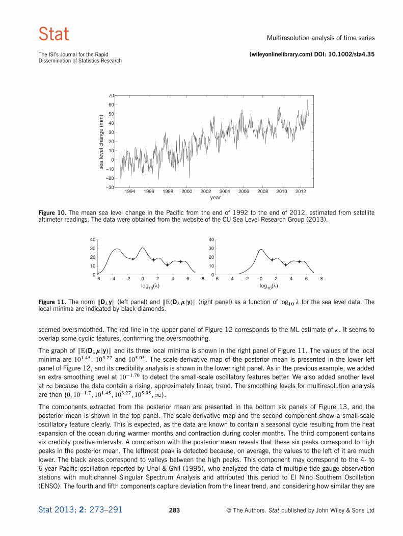
3.2. Mean sea level change in the PacificWe analyze a real time series that considers sea level change in the Pacific ocean (CU Sea Level Research Group; cf.Nerem et al., 2010). This series, shown in Figure 10, covers the time span from the end of the year 1992 to the endof 2012, with the sea level change expressed in millimeters with respect to a reference level. The series contains 732values, averaging three or four measurements per month. These data were analyzed also in the work of Holström &Launonen (2013), where Posterior Singular Spectrum Analysis was applied to detect credible oscillations.

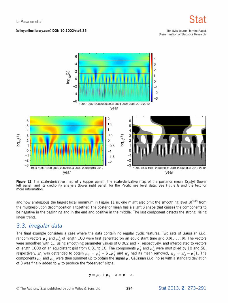
The graph of kD�yk and its four local minima is shown in the left panel of Figure 11. The scale-derivative map of theseries y is presented in the upper panel of Figure 12, where the local minima of kD�yk are indicated by the blacklines. The noise seems to lie under the lowermost line.

Using model (4), we sampled 6000 realizations from the posterior distribution of the true signal � to find its crediblefeatures. We estimated the prior smoothing parameter � as the first local minimum of kD�yk and the prior mean of�2 as the variance of the residual series y� S�y. The hyperparameter values are then �0 D 10, �20 D .8=10/ � 5.9

2 and� D 10�1.27. We also tried the ML estimates � D 0.14 and �2 D 6.42 (in place of 5.92), but the posterior mean of �




1994 1996 1998 2000 2002 2004 2006 2008 2010−30

−20

−10

0

10

20

30

40

50

60

Figure 10. The mean sea level change in the Pacific from the end of 1992 to the end of 2012, estimated from satellitealtimeter readings. The data were obtained from the website of the CU Sea Level Research Group (2013).

−6 −4 −2 0 2 4 6 80

−6 −4 −2 0 2 4 60

10

20

30

Figure 11. The norm kD�yk (left panel) and kE.D��jy/k (right panel) as a function of log10 � for the sea level data. Thelocal minima are indicated by black diamonds.

seemed oversmoothed. The red line in the upper panel of Figure 12 corresponds to the ML estimate of �. It seems tooverlap some cyclic features, confirming the oversmoothing.

The graph of kE.D��jy/k and its three local minima is shown in the right panel of Figure 11. The values of the localminima are 101.45, 103.27 and 105.05. The scale-derivative map of the posterior mean is presented in the lower leftpanel of Figure 12, and its credibility analysis is shown in the lower right panel. As in the previous example, we addedan extra smoothing level at 10�1.70 to detect the small-scale oscillatory features better. We also added another levelat 1 because the data contain a rising, approximately linear, trend. The smoothing levels for multiresolution analysisare then ¹0, 10�1.7, 101.45, 103.27, 105.05,1º.

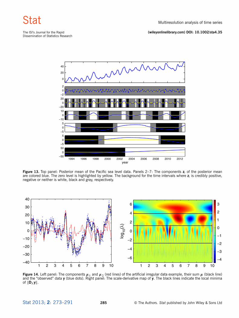
The components extracted from the posterior mean are presented in the bottom six panels of Figure 13, and theposterior mean is shown in the top panel. The scale-derivative map and the second component show a small-scaleoscillatory feature clearly. This is expected, as the data are known to contain a seasonal cycle resulting from the heatexpansion of the ocean during warmer months and contraction during cooler months. The third component containssix credibly positive intervals. A comparison with the posterior mean reveals that these six peaks correspond to highpeaks in the posterior mean. The leftmost peak is detected because, on average, the values to the left of it are muchlower. The black areas correspond to valleys between the high peaks. This component may correspond to the 4- to6-year Pacific oscillation reported by Unal & Ghil (1995), who analyzed the data of multiple tide-gauge observationstations with multichannel Singular Spectrum Analysis and attributed this period to El Niño Southern Oscillation(ENSO). The fourth and fifth components capture deviation from the linear trend, and considering how similar they are




Figure 12. The scale-derivative map of y (upper panel), the scale-derivative map of the posterior mean E.�jy/ (lowerleft panel) and its credibility analysis (lower right panel) for the Pacific sea level data. See Figure 8 and the text formore information.

and how ambiguous the largest local minimum in Figure 11 is, one might also omit the smoothing level 105.05 fromthe multiresolution decomposition altogether. The posterior mean has a slight S shape that causes the components tobe negative in the beginning and in the end and positive in the middle. The last component detects the strong, risinglinear trend.

3.3. Irregular dataThe final example considers a case where the data contain no regular cyclic features. Two sets of Gaussian i.i.d.random vectors �01 and �02 of length 100 were first generated on an equidistant time grid 0.01, : : : , 10. The vectorswere smoothed with (1) using smoothing parameter values of 0.002 and 7, respectively, and interpolated to vectorsof length 1000 on an equidistant grid from 0.01 to 10. The components �01 and �02 were multiplied by 10 and 50,respectively, �01 was detrended to obtain �1 D �01 � S1�01 and �02 had its mean removed, �2 D �02 � N�

021. The

components �1 and �2 were then summed up to obtain the signal �. Gaussian i.i.d. noise with a standard deviationof 3 was finally added to � to produce the “observed” signal

y D �1 C �2 C " D �C ".




0

20

40

−2

0

2

0

20

0

10

−5

0

5

−5

0

5

1994 1996 1998 2000 2002 2004 2006 2008 2010 2012

0

50

Figure 13. Top panel: Posterior mean of the Pacific sea level data. Panels 2–7: The components zi of the posterior meanare colored blue. The zero level is highlighted by yellow. The background for the time intervals where zi is credibly positive,negative or neither is white, black and gray, respectively.

0

10

20

30

log 10

(λ)

−6

−4

−2

0

2

4

6

0

1

2

3

Figure 14. Left panel: The components �1 and �2 (red lines) of the artificial irregular data example, their sum � (black line)and the “observed” data y (blue dots). Right panel: The scale-derivative map of y. The black lines indicate the local minimaof kD�yk.




The components �1 and �2, their sum � and the noisy series y are shown in the left panel of Figure 14. The scale-

derivative map of y is displayed in the right panel. The local minima of kD�yk are again indicated by the black lines.The lowermost segment of the scale-derivative map seems to capture the noise, and the second segment seems tocapture the small-scale feature �1. The large-scale component �2 is divided further into two components where thesmaller-scale component captures the features that are present in the right part of �2 and the larger-scale componentcaptures its overall U shape.

0

10

20

−2

0

2

0

20

0

20

0

20

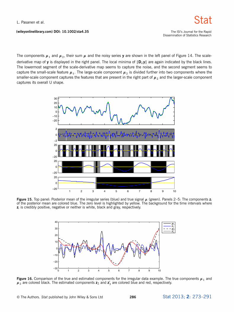
Figure 15. Top panel: Posterior mean of the irregular series (blue) and true signal � (green). Panels 2–5: The components ziof the posterior mean are colored blue. The zero level is highlighted by yellow. The background for the time intervals wherezi is credibly positive, negative or neither is white, black and gray, respectively.

Figure 16. Comparison of the true and estimated components for the irregular data example. The true components �1 and�2 are colored black. The estimated components z2 and z0

3are colored blue and red, respectively.




We then used model (4) for credibility analysis with a sample size of 6000. As �, we used 10�2.66, the smallestlocal minimum of kD�yk. The prior mean of �2 was estimated as the variance of the residual series y � S�y. Thevalues of the hyperparameters �, �20 and �0 are then 10�2.66, .8=10/ � 2.672 and 10, respectively. The values of �for multiresolution analysis were obtained from the local minima of kE.D��jy/k with a small value 10�2.11 addedto detect the small-scale features better, producing the sequence ¹0, 10�2.11, 101.21, 103.92º. The four extractedcomponents are presented in Figure 15. The second component seems to capture �1, and �2, having a variable scalealong the time axis, is represented by the sum of the third and fourth components. We therefore take z03 � z3C z4 andcompare z2 with �1 and z03 with �2. This comparison is shown in Figure 16. The original signal components �1 and�2 are reasonably well extracted, although the component z03 is somewhat rougher than the original component �2.

We also tried ML estimates for � and the prior mean of �2. The posterior mean was then smoother, but the extractedcomponents were very similar. The choice of � and the prior mean of �2 does not seem very crucial for the extractionof the components.

3.4. False-positivesWe compared the sensitivity of our method to false-positives with that of BSiZer by analyzing data that consist ofstandard Gaussian random vectors of length 100. The test was repeated 100 times, sampling 4000 vectors for eachrepetition from model (4) with �0 D 10 and �20 D .8=10/�

2ML and � D �ML, where �ML and �2ML are ML estimates. As a

result, 74 of the credibility maps of the derivative were completely gray, and 59 of the BSiZer maps were completelygray. The means of the estimated values of �ML and �2ML were 1.05 � 104 and 0.982, respectively. The maps with falsealarms typically had nongray areas only for large values of � but were otherwise blank.

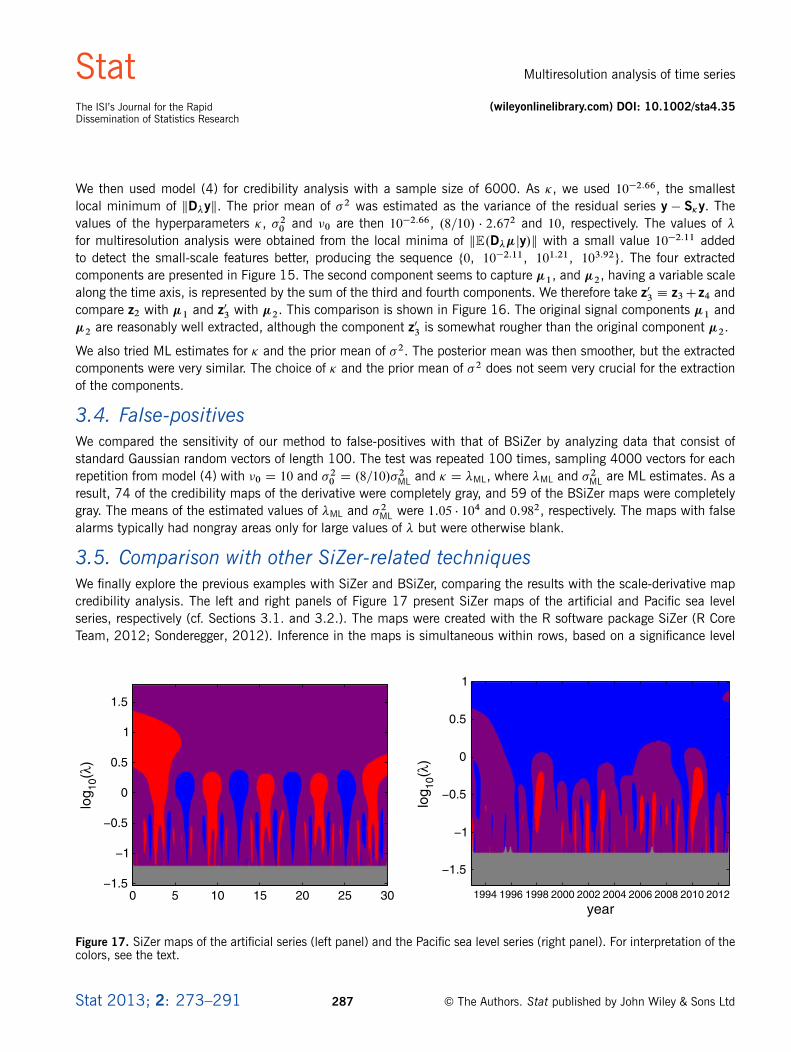
3.5. Comparison with other SiZer-related techniquesWe finally explore the previous examples with SiZer and BSiZer, comparing the results with the scale-derivative mapcredibility analysis. The left and right panels of Figure 17 present SiZer maps of the artificial and Pacific sea levelseries, respectively (cf. Sections 3.1. and 3.2.). The maps were created with the R software package SiZer (R CoreTeam, 2012; Sonderegger, 2012). Inference in the maps is simultaneous within rows, based on a significance level

Figure 17. SiZer maps of the artificial series (left panel) and the Pacific sea level series (right panel). For interpretation of thecolors, see the text.




of 0.95, and they are constructed using the extreme value theory as presented by Hannig & Marron (2006). TheSiZer maps are interpreted as follows. The pixels where the derivative with respect to time is significantly positive ornegative are colored blue and red, respectively. The remaining pixels are colored purple, except for those colored graywhere the data are too sparse for meaningful statistical inference.

In the left panel of Figure 17, the artificial series component �3 is clearly found around � D 100. The component �2 isdetected at around � D 10�0.5. However, the component �1 does not seem to be detected. Overall, the separation ofthe original components is clearer in the scale-derivative map (Figure 8, right panel). In the right panel, SiZer does not

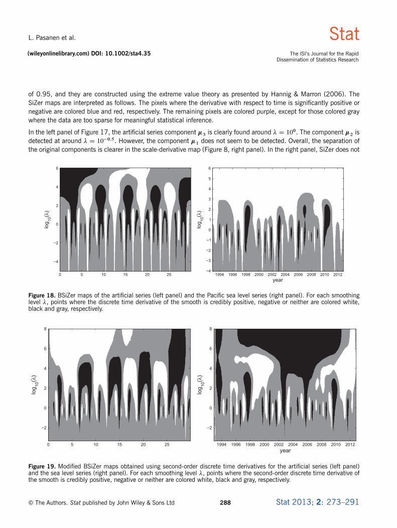
Figure 18. BSiZer maps of the artificial series (left panel) and the Pacific sea level series (right panel). For each smoothinglevel �, points where the discrete time derivative of the smooth is credibly positive, negative or neither are colored white,black and gray, respectively.

Figure 19. Modified BSiZer maps obtained using second-order discrete time derivatives for the artificial series (left panel)and the sea level series (right panel). For each smoothing level �, points where the second-order discrete time derivative ofthe smooth is credibly positive, negative or neither are colored white, black and gray, respectively.




seem to detect all the small-scale features. At higher scales, the high peaks and the S shape are also hard to detect.The separation of the cyclic components is also clearer in the scale-derivative map (Figure 12, lower right panel).BSiZer (Erästö & Holmström, 2005) was tried with the same posterior model and credibility used in Sections 3.1.and 3.2.. The resulting maps shown in Figure 18 are similar to the SiZer maps, except that a few more small-scalefeatures are detected.

We argued in Section 2.2. that the first derivative of a smooth with respect to � is approximately proportional to itssecond derivative with respect to time. We therefore also made comparisons with a modified BSiZer, where the first-order discrete time derivative is replaced with the second-order derivative. We used the same posterior model as beforeand drew the maps for the artificial and sea level series with the HPW method using a credibility threshold of 0.95.The results, presented in Figure 19, are rather similar to the scale-derivative map credibility analyses of Figures 8and 12. However, in the left panel of Figure 19, the small-scale feature �1 of the artificial series is not completelydetected. In the right panel, the small-scale features of the sea level series do seem to be detected as well as in thescale-derivative map. The modified BSiZer maps and the credibility analyses of the scale-derivative maps differ in theupper parts where the smoothing level is large with respect to the length of the series, as boundary conditions startto influence the results. We also drew SiZer maps based on the second derivatives. They were relatively similar to themodified BSiZer maps, although fewer small-scale features were detected.

4 DiscussionWe proposed a method for extracting time series features in different scales. The method constructs a scale-derivativemap of the smooths of the series together with its credibility analysis. The maps help detect features of the data indifferent scales in the same spirit as SiZer-related methods. However, whereas SiZer considers time derivatives, wedifferentiate along the logarithmic scale axis. As a result, instead of finding where the series increases or decreases, wedetect time points where the series is larger or smaller than its average in a local neighborhood. The local minima ofthe norm of the scale derivative are then selected as the sequence of smoothing levels that extract the scale-dependentcomponents of the time series, producing a multiresolution analysis.

The scale-derivative map and the scale-dependent components can be computed directly from noisy observations,which can already provide valuable information about the data. However, to separate true features from artifacts ofnoise, Bayesian inference is used. We assumed an i.i.d. Gaussian noise, but the method is easily extended to differentnoise models or even to a case where the time grid is random (Erästö & Holmström, 2007), as the posterior model isindependent of the rest of the method.

If the smooths were differentiated with respect to � instead of log�, the magnitude of the derivative would diminish,with larger scales making the upper parts of the maps nearly featureless. For the same reason, the maps of thesecond time derivatives would not be as meaningful if viewed directly. Hence, although the scale-derivative mapcredibility analyses and the modified BSiZer maps look similar, the advantage of differentiating with respect to log�is that, instead of just indicating credibly positive or negative derivatives, the magnitude and sign of the derivative ismore clearly displayed. For the same reason, the scale-dependent components cannot be extracted using the modifiedBSiZer.

Spline smoothing was employed, but the method could use other smoothers, too. The fact that the heat equationrelates to Gaussian convolution motivated us to try local linear regression used in SiZer, as it resembles Gaussianconvolution more than spline smoothing. We approximated the scale-derivative map with the difference quotient




�.S� � S��/�=log � , whereas posterior sampling and credibility analysis were performed as before. The high-frequency sine of the artificial series was not detected completely. The results of the irregular series example werequite similar for local linear regression and smoothing splines, whereas in the sea level example, a few more small-scale spikes were detected with local linear regression. In the work of Marron & Zhang (2005), spline and local linearregression SiZers were compared, and according to the authors, the “smoothing spline method is effective in smooth-ing low noise but sparse data, while the local linear method performs better for high noise but dense data,” which isin line with our findings.

We demonstrated our method with two artificial examples and one real time series involving sea level change inthe Pacific. The scale-derivative map separated the oscillatory features, and the scale-dependent components thusextracted were mostly credible. The last example was composed of an irregular artificial series that did not containclear oscillatory features, but the proposed method seemed to perform well. The estimates of the prior smoothingparameter chosen as the first local minimum of kD�yk had smaller values than those calculated with the ML method.In the case of the artificial examples, ML seemed to produce posterior means that were closer to the true signal.For the sea level series, however, the prior smoothing parameter estimate from the scale-derivative map appeared toperform better than the ML estimate, which caused oversmoothing. Therefore, the scale-derivative map may also offera means to evaluate the quality of the prior smoothing parameter estimate.

We compared the results of the first artificial example and the sea level example with SiZer maps and observed thatespecially the oscillatory features were more clearly separated in our scale-derivative maps. The scale-derivative mapsof the examples seemed to detect features more sensitively than BSiZer, and the scale-derivative map may also be lessprone to false-positives. The modified BSiZer based on second derivatives produced results that were rather similar tothe scale-derivative maps. However, the credibility analysis of the scale-derivative maps seemed to color more areascredible, especially for the artificial series.

AcknowledgmentThis study was funded by the Academy of Finland under grant no. 250862.

ReferencesChaudhuri, P & Marron, JS (1999), ‘SiZer for exploration of structures in curves’, Journal of the American Statistical

Association, 94(447), 807–823.

Chaudhuri, P & Marron, JS (2000), ‘Scale space view of curve estimation’, The Annals of Statistics, 28(2), 408–428.

CU Sea Level Research Group (2013), Global and regional mean sea level time series. Available online at http://sealevel.colorado.edu/. Accessed in February 2013.

Erästö, P & Holmström, L (2005), ‘Bayesian multiscale smoothing for making inferences about features in scatterplots’, Journal of Computational and Graphical Statistics, 14(3), 569–589.

Erästö, P & Holmström, L (2007), ‘Bayesian analysis of features in a scatter plot with dependent observations anderrors in predictors’, Journal of Statistical Computation and Simulation, 77(5), 421–431.

Godtliebsen, F & Øigård, T (2005), ‘A visual display device for significant features in complicated signals’,Computational Statistics & Data Analysis, 48(2), 317–343.


http://sealevel.colorado.edu/

http://sealevel.colorado.edu/



Hannig, J & Marron, JS (2006), ‘Advanced distribution theory for SiZer’, Journal of the American StatisticalAssociation, 101(474), 484–499.

Holmström, L (2010a), ‘BSiZer’, Wiley Interdisciplinary Reviews: Computational Statistics, 2 (5), 526–534.Available online at http://dx.doi.org/10.1002/wics.115.

Holmström, L (2010b), ‘Scale space methods’, Wiley Interdisciplinary Reviews: Computational Statistics, 2 (2),150–159. Available online at http://dx.doi.org/10.1002/wics.79.

Holmström, L & Launonen, I (2013), ‘Posterior singular spectrum analysis’, Statistical Analysis and Data Mining, 6,387–402, DOI 10.1002/sam.11195.

Holmström, L & Pasanen, L (2012), ‘Bayesian scale space analysis of differences in images’, Technometrics, 54(1),16 –29, DOI 10.1080/00401706.2012.648862.

Holmström, L, Pasanen, L, Furrer, R & Sain, SR (2011), ‘Scale space multiresolution analysis of random signals’,Computational Statistics & Data Analysis, 55(10), 2840 –2855. Available online at http://dx.doi.org/10.1016/j.csda.2011.04.011.

Lindeberg, T (1994), Scale-space Theory in Computer Vision, Kluwer Academic Publishers , Dordrecht, Netherlands.

Marr, D & Hildreth, E (1980), ‘Theory of edge detection’, Proceedings of the Royal Society of London. Series B,Biological Sciences, 207(1167), 187–217, DOI 10.2307/35407.

Marron, JS & Zhang, J (2005), ‘SiZer for smoothing splines’, Computational Statistics, 20, 481–502, DOI10.1007/BF02741310.

Nerem, RS, Chambers, D, Choe, C & Mitchum, GT (2010), ‘Estimating mean sea level change from the TOPEX andJason altimeter missions’, Marine Geodesy, 33, 435.

R Core Team (2012), R: A Language and Environment for Statistical Computing, R Foundation for StatisticalComputing, Vienna, Austria. ISBN 3-900051-07-0.

Sonderegger, D (2012), Sizer: Significant Zero Crossings. R package version 0.1-4.

Unal, YS & Ghil, M (1995), ‘Interannual and interdecadal oscillation patterns in sea level’, Climate Dynamics, 11,255–278.


http://dx.doi.org/10.1002/wics.115

http://dx.doi.org/10.1002/wics.79

http://dx.doi.org/10.1016/j.csda.2011.04.011

http://dx.doi.org/10.1016/j.csda.2011.04.011

A scale space multiresolution method for extraction of time series features

Documents

Transcript of A scale space multiresolution method for extraction of time series features