Journal of Computational and Applied Mathematics 119 (2000) 97–114www.elsevier.nl/locate/cam

Multiresolution analysis over triangles, based on quadraticHermite interpolation(

M. D�hlen, T. Lyche, K. M�rken ∗, R. Schneider, H-P. SeidelDepartment of Informatics, University of Oslo, P.O. Box 1080 Blindern, 0316 Oslo, Norway

Received 29 November 1999

Dedicated to Prof. Larry L. Schumaker on the occasion of his 60th birthday

Abstract

Given a triangulation T of R2, a recipe to build a spline space S(T ) over this triangulation, and a recipe to re�ne thetriangulation T into a triangulation T ′, the question arises whether S(T )⊂S(T ′), i.e., whether any spline surface overthe original triangulation T can also be represented as a spline surface over the re�ned triangulation T ′. In this paper wewill discuss how to construct such a nested sequence of spaces based on Powell–Sabin 6-splits for a regular triangulation.The resulting spline space consists of piecewise C1-quadratics, and re�nement is obtained by subdividing every triangleinto four subtriangles at the edge midpoints. We develop explicit formulas for wavelet transformations based on quadraticHermite interpolation, and give a stability result with respect to a natural norm. c© 2000 Elsevier Science B.V. All rightsreserved.

MSC: 41A63; 65D07; 65D17; 65T60

Keywords: Multivariate splines; Triangulations; Wavelets

1. Introduction

In [2] we developed a multiresolution setup for quadratic splines based on Hermite interpolation.This was based on the hierarchical basis of Faber [3], see also [9]. In this paper we generalize thisunivariate, quadratic construction to bivariate, piecewise quadratic functions de�ned on a given regu-lar triangulation. Multiresolution over triangles is well known, see, e.g., [5,6,9], and there are severalapproaches that extend to spheres [11] or even surfaces of arbitrary topology [8]. Unfortunately, most

( This work has been sponsored by NATO Collaborative Research Grant “E�cient Hierarchical Representation of Curvesand Surfaces”.

∗ Corresponding author.E-mail address: knutm@i�.uio.no (K. M�rken).

0377-0427/00/$ - see front matter c© 2000 Elsevier Science B.V. All rights reserved.PII: S 0377-0427(00)00373-3

98 M. D�hlen et al. / Journal of Computational and Applied Mathematics 119 (2000) 97–114

of the occurring bases result from subdivision algorithms and therefore cannot be represented explic-itly. The basis constructed in this paper overcomes that drawback and is also suited to be extendedto surfaces of arbitrary topology by adapting the rationale described in [8].The construction of a multiresolution analysis over a triangulation is closely connected with the

construction of nested polynomial spline spaces, see [7]. In that paper there is a distinction betweentwo major approaches: either the triangulation or the polynomial degree is kept �xed. Since we wantto extend the univariate method, we choose to keep the degree �xed, i.e., we re�ne the triangulationto get nested spline spaces

V0⊂V1⊂ · · ·⊂Vk ⊂ · · · :For piecewise quadratic polynomials that are C1, the dimension of the spline space is too low toallow a reasonable basis, so to use quadratic spines we will have to introduce macro patches. Wewill make use of the Powell–Sabin 6-split [10] which combines nicely with Hermite interpolation.

2. Multiresolution analysis

In this section we brie y summarize what is meant by a multiresolution analysis and a weaklystable basis. We need a fairly general de�nition of multiresolution analysis, see [1], and also [2] fora speci�c discussion relevant to the setting in this paper.

De�nition 1. A multiresolution analysis consists of1. A Banach space F of functions de�ned on a bounded set X ⊂Rn, with n¿ 0 and with associatednorm || · ||.

2. A nested sequence of subspaces V0⊂V1⊂ · · ·⊂Vk ⊂ · · · that are dense in F,

∞⋃k=1

Vk =F:

3. A collection of uniformly bounded operators

Qk :F → Vk

with the properties

QkQk = Qk;

QkQk+1 = Qk;

Qk(F) = Vk

for all integers k¿0.

With the projectors Qk given, we can de�ne the complement spaces

Wk = {F ∈ Vk+1 |QkF = 0}

M. D�hlen et al. / Journal of Computational and Applied Mathematics 119 (2000) 97–114 99

and using the fact that Vk+1 = Vk + Wk and Vk ∩ Wk = {0}, we get a decomposition of F as thedirect sum

F= V0 +W0 +W1 +W2 + · · · :This means that every F ∈ F can be decomposed as

F = F0 + G0 + G1 + G2 + · · ·with Gk = Fk+1 − Fk in Wk . For simplicity, we will refer to the complement spaces Wk as waveletspaces and functions in Wk as wavelets, although it is common to require from wavelets that theyhave a number of vanishing moments.Let {�j;k}j∈Ik (often referred to as scaling functions) be a basis for Vk indexed by the index set

Ik , and let { j; k}j∈Jk be a basis for Wk , with index set Jk . Since nearly all information of a functionF ∈ F is included in

⋃∞k=0Wk , it is crucial to know the stability properties of the wavelet functions,

which relate the size of a function to the size of its wavelet coe�cients. Let Fn=∑n

k=1

∑j∈Jk

dj; k j; kbe the representation of a wavelet function, then we will employ an, as yet unspeci�ed, vector norm

�n = ||(dj;k)nk=1; j∈Jk||v (1)

to measure the size of the wavelet coe�cients.We will be working with uniform norms, so a weaker form of stability than usual is convenient.

De�nition 2. Let F be a space with a multiresolution analysis and corresponding wavelet bases{ j; k}: The wavelets are said to form a weakly stable basis for

⋃∞k=1Wk if for each n¿1 there exist

constants K1; n and K2; n such that

K−11; n �n6

∣∣∣∣∣∣∣∣∣∣∣∣

n∑k=1

∑j∈Jk

dj; k j; k

∣∣∣∣∣∣∣∣∣∣∣∣6K2; n�n;

where �n is given by (1), and K1; n and K2; n have at most polynomial growth in n. If the two constantsK1; n and K2; n are independent of n, the basis is said to be strongly stable.

3. Multiresolution based on quadratic Hermite interpolation

In the following, we will derive a multiresolution analysis built over an equilateral triangle, butthis can be generalized to any regular triangulation. Consider a triangulation de�ned on the regularhexagon with centre point P0 at the origin and edge vertices Pl with P1 = (2; 0), with the othervertices chosen counterclockwise around the circle of radius 2,

Pl = 2

(cos(l− 1)�=3sin(l− 1)�=3

)for l= 1; : : : ; 6:

These seven points generate a triangulation consisting of six equilateral triangles. On every trianglewe perform a Powell–Sabin 6-split by connecting each vertex with the midpoint of its oppositeedge, so we get a new triangulation THEX. We denote by S12(THEX) all C1-functions that reduce toa quadratic polynomial on each triangle in THEX. It is well known that each function in S12(THEX)

100 M. D�hlen et al. / Journal of Computational and Applied Mathematics 119 (2000) 97–114

is uniquely determined by its position and �rst derivatives at the seven points {Pl}6l=0, (see [4]). Wecan therefore introduce three nodal functions C1, C2 and C3 that are characterized by the conditions

C1(Pl) = �l;0; C2(Pl) = 0; C3(Pl) = 0;

@@x

C1(Pl) = 0;@@x

C2(Pl) = �l;0;@@x

C3(Pl) = 0; (2)

@@y

C1(Pl) = 0;@@y

C2(Pl) = 0;@@y

C3(Pl) = �l;0

for l= 0; 1; : : : ; 6. The B�ezier representation of these functions is shown in Fig. 1.It is now straightforward to build a multiresolution analysis on an equilateral triangle D using

dilates and translates of C1; C2 and C3. We choose D to be the subtriangle of our hexagon withvertices P0; P1; P2, and introduce the domain points

�k =

�i; j; k = i

P1 − P02k

+ jP2 − P02k

=12k

2i + j

√3j

∣∣∣∣∣∣ i¿0; j¿0; i + j62k

:

For each domain point �i; j; k we de�ne the three scaling functions

�li; j; k(x; y) =

12k

Cl(2kx − 2i − j; 2ky −√3j) for l= 1; 2; 3;

where the factor 1=2k has been introduced to simplify the arithmetic and stability results followinglater. We get a sequence of nested spline spaces as the span of these functions

Vk = spani¿0; j¿0; i+j62k {�1i; j; k ; �

2i; j; k ; �

3i; j; k}

restricted to the triangle D.We can now constuct Hermite interpolation operators. We choose Qk :C1(D) → Vk , so that for

every F ∈ C1(D) the projection Fk = QkF has the properties

Fk(�i; j; k) = F(�i; j; k);

@@x

Fk(�i; j; k) =@@x

F(�i; j; k);

@@y

Fk(�i; j; k) =@@y

F(�i; j; k)

for all points �i; j; k ∈ �k . From the inclusion �k ⊂�k+1 and uniqueness of interpolation, it followsthat Qk satis�es QkQk =Qk and QkQk+1 =Qk . By de�nition, the wavelet space Wk consists of thosefunctions in Vk+1 whose position and �rst derivatives vanish at the points of �k ,

Wk ={Fk+1 ∈ Vk+1 |Fk+1(�i; j; k) = 0;

@@x

Fk+1(�i; j; k) = 0;@@y

Fk+1(�i; j; k) = 0; ∀�i; j; k ∈ �k

}:

M. D�hlen et al. / Journal of Computational and Applied Mathematics 119 (2000) 97–114 101

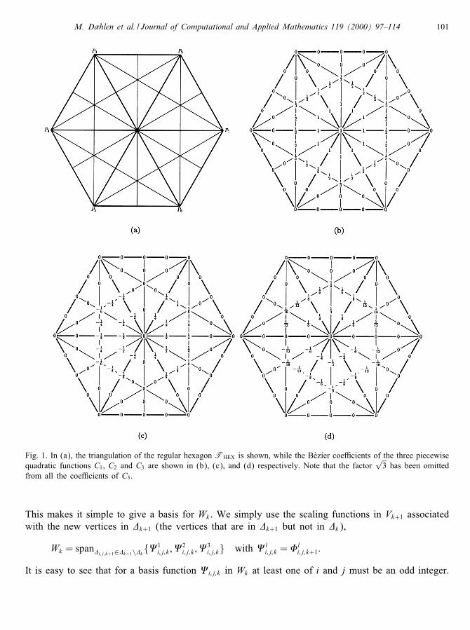
Fig. 1. In (a), the triangulation of the regular hexagon THEX is shown, while the B�ezier coe�cients of the three piecewisequadratic functions C1, C2 and C3 are shown in (b), (c), and (d) respectively. Note that the factor

√3 has been omitted

from all the coe�cients of C3.

This makes it simple to give a basis for Wk . We simply use the scaling functions in Vk+1 associatedwith the new vertices in �k+1 (the vertices that are in �k+1 but not in �k),

Wk = span�i; j; k+1∈�k+1\�k{1

i; j; k ; 2i; j; k ;

3i; j; k} with l

i; j; k = �li; j; k+1:

It is easy to see that for a basis function i;j; k in Wk at least one of i and j must be an odd integer.

102 M. D�hlen et al. / Journal of Computational and Applied Mathematics 119 (2000) 97–114

We now have the basic ingredients for building a multiresolution analysis. As our space F wetake C1(D), the space of functions de�ned on the triangle D that are continuous and have continuous�rst derivatives in D, and the norm we take to be

||F ||=max{||F ||L∞(D);

∣∣∣∣∣∣∣∣@F@x

∣∣∣∣∣∣∣∣L∞(D)

;∣∣∣∣∣∣∣∣@F@y

∣∣∣∣∣∣∣∣L∞(D)

}; (3)

where ||F ||∞ denotes the usual L∞-norm for functions de�ned on D.Because of (2), it is easy to determine the coe�cients of a spline Fk =

∑�i; j; k∈�k

ali; j; k�

li; j; k in Vk ,

a1i; j; k = 2kF(�i; j; k);

a2i; j; k =@@x

F(�i; j; k);

a3i; j; k =@@y

F(�i; j; k); (4)

where∑

�i; j; k∈�kdenotes the sum of all index pairs (i; j) with �i; j; k ∈ �k . These simple formulas will

be useful later.To verify that we have a multiresolution analysis it remains to check that the operators {Qk} are

uniformly bounded and that the spaces {Vk} are dense in C1(D). This is tedious but straightforward,and is postponed until Section 6.

4. Reconstruction and decomposition algorithms

The fundamental algorithms for dealing with wavelets are the wavelet transform and inversewavelet transform, or the decomposition algorithm and the reconstruction algorithm. The decompo-sition algorithm starts with a spline Fk+1 in Vk+1 and decomposes this into Fk+1=Fk+Gk with Fk inVk and Gk in Wk . This process can be iterated to produce the decomposition Fk+1=F0+G0+· · ·+Gk ,but it su�ces to show how the �rst step is to be performed. The reconstruction algorithm undoesthe decomposition and produces Fk+1 from the two components Fk and Gk . We start by describingthe reconstruction algorithm.

4.1. The reconstruction algorithm

Since Vk ⊆Vk+1, the scaling functions in Vk can be written as linear combinations of the scalingfunctions in Vk+1. From (4) it follows that the coe�cients are given by function values and �rstderivatives of the scaling functions in Vk at the knots �k+1. Since �l

i; j; k(x; y)= (1=2k)Cl(2kx− 2i− j;

2ky −√3j), this means we have to calculate the values of Cl, (@=@x)Cl and (@=@y)Cl at the knots

�i; j;1, and these values can be easily derived from the B�ezier representations of {Cl}3l=1. The resultis some long formulas which we omit here, but with that information we can lift a function Fk in

M. D�hlen et al. / Journal of Computational and Applied Mathematics 119 (2000) 97–114 103

Vk into Vk+1. More speci�cally, if

Fk =∑(i; j)∈Ikl=1;2;3

ali; j; k�

li; j; k

∣∣∣∣∣D

=∑

(i; j)∈Ik+1l=1;2;3

ali; j; k+1�

li; j; k+1

∣∣∣∣∣D

; (5)

we obtain formulas for all the re�ned coe�cients (ali; j; k+1) in terms of the coarser coe�cients (a

li; j; k).

But this is not the complete reconstruction algorithm. In general, we also have a wavelet componentGk so that Fk+1 = Fk + Gk . But since

Gk =∑

�i; j; k+1∈�k+1\�k

l=1;2;3

bli; j; k

li; j; k with l

i; j; k = �li; j; k+1;

we obtain the coe�cients (ali; j; k+1) by adding bl

i; j; k to the coe�cient ali; j; k+1 for every �i; j; k+1 with at

least one odd i or j, i.e.,

a12i;2j; k+1 = 2a1i; j; k ;

a22i;2j; k+1 = a2i; j; k ;

a32i;2j; k+1 = a3i; j; k ;

a12i+1;2j; k+1 = b12i+1;2j; k+1 + (a1i; j; k + a1i+1; j; k) +

12(a

2i; j; k − a2i+1; j; k);

a22i+1;2j; k+1 = b22i+1;2j; k+1 + (−a1i; j; k + a1i+1; j; k)− 12 (a

2i; j; k + a2i+1; j; k);

a32i+1;2j; k+1 = b32i+1;2j; k+1 +12(a

3i; j; k + a3i+1; j; k);

a12i;2j+1; k+1 = b12i;2j+1; k+1 + (a1i; j; k + a1i; j+1; k) +

14(a

2i; j; k − a2i; j+1; k) +

14

√3(a3i; j; k − a3i; j+1; k);

a22i;2j+1; k+1 = b22i;2j+1; k+1 +12(−a1i; j; k + a1i; j+1; k) +

14(a

2i; j; k + a2i; j+1; k)− 1

4

√3(a3i; j; k + a3i; j+1; k);

a32i;2j+1; k+1 = b32i;2j+1; k+1 +12

√3(−a1i; j; k + a1i; j+1; k)− 1

4

√3(a2i; j; k + a2i; j+1; k)− 1

4 (a3i; j; k + a3i; j+1; k);

a12i+1;2j+1; k+1 = b12i+1;2j+1; k+1 + (a1i; j+1; k + a1i+1; j; k) +

14(a

2i; j+1; k − a2i+1; j; k) +

14

√3(−a3i; j+1; k + a3i+1; j; k);

a22i+1;2j+1; k+1 = b22i+1;2j+1; k+1+12(−a1i; j+1; k+a1i+1; j; k)+

14(a

2i; j+1; k+a2i+1; j; k)+

14

√3(a3i; j+1; k+a3i+1; j; k);

a32i+1;2j+1; k+1 = b32i+1;2j+1; k+1+12

√3(a1i; j+1; k − a1i+1; j; k)+

14

√3(a2i; j+1; k+a2i+1; j; k)− 1

4 (a3i; j+1; k+a3i+1; j; k):

(6)

If we look more carefully at these formulas we note that they can be written in block matrix–vectorform as(

aevenk+1

aoddk+1

)=

(D 0

M I

)(ak

bk

): (7)

104 M. D�hlen et al. / Journal of Computational and Applied Mathematics 119 (2000) 97–114

Here aevenk+1 is the vector of coe�cients on level k + 1 for which both indices are even, while theremaining coe�cients on level k + 1 are grouped together in aoddk+1. Similarly, the coe�cients of Fk

are grouped together in ak and the coe�cients of Gk in bk . The matrix D is a diagonal matrix with1s and 2s on the diagonal corresponding to the �rst three equations in (6), while the matrix M isthe matrix that guides how the coe�cients in ak are combined in the remaining formulas in (6).

4.2. The decomposition algorithm

The decomposition formula is easily obtained by inverting the reconstruction formulas. From (7)we see that ak and bk can be expressed in terms of the coe�cients on level k + 1 by inverting thatrelation(

ak

bk

)=

(D−1 0

−MD−1 I

)(aevenk+1

aoddk+1

):

For the coe�cients of Fk we then �nd

a1i; j; k =12a12i;2j; k+1;

a2i; j; k = a22i;2j; k+1;

a3i; j; k = a32i;2j; k+1;

while the wavelet coe�cients are given by

b12i+1;2j; k = al2i+1;2j; k+1 − 1

2 (a12i;2j; k+1 + a12i+2;2j; k+1)− 1

2 (a22i;2j; k+1 − a22i+2;2j; k+1);

b22i+1;2j; k = a22i+1;2j; k+1 − 12 (−a12i;2j; k+1 + a12i+2;2j; k+1)− 1

2 (a22i;2j; k+1 + a22i+2;2j; k+1);

b32i+1;2j; k = a32i+1;2j; k+1 − 12 (a

32i;2j; k+1 + a32i+2;2j; k+1);

b12i;2j+1; k = a12i;2j+1; k+1 − 12 (a

12i;2j; k+1 + a12i;2j+2; k+1)

− 14 (a

22i;2j; k+1 − a22i;2j+2; k+1)− 1

4

√3(a32i;2j; k+1 − a32i;2j+2; k+1);

b22i;2j+1; k = a22i;2j+1; k+1 − 14 (−a12i;2j; k+1 + a12i;2j+2; k+1)

− 14 (a

22i;2j; k+1 + a22i;2j+2; k+1) +

14

√3(a32i;2j; k+1 + a32i;2j+2; k+1);

b32i;2j+1; k = a32i;2j+1; k+1 − 14

√3(−a12i;2j; k+1 + a12i;2j+2; k+1)

+14

√3(a22i;2j; k+1 + a22i;2j+2; k+1) +

14(a

32i;2j; k+1 + a32i;2j+2; k+1);

b12i+1;2j+1; k = a12i+1;2j+1; k+1 − 12 (a

12i;2j+2; k+1 + a12i+2;2j; k+1)

− 14 (a

22i;2j+2; k+1 − a22i+2;2j; k+1)− 1

4

√3(−a32i;2j+2; k+1 + a32i+2;2j; k+1);

M. D�hlen et al. / Journal of Computational and Applied Mathematics 119 (2000) 97–114 105

b22i+1;2j+1; k = a22i+1;2j+1; k+1 − 14 (−a12i;2j+2; k+1 + a12i+2;2j; k+1)

− 14 (a

22i;2j+2; k+1 + a22i+2;2j; k+1)− 1

4

√3(a32i;2j+2; k+1 + a32i+2;2j; k+1);

b32i+1;2j+1; k = a32i+1;2j+1; k+1 − 14

√3(a12i;2j+2; k+1 − a12i+2;2j; k+1)

− 14

√3(a22i;2j+2; k+1 + a22i+2;2j; k+1) +

14(a

32i;2j+2; k+1 + a32i+2;2j; k+1): (8)

Note that only the coe�cients associated with �i; j; k+1 and its two neighbors in �k have an in uenceon bl

i; j; k . This means that decomposition and reconstruction along an edge of the triangle D can bedone if we know the corresponding values along that edge. This fact guarantees that there is noneed for a special treatment at the boundary of the parameter domain.We also observe that we get the same formulas for a1i; j; k , a

2i; j; k , b

12i+1;2j; k and b22i+1;2j; k as for the

corresponding coe�cients in the univariate case, taking into account that we introduced the factor1=2k in the de�nition of our scaling functions (cf. [2]).

5. Stability

In this section we want to prove that the wavelet basis is weakly stable. Most of the work is donein the next lemma.

Lemma 3. Let Gk be the wavelet component of F in Wk given by

Gk = Qk+1F − QkF =∑

�i; j; k+1∈�k+1\�k

l=1;2;3

bli; j; k

li; j; k ;

where F is assumed to lie in C1(D). Then the wavelet coe�cients are bounded by

|b12i+1;2j; k |63∣∣∣∣∣∣∣∣ @@xF

∣∣∣∣∣∣∣∣L∞(J 1)

;

|b22i+1;2j; k |64∣∣∣∣∣∣∣∣ @@xF

∣∣∣∣∣∣∣∣L∞(J 1)

;

|b32i+1;2j; k |62∣∣∣∣∣∣∣∣ @@yF

∣∣∣∣∣∣∣∣L∞(J 1)

;

|b12i;2j+1; k |632(1 +

√3)max

{∣∣∣∣∣∣∣∣ @@xF

∣∣∣∣∣∣∣∣L∞(J 2)

;∣∣∣∣∣∣∣∣ @@yF

∣∣∣∣∣∣∣∣L∞(J 2)

};

|b22i;2j+1; k |6(2 +√3)max

{∣∣∣∣∣∣∣∣ @@xF

∣∣∣∣∣∣∣∣L∞(J 2)

;∣∣∣∣∣∣∣∣ @@yF

∣∣∣∣∣∣∣∣L∞(J 2)

};

106 M. D�hlen et al. / Journal of Computational and Applied Mathematics 119 (2000) 97–114

|b32i;2j+1; k |6(3 +√3)max

{∣∣∣∣∣∣∣∣ @@xF

∣∣∣∣∣∣∣∣L∞(J 2)

;∣∣∣∣∣∣∣∣ @@yF

∣∣∣∣∣∣∣∣L∞(J 2)

};

|b12i+1;2j+1; k |632(1 +

√3)max

{∣∣∣∣∣∣∣∣ @@xF

∣∣∣∣∣∣∣∣L∞(J 3)

;∣∣∣∣∣∣∣∣ @@yF

∣∣∣∣∣∣∣∣L∞(J 3)

};

|b22i+1;2j+1; k |6(2 +√3)max

{∣∣∣∣∣∣∣∣ @@xF

∣∣∣∣∣∣∣∣L∞(J 3)

;∣∣∣∣∣∣∣∣ @@yF

∣∣∣∣∣∣∣∣L∞(J 3)

};

|b32i+1;2j+1; k |6(3 +√3)max

{∣∣∣∣∣∣∣∣ @@xF

∣∣∣∣∣∣∣∣L∞(J 3)

;∣∣∣∣∣∣∣∣ @@yF

∣∣∣∣∣∣∣∣L∞(J 3)

}:

In any subtriangle T with vertices �i; j; k ; �i+1; j; k ; �i; j+1; k or �i; j; k ; �i+1; j; k ; �i+1; j−1; k the estimates

||Gk ||L∞(T )612k+1

(32+

√36

)max(i; j)∈Il=1;2;3

{|bli; j; k |};

∣∣∣∣∣∣∣∣ @@xGk

∣∣∣∣∣∣∣∣L∞(T )

6

(3 +

√33

)max(i; j)∈Il=1;2;3

{|bli; j; k |};

∣∣∣∣∣∣∣∣ @@yGk

∣∣∣∣∣∣∣∣L∞(T )

6(1 +

53

√3)max(i; j)∈Il=1;2;3

{|bli; j; k |} (9)

hold. Here J 1 is the line between �2i;2j; k+1 and �2i+2;2j; k+1; while J 2 is the line between �2i;2j; k+1and �2i;2j+2; k+1 and J 3 is the line between �2i;2j+2; k+1 and �2i+2;2j; k+1. The index set I consists ofthe midpoints of the edges of T .

Proof. Note that this proof makes use of Lemma 5 and its proof.The inequalities for the coe�cients are immediate consequences of the decomposition relations.

Since the proof is nearly the same in all nine cases, we only verify the inequality for b12i;2j+1; k . From(8) and (4) we have

b12i;2j+1; k =12(a12i;2j+1; k+1 − a12i;2j; k+1)−

12(a12i;2j+2; k+1 − a12i;2j+1; k+1)

− 14(a22i;2j; k+1 − a22i;2j+2; k+1)−

14

√3(a32i;2j; k+1 − a32i;2j+2; k+1)

= 2k(F(�2i;2j+1; k+1)− F(�2i;2j; k+1))− 2k(F(�2i;2j+2; k+1)− F(�2i;2j+1; k+1))

− 14

(@@x

F(�2i;2j; k+1)− @@x

F(�2i;2j+2; k+1))

− 14

√3(

@@y

F(�2i;2j; k+1)− @@y

F(�2i;2j+2; k+1)): (10)

M. D�hlen et al. / Journal of Computational and Applied Mathematics 119 (2000) 97–114 107

Applying the mean-value theorem we �nd

2k(F(�2i;2j+1; k+1)− F(�2i;2j; k+1)

)= 〈∇F(�1); C〉= 1

2@@x

F(�1) +12

√3

@@y

F(�1);

2k(F(�2i;2j+2; k+1)− F(�2i;2j+1; k+1)) = 〈∇F(�2); C〉= 12

@@x

F(�2) +12

√3

@@y

F(�2);

where �1 and �2 lie in J 2 and Ct =(12 ;12

√3). Inserting these two expressions in (10) we obtain the

required result.The inequalities (9) for ||Gk ||L∞(T ), ||(@=@x)Gk ||L∞(T ) and ||(@=@y)Gk ||L∞(T ) can be obtained from

(22), since Gk |T can be expressed in terms of only nine nonzero basis functionsGk |T =

∑(i′ ; j′)∈Il=1;2;3

(bli′ ; j′ ; k

li′ ; j′ ; k |T ):

Here I denotes the midpoint index set for the triangle T , i.e., if T has vertices �2i;2j; k+1, �2i+2;2j; k+1,�2i;2j+2; k+1 we have I = {(2i + 1; 2j); (2i; 2j + 1); (2i + 1; 2j + 1)} whereas if the vertices of T are�2i;2j; k+1, �2i+2;2j; k+1, �2i+2;2j−2; k+1 we have I = {(2i + 1; 2j); (2i + 1; 2j − 1); (2i + 2; 2j − 1)}.The numerical values for the constants in bounds (9) are taken from (21) in Lemma 5.

The two types of triangles referred to in Lemma 3 will often be referred to as triangles of the�rst and second kind later in the paper.To express the stability estimates more concisely, we de�ne �k by

�k = max�i; j; k+1∈�k+1\�k

l=1;2;3

|bli; j; k |:

From Lemma 3 we then have

�k6(3 +√3)||F ||;

||Gk ||6K3�k;

where || · || is the Banach space norm de�ned in (3). For a function QpF = Q0F +∑p−1

k=0 Gk thismeans that

||QpF − Q0F ||6p−1∑k=0

||Gk ||6p−1∑k=0

K3�k:

We can therefore sum up the stability as follows.

Theorem 4. Let F be a function in C1(D); and let the approximation QpF be represented in termsof wavelets as Q0F +

∑p−1k=0 Gk; where

Gk = Qk+1F − QkF =∑

�i; j; k+1∈�k+1\�k

l=1;2;3

bli; j; k

li; j; k :

108 M. D�hlen et al. / Journal of Computational and Applied Mathematics 119 (2000) 97–114

Then1

3 +√3maxk6p−1

�k6||QpF − Q0F ||6p(1 +

53

√3)maxk6p−1

�k:

The wavelets {li; j; k}�i; j; k+1∈�k+1\�k ;k¿0 therefore form a weakly stable basis for

⋃∞k=0Wk .

6. Uniform boundedness and denseness

In Section 3, there were two properties required of a multiresolution analysis that we did notprove, namely that the the space

⋃∞k=0 Vk is dense in C1(D), and that the projectors Qk are uniformly

bounded. To prove this, we need some simple properties of the scaling functions.Let T be a triangle of the �rst kind, with vertices �i; j; k , �i+1; j; k , �i; j+1; k , and let I denote the index

set I = {(i; j); (i + 1; j); (i; j + 1)}; then, for every (x; y) ∈ T , we have∑(i′ ; j′)∈I

�1i′ ; j′ ; k(x; y) =

12k

; (11)

∑(i′ ; j′)∈I

@@x

�1i′ ; j′ ; k(x; y) = 0; (12)

2@@x

�1i+1; j; k(x; y) +

@@x

�1i; j+1; k(x; y) +

∑(i′ ; j′)∈I

@@x

�2i′ ; j′ ; k(x; y) = 1; (13)

√3@@x

�1i; j+1; k(x; y) +

∑(i′ ; j′)∈I

@@x

�3i′ ; j′ ; k(x; y) = 0: (14)

Eq. (12) is an immediate consequence of (11), while Eqs. (13) and (14) follow from the fact thatthere exist constants such that

2�1i+1; j; k(x; y) + �1

i; j+1; k(x; y) +∑

(i′ ; j′)∈I

�2i′ ; j′ ; k(x; y) = x + const;

√3�1

i; j+1; k(x; y) +∑

(i′ ; j′)∈I

�3i′ ; j′ ; k(x; y) = y + const:

Relations similar to (11)–(14) hold for triangles of the second kind as well.We will also need the estimates

|�li; j; k(x; y)|6

12k

; (15)

∣∣∣∣ @@x�li; j; k(x; y)

∣∣∣∣61; (16)

∣∣∣∣ @@y�li; j; k(x; y)

∣∣∣∣623√3 for l= 1; 2; 3 (17)

which are immediate consequences of the B�ezier representation of Cl, (@=@x)Cl and (@=@y)Cl.

M. D�hlen et al. / Journal of Computational and Applied Mathematics 119 (2000) 97–114 109

6.1. Uniform boundedness of the interpolation operators

One demand in our de�nition of a multiresolution analysis was that the operators Qk should beuniformly bounded. This will be veri�ed in the next lemma. Recall that the norm of F in C1(D) isgiven by

||F ||=max{||F ||L∞(D);

∣∣∣∣∣∣∣∣@F@x

∣∣∣∣∣∣∣∣L∞(D)

;∣∣∣∣∣∣∣∣@F@y

∣∣∣∣∣∣∣∣L∞(D)

}:

Lemma 5. For every F ∈ C1(D) and every point (x; y) ∈ D the inequalities

|(QkF)(x; y)|6K1||F ||; (18)

∣∣∣∣ @@x (QkF) (x; y)∣∣∣∣6(1 +√

3)K2||F ||; (19)

∣∣∣∣ @@y (QkF) (x; y)∣∣∣∣6(1 +√

3)K3||F || (20)

hold, where the constants K1; K2 and K3 are bounded by

K1632+16

√3; K263 +

13

√3; K361 +

53

√3: (21)

The operators Qk are therefore uniformly bounded with ||Qk ||66 + 83

√3 for all k.

Proof. De�ne the constants K1, K2 and K3 by

K1 = max(x;y)∈D

∑l=1;2;3

|�l0;0;0(x; y)|+ |�l

1;0;0(x; y)|+ |�l0;1;0(x; y)|;

K2 = max(x;y)∈D

∑l=1;2;3

∣∣∣∣ @@x�l0;0;0(x; y)

∣∣∣∣+∣∣∣∣ @@x�l

1;0;0(x; y)∣∣∣∣+

∣∣∣∣ @@x�l0;1;0(x; y)

∣∣∣∣ ;

K3 = max(x;y)∈D

∑l=1;2;3

∣∣∣∣ @@x�l0;0;0(x; y)

∣∣∣∣+∣∣∣∣ @@y�l

1;0;0(x; y)∣∣∣∣+

∣∣∣∣ @@y�l0;1;0(x; y)

∣∣∣∣ ; (22)

let T be a triangle with vertices �i; j; k , �i+1; j; k , and �i; j+1; k , and let I denote the index set {(i; j); (i+1; j); (i; j+1)}. Consider the function QkF |T , the restriction of QkF to the triangle T . We recall thatQkF |T can be represented as a linear combination of nine nonzero basis functions,

QkF |T =∑

(i′ ; j′)∈Il=1;2;3

ali′ ; j′ ; k�

li′ ; j′ ; k |T ;

where

a1i′ ; j′ ; k = 2kF(�i′ ; j′ ; k); a2i′ ; j′ ; k =

@@x

F(�i′ ; j′ ; k); a3i′ ; j′ ; k =@@y

F(�i′ ; j′ ; k):

110 M. D�hlen et al. / Journal of Computational and Applied Mathematics 119 (2000) 97–114

To prove (18), we let (x; y) be a point in T . Then

|QkF(x; y)| =∣∣∣∣∣∣∑

(i′ ; j′)∈Il=1;2;3

ali′ ; j′ ; k�

li′ ; j′ ; k(x; y)

∣∣∣∣∣∣6

∑(i′ ; j′)∈Il=1;2;3

|ali′ ; j′ ; k ||�l

i′ ; j′ ; k(x; y)|

6 max(i′ ; j′)∈Il=1;2;3

|ali′ ; j′ ; k |

∑(i′ ; j′)∈Il=1;2;3

|�li′ ; j′ ; k(x; y)|

6 max(i′ ; j′)∈Il=1;2;3

|ali′ ; j′ ; k |

12kmax(x;y)∈D

∑l=1;2;3

|�l0;0;0(x; y)|+ |�l

1;0;0(x; y)|+ |�l0;1;0(x; y)|

6 2k ||F || 12k

K1 = K1||F ||:

The other two inequalities (19) and (20) are similar, so we only give the proof of the �rst one.As before, we let (x; y) be a point in T . We have∣∣∣∣ @@xQkF(x; y)

∣∣∣∣ = ∣∣∣∣∣∣∑

(i′ ; j′)∈Il=1;2;3

ali′ ; j′ ; k

@@x

�li′ ; j′ ; k(x; y)

∣∣∣∣∣∣

6

∣∣∣∣∣∣∑

(i′ ; j′)∈I

a1i′ ; j′ ; k@@x

�1i′ ; j′ ; k(x; y)

∣∣∣∣∣∣+∣∣∣∣∣∣∣∣∣∣∑

(i′ ; j′)∈Il=2;3

ali′ ; j′ ; k

@@x

�li′ ; j′ ; k(x; y)

∣∣∣∣∣∣∣∣∣∣: (23)

Using the mean-value theorem and (12) we get for the �rst part∣∣∣∣∣∣∑

(i′ ; j′)∈I

a1i′ ; j′ ; k@@x

�1i′ ; j′ ; k(x; y)

∣∣∣∣∣∣=∣∣∣∣∣∣∑

(i′ ; j′)∈I

2kF(�i′ ; j′ ; k)@@x

�1i′ ; j′ ; k(x; y)

∣∣∣∣∣∣=2k

∣∣∣∣(F(�i+1; j; k)− F(�i; j; k))@@x

�1i+1; j; k(x; y)

+ (F(�i; j+1; k)− F(�i; j; k))@@x

�1i; j+1; k(x; y)

∣∣∣∣=2

∣∣∣∣⟨∇F(�1); C1⟩ @@x

�1i+1; j; k(x; y)

+ 〈∇F(�2); C2〉 @@x

�1i; j+1; k(x; y)

∣∣∣∣ ;

M. D�hlen et al. / Journal of Computational and Applied Mathematics 119 (2000) 97–114 111

where Ct1 = (1; 0) and Ct2 = (12 ;12

√3). The points �1, �2 lie on the lines between �i; j; k and �i+1; j; k ,

respectively, �i; j; k and �i; j+1; k . But this leads to

2∣∣∣∣ @@xF(�1)

@@x

�1i+1; j; k(x; y) +

(12

@@x

F(�2) +12

√3

@@y

F(�2))

@@x

�1i; j+1; k(x; y)

∣∣∣∣6 2||F ||

∣∣∣∣ @@x�1i+1; j; k(x; y)

∣∣∣∣+ (1 +√3)||F ||

∣∣∣∣ @@x�1i; j+1; k(x; y)

∣∣∣∣ :The second part in (23) can be expressed as∣∣∣∣∣∣

∑(i′ ; j′)∈I

@@x

F(�i′ ; j′ ; k)@@x

�2i′ ; j′ ; k(x; y) +

∑(i′ ; j′)∈I

@@y

F(�i′ ; j′ ; k)@@x

�3i′ ; j′ ; k(x; y)

∣∣∣∣∣∣6 ||F ||

∑(i′ ; j′)∈I

∣∣∣∣ @@x�2i′ ; j′ ; k(x; y)

∣∣∣∣+ ||F ||∑

(i′ ; j′)∈I

∣∣∣∣ @@x�3i′ ; j′ ; k(x; y)

∣∣∣∣and hence we obtain∣∣∣∣ @@xQkF(x; y)

∣∣∣∣6(1 +√3)K2||F ||:

If T is a triangle of the second kind, with vertices �i; j; k , �i+1; j; k , �i+1; j−1; k , a similar argumentcan be used.Bounds (21) follow from the B�ezier representation of C1, C2 and C3, see (Fig. 1).

6.2. The spaces Vk are dense in C1(D)

If we can verify that every function in C1(D) can be approximated by functions from⋃∞

k=0 Vk witharbitrarily small error, we have succeded in showing that the spaces {Vk}∞k=0 form a multiresolutionanalysis. The following lemma con�rms this.

Lemma 6. The spaces {Vk}∞k=0 are dense in the Banach space (C1(D); || · ||).

Proof. It is su�cient to show that limk→∞ ||F −QkF ||=0 for every function F ∈ C1(D). As in theproof of Lemma 5, let T be a triangle with vertices in �k , and let I denote the index set I = {(i; j),(i + 1; j), (i; j + 1)}. For any point (x; y) ∈ T we have from relation (11) that

|F(x; y)− QkF(x; y)| =∣∣∣∣∣∣F(x; y) 2k

∑(i′ ; j′)∈I

�1i′ ; j′ ; k(x; y)−

∑(i′ ; j′)∈I

2kF(�i′ ; j′ ; k)�1i′ ; j′ ; k(x; y)

−∑

(i′ ; j′)∈I

@@x

F(�i′ ; j′ ; k)�2i′ ; j′ ; k(x; y)−

∑(i′ ; j′)∈I

@@y

F(�i′ ; j′ ; k)�3i′ ; j′ ; k(x; y)

∣∣∣∣∣∣

112 M. D�hlen et al. / Journal of Computational and Applied Mathematics 119 (2000) 97–114

6 2k

∣∣∣∣∣∣∑

(i′ ; j′)∈I

(F(x; y)− F(�i′ ; j′ ; k))�1i′ ; j′ ; k(x; y)

∣∣∣∣∣∣+

∣∣∣∣∣∣∑

(i′ ; j′)∈I

@@x

F(�i′ ; j′ ; k)�2i′ ; j′ ; k(x; y)

∣∣∣∣∣∣+∣∣∣∣∣∣∑

(i′ ; j′)∈I

@@y

F(�i′ ; j′ ; k)�3i′ ; j′ ; k(x; y)

∣∣∣∣∣∣ :An analogous inequality holds for triangles of the other kind, so from (15) and the uniform continuityof f on D we obtain

limk→∞

||F − QkF ||L∞(D) = 0:

It remains to show that the two derivatives of Qkf converge to f; we will only give the prooffor the derivative with respect to x. Let (x; y) ∈ T , then

e =∣∣∣∣ @@xF(x; y)− @

@xQkF(x; y)

∣∣∣∣(13)=

∣∣∣∣∣∣@@x

F(x; y)

2 @

@x�1

i+1; j; k(x; y) +@@x

�1i; j+1; k(x; y) +

∑(i′ ; j′)∈I

@@x

�2i′ ; j′ ; k(x; y)

−∑

(i′ ; j′)∈I

2kF(�i′ ; j′ ; k)@@x

�1i′ ; j′ ; k(x; y)−

∑(i′ ; j′)∈I

@@x

F(�i′ ; j′ ; k)@@x

�2i′ ; j′ ; k(x; y)

−∑

(i′ ; j′)∈I

@@y

F(�i′ ; j′ ; k)@@x

�3i′ ; j′ ; k(x; y)

∣∣∣∣∣∣ :Using (12) and (14) we can replace (@=@x)�1

i; j; k and (@=@x)�3i; j; k in this expression and obtain

e=∣∣∣∣2 @

@xF(x; y)

@@x

�1i+1; j; k(x; y) +

@@x

F(x; y)@@x

�1i; j+1; k(x; y)

+∑

(i′ ; j′)∈I

(@@x

F(x; y)− @@x

F(�i′ ; j′ ; k))

@@x

�2i′ ; j′ ; k(x; y)

− 2k(F(�i+1; j; k − F(�i; j; k))@@x

�1i+1; j; k(x; y)− 2k(F(�i; j+1; k − F(�i; j; k))

@@x

�1i; j+1; k(x; y)

+√3

@@y

F(�i; j; k)@@x

�1i; j+1; k(x; y)−

(@@y

F(�i+1; j; k)− @@y

F(�i; j; k))

@@x

�3i+1; j; k(x; y)

−(

@@y

F(�i; j+1; k)− @@y

F(�i; j; k))

@@x

�3i; j+1; k(x; y)

∣∣∣∣ :

M. D�hlen et al. / Journal of Computational and Applied Mathematics 119 (2000) 97–114 113

Applying the mean-value theorem and introducing the notation Ct1 = (1; 0) and Ct2 = (12 ;12

√3) we get

2k(F(�i+1; j; k − F(�i; j; k))@@x

�1i+1; j; k(x; y) = 2〈∇F(�1); C1〉 @

@x�1

i+1; j; k(x; y)

= 2@@x

F(�1)@@x

�1i+1; j; k(x; y);

2k(F(�i; j+1; k − F(�i; j; k))@@x

�1i; j+1; k(x; y) = 2〈∇F(�2); C2〉 @

@x�1

i; j+1; k(x; y)

=(

@@x

F(�2) +√3

@@y

F(�2))

@@x

�1i; j+1; k(x; y);

where the points �1 and �2 again lie on the lines between �i; j; k and �i+1; j; k ; respectively, �i; j; k and�i; j+1; k . Hence |(@=@x)F(x; y)− (@=@x)QkF(x; y)|, (x; y) ∈ T can be expressed as∣∣∣∣2

(@@x

F(x; y)− @@x

F(�1))

@@x

�1i+1; j; k(x; y) +

(@@x

F(x; y)− @@x

F(�2))

@@x

�1i; j+1; k(x; y)

+√3(

@@y

F(�i; j; k)− @@y

F(�2))

@@x

�1i; j+1; k(x; y)

+∑

(i′ ; j′)∈I

(@@x

F(x; y)− @@x

F(�i′ ; j′ ; k))

@@x

�2i′ ; j′ ; k(x; y)

−(

@@y

F(�i+1; j; k)− @@y

F(�i; j; k))

@@x

�3i+1; j; k(x; y)

−(

@@y

F(�i; j+1; k)− @@y

F(�i; j; k))

@@x

�3i; j+1; k(x; y)

∣∣∣∣ :Making use of (16) and the uniform continuity of the partial derivatives on D and doing theequivalent work for triangles of the second kind, it follows that

limk→∞

∣∣∣∣∣∣∣∣ @@xF − @

@xQkF

∣∣∣∣∣∣∣∣L∞(D)

= 0:

Together with the analogous result for the derivative with respect to y this completes the proof.

References

[1] J.M. Carnicer, W. Dahmen, J.M. Pena, Local decomposition of re�nable spaces, Appl. Comp. Harm. Anal. 3 (1996)127–153.

[2] M. D�hlen, T. Lyche, K. MHrken, R. Schneider, H.-P. Seidel, Multiresolution analysis based on quadratic Hermiteinterpolation — Part 1: piecewise polynomial Curves, in preparation.

[3] G. Faber, �Uber stetige Funktionen, Math. Ann. 66 (1909) 81–94.[4] G. Farin, Triangular Bernstein–B�ezier patches, Comput. Aided Geom. Design 3 (1986) 83–127.[5] M.S. Floater, E.G. Quak, Piecewise linear prewavelets on arbitrary triangulations, Numer. Math. 82 (1999) 221–252.[6] T.X. He, C1-quadratic macroelements and C1-orthogonal multiresolution analyses in 2D, manuscript, Department of

Mathematics, Illinois Wesleyan University, 1999.[7] A. Le M�ehaut�e, Some Families of triangular �nite elements which can provide sequences of nested spaces, Preprint.

114 M. D�hlen et al. / Journal of Computational and Applied Mathematics 119 (2000) 97–114

[8] M. Lounsbery, T. DeRose, J. Warren, Multiresolution analysis for surfaces of arbitrary topological type, ACM Trans.Graphics 16 (1997) 34–73.

[9] P. Oswald, Multilevel Finite Element Approximation: Theory and Applications, Teubner, Stuttgart, 1994.[10] M.J.D. Powell, M.A. Sabin, Piecewise quadratic approximations on triangles, ACM Trans Math. Software 3 (4)

(1977) 316–325.[11] P. Schr�oder, W. Sweldens, Spherical wavelets: e�ciently representing functions on the sphere, Comput. Graphics

(Proc. Siggraph ’95), pp. 161–172, 1995.