SUPERVISED ANN CLASSIFICATION FOR ENGINEERING MACHINED TEXTURES BASED ON ENHANCED FEATURES...

Proceeding of the International Conference on Artificial Intelligence in Computer Science and ICT (AICS 2013), 25 - 26 November 2013, Langkawi, MALAYSIA. (e-ISBN 978-967-11768-3-2). Organized by WorldConferences.net 71

SUPERVISED ANN CLASSIFICATION FOR ENGINEERING MACHINED TEXTURES BASED ON ENHANCED FEATURES

EXTRACTION AND REDUCTION SCHEME

Mohammed W. Ashour1, Fatimah Khalid

2, Mohammed Al-Obaydee

3

Faculty of Computer Science and Information Technology, Universiti Putra Malaysia, Selangor [email protected]

[email protected]

Faculty of Information Science and Technology, Universiti Kebangsaan Malaysia, Selangor [email protected]

Abstract

Image classification involves the act of classifying images according to their extracted and selected features. Some of the main problems of image classification are the poor features that does not precisely represent an image, and the large dimensionality of data input passed to classifiers. To overcome these problems, an efficient feature extraction and selection technique is required which extracts and reduces the number of selected features and thus improves the classification accuracy. In this paper, feature extractions scheme followed by features dimensionality reduction technique is presented for image classification. The proposed methodology focuses mainly on three main stages for an input image, firstly extracting features by commonly used features extraction methods such as edge detection, and histogram. Secondly reducing the numbers of extracted features vector using the concept of Principal Component Analysis (PCA) for features selection and vectors dimensionality reduction. Finally, the feature vectors selected by the proposed technique are then input to a supervised Artificial Neural Network (ANN) classifier. Experiments are conducted on a dataset of 72 multi-class engineering surface textures produced by six different machining processes. The classification accuracy rate is calculated after testing 36 samples from our dataset. The experimental results show that the proposed algorithm is superior to some recent algorithms presented in the literature in many respects.

Keywords: Features Extraction, Features Selection, Principal Component Analysis, Supervised Classification, Artificial Neural Network.

1. Introduction

Texture analysis is defined as the classification or segmentation of textural features with respect to the shape of a small element, density and direction of regularity [1]. Mainly our image analysis is based on using two of the most commonly well-known features extraction methods that namely are histogram and edge detection. A number of texture feature extraction approaches have been proposed in the literature such as neighborhood relationships, Fourier transform, numerically calculated parameters, wavelet transform, and multi-resolution analysis. A supervised classifier based on a feed forward back- propagation neural network is used for classification that uses an adaptive learning rate with momentum term algorithm. Ashour et al.[2] presented a comparison between the most two popular supervised texture classification methods which are the feed forward Artificial Neural Network (ANN) and the multi-class Support Vector Machine (SVM), he also used the histogram and edge detection method but with a high number of features dimensionality. Qingyong et al. [3] developed the visual inspection system VIS for discrete surface defects of rail heads based on putting local normalization (LN) method for contrast enhancement of rail images; using defect localization based on projection profile to locate defects in a normalized image This method is nonlinear and illumination independent, so it is able to overcome the challenges: illumination inequality and the

mailto:[email protected]


http://www.ukm.my/


variation of reflection property of rail surfaces. Yuan-Jiong et al. [4] analyzed the imaging mechanism of visual detection of steel sheet's surface where illumination model of steel sheet's surface, illumination transfer and compensation law under conditions of circumstance, radiation and reflection, an applicable photovoltaic system is designed combined bench, which can meet the requirements of high resolution, high speed and image combination detection. Haralick et al. [5] used the neighborhood relationships for intensity matrix to extract features from the texture. Also, While, Sin-Wang-Sonei et al. [6] attempted to detect and classify surface defects, in textured materials using wavelet packets. Shmuel Peleg et al. [7] presented a method for texture classification based on the change in the properties of the images with the change in its resolution. Yun Zhang1- et al. [8] focused on the development of a wavelet-integrated technique for star amplitude radar images (SAR) and multi-spectral images fusion. Some of the robust techniques in texture classification uses the PCA for dimensionality reduction of features input vectors. For example, Jing Zhang et al.[9] used the PCA as a statistical analysis method to investigate in the performance of texture analysis in texture classification and tissue discrimination. The recently research in texture classification is usually depends on supervised classifiers such as supervised ANN and Support Vector Machines (SVM) or unsupervised classifiers such as Self Organizing Maps (SOM). For example, Shohel Ahmed et al.[10] used the Multi Layer Perceptron (MLP) ANN with Back Propagation Algorithm (BPA) for texture classification and image segmentation. Roberto Marmo et al. [11] used the supervised ANN to classify carbonate rock textures based on the digitized images of thin section rocks.

In this paper, an input vector of significant features is taken for 72 tested samples using the gray level histogram, edge detection as feature extraction methods, followed by features dimensionality reduction scheme based on the Principal Component Analysis (PCA) to reduce the features vectors in order to enhance the classification accuracy, save more computational time, and reduce the complexity of ANN architecture. then finally the reduced features are passed into ANN for classification and then accuracy measurement.

2. Engineering Machined Specimens Dataset

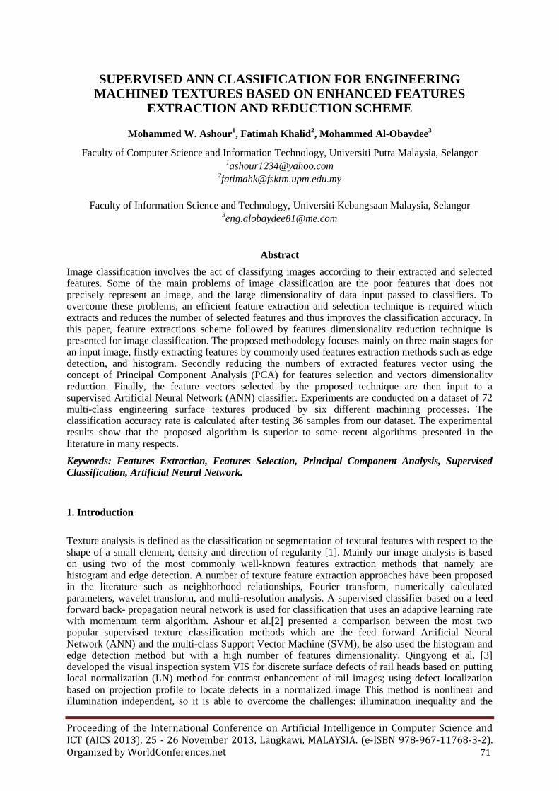
The used dataset comprises of 72 samples produced by six surface machining processes which are namely; turning, grinding, milling, lapping, and shaping [12]. Each machining process has produced twelve real samples in a class with different machines parameters (i.e. cutting speed, feed rate, and depth of cut) to give different values of roughness parameters. The milling machining process has produced twenty four samples for our dataset twelve of them are horizontally milled and the other twelve are vertically milled. This implies that our resulting dataset is of 72 samples divided into 6 classes of 12 samples for each. The samples of every class are produced by the same machining process but with different surface roughness parameter. Figure 1 illustrates two samples from each machining process from the used dataset [2].

3. Image Acquisition

This stage describes the process of converting the picture into its numerical representation, which is suitable for further image processing steps. Intensity images with 256 linear gray tones (zero corresponds to black color and 255 to white), were captured for test specimen surfaces. The surfaces were viewed under an optical microscope equipped with a digital camera. Captured images were also stored in a Personal Computer (PC) for further analysis.

This acquisition is concerned with the process of translation from light stimuli falling onto the photo sensor of camera to a stored digital value within the computer’s memory. Typically the digitized picture is up to 1024 × 1280 pixels as a spatial resolution, each pixel representation has a gray scale value. The surfaces images are viewed under a filtered optical microscope (to enhance the image) equipped with digital Charge Coupled Device (CCD) camera. The microscope used in this study is an Olympus BX51M metallurgical microscope with reflected dark light field, with several magnifications, depths of focus, and 1.2 mm

2 field of view [13].


4. Features Extraction Methods

Feature extraction is the process of creating a representation for, or a transformation from the original data. Generally there are three principal approaches used in image processing to describe the texture of a region: statistical, structural and spectral approaches [14]. In our experiment we employ two types of features, the first set of features is based on gray-level histogram, and the second one is edge detection based.

4.1. Histogram

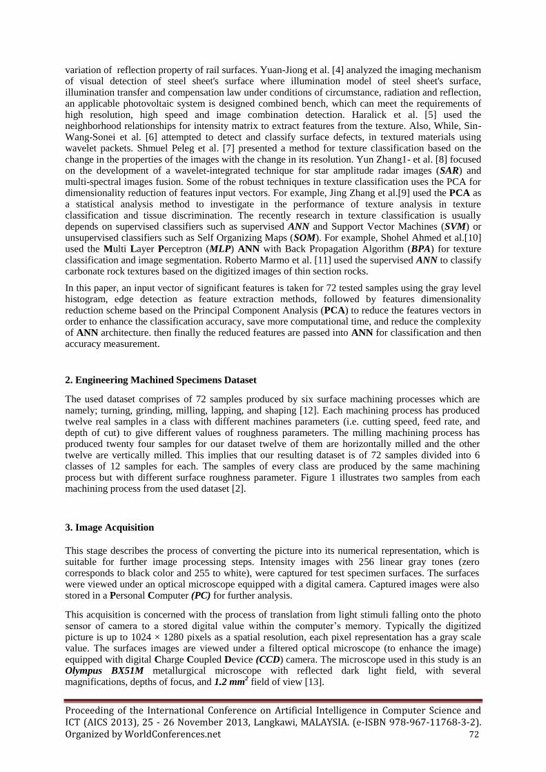
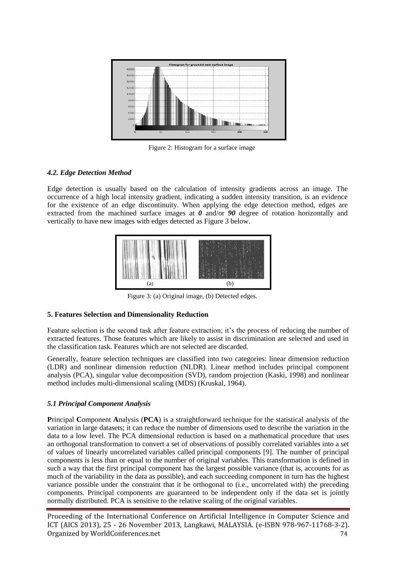
In an image processing context, the histogram of an image normally refers to a histogram of the pixel intensity values. which is a graph showing the number of pixels in an image at each different intensity value found in that image. For an 8-bit grayscale image there are 256 different possible intensities, and so the histogram will graphically display 256 numbers showing the distribution of pixels amongst those grayscale values. For intensity images, the histogram is the number of occurrences for each gray-level intensity value in an image [15]. In a graphical representation, the x-axis refers to the quantized gray-level value and the ordinate, or y-axis, refers to the number of pixels having that gray level. A monochrome value between ‘0 to 255’ of the pixel is considered as a feature for colored image.

The gray level histogram of a ground sample from our dataset is shown in Figure 2. The gray scale value (g) is obtained from the color components; red (R), green (G) and blue (B) according to the

following equation. 3

222 BGRg

(a)

(b)

(c)

(d)

(e)

Figure 1: Different machined processes samples, (a), (b), (c), (d)

and (e) are Turning, Grinding, Milling, Lapping and Shaping

respectively.

http://homepages.inf.ed.ac.uk/rbf/HIPR2/value.htm

http://homepages.inf.ed.ac.uk/rbf/HIPR2/value.htm

http://homepages.inf.ed.ac.uk/rbf/HIPR2/pixel.htm

http://homepages.inf.ed.ac.uk/rbf/HIPR2/gryimage.htm


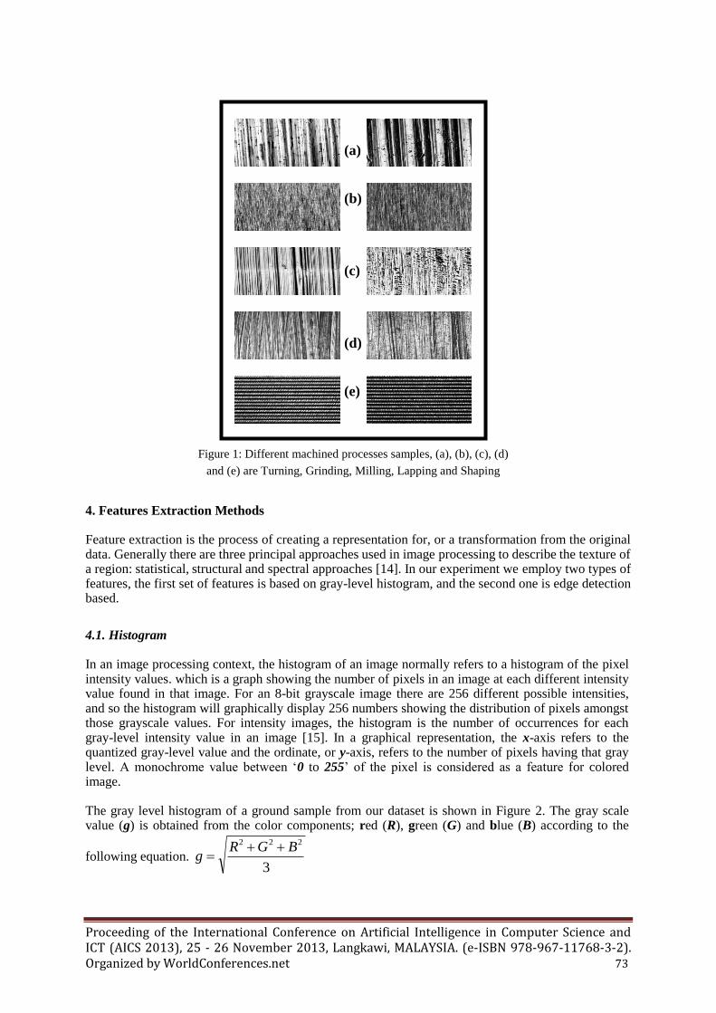
4.2. Edge Detection Method Edge detection is usually based on the calculation of intensity gradients across an image. The occurrence of a high local intensity gradient, indicating a sudden intensity transition, is an evidence for the existence of an edge discontinuity. When applying the edge detection method, edges are extracted from the machined surface images at 0 and/or 90 degree of rotation horizontally and vertically to have new images with edges detected as Figure 3 below.

5. Features Selection and Dimensionality Reduction

Feature selection is the second task after feature extraction; it’s the process of reducing the number of extracted features. Those features which are likely to assist in discrimination are selected and used in the classification task. Features which are not selected are discarded.

Generally, feature selection techniques are classified into two categories: linear dimension reduction (LDR) and nonlinear dimension reduction (NLDR). Linear method includes principal component analysis (PCA), singular value decomposition (SVD), random projection (Kaski, 1998) and nonlinear method includes multi-dimensional scaling (MDS) (Kruskal, 1964).

5.1 Principal Component Analysis

Principal Component Analysis (PCA) is a straightforward technique for the statistical analysis of the variation in large datasets; it can reduce the number of dimensions used to describe the variation in the data to a low level. The PCA dimensional reduction is based on a mathematical procedure that uses an orthogonal transformation to convert a set of observations of possibly correlated variables into a set of values of linearly uncorrelated variables called principal components [9]. The number of principal components is less than or equal to the number of original variables. This transformation is defined in such a way that the first principal component has the largest possible variance (that is, accounts for as much of the variability in the data as possible), and each succeeding component in turn has the highest variance possible under the constraint that it be orthogonal to (i.e., uncorrelated with) the preceding components. Principal components are guaranteed to be independent only if the data set is jointly normally distributed. PCA is sensitive to the relative scaling of the original variables.

Figure 2: Histogram for a surface image

Figure 3: (a) Original image, (b) Detected edges.

(a) (b)

https://en.wikipedia.org/wiki/Orthogonal_matrix

https://en.wikipedia.org/wiki/Correlation_and_dependence

https://en.wikipedia.org/wiki/Variance

https://en.wikipedia.org/wiki/Multivariate_normal_distribution#Joint_normality

https://en.wikipedia.org/wiki/Multivariate_normal_distribution#Joint_normality


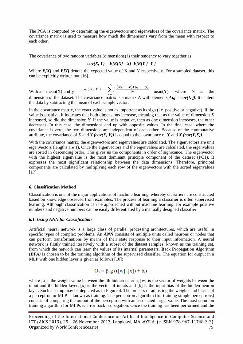
The PCA is computed by determining the eigenvectors and eigenvalues of the covariance matrix. The covariance matrix is used to measure how much the dimensions vary from the mean with respect to each other.

The covariance of two random variables (dimensions) is their tendency to vary together as:

cov(X, Y) = E[E[X] - X] E[E[Y ] -Y ]

Where E[X] and E[Y] denote the expected value of X and Y respectively. For a sampled dataset, this can be explicitly written out [16].

With = mean(X) and = mean(Y), where N is the

dimension of the dataset. The covariance matrix is a matrix A with elements Ai,j = cov(I, j). It centers the data by subtracting the mean of each sample vector.

In the covariance matrix, the exact value is not as important as its sign (i.e. positive or negative). If the value is positive, it indicates that both dimensions increase, meaning that as the value of dimension X increased, so did the dimension Y. If the value is negative, then as one dimension increases, the other decreases. In this case, the dimensions end up with opposite values. In the final case, where the covariance is zero, the two dimensions are independent of each other. Because of the commutative attribute, the covariance of X and Y (cov(X, Y)) is equal to the covariance of Y and X (cov(Y,X)).

With the covariance matrix, the eigenvectors and eigenvalues are calculated. The eigenvectors are unit eigenvectors (lengths are 1). Once the eigenvectors and the eigenvalues are calculated, the eigenvalues are sorted in descending order. This gives us the components in order of signicance. The eigenvector with the highest eigenvalue is the most dominant principle component of the dataset (PC1). It expresses the most significant relationship between the data dimensions. Therefore, principal components are calculated by multiplying each row of the eigenvectors with the sorted eigenvalues [17].

6. Classification Method

Classification is one of the major applications of machine learning, whereby classifiers are constructed based on knowledge observed from examples. The process of learning a classifier is often supervised learning. Although classification can be approached without machine learning, for example positive numbers and negative numbers can be easily differentiated by a manually designed classifier. 6.1. Using ANN for Classification

Artificial neural network is a large class of parallel processing architectures, which are useful in specific types of complex problems. An ANN consists of multiple units called neurons or nodes that can perform transformations by means of their state response to their input information. A neural network is firstly trained iteratively with a subset of the dataset samples, known as the training set, from which the network can learn the values of its internal parameters. Back Propagation Algorithm (BPA) is chosen to be the training algorithm of the supervised classifier. The equation for output in a MLP with one hidden layer is given as follows [10]:

where βi is the weight value between the ith hidden neuron, [w] is the vector of weights between the input and the hidden layer, [x] is the vector of inputs and [b] is the input bias of the hidden neuron layer. Such a set up may be depicted as in Figure 4. The process of adjusting the weights and biases of a perceptron or MLP is known as training. The perceptron algorithm (for training simple perceptrons) consists of comparing the output of the perceptron with an associated target value. The most common training algorithm for MLPs is error back propagation. Once the training has been performed and the


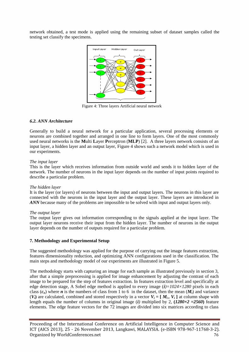
network obtained, a test mode is applied using the remaining subset of dataset samples called the testing set classify the specimens.

6.2. ANN Architecture

Generally to build a neural network for a particular application, several processing elements or neurons are combined together and arranged in one line to form layers. One of the most commonly used neural networks is the Multi Layer Perceptron (MLP) [2]. A three layers network consists of an input layer, a hidden layer and an output layer, Figure 4 shows such a network model which is used in our experiments. The input layer This is the layer which receives information from outside world and sends it to hidden layer of the network. The number of neurons in the input layer depends on the number of input points required to describe a particular problem.

The hidden layer It is the layer (or layers) of neurons between the input and output layers. The neurons in this layer are connected with the neurons in the input layer and the output layer. These layers are introduced in ANN because many of the problems are impossible to be solved with input and output layers only.

The output layer The output layer gives out information corresponding to the signals applied at the input layer. The output layer neurons receive their input from the hidden layer. The number of neurons in the output layer depends on the number of outputs required for a particular problem.

7. Methodology and Experimental Setup

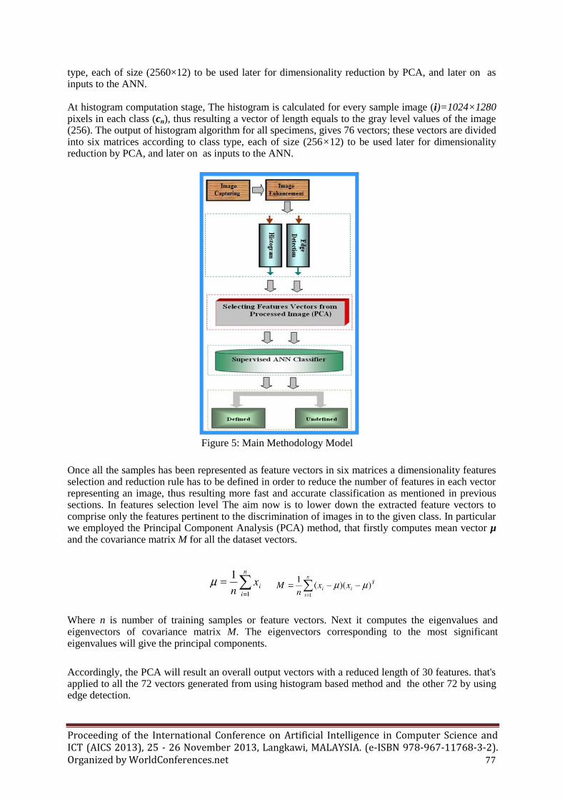
The suggested methodology was applied for the purpose of carrying out the image features extraction, features dimensionality reduction, and optimizing ANN configurations used in the classification. The main steps and methodology model of our experiments are illustrated in Figure 5.

The methodology starts with capturing an image for each sample as illustrated previously in section 3, after that a simple preprocessing is applied for image enhancement by adjusting the contrast of each image to be prepared for the step of features extraction. In features extraction level and specifically at edge detection stage, A Sobel edge method is applied to every image (i)=1024×1280 pixels in each class (cn) where n is the numbers of class from 1 to 6 in the dataset, then the mean (Mi) and variance (Vi) are calculated, combined and stored respectively in a vector Vi = [ Mi , Vi ] at column shape with length equals the number of columns in original image (i) multiplied by 2, (1280×2 =2560) feature elements. The edge feature vectors for the 72 images are divided into six matrices according to class

Figure 4: Three layers Artificial neural network


type, each of size (2560×12) to be used later for dimensionality reduction by PCA, and later on as inputs to the ANN.

At histogram computation stage, The histogram is calculated for every sample image (i)=1024×1280 pixels in each class (cn), thus resulting a vector of length equals to the gray level values of the image (256). The output of histogram algorithm for all specimens, gives 76 vectors; these vectors are divided into six matrices according to class type, each of size (256×12) to be used later for dimensionality reduction by PCA, and later on as inputs to the ANN.

Once all the samples has been represented as feature vectors in six matrices a dimensionality features selection and reduction rule has to be defined in order to reduce the number of features in each vector representing an image, thus resulting more fast and accurate classification as mentioned in previous sections. In features selection level The aim now is to lower down the extracted feature vectors to comprise only the features pertinent to the discrimination of images in to the given class. In particular we employed the Principal Component Analysis (PCA) method, that firstly computes mean vector µ and the covariance matrix M for all the dataset vectors.

Where n is number of training samples or feature vectors. Next it computes the eigenvalues and eigenvectors of covariance matrix M. The eigenvectors corresponding to the most significant eigenvalues will give the principal components.

Accordingly, the PCA will result an overall output vectors with a reduced length of 30 features. that's applied to all the 72 vectors generated from using histogram based method and the other 72 by using edge detection.

Figure 5: Main Methodology Model


In classification stage the features vectors are organized into six matrices according to class type, each of size (30 × 12), where 30 is the optimum number of reduced features and 12 is representing the number of images in a class. The first six columns of these matrices are used as the input vectors for training and the remaining six columns in that matrix are then used for testing the classifier. The used ANN configuration and parameters are listed in the following Table 1:

Table 1: Configuration and Parameters of ANN

8. Experimental Results and Discussions

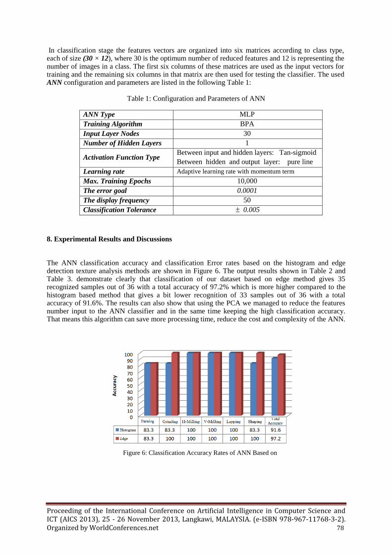
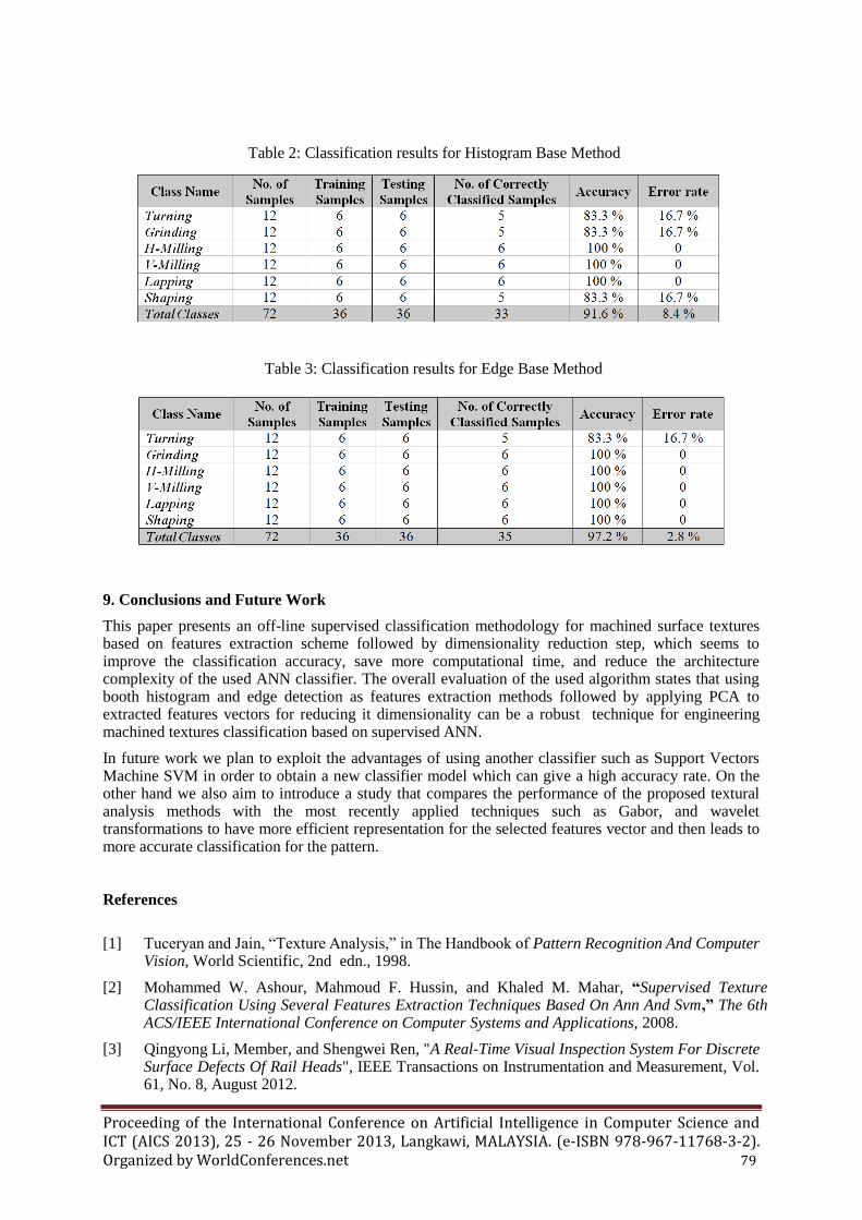
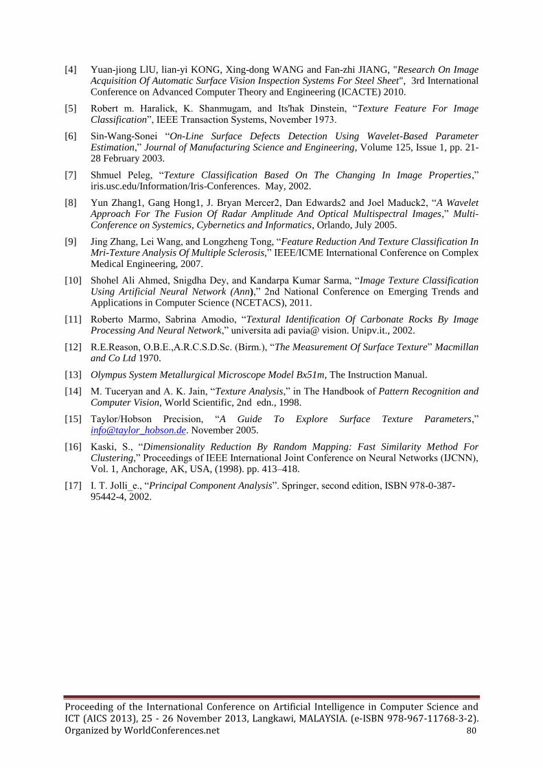
The ANN classification accuracy and classification Error rates based on the histogram and edge detection texture analysis methods are shown in Figure 6. The output results shown in Table 2 and Table 3. demonstrate clearly that classification of our dataset based on edge method gives 35 recognized samples out of 36 with a total accuracy of 97.2% which is more higher compared to the histogram based method that gives a bit lower recognition of 33 samples out of 36 with a total accuracy of 91.6%. The results can also show that using the PCA we managed to reduce the features number input to the ANN classifier and in the same time keeping the high classification accuracy. That means this algorithm can save more processing time, reduce the cost and complexity of the ANN.

ANN Type MLP

Training Algorithm BPA

Input Layer Nodes 30

Number of Hidden Layers 1

Activation Function Type Between input and hidden layers: Tan-sigmoid

Between hidden and output layer: pure line

Learning rate Adaptive learning rate with momentum term

Max. Training Epochs 10,000

The error goal 0.0001

The display frequency 50

Classification Tolerance 0.005

Figure 6: Classification Accuracy Rates of ANN Based on

Histogram and Edge Detection Methods


9. Conclusions and Future Work

This paper presents an off-line supervised classification methodology for machined surface textures based on features extraction scheme followed by dimensionality reduction step, which seems to improve the classification accuracy, save more computational time, and reduce the architecture complexity of the used ANN classifier. The overall evaluation of the used algorithm states that using booth histogram and edge detection as features extraction methods followed by applying PCA to extracted features vectors for reducing it dimensionality can be a robust technique for engineering machined textures classification based on supervised ANN.

In future work we plan to exploit the advantages of using another classifier such as Support Vectors Machine SVM in order to obtain a new classifier model which can give a high accuracy rate. On the other hand we also aim to introduce a study that compares the performance of the proposed textural analysis methods with the most recently applied techniques such as Gabor, and wavelet transformations to have more efficient representation for the selected features vector and then leads to more accurate classification for the pattern.

References

[1] Tuceryan and Jain, “Texture Analysis,” in The Handbook of Pattern Recognition And Computer

Vision, World Scientific, 2nd edn., 1998.

[2] Mohammed W. Ashour, Mahmoud F. Hussin, and Khaled M. Mahar, “Supervised Texture Classification Using Several Features Extraction Techniques Based On Ann And Svm,” The 6th ACS/IEEE International Conference on Computer Systems and Applications, 2008.

[3] Qingyong Li, Member, and Shengwei Ren, "A Real-Time Visual Inspection System For Discrete Surface Defects Of Rail Heads", IEEE Transactions on Instrumentation and Measurement, Vol. 61, No. 8, August 2012.

Table 2: Classification results for Histogram Base Method

Table 3: Classification results for Edge Base Method


[4] Yuan-jiong LlU, lian-yi KONG, Xing-dong WANG and Fan-zhi JIANG, "Research On Image Acquisition Of Automatic Surface Vision Inspection Systems For Steel Sheet", 3rd International Conference on Advanced Computer Theory and Engineering (ICACTE) 2010.

[5] Robert m. Haralick, K. Shanmugam, and Its'hak Dinstein, “Texture Feature For Image Classification”, IEEE Transaction Systems, November 1973.

[6] Sin-Wang-Sonei “On-Line Surface Defects Detection Using Wavelet-Based Parameter Estimation,” Journal of Manufacturing Science and Engineering, Volume 125, Issue 1, pp. 21-28 February 2003.

[7] Shmuel Peleg, “Texture Classification Based On The Changing In Image Properties,” iris.usc.edu/Information/Iris-Conferences. May, 2002.

[8] Yun Zhang1, Gang Hong1, J. Bryan Mercer2, Dan Edwards2 and Joel Maduck2, “A Wavelet Approach For The Fusion Of Radar Amplitude And Optical Multispectral Images,” Multi-Conference on Systemics, Cybernetics and Informatics, Orlando, July 2005.

[9] Jing Zhang, Lei Wang, and Longzheng Tong, “Feature Reduction And Texture Classification In Mri-Texture Analysis Of Multiple Sclerosis,” IEEE/ICME International Conference on Complex Medical Engineering, 2007.

[10] Shohel Ali Ahmed, Snigdha Dey, and Kandarpa Kumar Sarma, “Image Texture Classification Using Artificial Neural Network (Ann),” 2nd National Conference on Emerging Trends and Applications in Computer Science (NCETACS), 2011.

[11] Roberto Marmo, Sabrina Amodio, “Textural Identification Of Carbonate Rocks By Image Processing And Neural Network,” universita adi pavia@ vision. Unipv.it., 2002.

[12] R.E.Reason, O.B.E.,A.R.C.S.D.Sc. (Birm.), “The Measurement Of Surface Texture” Macmillan and Co Ltd 1970.

[13] Olympus System Metallurgical Microscope Model Bx51m, The Instruction Manual.

[14] M. Tuceryan and A. K. Jain, “Texture Analysis,” in The Handbook of Pattern Recognition and Computer Vision, World Scientific, 2nd edn., 1998.

[15] Taylor/Hobson Precision, “A Guide To Explore Surface Texture Parameters,” info@taylor_hobson.de. November 2005.

[16] Kaski, S., “Dimensionality Reduction By Random Mapping: Fast Similarity Method For Clustering,” Proceedings of IEEE International Joint Conference on Neural Networks (IJCNN), Vol. 1, Anchorage, AK, USA, (1998). pp. 413–418.

[17] I. T. Jolli_e., “Principal Component Analysis”. Springer, second edition, ISBN 978-0-387-95442-4, 2002.

http://iris.usc.edu/Information/Iris-Conferences.html

http://ieeexplore.ieee.org/xpl/mostRecentIssue.jsp?punumber=4381672





SUPERVISED ANN CLASSIFICATION FOR ENGINEERING MACHINED TEXTURES BASED ON ENHANCED FEATURES...

Documents

Transcript of SUPERVISED ANN CLASSIFICATION FOR ENGINEERING MACHINED TEXTURES BASED ON ENHANCED FEATURES...