Adaptive Survival Trials

Dominic Magirr1, Thomas Jaki2, Franz Koenig1, and Martin Posch1

1Section for Medical Statistics, Medical University of Vienna, Austria2Department of Mathematics and Statistics, Lancaster University, UK

May 8, 2014

arX

iv:1

405.

1569

v1 [

stat

.AP]

7 M

ay 2

014

Abstract

Mid-study design modifications are becoming increasingly accepted in confirmatory clinical trials,so long as appropriate methods are applied such that error rates are controlled. It is thereforeunfortunate that the important case of time-to-event endpoints is not easily handled by the stan-dard theory. We analyze current methods that allow design modifications to be based on the fullinterim data, i.e., not only the observed event times but also secondary endpoint and safety datafrom patients who are yet to have an event. We show that the final test statistic may ignore asubstantial subset of the observed event times. Since it is the data corresponding to the earliestrecruited patients that is ignored, this neglect becomes egregious when there is specific interest inlearning about long-term survival. An alternative test incorporating all event times is proposed,where a conservative assumption is made in order to guarantee type I error control. We examinethe properties of our proposed approach using the example of a clinical trial comparing two cancertherapies.Keywords: Adaptive design; Brownian motion; Clinical trial; Combination test; Sample sizereassessment; Time-to-event.

1 Introduction

There are often strong ethical and economic arguments for conducting interim analyses of anongoing clinical trial and for making changes to the design if warranted by the accumulatingdata. One may decide, for example, to increase the sample size on the basis of promising interimresults. Or perhaps one might wish to drop a treatment from a multi-arm study on the basis ofunsatisfactory safety data. Owing to the complexity of clinical drug development, it is not alwayspossible to anticipate the need for such modifications, and therefore not all contingencies can bedealt with in the statistical design.Unforeseen interim modifications complicate the (frequentist) statistical analysis of the trial con-siderably. Over recent decades many authors have investigated so-called “adaptive designs” inan effort to maintain the concept of type I error control (Bauer and Kohne, 1994; Proschan andHunsberger, 1995; Muller and Schafer, 2001; Hommel, 2001). Although Bayesian adaptive meth-ods are becoming increasing popular, type I error control is still deemed important in the settingof a confirmatory phase III trial (Berry et al., 2010, p. 6), and recent years have seen hybridadaptive designs proposed, whereby the interim decision is based on Bayesian methods, but thefinal hypothesis test remains frequentist (Brannath et al., 2009; Di Scala and Glimm, 2011).While the theory of adaptive designs is now well understood if responses are observed immediately,subtle problems arise when responses are delayed, e.g., in survival trials.Schafer and Muller (2001) proposed adaptive survival tests that are constructed using the inde-pendent increments property of logrank test statistics (c.f., Wassmer, 2006; Desseaux and Porcher,2007; Jahn-Eimermacher and Ingel, 2009). However, as pointed out by Bauer and Posch (2004),these methods only work if interim decision making is based solely on the interim logrank teststatistics and any secondary endpoint data from patients who have already had an event. In otherwords, investigators must remain blind to the data from patients who are censored at the interimanalysis. Irle and Schafer (2012) argue that decisions regarding interim design modifications shouldbe as substantiated as possible, and propose a test procedure that allows investigators to use thefull interim data. This methodology, similar to that of Jenkins et al. (2011), does not require anyassumptions regarding the joint distribution of survival times and short-term secondary endpoints,as do, e.g., the methods proposed by Stallard (2010), Friede et al. (2011, 2012) and Hampson andJennison (2013).The first goal of this article is to clarify the proposals of Jenkins et al. (2011) and Irle and Schafer(2012), showing that they are both based on weighted inverse-normal test statistics (Lehmacherand Wassmer, 1999), with the common disadvantage that the final test statistic may ignore asubstantial subset of the observed survival times. This is a serious limitation, as disregarding partof the observed data is generally considered inappropriate even if statistical error probabilities arecontrolled – see, for example, the discussion on overrunning in group sequential trials (Hampsonand Jennison, 2013). Our secondary goal is therefore to propose an alternative test that retainsthe strict type I error control and flexibility of the aforementioned designs, but bases the final testdecision on a statistic that takes into account all available survival times. As ever, there is nofree lunch, and the assumption that we require to ensure type I error control induces a certainamount of conservatism. We evaluate the properties of our proposed approach using the exampleof a clinical trial comparing two cancer therapies.

1

2 Adaptive Designs

2.1 Standard theory

A comprehensive account of adaptive design methodology can be found in Bretz et al. (2009). Fortesting a null hypothesis, H0 : θ = 0, against the one-sided alternative, Ha : θ > 0, the archetypaltwo-stage adaptive test statistic is of the form f1(p1) +f2(p2), where p1 is the p-value based on thefirst-stage data, p2 is the p-value from the (possibly adapted) second-stage test, and f1 and f2 areprespecified monotonically decreasing functions. Consider the simplest case that no early rejectionof the null hypothesis is possible at the end of the first stage. The null hypothesis is rejected atlevel α whenever f1(p1) + f2(p2) > k, where k satisfies∫ 1

0

∫ 1

0

1 {f1(p1) + f2(p2) ≤ k} dp1 dp2 = 1− α.

In their seminal paper, Bauer and Kohne (1994) took fi(pi) = − log(pi) for i = 1, 2. We willrestrict attention to the weighted inverse-normal test statistic (Lehmacher and Wassmer, 1999),

Z = w1Φ−1(1− p1) + w2Φ

−1(1− p2), (1)

where Φ denotes the standard normal distribution function and w1 and w2 are prespecified weightssuch that w2

1 + w22 = 1. If Z > Φ−1(1− α), then H0 may be rejected at level α. The assumptions

required to make this a valid level-α test are as follows (see Brannath et al., 2012).Assumption 1Let X int

1 denote the data available at the interim analysis, where X int1 ∈ Rn with distribution

function G(xint1 ; θ). The calendar time of the interim analysis will be denoted T int. In general,X int

1 will contain information not only concerning the primary endpoint, but also measurementson secondary endpoints and safety data. It is assumed that the first-stage p-value function p1 :Rn → [0, 1] satisfies ∫

Rn

1{p1(x

int1 ) ≤ u

}dG(xint1 ; 0) ≤ u for all u ∈ [0, 1] .

Assumption 2At the interim analysis, a second-stage design d is chosen. The second-stage design is allowed todepend on the unblinded first-stage data without prespecifying an adaptation rule. Denote thesecond-stage data by Y , where Y ∈ Rm. It is assumed that the distribution function of Y , denotedby Fd,xint1

(y, θ), is known for all possible second stage designs, d, and all first-stage outcomes, xint1 .Assumption 3The second-stage p-value function p2 : Rm → [0, 1] satisfies

∫Rm 1 {p2(y) ≤ u} dFd,xint1

(y; 0) ≤u for all u ∈ [0, 1].

2.2 Immediate responses

The aforementioned assumptions are easy to justify when primary endpoint responses are observedmore-or-less immediately. In this case X int

1 contains the responses of all patients recruited prior tothe interim analysis. A second-stage design d can subsequently be chosen with the responses froma new cohort of patients contributing to Y (Figure 1).

2

Enrollment & follow-up

X1

Enrollment & follow-up

Y

Interim Analysis Final Analysis

Calendar time

int

Figure 1: Schematic of a standard two-stage adaptive trial with immediate response.

2.3 Delayed responses and the independent increments assumption

An interim analysis may take place whilst some patients have entered the study but have yetto provide a data point on the primary outcome measure. Most approaches to this problem(e.g., Schafer and Muller, 2001; Wassmer, 2006; Jahn-Eimermacher and Ingel, 2009) attempt totake advantage of the well known independent increments structure of score statistics in groupsequential designs (Jennison and Turnbull, 2000). As pictured in Figure 2, X int

1 will generallyinclude responses on short-term secondary endpoints and safety data from patients who are yetto provide a primary outcome measure, while Y consists of some delayed responses from patientsrecruited prior to T int, mixed together with responses from a new cohort of patients.Let S(X int

1 ) and I(X int1 ) denote the score statistic and Fisher’s information for θ, calculated from

primary endpoint responses in X int1 . Assuming suitable regularity conditions, the asymptotic null

distribution of S(X int1 ) is Gaussian with mean zero and variance I(X int

1 ) (Cox and Hinkley, 1979,p. 107). The independent increments assumption is that for all first-stage outcomes xint1 andsecond-stage designs d, the null distribution of Y is such that

S(xint1 , Y )− S(xint1 ) ∼ N{

0, I(xint1 , Y )− I(xint1 )}, (2)

at least approximately, where SXint1 ,Y and IXint

1 ,Y denote the score statistic and Fisher’s information

for θ, calculated from primary endpoint responses in (X int1 , Y ).

Unfortunately, (2) is seldom realistic in an adaptive setting. Bauer and Posch (2004) show that ifthe adaptive strategy at the interim analysis is dependent on short-term outcomes in X int

1 that arecorrelated with primary endpoint outcomes in Y , i.e., from the same patient, then a naive appealto the independent increments assumption can lead to very large type I error inflation.

3

Enrollment & follow-up

X1

Enrollment & follow-up

Y

Interim Analysis

Follow-up

Follow-up

Final Analysis

Calendar time

int

Figure 2: Schematic of a two-stage adaptive trial with delayed response under the independentincrements assumption.

2.4 Delayed responses with “patient-wise separation”

An alternative approach, which we shall coin “patient-wise separation”, redefines the first-stagep-value, p1 : Rp → [0, 1], to be a function of X1, where X1 denotes all the data from patientsrecruited prior to T int, followed-up until calendar time Tmax – which corresponds to the prefixedmaximum duration of the trial. It is assumed that X1 takes values in Rp according to distributionfunction G(x1; θ). Assumption 1 is replaced with:∫

Rp

1{p1(x1) ≤ u} dG(x1; 0) ≤ u for all u ∈ [0, 1] . (3)

In this case p1 may not be observable at the time the second-stage design d is chosen. This isnot a problem, as long as no early rejection at the end of the first stage is foreseen. Any interimdecisions, such as increasing the sample size, do not require any knowledge of p1. It is assumed thatY consists of responses from a new cohort of patients, such that xint1 could be formally replacedwith x1 in assumptions 2 and 3. We call this “patient-wise separation” because data from thesame patient cannot contribute to both p1 and p2.Liu and Pledger (2005) consider such an approach for a clinical trial where a patient’s primaryoutcome is measured after a fixed period of follow-up, e.g., 4 months. Provided that one is willingto wait for all responses, it is straightforward to prespecify a first-stage p-value function such that(3) holds.For an adaptive trial with a time-to-event endpoint, however, one must be very careful to ensurethat (3) holds, as one is typically not prepared to wait for all first-stage patients – those patientsrecruited prior to T int – to have an event. Rather, p1 is defined as the p-value from an, e.g., logranktest applied to the data from first-stage patients followed up until time T1, for some T1 < Tmax. Inthis case it is vital that T1 be fixed at the start of the trial, either explicitly or implicitly (Jenkins

4

et al., 2011; Irle and Schafer, 2012). Otherwise, if T1 were to depend on the adaptive strategyat the interim analysis, this would impact the distribution of p1 and could lead to type I errorinflation.The situation is represented pictorially in Figure 3. An unfortunate consequence of prefixing T1 isthat this will not, in all likelihood, correspond to the end of follow-up for second-stage patients.All events of first-stage patients that occur after T1 make no contribution to the statistic (1); theyare “thrown away”.

Enrollment & follow-up

X1

Enrollment & follow-up

Y

Interim Analysis

Follow-up

Follow-up

Final Analysis

Unspecified follow-up

Calendar time

T1

Figure 3: Schematic of a two-stage adaptive trial with “patient-wise separation”.

3 Adaptive Survival Studies

3.1 Jenkins et al. (2011) method

Consider a randomized clinical trial comparing survival times on an experimental treatment, E,with those on a control treatment, C. We will focus on the logrank statistic for testing the nullhypothesis H0 : θ = 0 against the one-sided alternative Ha : θ > 0, where θ is the log hazard ratio,assuming proportional hazards. Let D1(t) and S1(t) denote the number of uncensored events andthe usual logrank score statistic, respectively, based on the data from first-stage patients – thosepatients recruited prior to the interim analysis – followed up until calendar time t, t ∈ [0, Tmax].Under the null hypothesis, assuming equal allocation and a large number of events, the varianceof S1(t) is approximately equal to D1(t)/4 (e.g., Whitehead, 1997, Section 3.4). The first-stagep-value must be calculated at a prefixed time point T1:

p1 = 1− Φ[2 {S1(T1)} / {D1(T1)}1/2

]. (4)

There are two possible ways of specifying T1 in (4). From a practical perspective, a calendar timeapproach is often attractive as T1 is specified explicitly, which facilitates straightforward planning.

5

On the other hand, this can produce a misspowered study if the recruitment rate and/or survivaltimes differ markedly from those anticipated. An event driven approach may be preferred, wherebythe number of events is prefixed at d1, say, and

T1 := min {t : D1(t) = d1} . (5)

Jenkins et al. (2011) describe a “patient-wise separation” adaptive survival trial, with test statistic(1), first-stage p-value (4) and T1 defined as in (5). While their focus is on subgroup selection,we will appropriate their method for the simpler situation of a single comparison, where at theinterim analysis one has the possibility to alter the pre-planned number of events from second-stagepatients – i.e., those patients recruited post T int. All that remains to be specified at the designstage is the choice of weights w1 and w2. It is anticipated that p2 will be the p-value correspondingto a logrank test based on second-stage patients, i.e.,

p2 = 1− Φ[2S2(T

∗2 )/ {D2(T

∗2 )}1/2

],

where T ∗2 := min {t : D2(t) = d∗2} with S2(t) and D2(t) defined analogously to S1(t) and D1(t),and d∗2 is to be specified at the interim analysis. Ideally, the weights should be chosen in pro-portion to the information (number of events) contributed from each stage. In an adaptive trial,it is impossible to achieve the correct weighting in every scenario. Jenkins et al. prespecify theenvisioned number of second-stage events, d2, and choose weights w1 = {d1/(d1 + d2)}1/2 and

w2 = {d2/(d1 + d2)}1/2.

3.2 Irle and Schafer (2012) method

Irle and Schafer (2012) propose an alternative procedure. Instead of explicitly combining stage-wisep-values, they employ the closely related conditional error approach (Proschan and Hunsberger,1995; Posch and Bauer, 1999; Muller and Schafer, 2001).They begin by prespecifying a level-α test with decision function, ϕ, taking values in {0, 1} cor-responding to nonrejection and rejection of H0, respectively. For a survival trial, this entailsspecifying the sample size, duration of follow-up, test statistic, recruitment rate, etc. Then, atsome (not necessarily prespecified) timepoint, T int, an interim analysis is performed. The timingof the interim analysis induces a partition of the trial data, (X1, X2), where X1 and X2 denote thedata from patients recruited prior- T int and post- T int, respectively, followed-up until time Tmax.More specifically, Irle and Schafer (2012) suggest the decision function

ϕ(X1, X2) = 1[2S1,2(T1,2)/ {D1,2(T1,2)}1/2 > Φ−1(1− α)

], (6)

where D1,2(T1,2) and S1,2(T1,2) denote the number of uncensored events and the usual logrank scorestatistic, respectively, based on data from all patients (from both stages) followed-up until timeT1,2, where T1,2 := min {t : D1,2(t) = d1,2} for some prespecified number of events d1,2.At the interim analysis, the general idea is to use the unblinded first-stage data xint1 to definea second-stage design, d, without the need for a prespecified adaptation strategy. Again, thedefinition of d includes factors such as sample size, follow-up period, recruitment rate, etc., inaddition to a second-stage decision function ψxint1

: Rm → {0, 1} based on second-stage data

6

Y ∈ Rm. Irle and Schafer (2012) focus their attention on a specific design change; namely, thepossibility of increasing the number of events from d1,2 to d∗1,2 by extending the follow-up period.They assume that Y := (X1, X2) \X int

1 and propose the second-stage decision function

ψxint1(Y ) = 1

[2S1,2(T

∗1,2)/

{D1,2(T

∗1,2)}1/2 ≥ b∗

], (7)

where T ∗1,2 := min{t : D1,2(t) = d∗1,2

}and b∗ is a cutoff value that must be determined. Ideally,

one would like to choose b∗ such that EH0(ψXint1| X int

1 = xint1 ) = EH0(ϕ | X int1 = xint1 ), as this would

ensure that

EH0(ψXint1

) = EH0

{EH0

(ψXint

1| X int

1

)}= EH0

{EH0

(ϕ | X int

1

)}= EH0(ϕ) = α, (8)

i.e., the overall procedure controls the type I error rate at level α. Unfortunately, this approachis not directly applicable in a survival trial where X int

1 contains short-term data from first-stagepatients surviving beyond T int. This is because it is impossible to calculate EH0(ϕ | X int

1 = xint1 )and EH0(ψXint

1| X int

1 = xint1 ), owing to the unknown joint distribution of survival times and thesecondary/safety endpoints already observed at the interim analysis, c.f. Section 2.3. Irle andSchafer (2012) get around this problem by conditioning on additional variables; namely, S1(T1,2)and S1(T

∗1,2). Choosing ψxint1

such that

EH0

{ψXint

1| X int

1 = xint1 , S1(T1,2) = s1, S1(T∗1,2) = s∗1

}= EH0

{ϕ | X int

1 = xint1 , S1(T1,2) = s1, S1(T∗1,2) = s∗1

}ensures that EH0(ψXint

1) = α following the same argument as (8).

Irle and Schafer (2012) show that, asymptotically,

EH0

{ϕ | X int

1 = xint1 , S1(T1,2) = s1, S1(T∗1,2) = s∗1

}= EH0 {ϕ | S1(T1,2) = s1}

and

EH0

{ψXint

1| X int

1 = xint1 , S1(T1,2) = s1, S1(T∗1,2) = s∗1

}= EH0

{ψxint1

| S1(T∗1,2) = s∗1

}.

In each case, calculation of the right-hand-side is facilitated by the asymptotic result that, assumingequal allocation under the null hypothesis,(

S1(t)S1,2(t)− S1(t)

)∼ N

((00

),

(D1(t)/4 0

0 {D1,2(t)−D1(t)} /4

)), (9)

for t ∈ [0, T ], where T is sufficiently large such that all events of interest occur prior to T .

One remaining subtlety is that EH0

{ψxint1

| S1(T∗1,2) = s1

}can only calculated at calendar time

T ∗1,2, where T ∗1,2 > T int. Determination of b∗ must therefore be postponed until this later time.It is shown in Appendix A that ψXint

1= 1 if and only if Z > Φ−1(1− α), where Z is defined as in

(1) with p1 defined as in (4), T1 defined as equal to T1,2, the second-stage p-value function definedas

p2(Y ) = 1− Φ[2{S1,2(T

∗1,2)− S1(T

∗1,2)}/{d∗1,2 −D1(T

∗1,2)}1/2]

, (10)

and the specific choice of weights:

w1 = {D1(T1,2)/d1,2}1/2 and w2 = [{d1,2 −D1(T1,2)} /d1,2]1/2 . (11)

7

Remark 1. In a sense, the Irle and Schafer method can be thought of as a special case of theJenkins et al. method, with a clever way of implicitly defining the weights and the end of first-stagefollow-up, T1. It has two potential advantages. Firstly, the timing of the interim analysis need notbe prespecified – in theory, one is permitted to monitor the accumulating data and at any momentdecide that design changes are necessary. Secondly, if no changes to the design are necessary, i.e.,the trial completes as planned at calendar time T1,2, then the original test (6) is performed. Inthis special case, no data is “thrown away”.Remark 2. From first glance at (7), it may appear that the data from first-stage patients,accumulating after T1,2, is never “thrown away”. However, this data is still effectively ignored. Wehave shown that the procedure is equivalent to a p-value combination approach where p1 dependsonly on data available at time T1 := T1,2. In addition, the distribution of p2 is asymptoticallyindependent of the data from first-stage patients: note that S1,2(T

∗1,2) − S1(T

∗1,2) and S2(T

∗1,2) are

asymptotically equivalent (Irle and Schafer, 2012, remark 1). The procedure therefore fits ourdescription of a “patient-wise separation” design, c.f. Section 2.4, and the picture is the sameas in Figure 3. The first-stage patients have in effect been censored at T1,2, despite having beenfollowed-up for longer.This fact has important implications for the choice of d∗1,2. If one chooses d∗1,2 based on conditionalpower arguments, one should be aware that the effective sample size has not increased by d∗1,2−d1,2.Rather, it has increased by d∗1,2− d1,2−

{D1(T

∗1,2)−D1(T1,2)

}, which could be very much smaller.

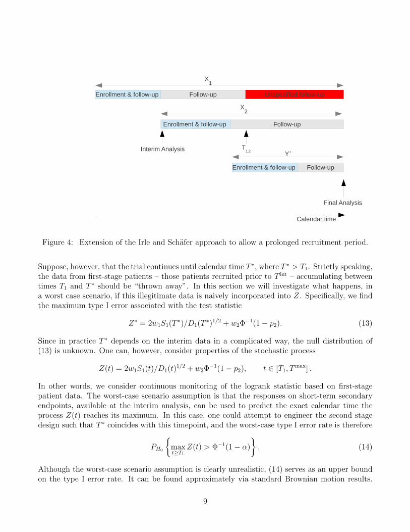
Remark 3. A potential disadvantage of the Irle and Schafer (2012) method is that it is not possibleto decrease the number of events (nor decrease the recruitment rate) at the interim analysis, asone must observe at least d1,2 events (in the manner specified by the original design) to be able tocalculate the conditional error probability EH0 {ϕ | S1(T1,2)}.In addition, one is not permitted to increase the recruitment rate following the interim analysis, norto prolong the recruitment period beyond that prespecified by the original design. In order to allowsuch design changes, a small extension is necessary. While the conditional error probability remainsEH0 {ϕ | S1(T1,2)}, the second-stage data must be split into two parts, Y =

{(X1, X2) \X int

1 , Y +}

,where Y + consists of responses from an additional cohort of patients, not specified by the originaldesign (see Figure 4). The second-stage test (7) can be replaced with, e.g.,

ψxint1(Y ) = 1

[2S2,+(T2,+)/ {D2,+(T2,+)}1/2 ≥ b∗

],

where D2,+(T2,+) and S2,+(T2,+) are the observed number of events and the usual logrank scorestatistic, respectively, based on the responses of all patients recruited post T int, and T2,+ :=min {t : D2,+(t) = d2,+} for some d2,+ defined at time T int. Again, determination of b∗ must bepostponed until time max(T1,2, T2,+).

3.3 Effect of unspecified follow-up data

Continuing with the set up and notation of Section 3.1 (which we have shown also fits the Irle andSchafer (2012) method), the adaptive test statistic is

Z = w1Φ−1(1− p1) + w2Φ

−1(1− p2)= 2w1S1(T1)/D1(T1)

1/2 + w2Φ−1(1− p2). (12)

8

Enrollment & follow-up

X1

Enrollment & follow-up

X2

Interim Analysis

Follow-up

Follow-up

Final Analysis

Unspecified follow-up

Enrollment & follow-up Follow-up

T1,2

Y+

Calendar time

Figure 4: Extension of the Irle and Schafer approach to allow a prolonged recruitment period.

Suppose, however, that the trial continues until calendar time T ∗, where T ∗ > T1. Strictly speaking,the data from first-stage patients – those patients recruited prior to T int – accumulating betweentimes T1 and T ∗ should be “thrown away”. In this section we will investigate what happens, ina worst case scenario, if this illegitimate data is naively incorporated into Z. Specifically, we findthe maximum type I error associated with the test statistic

Z∗ = 2w1S1(T∗)/D1(T

∗)1/2 + w2Φ−1(1− p2). (13)

Since in practice T ∗ depends on the interim data in a complicated way, the null distribution of(13) is unknown. One can, however, consider properties of the stochastic process

Z(t) = 2w1S1(t)/D1(t)1/2 + w2Φ

−1(1− p2), t ∈ [T1, Tmax] .

In other words, we consider continuous monitoring of the logrank statistic based on first-stagepatient data. The worst-case scenario assumption is that the responses on short-term secondaryendpoints, available at the interim analysis, can be used to predict the exact calendar time theprocess Z(t) reaches its maximum. In this case, one could attempt to engineer the second stagedesign such that T ∗ coincides with this timepoint, and the worst-case type I error rate is therefore

PH0

{maxt≥T1

Z(t) > Φ−1(1− α)

}. (14)

Although the worst-case scenario assumption is clearly unrealistic, (14) serves as an upper boundon the type I error rate. It can be found approximately via standard Brownian motion results.

9

Define the information time at calendar time t to be u = D1(t)/D1(Tmax), and let S1(u) denote

the logrank score statistic based on first-stage patients, followed-up until information time u. Itcan be shown that B(u) := 2S1(u)/ {D1(T

max)}1/2 behaves asymptotically like a Brownian motion

with drift ξ := θ {D1(Tmax)/4}1/2 (Proschan et al., 2006, p. 101).

We wish to calculate

Pθ=0

{maxt≥T1

Z(t) > Φ−1(1− α)

}=

∫ 1

0

Pθ=0

[1

maxu=u1

B(u) > u1/2w−11

{Φ−1(1− α)− w2Φ

−1(1− p2)}]

dp2,

(15)where u1 = D1(T1)/D1(T

max). While the integrand on the right-hand-side is difficult to evaluateexactly, it can be found to any required degree of accuracy by replacing the square root stoppingboundary with a piecewise linear boundary (Wang and Potzelberger, 1997). Some further detailsare provided in Appendix B.The two parameters that govern the size of (14) are w1 and u1. Larger values of w1 reflect anincreased weighting of the first-stage data, which increases the potential inflation. In addition, alow value for u1 increases the window of opportunity for stopping on a random high. Figure 5shows that for a nominal α = 0.025 level test, the worst-case type I error can be up to 15% whenu1 = 0.1 and w1 = 0.9. As u1 → 0 the worst-case type I error rate tends to 1 for any value of w1

(see, e.g., Proschan et al., 1992).

0.2 0.4 0.6 0.8

0.2

0.4

0.6

0.8

u1

w1

0.04

0.06

0.08

0.10

0.12

0.14

Figure 5: Worst case type I error for various choices of weights and information fractions.

10

4 Example

The upper bound on the type I error rate, as depicted in Figure 5, varies substantially across w1

and u1. The following example, simplified from Irle and Schafer (2012), is intended to give anindication of what can be expected in practice.A randomized trial is set up to compare chemotherapy (C) with a combination of radiotherapyand chemotherapy (E). The anticipated median survival time on C is 14 months. If E were toincrease the median survival time to 20 months then this would be considered a clinically relevantimprovement. Assuming exponential survival times, this gives anticipated hazard rates λC = 0.050and λE = 0.035, and a target log hazard ratio of θR = − log(λE/λC) = 0.36. If the error rates fortesting H0 : θ = 0 against Ha : θ = θR are α = 0.025 (one-sided) and β = 0.2, the required numberof deaths (assuming equal allocation) is

d1,2 = 4[{

Φ−1(1− α) + Φ−1(1− β)}/θR]2 ≈ 248.

If 8 patients per month are recruited at a uniform rate throughout an initial period of 40 months,and the survival times of these patients are followed-up for an additional 20 months after the endof this period, then standard sample size formulae (Machin et al., 1997, Section 9.2.3.) tell us wecan expect to observe around 250 deaths by the time of the final analysis.Now imagine, as Irle and Schafer (2012) did, that an interim look is performed after 60 deaths,observed 23 months after the start of the trial. At this point in time, 190 patients have beenrecruited. Based on the interim results, it is decided to increase the total required number ofevents from d1,2 to d∗1,2.At the time of the 248th death, i.e., the originally planned study end T1,2, suppose we observethat 170 of these deaths have come from patients recruited prior to the interim look. We have ourweights (11),

w1 = (170/248)1/2 and w2 = (78/248)1/2.

At this point we make a note of the standardized first-stage logrank score statistic S1(T1) :=S1(T1,2) and hence p1 from (4), and continue to follow-up survival times until a total of d∗1,2 deathshave been observed. Once these additional deaths have been observed, p2 can be found from (10),and combined with p1 to give the adaptive test statistic (1).Notice that w1 = (170/248)1/2 and, ignoring any potential censoring, u1 = D1(T1)/D1(T

max) =170/190. In this case a naive application of the test statistic (13) leads to an upper bound on thetype I error rate of 0.040. The inflation is not enormous, owing to the relatively slow recruitmentrate, but it is not hard to imagine more worrying scenarios.Suppose, for example, that the trial design called for 48 patients to be recruited per month for12 months, with 8 months of additional follow-up. Further suppose that an interim analysis tookplace 6 months into the trial, by which time 288 patients had been recruited, and a decision wasmade to increase the total number of events. Given the anticipated λC and λE, a plausible scenariois that 147 of the first 248 events come from first-stage patients, implying that w1 = (147/248)1/2

and u1 = 147/288. This gives an upper bound (14) of 0.066.

4.1 An alternative level-α test

A possible rationale for using (13), instead of (12), is that the final test statistic takes into accountall available survival times, i.e., does not ignore any data. If one is unprepared to give up the

11

guarantee of type I error control, an alternative test can be found by increasing the cut-off valuefor Z∗ from Φ−1(1− α) to k∗ such that∫ 1

0

Pθ=0

[1

maxu=u1

B(u) > u1/2w−11

{k∗ − w2Φ

−1(1− p2)}]

dp2 = α

This will, of course, have a knock on effect on power. Table 1 gives an impression of how muchthe cutoff is increased from 1.96 when α = 0.025 (one sided).

Table 1: Cutoff values for corrected level-0.025 test.

u10.1 0.2 0.3 0.4 0.5 0.6 0.7 0.8 0.9

0.1 2.29 2.25 2.21 2.19 2.16 2.13 2.11 2.08 2.040.2 2.41 2.35 2.31 2.27 2.23 2.20 2.16 2.12 2.070.3 2.50 2.43 2.38 2.34 2.30 2.25 2.21 2.16 2.100.4 2.58 2.50 2.44 2.39 2.34 2.30 2.25 2.19 2.12

w1 0.5 2.64 2.56 2.49 2.44 2.38 2.33 2.27 2.21 2.140.6 2.70 2.60 2.53 2.47 2.42 2.36 2.30 2.23 2.150.7 2.74 2.64 2.57 2.51 2.45 2.39 2.33 2.26 2.170.8 2.79 2.68 2.60 2.54 2.48 2.41 2.35 2.28 2.180.9 2.83 2.72 2.64 2.57 2.50 2.43 2.37 2.29 2.19

In assessing the effect on power, at least four probabilities appear relevant:

A. Pθ=θR

[2w1S1(T1)/ {D1(T1)}1/2 + w2Φ

−1(1− p2) > Φ−1(1− α)].

B. Pθ=θR

[2w1S1(T1)/ {D1(T1)}1/2 + w2Φ

−1(1− p2) > k∗].

C. Pθ=θR

[2w1S1(T

max)/ {D1(Tmax)}1/2 + w2Φ

−1(1− p2) > k∗].

D. Pθ=θR {maxt≥T1 Z(t) > k∗}.

Power definition A corresponds to the “correct” adaptive test. B can be thought of as a lowerbound on the power of the alternative level-α test, where one conscientiously specifies the increasedcutoff value k∗ (in anticipation of unpredictable end of first-stage follow-up), but it then turns outthat the trial finishes at the prespecified time point anyhow, i.e., T ∗ = T1. Definition C canbe thought of as the power of the alternative test if the trial is always prolonged such that allfirst-stage events are observed. Definition D, on the other hand, can be interpreted as the powerof the alternative level-α test, taken at face value. In other words, assuming that one takes theopportunity to stop follow-up of first-stage patients when Z(t) is at its maximum. This can becalculated using the same techniques as in Section 3.3.Figure 6 shows the power of the trial described in Example 4, according to A-D. The power hasbeen evaluated conditional on p2, as this is a random variable common to all four definitions. Theincreased cutoff value of the alternative level-α test leads to a sizeable loss of power if the trialcompletes as planned. In the second scenario at least, the loss of power can be more than made up

12

0.0 0.2 0.4 0.6 0.8 1.0

0.0

0.2

0.4

0.6

0.8

1.0

p2

Pow

er

(a)

0.0 0.2 0.4 0.6 0.8 1.0

0.0

0.2

0.4

0.6

0.8

1.0

p2

Pow

er

(b)

Figure 6: Conditional power as defined by A (thin line), B (medium line), C (thick line) and Dy(dashed line) given p2, under the two scenarios described in Example 4. Scenario (a): D1(T1) = 170,D1(T

max) = 190, w1 = (170/248)1/2 and θR = 0.36. Scenario (b): D1(T1) = 147, D1(Tmax) = 288,

w1 = (147/248)1/2 and θR = 0.36.

for when the trial is prolonged. However, if there is an a-priori reasonable probability of prolongingthe trial, then one could just start with a larger sample size/ required number of events.In general, the differences between power definitions A-D will tend to follow the same patternas in Figure 6. The degree to which they differ will depend on w1, D1(T1), D1(T

max) and θR.Intuitively, larger w1 and smaller u1 will lead to a greater loss of power going from A to B, butwith a greater potential gain in power going from B to C (or D). The actual gain in power fromB to C (or D) will be greatest for large values of θR

4.2 Diverging hazard rates

Consider the second trial design in Section 4, where recruitment proceeds at a uniform rate of 48patients per month for 12 months, with 8 months of additional follow-up. Suppose, however, thatthe true hazard rates are not proportional. Rather, hE(τ) = 0.04 and h−1C (τ) = 0.04−1 − 0.6τfor τ ∈ (0, 30), where τ denotes the time in calendar months since randomization. Simulating arealization of this trial, 295 patients are recruited in the first six months, by which time there havebeen 18 deaths on C, and 15 deaths on E. Suppose that at this point it is decided to increase thetarget number of events from d1,2 = 248 to d∗1,2 = 350. At time T1,2, the number of deaths fromfirst-stage patients – those patients recruited in the first six months – is D1(T1,2) = 151, such thatw1 = (151/248)1/2, u1 = 151/295 and k∗ = 2.41. The logrank score statistics based on first-stagepatients is S1(T1,2) = 7.6, giving a first-stage p-value (4) of

p1 = 1− Φ{

2(7.6)/1511/2}

= 0.108

13

and a conditional error probability (6) of EH0 {ϕ | S1(T1,2) = 7.6} = 0.213, using (9).The survival data at time T ∗1,2, occurring approximately 26 months into the trial, is plotted inFigure 7. On the left-hand-side, all survival times have been included in the Kaplan-Meier curves.There is an obvious divergence in the survival probabilities on the two treatments. However, thetest decision of Irle and Schafer (2012) may only use the data as depicted on the right-hand-side,where the survival times of first-stage patients have been censored at time T1,2. They are liable toreach an inappropriate conclusion. In this case, 199 out of the first 350 events are from patientsrecruited in the first six months, and the logrank score statistic based on first-stage patients isS1(T

∗1,2) = 16. The new cutoff value b∗ must be found to solve

EH0

{ψxint1

| S1(T∗1,2) = 16

}= PH0

{2S1,2(T

∗1,2)/3501/2 ≥ b∗ | S1(T

∗1,2) = 16

}= 0.213,

which gives b∗ = 2.76, using (9). The logrank statistic based on all survival times at T ∗1,2 isS1,2(T

∗1,2) = 25 and the test decision is

ψxint1= 1

{2(25)/3501/2 ≥ 2.76

}= 0,

i.e., one cannot reject the null hypothesis. As shown in Section 3.2, the same decision could havebeen reached by finding the second-stage p-value (10)

p2 = 1− Φ[2 {25− 16} /(350− 199)1/2

]= 0.071,

computing the adaptive test statistic (1),

Z = w1Φ−1(1− p1) + w2Φ

−1(1− p2) = 1.88,

and comparing with Φ−1(1− α) ≈ 1.96. The number of events that have been ignored in makingthis decision is D1(T

∗1,2)−D1(T1,2) = 48.

If, on the other hand, one had prespecified the alternative test of Section 4.1, then one would bepermitted to replace Φ−1(1− p1) in the adaptive test statistic with the value of the standardizedlogrank statistic at time T ∗1,2. In this case one would be able to reject the null hypothesis, as

Z(T ∗1,2) = 2w1S1(T∗1,2)/D1(T

∗1,2)

1/2 + w2Φ−1(1− p2) = 2.69 > k∗.

5 Discussion

Adaptive design methodology – developed over the past two decades to cope with mid-studyprotocol changes in confirmatory clinical trials – is becoming increasingly accepted by regulatoryagencies (Elsaesser et al., 2013). It is therefore unfortunate that the important case of time-to-event data is not easily handled by the standard theory. As far as survival data are concerned,all proposed solutions have limitations and there is a trade-off between strict type I error control,power, flexibility, the use of all interim data to substantiate interim decision making, and the useof all available data in making the test decision at the final analysis.The proposed solutions of Irle and Schafer (2012) and Jenkins et al. (2011) offer strict type I errorcontrol and allow full use of the interim data. The Jenkins et al. (2011) method allows one to

14

0 5 10 15 20 25

0.0

0.2

0.4

0.6

0.8

1.0

Months since randomization

Sur

viva

l pro

babi

lity

ControlExperimental

(a)

0 5 10 15 20 25

0.0

0.2

0.4

0.6

0.8

1.0

Months since randomization

Sur

viva

l pro

babi

lity

ControlExperimental

(b)

Figure 7: Kaplan-Meier plots corresponding to the hypothetical trial described in Section 4.2based on (a) all available survival times at T ∗1,2, and (b) with first-stage and second-stage patientscensored at T1,2 and T ∗1,2, respectively.

change the recruitment rate at the interim analysis – something that is disallowed by Irle andSchafer (2012), where one is only permitted to increase the observation time. On the other hand,Irle and Schafer (2012) is more flexible in the sense that the timing of the interim analysis neednot be prespecified. In both cases, the final test decision only depends on a subset of the recordedsurvival times, i.e., part of the observed data is ignored. This is usually deemed unacceptable byregulators. Furthermore, it is the long-term data of patients recruited prior to the interim analysisthat is ignored, such that more emphasis is put on early events in the final decision making. Thisneglect becomes egregious when there is specific interest in learning about the long-term parts ofthe survival curves.We have therefore proposed an alternative procedure which offers the same type I error control andflexibility as Jenkins et al. (2011) and Irle and Schafer (2012), in addition to a final test statisticthat takes into account all available survival times. However, in order to achieve this, a worst-caseadjustment is made a-priori in the planning phase. If no design modifications are performed atthe interim analysis, the worst-case critical boundary must nevertheless be applied. This resultsin a loss of power.Methods based on the independent increments assumption have been only briefly mentioned inSection 2.3. They suffer from the limitation that decision makers must be blinded to short-termdata at the interim analysis. On the other hand, subject to this blinding being imposed, the typeI error rate is controlled and the final test decision is based on all available survival times. Thiscould therefore be a viable option in situations where the short-term data is sparse or relativelyuninformative. Yet another option, if one is prepared to give up strict type I error control, issimply to use the usual logrank test at the final analysis. The true operating characteristics ofsuch a procedure are unclear, owing to the complex dependence on the interim data.Our alternative level-α test may have practical applications in multi-arm survival trials (Jaki and

15

Magirr, 2013) and adaptive enrichment designs. In this case, one must take great care in applyingthe methodology of Jenkins et al. (2011) or Irle and Schafer (2012). One specific issue is thatdropping a treatment arm will affect recruitment rates on other arms. Also, for treatment regimesthat have to be given continuously over a period of time, it would be unethical to keep treatingpatients on treatment arms that have been dropped for futility. This may affect the timing ofanalyses on other arms. Incorporating some flexibility into the end of patient follow-up couldconfer advantages here. More research is needed in this area.The usefulness of performing design modifications has to be thoroughly assessed on a case-by-casebasis in the planning phase. Interim data may be highly variable, and the interim survival resultsmay be driven mainly by early events. Consequently, the interim data may be too premature toallow a sensible interpretation of the whole survival curves and may not be a reliable basis foradaptations.In this respect, the best advice might be to thoroughly assess the characteristics of adaptive trialdesigns in comparison with more standard approaches, and to plan for adaptations only in settingswhere the advantages are compelling. If in the planning phase there is a strong likelihood thatthe number of patients will need to be increased, or the observation time extended, our analysishas shown that there is no uniformly best design. All proposals to implement adaptive survivaldesigns have their limitations. If the main objective is strict type I error control when using alldata, then our proposal should be considered as a valid option.

Appendix A

Connection between conditional error and combination test

The cut-off b∗ satisfies

EH0 {ϕ | S1(T1,2) = s1} = PH0

{2S1,2(T

∗1,2)/(d

∗1,2)

1/2 ≥ b∗ | S1(T∗1,2) = s∗1

}= PH0

[2{S1,2(T

∗1,2)− S1(T

∗1,2)}/{d∗1,2 −D1(T

∗1,2)}1/2 ≥ c∗ | S1(T

∗1,2) = s∗1

],

which implies that c∗ = Φ−1 [1− EH0 {ϕ | S1(T1,2) = s1}], using (9). Therefore,

ψXint1

= 1⇔ 2S1,2(T∗1,2)/(d

∗1,2)

1/2 ≥ b∗

⇔ 2{S1,2(T

∗1,2)− S1(T

∗1,2)}/{d∗1,2 −D1(T

∗1,2)}1/2 ≥ c∗

⇔ Φ−1(1− p2) ≥ Φ−1 [1− EH0 {ϕ | S1(T1,2) = s1}]⇔ p2 ≤ EH0 {ϕ | S1(T1,2) = s1} .

The conditional error probability, EH0 {ϕ | S1(T1,2) = s1}, can be found from the joint distribution(9) at calendar time T1,2. Omitting the argument T1,2 from S1, S1,2, D1 and D1,2:

EH0 {ϕ | S1 = s1} = PH0

{2S1,2/(D1,2)

1/2 > Φ−1(1− α) | S1 = s1

}= PH0

[2(S1,2 − S1)/(D1,2 −D1)

1/2 > Φ−1(1− α) {D1,2/(D1,2 −D1)}1/2

−2S1/(D1,2 −D1)1/2 | S1 = s1

]= 1− Φ

[Φ−1(1− α) {D1,2/(D1,2 −D1)}1/2 − Φ−1(1− p1) {D1/(D1,2 −D1)}1/2

]16

and therefore p2 ≤ EH0 {ϕ | S1(T1,2) = s1} if and only if

{D1(T1,2)/d1,2}1/2 Φ−1(1− p1) + [{d1,2 −D1(T1,2)} /d1,2]1/2 Φ−1(1− p2) ≥ Φ−1(1− α).

Appendix B

Computation of (14)

For simplicity, consider replacing the square root boundary in (15) with a linear boundary. Con-ditional on p2, our problem is to find Pθ=0 {B(u) < au+ b, u1 < u ≤ 1}, where a and b are foundby drawing a line through

u1, u1/21 w−11

{Φ−1(1− α)− w2Φ

−1(1− p2)}

and1, w−11

{Φ−1(1− α)− w2Φ

−1(1− p2)}.

For constants a, b and c, with b, c > 0, Siegmund (1986) shows that

Pθ=0 {B(u) ≥ au+ b, for some 0 < u ≤ c | W (c) = x} = exp {−2b(ac+ b− x)/c}

and integrating over x gives

Pθ=0 {B(u) < au+ b, u ≤ c} = Φ{

(ac+ b)/c1/2}− exp(−2ab)Φ

{(ac− b)/c1/2

}. (16)

Therefore, conditioning on the value of B(u1),

Pθ=0 {B(u) < au+ b, u1 < u ≤ 1} =

∫ au1

−∞Pθ=0 {B(u) < au+ b, u1 < u ≤ 1 | B(u1) = x} dPu1(x; 0)

=

∫ au1

−∞Pθ=0 {B(u+ u1)− x

< a(u+ u1) + b− x, 0 < u ≤ 1− u1 | B(u1) = x} dPu1(x; 0)

=

∫ au1

−∞Pθ=0 {B(v) < av + au1 + b− x, 0 < v ≤ 1− u1} dPu1(x; 0)

=

∫ au1

−∞Φ

{a+ b− x

(1− u1)1/2

}− exp {−2a(au1 + b− x)}Φ

{a(1− 2u1)− b+ x

(1− u1)1/2

}dPu1(x; 0).

Greater accuracy can be achieved by replacing the square root boundary with a piece-wise linearboundary, in which case one must condition on the value of the Brownian motion at each of thecut-points (Wang and Potzelberger, 1997).

17

References

Bauer, P. and Kohne, K. (1994). Evaluation of experiments with adaptive interim analyses. Bio-metrics, 50:1029–1041. Correction: Biometrics 1996; 52:380.

Bauer, P. and Posch, M. (2004). Letter to the editor. Statistics in Medicine, 23:1333–1334.

Berry, S. M., Carlin, B. P., Lee, J. J., and Muller, P. (2010). Bayesian adaptive methods for clinicaltrials. CRC press.

Brannath, W., Gutjahr, G., and Bauer, P. (2012). Probabilistic foundation of confirmatory adap-tive designs. Journal of the American Statistical Association, 107:824–832.

Brannath, W., Zuber, E., Branson, M., Bretz, F., Gallo, P., Posch, M., and Racine-Poon, A.(2009). Confirmatory adaptive designs with bayesian decision tools for a targeted therapy inoncology. Statistics in medicine, 28(10):1445–1463.

Bretz, F., Koenig, F., Brannath, W., Glimm, E., and Posch, M. (2009). Adaptive designs forconfirmatory clinical trials. Statistics in Medicine, 28:1181–1217.

Cox, D. R. and Hinkley, D. V. (1979). Theoretical statistics. CRC Press.

Desseaux, K. and Porcher, R. (2007). Flexible two-stage design with sample size reassessment forsurvival trials. Statistics in medicine, 26(27):5002–5013.

Di Scala, L. and Glimm, E. (2011). Time-to-event analysis with treatment arm selection at interim.Statistics in medicine, 30(26):3067–3081.

Elsaesser, A., Regnstroem, J., Vetter, T., Koenig, F., Hemmings, R., Greco, M., Papaluca-Amati,M., and Posch, M. (2013). Adaptive designs in european marketing authorisation a survey ofadvice letters at the european medicines agency. Submitted.

Friede, T., Parsons, N., and Stallard, N. (2012). A conditional error function approach for subgroupselection in adaptive clinical trials. Statistics in Medicine, 31(30):4309–4320.

Friede, T., Parsons, N., Stallard, N., Todd, S., Valdes Marquez, E., Chataway, J., and Nicholas,R. (2011). Designing a seamless phase ii/iii clinical trial using early outcomes for treatmentselection: An application in multiple sclerosis. Statistics in medicine, 30(13):1528–1540.

Hampson, L. V. and Jennison, C. (2013). Group sequential tests for delayed responses (withdiscussion). Journal of the Royal Statistical Society: Series B (Statistical Methodology), 75(1):3–54.

Hommel, G. (2001). Adaptive modifications of hypotheses after an interim analysis. BiometricalJournal, 43(5):581–589.

Irle, S. and Schafer, H. (2012). Interim design modifications in time-to-event studies. Journal ofthe American Statistical Association, 107:341–348.

18

Jahn-Eimermacher, A. and Ingel, K. (2009). Adaptive trial design: A general methodology forcensored time to event data. Contemporary clinical trials, 30(2):171–177.

Jaki, T. and Magirr, D. (2013). Considerations on covariates and endpoints in multi-arm multi-stage clinical trials selecting all promising treatments. Statistics in Medicine, 32(7).

Jenkins, M., Stone, A., and Jennison, C. (2011). An adaptive seamless phase II/III design foroncology trials with subpopulation selection using correlated survival endpoints. PharmaceuticalStatistics, 10:347–356.

Jennison, C. and Turnbull, B. W. (2000). Group Sequential Methods with Applications to ClinicalTrials. Boca Raton, FL: Chapman and Hall.

Lehmacher, W. and Wassmer, G. (1999). Adaptive sample size calculations in group sequentialtrials. Biometrics, 55(4):pp. 1286–1290.

Liu, Q. and Pledger, G. W. (2005). Phase 2 and 3 combination designs to accelerate drug devel-opment. Journal of the American Statistical Association, 100(470):493–502.

Machin, D., Campbell, M., Frayers, P., and Pinol, A. (1997). Sample size tables for clinical trials.Blackwell Science, Cambridge.

Muller, H. H. and Schafer, H. (2001). Adaptive group sequential designs for clinical trials: Com-bining the advantages of adaptive and of classical group sequential approaches. Biometrics,57:886–891.

Posch, M. and Bauer, P. (1999). Adaptive Two Stage Designs and the Conditional Error Function.Biometrical Journal, 41:689–696.

Proschan, M. A., Follmann, D. A., and Waclawiw, M. A. (1992). Effects of assumption violationson type I error rate in group sequential monitoring. Biometrics, 48:1131–1143.

Proschan, M. A. and Hunsberger, S. A. (1995). Designed extension of studies based on conditionalpower. Biometrics, 51:1315–1324.

Proschan, M. A., Lan, K. K. G., and Wittes, J. T. (2006). Statistical Monitoring of Clinical Trials.New York: Springer.

Schafer, H. and Muller, H.-H. (2001). Modification of the sample size and the schedule of interimanalyses in survival trials based on data inspections. Statistics in medicine, 20(24):3741–3751.

Siegmund, D. (1986). Boundary crossing probabilities and statistical applications. Annals ofStatistics, 14:361–404.

Stallard, N. (2010). A confirmatory seamless phase ii/iii clinical trial design incorporating short-term endpoint information. Statistics in medicine, 29(9):959–971.

Wang, L. and Potzelberger, K. (1997). Boundary crossing probability for Brownian motion andgeneral boundaries. Journal of Applied Probability, 34:54–65.

19

Wassmer, G. (2006). Planning and analyzing adaptive group sequential survival trials. BiometricalJournal, 48(4):714–729.

Whitehead, J. (1997). The Design and Analysis of Sequential Clinical Trials. Chichester: Wiley.

20