1

Adaptive Diagnosis in Distributed SystemsIrina Rish, Mark Brodie, Sheng Ma, Natalia Odintsova,

Alina Beygelzimer, Genady Grabarnik, Karina Hernandez

Abstract— Real-time problem diagnosis in large distributedcomputer systems and networks is a challenging task thatrequires fast and accurate inferences from potentially huge datavolumes. In this paper, we propose a cost-efficient, adaptive diag-nostic technique called active probing. Probes are end-to-end testtransactions that collect information about the performance ofa distributed system. Active probing uses probabilistic reasoningtechniques combined with information-theoretic approach, andallows a fast online inference about the current system statevia active selection of only a small number of most-informativetests. We demonstrate empirically that the active probing schemegreatly reduces both the number of probes (from 60% to 75% inmost of our real-life applications), and the time needed for localiz-ing the problem when compared with non-adaptive (pre-planned)probing schemes. We also provide some theoretical results on thecomplexity of probe selection, and the effect of “noisy” probeson the accuracy of diagnosis. Finally, we discuss how to modelthe system’s dynamics using Dynamic Bayesian networks, andan efficient approximate approach called sequential multifault;empirical results demonstrate clear advantage of such approachesover ”static” techniques that do not handle system’s changes.

Index Terms— Diagnosis, probabilistic inference, Bayesian net-works, information gain, computer networks, distributed systems,end-to-end transactions.

I. INTRODUCTION

Accurate diagnosis and prediction of unobserved states of alarge, complex, multi-component system by making inferencesbased on the results of various tests and measurements is acommon problem occurring in practice. Numerous examplesinclude medical diagnosis, airplane failure isolation, systemsmanagement, error-correcting coding, and speech recognition.Achieving high diagnostic accuracy may require performinga large number of tests, which can be quite expensive. It istherefore essential to improve scalability and cost-efficiency ofdiagnosis by using only the most relevant measurements at anytime point, i.e. by making inference more adaptive (“context-specific”) to the current system state and observations.

The key component of the approach proposed in this paperis an adaptive measurement technique, called active probing1,that allows a fast online inference about the current systemstate via active selection of only a small number of most-informative measurements called probes. A probe is a testtransaction whose outcome depends on some of the system’scomponents; accurate diagnosis can be achieved by appropri-ately selecting the probes and analyzing the probe outcomes.

I. Rish, M.Brodie, S. Ma, N. Odintsova, A. Beygelzimer, G. Grabarnik arewith the IBM T.J. Watson Research Center, 19 Skyline Drive, Hawthorne, NY10532

K. Hernandez is with the IBM Systems and Technology Group, 11501Burnet Road, 906-3014E, Austin TX 78758

1This paper summarizes and extends preliminary results presented by theauthors in several conference papers, such as [1], [2], [3], [4].

Our main contribution is in providing a theoretical foundationand a set of practical techniques for implementing efficientprobing strategies.

Although our methods are quite generic and are applicableto a wide variety of problem areas, we will focus specificallyon the area of distributed systems management. The rapidgrowth in size and complexity of distributed systems makesperformance management tasks such as problem diagnosis –detecting system problems and isolating their root causes –an increasingly important but also extremely difficult task.For example, in IP network management, we would like toquickly identify which router or link has a problem whena failure or performance degradation occurs in the network.In the e-Commerce context, our objective could be to tracethe root-cause of unsuccessful or slow user transactions (e.g.purchase requests sent through a web server) in order toidentify whether it is a network problem, a web or back-end database server problem, etc. Another example is real-time monitoring, diagnosis and prediction of the “health” ofa large cluster system containing hundreds or thousands ofworkstations performing distributed computations (e.g., Linuxclusters or GRID-computing systems).

A. Current Problem-Diagnosis Approaches

A commonly used approach to problem diagnosis in dis-tributed systems management is event correlation [5], [6], [7],in which every managed device is instrumented to emit analarm when its status changes. By correlating the receivedalarms a centralized manager is able to identify the problem.However, this approach usually requires heavy instrumenta-tion, since each device needs to have the ability to send outthe appropriate alarms. Also, it may be difficult to ensure thatalarms are sent out, e.g. by a device that is down. Finally, itmight be impossible to obtain the event data from all parts ofthe network, especially if it contains “black boxes” such asproprietary components.

To avoid these problems, an alternative diagnostic approachhas been developed that is based on end-to-end probingtechnology [8], [9], [10]. A probe is a test transaction whoseoutcome depends on some of the system’s components; diag-nosis is performed by appropriately selecting the probes andanalyzing the results. In the context of distributed systems,a probe is a program that executes on a particular machine(called a probe station) by sending a command or transactionto a server or network element and measuring the response.The ping and traceroute commands are probably the mostpopular probing tools that can be used to detect networkavailability. Other probing tools, such as IBM’s EPP technol-ogy ([8]), provide more sophisticated, application-level probes.

2

Fig. 1. Illustrative example where probing can be used at multiple levels.

For example, probes can be sent in the form of test e-mailmessages, web-access requests, a database query, and so on.

Figure 1 illustrates the core ideas of probing technology. Thebottom left of the picture represents an external cloud (e.g. theInternet), while the greyed box in the bottom middle and rightrepresents an example intranet - e.g. a web site hosting systemcontaining a firewall, routers, web server, application serverrunning on a couple of load balanced boxes, and databaseserver. Each of these contains further substructure - the fig-ure illustrates the various layers underlying the components.Probing can take place at multiple levels of granularity; theappropriate choice of granularity depends on the task probingis used for. For example, to test a Service Level Agreement(SLA) stating response time one need only probe one pointof Figure 1, the point of contact of the external cloud and theintranet. In order to find more detailed information about thesystem one could probe all network segments as well the webserver, application server, database server - all the elements ofthe intranet in the network layer. If we need to do problemdetermination or tune up the system for better performance, wemay also need to consider more detailed information; e.g. fromthe system layer (some systems allow instrumentation to getprecise information about system components) or componentand modules layer, and so on. For each task appropriate probesmust be selected and sent and the results analyzed.

In practice, probe planning (i.e., choice of probe stations,targets and particular transactions) is often done in an ad-hoc manner, largely based on previous experience and rules-of-thumb. Thus, it is not necessarily optimized with respectto probing costs (related to the number of probes and probestations) and diagnostic capability of a probe set. More recentwork [9], [10] on probing-based diagnosis focused on opti-mizing the probe set selection and provided simple heuristicsearch techniques that yield close-to-optimal solutions. How-

ever, the existing probing technology still suffers from variouslimitations:

1) Probes are selected off-line (pre-planned probing), andrun periodically using a fixed schedule (typically, every 5to 15 min). For diagnostic purposes, this approach can bequite inefficient: it needs to construct and run repeatedlyan unnecessarily large set of probes capable of diag-nosing all possible problems, many of which might infact never occur. Further, when a problem occurs, theremay be a considerable delay in obtaining all informationnecessary for diagnosis of this particular problem. Thus,a more adaptive probe selection is necessary.

2) Another limitation of existing techniques, including bothevent correlation [7] and probing [9], [10], is their non-incremental (“batch”) processing of observed symptoms(alarms, events, or probes), which is not quite suitablefor continuous monitoring and real-time diagnosis. Anincremental approach is required that continuously up-dates the current diagnosis as more observations becomeavailable.

3) Finally, existing approaches typically assume a staticmodel of the system (i.e., the system state does notchange during diagnostic process). While “hard” failuresof components are indeed relatively rare, “soft” fail-ures such as performance degradations (e.g., responsetime exceeding certain threshold) may happen morefrequently; in a highly dynamic system ‘failure” and“repair” times may get comparable with the averagediagnosis time. This can lead to erroneous interpretationof some contradictory observations as “noise” [7] whenin fact they may indicate changes in the system. A moresophisticated model that accounts for system dynamicscan provide a more accurate diagnosis in such cases.

3

B. Our Contributions

In this paper, we aim at improving the current state-of-art in problem diagnosis by introducing a more adaptive andcost-efficient technique, called active probing, that is basedon information theory. Combining probabilistic inference withactive probing yields an adaptive diagnostic engine that “asksthe right questions at the right time”, i.e. dynamically selectsprobes that provide maximum information gain about thecurrent system state. We approach diagnosis problem as thetask of reducing the uncertainty about the current systemstate X (i.e., reducing the entropy H(X)) by acquiring moreinformation from the probes, or tests T. Active probingrepeatedly selects the next most-informative probe Tk thatmaximizes the information gain I(X;Tk|T1, ..., Tk−1) giventhe previous probe observations T1, ..., Tk−1. Probabilisticinference in Bayesian networks is used to update the currentbelief about the state of the system P (X).

Active probing is an incremental approach that is well-suited for real-time monitoring and diagnosis. Moreover, itavoids the waste inherent in the pre-planned approach sinceactive probing always selects and sends probes as needed inresponse to problems that actually occur. Also, active probesare only sent few times in order to diagnose the currentproblem and can be stopped once the diagnosis is complete.Only a relatively small number of probes needed for faultdetection should circulate regularly in the network. In practice,active probing requires on average much less probes than thepre-planned probing; for example, it reduced probe set size byup to 75% both in simulated problems and in several practicalapplications we considered.

Clearly, active probing can be also combined with tradi-tional approaches such as various event correlation techniques[7], [5], [6]. Our diagnostic engine, that uses probabilisticinference in Bayesian networks, can accept any input events,including probes, alarms and other messages, and performsappropriate inferences about the current system state. How-ever, we add the ability of active measurement selection ontop of such ’passive’ inference capabilities.

In summary, this paper makes the following contributions:1. We provide a theoretical analysis of optimal probe selectionfor fault detection and fault diagnosis, and show that bothproblems are NP-hard.2. We reformulate and generalize previously proposedpre-planned probe-selection approach of [9], [10] usinginformation-theoretic framework.3. We develop an algorithm for active probing and demonstrateits advantages over pre-planned probing (up to 75% savings).4. We discuss a simple approximation algorithm for diagnosisused when the exact probabilistic inference is intractable, andprovide theoretical guarantees on its diagnostic quality in thepresence of noise in probe outcomes.5. Finally, we discuss how to model the system’s dynamicsusing Dynamic Bayesian networks, and an efficient approxi-mate approach called sequential multifault; empirical resultsdemonstrate clear advantage of such approaches over ”static”techniques that do not handle system’s changes.

The outline of the paper is as follows. Section II provides

the basic framework and notation. Section III give a high-level overview of the proposed approach. Section IV discussespre-planned probe-selection for fault detection and diagnosis.We prove that the optimal probe set selection problem is NP-hard (even for single-fault diagnosis), and briefly describelinear and quadratic-time approximation algorithms proposedin [9], reformulated here in a unifying information-theoreticalframework. Section V presents the active probing algorithm.In Section VI we focus analysis of probe results using prob-abilistic inference; we discuss both simple approach basedon k-fault assumption and generic multi-fault approach; wealso provide theoretical guarantees on diagnostic quality ofa simple approximate inference algorithm. Section VIII-B.1presents empirical results demonstrating advantages of adap-tive versus non-adaptive probing on both simulated and real-life problems. Section VIII reports our approach to handlingdynamically changing systems, that includes general frame-work of Dynamic Bayesian Networks (DBNs) and an ap-proximate but more computationally efficient approach calledsequential multifault. Finally, section IX describes the archi-tecture and applications of our proof-of-concept system thatimplements the algorithms described above and functions in arealistic environment. Related work is discussed in Section X,while Section XI provides a summary and describes directionsof future work.

II. DEFINITIONS AND FRAMEWORK

Let us assume there is a set of system components, or nodesN = (N1, ..., Nn), each of which can be either be “OK”(functioning correctly) or “faulty” (functioning incorrectly).In a distributed system, the nodes may be physical entitiessuch as routers, servers, and links, or logical entities such assoftware components, database tables, etc. The state of thesystem is denoted by a vector X = (X1, ..., Xn) of Booleanvariables, where Xi = 1 denotes faulty state and Xi = 0denotes OK state of node Ni. Lower-case letters denote thevalues of the corresponding variables, e.g. x = (x1, ..., xn)denotes a particular assignment of node values.

A probe, or test T is a method of obtaining informationabout the system components. The set of components testedby a probe T (i.e. the components T depends on) is denotedN(T ) ⊆ {N1, ..., Nn}. A probe either succeeds or fails: if itsucceeds (denoted T = 0), then every component it tests isOK; it fails (denoted T = 1) if any of the components it testsis faulty.

We will consider the following two problems: fault detectionproblem is to discover if there is at least one faulty componentsin a system, while fault diagnosis (fault localization) problemis to find all faulty components in the system. Fault diagnosiswill be also called “problem diagnosis” or “problem deter-mination”. Solving both problems requires: (a) selection ofprobes to run and (b) inference about the state of componentsgiven the outcomes of these probes.

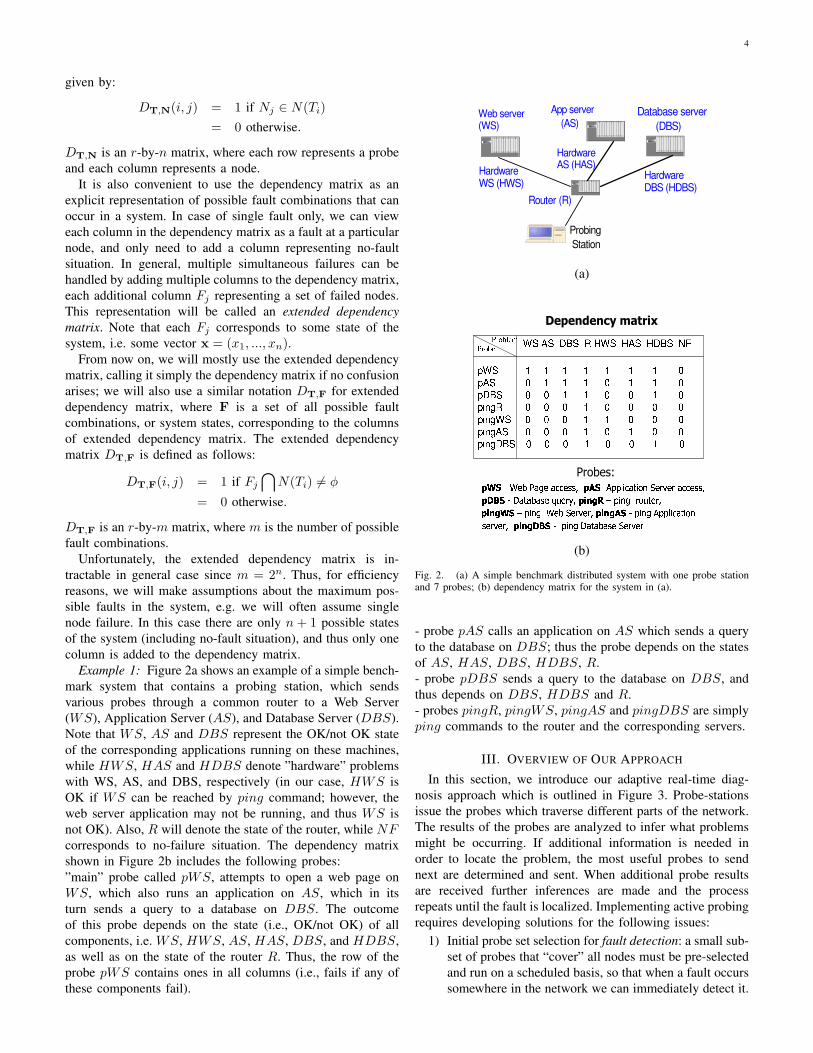
It is useful to introduce the notion of a dependency matrixto capture the relationships between system states and probes.Given any set of nodes N = {N1, N2, ..., Nn} and probes,or tests T = {T1, T2, ..., Tr}, the dependency matrix DT,N is

4

given by:

DT,N(i, j) = 1 if Nj ∈ N(Ti)= 0 otherwise.

DT,N is an r-by-n matrix, where each row represents a probeand each column represents a node.

It is also convenient to use the dependency matrix as anexplicit representation of possible fault combinations that canoccur in a system. In case of single fault only, we can vieweach column in the dependency matrix as a fault at a particularnode, and only need to add a column representing no-faultsituation. In general, multiple simultaneous failures can behandled by adding multiple columns to the dependency matrix,each additional column Fj representing a set of failed nodes.This representation will be called an extended dependencymatrix. Note that each Fj corresponds to some state of thesystem, i.e. some vector x = (x1, ..., xn).

From now on, we will mostly use the extended dependencymatrix, calling it simply the dependency matrix if no confusionarises; we will also use a similar notation DT,F for extendeddependency matrix, where F is a set of all possible faultcombinations, or system states, corresponding to the columnsof extended dependency matrix. The extended dependencymatrix DT,F is defined as follows:

DT,F(i, j) = 1 if Fj

⋂N(Ti) 6= φ

= 0 otherwise.

DT,F is an r-by-m matrix, where m is the number of possiblefault combinations.

Unfortunately, the extended dependency matrix is in-tractable in general case since m = 2n. Thus, for efficiencyreasons, we will make assumptions about the maximum pos-sible faults in the system, e.g. we will often assume singlenode failure. In this case there are only n + 1 possible statesof the system (including no-fault situation), and thus only onecolumn is added to the dependency matrix.

Example 1: Figure 2a shows an example of a simple bench-mark system that contains a probing station, which sendsvarious probes through a common router to a Web Server(WS), Application Server (AS), and Database Server (DBS).Note that WS, AS and DBS represent the OK/not OK stateof the corresponding applications running on these machines,while HWS, HAS and HDBS denote ”hardware” problemswith WS, AS, and DBS, respectively (in our case, HWS isOK if WS can be reached by ping command; however, theweb server application may not be running, and thus WS isnot OK). Also, R will denote the state of the router, while NFcorresponds to no-failure situation. The dependency matrixshown in Figure 2b includes the following probes:”main” probe called pWS, attempts to open a web page onWS, which also runs an application on AS, which in itsturn sends a query to a database on DBS. The outcomeof this probe depends on the state (i.e., OK/not OK) of allcomponents, i.e. WS, HWS, AS, HAS, DBS, and HDBS,as well as on the state of the router R. Thus, the row of theprobe pWS contains ones in all columns (i.e., fails if any ofthese components fail).

(a)

(b)

Fig. 2. (a) A simple benchmark distributed system with one probe stationand 7 probes; (b) dependency matrix for the system in (a).

- probe pAS calls an application on AS which sends a queryto the database on DBS; thus the probe depends on the statesof AS, HAS, DBS, HDBS, R.- probe pDBS sends a query to the database on DBS, andthus depends on DBS, HDBS and R.- probes pingR, pingWS, pingAS and pingDBS are simplyping commands to the router and the corresponding servers.

III. OVERVIEW OF OUR APPROACH

In this section, we introduce our adaptive real-time diag-nosis approach which is outlined in Figure 3. Probe-stationsissue the probes which traverse different parts of the network.The results of the probes are analyzed to infer what problemsmight be occurring. If additional information is needed inorder to locate the problem, the most useful probes to sendnext are determined and sent. When additional probe resultsare received further inferences are made and the processrepeats until the fault is localized. Implementing active probingrequires developing solutions for the following issues:

1) Initial probe set selection for fault detection: a small sub-set of probes that “cover” all nodes must be pre-selectedand run on a scheduled basis, so that when a fault occurssomewhere in the network we can immediately detect it.

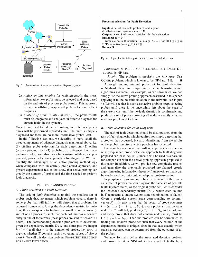
5

Fig. 3. An overview of adaptive real-time diagnosis system.

2) Active, on-line probing for fault diagnosis: the most-informative next probe must be selected and sent, basedon the analysis of previous probe results. This approachextends an off-line, pre-planned probe selection for faultdiagnosis.

3) Analysis of probe results (inference): the probe resultsmust be integrated and analyzed in order to diagnose thecurrent faults in the systems.

Once a fault is detected, active probing and inference proce-dures will be performed repeatedly until the fault is uniquelydiagnosed (or there are no more informative probes left).

In the following sections, we describe in more detail thethree components of adaptive diagnosis mentioned above, i.e.(1) off-line probe selection for fault detection, (2) online(active) probing, and (3) probabilistic inference. For com-pleteness sake, we also describe existing off-line, or pre-planned, probe selection approaches for diagnosis. We thenquantify the advantages of an active probing methodologywhen compared with an entirely pre-planned approach, andpresent experimental results that show that active probing cangreatly the number of probes and the time needed to performfault diagnosis.

IV. PRE-PLANNED PROBING

A. Probe Selection for Fault Detection

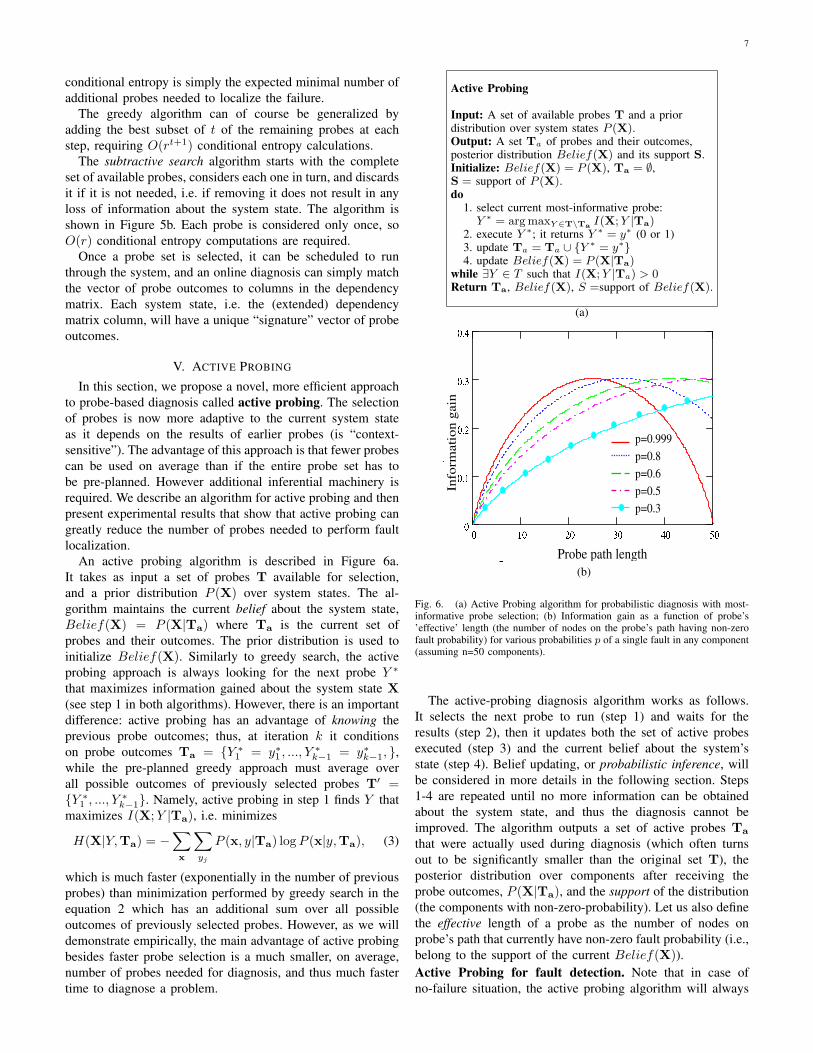
The task of fault detection is to find the smallest set ofprobes such that, no matter which problem occurs, there issome probe that will fail; i.e. will detect that a problem hasoccurred somewhere. Using the dependency matrix formula-tion, this corresponds to finding the smallest set of rows (asubset of all probes T ) such that each column has a nonzeroentry in one of these rows (these probes are said to ”cover” allnodes). The corresponding decision problem is to determine,given the dependency matrix DT,N and some positive integerk ≤ r (recall that r is the number of probes, i.e. rows inDT,N), whether T contains such a covering subset of size atmost k. We call this decision problem PROBE SET SELECTIONFOR FAULT DETECTION.

Probe-set selection for Fault Detection

Input: A set of available probes T and a priordistribution over system states P (X).Output: A set S of probes sufficient for fault detection.Initialize: S = ∅.1. Simulate no-fault situation, i.e. assign Xi = 0 for all 1 ≤ i ≤ n.2. Ta = ActiveProbing(T,P (X)).Return S

Fig. 4. Algorithm for initial probe set selection for fault detection.

Proposition 1: PROBE SET SELECTION FOR FAULT DE-TECTION is NP-hard.

Proof: The problem is precisely the MINIMUM SETCOVER problem, which is known to be NP-hard [11].

Although finding minimal probe set for fault detectionis NP-hard, there are simple and efficient heuristic searchalgorithms available. For example, as we show later, we cansimply use the active probing approach described in this paper,applying it to the no-fault situation in the network (see Figure4). We will see that in such case active probing keeps selectingprobes until there is no uncertainty left about the state ofthe system (i.e. until the no-fault situation is confirmed), andproduces a set of probes covering all nodes – exactly what weneed for problem detection.

B. Probe Selection for Fault Diagnosis

The task of fault detection should be distinguished from thetask of fault diagnosis, which requires not simply detecting thata problem has occurred, but also identifying, from the resultsof the probes, precisely which problem has occurred.

For completeness sake, we will now provide an overviewof a pre-planned probe selection approach to fault diagnosisproposed earlier in [9], [10], since it will be used as a baselinefor comparison with the active probing approach proposed inthis paper. In addition, we will provide new complexity results,and generalize the previously proposed pre-planned greedyalgorithm using information-theoretic framework, so that it canbe easily modified into online, adaptive probe-selection.

In pre-planned probing, our objective is to select the small-est subset of probes that can diagnose the same set of possiblefaults (system states) as the original probe set. Let us considerthe (extended dependency matrix DT,F where each columnin F represents a unique system state (combination of faults).Given a particular system state corresponding to column-vector Fj , it is easy to see that the vector of probe outcomest = (t1, ..., tr) = (D1j , ..., Drj): every probe Ti that containsnodes in Fj will fail, producing Ti = 1 = Dij in the column,and every probe that does not contain nodes in Fj must beOK (Ti = 0 = Dij). Then the problem can be formulated asfinding the smallest probe set such that every column of thedependency matrix is unique, since in that case exactly whichstate has occurred can be determined from the outcomes of allthe probes.

We now formally define the associated decision problemand prove that it is NP-hard. Given a set of faults F, a

6

set of probes T, and a positive integer k ≤ r, we want todetermine whether T contains a subset T′ of size at most ksuch that for every pair of distinct faults f1, f2 ∈ F , thereis a probe T ∈ T′ that intersects exactly one of f1 and f2

(thus T distinguishes between f1 and f2); or equivalently T′ issuch that the columns of the dependency matrix DT′,F are allunique. We call this decision problem PROBE SET SELECTIONFOR FAULT DIAGNOSIS.

Proposition 2: PROBE SET SELECTION FOR FAULT DIAG-NOSIS is NP-hard.

Proof: PROBE SET SELECTION FOR FAULT DIAG-NOSIS can be shown to be NP-hard via a reduction from3-DIMENSIONAL MATCHING. This problem (see [12]) ishowever not very well-known, so it is instructive to reducePROBE SET SELECTION FOR FAULT DIAGNOSIS from PROBESET SELECTION FOR FAULT DETECTION. Intuitively, FAULTLOCALIZATION is a harder problem than FAULT DETECTION.However, because for any given instance the optimal solutionsof these two problems can be very different, the proof is notstraight-forward; the details can be found in the Appendix A.

Although the tasks of finding the smallest probe sets forfault diagnosis is NP-hard, there exist efficient polynomial-time approximation algorithms that perform well in practice.We now present an overview of two such algorithms – greedysearch and subtractive search [9], [10]. We reformulate andgeneralize the greedy search algorithm proposed in [9], [10]using an information-theoretic framework.

Greedy search starts with the empty set and adds at eachstep the “best” of the remaining probes. The “best” probe isthe one which maximizes the information gained about thesystem state, in the sense defined precisely below. Subtrac-tive search starts with the complete set of available probes,considers each one in turn, and discards it if it is not needed.Neither algorithm is optimal in general - experimental resultscomparing their performance with the true minimum probe setsize are given in Section VIII-B.1.

The greedy search approach chooses the next probe bymaximizing the information gained about the system state X,given the previous probes. Formally, let us assume some priorprobability distribution P (X) over possible system states. Weare looking for a probe

Y ∗ = arg maxY ∈T\T′

I(X; Y |T′), (1)

where I(X; Y |T′) is the conditional mutual information of Xand probe Y , given the previously selected probes T′. SinceI(X; Y |T′) = H(X|T′) − H(X|Y,T′), where H(X|Y ) isthe conditional entropy of X given Y (see [13]), the most-informative test Y ∗ minimizes the conditional entropy of X,i.e. the amount of uncertainty about the system state.

The algorithm is shown in Figure 5a. If the initial set ofavailable probes T is of size r, O(r2) conditional entropycalculations are required, since at each step the informationgain obtained by each of the remaining probes must becomputed. Note that

H(X|Y,T) = −∑x

∑yj

∑t

P (x, y, t) log P (x|y, t) (2)

Probe-Set Selection: Greedy Search

Input: A set of available probes T and a priordistribution over system states P (X).Output: A subset T′ ⊆ T of probes.Initialize: T′ = ∅do1. select most-informative next probe:

Y ∗ = arg maxY ∈T\T′ I(X; Y |T′)2. update probe set: T′ = T′ ∪ {Y }

while ∃Y ∈ T\T′ such that I(X; Y |T′) > 0Return T ′.

(a)

Probe-Set Selection: Subtractive Search

Input: A set of available probes T and a priordistribution over system states P (X).Output: A subset T′ ⊆ T of probes.Initialize: T′ = T = {T1, T2, ..., Tr}.for i = 1 to r

remove probe if it is not needed, i.e.if I(X; pi|T′\{Ti}) = 0,then T′ = T′\{Ti}

Return T′.

(b)

Fig. 5. (a) Greedy Search for Probe-Set Selection. (b) Subtractive Searchfor Probe-Set Selection.

so computing the information gain can be quite costly inthe general case, as it requires summation over all non-zero-probability states and outcomes of the current probe set andthe next probe.

The version of greedy search proposed in [9], [10] used thesimplifying assumptions of only one component failing at atime, thus yielding only n+1 system states (including the caseof no failure). Also, all states were assumed to have equal priorprobabilities. These assumptions considerably simplified thecomputation. Let us consider an extended dependency matrixof size r × (n + 1). A probe set cannot distinguish betweensystem states whose columns in the dependency matrix areidentical. Since this is an equivalence relation between states(columns), it induces a decomposition of the states into anexhaustive collection of disjoint subsets, and it is easy to showthat:

H(X|Y,T) =k∑

i=1

ni

mlog ni

where m = n + 1 is the total number of states and ni

is the number of states (columns) in the i’th subset of thedecomposition induced by T.

This expression has a natural interpretation. Since thereare ni states in the i’th subset and each probe has twopossible outcomes, at least log ni additional probes are neededto further decompose the i’th subset into singletons, therebyenabling any single node failure to be diagnosed. Since thetrue failure lies in the i’th subset with probability ni/m, the

7

conditional entropy is simply the expected minimal number ofadditional probes needed to localize the failure.

The greedy algorithm can of course be generalized byadding the best subset of t of the remaining probes at eachstep, requiring O(rt+1) conditional entropy calculations.

The subtractive search algorithm starts with the completeset of available probes, considers each one in turn, and discardsit if it is not needed, i.e. if removing it does not result in anyloss of information about the system state. The algorithm isshown in Figure 5b. Each probe is considered only once, soO(r) conditional entropy computations are required.

Once a probe set is selected, it can be scheduled to runthrough the system, and an online diagnosis can simply matchthe vector of probe outcomes to columns in the dependencymatrix. Each system state, i.e. the (extended) dependencymatrix column, will have a unique “signature” vector of probeoutcomes.

V. ACTIVE PROBING

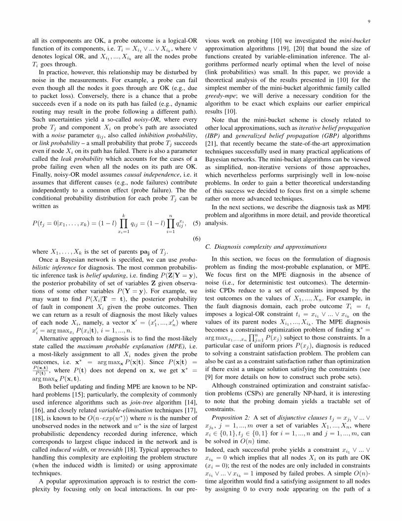
In this section, we propose a novel, more efficient approachto probe-based diagnosis called active probing. The selectionof probes is now more adaptive to the current system stateas it depends on the results of earlier probes (is “context-sensitive”). The advantage of this approach is that fewer probescan be used on average than if the entire probe set has tobe pre-planned. However additional inferential machinery isrequired. We describe an algorithm for active probing and thenpresent experimental results that show that active probing cangreatly reduce the number of probes needed to perform faultlocalization.

An active probing algorithm is described in Figure 6a.It takes as input a set of probes T available for selection,and a prior distribution P (X) over system states. The al-gorithm maintains the current belief about the system state,Belief(X) = P (X|Ta) where Ta is the current set ofprobes and their outcomes. The prior distribution is used toinitialize Belief(X). Similarly to greedy search, the activeprobing approach is always looking for the next probe Y ∗

that maximizes information gained about the system state X(see step 1 in both algorithms). However, there is an importantdifference: active probing has an advantage of knowing theprevious probe outcomes; thus, at iteration k it conditionson probe outcomes Ta = {Y ∗

1 = y∗1 , ..., Y ∗k−1 = y∗k−1, },

while the pre-planned greedy approach must average overall possible outcomes of previously selected probes T′ ={Y ∗

1 , ..., Y ∗k−1}. Namely, active probing in step 1 finds Y that

maximizes I(X; Y |Ta), i.e. minimizes

H(X|Y,Ta) = −∑x

∑yj

P (x, y|Ta) log P (x|y,Ta), (3)

which is much faster (exponentially in the number of previousprobes) than minimization performed by greedy search in theequation 2 which has an additional sum over all possibleoutcomes of previously selected probes. However, as we willdemonstrate empirically, the main advantage of active probingbesides faster probe selection is a much smaller, on average,number of probes needed for diagnosis, and thus much fastertime to diagnose a problem.

Active Probing

Input: A set of available probes T and a priordistribution over system states P (X).Output: A set Ta of probes and their outcomes,posterior distribution Belief(X) and its support S.Initialize: Belief(X) = P (X), Ta = ∅,S = support of P (X).do

1. select current most-informative probe:Y ∗ = arg maxY ∈T\Ta I(X; Y |Ta)

2. execute Y ∗; it returns Y ∗ = y∗ (0 or 1)3. update Ta = Ta ∪ {Y ∗ = y∗}4. update Belief(X) = P (X|Ta)

while ∃Y ∈ T such that I(X; Y |Ta) > 0Return Ta, Belief(X), S =support of Belief(X).

(a)

(b)

Fig. 6. (a) Active Probing algorithm for probabilistic diagnosis with most-informative probe selection; (b) Information gain as a function of probe’s’effective’ length (the number of nodes on the probe’s path having non-zerofault probability) for various probabilities p of a single fault in any component(assuming n=50 components).

The active-probing diagnosis algorithm works as follows.It selects the next probe to run (step 1) and waits for theresults (step 2), then it updates both the set of active probesexecuted (step 3) and the current belief about the system’sstate (step 4). Belief updating, or probabilistic inference, willbe considered in more details in the following section. Steps1-4 are repeated until no more information can be obtainedabout the system state, and thus the diagnosis cannot beimproved. The algorithm outputs a set of active probes Ta

that were actually used during diagnosis (which often turnsout to be significantly smaller than the original set T), theposterior distribution over components after receiving theprobe outcomes, P (X|Ta), and the support of the distribution(the components with non-zero-probability). Let us also definethe effective length of a probe as the number of nodes onprobe’s path that currently have non-zero fault probability (i.e.,belong to the support of the current Belief(X)).Active Probing for fault detection. Note that in case ofno-failure situation, the active probing algorithm will always

8

produce a set of probes that cover all nodes (assuming theinitial probe set allows to cover all nodes). Indeed, its stoppingcondition implies there is no probe that can have a non-zeroinformation about the system state, I(X;Y |Ta). It is easy tosee that while there is at least a single node not covered by aprobe, the system state is still uncertain, and this uncertaintycan be decreased by running an additional probe that goesthrough this node. Once all nodes are covered, the conditionalentropy of the system I(X; Ta) becomes zero, and the activeprobing stops. Thus, simulating no-fault situation and runningactive probing will produce a set of probes sufficient forproblem detection.

VI. ANALYSIS OF PROBE RESULTS: PROBABILISTICINFERENCE

A. Diagnosis under Simplifying Assumptions

In our current implementation of active probing, we madesimplifying assumptions of having no more than s simultane-ous faults (usually, setting s = 1 as having simultaneous faultswas highly unlikely in systems we considered), which yieldsmore than 2s system states. For small s the explicit state spacerepresentation is relatively small (e.g., it is linear in the numberof nodes for single-fault assumption), and thus we can easilyupdate the joint distribution P (X) over all possible states ofthe system. However, for generic multi-fault diagnosis, moreefficient algorithms, including approximations, are needed. Anextension to generic multi-fault diagnosis will be consideredin the subsequent sections.

Besides single-fault assumption, we also used a simpleexpressions for priors, assuming 1− p probability of no-faultsituation, and uniformly distributed probability mass p amongthe remaining states (possible single component failures),which gave us P (Xi = 1, Xj = 0∀j 6= i) = p/n. In thiscase the information gain of a probe can be computed quiteefficiently (see Appendix B for details):

I(X;T ) = I(p, n, k) = −(1− p) log(1− p)− p logp

n

−kp

nlog k + (1− p) log

1− p

1− k pn

+ (n− k)p

nlog

p

n− pk. (4)

Figure 6b plots the information gain of a probe as a functionof its effective length k, for n = 50 nodes and for variousfault priors. It is more beneficial to send probes with largereffective length if the probability of fault p is small. However,once a fault is detected (p = 1), the most informative probe(i.e. a probe attaining the maximum information gain) is onewhose effective length is closest to half the number of nodesthat are possibly faulty.

In the single-fault case, if the complete set of availableprobes is sufficient for diagnosis, the support set S output bythe algorithm will contain the unique component that is down.In general, the active probing algorithm can be applied toany multiple-fault situation; however, its complexity increaseswith an increasing number of simultaneous faults and dependson the efficiency of representing the joint probability P (X)and the efficiency of probabilistic inference and information-gain computation required for active probe selection. It mayalso become impossible to update the joint distribution, i.e.

Fig. 7. A mapping from dependency matrix to a Bayesian network.

Belief(X). Instead, we will have to modify the line 4in the Active Probing algorithm: given the previous probeobservations, instead of updating joint belief, we may need toupdate the beliefs of individual nodes and return their most-likely values, or to find directly the most-likely state of thesystem as a 0/1 assignment to all nodes. The problem of multi-fault diagnosis is considered in the following section.

B. Multi-Fault Diagnosis using Bayesian Networks

Active probing algorithm described in the previous sectionmust use some representation of the joint probability distri-bution P (X) and a belief updating method. While in caseof small number of possible states (e.g., n + 1 states undersingle-fault assumption) the joint distribution P (X) can bespecified explicitly, this representation becomes intractable inthe general case of multiple faults. In this case, fault diagnosisalgorithms can benefit from using a probabilistic graphicalmodel such as Bayesian network [14], which describes theprobability distribution over the system states in a compactform. For example, the (original) dependency matrix canbe easily mapped to a two-layer Bayesian network whereeach component Xi corresponds to an upper-level variablerepresenting the state of node Ni, each probes Tj correspondsto a lower-layer variable, and each subset N(Tj) correspondsto the set of parents of variable Tj (i.e., nodes pointing toTj) in the Bayesian network, also denoted paj (see Figure 7).Recall that Xi = 1 and Tj = 1 if node Ni and probe Tj arefaulty, respectively; and Xi = 0 and Tj = 0 otherwise. Thenthe joint probability distribution can be written as

P (x, t) =n∏

i=1

P (xi)m∏

j=1

P (tj |paj),

assuming that the state variables Xi’s are marginally in-dependent, and that each probe outcome depends only onthe components tested by this probe. P (xi) specifies theprior probabilities of the system states, while the conditionalprobabilities distributions (CPDs) P (tj |paj) describe the de-pendency of probe outcomes on the components tested. Inthe absence of noise in the probe outcomes, all CPDs aredeterministic functions. Since a probe succeeds if and only if

9

all its components are OK, a probe outcome is a logical-ORfunction of its components, i.e. Ti = Xi1 ∨ ...∨Xik

, where ∨denotes logical OR, and Xi1 , ..., Xik

are all the nodes probeTi goes through.

In practice, however, this relationship may be disturbed bynoise in the measurements. For example, a probe can faileven though all the nodes it goes through are OK (e.g., dueto packet loss). Conversely, there is a chance that a probesucceeds even if a node on its path has failed (e.g., dynamicrouting may result in the probe following a different path).Such uncertainties yield a so-called noisy-OR, where everyprobe Tj and component Xi on probe’s path are associatedwith a noise parameter qij , also called inhibition probability,or link probability – a small probability that probe Tj succeedseven if node Xi on its path has failed. There is also a parametercalled the leak probability which accounts for the cases of aprobe failing even when all the nodes on its path are OK.Finally, noisy-OR model assumes causal independence, i.e. itassumes that different causes (e.g., node failures) contributeindependently to a common effect (probe failure). The theconditional probability distribution for each probe Tj can bewritten as

P (tj = 0|x1, . . . , xk) = (1− l)k∏

xi=1

qij = (1− l)n∏

i=1

qxiij , (5)

(6)

where X1, . . . , Xk is the set of parents paj of Tj .Once a Bayesian network is specified, we can use proba-

bilistic inference for diagnosis. The most common probabilis-tic inference task is belief updating, i.e. finding P (Z|Y = y),the posterior probability of set of variables Z given observa-tions of some other variables P (Y = y). For example, wemay want to find P (Xi|T = t), the posterior probabilityof fault in component Xi given the probe outcomes. Thenwe can return as a result of diagnosis the most likely valuesof each node Xi, namely, a vector x′ = (x′1, ..., x

′n) where

x′i = arg maxxi P (xi|t), i = 1, ..., n.Alternative approach to diagnosis is to find the most-likely

state called the maximum probable explanation (MPE), i.e.a most-likely assignment to all Xi nodes given the probeoutcomes, i.e. x∗ = arg maxx P (x|t). Since P (x|t) =P (x,t)P (t) , where P (t) does not depend on x, we get x∗ =

arg maxx P (x, t).Both belief updating and finding MPE are known to be NP-

hard problems [15]; particularly, the complexity of commonlyused inference algorithms such as join-tree algorithm [14],[16], and closely related variable-elimination techniques [17],[18], is known to be O(n ·exp(w∗)) where n is the number ofunobserved nodes in the network and w∗ is the size of largestprobabilistic dependency recorded during inference, whichcorresponds to largest clique induced in the network and iscalled induced width, or treewidth [18]. Typical approaches tohandling this complexity are exploiting the problem structure(when the induced width is limited) or using approximatetechniques.

A popular approximation approach is to restrict the com-plexity by focusing only on local interactions. In our pre-

vious work on probing [10] we investigated the mini-bucketapproximation algorithms [19], [20] that bound the size offunctions created by variable-elimination inference. The al-gorithms performed nearly optimal when the level of noise(link probabilities) was small. In this paper, we provide atheoretical analysis of the results presented in [10] for thesimplest member of the mini-bucket algorithmic family calledgreedy-mpe; we will derive a necessary condition for thealgorithm to be exact which explains our earlier empiricalresults [10].

Note that the mini-bucket scheme is closely related toother local approximations, such as iterative belief propagation(IBP) and generalized belief propagation (GBP) algorithms[21], that recently became the state-of-the-art approximationtechniques successfully used in many practical applications ofBayesian networks. The mini-bucket algorithms can be viewedas simplified, non-iterative versions of those approaches,which nevertheless performs surprisingly well in low-noiseproblems. In order to gain a better theoretical understandingof this success we decided to focus first on a simple schemerather on more advanced techniques.

In the next sections, we describe the diagnosis task as MPEproblem and algorithms in more detail, and provide theoreticalanalysis.

C. Diagnosis complexity and approximations

In this section, we focus on the formulation of diagnosisproblem as finding the most-probable explanation, or MPE.We focus first on the MPE diagnosis in the absence ofnoise (i.e., for deterministic test outcomes). The determin-istic CPDs reduce to a set of constraints imposed by thetest outcomes on the values of X1, ..., Xn. For example, inthe fault diagnosis domain, each probe outcome Ti = tiimposes a logical-OR constraint ti = xi1 ∨ ... ∨ xik

on thevalues of its parent nodes Xi1 , ..., Xik

. The MPE diagnosisbecomes a constrained optimization problem of finding x∗ =arg maxx1,...,xn

∏nj=1 P (xj) subject to those constraints. In a

particular case of uniform priors P (xj), diagnosis is reducedto solving a constraint satisfaction problem. The problem canalso be cast as a constraint satisfaction rather than optimizationif there exist a unique solution satisfying the constraints (see[9] for more details on how to construct such probe sets).

Although constrained optimization and constraint satisfac-tion problems (CSPs) are generally NP-hard, it is interestingto note that the probing domain yields a tractable set ofconstraints.

Proposition 2: A set of disjunctive clauses tj = xj1 ∨ ...∨xjk

, j = 1, ..., m over a set of variables X1, ..., Xn, wherexi ∈ {0, 1}, tj ∈ {0, 1} for i = 1, ..., n and j = 1, ..., m, canbe solved in O(n) time.Indeed, each successful probe yields a constraint xi1 ∨ ... ∨xik

= 0 which implies that all nodes Xi on its path are OK(xi = 0); the rest of the nodes are only included in constraintsxi1 ∨ ...∨ xik

= 1 imposed by failed probes. A simple O(n)-time algorithm would find a satisfying assignment to all nodesby assigning 0 to every node appearing on the path of a

10

successful probe, and 1 to the rest of nodes2.In the presence of noise, the MPE diagnosis task can be

written as finding x∗ = arg maxx1 . . . maxxn

∏i P (xi|pai) =

= arg maxx1

F1(x1) . . . maxxn

Fn(xn, Sn), (7)

where each Fi(xi,Si) =∏

xkP(xk|pa(xk)) is the product

of all probabilistic components involving Xi and a subset oflower-index variables Si ⊆ {X1, ...,Xi−1}, but not involvingany Xj for j > i. The set of all such components is also calledthe bucket of Xi [18]. An exact algorithm for finding MPEsolution, called elim-mpe [18], uses variable-elimination (alsocalled bucket-elimination) as a preprocessing: it computes theproduct of functions in the bucket of each variable Xi, fromi = n to i = 1 (i.e., from right to left in the equation 7),maximizes it over Xi, and propagates the resulting functionf(·) to the bucket of its highest-order variable. Once variable-elimination is completed, the algorithm finds an optimal so-lution by a backtrack-free greedy procedure that, going fromi = 1 to i = n (i.e., in the opposite direction to elimination),assigns Xi = arg maxxi

Fi(xi,Si = si) where Si = si isthe current assignment to Si. It is shown that elim-mpe isguaranteed to find an optimal solution and that the complexityof the variable-elimination step is O(n · exp(w∗)) where w∗,called the induced width, is the largest number of argumentsamong the functions (old and newly recorded) in all buckets[18]. For the probing domain, it is easy to show that w∗ ≥ kwhere k is the maximum number parents of a probe node, andw∗ = n in the worst case.

Since the exact MPE diagnosis is intractable for large-scale networks, we focused on local approximation techniques.Particularly, we used a simple (O(n) time) backtrack-freegreedy algorithm, called here greedy-mpe, which performsno variable-elimination preprocessing, and the simplest andfastest member of the mini-bucket approximation family, algo-rithm approx-mpe(1) [19], [20], that performs a very limitedpreprocessing similar to relational arc-consistency [20] inconstraint networks.

The greedy algorithm greedy-mpe does no preprocessing(except for replacing observed variables with their values inall related function prior to algorithm’s execution). It computesa suboptimal solution

x′ = (arg maxx1

F1(x1), . . . , ..., arg maxxn

Fn(xn, Sn = sn)),(8)

where Si = si, as before, denotes the current assignmentto the variables in Sj computed during the previous i − 1maximization steps.

Generally, the mini-bucket algorithms approx-mpe(i) per-form a limited level of variable-elimination, similar to en-forcing directional i-consistency, prior to the greedy assign-ment. The preprocessing allows to find an upper bound Uon M = maxx P (x, t), where t is the evidence (clearly,MPE = M/P (t)), while the probability L = P (x′, e)of their suboptimal solution provides an lower bound on

2Note that this is equivalent to applying unit propagation to a Horn theory– a propositional theory that contains a collection of disjunctive clauses, ordisjuncts, where each disjunct includes no more than one positive literal.

M . Generally, L increases with the level of preprocessingcontrolled by i, thus allowing a flexible accuracy vs. efficiencytrade-off. The algorithm returns the suboptimal solution x′ andthe upper and lower bounds, U and L, on M ; ratio U/L is ameasure of the approximation error.

In [10], the algorithms greedy-mpe and approx-mpe(1) weretested on the networks constructed in a way that guarantees theunique diagnosis in the absence of noise. Particularly, besidesm tests each having r randomly selected parents, we alsogenerated n direct tests T̂i, i = 1, ..., n, each having exactlyone parent node Xi. It is easy to see that, for such networks,both greedy-mpe and approx-mpe(1) find an exact diagnosisin the absence of noise: approx-mpe(1) reduces to the unit-propagation, an equivalent of relational-arc-consistency, whilegreedy-mpe, applied along a topological order of variablesin the network’s directed acyclic graph (DAG)3, immediatelyfinds the correct assignment which simply equals the outcomesof the direct tests.

We then added noise in a form of non-zero link probabilityq (assumed to be equal for all nodes), and zero leak proba-bility. The Figure 8 summarizes the results for 50 randomlygenerated networks with n = 15 unobserved nodes (havinguniform fault priors p = P (xi = 0) = 0.5), n = 15 directprobes, one for each node, and m = 15 noisy-OR probes, eachwith r = 4 randomly selected parents among the unobservednodes, zero leak l = 0 probability. The link probability (noiselevel) q varied from 0.01 to 0.64, taking 15 different values;the results are shown for all noise levels together. For eachnetwork, 100 instances of evidence (probe outcomes) weregenerated by Monte-Carlo simulation of x and t accordingto their conditional distributions. Thus, we get 50x100=5000samples for each value of noise q.

As demonstrated in Figure 8, the approximation accuracyof greedy-mpe, measured as L/M where L = P (x′, t) andM = P (x∗, t), clearly increases with increasing value M , andtherefore with the probability of the exact diagnosis, whichalso depends on the ”diagnostic ability” of a probe set (forsame probe set size, a better probe set yields a higher MPEdiagnosis, and therefore, a better approximation quality). Thereis an interesting threshold phenomenon, observed both forgreedy-mpe and for approx-mpe(1) solutions (the results forapprox-mpe(1) are omitted due to space restrictions), and forvarious problem sizes n: the suboptimal solution x′ found byalgorithm greedy-mpe suddenly becomes (almost always) anexact solution x∗ (i.e., L/M = 1, where L = P (x′, t) andM = P (x∗, t)) when M > θ where θ is some thresholdvalue. For n = 15, the threshold is observed between 2e − 6and 3e− 6. A theoretical analysis in the next section yields aquite accurate prediction of θ ≈ 2.46e− 6.

1) Theoretical analysis: noise and approximation accuracy:We now provide a theoretical explanation for threshold be-havior of approximation error reported in [10], at least for thesimplest approximation algorithm greedy-mpe.

Let BN = (G,P ) be a Bayesian network, where T = tis evidence, i.e. a value assignment t to a subset of variables

3A topological (or ancestral) ordering of a DAG is an ordering where achild node never appears before its parent.

11

0 0.246 0.5 1 1.5 2 2.5 3

x 10−5

0

0.1

0.2

0.3

0.4

0.5

0.6

0.7

0.8

0.9

1

MPE

App

rox.

qua

lity:

L/M

15 nodes, 15 tests, 4 parents

Fig. 8. The accuracy of the solution x′ found by algorithm greedy-mpe,measured by L/M , where L = P (x′, t) and M = P (x∗, t), versus M . Theresults obtained for approx-mpe(1) were quite similar to those for greedy-mpe.

T ⊂ X. We will also make an important assumption thatthe all observed variables are replaced by their values in allCPD functions. Also, recall that Fi(xi, si) is the product offunctions in the bucket of Xi along the ordering o, given theassignment si of some variables in the previous buckets. Then

Lemma 3 (greedy-mpe optimality): Given a Bayesian net-work BN = (G,P ), an evidence assignment T = t appliedto all relevant probability functions, and a topological orderingo of unobserved nodes in the graph G, the algorithm greedy-mpe applied along o is guaranteed to find an optimal MPEsolution if P (x′, t) ≥ Fi(xi, s′i) for every i = 1, ..., n and forevery xi 6= x′i, where Si = s′i is a partial assignment alreadyfound by greedy-mpe.

Proof: Clearly, the solution x′ found by greedy-mpeis optimal, i.e. x′ = x∗ = arg maxx P (x, t) if P (x′, t) ≥P (x, t) for every x 6= x′. Since x 6= x′ implies xi 6= x′i forsome i (let us choose the smallest of such i’s), by the con-dition of lemma we get P (x′, t) ≥ Fi(xi, s′i), and, therefore,P (x′, t) ≥ ∏n

j=1 Fj(xj , sj) since each Fj(xj , sj) is a productof probabilities, and therefore, 0 ≥ Fj(xj , sj) ≥ 1. But∏n

j=1 Fj(xj , sj) = P(x, t) by equation 7, which concludesthe proof.

We now discuss some particular classes of Bayesian net-works that satisfy the conditions of lemma 3.

Lemma 4 (nearly-deterministic CPDs, no observations):Given a Bayesian network BN = (G, P ) having no observedvariables, and all conditional (and prior) probabilitiesbeing nearly-deterministic, i.e. satisfying the conditionmaxxi P (xi|pa(Xi)) > 1 − δ, where 0 ≤ δ ≤ 0.5, algorithmgreedy-mpe applied along a topological ordering o of G isguaranteed to find an optimal MPE assignment if (1−δ)n ≥ δ.

Proof: Given a topological ordering and no evidencevariables, the bucket of every node Xi contains a singlefunction P (xi|pa(Xi)). Thus, the greedy solution x′ yieldsP (x′) =

∏ni=1 maxxi P (xi|pa(Xi)) = (1 − δ)n, while any

other x has the probability P (x) =∏n

i=1 P (xi|pa(Xi)) <δ since for the very first i such that xi 6= x′i we getP (xi|pa(Xi)) < δ and this value can only decrease when

multiplied by other probabilities 0 ≤ P (xj |pa(Xj)) ≤ 1.Let us consider a simulation that happened to select

only the most-likely values for T̂i and Ti, i.e. t′i =arg maxti

P (ti|pa(Ti)), which can be viewed as an error-free ”transmission over a noisy channel”. From 6 weget maxti

P (ti|pa(Ti)) ≥ (1 − q); also, for any t′′i 6=arg maxti P (ti|pa(Ti)), P (t′′i |pa(Ti)) < q. It is easy to show(similarly to lemma 3) that algorithm greedy-mpe will findan assignment that produced this most-likely evidence, thusyielding P (x′, t̂, t) =

∏ni=1 P (xi)

∏ni=1 P (t̂i)

∏ni=1 P (ti) >

12n (1−q)n+m. On the other hand, for any other x there existsTj = tj where tj is not the most-likely choice for Tj givenx, and thus P (ti|pa(ti)) < q as can be seen from the noisy-OR definition. Thus, the greedy solution x′ is guaranteed tobe optimal once for any x 6= x′, P (x′, t̂, t) > P (x, t̂, t),i.e. once (1 − q)n+m > q (the constant 1

2n on both sides ofthe inequality was cancelled). Note that simulating an unlikelyevidence yields a low joint probability M = P (x∗, t̂, t) < qfor the optimal diagnosis x∗.

In our experiments, n = m = 15, thus resolving (1−q)30 =q gives a threshold value q ≈ 0.0806, and therefore M =P (x′, t̂, t) = 1

215 (1 − q)30 > 1215 q ≈ 2.46e − 6, which is

surprisingly close to the empirical threshold observed in Figure8 which separates suboptimal from the optimal behavior ofalgorithm greedy-mpe.

VII. EMPIRICAL RESULTS

This section examines the empirical behavior of both pre-planned and active probing. For pre-planned probing theapproximation algorithms find a probe set which is veryclose to the true minimum set size, and can be effectivelyused on large networks where finding the true minimumby exhaustive search is impractical. Active probing greatlyreduces the number of probes needed, although at the expenseof a more complex interactive inferencing system, as describedabove.

A. Simulated Networks

Our initial set of experiments was performed on randomlygenerated networks. Of course, those artificial networks maynot necessarily reflect the realistic topologies, but they stillprovide an initial comparison of active probing to otherapproaches; then, the next section demonstrates active probingon real-life networks.

The artificial networks in our experiments were generated asfollows. For each network size n, we generated twenty randomnetworks with n nodes by randomly connecting each node tofour other nodes. The probe stations are selected randomly.The probes follow the least-cost path from each probe stationto each node.

The states to diagnose are any single node being down orno failure anywhere in the network. Each node has the sameprior probability of failure, and there is no noise in the proberesults. Note that in this case n probes are sufficient, becauseone can always use just one probe-station and probe everysingle node.

12

(a)

(b)

Fig. 9. Active versus pre-planned probing results for randomly generatednetworks: simulation results on (a) small-scale and (b) large-scale networks.

Exhaustive search is performed to find the true mini-mum size probe set. Then linear-time subtractive search andquadratic-time greedy search are used to find probe sets.Active probing algorithm is evaluated as follows. For eachnetwork, we simulate all possible fault scenarios (i.e., a faultat each node, and the no-failure situation), and compute anaverage number of active probes needed for diagnosis in thisnetwork. Finally, for every probing method, we average theresults over all networks of given size and report them inFigure 9.

The results in Figure 9a (small-scale networks) indicate thatthe approximation algorithms for finding the smallest probe setperform well and are much closer to the true minimum set sizethan to the upper bound of n probes and also demonstratethe considerable improvement resulting from active probingwhen compared with pre-planned, or “passive”, probing. InFigure 9b the approximation and active probing algorithmsare extended to larger networks for which finding the trueminimum is impractical. The active probing demonstrates

Fig. 10. Active probing results on several practical problems.

more than 60% improvement over the pre-planned probing.

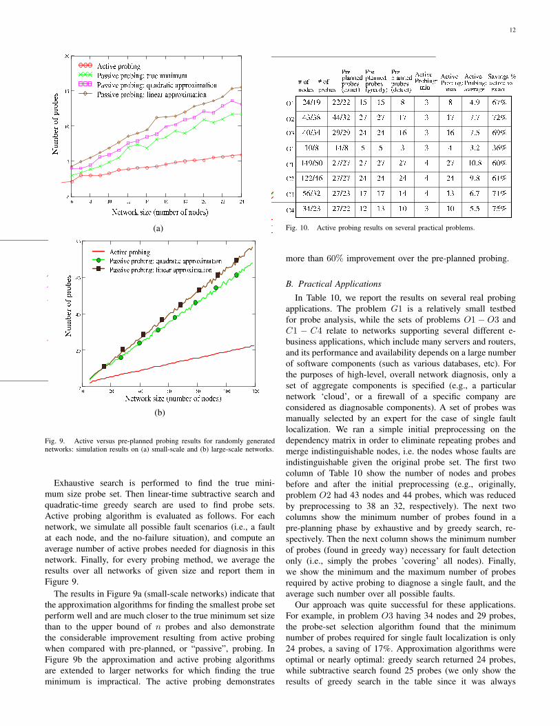
B. Practical Applications

In Table 10, we report the results on several real probingapplications. The problem G1 is a relatively small testbedfor probe analysis, while the sets of problems O1 − O3 andC1 − C4 relate to networks supporting several different e-business applications, which include many servers and routers,and its performance and availability depends on a large numberof software components (such as various databases, etc). Forthe purposes of high-level, overall network diagnosis, only aset of aggregate components is specified (e.g., a particularnetwork ‘cloud’, or a firewall of a specific company areconsidered as diagnosable components). A set of probes wasmanually selected by an expert for the case of single faultlocalization. We ran a simple initial preprocessing on thedependency matrix in order to eliminate repeating probes andmerge indistinguishable nodes, i.e. the nodes whose faults areindistinguishable given the original probe set. The first twocolumn of Table 10 show the number of nodes and probesbefore and after the initial preprocessing (e.g., originally,problem O2 had 43 nodes and 44 probes, which was reducedby preprocessing to 38 an 32, respectively). The next twocolumns show the minimum number of probes found in apre-planning phase by exhaustive and by greedy search, re-spectively. Then the next column shows the minimum numberof probes (found in greedy way) necessary for fault detectiononly (i.e., simply the probes ’covering’ all nodes). Finally,we show the minimum and the maximum number of probesrequired by active probing to diagnose a single fault, and theaverage such number over all possible faults.

Our approach was quite successful for these applications.For example, in problem O3 having 34 nodes and 29 probes,the probe-set selection algorithm found that the minimumnumber of probes required for single fault localization is only24 probes, a saving of 17%. Approximation algorithms wereoptimal or nearly optimal: greedy search returned 24 probes,while subtractive search found 25 probes (we only show theresults of greedy search in the table since it was always

13

superior to subtractive search). Finally, the most impressiveresults were obtained by active probing. The number of probesneeded never exceeded 16 probes; on average, active probingrequired only 7.5 probes, versus 24 probes used by pre-plannedprobing, which yields savings of 69% (and of almost 74% ifthe initial probe set is considered). In most of the cases (exceptfor a small testbed problem G1), active probing was savingfrom 60% to 75% probes if compared to pre-planned probing(and even more if compared to the initial probe set size).

VIII. MODELLING CHANGE IN DYNAMIC SYSTEMS

Many commonly used approaches to diagnosis (includingthe codebook [7] and the active probing described above)assume that the system does not change during the diagnosis.Namely, the probe outcomes are obtained while the system isin a certain state that we wish to recover from the observations.However, this is not the case in highly dynamic systemswhere the failure and repair rates are comparable with averagediagnosis time. In such cases, probes can provide contradictoryinformation: e.g. same probe which failed a couple of minutesago is OK now - does this mean a repair occurred (i.e., thefailure was intermittent) or one of the probe outcome wasincorrect (noisy probe outcomes)? In ”static” approaches, suchinconsistencies are typically treated as noise [7], and may(unnecessarily) increase the diagnostic error.

Another challenge is the presence of multiple safe faultswhich become more likely with the growing size of a dynamicsystem. ”Static” approaches (e.g. codebook) do not track thesequential occurrence of the faults (and repairs), and thus facethe problem of diagnosing simultaneous multiple faults presentin the system. However, general multifault diagnosis prob-lem is known to be computationally hard (e.g., constrained-satisfaction formulation of [22] and probabilistic inferenceproblem in Bayesian networks [1] are both NP-hard; also,handling multiple faults in a system of n components usingcodebook [7] or active probing [3] would require enumerationof up to 2n fault combinations).

Herein, we propose two approaches to handling dynamicsystems. The first one is a general framework of DynamicBayesian Networks (DBNs), that can handle a wide range ofdynamic systems, but suffers from same computational com-plexity problem as the basic Bayesian network framework (i.e.,inference in DBNs is NP-hard). The second one is an efficientlinear-time approximation, called herein sequential multifaultapproach. This approach provides significant computationalsavings over general multifault approaches (such as BNs andDBNs), while at the same improves the accuracy of ”static”approaches (such as codebook and single-fault active probing).The price to pay is the restricting assumptions that failuresand repairs happen only one at a time and with a relativelylow frequency so that the diagnostic engine can process themsequentially. However, there appears to be a wide range ofpractical diagnostic problems satisfying these assumptions,where our approach provides a nice trade-off between accuracyand complexity of diagnosis.

A. Dynamic Bayesian Networks

In order to model situations where the states of systemcomponents change over time, we will first consider generalframework of Dynamic Bayesian Networks (DBNs). DynamicBN model extends static BN model by introducing the notionof time, namely, by adding time slices and specifying transitionprobabilities between these slices: P (Xt|Xt−1), where Xt =(xt

1, ...xtn) is the vector of node states at time slice t. DBNs

use the Markov assumption that the future system state isindependent of its past states given the present state. Of course,a brute-force specification of such probability over binaryvariables requires a table of size O(22n), but the dynamicBayesian network exploits the conditional independencies (justas regular BN) which allow to decompose the transitionprobability into a product of transition probabilities for eachnode at time slice t. As a result, a DBN is defined as a two-slice BN, where the intra-slice dependencies are described by astatic BN, and inter-slice dependencies describe the transitionprobabilities. It is usually assumed that DBN describes astationary stochastic process (i.e. the transition probabilitiesand intra-slice dependencies do not change with time), thusonly two slices are enough to describe the process. Figure 11bshows an example of a dynamic BN that extends a static BNin Figure 11a (describing intra-slice dependencies) by addinginter-slice dependencies encoding transition probabilities. Forexample, the state of node X1 at time t + 1 depends on thestates of nodes X1 and X2 at time t, which is described bya transition probability distribution P (Xt+1

1 |Xt1, X

t2). Node

T tj denotes j-th probe outcome observed at time t; note

that at different time slices, different probes can be observed(sometimes simultaneously, depending on the size of time slicewith respect to probe time window).

(a)

(b)

Fig. 11. (a) A two-layer Bayesian network structure for a set X =(X1, X2, X3) of network elements and a set of probes T = (T1, T2), and(b) its extension to a Dynamic Bayesian Network.

Once a dynamic BN is specified, any standard BayesianNetwork inference algorithm can be applied to the two-slicedynamic BN in order to compute P (Xt|Xt−1, Y t), given theprior distribution P (Xt−1) and the observations Y t at time

14

slice t (where Y ⊆ T is a subset of probes observed at timet). Clearly, this process can be repeated iteratively over time,always producing the joint distribution over the system statesat the current time and the most-likely diagnosis. Although thecomputational complexity of exact inference in DBNs can bequite high, up to O(2n), where n is the number of nodes at atime slice, there are some efficient approximation algorithmsavailable [23], [24].

1) Learning Dynamic Bayesian Networks: In order to applydynamic Bayesian networks to our diagnostic problems wewill need to obtain transition probability parameters, as well asthe probe outcome probabilities (in case of noisy probes). Re-call that we are only given the dependency matrix that definesthe intra-slice structure; the inter-slice structure we assume tobe quite simple: each node fails and repairs independently ofthe others, thus every node state at time t− 1 affects only itsstate at the next time step, and vice versa, every node’s statenow is only affected by its own state on the previous time slice.However, the probability parameters must be learned fromdata, such as sequences of probe observations over severaltime slices.

A standard approach to learning DBNs from sequentialdata is to use Expectation-Maximization (EM) [25] algorithmwhich is a generic technique for learning probabilistic modelswith hidden variables (i.e. variables that are not observed,or missing in the data). The algorithm works iterativelyas follows: it uses some initial parameter assignment tocompute the expected values of certain sufficient statistics(e.g., frequencies in case of maximum-likelihood probabilityestimates) which cannot be computed directly due to missingvalues of certain variables (this is called the E-step); thenthe expected statistics are used instead of ”real” ones (as ifthey were computed from the data without hidden variables)and either a maximum-likelihood approach or, alternatively,MAP - maximum-aposteriory probability approach which usesBayesian priors over the parameters – is applied in order tocompute updated parameters (M-step); the new parametersreplace the ones from the first iteration, and the algorithmcontinues recursively. It is known to converge to a localmaximum in parameter space under quite general assumptions.

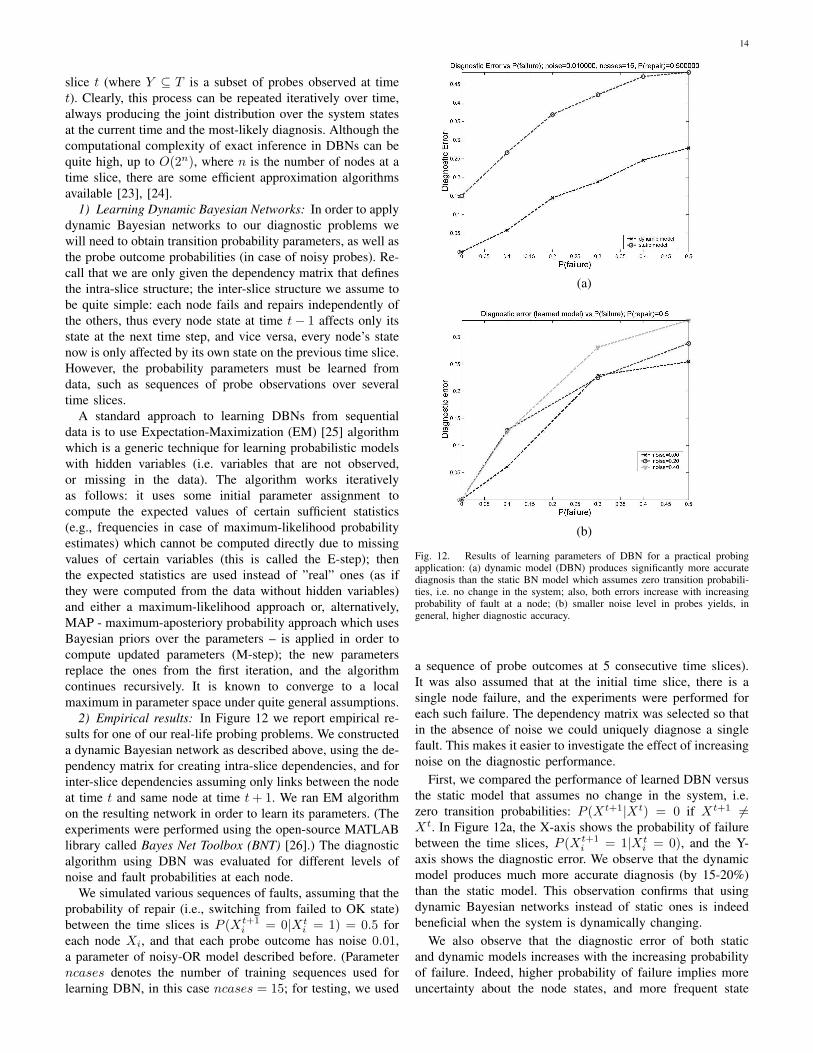
2) Empirical results: In Figure 12 we report empirical re-sults for one of our real-life probing problems. We constructeda dynamic Bayesian network as described above, using the de-pendency matrix for creating intra-slice dependencies, and forinter-slice dependencies assuming only links between the nodeat time t and same node at time t + 1. We ran EM algorithmon the resulting network in order to learn its parameters. (Theexperiments were performed using the open-source MATLABlibrary called Bayes Net Toolbox (BNT) [26].) The diagnosticalgorithm using DBN was evaluated for different levels ofnoise and fault probabilities at each node.

We simulated various sequences of faults, assuming that theprobability of repair (i.e., switching from failed to OK state)between the time slices is P (Xt+1

i = 0|Xti = 1) = 0.5 for

each node Xi, and that each probe outcome has noise 0.01,a parameter of noisy-OR model described before. (Parameterncases denotes the number of training sequences used forlearning DBN, in this case ncases = 15; for testing, we used

(a)

(b)

Fig. 12. Results of learning parameters of DBN for a practical probingapplication: (a) dynamic model (DBN) produces significantly more accuratediagnosis than the static BN model which assumes zero transition probabili-ties, i.e. no change in the system; also, both errors increase with increasingprobability of fault at a node; (b) smaller noise level in probes yields, ingeneral, higher diagnostic accuracy.

a sequence of probe outcomes at 5 consecutive time slices).It was also assumed that at the initial time slice, there is asingle node failure, and the experiments were performed foreach such failure. The dependency matrix was selected so thatin the absence of noise we could uniquely diagnose a singlefault. This makes it easier to investigate the effect of increasingnoise on the diagnostic performance.

First, we compared the performance of learned DBN versusthe static model that assumes no change in the system, i.e.zero transition probabilities: P (Xt+1|Xt) = 0 if Xt+1 6=Xt. In Figure 12a, the X-axis shows the probability of failurebetween the time slices, P (Xt+1

i = 1|Xti = 0), and the Y-

axis shows the diagnostic error. We observe that the dynamicmodel produces much more accurate diagnosis (by 15-20%)than the static model. This observation confirms that usingdynamic Bayesian networks instead of static ones is indeedbeneficial when the system is dynamically changing.

We also observe that the diagnostic error of both staticand dynamic models increases with the increasing probabilityof failure. Indeed, higher probability of failure implies moreuncertainty about the node states, and more frequent state

15

change.Figure 12b also shows how the diagnostic error increases

with the (transitional) probability of failure, now for differentlevels of noise. As expected, we observe that the smallernoise levels generally yield a more accurate diagnosis. Thiscorresponds to our intuition since more deterministic probestend to keep more information about the true states of thenodes they go through; thus, learning uses more informativedata.

B. Sequential Multifault Approach: an Efficient Approxima-tion to DBNs

As we already mentioned above, the problem with DBNsis the computational complexity of inference that can be gen-erally hard (NP-hard). Herein, we propose an approximationto DBNs based on simplifying assumptions regarding thefault occurrence: namely, we assume that failures and repairshappen one at a time, and the time between such events issufficient for diagnostic engine to complete its cycle. Ourapproach can be also viewed as a very simple extension of thesingle-fault active probing algorithm (and it will be describedin detail using the dependency matrix terminology).

Note that some multifault situations can be inherently unrec-ognizable because some components may become ”shielded”by the failures of other components. Particularly, in depen-dency matrix setting, we will define a component X as shieldedby the failure of the component Y if all probes going throughX go through Y as well.Generic Multifault. First, we consider a very simple algo-

rithm for handling multiple faults (called generic multifault)that still assumes no change in the system state during thediagnosis cycle. Given the dependency matrix and the probesoutcomes, the algorithm1. Finds OK nodes: these are all the nodes through which atleast one OK probe passed.2. Finds failed nodes: these are the nodes through which anyfailed probe passed such that all other nodes on its path areOK nodes, as determined in step 1.3. Finds shielded nodes: these are the nodes through whichno probe goes other than those that go through any of alreadyfailed nodes. Thus, all those probes will return ’failure’ and itis impossible to determine the state of such nodes, or, in otherwords, the nodes are ’shielded’ by the failures of nodes foundin step 2.4. The remaining nodes are ”possible failures”, in the sensethat certain combinations of their failures can produce thegiven set of probe outcomes.

Generic multifault that reports shielded nodes as faileddoes not miss any faults, although its false-positive error (theamount of OK nodes reported as faulty) can be high for certaindependency matrices. We will refer to this algorithm as ”safe”,as opposed to ”non-safe” version that reports shielded nodesas OK. In fact, the generic multifault algorithm acknowledgesthe shielded nodes, and it is up to the user to decide howto interpret them. We will show in empirical section that,depending on the probability of fault in a system, we shouldprefer ”safe” or ”non-safe” version.

Sequential Multifault. We now extend the generic multifaultapproach to dynamic systems. The resulting algorithm, calledsequential multifault is still linear in the number of probes, buthas a lower diagnostic error because it keeps track of changesin the system: the inconsistencies in observations help to detectsystem change. The algorithm does not restrict the amountof faulty components in the system, but it assumes that onlyone change can happen at a time (i.e., failure or repair of onecomponent), and that processing of each change is fast enoughso that no other change occurs while the current change isbeing processed. At a very high-level, the algorithm performsthe following monitoring loop:

initialize-system-state;while (true)

if current observation contradictsprevious observations {

diagnose change;report results;

}

Particularly, the algorithm monitors changes in the system’sstates using two sets of probes: set for fix (i.e., repair) detectionto monitor nodes that are known as failed, and set for failuredetection to monitor nodes that are known to be OK. Just asfor generic multifault, the algorithm has ”safe” and ”non-safe”ways of treating shielded nodes, which are compared in theempirical section.

If no change in the system has occurred, the probes from thefirst set are expected to continue returning ”failure”, whereasthe probes from the second set are expected to continue re-turning OK. A probe outcome different from the one expectedindicates a change in the system. When the algorithm detectsa change, it diagnoses (locates) the changed component. Sincethe algorithm tracks the changes sequentially, it requires to begiven an initial system state. If the initial system state is notknown, it can be determined by applying the generic multifaultalgorithm. After a change has been located and processed,the algorithm updates its set of measurements - probe setsfor fix and failure detection. It also determines the set ofshielded nodes - the nodes that are shielded by the currentset of failures. The pseudocode for the sequential multifaultalgorithm is shown in Figure 13.

1) Empirical Results: We compared the sequential andgeneric multifault algorithms versus single-fault active prob-ing. The experiments were performed on randomly generatednetworks with 50 nodes and on a real-life router-level networktopology. For synthetic networks, the probe sets were con-structed by randomly choosing sources and then constructingshortest paths from each source to every other node. Thenumber of probe stations varied from 1 to 10. The resultswere averaged over 30 trials for each number of sources. Thesimulations were run on sequences of 100 consecutive changesin the nodes’ states, which were generated randomly, onechange at a time (i.e., at each step, only one node can changeits state). At each step, the change type - failure or repair -was chosen according to a ”fault density” parameter that tookvalues from 0 to 1 (fixed for each sequence, independent onthe current system’s state), which allowed to vary the average

16

Sequential Multi-Fault algorithm

Input: Dependency matrix, probe outcomes as they arrive,initial system’s state.Output: diagnosed system state.Initialize nodes according to the initial system state.while (true) /* endless loop, i.e. continuous monitoring */

shielded nodes = shielded(set of current failures)probesForFixDetection F = setForFixDetection()probesForFailureDetection D = setForFailureDetection()change = ”no change”while (change = ”no change”)

receive outcome of a probe Pif (outcome(P) = OK and P is in F)

change = ”repair”else if (outcome(P) = FAILED and P is in D)

change = ”failure”endif (change = ”repair”)

move all nodes in P to OK nodes setelse if (change=”failure”)

fault = DiagnoseSingleFault(probe)move fault to the failed nodes set

endOutput: OK nodes, failed nodes, shielded nodes

end

Fig. 13. Sequential Multifault Algorithm.

number of faults in the system over the whole sequence. Wepresent results for the fault densities 10% and 50% (that is,when 10% and 50%, correspondingly, of all nodes were downon average).

We vary the number of probe stations, also called sources,and expect that increasing number of sources will decrease theamount of shielded nodes, since nodes may become reachablefrom multiple sources, and thus improve the accuracy of di-agnosis. This indeed happens for multifault algorithms, whilethe single-fault one (active probing) is not affected – its erroris always close to the fraction of faults in the system. Indeed,if there are N faults in the system, the single-fault algorithmwill either find one of them, and miss all the others, or missall of them, and instead diagnose some OK node as failure.In the first case, its false-negative error is N-1, with positiveerror being zero. In the second case, its false-negative error isN, and false-positive error is 1. So the lower bound on averagetotal error is N-1, and the upper bound is N+1, where N is thenumber of actual faults in the system. This estimation holdsfor any implementation of the single-fault algorithm (activeprobing or codebook).

The figures 14a and 14b compare the algorithms for twodifferent regimes, i.e. low and high fault density, and suggestthat (1) multifault algorithms are generally more accuratethan the single-fault one, especially for higher fault densities,and (2) selection of ”safe” versus ”non-safe” version dependson the anticipated fault density. When the fault density isrelatively low (e.g. 10%), the ”non-safe” sequential algorithmyields the best results (Figure 14a) with the total error ratemore than 3 times less than that of the single-fault algorithm,even for the case of a single source. The error rate of the ”safe”

1 2 3 4 5 6 7 8 9 10

5

10

15

20

# of probe stations

erro

r %

Error rates of various diagnosis algorithms at 10% fault rate

single−fault active probing"safe" sequential multifault"non−safe" sequential multifault"safe" generic multifault"non−safe" generic multifault

(a)

1 2 3 4 5 6 7 8 9 10

10

15

20

25

30

35

40

45

# of probe stations

erro

r %

Error rates of various diagnosis algorithms at 50% fault rate

single−fault active probing"safe" sequential multifault"non−safe" sequential multifault"safe" generic multifault"non−safe" generic multifault

(b)

Fig. 14. Error rates (a) at 10% fault density and (b) at 50% fault density.

multifault algorithms is relatively high when the number ofsources is small, but quickly decreases with the number ofsources, also outperforming the single-fault algorithm. Whenthe fault density is high (50% in Figure 14b), any of themultifault algorithms performs better than the single-faultalgorithm (Figure 14b), with the ”safe” versions yielding thebest results. So at such fault rates it is better to interpretthe shielded nodes as failed, rather than OK. It is interestingto note that, unlike low fault density, at high fault densitiessequential ”non-safe” multifault produces notably lower errorthan generic ”non-safe” multifault algorithm. This differencecan be explained by the fact that the sequential algorithm keepstrack of the fault history, so if a node had failed and then laterbecame shielded, sequential algorithm would ”remember” thisfailure, rather than ”blindly” declare all shielded nodes as OK,as the ”non-safe” version of the generic multifault algorithmwould do. For more detailed discussion and the results onreal-life network (which looked quite similar to the simulatedones) see [27].

17

IX. IMPLEMENTATION: REAL-TIME DIAGNOSIS ANDPROBE SELECTION SYSTEMS

The algorithms described above were used as a basis forbuilding a system for probe set selection and dependencymatrix analysis, called DMA (Dependency Matrix Analysistool), and a system for real-time diagnosis called RAIL (Real-Time Active Inference and Learning).

A. DMA system

Given as an input a dependency matrix, the analyzer willfirst check for obviously redundant probes, e.g. delete identicalcopies of a probe (we encountered such cases in practice).DMA will also find all subsets of indistinguishable nodes andgroup them accordingly into meta-nodes. Then, DMA appliesthe following analysis to the resulting matrix:- if exact search is not too expensive, DMA finds all optimalprobe subsets using exact pre-planned probing;- it finds a suboptimal probe subset using greedy search;- it finds a probe set for problem detection only, using agreedy approach such as in active probing, until there are no’uncovered’ nodes left;- DMA analyzes the effectiveness of active probing on thegiven dependency matrix by simulating a single fault, as wellas no-fault situation, and computing the number of activeprobes required; it also computes an average number of activeprobes;- finally, DMA computes the induced width of the Bayesiannetwork corresponding to the dependency matrix; this pa-rameter controls the complexity of exact inference which isexponential in the induced width. Interestingly, in most of ourpractical examples the induced width was quite low (6 to 8)while the Bayesian network contained up to 38 nodes and 32probes (problem O2 described in the following section).

B. RAIL - diagnosis system

We used the active probing algorithm to implement the pro-totype real-time diagnostic system called RAIL. The systemarchitecture is shown in Figure 15. The real-time diagnosisengine obtains the input through the Real-Time Event Manager(REM) which is a generic component able to process not onlyincoming probes but various other event types; thus the diag-nostic engine is not probe-specific. In our particular applicationwhich uses the IBM’s End-to-End Probing Platform (EPP),the input probe outcomes are obtained from the EPP probestations, processed by REM, and submitted to the diagnosticengine which updates its beliefs about the system states, andrequests an active probe, if needed, using the Probe AgentDriver component, which “talks” to EPP. The dependencymatrix information is maintained and updated by DependencyManager (DM), which obtains the initial matrix from theDMA tool. The future extensions to the system include addinga learning component that allows online adaptation of thedependency matrix to the changing environment (e.g., probepath changes, adding or deleting components, discovery ofhidden causes, etc.), and learning parameters describing thedynamics of the system. In other word, the component will

Fig. 15. RAIL system architecture.

perform online learning of both structure and parameters of aDBN model.

In Figure 16 we show a sequence of screenshots of RAILsystem running on a simple benchmark introduced in Figure2. Each component corresponds to a node on the screen, andthe logical links between the nodes are added in order todemonstrate how a probe can pass through a sequence ofcomponents, even though they are not physically connected:e.g., a link from WebServer (WS) to Application ServerHardware (HAS). The sequence of probe outcomes is shownin the upper-right window, while the results of diagnosis isshown in the lower-right window as a probability distributionover all nodes (in this simple demo, we assumed no more thanone fault in a system). In this example, a Database Serverfailure occurred, which was diagnosed using the followingsequence of active probes. Once ’main’ probe (pWS) failed,the fault was detected, and the active probing selected pDBSas a most-informative next probe. This probe was executedand returned a failure. Then pingH (ping to ’hub’ or ’router’,thus a synonym for pingR) returned OK, thus the routerwas functioning properly; finally, pingDBS returned OKwhich left as only possible fault DBS node. Thus, diagnosiscompleted using only 3 probes out of 7, and the ’main’ probethat was run repeatedly for fault detection.

Recently, RAIL system was extended to diagnose sequentialfaults and repairs [4], [27] as described in the previous section.This approach is a bit more restrictive than general multi-faultdiagnosis in Bayesian Networks and DBNs, as it still assumesa single failure at a time. However, this results into much moreefficient practical approach that avoids possibly exponentialcomplexity of multi-fault inference.

A scenario illustrating sequential multifault diagnosis isshown in Figure 17. In this example, we assume that thereis no failed nodes in the initial system state.

1. All nodes are functioning properly; all probes return OK(Figure 17a).Since there are no failures at the current state, probe set forfix detection is empty. Probe set for failure detection consistsof the longest probe that covers all nodes, pWS.

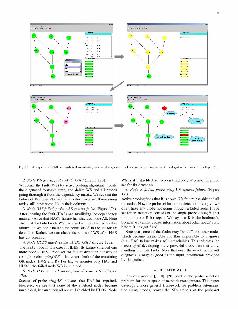
18

Fig. 16. A sequence of RAIL screenshots demonstrating successful diagnosis of a Database Server fault in our testbed system demonstrated in Figure 2.

2. Node WS failed, probe pWS failed (Figure 17b).We locate the fault (WS) by active probing algorithm, updatethe diagnosed system’s state, and delete WS and all probesgoing thorough it from the dependency matrix. We see that thefailure of WS doesn’t shield any nodes, because all remainingnodes still have some 1’s in their columns.

3. Node HAS failed, probe pAS returns failed (Figure 17c).After locating the fault (HAS) and modifying the dependencymatrix, we see that HAS’s failure has shielded node AS. Notealso, that the failed node WS has also become shielded by thisfailure. So we don’t include the probe pWS in the set for fixdetection. Rather, we can check the status of WS after HAShas got repaired.

4. Node HDBS failed, probe pDBS failed (Figure 17d).The faulty node in this case is HDBS. Its failure shielded onemore node - DBS. Probe set for failure detection consists ofa single probe - pingWS - that covers both of the remainingOK nodes (HWS and R). For fix, we monitor only HAS andHDBS; the failed node WS is shielded.

5. Node HAS repaired, probe pingAS returns OK (Figure17e).Success of probe pingAS indicates that HAS has repaired.However, we see that none of the shielded nodes becameunshielded, because they all are still shielded by HDBS. Node

WS is also shielded, so we don’t include pWS into the probeset for fix detection.

6. Node R failed, probe pingWS returns failure (Figure17f).Active probing finds that R is down. R’s failure has shielded allthe nodes. Now the probe set for failure detection is empty - wedon’t have any probe not going through a failed node. Probeset for fix detection consists of the single probe - pingR, thatmonitors node R for repair. We say that R is the bottleneck,because we cannot update information about other nodes’ statebefore R has got fixed.

Note that some of the faults may ”shield” the other nodeswhich become unreachable and thus impossible to diagnose(e.g., HAS failure makes AS unreachable). This indicates thenecessity of developing more powerful probe sets that allowhandling multiple faults. Note that even the exact multi-faultdiagnosis is only as good as the input information providedby the probes.

X. RELATED WORK

Previous work [9], [10], [28] studied the probe selectionproblem for the purpose of network management. This paperdevelops a more general framework for problem determina-tion using probes, proves the NP-hardness of the probe-set

19

(a) (b)

(c) (d)

(e) (f)

Fig. 17. Illustration of sequential multifault algorithm.

20

selection problem, develops the active probing approach anddemonstrates its advantages in reducing probe-set size.

Event correlation [5], [6] for identifying root-causes haslong been recognized as a critical issue in the system man-agement domain. Problem determination is performed by an-alyzing alarms emitted by devices when a significant situationoccurs. Unlike the probing scheme, alarms are “reactive”to a situation and this requires intensive instrumentation,only possible in a tightly managed environment. The probingapproach uses test transactions that can be built easily withouttouching the existing devices.

Nonetheless, event correlation has many similarities to ourwork. The formulation of problem diagnosis as a “decoding”problem, where “problem events” are decoded from “symp-tom events”, was first proposed by [7]. Our approach usesan active probing approach versus a “passive” analysis ofsymptom events; namely [7] selects codebooks (a combinationof symptoms encoding particular problems) from a specifiedset of symptoms, while we actively construct those symptoms(probes), a much more flexible approach. Another importantdifference is that [7] lacks a detailed discussion of efficientalgorithms for constructing optimal codebooks.

Other approaches to fault diagnosis in communication net-works and distributed computer systems include Bayesiannetworks [29], [1] and other probabilistic dependency mod-els [30]; another approach is statistical learning to detectdeviations from the normal behavior of the network [31].However the probe selection problem and active probing asformulated here were not addressed in that work. A compre-hensive treatment of multi-fault, including most-informativetest selection, was also provided in [22]. However, to thebest of our knowledge, combining probabilistic inference withonline selection of most-informative probes appears to be anovel approach in the area of distributed systems diagnosisvia end-to-end probing.

In our recent work [1], [10], a theoretical bound on thediagnostic error was derived; this lower bound provides nec-essary conditions for the number of probes needed to achievean asymptotically error-free diagnosis as the network sizeincreases, given prior fault probabilities and a certain levelof noise in probe outcomes. Also, empirical observationssuggested that a simple greedy approximation algorithm forfinding most-likely diagnosis (MPE) yield nearly-optimal re-sults when noise is sufficiently small. In this paper, we providea theoretical justification of these results.

XI. CONCLUSIONS

This paper addresses real-time problem diagnosis in com-puter networks and distributed computer systems. We im-prove the state-of-art by introducing a more adaptive andcost-efficient technique, called active probing. Active probinguses an information-theoretic approach to probe selection thatspeeds up real-time diagnosis by minimizing set of measure-ments, such as probes (test transactions), while maintaininghigh diagnostic accuracy.

We compare the existing pre-planned probe-selection ap-proach [9], [10] with the active probing. In the pre-planned

approach, a set of probes is selected and scheduled to runperiodically. Problem diagnosis is performed by analyzing theprobe results. This approach may be quite inefficient since itrequires running an unnecessarily large set of probes capableof diagnosing all possible problems, many of which mightin fact never occur. We prove that both problems of optimalprobe set selection for fault detection and for fault diagnosisare NP-hard. We then review (and reformulate in information-theoretic framework) simple approximation techniques of [9],[10] that serve as a baseline for comparison with the proposedactive probing approach.

In active probing, a set of probes is selected to run periodi-cally as before, but only for the purpose of detecting when aproblem occurs. Whenever occurrence a problem is detectedby one or more of the probes, additional probes are sent outto obtain further information about the problem. As proberesults are received, belief about the system state is updatedusing probabilistic inference in a Bayesian network, and thenext most-informative probe is selected and sent. This processcontinues until the problem is diagnosed. We demonstratethrough both analysis and simulation that the active probingscheme greatly reduces both the number of probes (by up to75% in our real-life applications and in simulations) and thetime needed for localizing the problem when compared withnon-adaptive, pre-planned probing schemes.

We discuss probabilistic inference approach to analyzingprobe results: a simple one based on k-fault assumption, anda generic multi-fault approach; we also provide theoreticalguarantees on diagnostic quality of a simple approximateinference algorithm in the presence of noise in probe out-comes. These encouraging results suggest the applicability ofsuch approximations to certain almost-deterministic diagnosticproblems that often arise in practical applications. Moreover,we demonstrate initial results on learning parameters of Dy-namic Bayesian Network from probe outcomes that allowsonline adaptation of diagnostic engine to system’s dynamics.Since inference in DBNs is generally intractable, we alsopresent an efficient approximate approach called sequentialmultifault that works well under certain restricting assumptions(such as single-node failure or repair in a system at a time);empirical results demonstrate clear advantage of such ap-proaches over ”static” techniques that do not handle system’schanges. Finally, we describe an architecture and functionalityof our proof-of-concept system that implements our approach.

Directions for future work include incorporating DynamicBayesian Network model into active probing in order to betterhandle system dynamics, such as intermittent faults, dynamicrouting and lack of precise knowledge of the probe path, andadapting to non-stationary behavior of the system using on-line learning that yields a dynamic, adaptive, probing strategy.We feel that adaptive, cost-effective techniques for problemdetermination will become increasingly important if new-generation IT systems are to be capable of self-managementand self-repair.

ACKNOWLEDGEMENTS

We would like to thank Vittorio Castelli, Daniel Oblingerand other members of the Machine-Learning group for many

21

insightful discussions that contributed to the ideas of thispaper. We also thank EPP team, especially Herb Lee, AndyFrenkiel, and Marius Sabbath, for their collaboration onRAIL/EPP framework, and Douglas Griswold, Luis Moss, andJustin Ellis for providing the data and useful information aboutvarious practical issues related to probing.

REFERENCES

[1] I. Rish, M. Brodie, and S. Ma, “Accuracy vs. Efficiency Trade-offsin Probabilistic Diagnosis,” in Proceedings of AAAI-2002, Edmonton,Alberta, Canada, 2002.

[2] M. Brodie, I. Rish, S. Ma, and N. Odintsova, “Active probing strategiesfor problem diagnosis in distributed systems,” in Proceedings of theThe Eighteenth International Joint Conference on Artificial Intelligence(IJCAI-03), Acapulco, Mexico, 2003.

[3] I. Rish, M. Brodie, N. Odintsova, S. Ma, and G. Grabarnik, “Real-timeProblem Determination in Distributed Systems using Active Probing,” inProceedings of 2004 IEEE/IFIP Network Operations and ManagementSymposium (NOMS 2004), Seoul, Korea, 2004.

[4] N. Odintsova, I. Rish, and S. Ma, “Multifault Diagnosis in DynamicSystems,” in Integrated management (IM-2005), Nice, France, 2005.

[5] A. Leinwand and K. Fang-Conroy, Network Management: A PracticalPerspective, 2nd Edition. Addison-Wesley, 1995.

[6] B. Gruschke, “Integrated Event Management: Event Correlation UsingDependency Graphs,” in DSOM, 1998.

[7] S. Kliger, S. Yemini, Y. Yemini, D. Ohsie, and S. Stolfo, “A codingapproach to event correlation,” in Intelligent Network Management (IM),1997.

[8] A. Frenkiel and H. Lee, “EPP: A Framework for Measuring the End-to-End Performance of Distributed Applications,” in Proceedings ofPerformance Engineering ’Best Practices’ Conference, IBM Academyof Technology, 1999.

[9] M. Brodie, I. Rish, and S. Ma, “Optimizing probe selection for faultlocalization,” in Distributed Systems Operation and Management, 2001.

[10] I. Rish, M. Brodie, and S. Ma, “Intelligent probing: a Cost-EfficientApproach to Fault Diagnosis in Computer Networks,” IBM SystemsJournal, vol. 41, no. 3, pp. 372–385, 2002.

[11] R. M. Karp, Complexity of Computer Computations. Plenum Press,1972, ch. Reducibility among combinatorial problems, pp. 85–103.

[12] M. Garey and D. Johnson, Computers and Intractability; A Guide to theTheory of NP-completeness. W.H. Freeman and Co., San Francisco,1979.

[13] T. Cover and J. Thomas, Elements of information theory. NewYork:John Wiley & Sons, 1991.

[14] J. Pearl, Probabilistic Reasoning in Intelligent Systems. MorganKaufmann, 1988.

[15] G. Cooper, “The computational complexity of probabilistic inferenceusing Bayesian belief networks,” Artificial Intelligence, vol. 42, no. 2–3, pp. 393–405, 1990.

[16] S. Lauritzen and D. Spiegelhalter, “Local computation with probabilitieson graphical structures and their application to expert systems,” Journalof the Royal Statistical Society, Series B, vol. 50(2), pp. 157–224, 1988.

[17] N. Zhang and D. Poole, “Exploiting causal independence in Bayesiannetwork inference,” Journal of Artificial Intelligence Research, vol. 5,pp. 301–328, 1996.

[18] R. Dechter, “Bucket elimination: A unifying framework for probabilisticinference,” in Proc. Twelfth Conf. on Uncertainty in Artificial Intelli-gence, 1996, pp. 211–219.

[19] R. Dechter and I. Rish, “A scheme for approximating probabilistic infer-ence,” in Proc. Thirteenth Conf. on Uncertainty in Artificial Intelligence(UAI97), 1997.

[20] ——, “Mini-buckets: A General Scheme for Approximating Inference,”J. of ACM, no. 50(2), pp. 107–153, 2003.

[21] J. Yedidia, W. T. Freeman, and Y. Weiss, “Generalized belief propaga-tion,” in NIPS 13. MIT Press, 2001, pp. 689–695.

[22] J. de Kleer and B. Williams, “Diagnosing Multiple Faults,” ArtificialIntelligence, vol. 32, no. 1, 1987.

[23] K. Murphy and Y. Weiss, “The factored frontier algorithm for approxi-mate inference in dbns,” in Proceedings of UAI-2001, 2001.

[24] X. Boyen and D. Koller, “Tractable inference for complex stochasticprocesses,” in Proceedings of the 14th Annual Conference on Uncer-tainty in AI (UAI-98), 1998, pp. 33–42.

[25] A. Dempster, N. Laird, and D. Rubin, “Maximum Likelihood fromIncomplete Data via The EM Algorithm,” Journal of Royal StatisticalSociety, vol. 39, pp. 1–38, 1977.

[26] K. Murphy, “Bayes net toolbox for matlab,” http://www.ai.mit.edu/ mur-phyk/Software/BNT/bnt.html.

[27] N. Odintsova, I. Rish, and S. Ma, “Multifault Diagnosis in DynamicSystems,” IBM T.J. Watson Research Center, Tech. Rep. RC23385,2004.

[28] H. Ozmutlu, N. Gautam, and R. Barton, “Zone recovery methodology forprobe-subset selection in end-to-end network monitoring,” in NetworkOperations and Management Symposium, 2002, pp. 451–464.

[29] J. Huard and A. Lazar, “Fault isolation based on decision-theoretictroubleshooting,” Center for Telecommunications Research, ColumbiaUniversity, New York, NY, Tech. Rep. 442-96-08, 1996.

[30] I.Katzela and M.Schwartz, “Fault identification schemes in communica-tion networks,” in IEEE/ACM Transactions on Networking, 1995.

[31] C. Hood and C. Ji, “Proactive network fault detection,” in Proceedingsof INFOCOM, 1997.

APPENDIX AHere we prove that PROBE-SET SELECTION FOR FAULT DIAGNO-

SIS is NP-hard.Proof: We will show that PROBE-SET SELECTION FOR FAULT

DIAGNOSIS is NP-hard via a reduction from PROBE-SET SELECTIONFOR FAULT DETECTION.

Let the dependency matrix DT,F and the positive integer kbe an arbitrary instance of PROBE-SET SELECTION FOR FAULTDETECTION. We need to construct, in polynomial time, sets F̂, T̂,and an integer k̂ ≤ |T̂|, such that there exists a subset of T of sizeat most k covering F if and only if there exists a subset of T̂ ofsize at most k̂ such that DT̂,F̂ has unique columns.

We assume there are m possible faults, i.e. F = {F1, . . . , Fm}.The set F̂ contains all the elements of F plus m new elementsG1, . . . , Gm. The set T̂ will contain all the probes in T, plus madditional probes {Fi, Gi} for all i ∈ {1, . . . , m}. The resultingdependency matrix will be of size (r+m)×(2m). It can be visualizedas the four-block matrix »

DT,F 0Im Im

–,

where Im denotes the m × m identity matrix. We also set k̂ =k + m − 1 (for reasons that will become clear later). It is easy tosee that the reduction can be done in polynomial time. We now showboth the sufficient and necessary conditions.

For the “if” direction, we assume that 〈DT,F, k〉 ∈PROBE-SET SELECTION FOR FAULT DETECTION, thus there exists asubset T′ ⊆ T of size at most k such that DT′,F has at least one1 in every column. We need to show that 〈DT̂,F̂, k̂〉 is a positiveinstance of PROBE-SET SELECTION FOR FAULT DIAGNOSIS. Indeed,there exists a subset Q of at most rows k̂ rows inducing a sub-matrix of DT̂,F̂ with unique columns – namely, Q contains T′ andany (m − 1) of the m additional rows {Fi, Gi}. Since DT′,F hasa 1 in every column, every column of DQ,F̂ corresponding to afault in F will differ from any column corresponding to a fault in{G1, . . . , Gm}. Since removing a single row from Im leaves all them columns distinct, the columns corresponding to the elements of Fwill all be distinct from each other, as are the columns correspondingto the elements of {G1, . . . , Gn}. Notice that |Q| ≤ k+m−1 = k̂,as desired.

To show the other direction, we assume that 〈DT,F, k〉 is a nega-tive instance of PROBE-SET SELECTION FOR FAULT DETECTION. Weneed to show that 〈DT̂,F̂, k̂〉 will be a negative instance of PROBE-SET SELECTION FOR FAULT DIAGNOSIS. Indeed, if any subset of atmost k rows of DT,F induces an all-0 column, then any submatrix ofDT̂,F̂ induced by a subset of at most k̂ rows will contain duplicatecolumns. To see this, let Q be a subset of at most k̂ rows. There aretwo cases to be considered:

1) Q contains at most k elements of T. Then, since there is anall-0 column in DT,F induced by Q∩T, we know that DQ,F̂

22

will have identical columns corresponding to faults Fi and Gi,where i is the index of the all-0 column in DT,F.

2) Q contains more than k elements of T. In this case Q cannotcontain more than m − 2 of the new rows (since |Q| ≤ k̂).But then Q will induce duplicate columns in the right halfof DT̂,F̂, since removing at least two rows from Im inducesduplicate columns.

Thus any subset Q of at most k̂ rows induces duplicate columns inDT̂,F̂, making it a negative instance of PROBE-SET SELECTION FORFAULT DIAGNOSIS, as desired.

APPENDIX B

Here we derive the equation 4 for I(X; T ). Here X ∈ {0, 1, ..., n}denotes the state of the system under the single-fault assumption,where X = 0 corresponds to the no-fault situation, and X = icorresponds to failure of node Xi. A particular prior distributionP (X) is assumed where P (X = 0) = 1 − p, and the probabilityof fault in the system, p, is uniformly distributed over the nodes, i.e.P (X = i) = p/n where 1 ≤ i ≤ n. We assume that T is a probeof length k, and that T = 0 denotes probe’s success, while T = 1denotes probe’s failure. Note that I(X; T ) = H(X) − H(X|T ),where

H(X) = −(1− p) log(1− p)− np

nlog

p

n=

= −(1− p) log(1− p)− p logp

n, and (9)

−H(X|T ) =Xt,x

P (x, t) log P (x|t) =

=X

t

P (t)X

x

P (x|t) log P (x|t). (10)

Due to single-fault assumption, a probe T of length k fails if exactlyone of its nodes fail, yielding a union of k mutually exclusive nodefailure events, each having probability p/n. Therefore,

P (T = 1) =kp

n, and P (T = 0) = 1− kp

n=

n− kp

n. (11)

Next,

P (X = 0|T = 1) = 0,

P (X = 0|T = 0) =P (X = 0, T = 0)

P (T = 0)=

P (X = 0)

P (T = 0)=

=1− p

1− kp/n=

n(1− p)

n− kp, (12)

since X = 0 is the intersection of events X = 0 and T = 0 (i.e.,the event X = 0, T = 0).

Let us now compute P (X = i|T ) for 1 ≤ i ≤ n, and T ∈{0, 1}. We will consider two cases: when Xi belongs to the probeT , and when it does not. We will abuse the notation slightly, andsay Xi ∈ T if Xi is on the path of probe T . Then, we can computeP (X = i|T ) = P (X = i, Xi ∈ T |T ) + P (X = i, Xi /∈ T |T ) asfollows:

P (X = i, Xi ∈ T |T = 0) =P (X = i, Xi ∈ T, T = 0)

P (T = 0)= 0,

P (X = i, Xi /∈ T |T = 0) =P (X = i, Xi /∈ T, T = 0)

P (T = 0)=

=P (X = i)

P (T = 0)=

p

n− kp, (13)

since the intersection of events X = i, Xi ∈ T, T = 0 is empty(incompatible events), and the intersection of events X = i, Xi /∈

T, T = 0 is simply X = i. Similarly,

P (X = i, Xi ∈ T |T = 1) =P (X = i, Xi ∈ T, T = 1)

P (T = 1)=

=P (X = i)

P (T = 1)=

p/n

kp/n= 1/k,

P (X = i, Xi /∈ T |T = 1) =P (X = i, Xi /∈ T, T = 1)

P (T = 1)= 0,

since the intersection of events X = i, Xi ∈ T, T = 1 is simplyX = i, and the intersection of events X = i, Xi /∈ T, T = 1 isempty (incompatible events).

Now, we can combine the equations above to compute thenegative conditional entropy in 10. We decompose P (X|T ) intosum over a set mutually exclusive events, (1) X = 0, and (2){X = i, i > 0}, where each event X = i, i > 0 can be furtherpartitioned into X = i, Xi ∈ T, i > 0 and X = i, Xi /∈ T, i > 0.As the result, we get the following expression for −H(X|T ):X

t∈{0,1}P (T = t)

X

i∈{0,1,...,n}P (X = i|T = t) log P (X = i|T = t) =

=X

t∈{0,1}P (T = t)

ˆP (X = 0|T = t) log P (X = 0|T = t)+

+X

i∈{1,...,n}

ˆP (X = i, X ∈ T |T = t)+

+P (X = i, X /∈ T |T = t)˜log P (X = i|T = t)

˜˜=

=n− kp

n

ˆn(1− p)

n− kplog

n(1− p)

n− kp+ k · 0+

+(n− k)p

n− kplog

p

n− kp

˜+

+kp

n

ˆ0 + k

1

klog

1

k+ (n− k) · 0˜ =

= (1− p) log1− p

1− k pn

+ (n− k)p

nlog

p

n− kp− k

p

nlog k. (14)

Substituting the expression 14 for −H(X|T ) in 10 and combiningit with th the equations 9, we get exactly the equation 4:

I(X; T ) = I(p, n, k) = −(1− p) log(1− p)− p logp

n

−kp

nlog k + (1− p) log

1− p

1− k pn

+ (n− k)p

nlog

p

n− pk.