Incremental Adaptive Strategies Over Distributed Networks

4064 IEEE TRANSACTIONS ON SIGNAL PROCESSING, VOL. 55, NO. 8, AUGUST 2007

Incremental Adaptive Strategies OverDistributed Networks

Cassio G. Lopes, Student Member, IEEE, and Ali H. Sayed, Fellow, IEEE

Abstract—An adaptive distributed strategy is developed basedon incremental techniques. The proposed scheme addresses theproblem of linear estimation in a cooperative fashion, in whichnodes equipped with local computing abilities derive local es-timates and share them with their predefined neighbors. Theresulting algorithm is distributed, cooperative, and able to re-spond in real time to changes in the environment. Each node isallowed to communicate with its immediate neighbor in order toexploit the spatial dimension while limiting the communicationsburden at the same time. A spatial–temporal energy conservationargument is used to evaluate the steady-state performance of theindividual nodes across the entire network. Computer simulationsillustrate the results.

Index Terms—Adaptive networks, consensus, cooperation, dif-fusion algorithm, distributed processing, incremental algorithm.

I. INTRODUCTION

DISTRIBUTED processing deals with the extraction of in-formation from data collected at nodes that are distributed

over a geographic area. For example, each node in a networkof nodes could collect noisy observations related to a certainparameter or phenomenon of interest. The nodes would then in-teract with their neighbors in a certain manner, as dictated bythe network topology, in order to arrive at an estimate of theparameter or phenomenon of interest. The objective is to arriveat an estimate that is as accurate as the one that would be ob-tained if each node had access to the information across the en-tire network. In comparison, in a traditional centralized solution,the nodes in the network would collect observations and sendthem to a central location for processing. The central processorwould then perform the required estimation tasks and broad-cast the result back to the individual nodes. This mode of opera-tion requires a powerful central processor, in addition to exten-

Manuscript received February 27, 2006; revised November 28, 2006. Theassociate editor coordinating the review of this manuscript and approving it forpublication was Prof. Jonathon Chambers. This material was based on work sup-ported in part by the National Science Foundation under awards ECS-0401188and ECS-0601266. The work of C. G. Lopes was also supported by a fellow-ship from CAPES, Brazil, under award 1168/01-0. A short version of this workappeared in Proceedings of the IEEE International Conference on Acoustics,Speech and Signal Processing (ICASSP), Toulouse, France, May 2006, vol. 3,pp. 584–587.

The authors are with the Department of Electrical Engineering, Universityof California, Los Angeles, CA 90095 USA (e-mail: [email protected];[email protected]).

Color versions of one or more of the figures in this paper are available onlineat http://ieeexplore.ieee.org.

Digital Object Identifier 10.1109/TSP.2007.896034

Fig. 1. Distributed network with N nodes accessing temperature data.

Fig. 2. Monitoring a diffusion phenomenon by a network of sensors deployedin the field.

sive amounts of communication between the nodes and the pro-cessor. In the distributed solution, the nodes rely solely on theirlocal data and on interactions with their immediate neighbors.The amount of processing and communications is significantlyreduced [1]–[3].

A. Applications

Let us illustrate these ideas with an example. Consider a col-lection of nodes spread over a geographic area, as shown inFig. 1. Each node has access to a local temperature measurement

. The objective is to provide each node with information aboutthe average temperature across the network. In one distributedsolution to this problem (known as a consensus implementation[4]–[6]), each node combines the measurements from its imme-diate neighbors (those that are connected to it). The result of thecombination becomes this node’s new measurement, i.e.,

node 1

where denotes the updated measurement of node 1 at iter-ation , and the ’s are appropriately chosen coefficients. Everyother node in the network performs the same operation and theprocess is repeated. Under suitable conditions on the ’s andnetwork topology, all node measurements will converge asymp-totically to the desired average temperature .

A more sophisticated application is to use measurements col-lected in time and space by a group of sensors in order to monitorthe concentration of a chemical in the air or water (see Fig. 2).

1053-587X/$25.00 © 2007 IEEE

LOPES AND SAYED: INCREMENTAL ADAPTIVE STRATEGIES OVER DISTRIBUTED NETWORKS 4065

Fig. 3. Three modes of cooperation: (a) Incremental; (b) diffusion; and (c)probabilistic diffusion.

These measurements can then be used to estimate the parame-ters of the model that dictates the diffusion of thechemical in the environment according to some diffusion equa-tion subject to boundary conditions, e.g.,

where denotes the concentration at location at time[7]. Another application of distributed processing is monitoringa moving target in a region monitored by a collection of sensors[8]. The sensors would share their noisy measurements throughlocal interactions in order to detect the presence of the target andtrack its trajectory.

Such distributed networks linking PCs, laptops, cell phones,sensors, and actuators will form the backbone of future datacommunication and control networks. Applications will rangefrom sensor networks to precision agriculture, environmentmonitoring, disaster relief management, smart spaces, targetlocalization, as well as medical applications [1], [8]–[10]. In allthese cases, the distribution of the nodes in the field yields spa-tial diversity, which should be exploited alongside the temporaldimension in order to enhance the robustness of the processingtasks and improve the probability of signal and event detection[1].

B. Modes of Cooperation

Obviously, the effectiveness of any distributed implementa-tion will depend on the modes of cooperation that are allowedamong the nodes. Fig. 3 illustrates three such modes of cooper-ation.

In an incremental mode of cooperation, information flowsin a sequential manner from one node to the adjacent node.This mode of operation requires a cyclic pattern of collabora-tion among the nodes, and it tends to require the least amountof communications and power [2], [11], [12]. In a diffusion im-plementation, on the other hand, each node communicates withall its neighbors as dictated by the network topology [13]–[15].The amount of communication in this case is higher than inan incremental solution. Nevertheless, the nodes have access tomore data from their neighbors. The communications in the dif-fusion implementation can be reduced by allowing each node tocommunicate only with a subset of its neighbors. The choice ofwhich subset of neighbors to communicate with can be random-ized according to some performance criterion. In this paper, wefocus on the incremental mode of collaboration.

C. Consensus Strategy

The temperature example that we mentioned before is a spe-cial case of a more general strategy for distributed processing,known as consensus (e.g., [4]–[6], and [16]). Broadly, consensusimplementations employ two time scales and they function asfollows. Assume the network is interested in estimating a cer-tain parameter. Each node collects observations over a periodof time and reaches an individual decision about the parameter.During this time, there is limited interaction among the nodes;the nodes act more like individual agents. Following this initialstage, the nodes then combine their estimates through severalconsensus iterations; under suitable conditions, the estimatesgenerally converge asymptotically to the desired (global) esti-mate of the parameter.

Let us consider another example of a consensus implementa-tion, which will serve as further motivation for the contributionsin this work. Consider again a collection of nodes. Each nodehas access to a data vector and a data matrix . The arenoisy and distorted measurements of some unknown vector ,as follows:

Each node can evaluate the least-squares estimate of basedon its own local data . To do so, each node evaluatesits local cross-correlation vector and its autocor-relation matrix . Then, the local estimate ofcan be found from . This operation requires thateach node collects sufficient data into and . Once the localquantities have been evaluated at the individual nodes,one can apply consensus iterations at the nodes to determineand , which are estimates of the overall (mean) quantitiesand defined by [13], as follows:

and

A global estimate of is given by . For all prac-tical purposes, a least-squares implementation in this manner isan offline or nonrecursive solution. For example, if a particularnode collects one more entry in and one more row in , adifficulty that occurs is how to update the current solution toaccount for new data without having to repeat prior processingand iterations afresh. In addition, the offline averaging limits theability of consensus-based solutions to track fast-changing en-vironments, especially in networks with limited communicationresources.

D. Contributions

To address the aforementioned issues (need for adaptiveimplementations, real-time operation, and low computationaland communications complexity), we propose a distributedleast-mean-squares (LMS)-like algorithm that requires lesscomplexity for both communications and computations andinherits the robustness of LMS implementations [17]. Theproposed solution promptly responds to new data, as theinformation flows through the network. It does not requireintermediate averaging as in consensus implementations; it


neither requires two separate time scales. The distributedadaptive solution is an extension of adaptive filters and can beimplemented without requiring any direct knowledge of datastatistics; in other words, it is model independent. While wefocus in this paper on LMS-type updates for simplicity, thesame ideas and techniques apply to other types of adaptationrules.

Our objective is therefore to develop distributed algorithmsthat enable a network of nodes to function as an adaptive entityin its own right. Thus, recall that a regular adaptive filter re-sponds in real time to its data and to variations in the statisticalproperties of this data. We want to extend this ability to the net-work domain [12], [18], [19]. Specifically, the purpose of thispaper is threefold:

1) to motivate a family of incremental adaptive algorithms fordistributed estimation inspired by distributed optimizationtechniques [2], [20], [21];

2) to use the incremental algorithms to propose an adaptivenetwork structure composed of an interconnected set ofnodes that is able to respond to data in real time and totrack variations in the statistical properties of the data asfollows:

a) each time a node receives a new piece of information,this information is readily used by the node to updateits local estimate of the parameter of interest;

b) the local estimates of the parameter are shared withthe immediate neighbors of the node in a process thatallows the information to flow to other nodes in thenetwork;

3) to analyze the performance of the resulting interconnectednetwork of nodes. This task is challenging since an adap-tive network comprises a “system of systems” that pro-cesses data cooperatively in both time and space. Differentnodes will converge to different mean-square-error (MSE)levels, reflecting the statistical diversity of the data and thedifferent noise levels.

In summary, we propose an incremental adaptive algorithmover ring topologies and derive closed form expressions for itsmean-square performance.

E. Notation and Paper Organization

In this paper, we need to distinguish not only between vectorsand matrices, but also between random and nonrandom quanti-ties (see, e.g., [17]). Thus, we adopt boldface letters for randomquantities and normal font for nonrandom (deterministic) quan-tities. We also use capital letters for matrices and small lettersfor vectors. For example, is a random observation quantity,and is a realization or measurement for it, and is a covari-ance matrix while is a weight vector. The notation is used todenote complex conjugation for scalars and complex-conjugatetransposition for matrices.

The paper is organized as follows. In Section II, a distributedestimation problem is formulated and a framework for dis-tributed adaptive processing is described, with the subsequentderivation of a distributed incremental LMS algorithm. InSection III, the performance of the temporal and spatial adap-tive strategy is studied, providing closed-form expressions forthe mean-square behavior of the distributed algorithm. The

Fig. 4. Distributed network withN active nodes accessing space–time data.

theoretical results are compared with simulations in Section IV.Section V points out future extensions that are currently beingdeveloped.

II. ESTIMATION PROBLEM AND THE ADAPTIVE

DISTRIBUTED SOLUTION

There have been extensive works in the literature on incre-mental methods for solving distributed optimization problems(e.g., [2], [11], [20], [22], and [23]). It is known that whenevera cost function can be decoupled into a sum of individual costfunctions, a distributed algorithm can be developed for mini-mizing the cost function through an incremental procedure. Weexplain the procedure as follows in the context of MSE estima-tion.

Consider a network with nodes (see Fig. 4). Each nodehas access to time realizations of zero-mean spa-tial data , , where each is a scalarmeasurement and each is a row regression vector.We collect the regression and measurement data into two globalmatrices, as follows:

(1)

(2)

These quantities collect the data across all nodes. The objec-tive is to estimate the vector that solves

(3)

where the cost function denotes the MSE, as follows:

(4)

and is the expectation operator. The optimal solution of(3) satisfies the orthogonality condition [17]

(5)

so that is the solution to the normal equations

(6)

which are defined in terms of the correlation and cross-correla-tion quantities

(7)

If the optimal solution were to be computed from (6), thenevery node in the network would need to have access to theglobal statistical information . Alternatively, the so-lution could be computed centrally and the result broadcast


to all nodes. Either way, these approaches drain considerablecommunications and computational resources and they do notendow the network with the necessary adaptivity to cope withpossible changes in the statistical properties of the data.

We shall instead develop and study a distributed solution thatallows cooperation among the nodes through limited local com-munications, while at the same time equipping the network withan adaptive mechanism [12]. Specifically, in this paper we focuson the incremental mode of cooperation, where the estimationtask is distributed among the nodes and each node is allowed tocooperate only with one of its direct neighbors at a time. Thesingle-neighbor case is already challenging in its own right, andthe analysis will bring forth several interesting observations. Ex-tensions to other modes of cooperation are possible [15], [18],[19].

A. Steepest-Descent Solution

To arrive at the adaptive distributed solution we first reviewthe steepest-descent solution and its incremental implementa-tion. To begin with, we note from (4) and (7) that the cost func-tion can be decomposed as

(8)

where each is given by

(9)

(10)

and the second-order moment quantities are defined by

and(11)

In other words, can be expressed as the sum of indi-vidual cost functions , one for each node . Thus, the tra-ditional iterative steepest-descent solution for determiningcan be expressed in the form

initial condition

(12)

where is a suitably chosen positive step-size parameter,is an estimate for at iteration , and denotes

the gradient vector of with respect to evaluated at .For sufficiently small, we will have asfor any initial condition. An equivalent implementation can bemotivated as follows.

Let us define a cycle visiting every node over the networktopology only once such that each node has access only to itsimmediate neighbor node in this cycle [2], [11], [21]. Let

Fig. 5. Data processing in the proposed adaptive distributed structure.

denote a local estimate of at node at time . Thus, assumethat node has access to , which is an estimate of atits immediate neighbor node in the defined cycle (seeFig. 5). If at each time instant we start with the initial condition

at node 1 (i.e., with the current global estimatefor ), and iterate cyclicly across the nodes then, at the

end of the procedure, the local estimate at node will coincidewith from (12), i.e., . In other words, the followingimplementation is equivalent to (12):

(13)

Observe that in this steepest-descent implementation, the itera-tion for is over the spatial index .

B. Incremental Steepest-Descent Solution

Although recursion (13) is cooperative in nature, with eachnode using information from its immediate neighbor (repre-sented by ), this implementation still requires the nodes tohave access to the global information in order to evaluate

. This fact undermines our stated objective of a fullydistributed solution.

In order to resolve this difficulty, we call upon the concept ofincremental gradient algorithms [11], [20], [21]. If each nodeevaluates the required partial gradient at the local esti-mate received from node , as opposed to , thenan incremental version of algorithm (13) would result, namely

(14)This cooperative scheme relies only on locally available in-

formation, leading to a truly distributed solution. The schemerequires each node to communicate only with its immediateneighbor, thus saving on communication and energy resources[2], [11].

C. Incremental Adaptive Solution

The incremental solution (14) relies on knowledge of thesecond-order moments and , which are needed toevaluate the local gradients . An adaptive implementationof (14) can be obtained by replacing the second-order moments


by instantaneous approximations, say of theLMS type, as follows1:

(15)

by using data realizations at time . The approx-imations (15) lead to an adaptive distributed incremental algo-rithm, or simply a distributed incremental LMS algorithm of thefollowing form:

For each time repeat:

(16)

The operation of algorithm (16) is illustrated in Fig. 5. Ateach time instant , each node uses local data realizations

and the weight estimate received from itsadjacent node to perform the following three tasks:

1) evaluate a local error quantity: ;

2) update its weight estimate: ;

3) pass the updated weight estimate to its neighbor node.

This distributed incremental adaptive implementation generallyhas better steady-state performance and convergence rate thana nondistributed implementation that is based on using inplace of in the expression for (see Appendix A), i.e.,

(17)This is a reflection of a result in optimization theory that theincremental strategy (14) can outperform the steepest-descenttechnique (13), [20], [21]. Intuitively, this is because the incre-mental solution incorporates local information on-the-fly intothe operation of the algorithm, i.e., it exploits the spatial diver-sity more fully. While the steepest-descent solution (13) has

fixed throughout all spatial updates,the incremental solution (14) uses instead the successive up-dates . More detailed comparisons be-tween both implementations are provided in Appendix A.

In order to illustrate these observations, we run a simulationcomparing the excess mean-square error (EMSE) of the incre-mental adaptive algorithm (16) and the stochastic implementa-tion (17) at node 1, i.e., —see Figs. 6 and7. The network has nodes pursuing the same unknownvector , with , and relyingon independent Gaussian regressors with . The back-ground noise is white and Gaussian with , and weassume the data are related via for eachnode. The curves are obtained by averaging over 500 experi-ments. Fig. 6 shows the transient EMSE performance for both

1Other approximations are possible and they lead to alternative adaptationrules [17].

Fig. 6. Transient EMSE performance at node 1 for both incremental adaptivesolution (16) and stochastic steepest-descent solution (17).

Fig. 7. Steady-state EMSE performance at node 1 as �! 0 for both the incre-mental adaptive solution (16) and the stochastic steepest-descent solution (17).

algorithms, whereas Fig. 7 plots the steady-state values for de-creasing step sizes, obtained by averaging the last 1000 samplesafter convergence.

In terms of complexity, the incremental solution (16) requirescomputations per node and also scalar transmis-

sions per node. As such, the algorithm is intrinsically simple andis especially suitable for networks with low-energy resources.

III. PERFORMANCE ANALYSIS

An important question now is, how well does the adaptive in-cremental solution (16) perform? That is, how close does each

(local estimate at node ) get to the desired solutionas time evolves? Studying the performance of such an intercon-nected network of nodes is challenging (more so than studyingthe performance of a single LMS filter) for the following rea-sons:

1) each node is influenced by local data with local statistics(spatial information);

2) each node is influenced by its neighbors through the in-cremental mode of cooperation (spatial interaction);

3) each node is subject to local noise with variance (spa-tial noise profile).

In the next section, we provide a framework for studying theperformance of such network by examining the flow of energythrough the network both in time and space. For instance,we shall derive expressions that measure for each node thesteady-state values and as . Itwill be shown that despite the quite simple cooperation strategyadopted, in steady-state each individual node is affected by the


whole network, with some emphasis given to local statistics.Furthermore, as the step size is decreased asymptotically, bothquantities [mean-square deviation (MSD) and EMSE] approachzero for every node in the network, which also drives the MSEfor every node asymptotically to the background noise level

.In order to pursue the performance analysis, we shall rely on

the energy conservation approach of [17]. This energy-based ap-proach needs to be extended to account for the space dimensionbecause the distributed adaptive algorithm (16) involves botha time variable and a space variable . Moreover, we needto deal with the energy flow across interconnected filters andsince each node in the network can now stabilize at an individualMSE value, some of the simplifications that were possible inthe single node case [17] cannot be applied here. For example,due to cooperation, the performance of every node ends up de-pending on the whole network, an effect which we shall captureby a set of coupled equations. In order to evaluate individualnode performance, weighting will be used to decouple the equa-tions and to evaluate the quantities of interest in steady state.

The main result of this section is Theorem 1, further ahead,which provides closed-form expressions for the performance ofeach node in the network in terms of the so-called MSE, MSD,and EMSE measures defined next.

A. Data Model and Assumptions

To carry out the performance analysis, we first need to as-sume a model for the data as is commonly done in the literatureof adaptive algorithms. As indicated earlier, we denote randomvariables by boldface letters. Thus, are realizationsof the random quantities . The subsequent analysisassumes the following data model for :

A1) the desired unknown vector relates as

(18)

where is some temporally and spatially whitenoise sequence with variance and independent of

for all ;A2) is independent of for (spatial indepen-

dence);A3) is independent of for (time indepen-

dence).

Linear models of the form (18) arise in several applications [7],[13], [17], [24], [25]. The model (18) assumes that the networkis attempting to estimate an unknown vector . This is oftenreferred to as the stationary model. It captures the space di-mension by assigning different signals at differentnodes . The time dimension is accounted for by sequentiallyobserving the temporal evolution of such signals. The signals

can be regarded simply as observations and mea-surements, collected locally by the nodes or, for example, asexcitation/response pairs. The subsequent analysis can be ex-tended to handle nonstationary models where also varieswith time ([17], [26]). For space limitations, we study here only

the stationary case. Nevertheless, the distributed adaptive solu-tion (16) also applies to nonstationary scenarios. Moreover, asis common in the study of traditional adaptive filters, we areassuming that the regressors are spatially and temporally inde-pendent to simplify the analysis. However, the distributed adap-tive solution applies regardless of the assumptions, although theanalysis would be far more demanding.

B. Weighted Energy Conservation Relation

To proceed, we define the following local error signals at eachnode :

weight error vector at time (19)

a priori error (20)

a posteriori error (21)

output error (22)

It should be noted that we are using traditional terminology(e.g., as in [17]), except that now the terms “a priori” and“a posteriori” have a spatial connotation as opposed to tem-

poral connotation. The vector measures the differencebetween the weight estimate at node and the desired so-lution . The signal measures the estimation error inapproximating by using information available locally,i.e., . If were to converge to , then by (18)we would expect , so that the variance ofwould tend to . Thus, by evaluating how closegets to , we can estimate the performance of node . Notethat the error can be related to the a priori errorby using the data model (18) as

(23)

Hence, , so that evaluatingis useful for evaluating .

We are interested in evaluating the MSD, the MSE, and theEMSE in steady state for every node . These quantities aredefined as follows:

MSD (24)

EMSE (25)

MSE (26)

In order to arrive at expressions for these quantities, we shallfind it useful to resort to weighted norms as we now explain. In-troduce the weighted norm notation for a vector

and a Hermitian positive definite matrix . Then, underthe assumed data conditions we have that

(27)


In other words, we need to evaluate the means of two weighted

norms of in (27). To do so, we shall first establish thatthere is a fundamental spatio–temporal energy balance relatingthe error variables (19)–(21).

We start by defining weighted a priori and a posteriori localerror signals for each node as follows:

and (28)

for some Hermitian positive-definite matrix that we are freeto choose. As we shall see later, different choices for allow usto evaluate and examine different performance measures [17],[27]. We now seek an energy relation that compares the normsof the following error quantities:

(29)

Using algorithm (16) and subtracting from both sides gives

(30)

Multiplying the previous equation from the left by gives

(31)

so that from the definitions (28)

(32)

and, subsequently

(33)

Substituting (33) into (30) and rearranging terms, we get

(34)

Equating the weighted norm of both sides of (34), we find thatthe cross terms cancel out, and we end up with only energyterms, i.e.,

(35)

Equation (35) is a space–time version of the weighted energyconservation relation developed in [17] in the context of regularadaptive implementations. This is an exact relation that showshow the energies of several error variables are related to eachother in space and time. No approximations are used to derive(35).

C. Variance Relation

We now proceed to show how the energy conservation rela-tion can be used to evaluate the performance of each individualnode. First, we drop the time index for compactness of nota-tion. Then, we transform the relation (35) into a recursion of

by substituting (32) into (35) and rearranging terms, asfollows:

(36)Using (23) and taking expectations of both sides leads to

(37)

Using again the weighted error definitions (28), we can expand(37) in terms of weighted error vectors and the regressor data asfollows:

(38)

Now, given that , the previous equa-tion can be rewritten more compactly as

(39)

in terms of the stochastic weighting matrix

(40)

Invoking the independence of the regression data allowsus to write

(41)

so that (39) and (40) become

(42)

where is given by

(43)and is now a deterministic matrix.

D. Gaussian Data

Recursion (42) is a spatial variance relation that will allow usto evaluate the steady-state performance of every node . Notethat in (43) is solely regressor dependent, and, therefore, itsvalue is decoupled from (42). As a consequence, the study ofthe network behavior relies solely on the evaluation of the threedata moments, as follows:

and(44)

The evaluation of the third moment can be involved for non-Gaussian data [17]. In this paper, we assume Gaussian data


for simplicity. Thus, assume that the arise from a cir-cular Gaussian distribution and introduce the eigendecomposi-tion , where is unitary and is a diagonalmatrix with the eigenvalues of . Introduce further the trans-formed quantities

Since is unitary, we have that and, so that (42) and (43) can be rewritten in the

equivalent forms

(45)

(46)

The moments we need to evaluate are now , ,and . The first two moments are straightforwardsince

and (47)

The third moment is given for Gaussian regressors by [17]

(48)

where for circular complex data and for real data.Substituting (47) and (48) into the variance relation (45), (46)leads to

(49)

(50)

E. Diagonalization

Since is at our choice, we choose it such that both andwill become diagonal in (50). This suggests a more compact

notation in terms of the diagonal entries of and . Thus,introduce the column vectors

(51)

where the notation will be used in two ways:is a diagonal matrix whose entries are those of

the vector , and is a vector containing the maindiagonal of .

Using the diagonal notation, expression (50) can be rewrittenin terms of as

(52)

where the coefficient matrix is defined by

(53)

Moreover, expression (49) becomes

(54)

For the sake of compactness, the notation will bedropped from the subscripts in (54), keeping only the corre-sponding vectors

(55)

where we are restoring the time index for clarity, and weare replacing by in order to indicate that theweighting matrix can be node dependent.

F. Steady-State Behavior

Let and (a row vector). Then, for(i.e., in steady state), the variance relation (55) gives

(56)

We want to use this expression to evaluate the performance mea-sures, as follows:

MSD (57)

EMSE (58)

MSE (59)

with weighting vectors and . Observe, however, that (56) is acoupled equation: it involves both and , i.e., informationfrom two spatial locations. The ring topology together with theweighting matrices can be exploited to resolve this difficulty.

Thus, note that by iterating (56) we get a set of coupledequalities

...

(60)

...

(61)

These equations can be solved for via a suitable choiceof the free parameters and proper manipulation of theequations. Thus, note that (61) expresses in termsof . Then, choosing in


(60) gives

(62)so that

(63)

Iterating in this manner, we end up with an equality involvingonly , namely

(64)

It is convenient to define, for each node , a set of matricesin terms of products of matrices

(65)where the subscripts are all . The matrix can beinterpreted as the transition matrix that is necessary for theweighting vector to reach node cyclicly through nodes

. With this definition, we canrewrite (64) as

(66)

where the row vector is defined as

(67)

Likewise, the vector has the interpretation of the combinedeffect of transformed noise and local data statistics reachingnode from other nodes over the ring topology.

Recall that we wish to evaluate and. Thus, different choices of the weighting vector

in (66) should enable us to calculate the quantities thatdescribe the steady-state behavior of each node. Selecting theweighting vector as the solution of the linear equation

, we arrive at an expression for the desiredMSD:

MSD (68)

Likewise, for the EMSE, we choose the weighting vectoras the solution of so that

EMSE (69)

We summarize the results in the following theorem. Thestatement quantifies the performance of a spatio–temporaldistributed adaptive solution.

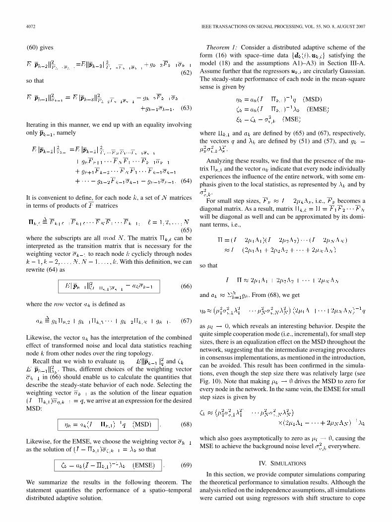
Theorem 1: Consider a distributed adaptive scheme of theform (16) with space–time data satisfying themodel (18) and the assumptions A1)–A3) in Section III-A.Assume further that the regressors are circularly Gaussian.The steady-state performance of each node in the mean-squaresense is given by

MSD

EMSE

MSE

where and are defined by (65) and (67), respectively,the vectors and are defined by (51) and (57), and

.

Analyzing these results, we find that the presence of the ma-trix and the vector indicate that every node individuallyexperiences the influence of the entire network, with some em-phasis given to the local statistics, as represented by and by

.For small step sizes, , i.e., becomes a

diagonal matrix. As a result, matrixwill be diagonal as well and can be approximated by its domi-nant terms, i.e.,

so that

and . From (68), we get

as , which reveals an interesting behavior. Despite thequite simple cooperation mode (i.e., incremental), for small stepsizes, there is an equalization effect on the MSD throughout thenetwork, suggesting that the intermediate averaging proceduresin consensus implementations, as mentioned in the introduction,can be avoided. This result has been confirmed in the simula-tions, even though the step size there was relatively large (seeFig. 10). Note that making drives the MSD to zero forevery node in the network. In the same vein, the EMSE for smallstep sizes is given by

which also goes asymptotically to zero as , causing theMSE to achieve the background noise level everywhere.

IV. SIMULATIONS

In this section, we provide computer simulations comparingthe theoretical performance to simulation results. Although theanalysis relied on the independence assumptions, all simulationswere carried out using regressors with shift structure to cope


with realistic scenarios. Therefore, the regressors are filled upas

(70)

In order to generate the performance curves, 100 independentexperiments were performed and averaged. The steady-statecurves are generated by running the network learning processfor 50 000 iterations. The quantities of interest, namely, MSD,EMSE, and MSE, are then obtained by averaging the last 5000samples of the corresponding learning curves. The measurementdata are generated according to the model (18) with the(unknown) vector set as .

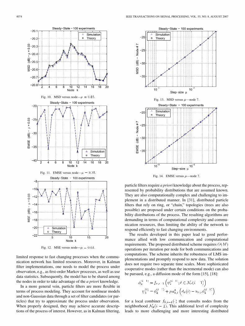
Two kinds of curves are presented. One kind depicts thesteady-state quantities as a function of the node for a partic-ular choice of the step size . These curves can be used to guidethe design of the network. For instance, they tell the designerhow to adjust the step-size at a certain node to compensatefor a signal power increase in nearby nodes. Or even, how thefilters are affected by a noise power increase at some nodes inthe network. A second kind of curve depicts the behavior ofthe steady-state quantities as a function of the step size for aparticular node. These curves evaluate the quality of the the-oretical model [17]. Usually, large deviations between theoryand simulation are expected for bigger step sizes: that is, whenthe simplifying assumptions adopted in the analysis are nolonger reasonable; therefore, curves like those in Figs. 13–15have a strong theoretical appeal.

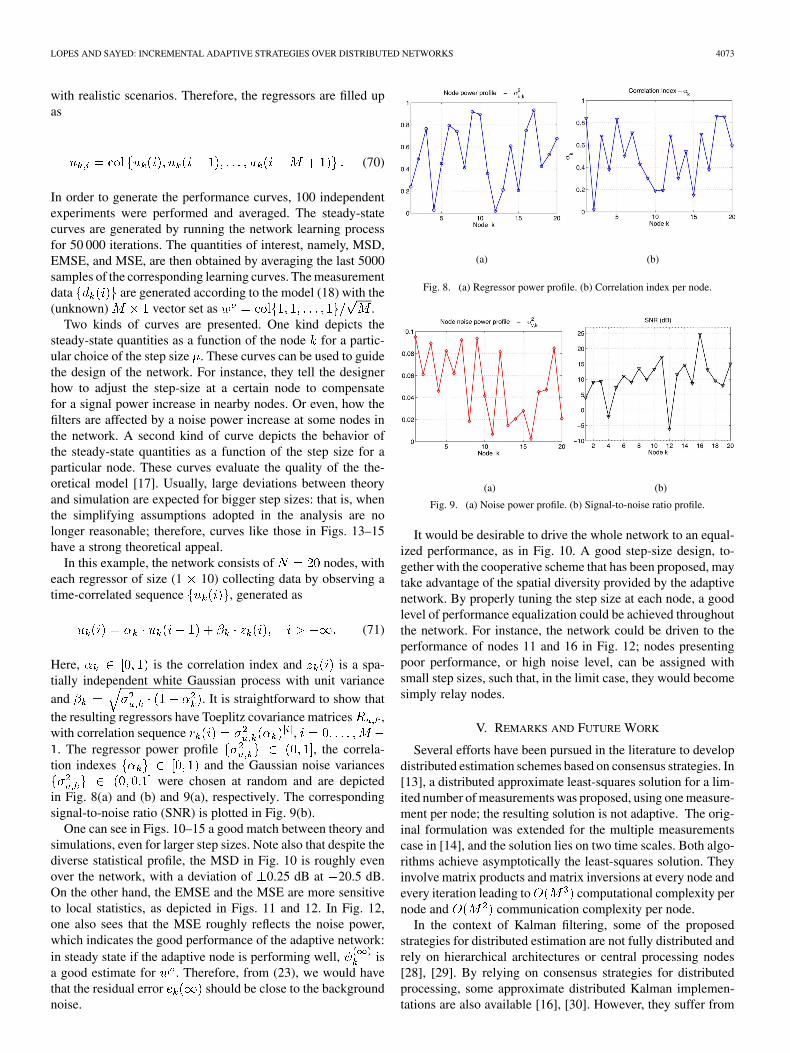
In this example, the network consists of nodes, witheach regressor of size (1 10) collecting data by observing atime-correlated sequence , generated as

(71)

Here, is the correlation index and is a spa-tially independent white Gaussian process with unit varianceand . It is straightforward to show thatthe resulting regressors have Toeplitz covariance matrices ,with correlation sequence ,

. The regressor power profile , the correla-tion indexes and the Gaussian noise variances

were chosen at random and are depictedin Fig. 8(a) and (b) and 9(a), respectively. The correspondingsignal-to-noise ratio (SNR) is plotted in Fig. 9(b).

One can see in Figs. 10–15 a good match between theory andsimulations, even for larger step sizes. Note also that despite thediverse statistical profile, the MSD in Fig. 10 is roughly evenover the network, with a deviation of 0.25 dB at 20.5 dB.On the other hand, the EMSE and the MSE are more sensitiveto local statistics, as depicted in Figs. 11 and 12. In Fig. 12,one also sees that the MSE roughly reflects the noise power,which indicates the good performance of the adaptive network:in steady state if the adaptive node is performing well, isa good estimate for . Therefore, from (23), we would havethat the residual error should be close to the backgroundnoise.

(a) (b)

Fig. 8. (a) Regressor power profile. (b) Correlation index per node.

(a) (b)

Fig. 9. (a) Noise power profile. (b) Signal-to-noise ratio profile.

It would be desirable to drive the whole network to an equal-ized performance, as in Fig. 10. A good step-size design, to-gether with the cooperative scheme that has been proposed, maytake advantage of the spatial diversity provided by the adaptivenetwork. By properly tuning the step size at each node, a goodlevel of performance equalization could be achieved throughoutthe network. For instance, the network could be driven to theperformance of nodes 11 and 16 in Fig. 12; nodes presentingpoor performance, or high noise level, can be assigned withsmall step sizes, such that, in the limit case, they would becomesimply relay nodes.

V. REMARKS AND FUTURE WORK

Several efforts have been pursued in the literature to developdistributed estimation schemes based on consensus strategies. In[13], a distributed approximate least-squares solution for a lim-ited number of measurements was proposed, using one measure-ment per node; the resulting solution is not adaptive. The orig-inal formulation was extended for the multiple measurementscase in [14], and the solution lies on two time scales. Both algo-rithms achieve asymptotically the least-squares solution. Theyinvolve matrix products and matrix inversions at every node andevery iteration leading to computational complexity pernode and communication complexity per node.

In the context of Kalman filtering, some of the proposedstrategies for distributed estimation are not fully distributed andrely on hierarchical architectures or central processing nodes[28], [29]. By relying on consensus strategies for distributedprocessing, some approximate distributed Kalman implemen-tations are also available [16], [30]. However, they suffer from


Fig. 10. MSD versus node—� = 0:03.

Fig. 11. EMSE versus node—� = 0:03.

Fig. 12. MSE versus node—� = 0:03.

limited response to fast changing processes when the commu-nication network has limited resources. Moreover, in Kalmanfilter implementations, one needs to model the process underobservation, e.g., as first-order Markov processes, as well as usedata statistics. Subsequently, the model has to be shared amongthe nodes in order to take advantage of the a priori knowledge.

In a more general vein, particle filters are more flexible interms of process modeling. They account for nonlinear modelsand non-Gaussian data through a set of filter candidates (or par-ticles) that try to approximate the process under observation.When properly designed, they may achieve accurate descrip-tions of the process of interest. However, as in Kalman filtering,

Fig. 13. MSD versus �—node 7.

Fig. 14. EMSE versus �—node 7.

particle filters require a priori knowledge about the process, rep-resented by probability distributions that are assumed known.They are also computationally complex and challenging to im-plement in a distributed manner. In [31], distributed particlefilters that rely on ring, or “chain,” topologies (trees are alsopossible) are proposed under certain conditions on the proba-bility distributions of the process. The resulting algorithms aredemanding in terms of computational complexity and commu-nication resources, thus limiting the ability of the network torespond efficiently to fast changing environments.

The results developed in this paper lead to good perfor-mance allied with low communication and computationalrequirements. The proposed distributed scheme requiresoperations per iteration per node for both communications andcomputations. The scheme inherits the robustness of LMS im-plementations and promptly respond to new data. The solutiondoes not require two separate time scales. More sophisticatedcooperative modes (rather than the incremental mode) can alsobe pursued, e.g., a diffusion mode of the form [15], [18]:

for a local combiner that consults nodes from theneighborhood . This additional level of complexityleads to more challenging and more interesting distributed


Fig. 15. MSE versus �—node 7.

adaptive structures that can still be examined and studied bythe tools and framework developed in this paper, albeit withmore effort. This work can also be extended to operate overthe collaboration protocols proposed in [32] and [33] and toother adaptive algorithms at the node level. We will extend thecurrent discussion to these more general scenarios in futureworks.

APPENDIX ACOMPARING STEEPEST-DESCENT AND

ITS INCREMENTAL VERSION

We want to compare algorithms (14) and (13) to provide in-sights about their stochastic counterparts. For simplicity, assumethat the statistical profile throughout the network is roughly sim-ilar, i.e., , and , such that (14)becomes

(72)

Subtracting both sides from and using (19) yields, or, equivalently

(73)

so that

Incremental (74)

where is the global weight error vector. Now,employing the eigendecomposition and definingthe transformed vector , we get

(75)

Similarly, for the steepest-descent algorithm (13), we have

(76)

so that and

Steepest-Descent (77)

Fig. 16. Modes of convergence for algorithms (13) and (14).

Writing (77) in terms of the transformed vector, we arrive at

(78)

From (75) and (78), we find that the modes of convergenceof the algorithms are given by

(79)

for . Fig. 16 shows both modes of convergencefor the case , where is the normalized stepsize. Note that for larger step sizes, the incremental algorithmhas a faster convergence rate than the steepest-descent solution.The incremental algorithm has a fast convergence rate even forsmall step sizes, which supports why its corresponding incre-mental adaptive version has better convergence rate togetherwith a smaller MSE in steady state. Furthermore, the stabilityrange for the incremental algorithm is wider, leading to morerobust implementations.

As a matter of fact, for diminishing step sizes, the incrementalsolution (14) and the steepest-descent solution (13) tend to thesame behavior also with diverse statistical profiles over the net-work. To observe this fact, we first note from (9) that thepartial gradient is given by

(80)

Inspecting (80), we note that the following equality holds for ascalar and any two column vectors and :

(81)

where is computed relative to . Now, we iterate the in-cremental solution (14) starting with , as follows:

...

(82)


Fig. 17. Plot of ratio � (i) at node 1 for algorithms (16) and (17).

Substituting (82) into the argument of in (14) gives

(83)

Using relation (81) with the choices andleads to

(84)

Therefore, the incremental algorithm can be written as a sum ofthe steepest-descent update plus extra terms. As , theterm dominates the term, and the incremental algorithm (14)and the standard gradient (13) tend to the same behavior. Theratio

(85)

is plotted in Fig. 17 for the incremental adaptive solution (16)and the stochastic steepest-descent (17), both at node 1. Thesame settings as the example presented in Figs. 6 and 7 are used,and 200 experiments are run, with throughout thenetwork. As , both algorithms exhibit similar behavior,as suggested by (84).

ACKNOWLEDGMENT

The authors would like to acknowledge the contribution ofthe graduate student F. Cattivelli to some of the arguments inAppendix A.

REFERENCES

[1] D. Estrin, G. Pottie, and M. Srivastava, “Intrumenting the world withwireless sensor setworks,” in Proc. IEEE Int. Conf. Acoustics, Speech,Signal Processing (ICASSP), Salt Lake City, UT, May 2001, pp.2033–2036.

[2] M. G. Rabbat and R. D. Nowak, “Quantized incremental algorithms fordistributed optimization,” IEEE J. Sel. Areas Commun., vol. 23, no. 4,pp. 798–808, Apr. 2005.

[3] M. Wax and T. Kailath, “Decentralized processing in sensor arrays,”IEEE Trans. Acoust., Speech, Signal Process., vol. ASSP-33, no. 4, pp.1123–1129, Oct. 1985.

[4] J. Tsitsiklis and M. Athans, “Convergence and asymptotic agreementin distributed decision problems,” IEEE Trans. Autom. Control, vol.AC-29, no. 1, pp. 42–50, Jan. 1984.

[5] R. Olfati-Saber and R. M. Murray, “Consensus problems in networks ofagents with switching topology and time-delays,” IEEE Trans. Autom.Control, vol. 49, no. 9, pp. 1520–1533, Sep. 2004.

[6] L. Xiao and S. Boyd, “Fast linear iterations for distributed averaging,”Syst. Control Lett., vol. 53, no. 1, pp. 65–78, Sep. 2004.

[7] L. A. Rossi, B. Krishnamachari, and C.-C. J. Kuo, “Distributedparameter estimation for monitoring diffusion phenomena usingphysical models,” in Proc. 1st IEEE Conf. Sensor and Ad HocCommunications and Networks, Santa Clara, CA, Oct. 2004, pp.460–469.

[8] D. Li, K. D. Wong, Y. H. Hu, and A. M. Sayeed, “Detection, classi-fication, and tracking of targets,” IEEE Signal Process. Mag., vol. 19,no. 2, pp. 17–29, Mar. 2002.

[9] I. Akyildiz, W. Su, Y. Sankarasubramaniam, and E. Cayirci, “A surveyon sensor networks,” IEEE Commun. Mag., vol. 40, no. 8, pp. 102–114,Aug. 2002.

[10] D. Culler, D. Estrin, and M. Srivastava, “Overview of sensor networks,”Computer, vol. 37, no. 8, pp. 41–49, Aug. 2004.

[11] M. G. Rabbat and R. D. Nowak, “Decentralized source localizationand tracking,” in Proc. IEEE Int. Conf. Acoustics, Speech, SignalProcessing (ICASSP), Montreal, QC, Canada, May 2004, vol. III, pp.921–924.

[12] C. G. Lopes and A. H. Sayed, “Distributed adaptive incrementalstrategies: Formulation and performance analysis,” in Proc. IEEEInt. Conf. Acoustics, Speech, Signal Processing (ICASSP), Toulouse,France, May 2006, vol. 3, pp. 584–587.

[13] L. Xiao, S. Boyd, and S. Lall, “A scheme for robust distributed sensorfusion based on average consensus,” in Proc. 4th Int. Symp. Informa-tion Processing in Sensor Networks, Los Angeles, CA, Apr. 2005, pp.63–70.

[14] L. Xiao, S. Boyd, and S. Lall, “A space-time diffusion schemefor peer-to-peer least-squares estimation,” in Proc. 5th Int. Symp.Information Processing in Sensor Networks, Nashville, TN, Apr.2006.

[15] C. G. Lopes and A. H. Sayed, “Diffusion least-mean squares over adap-tive networks,” in Proc. IEEE Int. Conf. Acoustics, Speech, Signal Pro-cessing (ICASSP), Honolulu, HI, Apr. 2007, pp. 917–920.

[16] D. P. Spanos, R. Olfati-Saber, and R. M. Murray, “Approximate dis-tributed Kalman filtering in sensor networks with quantifiable perfor-mance,” in Proc. 4th Int. Symp. Information Processing in Sensor Net-works, Los Angeles, CA, Apr. 2005, pp. 133–139.

[17] A. H. Sayed, Fundamentals of Adaptive Filtering. New York: Wiley,2003.

[18] C. G. Lopes and A. H. Sayed, “Distributed processing over adaptivenetworks,” in Proc. Adaptive Sensor Array Processing Workshop, MITLincoln Lab., Lexington, MA, Jun. 2006.

[19] A. H. Sayed and C. G. Lopes, “Distributed recursive least-squaresstrategies over adaptive networks,” in Proc. Asilomar Conf. Signals,Systems, Computers, Monterey, CA, Oct. 2006, pp. 233–237.

[20] D. Bertsekas, “A new class of incremental gradient methods for leastsquares problems,” SIAM J. Optim., vol. 7, no. 4, pp. 913–926, Nov.1997.

[21] A. Nedic and D. Bertsekas, “Incremental subgradient methods fornondifferentiable optimization,” SIAM J. Optim., vol. 12, no. 1, pp.109–138, 2001.

[22] J. Tsitsiklis, D. P. Bertsekas, and M. Athans, “Distributed asyn-chronous deterministic and stochastic gradient optimization algo-rithms,” IEEE Trans. Autom. Control, vol. AC-31, no. 9, pp. 650–655,Sep. 1986.

[23] B. T. Poljak and Y. Z. Tsypkin, “Pseudogradient adaptation andtraining algorithms,” Autom. Remote Control, vol. 12, pp. 83–94,1973.


[24] J. Haupt and R. Nowak, “Signal reconstruction from randomized pro-jections with applications to wireless sensing,” in Proc. 13th Work-shop on Statistical Signal Processing, Bordeaux, France, Jul. 2005, pp.1182–1187.

[25] H. Benali, M. Pelegrini, and F. Kruggel, “Spatio-temporal covariancemodel for medical images sequences: Application to functional MRIdata,” in Information Processing in Medical Imaging, ser. LectureNotes in Computer Science. Berlin: Springer, 2001, vol. 2082, pp.197–203.

[26] N. R. Yousef and A. H. Sayed, “A unified approach to the steady-stateand tracking analyses of adaptive filters,” IEEE Trans. Signal Process.,vol. 49, no. 2, pp. 314–324, Feb. 2001.

[27] T. Y. A. Naffouri and A. H. Sayed, “Transient analysis of data-normal-ized adaptive filters,” IEEE Trans. Signal Process., vol. 51, no. 3, pp.639–652, Mar. 2003.

[28] S. C. Felter, “An overview of decentralized Kalman filter techniques,”in Proc. IEEE Southern Tier Technical Conf., Binghamton, NY, Apr.1990, pp. 79–87.

[29] L. Hong, “Adaptive distributed filtering in multicoordinated systems,”IEEE Trans. Aerosp. Electron. Syst., vol. 27, no. 4, pp. 715–724, Jul.1991.

[30] D. Spanos, R. Olfati-Saber, and R. Murray, “Distributed sensor fusionusing dynamic consensus,” presented at the 16th IFAC World Congr.,Prague, Czech Republic, Jul. 2005.

[31] M. Coates, “Distributed particle filters for sensor networks,” in Proc.3rd Int. Symp. Information Processing in Sensor Networks, Apr. 2004,pp. 99–107.

[32] C. E. Guestrin, P. Bodik, R. Thibaux, M. A. Paskin, and S. Madden,“Distributed regression: An efficient framework for modeling sensornetwork data,” in Proc. 3rd Int. Symp. Information Processing in SensorNetworks, Berkeley, CA, Apr. 2004, pp. 1–10.

[33] M. A. Paskin, C. E. Guestrin, and J. McFadden, “A robust architec-ture for inference in sensor networks,” in Proc. 4th Int. Symp. Informa-tion Processing in Sensor Networks, Los Angeles, CA, Apr. 2005, pp.55–62.

Cassio G. Lopes (S’06) received the B.S. degree andthe M.S. degree in electrical engineering from theFederal University of Santa Catarina, Brazil, in 1997and 1999, respectively, and the M.S. degree in elec-trical engineering from the University of California,Los Angeles (UCLA) in 2004, where he is currentlypursuing the Ph.D. degree in electrical engineeringat the UCLA Adaptive Systems Laboratory, in dis-tributed adaptive estimation.

From 1999 to 2002, he worked with hardware de-sign for biomedical signals acquisition and transmis-

sion over the Internet. He also taught undergraduate-level courses in computerscience and electrical engineering. Since 2005, he has been working at the Adap-tive Systems Lab/UCLA as a Researcher Staff to develop efficient frequencyestimation algorithms for direct-to-earth Mars communications, in cooperationwith the Jet Propulsion Lab/NASA. His current research interests are theory andmethods for adaptive and statistical signal processing, distributed adaptive esti-mation, as well as frequency estimation algorithms for space communications.

Ali H. Sayed (S’90–M’92–SM’99–F’01) receivedthe Ph.D. degree in electrical engineering fromStanford University, Stanford, CA, in 1992.

He is Professor and Chairman of Electrical Engi-neering with the University of California, Los An-geles (UCLA). He is also the Principal Investigatorof the UCLA Adaptive Systems Laboratory (http://www.ee.ucla.edu/asl). He has more than 280 journaland conference publications. He is the author of Fun-damentals of Adaptive Filtering (New York: Wiley,2003), coauthor of the research monograph Indefi-

nite Quadratic Estimation and Control (Philadelphia, PA: SIAM, 1999) andof the graduate-level textbook Linear Estimation (Englewood Cliffs, NJ: Pren-tice-Hall, 2000). He is also coeditor of the volume Fast Reliable Algorithms forMatrices with Structure (Philadelphia, PA: SIAM, 1999). He has contributedseveral articles to engineering and mathematical encyclopedias and handbooksand has served on the program committees of several international meetings.His research interests span several areas, including adaptive and statistical signalprocessing, filtering and estimation theories, signal processing for communica-tions, interplays between signal processing and control methodologies, systemtheory, and fast algorithms for large-scale problems.

Dr. Sayed received the 1996 IEEE Donald G. Fink Award, 2002 Best PaperAward from the IEEE Signal Processing Society, 2003 Kuwait Prize in BasicScience, 2005 Frederick E. Terman Award, and is coauthor of two Best StudentPaper awards at international meetings (1999, 2001). He is also a member ofthe Technical Committees on Signal Processing Theory and Methods (SPTM)and on Signal Processing for Communications (SPCOM), both of the IEEESignal Processing Society. He is a member of the editorial board of the IEEESignal Processing Magazine. He has also served twice as an Associate Editorof the IEEE TRANSACTIONS ON SIGNAL PROCESSING, and as Editor-in-Chiefof the same journal during 2003-2005. He is serving as Editor-in-Chief of theEURASIP Journal on Advances in Signal Processing and as General Chairmanof IEEE International Conference on Acoustics, Speech and Signal Processing(ICASSP) 2008. He sits on the Board of Governors of the IEEE Signal Pro-cessing Society.

Incremental Adaptive Strategies Over Distributed Networks

Documents

Transcript of Incremental Adaptive Strategies Over Distributed Networks