On simplifying ‘incremental remap’-based transport schemes

Peter H. Lauritzena,!, Christoph Erathb, Rashmi Mittalc

aClimate and Global Dynamics Division, National Center for Atmospheric Research, P.O. Box 3000, Boulder, CO80307, USA

bThe Computational & Information Systems Laboratory, National Center for Atmospheric Research, P.O. Box 3000,Boulder, CO 80307, USA

cMesoscale and Microscale Meteorology Division, National Center for Atmospheric Research, P.O. Box 3000, Boulder,CO 80307-3000

AbstractThe flux-form incremental remapping transport scheme introduced by Dukowicz and Baum-gardner [1] converts the transport problem into a remapping problem. This involves identifyingoverlap areas between quadrilateral flux-areas and regular square grid cells which is non-trivialand leads to some algorithm complexity. In the simpler swept area approach (originally intro-duced by Hirt et al. [2]) the search for overlap areas is eliminated even if the flux-areas overlapseveral regular grid cells. The resulting simplified scheme leads to a much simpler and robustalgorithm.

We show that for su!ciently small Courant numbers (approximatelyCFL"1/2) the simplified(or swept area) scheme can be more accurate than the original incremental remapping scheme.This is demonstrated through a Von Neumann stability analysis, an error analysis and in idealizedtransport test cases on the sphere using the ‘incremental remapping’-based scheme called FF-CSLAM (Flux-Form version of the Conservative Semi-Lagrangian Multi-tracer scheme) on thecubed-sphere.

Keywords: Conservative Transport, Cubed-sphere, Error Analysis, Finite-Volume, Flux-FormSemi-Lagrangian, Von Neumann Stability Analysis, Remapping, Multi-Tracer Transport

1. Introduction

Consider the flux-form continuity equation for some inert and passive mass variable ! (forexample, fluid density " or tracer density " q, where q is a mixing ratio)

#!

#t+ # · !!$v" = 0, (1)

where $v = (u, v) is the velocity vector. Following [1], the 2D Cartesian discretization of theintegral form of (1) for a particular grid cell A can be written as

#!n+1 $ !n

$|A| $ (FW + FS + FE + FN) = 0, (2)

!Corresponding author. Tel.: +1 303 497 1316; fax: +1 303 497 1324.Email address: pel@ucar.edu (Peter H. Lauritzen)URL: http://www.cgd.ucar.edu/cms/pel/ (Peter H. Lauritzen)1The National Center for Atmospheric Research is sponsored by the National Science Foundation.

Preprint submitted to Journal of Computational Physics June 2, 2011

A1

A2 A3

A4

AW AE

$v

µx"x"x

µy"y

"y

(0, 0)

(a) West and east cell edge.

A1

A2 A3

A4

AS

AN

$v

µx"x"x

µy"y

"y

(0, 0)

(b) North and south cell edge.

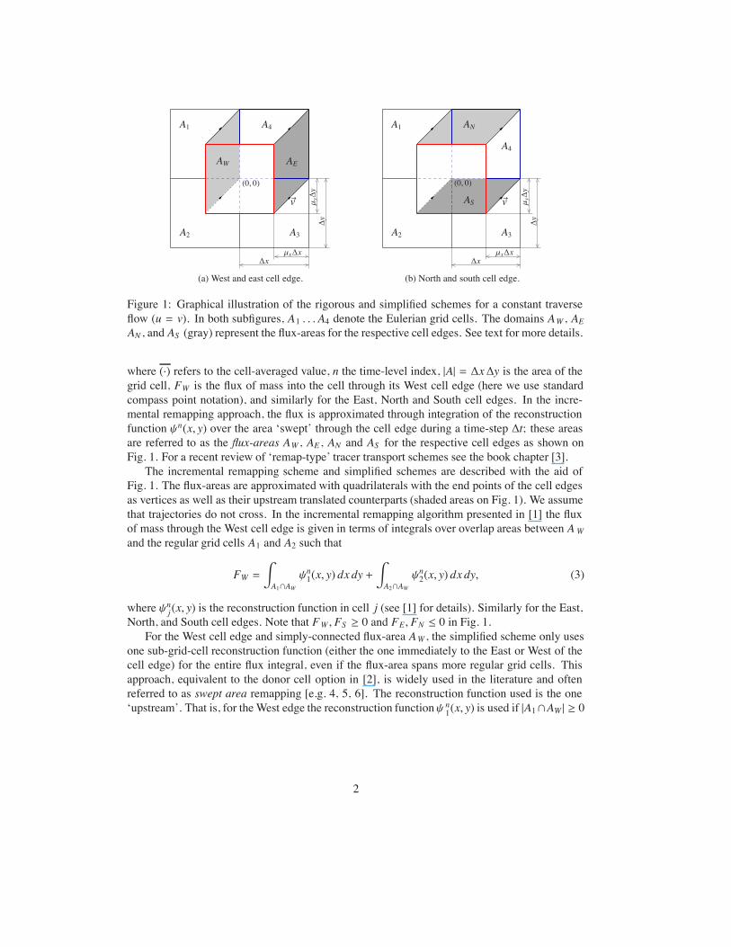
Figure 1: Graphical illustration of the rigorous and simplified schemes for a constant traverseflow (u = v). In both subfigures, A1 . . . A4 denote the Eulerian grid cells. The domains AW , AEAN , and AS (gray) represent the flux-areas for the respective cell edges. See text for more details.

where (·) refers to the cell-averaged value, n the time-level index, |A| = "x"y is the area of thegrid cell, FW is the flux of mass into the cell through its West cell edge (here we use standardcompass point notation), and similarly for the East, North and South cell edges. In the incre-mental remapping approach, the flux is approximated through integration of the reconstructionfunction !n(x, y) over the area ‘swept’ through the cell edge during a time-step "t; these areasare referred to as the flux-areas AW , AE , AN and AS for the respective cell edges as shown onFig. 1. For a recent review of ‘remap-type’ tracer transport schemes see the book chapter [3].

The incremental remapping scheme and simplified schemes are described with the aid ofFig. 1. The flux-areas are approximated with quadrilaterals with the end points of the cell edgesas vertices as well as their upstream translated counterparts (shaded areas on Fig. 1). We assumethat trajectories do not cross. In the incremental remapping algorithm presented in [1] the fluxof mass through the West cell edge is given in terms of integrals over overlap areas between AWand the regular grid cells A1 and A2 such that

FW =%

A1%AW!n1(x, y) dx dy +

%

A2%AW!n2(x, y) dx dy, (3)

where !nj (x, y) is the reconstruction function in cell j (see [1] for details). Similarly for the East,North, and South cell edges. Note that FW , FS & 0 and FE , FN " 0 in Fig. 1.

For the West cell edge and simply-connected flux-area AW , the simplified scheme only usesone sub-grid-cell reconstruction function (either the one immediately to the East or West of thecell edge) for the entire flux integral, even if the flux-area spans more regular grid cells. Thisapproach, equivalent to the donor cell option in [2], is widely used in the literature and oftenreferred to as swept area remapping [e.g. 4, 5, 6]. The reconstruction function used is the one‘upstream’. That is, for theWest edge the reconstruction function! n1(x, y) is used if |A1%AW | & 0

2

N1

N2

µ"x

µ"x

AN,1AN,2"x/2

"x

A1

A2 A3

A4

(0, 0)

(a) ‘Anti clockwise’ hourglass movementof the North edge.

N1

N2

µ"x

µ"x

AN,1

AN,2"x/2

"x

A1

A2 A3

A4

(0, 0)

(b) ‘Clockwise’ hourglass movement ofthe North edge.

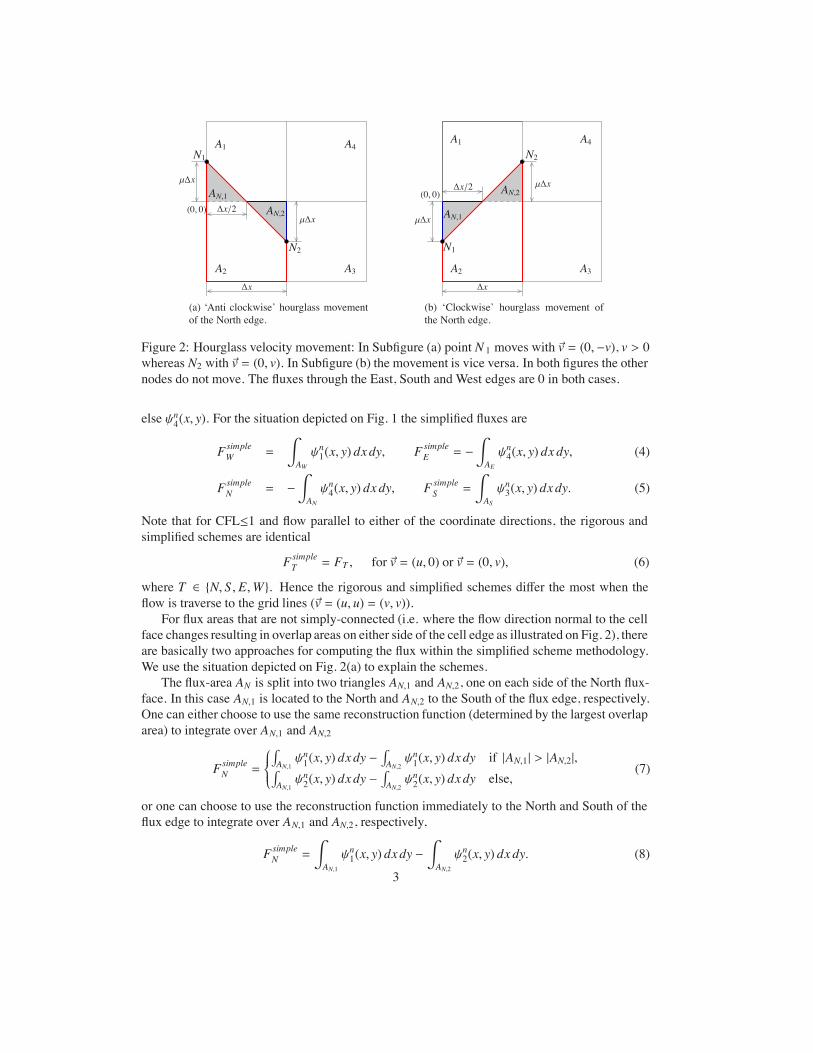
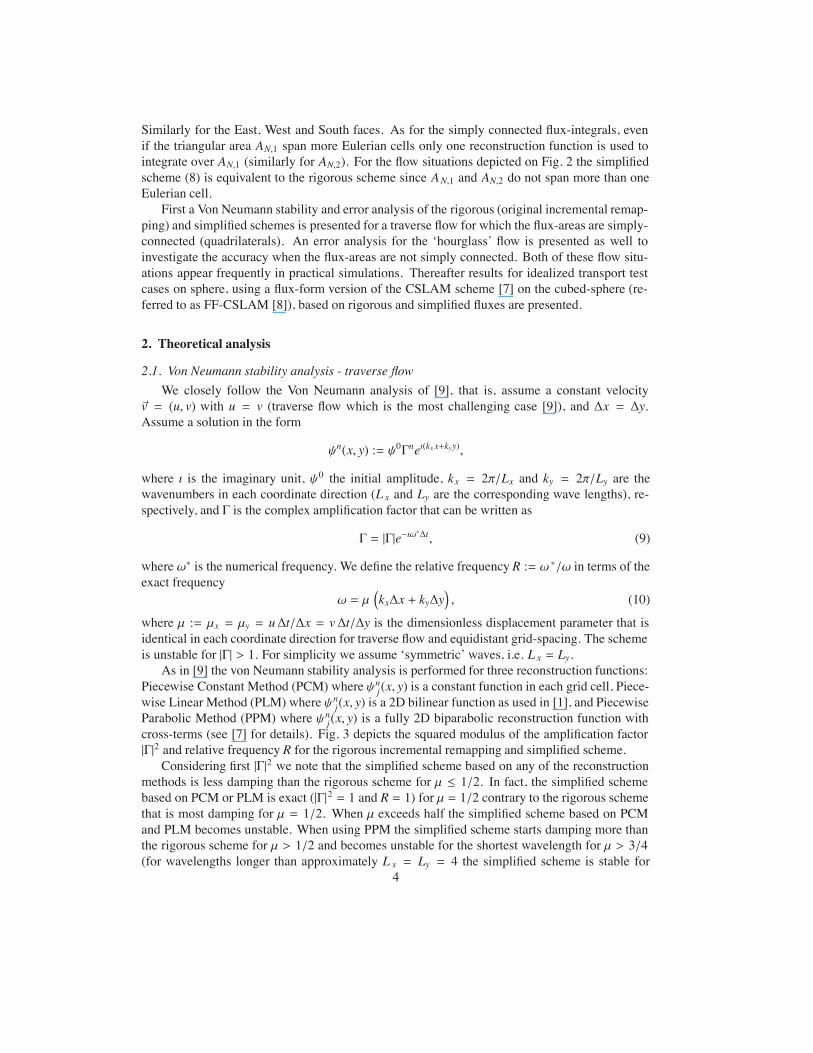
Figure 2: Hourglass velocity movement: In Subfigure (a) point N 1 moves with $v = (0,$v), v > 0whereas N2 with $v = (0, v). In Subfigure (b) the movement is vice versa. In both figures the othernodes do not move. The fluxes through the East, South and West edges are 0 in both cases.

else !n4(x, y). For the situation depicted on Fig. 1 the simplified fluxes are

FsimpleW =

%

AW!n1(x, y) dxdy, Fsimple

E = $%

AE!n4(x, y) dx dy, (4)

FsimpleN = $

%

AN!n4(x, y) dx dy, Fsimple

S =

%

AS!n3(x, y) dxdy. (5)

Note that for CFL"1 and flow parallel to either of the coordinate directions, the rigorous andsimplified schemes are identical

FsimpleT = FT , for $v = (u, 0) or $v = (0, v), (6)

where T ' {N, S , E,W}. Hence the rigorous and simplified schemes di#er the most when theflow is traverse to the grid lines ($v = (u, u) = (v, v)).

For flux areas that are not simply-connected (i.e. where the flow direction normal to the cellface changes resulting in overlap areas on either side of the cell edge as illustrated on Fig. 2), thereare basically two approaches for computing the flux within the simplified scheme methodology.We use the situation depicted on Fig. 2(a) to explain the schemes.

The flux-area AN is split into two triangles AN,1 and AN,2, one on each side of the North flux-face. In this case AN,1 is located to the North and AN,2 to the South of the flux edge, respectively.One can either choose to use the same reconstruction function (determined by the largest overlaparea) to integrate over AN,1 and AN,2

FsimpleN =

&''('')

*AN,1!n1(x, y) dxdy $

*AN,2!n1(x, y) dxdy if |AN,1| > |AN,2|,*

AN,1!n2(x, y) dxdy $

*AN,2!n2(x, y) dxdy else,

(7)

or one can choose to use the reconstruction function immediately to the North and South of theflux edge to integrate over AN,1 and AN,2, respectively,

FsimpleN =

%

AN,1!n1(x, y) dxdy $

%

AN,2!n2(x, y) dx dy. (8)

3

Similarly for the East, West and South faces. As for the simply connected flux-integrals, evenif the triangular area AN,1 span more Eulerian cells only one reconstruction function is used tointegrate over AN,1 (similarly for AN,2). For the flow situations depicted on Fig. 2 the simplifiedscheme (8) is equivalent to the rigorous scheme since AN,1 and AN,2 do not span more than oneEulerian cell.

First a Von Neumann stability and error analysis of the rigorous (original incremental remap-ping) and simplified schemes is presented for a traverse flow for which the flux-areas are simply-connected (quadrilaterals). An error analysis for the ‘hourglass’ flow is presented as well toinvestigate the accuracy when the flux-areas are not simply connected. Both of these flow situ-ations appear frequently in practical simulations. Thereafter results for idealized transport testcases on sphere, using a flux-form version of the CSLAM scheme [7] on the cubed-sphere (re-ferred to as FF-CSLAM [8]), based on rigorous and simplified fluxes are presented.

2. Theoretical analysis

2.1. Von Neumann stability analysis - traverse flowWe closely follow the Von Neumann analysis of [9], that is, assume a constant velocity

$v = (u, v) with u = v (traverse flow which is the most challenging case [9]), and "x = "y.Assume a solution in the form

!n(x, y) := !0$neı(kx x+kyy),

where ı is the imaginary unit, !0 the initial amplitude, kx = 2%/Lx and ky = 2%/Ly are thewavenumbers in each coordinate direction (L x and Ly are the corresponding wave lengths), re-spectively, and $ is the complex amplification factor that can be written as

$ = |$|e$ı&!"t, (9)

where &! is the numerical frequency. We define the relative frequency R := & !/& in terms of theexact frequency

& = µ+kx"x + ky"y

,, (10)

where µ := µx = µy = u"t/"x = v"t/"y is the dimensionless displacement parameter that isidentical in each coordinate direction for traverse flow and equidistant grid-spacing. The schemeis unstable for |$| > 1. For simplicity we assume ‘symmetric’ waves, i.e. L x = Ly.

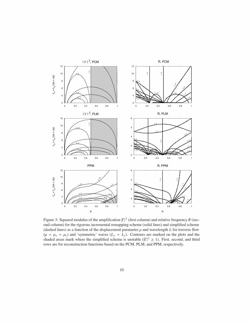
As in [9] the von Neumann stability analysis is performed for three reconstruction functions:Piecewise Constant Method (PCM) where !nj (x, y) is a constant function in each grid cell, Piece-wise Linear Method (PLM) where !nj(x, y) is a 2D bilinear function as used in [1], and PiecewiseParabolic Method (PPM) where !nj(x, y) is a fully 2D biparabolic reconstruction function withcross-terms (see [7] for details). Fig. 3 depicts the squared modulus of the amplification factor|$|2 and relative frequency R for the rigorous incremental remapping and simplified scheme.

Considering first |$|2 we note that the simplified scheme based on any of the reconstructionmethods is less damping than the rigorous scheme for µ " 1/2. In fact, the simplified schemebased on PCM or PLM is exact (|$|2 = 1 and R = 1) for µ = 1/2 contrary to the rigorous schemethat is most damping for µ = 1/2. When µ exceeds half the simplified scheme based on PCMand PLM becomes unstable. When using PPM the simplified scheme starts damping more thanthe rigorous scheme for µ > 1/2 and becomes unstable for the shortest wavelength for µ > 3/4(for wavelengths longer than approximately L x = Ly = 4 the simplified scheme is stable for

4

Courant numbers exceeding one). The simplified scheme most likely becomes unstable becausethe region of ‘extrapolation’ (overlap between flux-area and non-adjacent upstream grid cell, e.g.,A2 % AW for AW ) becomes too large compared to the flux-overlap-area adjacent and upstream tothe cell edge (e.g., A1 % AW). Similar observations are made for the relative frequency R.

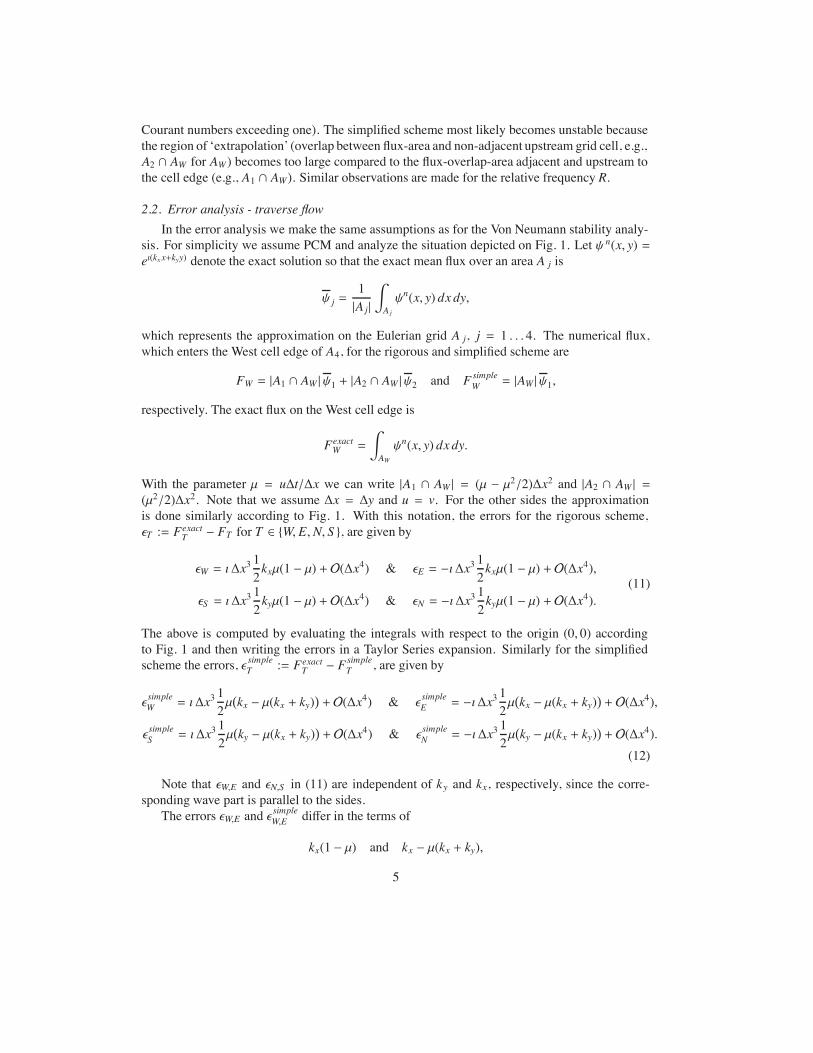
2.2. Error analysis - traverse flowIn the error analysis we make the same assumptions as for the Von Neumann stability analy-

sis. For simplicity we assume PCM and analyze the situation depicted on Fig. 1. Let ! n(x, y) =eı(kx x+kyy) denote the exact solution so that the exact mean flux over an area A j is

! j =1|Aj|

%

Aj

!n(x, y) dx dy,

which represents the approximation on the Eulerian grid A j, j = 1 . . .4. The numerical flux,which enters the West cell edge of A4, for the rigorous and simplified scheme are

FW = |A1 % AW |!1 + |A2 % AW |!2 and FsimpleW = |AW |!1,

respectively. The exact flux on the West cell edge is

FexactW =

%

AW!n(x, y) dx dy.

With the parameter µ = u"t/"x we can write |A1 % AW | = (µ $ µ2/2)"x2 and |A2 % AW | =(µ2/2)"x2. Note that we assume "x = "y and u = v. For the other sides the approximationis done similarly according to Fig. 1. With this notation, the errors for the rigorous scheme,'T := FexactT $ FT for T ' {W, E,N, S }, are given by

'W = ı"x312kxµ(1 $ µ) + O("x4) & 'E = $ı"x3

12kxµ(1 $ µ) + O("x4),

'S = ı"x312kyµ(1 $ µ) + O("x4) & 'N = $ı"x3

12kyµ(1 $ µ) + O("x4).

(11)

The above is computed by evaluating the integrals with respect to the origin (0, 0) accordingto Fig. 1 and then writing the errors in a Taylor Series expansion. Similarly for the simplifiedscheme the errors, ' simpleT := FexactT $ Fsimple

T , are given by

' simpleW = ı"x312µ!kx $ µ(kx + ky)

"+ O("x4) & ' simpleE = $ı"x3 12µ

!kx $ µ(kx + ky)

"+ O("x4),

' simpleS = ı"x312µ!ky $ µ(kx + ky)

"+ O("x4) & ' simpleN = $ı"x3 1

2µ!ky $ µ(kx + ky)

"+ O("x4).

(12)

Note that 'W,E and 'N,S in (11) are independent of ky and kx, respectively, since the corre-sponding wave part is parallel to the sides.

The errors 'W,E and ' simpleW,E di#er in the terms of

kx(1 $ µ) and kx $ µ(kx + ky),

5

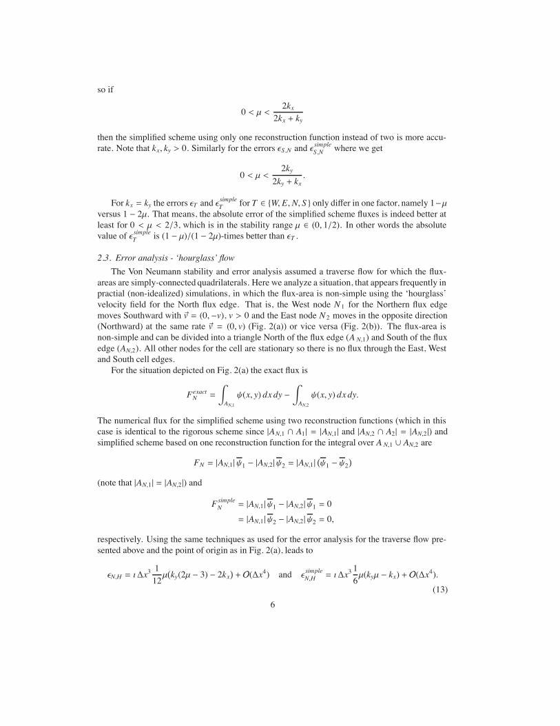
so if

0 < µ < 2kx2kx + ky

then the simplified scheme using only one reconstruction function instead of two is more accu-rate. Note that kx, ky > 0. Similarly for the errors 'S ,N and ' simpleS ,N where we get

0 < µ <2ky

2ky + kx.

For kx = ky the errors 'T and ' simpleT for T ' {W, E,N, S } only di#er in one factor, namely 1$µversus 1 $ 2µ. That means, the absolute error of the simplified scheme fluxes is indeed better atleast for 0 < µ < 2/3, which is in the stability range µ ' (0, 1/2). In other words the absolutevalue of ' simpleT is (1 $ µ)/(1 $ 2µ)-times better than 'T .

2.3. Error analysis - ‘hourglass’ flowThe Von Neumann stability and error analysis assumed a traverse flow for which the flux-

areas are simply-connected quadrilaterals. Here we analyze a situation, that appears frequently inpractial (non-idealized) simulations, in which the flux-area is non-simple using the ‘hourglass’velocity field for the North flux edge. That is, the West node N 1 for the Northern flux edgemoves Southward with $v = (0,$v), v > 0 and the East node N 2 moves in the opposite direction(Northward) at the same rate $v = (0, v) (Fig. 2(a)) or vice versa (Fig. 2(b)). The flux-area isnon-simple and can be divided into a triangle North of the flux edge (A N,1) and South of the fluxedge (AN,2). All other nodes for the cell are stationary so there is no flux through the East, Westand South cell edges.

For the situation depicted on Fig. 2(a) the exact flux is

FexactN =

%

AN,1!(x, y) dx dy $

%

AN,2!(x, y) dx dy.

The numerical flux for the simplified scheme using two reconstruction functions (which in thiscase is identical to the rigorous scheme since |AN,1 % A1| = |AN,1| and |AN,2 % A2| = |AN,2|) andsimplified scheme based on one reconstruction function for the integral over A N,1 ( AN,2 are

FN = |AN,1|!1 $ |AN,2|!2 = |AN,1|!!1 $ !2

"

(note that |AN,1| = |AN,2|) and

FsimpleN = |AN,1|!1 $ |AN,2|!1 = 0

= |AN,1|!2 $ |AN,2|!2 = 0,

respectively. Using the same techniques as used for the error analysis for the traverse flow pre-sented above and the point of origin as in Fig. 2(a), leads to

'N,H = ı"x3112µ!ky(2µ $ 3) $ 2kx

"+ O("x4) and ' simpleN,H = ı"x3

16µ(kyµ $ kx) + O("x4).

(13)6

The errors 'N,H and ' simpleN,H di#er in the terms of

ky-µ $ 3

2

.$ kx and kyµ $ kx,

so if

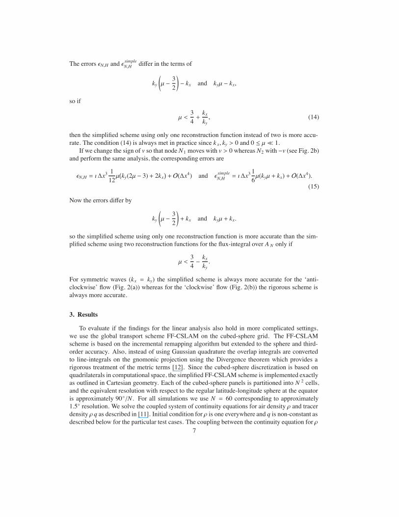
µ <34+kxky, (14)

then the simplified scheme using only one reconstruction function instead of two is more accu-rate. The condition (14) is always met in practice since k x, ky > 0 and 0 " µ ) 1.

If we change the sign of v so that node N1 moves with v > 0 whereas N2 with $v (see Fig. 2b)and perform the same analysis, the corresponding errors are

'N,H = ı"x3112µ!ky(2µ $ 3) + 2kx

"+ O("x4) and ' simpleN,H = ı"x3

16µ(kyµ + kx) + O("x4).

(15)

Now the errors di#er by

ky-µ $ 3

2

.+ kx and kyµ + kx.

so the simplified scheme using only one reconstruction function is more accurate than the sim-plified scheme using two reconstruction functions for the flux-integral over A N only if

µ <34$ kxky.

For symmetric waves (kx = ky) the simplified scheme is always more accurate for the ‘anti-clockwise’ flow (Fig. 2(a)) whereas for the ‘clockwise’ flow (Fig. 2(b)) the rigorous scheme isalways more accurate.

3. Results

To evaluate if the findings for the linear analysis also hold in more complicated settings,we use the global transport scheme FF-CSLAM on the cubed-sphere grid. The FF-CSLAMscheme is based on the incremental remapping algorithm but extended to the sphere and third-order accuracy. Also, instead of using Gaussian quadrature the overlap integrals are convertedto line-integrals on the gnomonic projection using the Divergence theorem which provides arigorous treatment of the metric terms [12]. Since the cubed-sphere discretization is based onquadrilaterals in computational space, the simplified FF-CSLAM scheme is implemented exactlyas outlined in Cartesian geometry. Each of the cubed-sphere panels is partitioned into N 2 cells,and the equivalent resolution with respect to the regular latitude-longitude sphere at the equatoris approximately 90*/N. For all simulations we use N = 60 corresponding to approximately1.5* resolution. We solve the coupled system of continuity equations for air density " and tracerdensity " q as described in [11]. Initial condition for " is one everywhere and q is non-constant asdescribed below for the particular test cases. The coupling between the continuity equation for "

7

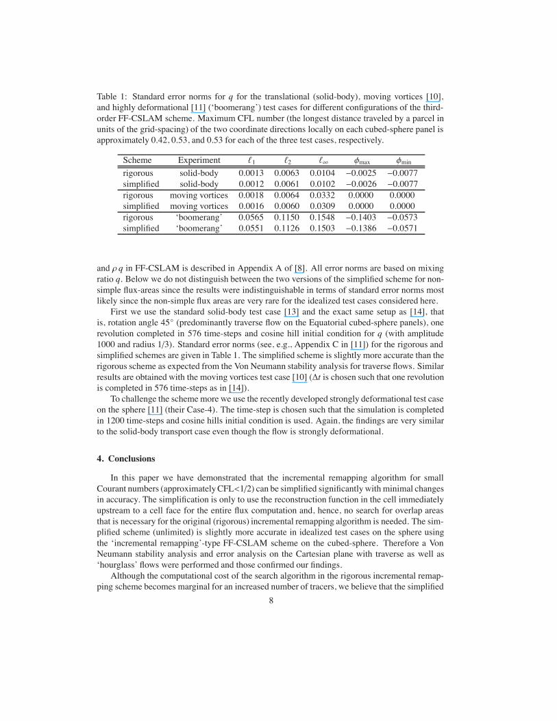
Table 1: Standard error norms for q for the translational (solid-body), moving vortices [10],and highly deformational [11] (‘boomerang’) test cases for di#erent configurations of the third-order FF-CSLAM scheme. Maximum CFL number (the longest distance traveled by a parcel inunits of the grid-spacing) of the two coordinate directions locally on each cubed-sphere panel isapproximately 0.42, 0.53, and 0.53 for each of the three test cases, respectively.

Scheme Experiment (1 (2 (+ )max )minrigorous solid-body 0.0013 0.0063 0.0104 $0.0025 $0.0077simplified solid-body 0.0012 0.0061 0.0102 $0.0026 $0.0077rigorous moving vortices 0.0018 0.0064 0.0332 0.0000 0.0000simplified moving vortices 0.0016 0.0060 0.0309 0.0000 0.0000rigorous ‘boomerang’ 0.0565 0.1150 0.1548 $0.1403 $0.0573simplified ‘boomerang’ 0.0551 0.1126 0.1503 $0.1386 $0.0571

and " q in FF-CSLAM is described in Appendix A of [8]. All error norms are based on mixingratio q. Below we do not distinguish between the two versions of the simplified scheme for non-simple flux-areas since the results were indistinguishable in terms of standard error norms mostlikely since the non-simple flux areas are very rare for the idealized test cases considered here.

First we use the standard solid-body test case [13] and the exact same setup as [14], thatis, rotation angle 45* (predominantly traverse flow on the Equatorial cubed-sphere panels), onerevolution completed in 576 time-steps and cosine hill initial condition for q (with amplitude1000 and radius 1/3). Standard error norms (see, e.g., Appendix C in [11]) for the rigorous andsimplified schemes are given in Table 1. The simplified scheme is slightly more accurate than therigorous scheme as expected from the Von Neumann stability analysis for traverse flows. Similarresults are obtained with the moving vortices test case [10] ("t is chosen such that one revolutionis completed in 576 time-steps as in [14]).

To challenge the schememore we use the recently developed strongly deformational test caseon the sphere [11] (their Case-4). The time-step is chosen such that the simulation is completedin 1200 time-steps and cosine hills initial condition is used. Again, the findings are very similarto the solid-body transport case even though the flow is strongly deformational.

4. Conclusions

In this paper we have demonstrated that the incremental remapping algorithm for smallCourant numbers (approximatelyCFL<1/2) can be simplified significantlywith minimal changesin accuracy. The simplification is only to use the reconstruction function in the cell immediatelyupstream to a cell face for the entire flux computation and, hence, no search for overlap areasthat is necessary for the original (rigorous) incremental remapping algorithm is needed. The sim-plified scheme (unlimited) is slightly more accurate in idealized test cases on the sphere usingthe ‘incremental remapping’-type FF-CSLAM scheme on the cubed-sphere. Therefore a VonNeumann stability analysis and error analysis on the Cartesian plane with traverse as well as‘hourglass’ flows were performed and those confirmed our findings.

Although the computational cost of the search algorithm in the rigorous incremental remap-ping scheme becomes marginal for an increased number of tracers, we believe that the simplified

8

scheme will render this flux-form semi-Lagrangian method more robust and computationallycompetitive even for a small number of tracers. For large Courant numbers, however, the rigor-ous scheme, e.g. FF-CSLAM, must be used.

Acknowledgements

The careful reviews by Dr. R.D.Nair (NCAR) and Dr. L.M. Harris (GFDL) are gratefullyacknowledged. The authors were partially supported by the DOEBER Program under award DE-SC0001658. We thank two anonymous reviewers for their helpful comments and suggestions thathave significantly improved this manuscript.

References

[1] J. K. Dukowicz, J. R. Baumgardner, Incremental remapping as a transport/advection algorithm, J. Comput. Phys.160 (2000) 318–335.

[2] C. W. Hirt, A. A. Amsden, J. L. Cook, An arbitrary Lagrangian-Eulerian computing method for all flow speeds, J.Comput. Phys. 14 (3) (1974) 227 – 253.

[3] P. H. Lauritzen, P. A. Ullrich, R. D. Nair, Atmospheric transport schemes: Desirable properties and a semi-Lagrangian view on finite-volume discretizations, Vol. 80 of Lecture Notes in Computational Science and En-gineering (Tutorials), Springer, 2011, Ch. 8, pp. 185–251.

[4] L. G. Margolin, M. Shashkov, Second-order sign-preserving conservative interpolation (remapping) on generalgrids, J. Comput. Phys. 184 (2003) 266–298.

[5] M. Kucharik, M. Shashkov, B. Wendro#, An e!cient linearity-and-bound-preserving remapping method, J. Com-put. Phys. 188 (2) (2003) 462 – 471.

[6] R. Loubere, M. J. Shashkov, A subcell remapping method on staggered polygonal grids for arbitrary-Lagrangian-Eulerian methods, J. Comput. Phys. 209 (1) (2005) 105 – 138.

[7] P. H. Lauritzen, R. D. Nair, P. A. Ullrich, A conservative semi-Lagrangian multi-tracer transport scheme (CSLAM)on the cubed-sphere grid, J. Comput. Phys. 229 (2010) 1401–1424.

[8] L. M. Harris, P. H. Lauritzen, R. Mittal, A flux-form version of the conservative semi-Lagrangian multi-tracertransport scheme (CSLAM) on the cubed sphere grid, J. Comput. Phys. 230 (4) (2010) 1215–1237.

[9] P. H. Lauritzen, A stability analysis of finite-volume advection schemes permitting long time steps, Mon. Wea. Rev.135 (2007) 2658–2673.

[10] R. D. Nair, C. Jablonowski, Moving vortices on the sphere: A test case for horizontal advection problems, Mon.Wea. Rev. 136 (2008) 699–711.

[11] R. D. Nair, P. H. Lauritzen, A class of deformational flow test cases for linear transport problems on the sphere, J.Comput. Phys. 229 (2010) 8868–8887.

[12] P. A. Ullrich, P. H. Lauritzen, C. Jablonowski, Geometrically exact conservative remapping (GECoRe): Regularlatitude-longitude and cubed-sphere grids., Mon. Wea. Rev. 137 (6) (2009) 1721–1741.

[13] D. L. Williamson, J. B. Drake, J. J. Hack, R. Jakob, P. N. Swarztrauber, A standard test set for numerical approxi-mations to the shallow water equations in spherical geometry, J. Comput. Phys. 102 (1992) 211–224.

[14] W. M. Putman, S.-J. Lin, Finite-volume transport on various cubed-sphere grids, J. Comput. Phys. 227 (1) (2007)55–78.

9

2

4

6

8

10

12

0 0.2 0.4 0.6 0.8 1

L x =

Ly (

x =

y)

| | 2, PCM

1.0

0.9

0.6

0.3

2

4

6

8

10

12

0 0.2 0.4 0.6 0.8 1

L x =

Ly (

x =

y)

| | 2, PLM

1.0

0.99

0.9

0.6

0.3

2

4

6

8

10

12

0 0.2 0.4 0.6 0.8 1

L x =

Ly (

x =

y)

µ

PPM

0.99

0.9

0.6

0.3

0.99

0.9

0.6

2

4

6

8

10

12

0 0.2 0.4 0.6 0.8 1

R, PCM

1.05

0.6

0.7

0.8

0.9

1.05

1.0

1.0

0.9

0.8

0.7

0.6

2

3

4

5

6

0 0.2 0.4 0.6 0.8 1

R, PLM

1.21.3

1.0

1.0

0.9

0.8

0.7

0.61.1

0.9

0.8

0.7

0.6

1.0

3

4

5

6

0 0.2 0.4 0.6 0.8 1

µ

R, PPM

1.4

1.3

1.2

1.2

1.1

1.0

1.0

0.9

0.8

0.7

0.6

Figure 3: Squared modulus of the amplification |$| 2 (first column) and relative frequency R (sec-ond column) for the rigorous incremental remapping scheme (solid lines) and simplified scheme(dashed lines) as a function of the displacement parameter µ and wavelength L for traverse flow(µ = µx = µy) and ‘symmetric’ waves (Lx = Ly). Contours are marked on the plots and theshaded areas mark where the simplified scheme is unstable (|$| 2 & 1). First, second, and thirdrows are for reconstruction functions based on the PCM, PLM, and PPM, respectively.

10