Efficient non-incremental constructive solid geometry evaluation for triangular meshes

Sheng, Bin; Li, Ping; Fu, Hongbo; Ma, Lizhuang; Wu, Enhua

Published in:Graphical Models

Published: 01/05/2018

Document Version:Post-print, also known as Accepted Author Manuscript, Peer-reviewed or Author Final version

License:CC BY-NC-ND

Publication record in CityU Scholars:Go to record

Published version (DOI):10.1016/j.gmod.2018.03.001

Publication details:Sheng, B., Li, P., Fu, H., Ma, L., & Wu, E. (2018). Efficient non-incremental constructive solid geometryevaluation for triangular meshes. Graphical Models, 97, 1-16. https://doi.org/10.1016/j.gmod.2018.03.001

Citing this paperPlease note that where the full-text provided on CityU Scholars is the Post-print version (also known as Accepted AuthorManuscript, Peer-reviewed or Author Final version), it may differ from the Final Published version. When citing, ensure thatyou check and use the publisher's definitive version for pagination and other details.

General rightsCopyright for the publications made accessible via the CityU Scholars portal is retained by the author(s) and/or othercopyright owners and it is a condition of accessing these publications that users recognise and abide by the legalrequirements associated with these rights. Users may not further distribute the material or use it for any profit-making activityor commercial gain.Publisher permissionPermission for previously published items are in accordance with publisher's copyright policies sourced from the SHERPARoMEO database. Links to full text versions (either Published or Post-print) are only available if corresponding publishersallow open access.

Take down policyContact lbscholars@cityu.edu.hk if you believe that this document breaches copyright and provide us with details. We willremove access to the work immediately and investigate your claim.

Download date: 27/01/2022

Efficient Non-incremental Constructive Solid GeometryEvaluation for Triangular Meshes

Bin Shenga,∗, Ping Lib,∗, Hongbo Fuc, Lizhuang Maa, Enhua Wud

aDepartment of Computer Science and Engineering, Shanghai Jiao Tong University, ChinabFaculty of Information Technology, Macau University of Science and Technology, Macau

cSchool of Creative Media, City University of Hong Kong, Hong KongdUniversity of Macau, and State Key Lab. of CS, ISCAS Univ. of CAS

Abstract

We propose an efficient non-incremental approach to evaluate the boundary of

constructive solid geometry (CSG) in this paper. In existing CSG evaluation

methods, the face membership classification is a bottleneck in executive effi-

ciency. To increase the executive speed, we take advantages of local coherence

of space labels to accelerate the classification process. We designed a two-level

grouping scheme to group faces that share specific space labels to reduce re-

dundant computation. To further enhance the performance of our approach in

the non-incremental evaluation, we optimize our model generation which can

produce the results in one-shot without performing a step-by-step evaluation

of the Boolean operations. The robustness of our approach is strengthened by

the plane-based geometry embedded in the intersection computation. Various

experiments in comparison with state-of-the-art techniques have shown that our

approach outperforms previous methods in boundary evaluation of both trivial

and complicated CSG with massive faces while maintaining high robustness.

Keywords: Boolean operations, plane-based geometry, CSG evaluation,

hybrid representation.

∗Corresponding authorsEmail addresses: shengbin@sjtu.edu.cn (Bin Sheng), pli@must.edu.mo (Ping Li)

Preprint submitted to Graphical Models March 13, 2018

1. Introduction

Constructive Solid Geometry (CSG) has long been a popular modeling tool

for Computer-Aided Design and Computer-Aided Manufacturing (CAD/CAM).

It constructs complex models by combining primitives using a series of regular-

ized Boolean operations [1]: union, intersection, and difference. A CSG can be5

represented by a binary tree, called the CSG tree. The leaves of the CSG tree

represent the primitives while the internal nodes represent the Boolean oper-

ations. Another widely-used method for representing CSG is polygonal mesh

representation through boundary evaluation. Most boundary evaluation meth-

ods mainly contain two phases: intersection computation and face membership10

classification. For most of boundary evaluation methods, robustness and effi-

ciency are two major issues. During the last few decades, many techniques have

been developed to pursue robust boundary evaluation. However, in terms of

efficiency, there is much space for improvement.

One of the keys in deciding the efficiency of the evaluation is the face clas-15

sification. It is based on space labels of faces. The number of space label of

a face equals to the number of primitives. For large CSG with massive faces

and primitives, computing these space labels is extremely time-consuming. A

common idea for acceleration is to take advantages of the local coherence of

space labels. If a face is inside (or outside) a specific primitive, its neighboring20

faces are likely to be inside (or outside) the primitive. Determining whether two

adjacent faces share the same space labels is relatively simple. Through group-

ing the faces that share the same labels and reusing these labels, unnecessary

repetitive computation can be largely reduced.

Taking advantages of the local coherence of space labels, previous studies25

have developed localized schemes [2, 3, 4] based on different grouping units

such as voxels and octree cells. These grouping units are essentially cubes.

With these cubes, the space division data structures constructed during the

intersection computation is able to be recycled. However, using the cube as

a basic grouping unit has disadvantages in handling arbitrary shapes. Under30

2

Figure 1: 2D illustration of different grouping schemes. Face grouping in 3D can be represented

with edge grouping in 2D. Because the boundaries of the polygons are represented as edges in

2D. Faces are grouped using (a) voxels, (b) octree cells, and (c) faces as the grouping units.

Different groups in (c) are marked by different colors.

localized schemes, connected faces that shared the same space label are grouped

together. The face group, which is essentially a union of connected faces, can

have arbitrary shapes. The cube-based grouping scheme can only provide a

rough approximation for the most shape of the face groups. Figure 1(a) and

Figure 1(b) presents a 2D illustration. The red cubes (represented in red grids35

in Figure 1(a)) contain the intersection of two primitives. Faces (represented

as edges in the figure) in these two cubes are left ungrouped since they have

different space label. To compensate for the inaccuracy, extra time-consuming

computation is introduced to classify these ungrouped faces. To avoid additional

computation, we proposed a face-based localized scheme which is able to handle40

arbitrary shape (Figure 1(c)).

Another barrier for pursuing high efficiency is the incremental algorithm

adopted in previous methods [2, 5, 6]. Previous methods are designed to evaluate

one Boolean operation at a time. For a large CSG tree with more than two

primitives, it has to be decomposed into a series of Boolean operations which45

are evaluated separately. These incremental algorithms are highly inefficient

and inevitably generate unneeded massive intermediate results. Incremental

algorithms have been used in design application for a considerable long period.

In practical design, constructing CSG models by progressively adding primitives

is very common. The intermediate results can be used for fast preview. However,50

3

Figure 2: An overview of our approach for CSG evaluation. (a) The CSG tree represents a solid

constructed by the Boolean expression: Cube ∪ Sphere - Cylinder; (b) octree construction

based on the bounding box that contains all input primitives; (c) intersections computation

between primitives; and (d) faces are grouped with our two-level grouping schemes. Faces

of the same primitive are grouped into an inter-primitive group. (Each row in the figure

represent an inter primitive group) Within the inter-primitive group, faces are further grouped

into different intra-primitive groups according to their intersection. (Faces of the same color

are in the same intra-primitive group). After the grouping, faces are determined whether they

belong to the final mesh through evaluating the Boolean expression. This scheme enables

propagation of the space labels of the faces within groups to reduce massive calculation; (e)

is the final results of the CSG solid.

with the appearance of GPU-based approximate evaluation algorithms [3, 4] and

CSG visualization algorithms [7, 8], the intermediate results generated by the

incremental methods are no more suitable for preview computation. Thus, the

non-incremental algorithm is a better choice for final mesh generation.

In this paper, we propose a robust approach to perform CSG boundary55

evaluation with triangular mesh primitives. To overcome the drawbacks of the

cube-based localized scheme, our approach uses a special two-level face-based lo-

calized scheme and applies a flood-filling algorithm to group faces. To avoid un-

necessary computation and pursue high efficiency, an optimized non-incremental

4

evaluation of CSG is applied instead of traditional incremental algorithms. The60

robustness and exactness of our approach are strengthened by applying plane-

based representation in the intersection computation. In general, our approach

has the following contributions:

Face classification using two-level grouping. A two-level grouping scheme

is designed to reuse space labels. The input faces are firstly grouped according to65

the primitive they belong to in the first level. Then, groups in the first level are

further divided according to the intersection as shown in Figure 2(d). A flood-

filling algorithm is applied to enable efficient grouping and label propagation

among adjacent faces. This scheme makes a balance between the benefit of face

label sharing and the cost of grouping faces for the best performance in the face70

classification.

Efficient non-incremental evaluation. The non-incremental evaluation we

used in our approach contains a set of techniques, including face-nested Binary

Space Partitioning (BSP) and multi-level CSG tree trimming. These techniques

are able to process the complex conditions of the intersection and face classifi-75

cation efficiently.

Plane-based triangle intersection test. To avoid the introduction of er-

rors during intersection computation, we combine a triangle-triangle intersection

method with a plane-based representation. With P-reps, our triangle intersec-

tion test is free from constructing new points.80

Multiple experiments have confirmed that our approach has advantages in

efficiency and robustness when compared to the state-of-the-art techniques [2, 5,

9, 10, 11]. Our approach is able to quickly and robustly perform CSG evaluations

not only for trivial CSG, e.g. single Boolean operations, but also for large CSGs

with hundreds of primitives.85

The remaining parts of our paper are organized as follow. The next section

gives a literature review of the issues in CSG evaluation. In section 3, we give a

brief introduction to the CSG evaluation including terminology and definitions.

5

Section 4 provide an overview of our approach. In Section 5 and Section 6, we

provide detail descriptions of the core of our approach: the plane-based intersec-90

tion computation and the face classification framework. Experimental results

and comparison with previous methods are presented in Section 7. Finally we

conclude our paper with a short summary and an outlook to future research in

Section 8.

2. Related Work95

As mentioned in [12], “nonrobustness refers to qualitative or catastrophic

failures in geometric algorithms arising from numerical errors.” In other words,

geometric robustness does not equal to precise numeric. Small numeric errors

may ne negligible in some scientific computation, but may sometimes cause

topological deficiency or other catastrophic failures in geometry. Pursuing ro-100

bustness of CSG evaluation has been a challenging problem since its inception

in 1980s [13, 14]. The non-robustness is inherited from the Boolean operations

on solids in the process of building blocks of CSG. Previous research attempted

to solve such issues using arbitrary precision arithmetic [9, 15, 16, 17, 18] and

exact interval computation [19, 20, 21]. These methods achieve robustness at105

the cost of massive memory and have no limitation in computational time.

Thus, they may be impractical for evaluation of CSG with massive faces. For

example, the state-of-the-art robust Boolean operation [18] (implemented with

arbitrary precision arithmetic in the Computational Geometry Algorithms Li-

brary (CGAL) [22]) is 20 times slower than its non-robust version. To minimize110

the cost of efficiency and guarantee robustness simultaneously, introduction of

plane-based representation in the evaluation is a practical choice. Sugihara and

Iri [23] introduced a plane-based representation of polyhedra. They pointed out

that Boolean operations are fundamentally robust using plane equation as the

primary geometry representation. According to their theory, the evaluation of115

Boolean operations can be performed without the operation of “constructions”

[24], thereby avoiding the introduction of any numerical errors. Bernstein and

6

Fussell [6] further noticed that a Binary Space Partitioning (BSP) merging for

Boolean operations [25, 26] is actually a plane-based technique. Therefore, they

combined the two conceptions, plane-based geometry and BSP merging, to de-120

velop an unconditionally robust method for Boolean operations of polyhedra.

Equiped with Shewchuk’s adaptive geometry predicate [27], the speed of Bern-

stein and Fussell’s method increases dramatically and but still twice slower than

previous non-robust methods. Wang et al. [28] design an efficient algorithm to

extract the manifold surface that approximates the boundary of a solid repre-125

sented by a BSP tree.

The introduction of plane-based representation and BSP merging does not

solve all the problems. In fact, adopting these two techniques causes high mem-

ory consumption in the evaluation and thus makes the evaluation difficult when

processing polyhedron with massive faces. To handle this difficulty, localized130

schemes are widely used in different methods of Boolean operations and CSG

boundary evaluation [2, 3, 4, 5]. These methods are usually based on intersec-

tion computation and face membership classification. For instance, Campen and

Kobbelt develop a delicate approach [2], which solves the problem of exact and

efficient conversion of polyhedral between vertex-based and plane-based repre-135

sentations. Through leveraging adaptive octree, BSP structures are nested into

cells of the octree (called critical cells), where the intersection between primi-

tives occurs. The face classification is performed using these cells as the basic

classification units. The success of these localized schemes can be attributed

into the following two facts. First of all, the intersection between the polyhedra140

is locally distributed. This fact suggests that intersection test is not necessary

for every pair of triangles. Secondly, a face and its neighboring faces are often

consistent in space labels. In other words, sharing space labels between adjacent

faces is possible.

Most of the previous methods build the localized schemes using cubes (e.g.145

voxels, octree cells) as the unit of the face group, which is often the natural

result of reusing space-division data structures. However, there are some sit-

uations that connected faces that share same labels are separated in different

7

cubes. Repetitive classifications may be required for these cubes. Furthermore,

when faces of different classifications coexist within a small space, they forms a150

mixed area (shown in the red areas in Figure 1a and Figure 1b). Grouping mixed

area with cubes is difficult because the size of cubes cannot diminish infinitely.

Common approach for handling mixed area is to construct a series of special

cubes to contain faces with different space labels. Processing these special cubes

is often complicated and highly time-consuming. Some researchers try to over-155

come the drawbacks of the cube-based scheme through maximizing the ability

of hardware. With the development of General-Purpose Graphics Processing

Units (GPGPU), many researchers [4, 29, 30, 31, 32] utilized the grand com-

puting power of graphics hardware for accelerating Boolean operations. These

methods usually have good performance and are suitable for interactive appli-160

cations, such as digital sculpting. However, owing to the paralleled features

of graphics hardware, these methods are usually voxel-based and support only

approximate evaluation that inevitably suffers from loss in geometric details,

especially at the intersection areas of primitives. Face-based localized schemes

may be a better choice compare to the cube-based schemes. Feito et al. [5]165

developed a Boolean evaluation using a face-based grouping scheme. To share

classification results, only faces that do not intersect with other primitives are

grouped together according to geometry connectivity. However, the similarity

between adjacent groups is omitted in [5].

3. Preliminary170

To better illustrate our approach, we firstly introduce the background knowl-

edge of CSG evaluation and a brief analysis of Boolean operation. Some of no-

tations in our paper are defined here and some of the definitions will be recalled

now.

Space Label. Space label is one of the key concepts in the face membership175

classification in CSG evaluation. The space label of a face F with respect to a

primitive M , denoted as LF (M), is the relative location of F with respect to

8

M . In the situation that does not cause confusion, we can denote L(M) to be

the space label with respect to M without specifying a face. In general, there

are four conditions between a face and a primitive: completely inside (LF (M) =180

IN), completely outside (LF (M) = OUT ), on the boundary (LF (M) = ON),

or not available (LF (M) = N/A). Specially, when LF (M) = N/A, it suggests

that the face F crosses the boundary of the primitive M . In other words, there

does not exist a uniform label for the face F . Additionally, when LF (M) = ON ,

there are two derived conditions which are classified according to the normal185

direction of the face F . For a face that has consistent normal vetor with the

primitive M , it is labeled with LF (M) = SAME. For a face that has opposite

normal vectors with the primitive M , its space label is LF (M) = OPPO.

Evaluation of Boolean Operation. The evaluation of Boolean operations be-

tween two primitives A and B can be converted to the problem of surface selec-190

tion according to the labels:

A ∪∗ B : {FA|LFA(B) = OUT} ∪ {FB |LFB

(A) = OUT} ∪ {FA|LFA(B) = SAME}

A ∩∗ B : {FA|LFA(B) = IN} ∪ {FB |LFB

(A) = IN} ∪ {FA|LFA(B) = SAME}

A−∗ B : {FA|LFA(B) = OUT} ∪ {F ′B |LFB

(A) = IN} ∪ {FA|LFA(B) = OPPO}

(1)

where FA and FB are the faces that belongs to primitives A and B correspond-

ingly. The F ′ denotes the face that has the inverted normal of face F . The stars

(*) after the operation notations (∪,∩,−) suggests that the Boolean operations

are regularized.195

Now, consider computing LF (T ) , where T is a CSG solid with n primitives

{Mi|i = 1, 2, 3, ..., n}. Then, there are totally n space labels for the face F :

{LF (Mi)|i = 1, 2, 3, · · · , n} (or expressed in vector form ~LF ). If all elements

in ~LF are known and none of them is N/A, LF (T ) can be easily computed

by traversing the whole CSG tree from bottom to top, and by progressively200

combining the space labels of the CSG nodes according to the combination rules

[13]. Given an arbitrary label value X,X ∈ {IN,OUT, SAME,OPPO,ON},

9

we have the following combination rules:

X ∪X ⇒ X,X ∩X ⇒ X

X ∪OUT ⇒ X,X ∩OUT ⇒ OUT

X ∪ IN ⇒ IN,X ∩ IN ⇒ X

SAME ∪OPPO ⇒ IN, SAME ∩OPPO ⇒ OUT

(2)

Note that the combination rules for difference operation can be converted

into the intersection operation using De Morgans transformations. Given two205

arbitrary label value X1 and X2, their complement set are Xc1 and Xc

2 respec-

tively. According to De Morgan’s law we have:

X1 −X2 ⇒ X1 ∩Xc2 , (X

c1)c ⇒ X1

(X1 ∩X2)c ⇒ Xc1 ∪Xc

2 , (X1 ∪X2)c ⇒ Xc1 ∩Xc

2

(3)

In the situation that ~LF contains elements that have the value of N/A, the

LF (T ) cannot be obtained through traversal of the CSG tree. In this situation,

we can estimate the LF (T ) through trimming the CSG tree into a form that210

contains fewer primitives. Assume a CSG with its Boolean expression M1 ∪

(M2 ∩M3 −M4), where M1,M2,M3,M4 are four primitives.. Given the values

of two labels L(M1) =OUT, L(M2) = IN , the space label of a face can be

evaluated through Out ∪ (In ∩ L(M3) − L(M4)). Using the combination rules,

we can simplify the expression as L(M3) − L(M4). Thus, any face that shares215

the same two labels, L(M1) and L(M2), can be classified based on the trimmed

CSG tree M3 − M4, which has only two primitives. The goal of computing

LF (T ) is to determine whether the face F belongs to the final mesh model. The

face F lies on the boundary of final model and has the correct normal if and

only if LF (T ) = SAME.220

4. Our proposed approach

Before giving descriptions of the technical details, we first provide an overview

of our approach. As it is shown in Figure 2, our approach computes the bound-

10

ary of CSG solids in three phases: adaptive octree construction, plane-based

intersection computation and face classification. Note that similar to previous225

methods [5, 6], we proposed our approach based on the assumptions that: 1)

the input primitives of the CSG tree is strictly Nef polyhedra with manifold

surfaces; 2) there is no hole or self-intersection. To allow us adopting a flood-

filling strategy, we further assume that the connectivity of adjacent faces is

available. Our current approach is dedicated to primitives of triangular meshes230

for simplicity.

4.1. Adaptive octree construction

As a typical routine of localization, our approach uses the adaptive octree to

accelerate the used spatial query afterwards. Different from the previous method

[5], our approach is special designed for non-incremental CSG evaluation. The235

octree in our approach is constructed on the bounding box that contains all

input primitives as shown in Figure 2b. Here we named the octree leaf as a

cell to avoid presentation ambiguity with a CSG leaf. We conduct intersection

detection between triangle faces and cells using the separating axis theorem

[33]. All the cells are classified into two types: if all triangles that intersect240

a cell belong to the same primitive, we define the cell as a non-critical cell ;

otherwise, it is defined as a critical cell. The classified result is prepared for the

intersection computation in the next step.

4.2. Intersection computation with plane-based representation

In this phrases, all the intersections between primitives are computed and245

restored (shown as the red triangles in Figure 2c). We conduct the triangle-

triangle intersection test in this stage. To avoid unexpected failures caused by

numeric errors, we integrate a plane-based representation of polyhedra into the

triangle-triangle intersection test. To increase the efficiency of the plane-based

geometry computation, we employ the adaptive precision predicates [27]. With250

the classified results provided from the previous steps, we can only carry out

the intersection test within the critical cells. Because intersection between faces

11

occurs within critical cells only. Intersection tests for faces in the non-critical

cell are unnecessary for our assumption suggests that primitives are not self-

intersected. The restored information of the intersection will be used for the255

face classification in the next step. More technical details are provided in Section

5.

4.3. Face classification using two-level grouping

We specially design a two-level grouping scheme for the face classification

steps. For each primitive face, which intersects with other faces, we need to260

determine whether it can completely (or partially) enter the final model. We

apply a breadth-first flood-filling strategy to traverse faces of each primitive. We

start from a random seed whose spaced labels are already completely computed

and allow these labels to propagate to neighboring faces and vary according

to intersection conditions (see Figure 2d). During these processes, we design a265

two-level face grouping scheme to maximize information reusing.

5. Plane-based intersection computation

Intersections between faces are computed through the triangle-triangle inter-

section test within each critical cell. One efficient and simple detecting method

is the Moller’s intersection detection [34] which is based on collision detection270

algorithms. However, a conventional implementation of the Moller’s intersec-

tion detection may cause unpredictable results. Because the collision detection

algorithms it used are often accompanied by non-robustness. Instead of direct

applying the Moller’s method, we integrate the plane-based geometry repre-

sentation based on the original framework and develop a precise and robust275

intersection detection approach.

5.1. Intersection detection

Our plane-based intersection detection approach is developed based on Moller’s

triangle-triangle detection framework. To better illustrate our approach, we

12

first perform an introduction and a brief analysis of Mo ller’s method. Then,280

we present a detail description of our detecting approach.

5.1.1. Basic triangle-triangle intersection test

As illustrated in Figure 3, the original Moller’s method [34] computes the

intersection between two triangular faces, F1 and F2, in three phases. Let us

denote S1 be the plane where F1 lies in and S2 be the plane where F2 lie in. In the285

initial phase, the method first test whether F1 intersects S2. F1 intersects with

the S2 is a necessary condition for the intersection between F1 and F2. An early

rejection will be performed if the first test failed. Similar test between F2 and

S1 is also conducted in this phase. Then in the second phase, the intersection

segments between the triangular faces and the planes are computed. Let us290

denote the intersection between F1 and S2 as Seg1 and the intersection between

F2 and S2 as Seg2. Seg1 and Seg2 are computed separately. In the final phase,

the intersection between F1 and F2 is determined by computing the overlapping

area of Seg1 and Seg2.

Conventional implementations of the triangle-triangle intersection test use295

vertex-based representation and regular floating-point arithmetic. However di-

rect computation in conventional way may easily introduce numerical error.

Figure 4 present a difficult case in 2D. Given two triangles A and B, compu-

tation of A ∪ B requires to calculate the intersection of their edges. The left

edges of A and B are easily incorrectly treated as co-linear when computational300

errors appear. One direct solution is to use arbitrary precision arithmetic. But

its computational cost is not affordable for a large CSG evaluation. The non-

robustness of the test originates from the operation called construction, which

computes new coordinates of geometry objects based on the known coordinates

of existing ones. To represent Seg1 and Seg2 explicitly, their endpoints are con-305

structed based on known coordinates. But the accuracy is not guaranteed. To

solve the problem of robustness, we utilized a plane-based representation of the

geometric objects when conducting triangle-triangle intersection test.

13

Figure 3: Intersection test between two triangles F1 and F2. S1 and S2 are the planes where

the two triangles lie in respectively. Seg1 is the intersection between S2 and F1. Seg2 is the

intersection between S1 and F2. The intersection between F1 and F2, which is the red line

segment, is the overlap of Seg1 and Seg2. The intersection test is, in fact, calculating the

relative position of the two endpoints g and h along the intersecting line Z

Figure 4: A difficult 2D case for intersection computation. (a) Two triangles A and B The

left edges of A and B are approximately, but not exactly, collinear. (b) When computing A∪B

using in accurate methods, A and B are easily judged as collinear, causing discontinuous edges

in final result.

14

5.1.2. Intersection test with plane-based representation

The key for pursuing robustness in the intersection test is to eliminate the310

errors in the coordinate computation. To avoid computational errors, we restrict

the computation to predicates, which make a two- or three-way decision based on

known coordinates. This restriction is practical because according to Sugihara

and Iri [23], geometry computation of Boolean operations can be restricted

to predicates using plane-based representation of polyhedra. Based on this315

important feature, we proposed an exact and efficient intersection test using

plane-based representation(P-reps).

In our intersection test, all the elements are expressed using plane-based rep-

resentation. By using plane-based representation, we mean both the geometric

substrates and numeric substrates are based on planes. Let us use the F in320

Figure 5 for illustration. A triangular face can be represented as a convex area

formed by the intersection of four planes: one supporting plane surrounding by

three bounding planes. As it is shown in Figure 5, the triangular face SF is

bounding by three planes Sab, Sac, and Sbc. The edge line of the triangular face

F are intersections between supporting planes and the bounding planes. Thus,325

the edge lines can be represented using plane groups. For example. the edge ab

of the face F can be expressed as [SF , Sab]. Similarly, edge line ac and bc can

be expressed as [SF , Sac], [SF , Sbc] respectively. Points can also be represented

using planes. The endpoints of the intersection segments Seg1 and Seg2 are

represented using plane triples. We use the plane-based representation of the330

Seg1 for illustration. As it is shown in Figure 6a, the endpoints of Seg1, are the

intersection of the edge lines and the plane S2. Thus, the two endpoints can

be expressed [S1, Sac, S2] and [S1, Sbc, S2] respectively. In this way, we are free

from construction of new points.

Applying plane based representation not only means representing geometric

objects implicitly with planes, but also mean restoring plane coefficients instead

of vertex coordinates. For example, the P-reps of the triangle in Figure 5 is

15

F : {SF , Sab, Sac, Sbc}. These planes can be expressed with as

Si = αix+ βiy + γiz + δi, i ∈ {F, ab, ac, bc} (4)

We restore the plane coefficients (αi, βi, γi, δi) for numerical computation, in-335

stead of the exact coordinates of the vertexes of F . We use ~Si = (αi, βi, γi, δi)

to represent the coefficient vector of the planes and ~Ni = (αi, βi, γi) to represent

the normal vector of the planes. The coefficient of the planes are calculated ac-

cording to the input coordinates. We apply the conversion method by Camplen

et al. [2], which is able to handle inputs with IEEE 754 precision and generate340

plane coefficients in double precision floaing-point numbers.

Given a point j with its P-reps j : S1 ∩ S2 ∩ S3. Its relative position toward

a planar surface S0 is determined by the following determinant dj :

dj =

∣∣∣∣∣∣∣∣∣α1 β1 γ1

α2 β2 γ2

α3 β3 γ3

∣∣∣∣∣∣∣∣∣ ∗∣∣∣∣∣∣∣∣∣∣∣∣

α1 β1 γ1 δ1

α2 β2 γ2 δ2

α3 β3 γ3 δ3

α0 β0 γ0 δ0

∣∣∣∣∣∣∣∣∣∣∣∣(5)

where (αi, βi, γi, δi), i ∈ {0, 1, 2, 3} are coefficients of the plane equation. When

dj > 0, point j is in front of the plane S0 (same direction as the normal vector).

When dj = 0, the point is on the plane. Through obtaining the relative position

between vertexes and a plane, we can easily know whether the triangular face345

and the plane intersects or not. In Figure 6, all four intersection situations

between a triangle and a plane are shown. Again, we used the situation in

Figure 6(a) for illustration. Let us denote the signed distance from the vertex

of the triangular face F1 and the plane S2 as di, i = {a, b, c}. If the vertexes of

face F1 satisfies da · dc < 0 and db · dc < 0, we can conclude that F1 and S2350

intersects as shown in Figure 6(a).

The intersection between F1 and F2 is the overlapping area of Seg1 and

Seg2. It can be easily evaluated by comparing the endpoints of Seg1 and Seg2

along the intersecting line Z (see Figure 3), where Z is the intersection between

S1 and S2. Unlike Mollers implementation [34], our approach conducts the355

16

computation based on plane-based representation instead of using projection,

which requires the exact point coordinates. Thus, our approach can effectively

avoid computational errors. Let ~N1 and ~N2 be the normals of the plane S1 and

S2 respectively. We define the direction of the vector ~N1 × ~N2 as the positive

direction. Let g and h be two endpoints on Z. Point g is the endpoint of Seg1360

while h is the endpoint of Seg2. Let Sg be a chosen plane that contains the

point g. The plane Sg is required to have the same orientation with respect to

L. In other words, the dot product between the plane normal ~NSgand the Z

is positive. The plane Sg should also not to be parallel with Z. We can also

find a similar plane for point h and denote the plane as Sh, which has a normal365

vector ~NSh. To estimate the relative position between g and h, we calculate the

sign of the following multiplication of determinants:

K(g, h) =

∣∣∣∣∣∣∣∣∣∣∣∣

~S1

~S2

~Sg

~Sh

∣∣∣∣∣∣∣∣∣∣∣∣·

∣∣∣∣∣∣∣∣∣~N1

~N2

~NSg

∣∣∣∣∣∣∣∣∣ ·∣∣∣∣∣∣∣∣∣

~N1

~N2

~NSh

∣∣∣∣∣∣∣∣∣ (6)

If K(g, h) > 0, then the endpoint g lies in the positive direction of h. Similarly,

if K(g, h) < 0, then the endpoint g lies in the negative direction of h. If

K(g, h) = 0, these two points are coincident. With the relative positions with370

g and h, whether Seg1 and Seg2 have overlap is known. If Seg1 and Seg2

overlap, face F1 intersects face F2. If F1 and F2 are coplanar, we need to

confirm whether they overlap within the common plane. In this situation, we

only need to perform a two-dimensional triangle-triangle overlap test. The test

is also performed using plane-based representation.375

5.2. Restoring intersection information

The intersection information is restored for the face classification in the

next phase. We record all the intersected faces when an intersection is detected.

Each intersected face is recorded accompany with three lists: a cross list, a

coplanar list, and a point list (Figure 7). The cross list stores the end points380

17

Figure 5: Plane-based representation of a triangle. A triangle F can be represented as the

intersection between a supporting plane SF (marked in yellow) and three bounding planes

(marked in green). The supporting plane is where the triangle lies in.

Figure 6: We denote the signed distance from the vertex of the triangular face F1 and the

plane S2 as di, i ∈ {a, b, c}. All four conditions of intersection between F1 and S2 (denoted

as Seg1) are: (i) da ·dc < 0, db ·dc < 0; (ii) da = 0, db = 0, dc 6= 0; (iii) da = 0, db ·dc < 0;

(iv) da = 0, db · dc > 0.

18

of intersections, the associated faces of the intersections, and the primitives

which these associated faces belong to. The coplanar list stores coplanar faces

and the primitives which these coplanar faces belong to. Since an intersection

is generated by two or more faces, faces that intersect with each other partly

share the same information in their cross lists or coplanar lists.385

The point list of an intersected face stores all the points that inside the face

or on the boundary. For two faces that are adjacent to each other, the points

on their common boundary are on both of their point lists. The purpose of

maintaining the point list is to reconstruct geometry connectivity and avoid

coincident vertexes in the final model. With the point lists, coincident points390

detection can be merged into the intersection computation. For example, when

a face F is found to intersect with other faces, in the restoring process, we need

to insert a record into the cross list of the face F . Meanwhile, the endpoints

of the intersection line on F are inserted into the point list of F . Before the

insertion, our approach will traverse the list to find if there exists a coincident395

point on the list. If the coincident points are found, the records are merged.

The introduction of point lists is also helpful for handling some degenerate

intersection situation. Assume that we have two faces F1 and F2. If F1 and

F2 only intersects on a single point, the intersected point will be added to the

point lists of both faces while the cross lists remain the same. This situation is400

not considered as an intersection in our approach. If F1 and F2 are coplanar

and overlapped, F1 is added to the coplanar list of F2 and vice versa. The point

lists and the cross lists remain the same.

6. Face classification framework

Our face classification framework takes advantages of the local coherence of405

the space label. Space labels of neighboring faces are often the same. Given

two neighboring faces F1 and F2, LF1(M) = LF2

(M) is often the case. Base on

this observation, we are able to group neighboring faces and trim the CSG tree.

With the trimmed CSG tree, we can classify the faces and determine whether

19

Figure 7: Restoring intersection information. Each triangle maintains three lists for recording

the intersection information: a Cross List, a Coplanar List, and a Point List. For example, FA

is intersected with FB . The endpoints of the intersecting lines, the face FB and its primitive

B are recorded in the Cross List. FC lies in the same plane of FA and is recorded in the

Coplanar list with its primitive C. All the points on or within FA is restored in the Point

List.

they are part of the final model. Figure 8 shows the complete framework of410

our face classification process. Our face classification framework is a two-level

architecture, which can effectively trim the CSG tree and significantly reduce the

computational workload. Our special designed framework enables faces to share

labels and greatly accelerates the face membership classification. Procedure 1

provides the pseudo code of our classification process.415

6.1. Two-level Grouping Scheme

We design a two-level grouping scheme that enables the faces to share labels.

Before applying our scheme to a CSG tree, the original CSG tree is firstly

converted into a positive tree [35], which does not contain difference operator.

The conversion can be easily achieved by using De Morgan’s transformations420

(Equation 3). The difference operations are all expressed with complement

notation. Then, the faces are grouped in two levels: an inter-primitive level

and an intra-primitive level.

6.1.1. Inter-primitive level

The first level of our scheme is called the inter-primitive level. In this level,425

all the faces that belong to the same primitive are grouped together. Then a

20

Figure 8: Two-level grouping schemes. In the inter-primitive level, all the faces are first

grouped according to the primitives they belong to. For example, faces belong to the primitive

A(the cube) are grouped into the inter-primitive Group A. Then, faces in each inter-primitive

group are further grouped according to their intersection. For example, faces that intersect

the primitive B (the cylinder) is grouped together. Thus, the intra-primitive Group A ∩ B =

{F |FA∩B}. After the grouping, the space labels of the faces are calculated using the trimmed

CSG tree.

rough estimation of the label is conducted in each group. The estimation is

based on the bounding box test on each primitive. Knowing the relationship

of the bounding boxes between different primitives, the value of part of the

space labels can be easily determined. Suppose we have a group that contains430

n faces F1, F2, · · ·Fn that are of the primitive M1. Since all the n faces belong

to primitive M1, it is obvious that LF1(M1), LF2

(M1), · · ·LFn(M1) = SAME.

Given that the primitive M2 is completely out of the bounding box of the primi-

tive M1, we can conclude that the values of LF1(M2), LF2(M2), · · ·LFn(M2) are

OUT . Thus, in our approach, we conduct such a rough estimation of the rel-435

ative position between faces and primitive, and the space labels determined in

this rough estimation is called Common Labels, and denote the set of common

labels in the inter-primitive level as CLinter. With these common labels, the

original CSG tree is trimmed to a simpler form. We called the tree generated

in this level the first trimmed CSG tree.440

Trimming a CSG tree that contains the IN or OUT label only is relatively

simple. According to Equation 3, given a primitive M and L(M) = IN , the

space label of its parental node is either IN or, the same as the value of its s.

21

The situation is similar when L(M) = OUT . In these two situations, the node

that represents M is deleted and no longer exists in the trimmed tree. However,445

the trimming action becomes more complicated when L(M) = SAME. In

this situation, the faces in the groups is on the boundary of the primitive M .

When a CSG tree contains a node that has the space label of SAME, the node

cannot be deleted hastily unless we know the label of its sibling. However, in

the inter-primitive level, the label of the nodes in CSG tree is not completely450

known. Thus, nodes that have label value SAME are leaved unprocessed until

adequate information is obtained. The delay processing of these nodes incurs

considerable computational burden and makes the trimming inefficient. To solve

this problem, we developed a new representation of CSG tree, called CSGlist,

to minimize the side effect of the delayed processing and enable early rejection455

of face groups that do not belong to the final model of the CSG tree.

Given a group D that collect faces that belongs to primitive D, we conduct

a CSGlist through cutting the original CSGtree into a series sub trees as it

is shown in Figure 9. The original CSGtree is divided into a set of sub trees

along a critical path, which is the shortest path from the root nodes to the node

that represents the primitive D. Each sub tree is connected to a node on the

critical path. Assume that the space label L(A),L(B),L(C), L(E) and L(F )

are assigned in this level, we can easily calculate the Boolean value of each sub

tree through traversing. For example, the Boolean value of the L(Subtree3) =

(L(A)∪L(B))∪L(C), which is the trace of traversing the tree from the node that

represents primitive A. The critical path, subtrees, and their evaluated Boolean

value together form a CSGlist. We can easily decide whether this group should

be preserved or not by calculating the Boolean value along the critical path.

The node D in the CSG tree is preserved as long as

[(L(D) ∩ L(Subtree1)) ∪ L(Subtree2)] ∩ L(Subtree3) = SAME. (7)

Otherwise, the node D is trimmed from the tree and the group D would not be

further processing in the following computation. Even if we only know part of

the value of L(A),L(B),L(C), L(E) and L(F ) , we are still able to determine

22

Figure 9: Convert CSG tree into a CSGlist along the critical path (marked by the arrow)

from primitive D to the root. The CSGlist records the path and three subtrees. Each subtree

has its desired label value. Subtree1: IN or SAME. Subtree2: IN or SAME. Subtree3:

OUT or SAME. If one of the subtrees is found not equal the desired label value, the node D

is deleted.

whether to preserve the group D or not. To ensure the Boolean expression along460

the critical paths equal to SAME, each subtree has to be a specific value. For

example, to satisfy Equation 7, L(D) ∩ L(Subtree1) = SAME. According to

the combination rule (Equation 2), the possible value of L(Subtree1) should be

IN or SAME. Similarly, we can easily know that L(Subtree2) = OUT/SAME

and L(Subtree3) = IN/SAME. In the process of computing, once we find out465

one of these subtrees does not satisfy the above condition, the node D can

be trimmed directly. The construction of the CSGlist is performed before all

the trimming operations. Once the necessary value is obtained from the rough

estimation, the values in the CSGlist are updated for the trimming.

6.1.2. Intra-primitive level470

After grouping the faces according to the primitive in the inter-primitive

level, we further group the faces in each inter-primitive group. In other words,

we are grouping them on an intra-primitive level. Our intra-primitive grouping

strategy is based on an important concept: Intersection Primitive (IP). The IPs

of a face F are defined as the primitives that intersect with the face F but do475

23

not contain F . Primitives that do not intersect F are called non-IPs. All IPs

of the face F form an IP-set of F . The IP-set of F can be obtained through

enumerating all the primitives in the cross list and coplanar list of the face F .

In each inter-primitive group, we group the connected faces that share the same

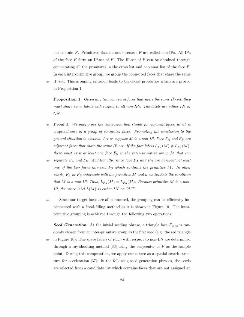
IP-set. This grouping criterion leads to beneficial properties which are proved480

in Proposition 1

Proposition 1. Given any two connected faces that share the same IP-set, they

must share same labels with respect to all non-IPs. The labels are either IN or

ON .

Proof 1. We only prove the conclusion that stands for adjacent faces, which is485

a special case of a group of connected faces. Promoting the conclusion to the

general situation is obvious. Let us suppose M is a non-IP. Face FA and FB are

adjacent faces that share the same IP-set. If the face labels LFA(M) 6= LFB

(M),

there must exist at least one face FS in the inter-primitive group M that can

separate FA and FB. Additionally, since face FA and FB are adjacent, at least490

one of the two faces intersect FS which contains the primitive M . In other

words, FA or FB intersects with the primitive M and it contradicts the condition

that M is a non-IP. Thus, LFA(M) = LFB

(M). Because primitive M is a non-

IP, the space label L(M) is either IN or OUT .

Since our target faces are all connected, the grouping can be efficiently im-495

plemented with a flood-filling method as it is shown in Figure 10. The intra-

primitive grouping is achieved through the following two operations:

Seed Generation. At the initial seeding phrase, a triangle face Fseed is ran-

domly chosen from an inter-primitive group as the first seed (e.g. the red triangle

in Figure 10). The space labels of Fseed with respect to non-IPs are determined500

through a ray-shooting method [36] using the barycenter of F as the sample

point. During this computation, we apply our octree as a spatial search struc-

ture for acceleration [37]. In the following seed generation phrases, the seeds

are selected from a candidate list which contains faces that are not assigned an

24

intra-primitive group. The candidate list is constructed in the process of label505

propagation.

Label propagation:. Before propagating labels, a new intra-primitive group is

created. But at the beginning, the group only contain the seed face Fseed only.

Start from the seed face Fseed, we use a breadth-first flood filling strategy to

visit all the faces that are connected to Fseed. For each visit, we check whether510

a visiting face has the same IP-set as the seed face Fseed. If the visiting face

shares the same IP-set as the seed, then it is inserted into the intra-primitive

group. Otherwise, it is pushed into a candidate list.

The intra-primitive grouping is accomplished through iterative repeating515

the above two operations for each primitive. The iteration stops until all the

faces are grouped. After the grouping, the inter-primitive groups generated in

the previous level are now divided into a series of intra-primitive groups. In

addition, according to Proposition 2, the space labels of the faces, which share

the same IP-set, share same space labels with respect to all non-IPs. We denote520

the set of space label determined with this feature as CLintra. Thus, the first

trimmed CSG tree generated in the previous level can be further trimmed using

CLintra. We named the CSG generated at the intra-primitive level as the

second trimmed CSG tree.

The bottleneck of the intra-primitive grouping lies in the space label eval-525

uation of the seeds. Evaluation through the ray-shooting method is time-

consuming and not suitable for complex CSG evaluation. Thus, we apply the

ray-shooting method to space labels of the initial seed only. For the space label

evaluation of the following seeds, we provide a more efficient solution taking

advantages of the information of neighboring faces.530

When adding a face Fcan into a candidate list in the label propagation phrase,

we associated the following data with Fcan: the current visiting face Fasso and

its space label with respects to its non-IPs. From the Figure 11, we can easily

know that Fcan and Fasso are adjacent to each other and have a common edge.

25

Figure 10: (left) A snapshot during flood filling; and (right) the final grouping result. Dif-

ferent intra-primitive groups are distinguished by different colors. From the final grouping

result, the whole mesh is divided into nine intra-primitive groups.

Let us denote the non-IP sets of Fcan and Fasso as Ican and Iasso respectively.535

When Fcan is selected as the new seed from the candidate list, its space label

evaluation can be evaluated by dividing the non-IP set Ican. For primitives

M ∈ Ican ∩ Iass, the value of LFcan(M) can be directly inherited from the

LFasso(M). For primitives M ∈ Ican − Iasso, the value of LFcan(M) can be

obtained by calculating the space label of any point on the common edge. To540

ensure robustness, the endpoints of the common edge is selected for calculation

in our implementation since we have their exact plane based representation.

The selection of sample point is guaranteed by the proposition 2.

Proposition 2. Given a primitive M and two adjacent faces, F1 and F2, if M

is in the IP-set of F2 but not in the IP-set of F1, the space label with respect to545

primitive M for F1 is the same as the label of any point on their common edge.

Proof 2. Since M is not in the IP-set of F1, all points on F1 have the same

space label with respect to M . For points on the common edge, they are attributed

26

Figure 11: Space label evaluation for seeds. Fcan is one of the secondary seeds in the

candidate list, and Fasso is its associated face. We can evaluate the space label of Fcan with

respect to different primitives according to the known space label from Fasso. The yellow,

blue and red lines within the triangles represented the intersection between the faces and the

primitive. For the yellow intersection, the primitive intersects Fasso only. Thus, the space

label of the Fcan with respect to this primitive can be obtained through a BSP-based point-

in-polygon test using any point on the common edge. For the blue intersection, the primitive

intersects both Fcan and Fasso, thus the space label is the same for both faces and allows

direct inherit from Fasso. For the red intersection, the primitive intersects Fcan only. Again,

we use the point-in-polygon test to obtain the space label with respect to this primitive.

to F1 and F2 simultaneously. Thus, for any point u on the common edge, we

have LF1(M) = Lu(M), where Lu(M) is the space label of the point u with550

respect to M .

6.2. Classification of the faces

The goal of face classification is to determine whether a face can be accepted

as a part of the final model or not. The classification can be conducted by

traversing the second trimmed CSG tree to obtain the final Boolean value. For555

non-intersected faces, the classification is simple and efficient for the CSG is

trimmed through our two-level grouping schemes and much of the unnecessary

evaluations are omitted.

For faces that intersect with other faces, further processing is needed to en-

sure robustness. Intersected faces usually cannot be classified as a whole. They560

have to be tessellated into smaller non-intersected triangles which need to be

classified separately. Extra classification suggests an increase in computation.

To pursue robustness and efficiency simultaneously, we embed the exact BSP

27

structure into the intersected faces for tessellation and sub-triangles classifica-

tion.565

6.2.1. Tessellation of intersected faces

Before dividing the intersected faces into a series of smaller triangles, we

classify the IPs of the intersected faces. If the IP of an intersected face is on the

second trimmed CSG tree, it is called a valid intersection primitive (valid-IP).

Otherwise, it is named as pseudo-intersection primitive (pseudo-IP). Pseudo-IPs570

intersect the face, but the space labels with respect to pseudo-IPs do not affect

the final classification of faces. In other words, the intersections of pseudo-IPs

are not edges of the final models, as shown in Figure 12. Thus, we simply omit

these pseudo-intersections during classification. This filtering saves computation

time by avoiding unnecessary splitting of faces. An extreme situation is that575

there is no valid-IP. In this situation, the face is processed the same way as a

non-intersected face.

Given an intersected face F , we divide it into a set of sub triangles using

the intersection information recorded in the detection phrase (See Section 5.2).

We convert the tessellation task into a problem of Constrained Delaunay Trian-580

gulation (CDT) [38], which has beneficial topological characteristics. The zone

of CDT is the face F , and the constraints are all the intersections marked by

valid-IPs. The constraints guarantee that no sub-triangles cross intersection

lines. To conduct CDT in 2D space, 3D coordinates in plane-based represen-

tation are projected as points on a 2D space, which is the axis-aligned plane585

where the area of F is maximized.

One critical issue that should be noted is that when the face F intersects

with different valid-IPs creating different intersections, these intersections may

also intersect each other as shown in Figure 13c. The intersections are reflected

as cross points on F . Omitting these points generated by the intersection of590

valid-IPs may cause incorrect results of CDT. To obtain the correct constraints,

these cross points are tested to determine whether an intersection exists or

not. We conduct the intersection test based on plane-based geometry to ensure

28

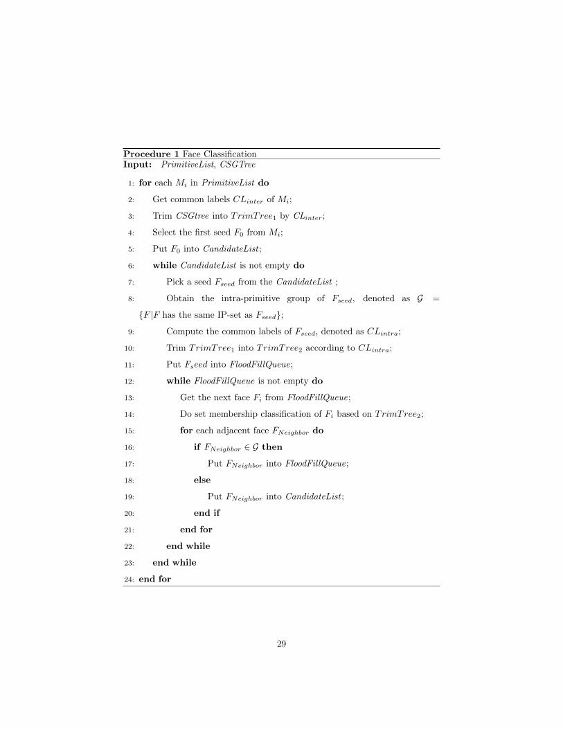
Procedure 1 Face ClassificationInput: PrimitiveList, CSGTree

1: for each Mi in PrimitiveList do

2: Get common labels CLinter of Mi;

3: Trim CSGtree into TrimTree1 by CLinter;

4: Select the first seed F0 from Mi;

5: Put F0 into CandidateList ;

6: while CandidateList is not empty do

7: Pick a seed Fseed from the CandidateList ;

8: Obtain the intra-primitive group of Fseed, denoted as G =

{F |F has the same IP-set as Fseed};

9: Compute the common labels of Fseed, denoted as CLintra;

10: Trim TrimTree1 into TrimTree2 according to CLintra;

11: Put Fseed into FloodFillQueue;

12: while FloodFillQueue is not empty do

13: Get the next face Fi from FloodFillQueue;

14: Do set membership classification of Fi based on TrimTree2;

15: for each adjacent face FNeighbor do

16: if FNeighbor ∈ G then

17: Put FNeighbor into FloodFillQueue;

18: else

19: Put FNeighbor into CandidateList ;

20: end if

21: end for

22: end while

23: end while

24: end for

29

Figure 12: 2D illustration of pseudo-intersection. The vertexes in red do not appear in the

final results. We called them pseudo-intersection vertexes.

robustness. According to our observation, the cross points are generated by the

intersection of three faces: the target intersected face F and two other faces595

from the valid-IPs that also intersected with F as shown in Figure 13d. Thus,

a cross point is able to be expressed with these three faces using plane-based

representation. Inspired by this idea, we can identify cross point through testing

whether a point is on all of these faces. Once the cross points are detected, the

constraints of CDT will be updated accordingly. Moreover, because the cross600

points are shared by the three faces we mentioned above, they are added to the

point lists of all these faces

6.2.2. Classification of sub-triangles

Through tessellation, the intersected face F is divided into a series of sub-

triangles. To enable efficient classification on these sub-triangles, we employ605

the Binary Space Partitioning (BSP) tree [26] to describe these triangles. A

BSP tree can express a divided entity using a tree structure. Partitions are

represented as leaves nodes in the tree and trunks represent binary partitioners.

The child nodes in the tree are formed by a binary partitioning of parents.

Although our tessellation is conducted on 2D space, we construct the BSP tree610

in 3D space. We assume the intersected face F has tiny thickness and denote

this imaginary thin plate. Let M be a valid-IP of F , we can easily partition the

plate into a 3D BSP-tree through inquiring the cross list and coplanar list of F .

The plate PF is divided into a series of cells. Each cell represents a sub-triangle

and is restored in the leave nodes of the BSP tree. There are advantages of615

30

Figure 13: Crossing between intersecting lines. When a face intersects with different primi-

tives, the generated intersecting lines may intersect each other and generate new points. (a)

face F intersects primitive M1; (b) face F intersects primitive M2; (c) the intersecting line

generated by F and M1 intersects the intersecting line generated by F and M2. The crossing

is marked with asteroid in red; (d) the crossing points of intersecting lines are in fact the

intersection of faces from different primitives.

utilizing a 3D BSP-tree instead of a 2D tree. On one hand, constructing 2D

BSP tree requires conversion of plane triples into coordinates. The conversion

inevitably introduced computational errors. On the other, building 3D BSP tree

allows us to use an exact plane-based method [6]. The intersection information

restored in advance (see section 5.2) using plane-based representation can be620

utilized directly.

After finishing construction of the BSP tree, the labels of a sub-triangle are

computed according to the space label of its vertexes. Given a sub-triangle FSub,

its label is determined by the results of the point-in-polygon test on its three

vertexes. If all the tree vertexes are labeled with ON , then space label of FSub625

with respect to a valid-IP M is either SAME of OPPO. If any vertex is not

labeled with ON , we can conclude that LFSub6= ON . When the space labels

of a sub-triangle respect to all primitives are computed, we determine whether

the sub-triangle belongs to the final model based on the second trimmed tree.

The sub-triangle is accepted if and only if the final evaluation result equals to630

SAME.

31

In the cases that the coplanar list of the intersected face F is empty or

the faces in the coplanar list are all from pseudo-IPs, acceleration is possible

for evaluating the final Boolean value of the sub triangles. In this situation,

the space labels of the sub-triangles with respect to valid-IPs are either IN or635

OUT and the CSG tree is, in fact, a binary tree. The evaluation of the second

trimmed CSG tree can be efficiently conducted using the Blister [39]. For CSG

models in which the coplanar cases are rare, this acceleration saves considerable

computation time.

7. Experimental Results640

We implemented our approach using C++ and tested a series of examples

with numerous primitives and faces on an Intel i5-4200D 1.5GHz processor with

8GB RAM. In our implementation, we employ the OpenMesh [40] for storing

triangle meshes and supporting the query performed by Constrained Delaunay

Triangulation using the Fade2D [41]. To verify the performance of our approach,645

we compare our approach with previous state-of-the-art techniques including

method by Campen et al. [2], the method by Feito et al. [5], the algorithm in

CGAL [22], the commercial solution in Autodesk Maya [42]. We also include

two non-incremental methods for comparison, QuickCSG [10] and method by

Zhou et al. [11] distributed in LibiGL. We analyze the performance of our ap-650

proach and other methods from four aspects: efficiency, time complexity, space

complexity and topology simplicity.

7.1. Efficiency

We conduct the Boolean evaluation with our approach and other methods

on numerous objects. Figure 14 shows some challenging examples whose geo-655

metric characteristics are shown in Table 1. The total number of faces in these

examples are large. Even a single primitive contains thousands of faces. Table

1 also presents the rumtime performance of our approach and other methods

on these examples. As it is shown in Table 1, our approach has advantages in

32

efficiency when compared to previous state-of-the-art techniques. Within the660

five incremental techniques for comparison, methods by Feito et al. [5] performs

the best but still have room for improvement when compared to our approach.

The runtime performance of the method by Feito et al. [5] in single Boolean

evaluation has a relatively small disadvantage compared to our approach. It

is because they also design a face-based grouping scheme for accelerating face665

membership classification. Thus both our approach and method by Feito et

al. [5] have similar pipelines for single Boolean operations. In the situation that

processing multi primitives, the efficiency of our non-incremental CSG evalua-

tion approach have obvious advantages over all four previous techniques. Figure

14(a) shows a difficult example which consists of 801 primitives. Methods by670

Feito et al. [5] fails to provide a proper evaluation. It takes more than 2000

seconds to finish the Boolean evaluation when applying method by Campen et

al. [2] and algorithm in CGAL [22]. Even with the mature solution in Autodesk

Maya [42], the time consumption is 1400 seconds. However, our approach only

uses 12.8 seconds to produce the correct results and is approximately 100 times675

faster than evaluating using Autodesk Maya [42]. When compares to the Li-

biGL [11], our approach still has advantages in efficiency. But when compared to

the QuickCSG, it is up to 2 times faster than our approach. The relatively small

performance difference between our approach and an inexact method indicates

that our approach presents a reasonable performance.680

7.2. Time Complexity

We analyze the time complexity of each phase in our approach. As we have

described in Section 4, our approach contains three phases: octree-construction,

intersection computation, and face classification. The octree-construction we

applied is a typical O(n log n) method, where n is the number of faces in CSG. In685

phase 2, intersection computation is conducted within the critical cells in octree

only. The number of critical cells is often linear to the number of intersected

faces k in CSG (k often approximately equals to√n). Thus, the time complexity

of intersection computation is O(k).

33

Figure 14: (a) Boolean operations between a Ring and a set of Spheres, 〈1〉 after 200 opera-

tions, 〈2〉 after 800 operations; (b) Armadillo ∪ six Spoons; (c) Head - Cuboid + LeftBrain +

RightBrain; (d) Difference between a BigCylinder and 28 SmallCylinders; (e) Man ∪ Horse;

(f) Dragon - Bunny; and (g) Palate ∪ Mandible ∪ (20 Teeth).

34

Figure 15: Boolean operations on model Buddha. (a) two Buddhas; (b) our result of Buddha

∩ Buddha; (c) incorrect result of Buddha ∩ Buddha generated by method [5]; (e) lion; (f)

Buddha ∪ Lion by our approach; (g) Results by QuickCSG [10]. There are numerous cavities

on the model.

Table 1: Computation Time Statistics of the Evaluations of Large CSGs (Seconds)

Example FigureFace Num.∇ Num. of

Primitives

CGAL

[22]

Maya

[42]

Campen

et al. [2]

Feito

et al. [5]

QuickCSG

[10]

LibiGL

[11]

Our Approach

Total Min Max Total◦ Phase 1 Phase 2 Phase 3

Ring ∩ Spheres (200 times) 14(a)-1 37.6K 180 1.6K 201 1350 49.9 TLE † 15.9 1.7 57.9 3.13 0.328 1.69 0.922

Ring ∩ Spheres (800 times) 14(a)-2 146K 180 1.6k 801 TLE 1400 TLE Fail∗ 6.42 236.8 12.8 1.36 6.41 4.00

Armadillo ∪ 6 Spoons 14(b) 377k 2.56K 346K 7 TLE 224.5 45.7 11.7 0.69 26.64 1.44 0.438 0.062 0.563

Head− Cuboid+ LeftBrain+RightBrain 14(c) 79.2K 12 38.2K 4 97.6 Fail 3.58 1.69 0.33 10.41 0.563 0.187 0.141 0.172

BigCylinder − 28 SmallCylinder 14(d) 36K 800 2.4K 29 34.1 7.03 18.7 4.05 0.16 5.79 0.313 0.094 0.094 0.081

Man ∪Horse 14(e) 597k 96.9K 500K 2 TLE 38.3 26.4 5.63 1.06 39.4 2.13 0.563 0.031 0.984

Dragon−Bunny 14(f) 170K 69.7K 100K 2 218 7.45 13.8 2.39 0.45 16.48 0.891 0.328 0.125 0.266

Palate ∪Mandible ∪ 20Teeth 14(g) 362K 6.91K 276K 22 TLE 344 256 19.2 0.8 33.3 1.80 0.766 0.172 0.593

Buddha ∩Buddha 15 2.16M 1.08M 1.08M 2 Fail Fail MLE ] Fail 5.66 209.05 11.3 5.55 1.36 3.01

Buddha ∪ Lion 15 2.55M 1.06M 1.08M 2 Fail Fail MLE Fail 7.07 235.5 13.65 5.65 1.56 6.44

∇ Min (Max) means the minimum (maximum) number of faces of a single primitive;

◦ The total computation time of our method includes the construction of half-edge structure and

the three steps in Section 4;

∗ Fail means nothing was returned, or we received the wrong evaluation results from the programs;

† TLE means the processing time was more than 2, 000 seconds;

] MLE denotes that the program was out of memory.

35

The time complexity of the final phase varies according to the conditions of690

the objects. For the grouping schemes in this phase, the flood-filling method we

applied has a complexity of O(n). For the classification operation in this face,

the time consumption for classification intersected faces and non-intersected

faces varies. Classifying intersected faces may take much more time than clas-

sifying non-intersected faces. The time for classifying non-intersected faces is695

negligible. Thus, base on the assumption that classifying a non-intersected face

incurs no computational time, the time complexity of the third phase is approx-

imately O(n + θk), where θ is a parameter between 1 and 0. Specially, when

k/n is constant, the time complexity of the third phase reduces to O(n).

We monitor the time changes when the number of primitives grows to provide700

further evidence of our time complexity analysis. Table 2, shows the evaluation

time for Figure 14(a), which is a CSG consisting of a ring and hundreds of

identical spheres. We change the number of spheres from 100 to 800 and record

the evaluation times. In these experiments, the k/n can be relatively regarded

as a constant. Thus, phase 2 and 3 occupy a majority of the computing time.705

As it is shown in Table 2, the computational time of our approach has an O(n)

performance, which is accord to our analysis. The computation time of other

incremental methods rapidly inflates when the number of primitives increases,

sometimes showing O(n2) behavior. When spheres are added to or subtracted

from the ring, the mesh of the ring becomes more and more complex with710

the incremental methods. Thus, subsequent Boolean operations are difficult

to perform in the later periods of these methods. When compared to the non-

incremental LibiGL [11], our approach still has advantages in computation time.

When compared to fastest the method QuickCSG, our approach has a relatively

small disadvantage and is still competitive.715

7.3. Space Complexity

One possible problem of conducting a non-incremental CSG evaluation is

memory consumption. Unlike incremental methods, non-incremental approaches

often require loading all the primitives into the memory before the evaluation.

36

Table 2: Number of Primitives and Computation Time (Seconds)

Number of SpheresComputation time

CGAL [22] Maya [42] Feito et al. [5] QuickCSG [10] LibiGL [11] Our approach

100 439 17.4 5.20 0.69 25.53 1.38

200 1350 53.4 15.9 1.44 53.47 2.89

300 - 124 30.4 2.2 81.21 4.39

400 - 241 - 2.98 110.4 5.97

500 - 407 - 3.95 146.1 7.90

600 - 628 - 4.74 175.6 9.49

700 - 966 - 5.5 203.5 11.0

800 - 1400 - 6.24 236.8 12.8

Fortunately, our approach does not significantly suffer from memory limitation.720

In our approach, the memory loading operation mainly conducted in the phase

of octree construction. In this phase, the size of our constructed octree is typi-

cally an O(n log n). The auxiliary information of intersected faces, which usually

has a size of O(k), is also loaded into the memory in this phase. Experimen-

tal results show that our approach is able to perform full evaluation in Table725

1 with less than 600MB memory. On contrary, some incremental approaches

suffer from the mass memory occupation. For instance, in the evaluation of

Figure 14e, CGAL [22] consumed more than 6GB memory. Furthermore, in

the evaluation of Example 2 in Figure 14a, which contained only 146K faces,

at least 5GB memory is used by Maya [42].730

7.4. Topological Simplicity

Topological simplicity refers to the number of triangles used in the final

models. It is also an important aspect for evaluating the quality of CSG. A

simpler topology is preferred for it provides convenient for further process. As

shown in Figure 16, our method used fewer triangles to represent final model735

than [2] without extra surface merging. Table 3 shows the triangles used in the

final mesh model by our approach and other methods. We suggest that the

topology simplicity is related to the efficiency of the methods. Improper tessel-

lation method may cause inefficiency when the model is smashed into numerous

pieces. Through a closer study on the evaluation process of Figure 14a, we740

37

Table 3: Comparison of Topology SimplicityMethods CGAL [22] Maya [42] Campen et al. [2] Feito et al. [5] QuickCSG [10] LibiGL [11] Our approach

Number of Triangles (Under 1283 resolution)

Cube ∪ Sphere 1 ∩ Sphere 2 (Figure 16)19.21K 12.85K 19.9K 15K 4.77K 6.93K 3.9K

notice that after hundreds of Boolean operations, the surface of the models are

fragemented into massive sub faces in the method by Campen et al. [2]. Thus,

it takes more than ten seconds to perform a Boolean operation. Through the

above observation, we notice that the topology simplicity is closely related to

the tessellation of faces.745

The tessellation of the faces also influences the robustness of the evaluation.

Our two-level grouping schemes provide a sound foundation for the tessella-

tion and avoid unnecessary operations. In our experiments, our approach can

correctly evaluate all the models in Table 1. However, our compared methods

suffered from different kinds of problems. Maya [42] failed to evaluate Figure750

14c, which contained only 79.2K faces and four primitives. CGAL [22] showed

warnings when evaluating Figure 15a and finally terminated without returning

a result. The method by Feito et al. [5] returned an incorrect result for the eval-

uation of Figure 15a. The returned result is shown in Figure 15c which contains

incorrect cavities. Although our approach have a slight disadvantage in effi-755

ciency when compared with QuickCSG [10], it is worth to notice that QuickCSG

is easy to generate deficit result when the genral position assumption is violated.

Although our approach performs robustly in our experiments, we have to admit

that our face tessellation is not unconditionally robust. Because the tessellation

of intersected faces is performed using vertex-based representation, the coor-760

dinates of the vertexes may shift from their real location, which may lead to

incorrect tessellation. A potential solution is to integrate plane-based geometry

computation into the intersected face tessellation process.

8. Conclusion

In this paper, we proposed an efficient non-incremental approach to evaluate765

the constructive solid geometry (CSG) with triangular mesh primitives. Our

38

Figure 16: Cube ∪ Sphere 1 ∩ Sphere 2. The result of our approach has a simpler topology

than that of other methods.

approach performs very efficiently for non-incremental evaluation of large CSG

with massive faces. The key contribution of our approach is to apply the local

coherence of face space labels to accelerate the face membership classification

process. A two-level grouping framework is developed to group the neighboring770

faces together. Space labels are then propagated within each group. Our scheme

saves considerable time for space label evaluation, which is an important time-

consuming operation for the conventional Boolean evaluations. In addition, to

strengthen robustness, plane-based geometry computation is introduced into

the intersection computing process of our approach. Multiple experiments have775

shown that our approach has high efficiency while retaining high robustness and

stability.

Acknowledgments

The work is supported by the National Natural Science Foundation of China

(No. 61572316, 61632003, 61672502), Macao Foundation, National High-tech780

R&D Program of China (863 Program) (No. 2015AA015904), the Key Program

for International S&T Cooperation Project of China (No. 2016YFE0129500),

the Science and Technology Commission of Shanghai Municipality (No. 16DZ0501100,

17411952600), the Interdisciplinary Program of Shanghai Jiao Tong University

39

(No. 14JCY10), the Research Grants Council of the Hong Kong Special Admin-785

istrative Region, China (No. CityU 11237116), City University of Hong Kong

(No. 7004915), and ACIM-SCM.

References

[1] Requicha, Aristides, A.G, Mathematical models of rigid solid objects, Uni-

versity of Rochester.790

[2] C. Marcel, K. Leif, Exact and robust (self-)intersections for polygonal

meshes, Computer Graphics Forum 29 (2) (2010) 397–406.

[3] D. Pavi, M. Campen, L. Kobbelt, Hybrid Booleans, Computer Graphics

Forum 29 (1) (2010) 75–87.

[4] C. C. L. Wang, Approximate Boolean operations on large polyhedral solids795

with partial mesh reconstruction, IEEE Transactions on Visualization and

Computer Graphics 17 (6) (2010) 836–849.

[5] F. R. Feito, C. J. Ogayar, R. J. Segura, M. L. Rivero, Fast and accurate

evaluation of regularized Boolean operations on triangulated solids, Cad

Computer Aided Design 45 (3) (2013) 705–716.800

[6] G. Bernstein, D. Fussell, Fast, exact, linear Booleans, Computer Graphics

Forum 28 (5) (2009) 1269–1278.

[7] J. Hable, J. Rossignac, CST: Constructive solid trimming for render-

ing BReps and CSG, IEEE Transactions on Visualization and Computer

Graphics 13 (5) (2007) 1004.805

[8] J. Rossignac, Ordered Boolean list (OBL): Reducing the footprint for eval-

uating Boolean expressions, IEEE Transactions on Visualization and Com-

puter Graphics 17 (9) (2011) 1337–1351.

40

[9] M. Granados, P. Hachenberger, S. Hert, L. Kettner, K. Mehlhorn, M. Seel,

Boolean operations on 3D selective nef complexes: Data structure, al-810

gorithms, and implementation, in: European Symposium on Algorithms,

2003, pp. 654–666.

[10] M. Douze, J.-S. Franco, B. Raffin, QuickCSG: Arbitrary and faster Boolean

combinations of n solids, Ph.D. thesis, Inria-Research Centre Grenoble–

Rhone-Alpes; INRIA (2015).815

[11] Q. Zhou, E. Grinspun, D. Zorin, A. Jacobson, Mesh arrangements for solid

geometry, ACM Transactions on Graphics (TOG) 35 (4) (2016) 39.

[12] C. K. Yap, Robust geometric computation, in: Handbook of discrete and

computational geometry, CRC Press, Inc., 1997, pp. 653–668.

[13] A. A. G. Requicha, H. B. Voelcker, Boolean operations in solid modeling:820

Boundary evaluation and merging algorithms, Proceedings of the IEEE

73 (1) (1985) 30–44.

[14] D. H. Laidlaw, W. B. Trumbore, J. F. Hughes, Constructive solid geometry

for polyhedral objects, international conference on computer graphics and

interactive techniques 20 (4) (1986) 161–170.825

[15] R. P. K. Banerjee, J. Rossignac, Topologically exact evaluation of polyhedra

defined in CSG with loose primitives, Computer Graphics Forum 15 (4)

(1996) 205–217.

[16] S. Fortune, Polyhedral modelling with exact arithmetic, acm symposium

on solid modeling and applications (1995) 225–234.830

[17] J. Keyser, T. Culver, M. Foskey, S. Krishnan, D. Manocha, Esolid–a system

for exact boundary evaluation, Computer-aided Design 36 (2) (2004) 175–

193.

[18] P. Hachenberger, L. Kettner, Boolean operations on 3D selective nef com-

plexes: optimized implementation and experiments, solid and physical835

modeling (2005) 163–174.

41

[19] S. Fang, B. D. Bruderlin, X. Zhu, Robustness in solid modelling: a

tolerance-based intuitionistic approach, Computer-aided Design 25 (9)

(1993) 567–576.

[20] C. Hu, N. M. Patrikalakis, X. Ye, Robust interval solid modelling part i:840

representations, Computer-aided Design 28 (10) (1996) 807–817.

[21] M. Segal, Using tolerances to guarantee valid polyhedral modeling results,

international conference on computer graphics and interactive techniques

24 (4) (1990) 105–114.

[22] P. Hachenberger, L. Kettner, 3D Boolean operations on Nef polyhedra, in:845

CGAL User and Reference Manual, 3.9 Edition, CGAL Editorial Board,

2011.

[23] K. Sugihara, M. Iri, A solid modelling system free from topological incon-

sistency, Journal of Information Processing 12 (4) (1990) 380–393.

[24] J. R. Shewchuk, Lecture notes on geometric robustness, in: Interpola-850

tion, Conditioning, & Quality Measures in Eleventh International Meshing

Roundtable, 1999, pp. 115–126.

[25] W. C. Thibault, B. F. Naylor, Set operations on polyhedra using binary

space partitioning trees, international conference on computer graphics and

interactive techniques 21 (4) (1987) 153–162.855

[26] B. Naylor, J. Amanatides, W. C. Thibault, Merging bsp trees yields poly-

hedral set operations, Computers & Graphics.

[27] J. R. Shewchuk, Adaptive precision floating-point arithmetic and fast ro-

bust geometric predicates, Discrete and Computational Geometry 18 (3)

(1997) 305–363.860

[28] C. C. Wang, D. Manocha, Efficient boundary extraction of bsp solids based

on clipping operations, IEEE transactions on visualization and computer

graphics 19 (1) (2013) 16–29.

42

[29] H. Zhao, C. C. L. Wang, Y. Chen, X. Jin, Parallel and efficient Boolean on

polygonal solids, The Visual Computer 27 (2011) 507–517.865

[30] K. Museth, D. E. Breen, R. T. Whitaker, A. H. Barr, Level set surface

editing operators, international conference on computer graphics and in-

teractive techniques 21 (3) (2002) 330–338.

[31] H. Chen, S. Fang, A volumetic approach to interactive CSG modeling and

rendering, ACM Symposium on Solid Modeling and Applications (1999)870

318–319.

[32] E. Eisemann, X. Decoret, Single-pass GPU solid voxelization for real-time

applications, in: Graphics Interface, 2008, pp. 73–80.

[33] S. Gottschalk, M. C. Lin, D. Manocha, Obbtree: a hierarchical structure for

rapid interference detection, international conference on computer graphics875

and interactive techniques (1996) 171–180.

[34] T. Moller, A fast triangle-triangle intersection test, Journal of Graphics

Tools 2 (2) (1997) 25–30.

[35] J. R. Rossignac, H. B. Voelcker, Active zones in CSG for accelerating

boundary evaluation, redundancy elimination, interference detection, and880

shading algorithms, ACM Transactions on Graphics (TOG) 8 (1) (1988)

51–87.

[36] V. Havran, A summary of octree ray traversal algorithms, Ray Tracing

News 12 (2) (1999) 11–23.

[37] S. F. Frisken, R. N. Perry, Simple and efficient traversal methods for885

quadtrees and octrees, Journal of Graphics Tools 7 (3) (2002) 1–11.

[38] L. P. Chew, Constrained delaunay triangulations, Algorithmica 4 (1-4)

(1989) 97–108.

43

[39] J. Hable, J. Rossignac, Blister: GPU-based rendering of Boolean combi-

nations of free-form triangulated shapes, ACM Transactions on Graphics890

24 (3) (2005) 1024–1031.

[40] M. Botsch, S. Steinberg, S. Bischoff, L. Kobbelt, OpenMesh: A generic and

efficient polygon mesh data structure, in: OpenSG Symposium, 2002, pp.

1–5.

[41] Geom, Fade2D, http://www.geom.at/fade2d/html (2017).895

[42] Autodesk, Autodesk Maya, https://www.autodesk.com.hk/products/

maya/overview (2017).

44