Numerical study of the incremental unknowns method
25
Numerical Study of the Incremental Unknowns Method Salvador Garcia Laboratoire d'Analyse Numerique, Universite Paris XI, Bstiment 425, 91405 Orsay, France Received 2 July 1992; revised manuscript received 14 January 1993 Through numerical experiments we explore the incremental unknowns method; linear stationary as well as evolutionary problems are considered. For linear stationary problems, the method appears as a nearly optimal two-step preconditioning technique. At each step, we observe that the convergence behavior of the iterative methods employed is dramatically different, depending upon whether or not preconditioning is used. For linear evolutionary problems, successful and sharply accurate long-term integration is observed when the incremental unknowns (other than that of the coarsest level) are, effectively, small quantities. Otherwise. systematical aliasing arises. 0 1994 John Wiley & Sons, Inc. 1. INTRODUCTION Our objective in this article is to bring forward the numerical (computational) framework suitable to examine two-dimensional second-order Dirichlet boundary-value problems, and their associated initial boundary-value problems, by means of the incremental unknowns method [ 11 when several levels of discretization are considered. The method is set up in two steps. First, the two-dimensional second-order Dirichlet boundary-value problem is discretized with central differences on the finest grid. Next, quadratic interpolation is used to recursively define the incremental unknowns (other than that of the coarsest level). Since the discretization of the problem is fixed (on the finest level), the method, as a whole, is not recursive. Now, the hierarchical ordering of the primitive (nodal) unknowns introduced in [2] lead to a linear system (A) (X) = (b), which can be written, with the use of the incremental unknowns ordered in the same way, as the equivalent system [A][X] = [b], where [A] = Sr(A)S and [b] = ST(b). Here, S stands for the transfer matrix from the incremental unknowns [XI to the primitive (nodal) unknowns (X), i.e., (X) = S[X]. The explicit block-matrix structure of the matrix S, of the matrix R = STS, and of the matrix [TI, where [TI = ST(T)S, for any (second- or first-order) finite-difference operator T, has been given in [2]. We deduce that the block diagonal part of [A] is extremely simple. Indeed, at the coarsest level we obtain a block tridiagonal matrix with tridiagonal blocks; at all other levels (defined by the hierarchical ordering of the unknowns) we obtain, successively, a tridiagonal or diagonal matrix. Numerical Methods for Partial Differential Equations, 10, 103- 127 (1994) 0 1994 John Wiley & Sons, Inc. CCC 0749-159X/94/010103-25
-
Upload
independent -
Category
Documents
-
view
4 -
download
0
Transcript of Numerical study of the incremental unknowns method
Numerical Study of the Incremental Unknowns Method Salvador Garcia Laboratoire d'Analyse Numerique, Universite Paris XI, Bstiment 425, 91405 Orsay, France
Received 2 July 1992; revised manuscript received 14 January 1993
Through numerical experiments we explore the incremental unknowns method; linear stationary as well as evolutionary problems are considered. For linear stationary problems, the method appears as a nearly optimal two-step preconditioning technique. At each step, we observe that the convergence behavior of the iterative methods employed is dramatically different, depending upon whether or not preconditioning is used. For linear evolutionary problems, successful and sharply accurate long-term integration is observed when the incremental unknowns (other than that of the coarsest level) are, effectively, small quantities. Otherwise. systematical aliasing arises. 0 1994 John Wiley & Sons, Inc.
1. INTRODUCTION
Our objective in this article is to bring forward the numerical (computational) framework suitable to examine two-dimensional second-order Dirichlet boundary-value problems, and their associated initial boundary-value problems, by means of the incremental unknowns method [ 11 when several levels of discretization are considered.
The method is set up in two steps. First, the two-dimensional second-order Dirichlet boundary-value problem is discretized with central differences on the finest grid. Next, quadratic interpolation is used to recursively define the incremental unknowns (other than that of the coarsest level). Since the discretization of the problem is fixed (on the finest level), the method, as a whole, is not recursive. Now, the hierarchical ordering of the primitive (nodal) unknowns introduced in [2] lead to a linear system (A) ( X ) = (b) , which can be written, with the use of the incremental unknowns ordered in the same way, as the equivalent system [ A ] [ X ] = [b ] , where [ A ] = Sr(A)S and [b] = ST(b) . Here, S stands for the transfer matrix from the incremental unknowns [XI to the primitive (nodal) unknowns ( X ) , i.e., ( X ) = S [ X ] . The explicit block-matrix structure of the matrix S, of the matrix R = S T S , and of the matrix [ T I , where [TI = S T ( T ) S , for any (second- or first-order) finite-difference operator T , has been given in [2]. We deduce that the block diagonal part of [ A ] is extremely simple. Indeed, at the coarsest level we obtain a block tridiagonal matrix with tridiagonal blocks; at all other levels (defined by the hierarchical ordering of the unknowns) we obtain, successively, a tridiagonal or diagonal matrix.
Numerical Methods for Partial Differential Equations, 10, 103- 127 (1994) 0 1994 John Wiley & Sons, Inc. CCC 0749-159X/94/010103-25
104 GARCIA
Hereafter, we always solve the linear system [A][X] = [b], instead of the linear system (A)(X) = (b) , with the use of the following iterative methods: the conjugate gradient method when [A] is a symmetric positive definite matrix, and the CGSTAB method introduced in [ 5 ] otherwise. These iterative schemes are, in fact, applied to the linear system X-'[A][X] = X-'[b], where X = blockdiag[A], that is, block diagonal scaling preconditioning is used. In our case, the implementation of such a methodology is straightforward.
We point out that, for a grid fuced, the best convergence behavior is, systematically, obtained in the rwo-level case. In addition, as the number of levels increases (the size of the coarsest grid diminishes), more and more iterations are required to attain the discretization accuracy.
For linear evolutionary problems, we have to solve, at each time step, an incremental unknowns linear system; this is accomplished following the precedent guidelines. For the heat equation successful and sharply accurate long-term integration is observed when the incremental unknowns (other than that of the coarsest level) are, effectively, small quantities. Otherwise, systematical aliasing arises.
Reference [ 2 ] and the exposition presented hereafter altogether provide deeper insight into the incremental unknowns method and produce new techniques to study the long-term integration of dissipative evolutionary equations.
This article is organized as follows. In Sec. I1 we briefly recall the matricial framework for the incremental unknowns method when several levels of discretization are considered. In Sec. 111 we discuss iterative methods and preconditioning techniques. In Sec. IV we present a fast algorithm for computing the products of the matrices S and S T with a vector. In Sec. V, through numerical experiments, we explore the incremental unknowns method. Linear stationary as well as evolutionary problems are considered. Finally, in Sec. V1, we state some concluding remarks.
It. INCREMENTAL UNKNOWNS METHOD
In this section we will briefly recall the matricial framework for the incremental unknowns (IU) method when several levels of discretization are considered; for a detailed report, see [ 2 ] . We will again describe the block diagonal part of the underlying matrices since the explicit knowledge of such blocks will be very helpful when using preconditioning techniques in conjunction with blockwise iterative methods.
Here, we consider the two-dimensional Dirichlet boundary-value problem
u = O o n I ' = a l n , (4 where S, p , 8, a , p, y are given constants.
Let i , N be non-negative integers, i , N 2 2, remaining fixed. We set h = 1/2'- 'N and, for j = 0,. . . , i - 1, we introduce the uniform grid a,, of level j , corresponding to the mesh size hj = 2'-j-'h in both directions; therefore we obtain the nested sequence of grids
ni-1 3 ai-2 3 ... 3 R1 3 RrJ. (3)
NUMERICAL STUDY OF THE INCREMENTAL UNKNOWNS METHOD 105
The problem (1) and (2) is discretized with central differences on the finest grid so that its finite-difference approximation is
(4) ( 8 ~ x . x + p ~ y y + e ~ x y + ~ A P + + yz)urn,n = f m , n
m , n = 1 ,..., 2’- ’N - 1,
where we designate by f r n , n = f ( m h , nh) the exact values o f f and by the approximate values of u at the nodes of the grid A: are the standard (centered) finite-difference operators approximating the derivatives
= u(mh, nh) Furthermore, Axx, Ayy, Axy, A:,
a* a* a2 a a ax2’ ay*’ ax a y ’ a x ’ a y ’
respectively. Now, the finite-difference approximation (4) and the hierarchical ordering of the
primitive (nodal) unknowns introduced in [2] lead to a linear system ( A ) ( X ) = (b ) , which can be written, with the use of the incremental unknowns (see [l-31) ordered in the same way, as the equivalent system [ A ] [XI = [ b ] , where [ A ] = S T ( A ) S and [b] = ST(b) . Here, S stands for the transfer matrix from the incremental unknowns [XI to the primitive (nodal) unknowns ( X ) , i.e., ( X ) = S [ X ] . The explicit block-matrix structure of the matrix S, of the matrix R = STS, and of the matrix [ T I , where [TI = S T ( T ) S , for any (second- or first-order) finite-difference operator T , has been given in [2]. Next, we proceed to recall the block diagonal part of such matrices.
To begin with, we now introduce some notation. Let k , u be non-negative integers, (T E G = (0, 1). We set
N ( k ; a ) = 2 k - 1 N - u , F = 1 - U . (5 ) Moreover, we introduce the quantities
2 x; , j = f ( 2 ‘ - j + %),
Finally, we will denote by A 63 B the tensor product of the matrices A and B, by AT the transpose of the matrix A , by I N the identity matrix of order N , and by [ x , y , z I N , x , y , z E 08, the tridiagonal matrix of order N X N :
Besides this, we will denote by a;,, the Kronecker delta.
A, = 6,,oAxx + 6C,1Ay:i7
For convenience, we will write
V, = 6,,oA: + S,,1A!.
I X N
106 GARCIA
where
[TI = ST(T)S, T = A,, Axyr V, and
l /h2 , if T = A,, c (T) = 1/4h2, if T = dry, t 1/2h, if T = Q,.
We can now state the following results (see [2]): The block diagonal part of [A,] is given by
(13)
j = 1 , ..., i - 1 , u E G .
The block diagonal part of [Axy] is given by
[Axyll , l = [-l,0711N-l @ [ - 1 A 1 l N - I 7 (23)
(24) [Axy]2j+o,2j+o = 0, j = 1 , . . . , i - 1, u E G .
We will also approximate the derivatives d/ax and d/dy by uncentered (backward or forward) first-order accurate finite differences; we will denote by A;, A; (backward), A:, A; (forward) the corresponding finite-difference operators. Now, the block-matrix structure of [V:], where V: = 6,,0A: + aC, ]A;, folIows readily from the relationships
1 y(v: + v,) = v,, V: - V; = hA, .
NUMERICAL STUDY OF THE INCREMENTAL UNKNOWNS METHOD 107
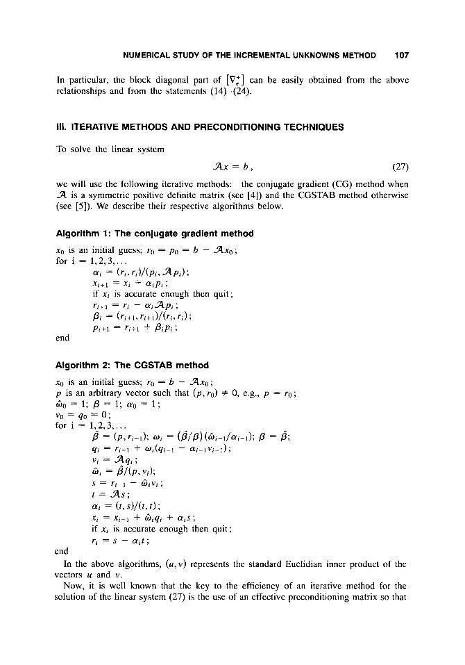
In particular, the block diagonal part of [V:] can be easily obtained from the above relationships and from the statements (14)-(24).
111. ITERATIVE METHODS AND PRECONDITIONING TECHNIQUES
To solve the linear system
A x = b , (27)
we will use the following iterative methods: the conjugate gradient (CG) method when A is a symmetric positive definite matrix (see [4]) and the CGSTAB method otherwise (see [5]) . We describe their respective algorithms below.
Algorithm 1: The conjugate gradient method
xo is an initial guess; ro = po = b - 3 x 0 ; for i = 1,2,3, . . .
ai = ( T i , r i ) l (p i* A p i ) ; X i + [ = xi + a i p i ; if xi is accurate enough then quit; r i + l = ri - a i A p i ; pi = ( r i+ l . r i+ i ) / ( r i , r l ) ; pi+l = ri+l + P i p i ;
end
Algorithm 2: The CGSTAB method
xo is an initial guess; ro = b - 3 x 0 ; p is an arbitrary vector such that ( p , ro) f 0, e.g., p = ro; Go = 1; p = 1; a0 = 1; vo = q o = 0 ; for i = 1,2,3, ...
P = (P, ri-1); oi = ( P / P ) ( G i - l / a i - l ) ; P = 8; qi = T i - l + W i ( q i - 1 - ai -Iv i -1) ; vi = Aq1 ; Gi = @ / ( p , v i ) ;
r = A s ; ai = (r, s > / ( f , r) ; x . 1 = x . 1 - 1 + G , q , + a i s ;
s = - G . v . . 1 1 9
if xi is accurate enough then quit; ri = s - air;
end In the above algorithms, (u,v) represents the standard Euclidian inner product of the
vectors u and v . Now, it is well known that the key to the efficiency of an iterative method for the
solution of the linear system (27) is the use of an effective preconditioning matrix so that
108 GARCIA
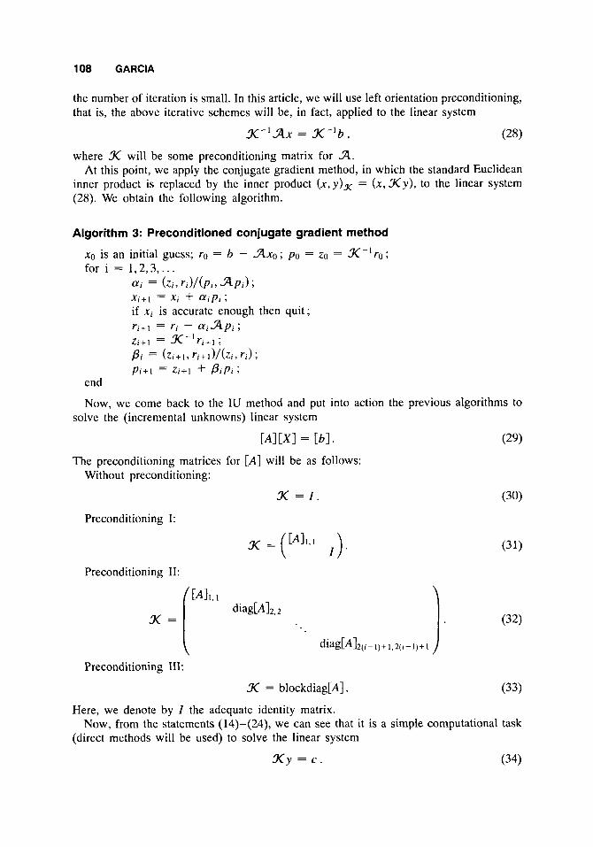
the number of iteration is small. In this article, we will use left orientation preconditioning, that is, the above iterative schemes will be, in fact, applied to the linear system
K F I A x = K-lb, (28) where X will be some preconditioning matrix for 3.
At this point, we apply the conjugate gradient method, in which the standard Euclidean inner product is replaced by the inner product ( x , ~ ) ~ = (x, X y ) , to the linear system (28). We obtain the following algorithm.
Algorithm 3: Preconditioned conjugate gradient method
xo is an for i =
end
Now, we come back to the IU method and put into action the previous algorithms to solve the (incremental unknowns) linear system
[A]" = [b l . (29)
The preconditioning matrices for [A] will be as follows: Without preconditioning:
X = I . (30)
Preconditioning I:
Preconditioning 11:
Preconditioning 111:
K = blockdiag[A]. (33)
Here, we denote by I the adequate identity matrix.
(direct methods will be used) to solve the linear system Now, from the statements (14)-(24), we can see that it is a simple computational task
X y = c . (34)
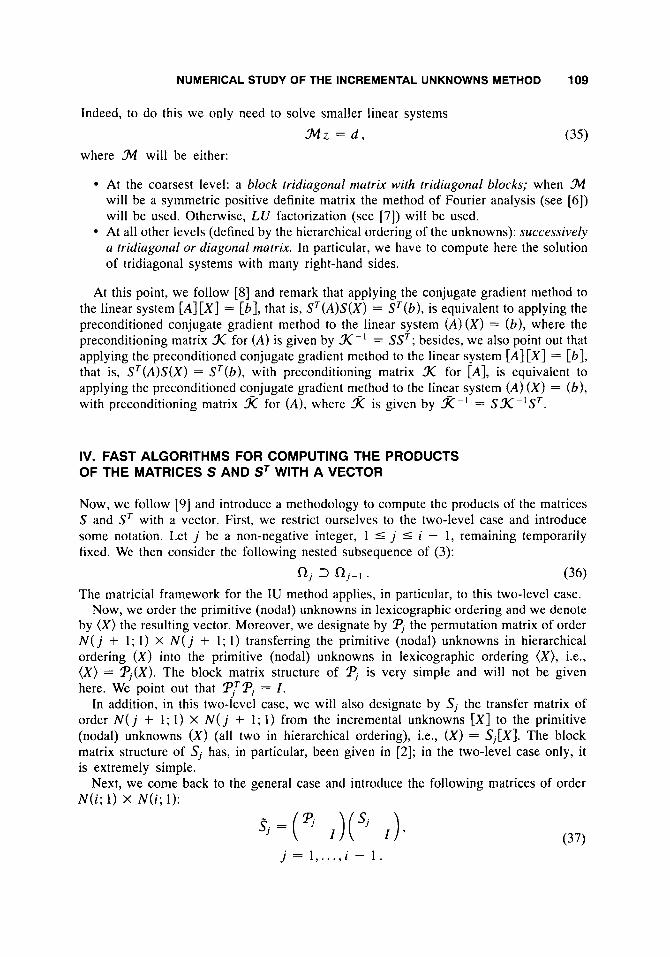
NUMERICAL STUDY OF THE INCREMENTAL UNKNOWNS METHOD 109
Indeed, to do this we only need to solve smaller linear systems
N z = d , (35) where N will be either:
At the coarsest level: a block tridiagonal matrix with tridiagonal blocks; when N will be a symmetric positive definite matrix the method of Fourier analysis (see [6]) will be used. Otherwise, LU factorization (see [7]) will be used. At all other levels (defined by the hierarchical ordering of the unknowns): successively a tridiagonal or diagonal matrix. In particular, we have to compute here the solution of tridiagonal systems with many right-hand sides.
At this point, we follow [8] and remark that applying the conjugate gradient method to the linear system [ A ] [XI = [b ] , that is, S T ( A ) S ( X ) = S r ( b ) , is equivalent to applying the preconditioned conjugate gradient method to the linear system ( A ) ( X ) = (b) , where the preconditioning matrix .K for ( A ) is given by K- ' = S S T ; besides, we also point out that applying the preconditioned conjugate gradient method to the linear system [ A ] [XI = [ b ] , that is, S T ( A ) S ( X ) = S T ( b ) , with preconditioning matrix .K for [ A ] , is equivalent to applying the preconditioned conjugate gradient method to the linear system ( A ) ( X ) = (b) , with preconditioning matrix x for ( A ) , where x is given by x-' = S 3 ( - ' S T .
IV. FAST ALGORITHMS FOR COMPUTING THE PRODUCTS OF THE MATRICES S AND ST WITH A VECTOR
Now, we follow [9] and introduce a methodology to compute the products of the matrices S and S T with a vector. First, we restrict ourselves to the two-level case and introduce some notation. Let j be a non-negative integer, 1 5 j 5 i - 1, remaining temporarily fixed. We then consider the following nested subsequence of (3):
a, 3 nip'. (36) The matricial framework for the IU method applies, in particular, to this two-level case.
Now, we order the primitive (nodal) unknowns in lexicographic ordering and we denote by ( X ) the resulting vector. Moreover, we designate by ;pJ the permutation matrix of order N ( j + 1; 1) X N ( j + 1; 1) transferring the primitive (nodal) unknowns in hierarchical ordering ( X ) into the primitive (nodal) unknowns in lexicographic ordering ( X ) , i.e., ( X ) = P j ( X ) . The block matrix structure of Pj is very simple and will not be given here. We point out that qT;pJ = I .
In addition, in this two-level case, we will also designate by sj the transfer matrix of order N ( j + 1; 1) X N ( j + 1; 1) from the incremental unknowns [XI to the primitive (nodal) unknowns ( X ) (all two in hierarchical ordering), i.e., ( X ) = S j [ X ] . The block matrix structure of Sj has, in particular, been given in [2]; in the two-level case only, it is extremely simple.
Next, we come back to the general case and introduce the following matrices of order N ( i ; 1) x N ( i ; 1):
j = 1, ..., i - 1
110 GARCIA
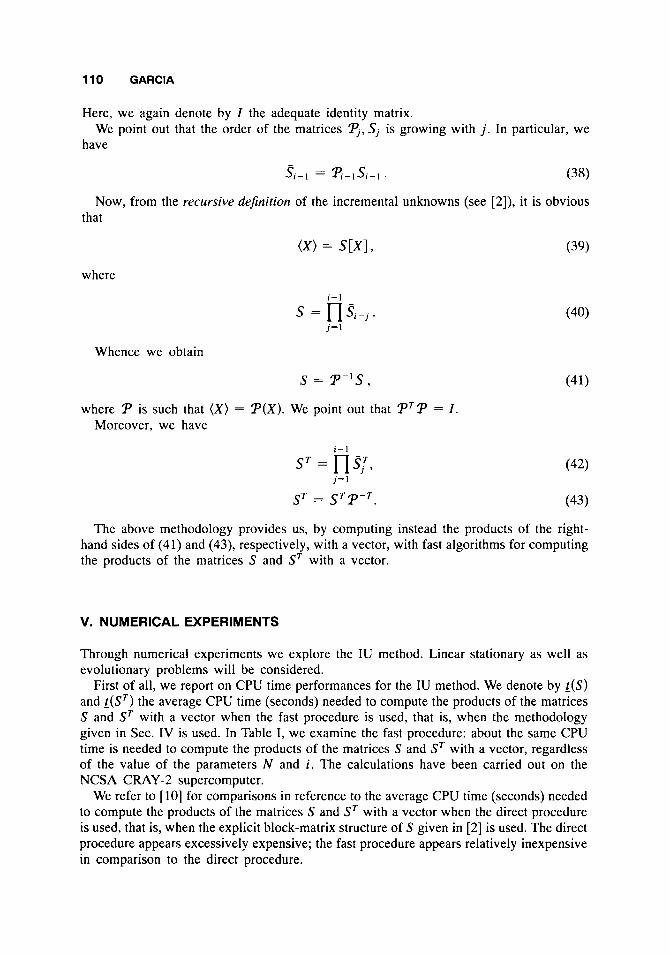
Here, we again denote by I the adequate identity matrix.
have We point out that the order of the matrices q, Sj is growing with j . In particular, we
Now, from the recursive definition of the incremental unknowns (see [2]), it is obvious that
where
Whence we obtain
(x) = S",
i-1
s = n S i P j . j = l
S = T ' S ,
Ve point out that F T F = where 33 is such that ( X ) = F(X) . Moreover, we have
(39)
The above methodology provides us, by computing instead the products of the right- hand sides of (41) and (43), respectively, with a vector, with fast algorithms for computing the products of the matrices S and ST with a vector.
V. NUMERICAL EXPERIMENTS
Through numerical experiments we explore the IU method. Linear stationary as well as evolutionary problems will be considered.
First of all, we report on CPU time performances for the IU method. We denote by t ( S ) and t ( S T ) the average CPU time (seconds) needed to compute the products of the matrices S and ST with a vector when the fast procedure is used, that is, when the methodology given in Sec. IV is used. In Table I, we examine the fast procedure: about the same CPU time is needed to compute the products of the matrices S and ST with a vector, regardless of the value of the parameters N and i . The calculations have been carried out on the NCSA CRAY-2 supercomputer.
We refer to [ 101 for comparisons in reference to the average CPU time (seconds) needed to compute the products of the matrices S and ST with a vector when the direct procedure is used, that is, when the explicit block-matrix structure of S given in [2] is used. The direct procedure appears excessively expensive; the fast procedure appears relatively inexpensive in comparison to the direct procedure.
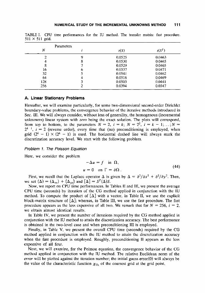
NUMERICAL STUDY OF THE INCREMENTAL UNKNOWNS METHOD 11 1
TABLE I. 511 X 511 grid.
CPU time performances for the IU method. The transfer matrix: fast procedure.
dST) Parameters
N 1 L(S)
2 9 0.0525 0.0463 4 8 0.0530 0.0465 8 7 0.0529 0.0465
16 6 0.0537 0.0471 32 5 0.0541 0.0462 64 4 0.0516 0.0469
128 3 0.0503 0.0441 256 2 0.0394 0.0347
A. Linear Stationary Problems
Hereafter, we will examine particularly, for some two-dimensional second-order Dirichlet boundary-value problems, the convergence behavior of the iterative methods introduced in Sec. 111. We will always consider, without loss of generality, the homogenous (incremental unknowns) linear system with zero being the exact solution. The plots will correspond, from top to bottom, to the parameters N = 2, i = k ; N = 22, i = k - l ; . . . ; N =
2 k - ' , i = 2 (reverse order), every time that (no) preconditioning is employed, when grid (2k - 1) X (2k - 1) is used. The horizontal dashed line will always mark the discretization accuracy level. We start with the following problem.
Problem 1 . The Poisson Equation
Here, we consider the problem - A u = f in R ,
u = O o n r = d R . (44)
First, we recall that the Laplace operator A is given by A = d ,'ax + d2/dy2. Then, we set (A) = ( A x x ) + (Ayy) and [A] = S T ( A ) S .
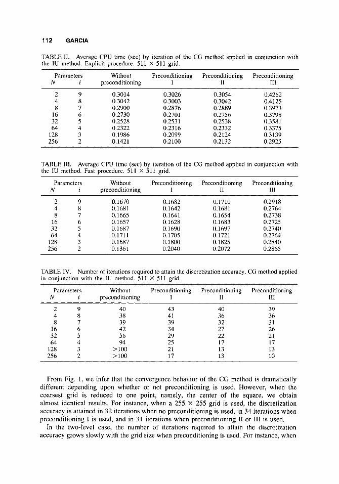
Now, we report on CPU time performances. In Tables I1 and 111, we present the average CPU time (seconds) by iteration of the CG method applied in conjunction with the IU method. To compute the product of [A] with a vector, in Table 11, we use the explicit block-matrix structure of [A]; whereas, in Table 111, we use the fast procedure. The fast procedure appears as the less expensive of all two. We remark that for N = 256, i = 2, we obtain almost identical results.
In Table IV, we present the number of iterations required by the CG method applied in conjunction with the IU method to attain the discretization accuracy. The best performance is obtained in the two-level case and when preconditioning I11 is employed.
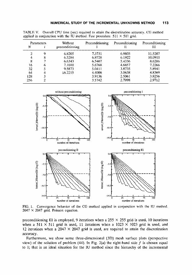
Finally, in Table V, we present the overall CPU time (seconds) required by the CG method applied in conjunction with the IU method to attain the discretization accuracy when the fast procedure is employed. Roughly, preconditioning I1 appears as the less expensive of all four.
Next, we will examine, for the Poisson equation, the convergence behavior of the CG method applied in conjunction with the IU method. The relative Euclidean norm of the error will be plotted against the iteration number; the initial guess error(0) will always be the value of the characteristic function XG,, of the coarsest grid at the grid point.
112 GARCIA
TABLE 11. the IU method. Explicit procedure. 51 1 X 51 1 grid.
Average CPU time (sec) by iteration of the CG method applied in conjunction with
Parameters Without Preconditioning Preconditioning Preconditioning N i preconditioning I I1 i11
2 9 4 8 8 7
16 6 32 5 64 4
128 3 256 2
0.3014 0.3042 0.2900 0.2730 0.2528 0.2322 0.1986 0.1421
0.3026 0.3003 0.2876 0.2701 0.2531 0.2316 0.2099 0.2100
0.3054 0.3042 0.2889 0.2756 0.2538 0.2332 0.2124 0.2132
0.4262 0.4125 0.3973 0.3798 0.3581 0.3375 0.3139 0.2925
TABLE 111. the IU method. Fast procedure. 51 1 X 51 1 grid.
Average CPU time (sec) by iteration of the CG method applied in conjunction with
Parameters Without Preconditioning Preconditioning Preconditioning N i preconditioning I I1 111
2 9 4 8 8 7
16 6 32 5 64 4
128 3 256 2
0.1670 0.1681 0.1665 0.1657 0.1687 0.1711 0.1687 0.1361
0.1682 0.1642 0.1641 0.1628 0.1690 0.1705 0.1800 0.2040
0.1710 0.1681 0.1654 0.1683 0.1697 0.1721 0.1825 0.2072
0.2918 0.2764 0.2738 0.2725 0.2740 0.2764 0.2840 0.2865
TABLE IV. in conjunction with the IU method. 51 1 X 51 1 grid.
Number of iterations required to attain the discrctization accuracy. CG method applied
Parameters Without Preconditioning Preconditioning Preconditioning N i preconditioning I I1 111
2 9 4 8 8 7
16 6 32 5 64 4
128 3 256 2
40 38 39 42 56 94
>I00 >loo
43 41 39 34 29 25 21 17
40 36 32 27 22 17 13 13
39 36 31 26 21 17 13 10
From Fig. 1, we infer that the convergence behavior of the CG method is dramatically different depending upon whether or not preconditioning is used. However, when the coarsest grid is reduced to one point, namely, the center of the square, we obtain almost identical results. For instance, when a 255 X 255 grid is used, the discretization accuracy is attained in 32 iterations when no preconditioning is used, in 34 iterations when preconditioning I is used, and in 31 iterations when preconditioning I1 or I11 is used.
In the two-level case, the number of iterations required to attain the discretization accuracy grows slowly with the grid size when preconditioning is used. For instance, when
NUMERICAL STUDY OF THE INCREMENTAL UNKNOWNS METHOD 11 3
TABLE V. applied in conjunction with the IU method. Fast procedure. 511 X 511 grid.
Overall CPU time (sec) required to attain the discretization accuracy. CG method
Parameters Without Preconditioning Preconditioning Preconditioning N i preconditioning I I1 I11
2 9 6.8205 4 8 6.5284 8 7 6.6343
16 6 7.1010 32 5 9.5873 64 4 16.2215
128 3 256 2
7.3731 6.8728 6.5407 5.6768 5.041 1 4.4006 3.9136 3.5742
6.9805 6.1922 5.4336 4.6857 3.8735 3.0638 2.5061 2.7998
11.5207 10.0910 8.6286 7.2266 5.8941 4.8369 3.8256 2.9712
without preconditioning preconditioning I
-14.0 !-I 25 50 75 loo number of iterations
-14.0 25 so 75 100 number of iterations
preconditioning 11 preconditioning 111 0.0 0.0
o "M -3.5 o 7" -3.5
0, o_
s
0 0 c v h - -
h
6 -7.0 8 -7.0
5 ? 5 ? 5
- 9 -10.5 - 5 -Ios
v v
8 6
-14.01 n I s I . I s 1 0 25 M 75 loo
number of iterations
-14.0- 0 25 50 75 100
number of iterations
FIG. 1. 2047 X 2047 grid. Poisson equation.
Convergence behavior of the CG method applied in conjunction with the IU method.
preconditioning 111 is employed, 9 iterations when a 255 X 255 grid is used, 10 iterations when a 511 X 511 grid is used, 11 iterations when a 1023 X 1023 grid is used, and 12 iterations when a 2047 X 2047 grid is used, are required to attain the discretization accuracy.
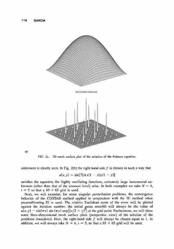
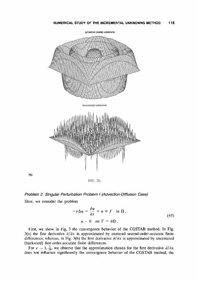
Furthermore, we show some three-dimensional (3D) mesh surface plots (perspective view) of the solution of problem (44). In Fig. 2(a) the right-hand side f is chosen equal to 1; that is an ideal situation for the IU method since the hierarchy of the incremental
114 GARCIA
(a)
FIG. 2a. 3D mesh surface plot of the solution of the Poisson equation.
unknowns is clearly seen. In Fig. 2(b) the right-hand side f is chosen in such a way that
u ( x , y ) = sin[72rx(l - x ) y ( I - y ) ]
satisfies the equation; for highly oscillating functions, extremely large incremental un- knowns (other than that of the coarsest level) arise. In both examples we take N = 4, i = 5 so that a 65 X 65 grid is used.
Next, we will examine, for some singular perturbation problems, the convergence behavior of the CGSTAB method applied in conjunction with the IU method when preconditioning I11 is used. The relative Euclidean norm of the error will be plotted against the iteration number; the initial fuess error(0) will always be the value of u ( x , y ) = sin(nx) sin ( r y ) exp[(x/2 + y) ] at the grid point. Furthermore, we will show some three-dimensional mesh surface plots (perspective view) of the solution of the problems considered. Here, the right-hand side f will always be chosen equal to 1. In addition, we will always take N = 4, i = 5, so that a 65 X 65 grid will be used.
NUMERICAL STUDY OF THE INCREMENTAL UNKNOWNS METHOD 115
primitive (nodal) unknowns
FIG. 2b.
Problem 2. Singular Perturbation Problem I (Advecrion-Diffusion Case)
Here, we consider the problem
au a x
-vAu + - + u = f in a , u = O o n r = d R .
(45)
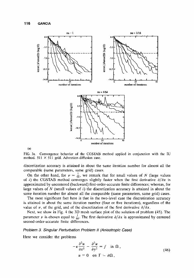
First, we show in Fig. 3 the convergence behavior of the CGSTAB method. In Fig. 3(a) the first derivative a/ax is approximated by centered second-order-accurate finite differences; whereas, in Fig. 3(b) the first derivative d/ax is approximated by uncentered (backward) first-order-accurate finite differences.
For v = 1, 16, we observe that the approximation chosen for the first derivative a/ax does not influence significantly the convergence behavior of the CGSTAB method, the
I
116 GARCIA
nu = 1 nu = 1/16 0.0 0.0
s h 3 -3.5 “M -3.5 0 - v - 8
E! 3
- s 6
1 -7’0
-7.0
-? v v : -10.5 1 -10.5 * *
-14.0 -14.0 0 25 50 0 25 50
number of iterations number of iterations
nu = 1/64 0.0
s “M -3.5
o
0 - v - -7.0
5 c
g -10.5 3!
-14.0- 25 50
number of iterations
(a)
FIG. 3a. method. 51 1 X 51 1 grid. Advection-diffusion case.
discretization accuracy is attained in about the same iteration number for almost all the comparable (same parameters, same grid) cases.
On the other hand, for v = 64, we remark that for small values of N (large values of i) the CGSTAB method converges slightly faster when the first derivative a/dx is approximated by uncentered (backward) first-order-accurate finite differences; whereas, for large values of N (small values of i) the discretization accuracy is attained in about the same iteration number for almost all the comparable (same parameters, same grid) cases.
The most significant fact here is that in the two-level case the discretization accuracy is attained in about the same iteration number (four or five iterations), regardless of the value of v, of the grid, and of the discretization of the first derivative a/ax.
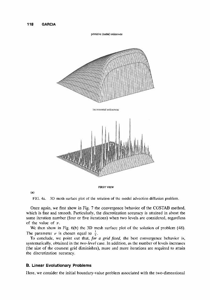
Next, we show in Fig. 4 the 3D mesh surface plot of the solution of problem (45). The parameter v is chosen equal to 64. The first derivative a/dx is approximated by centered second-order-accurate finite differences.
Convergence behavior of the CGSTAB method applied in conjunction with the IU
1
1
Problem 3. Singular Perturbation Problem II (Anisotropic Case)
Here we consider the problems
U = O o n r = a R ,
NUMERICAL STUDY OF THE INCREMENTAL UNKNOWNS METHOD 117
(W
and
nu = I nu = 1/16 0.0 0.0
- 0 -3.5 8 -3.5
2 e ' -7.0
r
- 8
5
- o
i -7.0
5 r: 2 a 22 - v
p -10.5 8
-10.5
-14.0 -14.0 0 2 5 50 0 2 5 5 0
number of iterations number of iterations
nu = 1/64
-14.01 . I . I . I I 1 25 50
number of iterations
FIG. 3b.
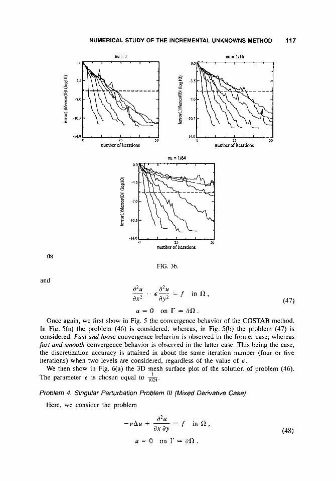
u = O o n r = d R . Once again, we first show in Fig. 5 the convergence behavior of the CGSTAB method.
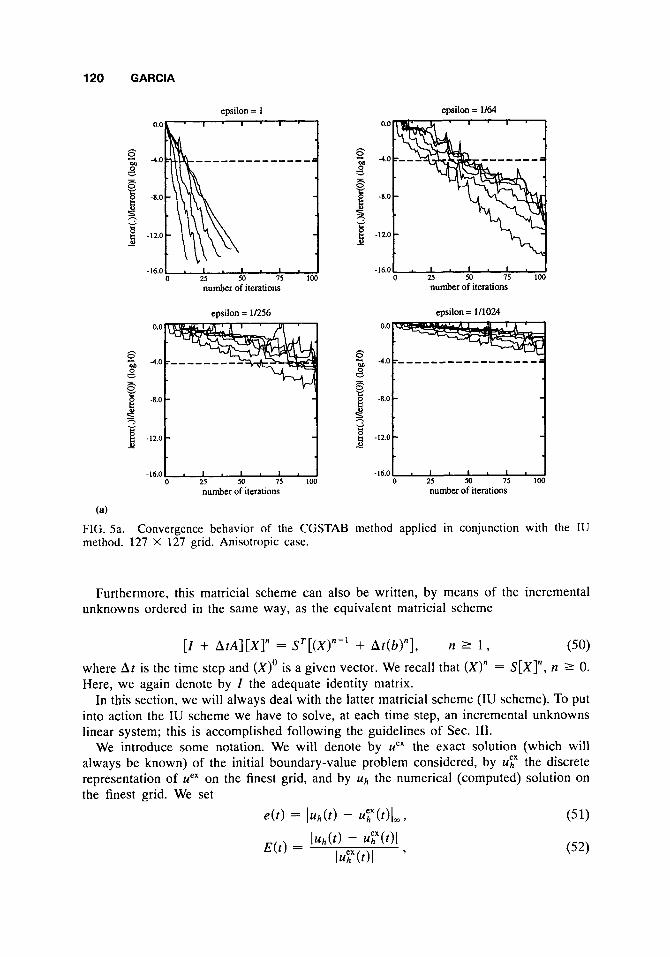
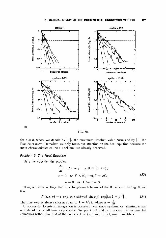
In Fig. 5(a) the problem (46) is considered; whereas, in Fig. 5(b) the problem (47) is considered. Fast and loose convergence behavior is observed in the former case; whereas fast and smooth convergence behavior is observed in the latter case. This being the case, the discretization accuracy is attained in about the same iteration number (four or five iterations) when two levels are considered, regardless of the value of E .
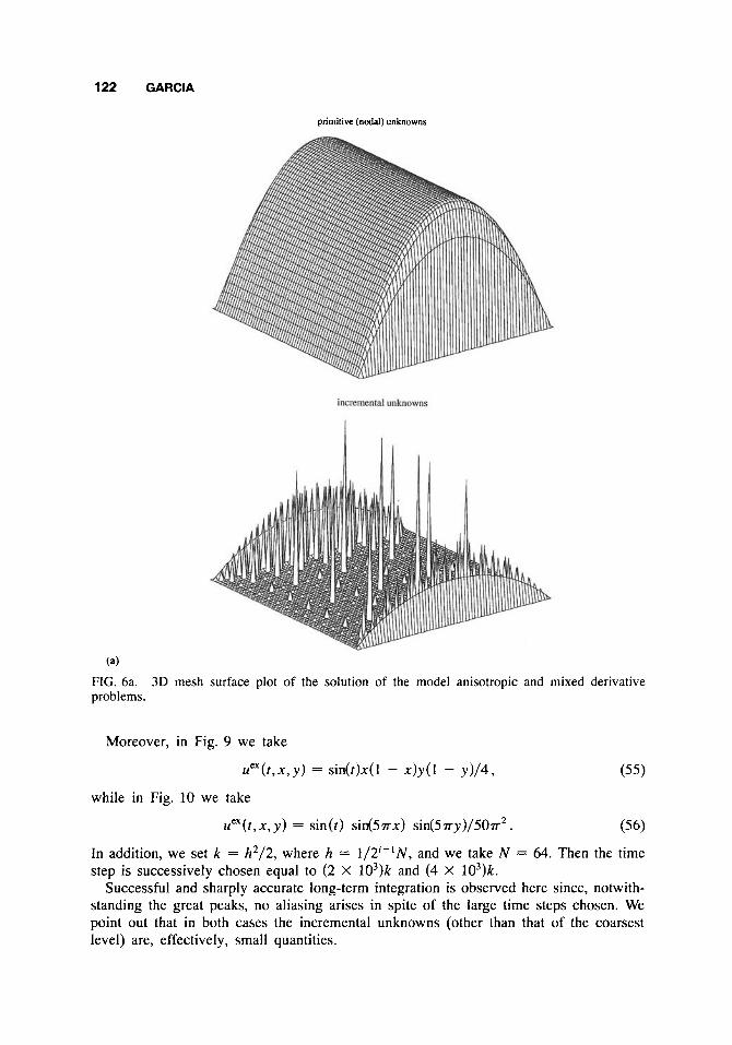
We then show in Fig. 6(a) the 3D mesh surface plot of the solution of problem (46). The parameter E is chosen equal to 1024. 1
Problem 4. Singular Perturbation Problem 111 (Mixed Derivative Case)
Here, we consider the problem
a2u ax ay
- V A U + ~ = f i n R ,
u = O o n r = a R .
118 GARCIA
primitive (nodal) unknowns
FIRST VIEW
(a)
FIG. 4a. 3D mesh surface plot of the solution of the model advection-diffusion problem.
Once again, we first show in Fig. 7 the convergence behavior of the CGSTAB method, which is fast and smooth. Particularly, the discretization accuracy is attained in about the same iteration number (four or five iterations) when two levels are considered, regardless of the value of Y.
We then show in Fig. 6(b) the 3D mesh surface plot of the solution of problem (48). The parameter Y is chosen equal to 1.
To conclude, we point out that, for a grid jixed, the best convergence behavior is, systematically, obtained in the two-level case. In addition, as the number of levels increases (the size of the coarsest grid diminishes), more and more iterations are required to attain the discretization accuracy.
1
B. Linear Evolutionary Problems
Here, we consider the initial boundary-value problem associated with the two-dimensional
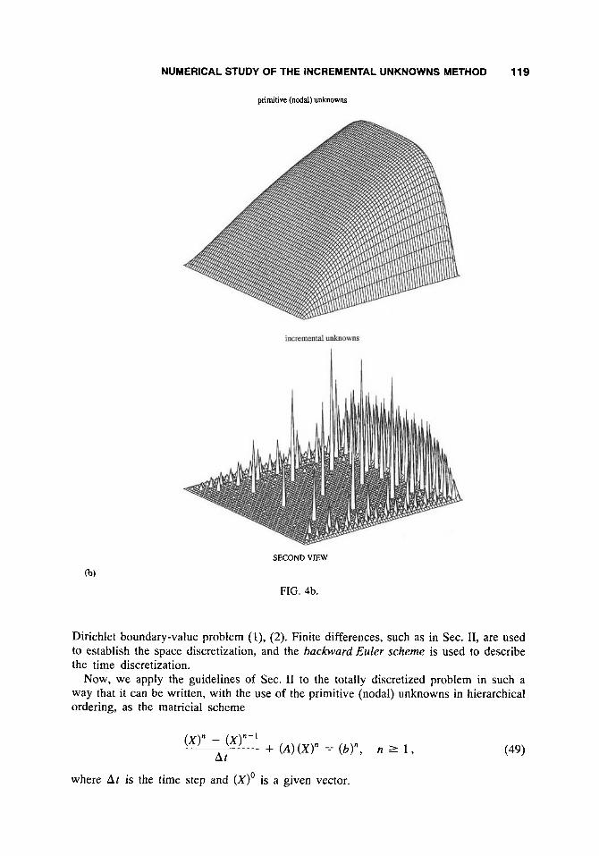
NUMERICAL STUDY OF THE INCREMENTAL UNKNOWNS METHOD 119
primitive (nodal) unknowns
SECOND VIEW
FIG. 4b.
Dirichlet boundary-value problem (l), (2). Finite differences, such as in Sec. 11, are used to establish the space discretization, and the backward Euler scheme is used to describe the time discretization.
Now, we apply the guidelines of Sec. 11 to the totally discretized problem in such a way that it can be written, with the use of the primitive (nodal) unknowns in hierarchical ordering, as the matricial scheme
( X ) " - (x)"-* + (A) (X)" = (b)" , n 2 1 , At (49)
where A t is the time step and (XIo is a given vector.
120 GARCIA
epsilon = 1 epsilon = 1/64 0.0 0.0
o -4.0
6 4.0
8 - 8 -
8 8 E -120 9 -120
5 c v
Y -
-16.0 -16.0 0 2.5 50 75 100 0 25 50 75 100
number of iterations
epsilon = 1R56
number of iterations
epsilon = lll02.4
0 25 50 75 100 0 25 50 75 100 number of iterations number of iterations
(a)
FIG. 5a. method. 127 X 127 grid. Anisotropic case.
Convergence behavior of the CGSTAB method applied in conjunction with the IU
Furthermore, this matricial scheme can also be written, by means of the incremental unknowns ordered in the same way, as the equivalent matricial scheme
[ I + A t A ] [ X ] " = S'[(X)"-' + A t ( b ) " ] , n 2 1, (50) where Ar is the time step and (X)' is a given vector. We recall that (X)" = S [ X ] " , n 2 0. Here, we again denote by I the adequate identity matrix.
In this section, we will always deal with the latter matricial scheme (IU scheme). To put into action the IU scheme we have to solve, at each time step, an incremental unknowns linear system; this is accomplished following the guidelines of Sec. 111.
We introduce some notation. We will denote by uex the exact solution (which will always be known) of the initial boundary-value problem considered, by U? the discrete representation of uex on the finest grid, and by U h the numerical (computed) solution on the finest grid. We set
e ( t ) = I U h ( t ) - UY(r)lm, (51)
NUMERICAL STUDY OF THE INCREMENTAL UNKNOWNS METHOD 121
epsilon = 1 epsilon = 1/64 0.0 0.0
o
8 s o E -8.0 8
h
-4.0 “M 4.0 0 a - -
’E:
6 3 3 -12.0 1 -12.0 - 1y
-16.0 -16.0 0 25 50 7s 100 0 25 M 75 loo
number of iterations number of iterations
epsilon = 1 f i 6 epsilon = 111024 0.0 0.0
: -4.0 o 4.0
0 8 - - v - - 6 8
8 -8.0 1 8 - T c v
T v
g -120 g -120 32 32
-16.0 -16.0 0 50 7s loo 0 25 50 75 100
number of iterations number of iterations
(W FIG. 5b.
for t 2 0, where we denote by I . I m the maximum absolute value norm and by I * I the Euclidean norm. Hereafter, we only focus our attention on the heat equation because the main characteristics of the IU scheme are already observed.
Problem 5. The Heat Equation
Here we consider the problem du _ _ Au = f dt
u = 0
in fl X (0, +a),
on r x (0, +a), r = a f l , (53)
u = O i n f l f o r t = O . Now, we show in Figs. 8-10 the long-term behavior of the IU scheme. In Fig. 8, we
take
uex(t,x,y) = t exp( r t ) sin(rx) sin(ry) exp[(x/2 + y)’]. (54) 1 The time step is always chosen equal to k = h2/2, where h = 5.
Unsuccessful long-term integration is observed here since systematical aliasing arises in spite of the small time step chosen. We point out that in this case the incremental unknowns (other than that of the coarsest level) are not, in fact, small quantities.
122 GARCIA
primitive (nodal) unknowns
(a)
FIG. 6a. problems.
3D mesh surface plot of the solution of the model anisotropic and mixed derivative
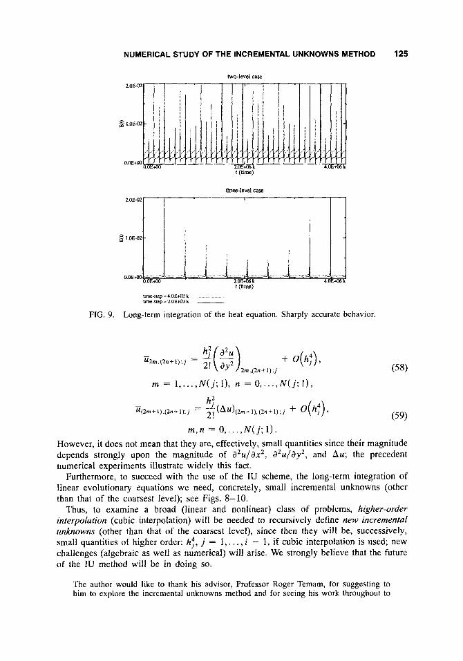
Moreover, in Fig. 9 we take
uex(t,x,y) = sin(t)x(l - x)y(l - y)/4,
uex(t,x,y) = sin(t) sin(5.rrx) sin(5.rry)/50.rr2.
(55)
while in Fig. 10 we take
(56)
In addition, we set k = h2/2 , where h = 1 / 2 ; - ' N , and we take N = 64. Then the time step is successively chosen equal to (2 X 10³)k and (4 X 10³)k.
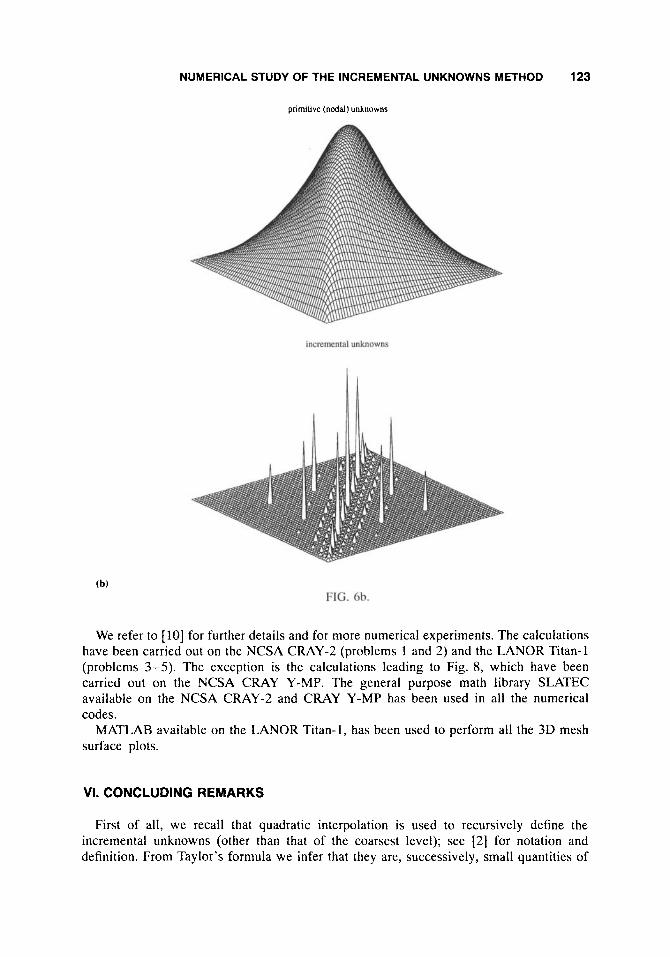
Successful and sharply accurate long-term integration is observed here since, notwith- standing the great peaks, no aliasing arises in spite of the large time steps chosen. We point out that in both cases the incremental unknowns (other than that of the coarsest level) are, effectively, small quantities.
NUMERICAL STUDY OF THE INCREMENTAL UNKNOWNS METHOD 123
primitive (nodal) unknowns
We refer to [ 101 for further details and for more numerical experiments. The calculations have been carried out on the NCSA CRAY-2 (problems 1 and 2) and the LANOR Titan-1 (problems 3-5). The exception is the calculations leading to Fig. 8, which have been carried out on the NCSA CRAY Y-MP. The general purpose math library SLATEC available on the NCSA CRAY-2 and CRAY Y-MP has been used in all the numerical codes.
MATLAB available on the LANOR Titan-1, has been used to perform all the 3D mesh surface plots.
VI. CONCLUDING REMARKS
First of all, we recall that quadratic interpolation is used to recursively define the incremental unknowns (other than that of the coarsest level); see [2] for notation and definition. From Taylor’s formula we infer that they are, successively, small quantities of
124 GARCIA
nu = 1 nu=2f3
-16.01 * I * I . I . I 0 25 50 75 loo
number of iterations
nu = 8/15
-16.01 * I * I s I . 1 0 25 50 75 loo
number of iterations
-16.0- 25 50 75 loo number of iterations
nu = In
0 25 50 75 loo number of iterations
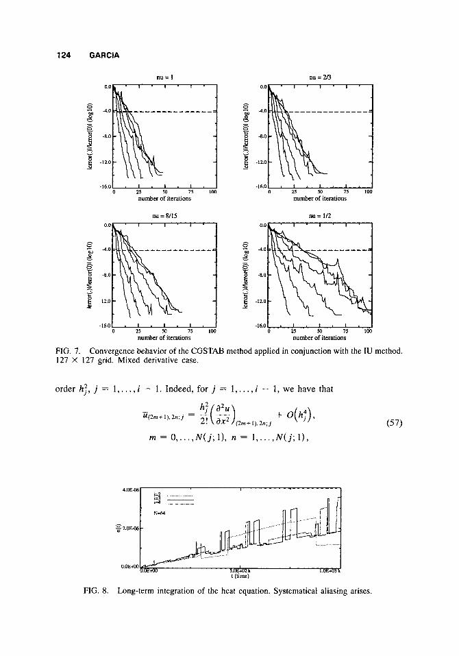
FIG. 7. 127 X 127 grid. Mixed derivative case.
Convergence behavior of the CGSTAB method applied in conjunction with the IU method.
order h;, j = 1,. . .,i - 1. Indeed, for j = 1,. . . , i - 1, we have that
m = 0 ..... N ( j ; l ) , n = 1 ..... N ( j ; l ) ,
4.0E-06 I 1=2 . . . . . . . . . . . 1=3 -
?-. 3 2.0E-06 - ..........
j !
.................
FIG. 8. Long-term integration of the heat equation. Systematical aliasing arises.
NUMERICAL STUDY OF THE INCREMENTAL UNKNOWNS METHOD 125
2 . O E M
O.OEt00
two-level case
I (time)
threelevel case
umc-rep = 4 OEt03 k urn step = 2 OE43 k __
FIG. 9. Long-term integration of the heat equation. Sharply accurate behavior.
m = I , . . . ,N (J ; I) , n = 0,. . . , N ( J ; I ) ,
m , n = 0,. . . ,N (J ; 1). However, it does not mean that they are, effectively, small quantities since their magnitude depends strongly upon the magnitude of a2u/ax2, d2u/dy2, and A M ; the precedent numerical experiments illustrate widely this fact.
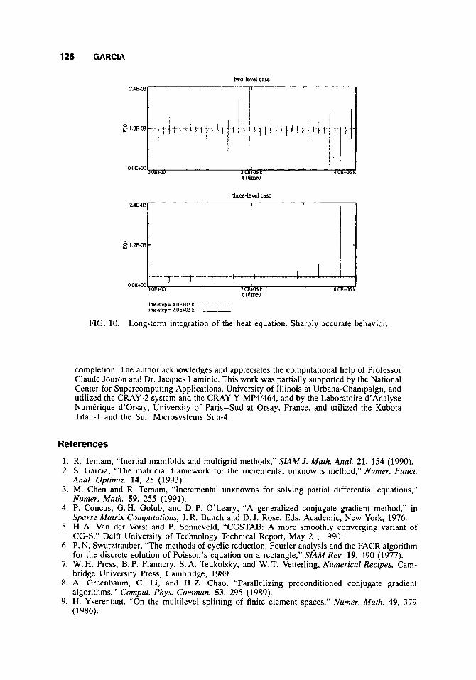
Furthermore, to succeed with the use of the IU scheme, the long-term integration of linear evolutionary equations we need, concretely, small incremental unknowns (other than that of the coarsest level); see Figs. 8-10.
Thus, to examine a broad (linear and nonlinear) class of problems, higher-order interpolation (cubic interpolation) will be needed to recursively define new incremental unknowns (other than that of the coarsest level), since then they will be, successively, small quantities of higher order: h;, j = 1,. , . , i - 1, if cubic interpolation is used; new challenges (algebraic as well as numerical) will arise. We strongly believe that the future of the IU method will be in doing so.
The author would like to thank his advisor, Professor Roger Temam, for suggesting to him to explore the incremental unknowns method and for seeing his work throughout to
126 GARCIA
two-level case
I O.OE*OO I 2.0Eto6 k 4 . 0 E 4 t (time)
three-level case I
I 2.4E03
O.OE*OO 2.OEto6 k 4.0E& 1 (time)
limc-skp=4.0E+03 k __...._.._.._.... Um-slcp = 2OE+O3 k ~
FIG. 10. Long-term integration of the heat equation. Sharply accurate behavior.
completion. The author acknowledges and appreciates the computational help of Professor Claude Jouron and Dr. Jacques Laminie. This work was partially supported by the National Center for Supercomputing Applications, University of Illinois at Urbana-Champaign, and utilized the CRAY-2 system and the CRAY Y-MP4/464, and by the Laboratoire d’Analyse NumCrique d’Orsay, University of Paris-Sud at Orsay, France, and utilized the Kubota Titan-1 and the Sun Microsystems Sun-4.
References
1. R. Temam, “Inertial manifolds and multigrid methods,” SZAM J . Math. Anal. 21, 154 (1990). 2. S. Garcia, “The matricial framework for the incremental unknowns method,” Numer. Funct.
Anal. Optimiz. 14, 25 (1993). 3. M. Chen and R. Temam, “Incremental unknowns for solving partial differential equations,”
Numer. Math. 59, 255 (1991). 4. P. Concus, G. H. Golub, and D. P. O’Leary, “A generalized conjugate gradient method,” in
Sparse Matrix Computations, J. R. Bunch and D. J. Rose, Eds. Academic, New York, 1976. 5. H.A. Van der Vorst and P. Sonneveld, “CGSTAB: A more smoothly converging variant of
CG-S,” Delft University of Technology Technical Report, May 21, 1990. 6. P. N. Swarztrauber, “The methods of cyclic reduction, Fourier analysis and the FACR algorithm
for the discrete solution of Poisson’s equation on a rectangle,” SIAM Rev. 19, 490 (1977). 7. W. H. Press, B. P. Flannery, S. A. Teukolsky, and W. T. Vetterling, Numerical Recipes, Cam-
bridge University Press, Cambridge, 1989. 8. A. Greenbaum, C . Li, and H. Z. Chao, “Parallelizing preconditioned conjugate gradient
algorithms,” Comput. Phys. Commun. 53, 295 (1989). 9. H. Yserentant, “On the multilevel splitting of finite element spaces,” Numer. Math. 49, 379
(1986).
NUMERICAL STUDY OF THE INCREMENTAL UNKNOWNS METHOD 127
10. S. Garcia, “Numerical study of the incremental unknowns method,” UniversitC de Paris-Sud, MathCmatiques, Report No. 49, 1992.
11. 0. Axelsson and I. Gustafsson, “A modified upwind scheme for convective transport equations and the use of a conjugate gradient method for the solution of non-symmetric systems of equations,” J. Inst. Math. Appl., 23, 321 (1979).
12. R. E. Bank, T. F. Dupont, and H. Yserentant, “The hierarchical basis multigrid method,” Numer. Math. 52, 427 (1988).
13. G. Brussino and V. Sonnad, “A comparison of direct and preconditioned iterative techniques for sparse, unsymmetric systems of linear equations,” Int. J. Numer. Methods Eng., 28, 801 (1989).
14. W. Hackbush, Multigrid Methods and Applications, Springer-Verlag, Berlin, 1985. 15. R. Peyret and T. D. Taylor, Computational Methods for Fluid Flow, Springer-Verlag, Berlin,
16. H.A. Van der Vorst, “Iterative solution methods for certain sparse linear systems with a
17. R. L. Lynch, J. R. Rice, and D. H. Thomas, “Direct solution of partial difference equations by
18. B. F. Smith and 0. B. Widlund, “A domain decomposition algorithm using a hierarchical basis,’’
1983.
non-symmetric matrix arising from PDE problems,” J. Comput. Phys. 44, 1 (1981).
tensor product methods,” Numer. Math. 6 , 185 (1964).
SIAM J. Sci. Stat. Comput. 11, 1212 (1990).