Adaptive Critic Based Optimal Kinematic Control for a Robot ...
Upload
khangminh22Category
view
2download
0
Adaptive Control – Landau,Lozano, M’Saad, Karimi1
Adaptive Control
Chapter 7: Digital Control Strategies
Adaptive Control – Landau,Lozano, M’Saad, Karimi2
Chapter 7:Digital Control Strategies
Adaptive Control – Landau,Lozano, M’Saad, Karimi3
r(t)
m
m
AB
TS1
ABq d−
R
u(t) y(t)
Controller
PlantModel
+
-
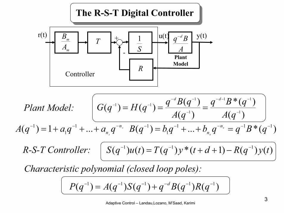
The R-S-T Digital Controller
Plant Model:)(
)(*)(
)()()(1
11
1
111
−
−−−
−
−−−− ===
qAqBq
qAqBqqHqG
dd
A
A
nn qaqaqA −−− +++= ...1)( 1
11 )(*...)( 111
11 −−−−− =++= qBqqbqbqB B
B
nn
R-S-T Controller: )()()1(*)()()( 111 tyqRdtyqTtuqS −−− −++=
Characteristic polynomial (closed loop poles):
)()()()()( 11111 −−−−−− += qRqBqqSqAqP d
Adaptive Control – Landau,Lozano, M’Saad, Karimi4
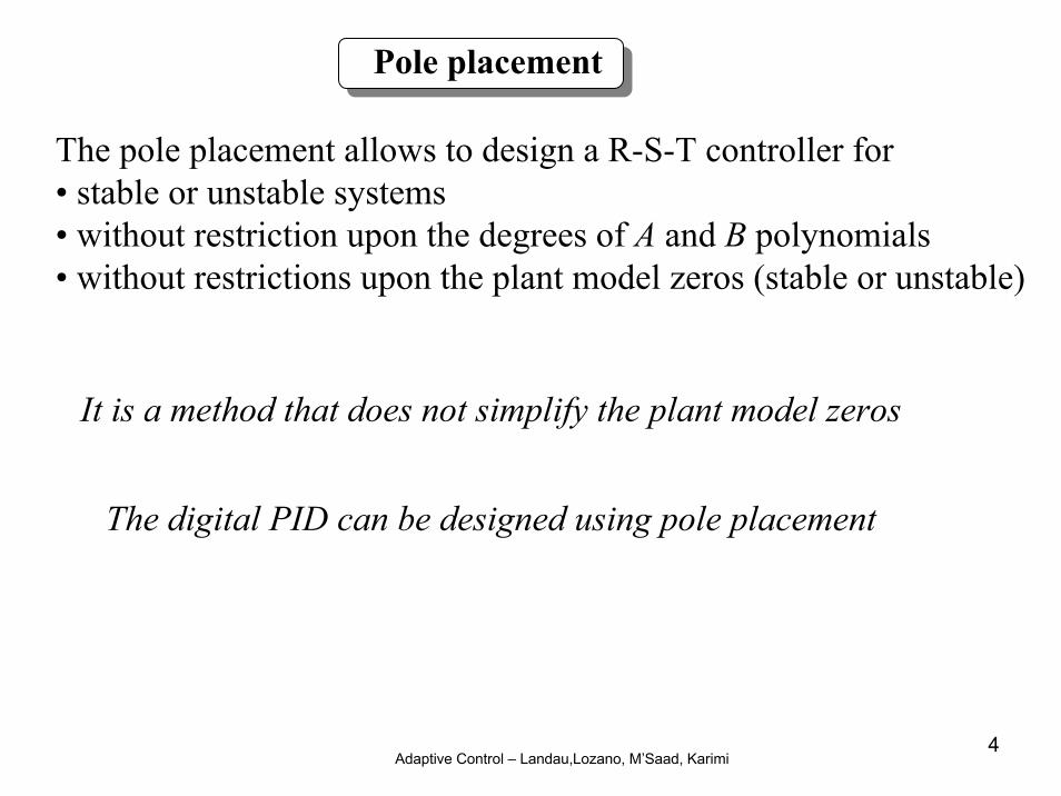
Pole placement
It is a method that does not simplify the plant model zeros
The pole placement allows to design a R-S-T controller for• stable or unstable systems• without restriction upon the degrees of A and B polynomials• without restrictions upon the plant model zeros (stable or unstable)
The digital PID can be designed using pole placement
Adaptive Control – Landau,Lozano, M’Saad, Karimi5
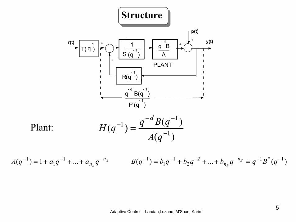
Structure
)()()( 1
11
−
−−− =
qAqBqqH
d
AA
nn qaqaqA −−− +++= ...1)( 1
11 )(...)( 1*12
21
11 −−−−−− =+++= qBqqbqbqbqB B
B
nn
Plant:
) ------------1
(q- 1
)---------q
- dB
A
PLANT
R(q- 1
)
--------------------q
- dB(q
- 1)
(q- 1
)
S
P
r(t) y(t)+
-
T( ) q - 1
p(t)
++

Adaptive Control – Landau,Lozano, M’Saad, Karimi6
)()()(
)()()()()()()( 1
11
1111
111
−
−−−
−−−−−
−−−− =
+=
qPqBqTq
qRqBqqSqAqBqTqqH
d
d
d
BF
....1)()()()()( 22
11
11111 +++=+= −−−−−−−− qpqpqRqBqqSqAqP d
)()()(
)()()()()()()(
1
11
1111
111
−
−−
−−−−−
−−− =
+=
qPqSqA
qRqBqqSqAqSqAqS
dyp
Closed loop T.F. (r y) (reference tracking)
Defines the (desired )closed loop poles
Closed loop T.F. (p y) (disturbance rejection)
Output sensitivity function
Pole placement

Adaptive Control – Landau,Lozano, M’Saad, Karimi7
Choice of desired closed loop poles (polynomial P)
)()()( 111 −−− = qPqPqP FD
Dominant poles Auxiliary poles
Specificationin continuous time(tM, M)
2nd order (ω0, ζ)discretization
eT )( 1−qPD
5.125.0 0 ≤≤ eTω17.0 ≤≤ ζ
Choice of PD(q-1)(dominant poles)
• Auxiliary poles are introduced for robustness purposes• They usually are selected to be faster than the dominant poles
Auxiliary poles
Adaptive Control – Landau,Lozano, M’Saad, Karimi8
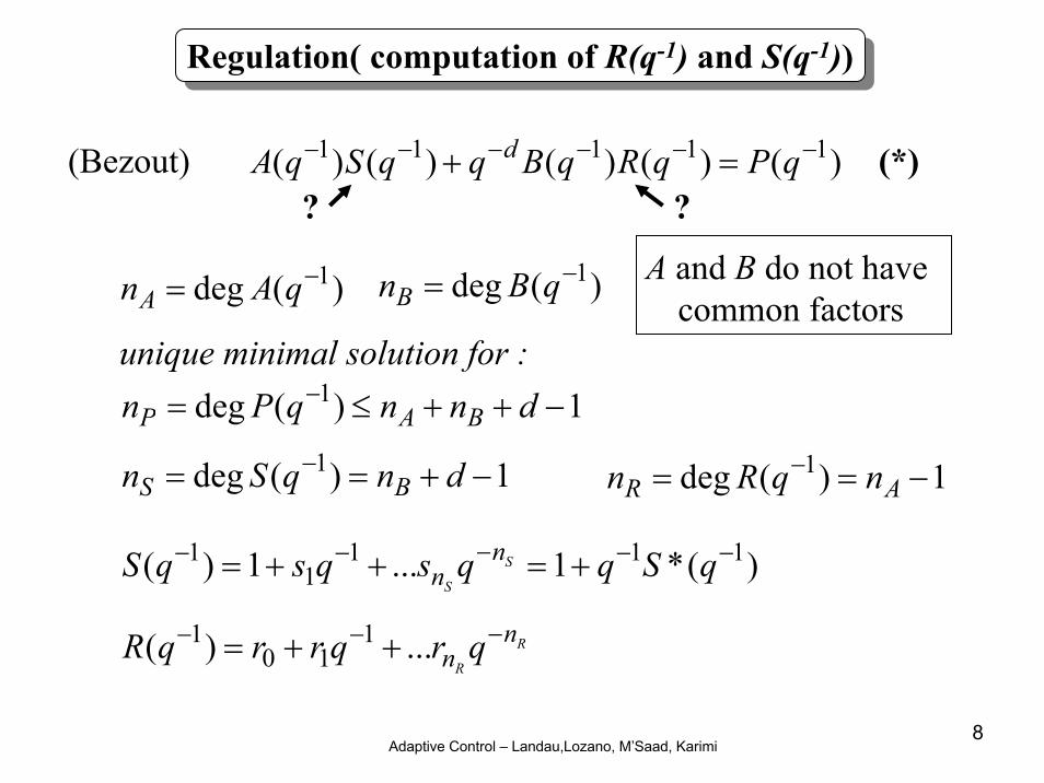
Regulation( computation of R(q-1) and S(q-1))
)()()()()( 11111 −−−−−− =+ qPqRqBqqSqA d
? ?
)(deg 1−= qAnA )(deg 1−= qBnBA and B do not have
common factors
(Bezout)
unique minimal solution for :1)(deg 1 −++≤= − dnnqPn BAP
1)(deg 1 −+== − dnqSn BS 1)(deg 1 −== −AR nqRn
)(*1...1)( 1111
1 −−−−− +=++= qSqqsqsqS S
S
nn
R
R
nn qrqrrqR −−− ++= ...)( 1
101
(*)
Adaptive Control – Landau,Lozano, M’Saad, Karimi9
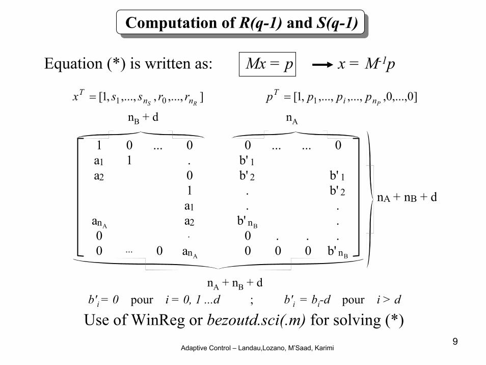
Computation of R(q-1) and S(q-1)
Equation (*) is written as: Mx = p
],...,,,...,,1[ 01 RS nnT rrssx = ]0,...,0,,...,,...,,1[ 1 Pni
T pppp =
1 0 ... 0a1 1 .a2 0
1a1
anA a20 .
0 ... 0 anA
0 ... ... 0b' 1b' 2 b' 1. b' 2. .
b' nB .0 . . .0 0 0 b' nB
nA + nB + d
nB + d nA
nA + nB + d
x = M-1p
Use of WinReg or bezoutd.sci(.m) for solving (*)b'i = 0 pour i = 0, 1 ...d ; b'i = bi-d pour i > d
Adaptive Control – Landau,Lozano, M’Saad, Karimi10
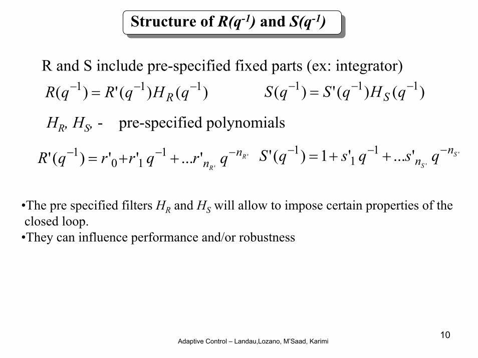
Structure of R(q-1) and S(q-1)
R and S include pre-specified fixed parts (ex: integrator)
)()(')( 111 −−− = qHqRqR R )()(')( 111 −−− = qHqSqS S
HR, HS, - pre-specified polynomials
'
''...'')(' 1
101 R
R
nn qrqrrqR −−− ++= '
''...'1)(' 1
11 S
S
nn qsqsqS −−− ++=
•The pre specified filters HR and HS will allow to impose certain properties of the closed loop.•They can influence performance and/or robustness
Adaptive Control – Landau,Lozano, M’Saad, Karimi11
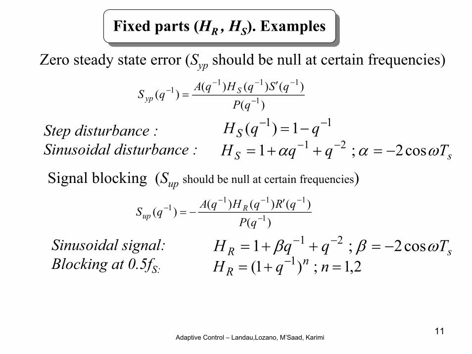
Fixed parts (HR , HS). Examples
Zero steady state error (Syp should be null at certain frequencies)
Step disturbance : Sinusoidal disturbance : sS TqqH ωαα cos2;1 21 −=++= −−
11 1)( −− −= qqHS
Signal blocking (Sup should be null at certain frequencies)
sR TqqH ωββ cos2;1 21 −=++= −−
2,1;)1( 1 =+=Sinusoidal signal:Blocking at 0.5fS:
− nqH nR
)()()()(
)( 1
1111
−
−−−− ′
=qP
qSqHqAqS S
yp
)()()()()( 1
1111
−
−−−− ′
−=qP
qRqHqAqS Rup
Adaptive Control – Landau,Lozano, M’Saad, Karimi12
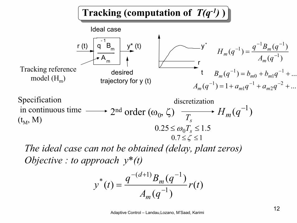
Tracking (computation of T(q-1) )
------------q
- 1Bm
Am
Ideal case
r (t) y* (t)
desiredtrajectory for y (t)
t
y
r
*
Tracking referencemodel (Hm)
2nd order (ω0, ζ)discretization
sT )( 1−qHm
5.125.0 0 ≤≤ sTω17.0 ≤≤ ζ
)()(
)( 1
111
−
−−− =
qAqBq
qHm
mm
The ideal case can not be obtained (delay, plant zeros)Objective : to approach y*(t)
)()(
)()( 1
1)1(* tr
qAqBq
tym
md
−
−+−
=
...)( 110
1 ++= −− qbbqB mmm
...1)( 22
11
1 +++= −−− qaqaqA mmm
Specificationin continuous time(tM, M)
Adaptive Control – Landau,Lozano, M’Saad, Karimi13
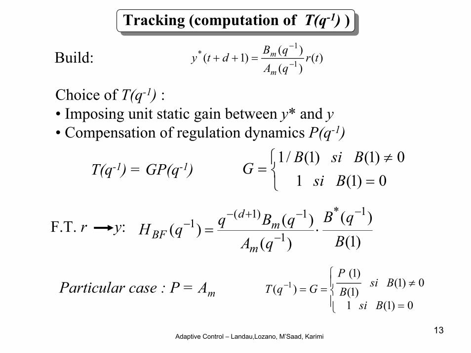
)()()(
)1( 1
1* tr
qAqB
dtym
m−
−
=++Build:
Choice of T(q-1) :• Imposing unit static gain between y* and y• Compensation of regulation dynamics P(q-1)
⎩⎨⎧
=≠
=0)1(1
0)1()1(/1Bsi
BsiBGT(q-1) = GP(q-1)
Particular case : P = Am⎪⎩
⎪⎨⎧
=
≠==−
0)1(1
0)1()1()1(
)( 1
Bsi
BsiBP
GqT
F.T. r y:)1(
)(
)()()(
1*
1
1)1(1
BqB
qAqBqqH
m
md
BF
−
−
−+−− ⋅=
Tracking (computation of T(q-1) )

Adaptive Control – Landau,Lozano, M’Saad, Karimi14
Pole placement. Tracking and regulation
+
-
R
1 q-d
BAS
TA
Bm
m
r(t)
y (t+d+1)*u(t) y(t)
q
-(d+1)
P(q -1 )q
-(d+1)
B*(q )-1
B*(q )
-1
B(1)q
-(d+1) B m(q )
B*(q )
-1-1
A m(q ) B(1)-1
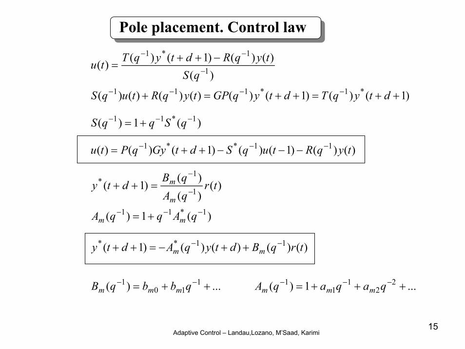
)1(*)()()()()( 111 ++=+ −−− dtyqTtyqRtuqS
Adaptive Control – Landau,Lozano, M’Saad, Karimi15
)()()()1()()( 1
1*1
−
−− −++=
qStyqRdtyqTtu
)1()()1()()()()()( *1*111 ++=++=+ −−−− dtyqTdtyqGPtyqRtuqS
)(1)( 1*11 −−− += qSqqS
)()()1()()1()()( 11**1 tyqRtuqSdtGyqPtu −−− −−−++=
)()()(
)1( 1
1* tr
qAqB
dtym
m−
−
=++
)(1)( 1*11 −−− += qAqqA mm
)()()()()1( 11** trqBdtyqAdty mm−− ++−=++
...)( 110
1 ++= −− qbbqB mmm ...1)( 22
11
1 +++= −−− qaqaqA mmm
Pole placement. Control law
Adaptive Control – Landau,Lozano, M’Saad, Karimi16
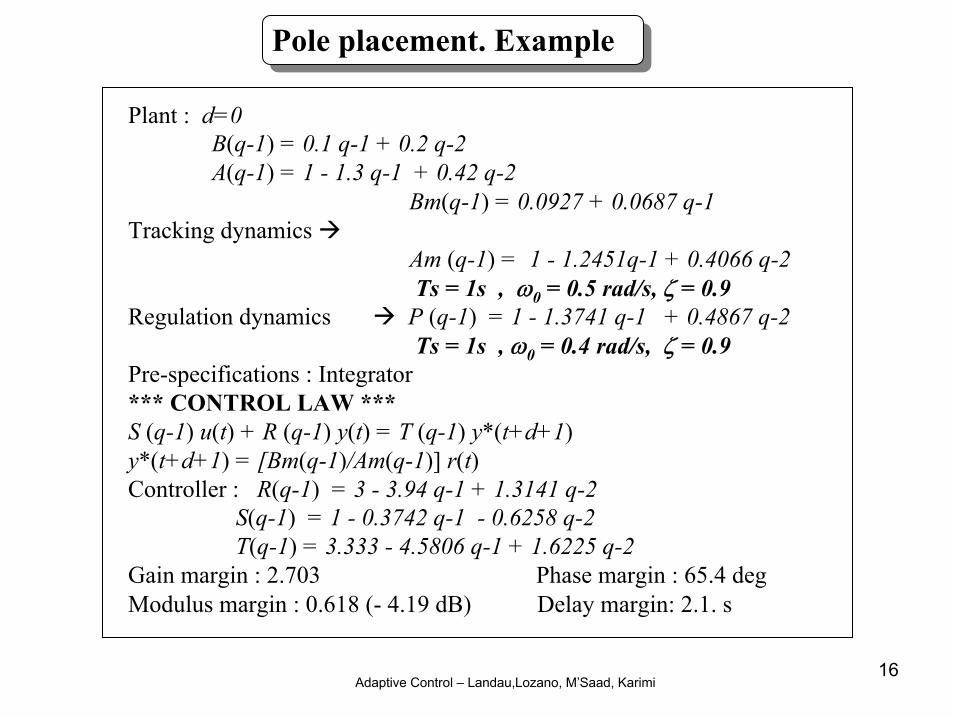
Pole placement. Example
Plant : d=0B(q-1) = 0.1 q-1 + 0.2 q-2A(q-1) = 1 - 1.3 q-1 + 0.42 q-2
Bm(q-1) = 0.0927 + 0.0687 q-1Tracking dynamics
Am (q-1) = 1 - 1.2451q-1 + 0.4066 q-2Ts = 1s , ω0 = 0.5 rad/s, ζ = 0.9
Regulation dynamics P (q-1) = 1 - 1.3741 q-1 + 0.4867 q-2Ts = 1s , ω0 = 0.4 rad/s, ζ = 0.9
Pre-specifications : Integrator*** CONTROL LAW ***S (q-1) u(t) + R (q-1) y(t) = T (q-1) y*(t+d+1)y*(t+d+1) = [Bm(q-1)/Am(q-1)] r(t)Controller : R(q-1) = 3 - 3.94 q-1 + 1.3141 q-2
S(q-1) = 1 - 0.3742 q-1 - 0.6258 q-2T(q-1) = 3.333 - 4.5806 q-1 + 1.6225 q-2
Gain margin : 2.703 Phase margin : 65.4 degModulus margin : 0.618 (- 4.19 dB) Delay margin: 2.1. s
Adaptive Control – Landau,Lozano, M’Saad, Karimi17
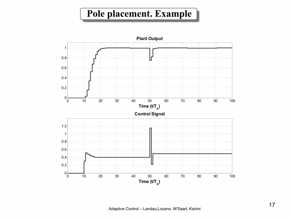
Pole placement. Example
0 10 20 30 40 50 60 70 80 90 1000
0.2
0.4
0.6
0.8
1
Plant Output
Time (t/Ts)
0 10 20 30 40 50 60 70 80 90 1000
0.2
0.4
0.6
0.8
1
1.2
Control Signal
Time (t/Ts)
Adaptive Control – Landau,Lozano, M’Saad, Karimi18
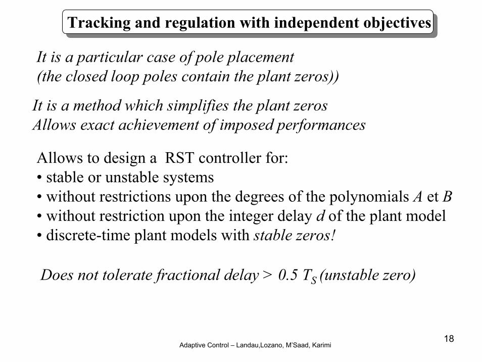
Tracking and regulation with independent objectives
It is a particular case of pole placement(the closed loop poles contain the plant zeros))
Allows to design a RST controller for:• stable or unstable systems• without restrictions upon the degrees of the polynomials A et B• without restriction upon the integer delay d of the plant model• discrete-time plant models with stable zeros!
It is a method which simplifies the plant zerosAllows exact achievement of imposed performances
Does not tolerate fractional delay > 0.5 TS (unstable zero)
Adaptive Control – Landau,Lozano, M’Saad, Karimi19
-1 -0.5 0 0.5 1-1
-0.8
-0.6
-0.4
-0.2
0
0.2
0.4
0.6
0.8
1Zero Admissible Zone
Real Axis
Imag
Axi
sf0/fs = 0.4
0.4
0.3
0.3
0.2
0.2
0.1
0.1
ζ = 0.1 ζ = 0.2
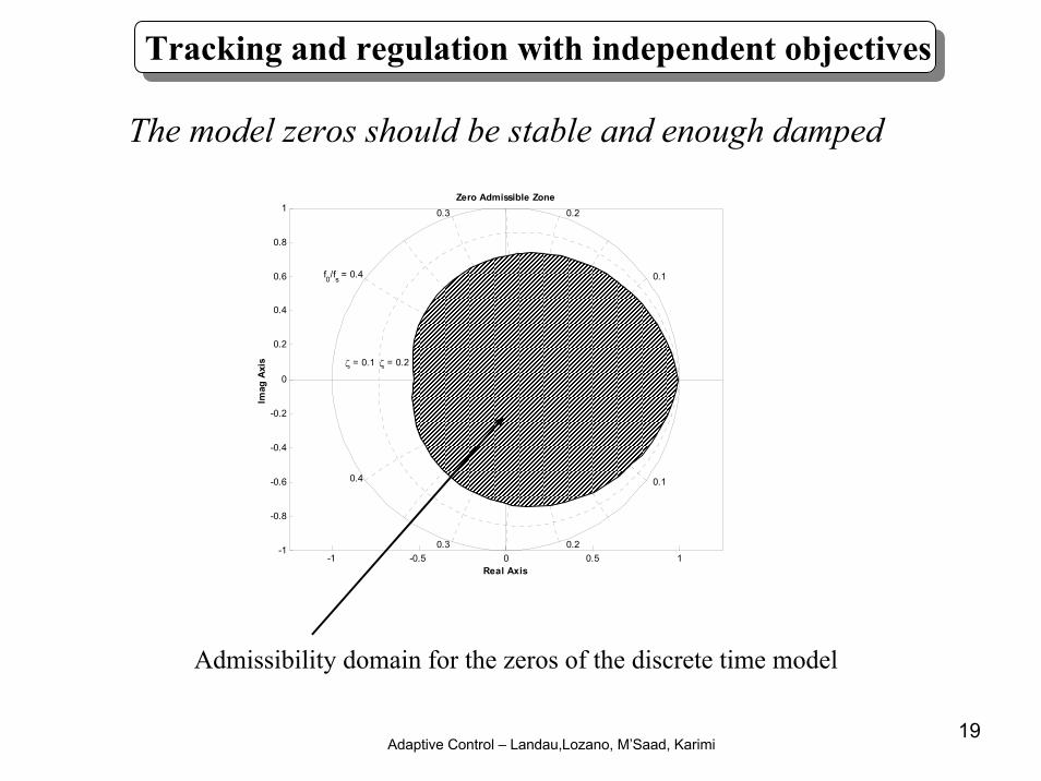
The model zeros should be stable and enough damped
Admissibility domain for the zeros of the discrete time model
Tracking and regulation with independent objectives
Adaptive Control – Landau,Lozano, M’Saad, Karimi20
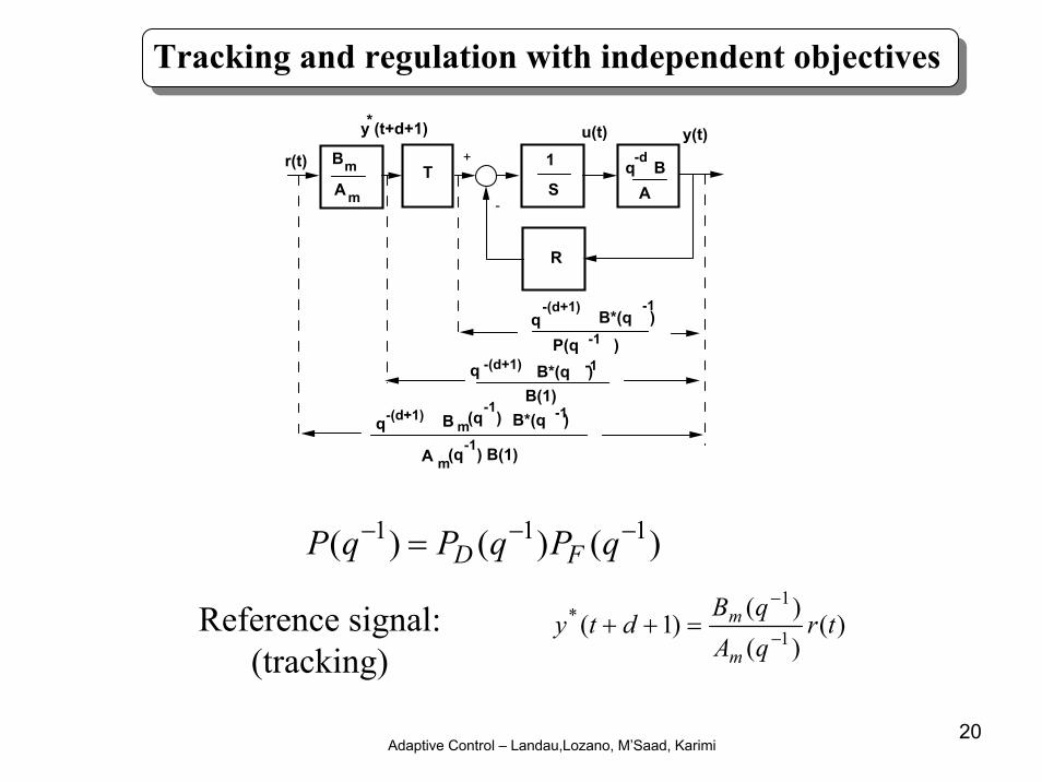
Tracking and regulation with independent objectives
+
-
R
1 q-d
BAS
TA
Bm
m
r(t)
y (t+d+1)*u(t) y(t)
q
-(d+1)
P(q -1 )q
-(d+1)
B*(q )-1
B*(q )
-1
B(1)q
-(d+1) B m(q )
B*(q )
-1-1
A m(q ) B(1)-1
)()()( 111 −−− = qPqPqP FD
)()()(
)1( 1
1* tr
qAqB
dtym
m−
−
=++Reference signal:(tracking)
Adaptive Control – Landau,Lozano, M’Saad, Karimi21
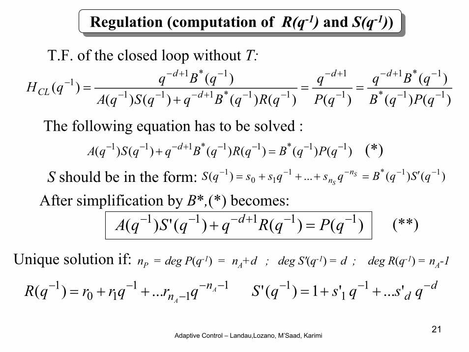
T.F. of the closed loop without T:
)()()(
)()()()()()()( 11*
1*1
1
1
11*111
1*11
−−
−+−
−
+−
−−+−−−
−+−− ==
+=
qPqBqBq
qPq
qRqBqqSqAqBqqH
dd
d
d
CL
)()()()()()( 11*11*111 −−−−+−−− =+ qPqBqRqBqqSqA d
The following equation has to be solved :
S should be in the form: )()(...)( 11*110
1 −−−−− ′=+++= qSqBqsqssqS SS
nn
After simplification by B*,(*) becomes:)()()(')( 11111 −−+−−− =+ qPqRqqSqA d
(*)
nP = deg P(q-1) = nA+d ; deg S'(q-1) = d ; deg R(q-1) = nA-1Unique solution if:1
11
101 ...)( −−
−−− ++= A
A
nn qrqrrqR d
d qsqsqS −−− ++= '...'1)(' 11
1
(**)
Regulation (computation of R(q-1) and S(q-1))
Adaptive Control – Landau,Lozano, M’Saad, Karimi22
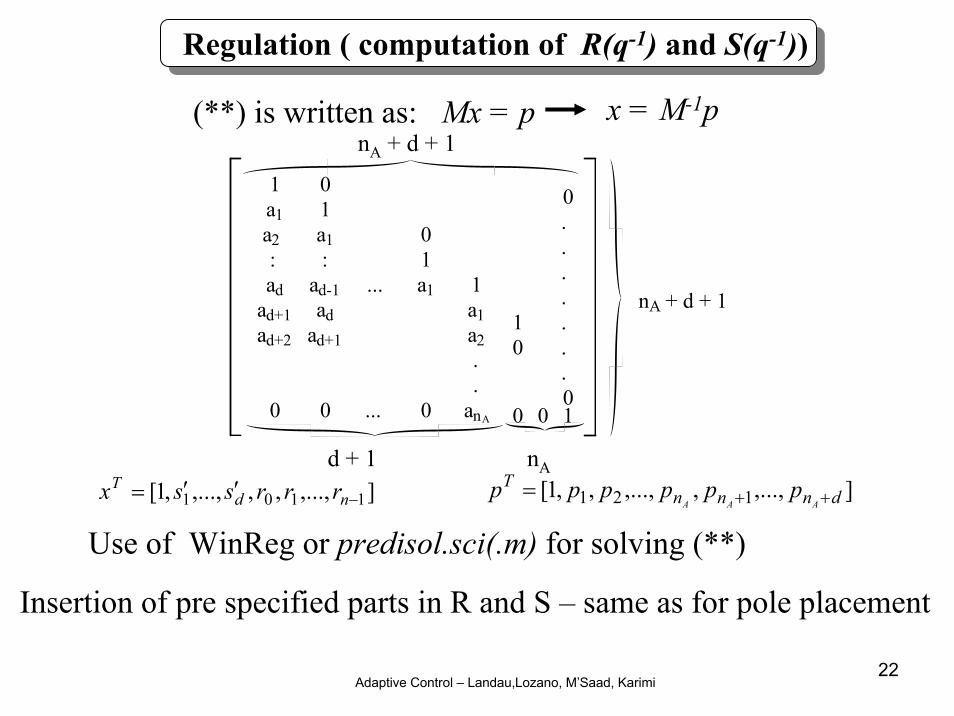
(**) is written as: Mx = p
1 0 a1 1 a2 a1 0: : 1ad ad-1 ... a1 1
ad+1 ad a1ad+2 ad+1 a2
. .0 0 ... 0 anA
0 . .
. .
1 . 0 .
. 00 0 1
nA + d + 1
nA + d + 1
d + 1 nA],...,,,,...,,1[ 1101 −′′= nd
T rrrssx ],...,,,...,,,1[ 121 dnnnT
AAApppppp ++=
Use of WinReg or predisol.sci(.m) for solving (**)
x = M-1p
Insertion of pre specified parts in R and S – same as for pole placement
Regulation ( computation of R(q-1) and S(q-1))
Adaptive Control – Landau,Lozano, M’Saad, Karimi23
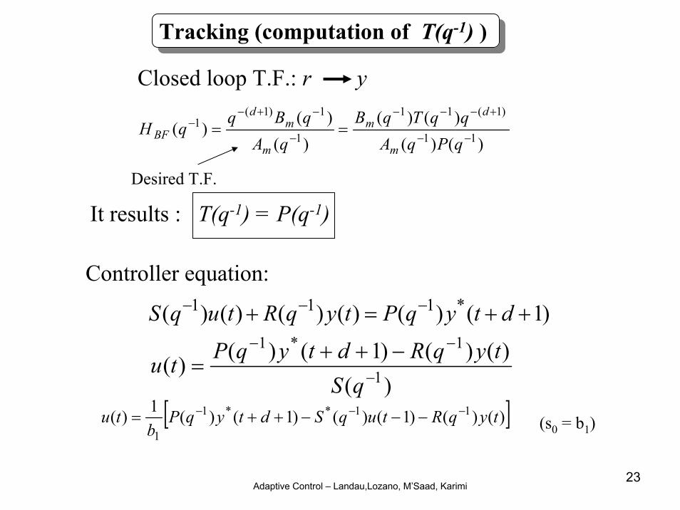
Tracking (computation of T(q-1) )
Closed loop T.F.: r y
)()()()(
)()(
)( 11
)1(11
1
1)1(1
−−
+−−−
−
−+−− ==
qPqAqqTqB
qAqBq
qHm
dm
m
md
BF
Desired T.F.
It results : T(q-1) = P(q-1)
Controller equation:
)1()()()()()( *111 ++=+ −−− dtyqPtyqRtuqS
)()()()1()()( 1
1*1
−
−− −++=
qStyqRdtyqPtu
[ ])()()1()()1()(1)( 11**1
1tyqRtuqSdtyqP
btu −−− −−−++= (s0 = b1)
Adaptive Control – Landau,Lozano, M’Saad, Karimi24
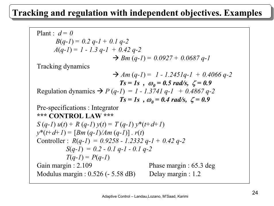
Tracking and regulation with independent objectives. Examples
Plant : d = 0B(q-1) = 0.2 q-1 + 0.1 q-2
A(q-1) = 1 - 1.3 q-1 + 0.42 q-2Bm (q-1) = 0.0927 + 0.0687 q-1
Tracking dynamics Am (q-1) = 1 - 1.2451q-1 + 0.4066 q-2Ts = 1s , ω0 = 0.5 rad/s, ζ = 0.9
Regulation dynamics P (q-1) = 1 - 1.3741 q-1 + 0.4867 q-2Ts = 1s , ω0 = 0.4 rad/s, ζ = 0.9
Pre-specifications : Integrator*** CONTROL LAW ***S (q-1) u(t) + R (q-1) y(t) = T (q-1) y*(t+d+1)y*(t+d+1) = [Bm (q-1)/Am (q-1)] . r(t)Controller : R(q-1) = 0.9258 - 1.2332 q-1 + 0.42 q-2
S(q-1) = 0.2 - 0.1 q-1 - 0.1 q-2T(q-1) = P(q-1)
Gain margin : 2.109 Phase margin : 65.3 degModulus margin : 0.526 (- 5.58 dB) Delay margin : 1.2
Adaptive Control – Landau,Lozano, M’Saad, Karimi25
0 10 20 30 40 50 60 70 80 90 1000
0.2
0.4
0.6
0.8
1
Plant Output
Time (t/Ts)
0 10 20 30 40 50 60 70 80 90 100-0.5
0
0.5
1
1.5
Control Signal
Time (t/Ts)
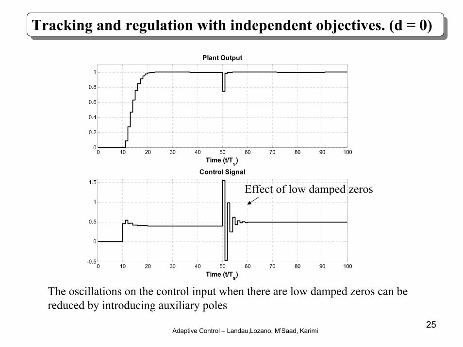
Tracking and regulation with independent objectives. (d = 0)
Effect of low damped zeros
The oscillations on the control input when there are low damped zeros can bereduced by introducing auxiliary poles
Adaptive Control – Landau,Lozano, M’Saad, Karimi26
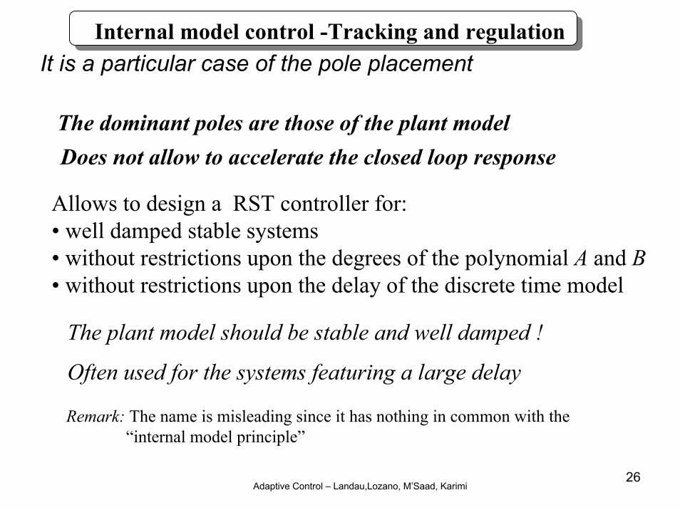
Internal model control -Tracking and regulationIt is a particular case of the pole placement
The dominant poles are those of the plant model
Allows to design a RST controller for:• well damped stable systems• without restrictions upon the degrees of the polynomial A and B• without restrictions upon the delay of the discrete time model
The plant model should be stable and well damped !
Does not allow to accelerate the closed loop response
Often used for the systems featuring a large delay
Remark: The name is misleading since it has nothing in common with the“internal model principle”
Adaptive Control – Landau,Lozano, M’Saad, Karimi27
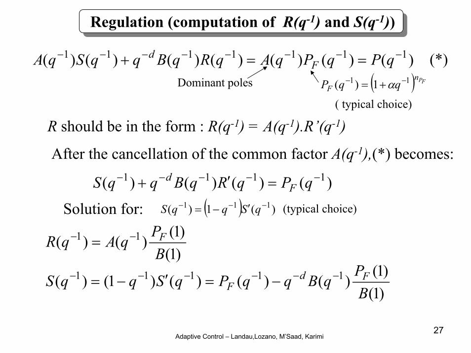
)()()()()()()( 1111111 −−−−−−−− ==+ qPqPqAqRqBqqSqA Fd
Dominant poles ( ) FPnF qqP 11 1)( −− += α
( typical choice)
(*)
R should be in the form : R(q-1) = A(q-1).R’(q-1)
)()()()( 1111 −−−−− =′+ qPqRqBqqS Fd
After the cancellation of the common factor A(q-1),(*) becomes:
( ) )(1)( 111 −−− ′−= qSqqS (typical choice) Solution for:
)1()1()()( 11
BPqAqR F−− =
)1()1()()()()1()( 11111
BPqBqqPqSqqS Fd
F−−−−−− −=′−=
Regulation (computation of R(q-1) and S(q-1))
Adaptive Control – Landau,Lozano, M’Saad, Karimi28
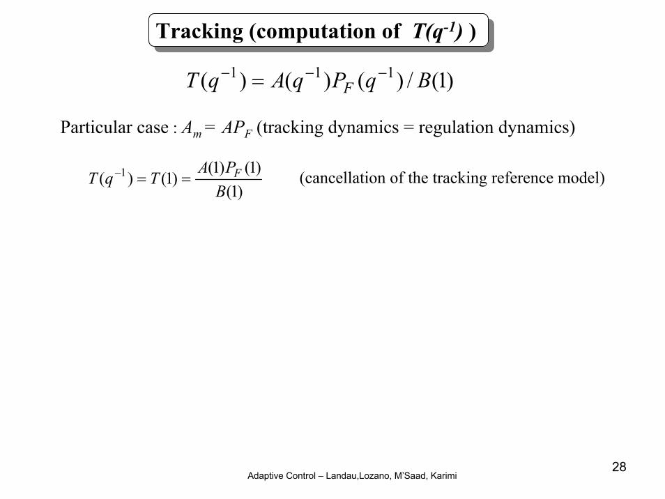
)1(/)()()( 111 BqPqAqT F−−− =
Particular case : Am = APF (tracking dynamics = regulation dynamics)
)1()1()1(
)1()( 1
BPA
TqT F==− (cancellation of the tracking reference model)
Tracking (computation of T(q-1) )
Adaptive Control – Landau,Lozano, M’Saad, Karimi29
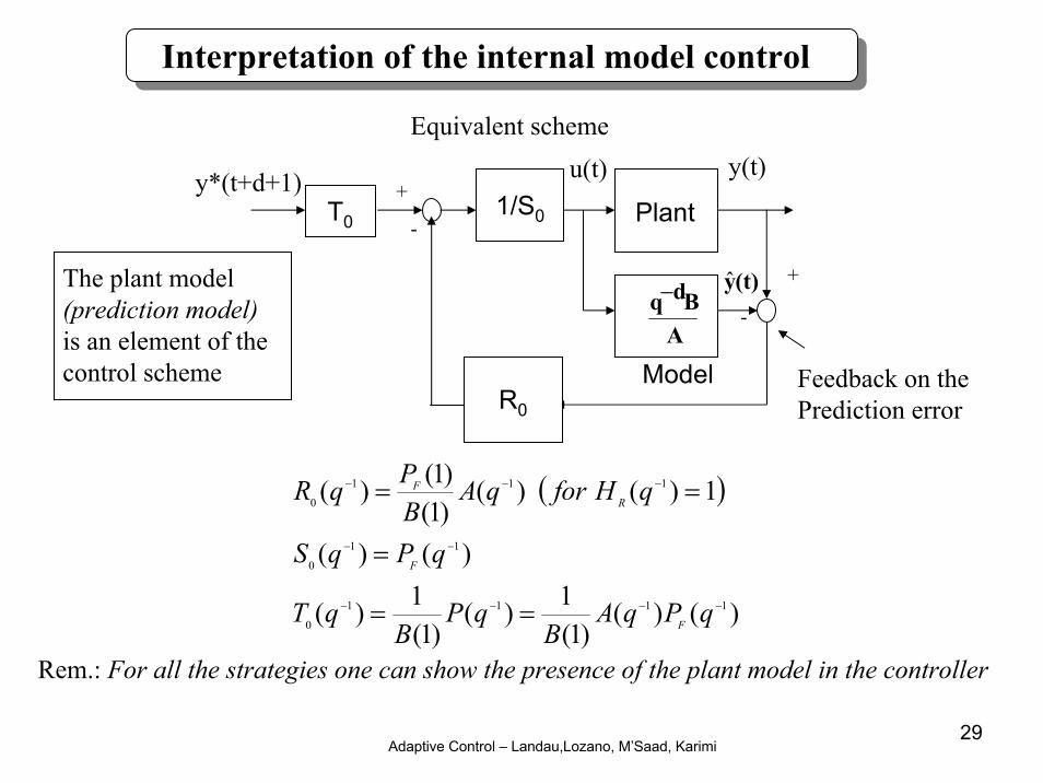
Interpretation of the internal model control
Equivalent scheme
( )
)()()1(
1)()1(
1)(
)()(
1)()()1()1()(
1111
0
11
0
111
0
−−−−
−−
−−−
==
=
==
qPqAB
qPB
qT
qPqS
qHforqABPqR
F
F
RF
T0
+
+
-
-1/S0 Plant
ABdq−
Model
y*(t+d+1) u(t)
(t)y
y(t)
R0
The plant model(prediction model)is an element of thecontrol scheme Feedback on the
Prediction error
Rem.: For all the strategies one can show the presence of the plant model in the controller
Adaptive Control – Landau,Lozano, M’Saad, Karimi30
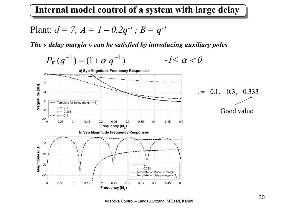
Internal model control of a system with large delay
Plant: d = 7; A = 1 – 0.2q-1 ; B = q-1
The « delay margin » can be satisfied by introducing auxiliary poles
) 1()( 11 −− += qqPF α -1< α < 0
α = −0.1; −0.3; −0.333
Good value
0 0.05 0.1 0.15 0.2 0.25 0.3 0.35 0.4 0.45 0.5
-30
-20
-10
0
b) Syp Magnitude Frequency Responses
Frequency (f/fs)
Mag
nitu
de (d
B)
0 0.05 0.1 0.15 0.2 0.25 0.3 0.35 0.4 0.45 0.5-10
-8
-6
-4
-2
0a) Syb Magnitude Frequency Responses
Frequency (f/fs)
Mag
nitu
de (d
B)
α = -0.1α = -0.333Template for Modulus marginTemplate for Delay margin = Ts
Template for Delay margin = Tsα = -0.1α = -0.333α = -0.3

Adaptive Control – Landau,Lozano, M’Saad, Karimi31
11 1)( −− += qqH R corresponds to the opening of the loop at 0.5fS
Internal model control of a system with large delay
See also:I.D. Landau (1995) : Robust digital control of systems with time delay (the Smith predictor revisited)Int. J. of Control, v.62,no.2 pp 325-347
0 0.05 0.1 0.15 0.2 0.25 0.3 0.35 0.4 0.45 0.5-30
-20
-10
0
b) Syp Magnitude Frequency Responses
Frequency (f/fs)
Mag
nitu
de (d
B)
0 0.05 0.1 0.15 0.2 0.25 0.3 0.35 0.4 0.45 0.5-10
-8
-6
-4
-2
0a) Syb Magnitude Frequency Responses
Frequency (f/fs)
Mag
nitu
de (d
B)
HR = 1, PF = 1 - 0.333q-1
HR = 1 + q-1, PF = 1
Template for Modulus marginTemplate for Delay margin = Ts
Template for Delay margin = TsHR = 1, PF = 1 - 0.333q-1
HR = 1 + q-1, PF = 1
Adaptive Control – Landau,Lozano, M’Saad, Karimi32
Minimum Variance Tracking and Regulation
Adaptive Control – Landau,Lozano, M’Saad, Karimi33
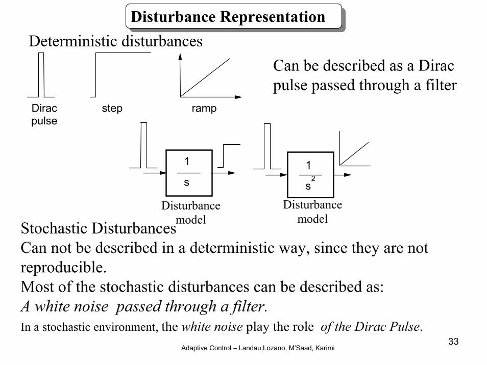
Disturbance RepresentationDeterministic disturbances
Stochastic DisturbancesCan not be described in a deterministic way, since they are not reproducible.Most of the stochastic disturbances can be described as:A white noise passed through a filter.In a stochastic environment, the white noise play the role of the Dirac Pulse.
Can be described as a Diracpulse passed through a filter
rampstep Dirac pulse
Disturbance model
1
s1
s2
Disturbance model
Adaptive Control – Landau,Lozano, M’Saad, Karimi34
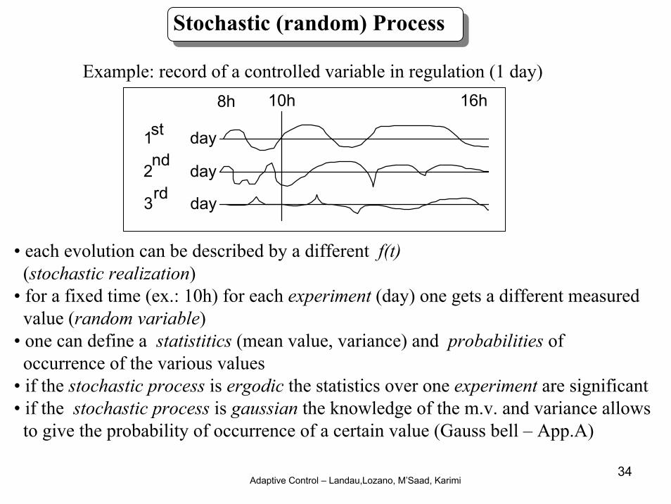
Stochastic (random) Process
Example: record of a controlled variable in regulation (1 day)
• each evolution can be described by a different f(t)(stochastic realization)
• for a fixed time (ex.: 10h) for each experiment (day) one gets a different measuredvalue (random variable)
• one can define a statistitics (mean value, variance) and probabilities of occurrence of the various values
• if the stochastic process is ergodic the statistics over one experiment are significant• if the stochastic process is gaussian the knowledge of the m.v. and variance allowsto give the probability of occurrence of a certain value (Gauss bell – App.A)
16h10h8h
1 day st
2 day nd
3 day rd
Adaptive Control – Landau,Lozano, M’Saad, Karimi35
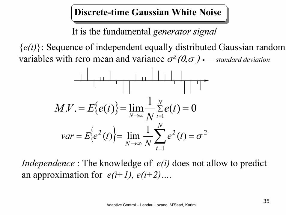
Discrete-time Gaussian White Noise
It is the fundamental generator signal{e(t)}: Sequence of independent equally distributed Gaussian randomvariables with rero mean and variance σ2 (0,σ ) standard deviation
{ } 0)(1lim)(..1
=== ∑=∞→
N
tNte
NteEVM
{ } 2
1
22 )(1lim)( σ=== ∑=
∞→
N
tN
teN
teEvar
Independence : The knowledge of e(i) does not allow to predictan approximation for e(i+1), e(i+2)….
Adaptive Control – Landau,Lozano, M’Saad, Karimi36
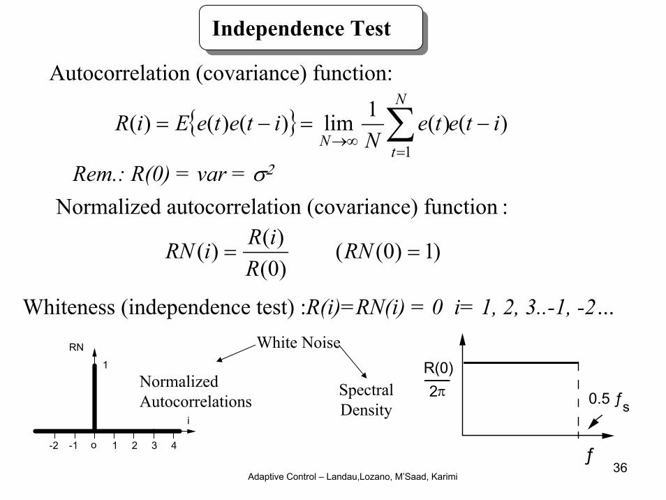
Independence Test
Autocorrelation (covariance) function:
{ } )()(1lim)()()(1
iteteN
iteteEiRN
tN
−=−= ∑=
∞→
Rem.: R(0) = var = σ2
Normalized autocorrelation (covariance) function :
)1)0(()0()()( == RN
RiRiRN
Whiteness (independence test) :R(i)=RN(i) = 0 i= 1, 2, 3..-1, -2…White Noise
SpectralDensity
1
RN
i
o 1 2 3 4-1-2
NormalizedAutocorrelations
0.5 ƒ s
ƒ
- - - - - - - - - R(0)2 π

Adaptive Control – Landau,Lozano, M’Saad, Karimi37
Moving Average Process – MA
e(t)1+ c
1q -1
y(t) )()1()1()()( 111 teqctectety −+=−+=
{ } ∑∑∑===
=−+===N
t
N
t
N
t
teN
cteN
tyN
tyEMV1
111
0)1(1)(1)(1)(..
{ } 221
1
22 )1()(1)()0( σctyN
tyERN
ty +=∑==
=
{ } 221
1
21
1
)(1)1()(1)1()()1( σctecN
tytyN
tytyERN
t
N
ty ==−=−= ∑∑
==
0..)3()2( === yy RR
0 +1 2-1-2
-----------c1
1+c12
(c >0)1RN1
i
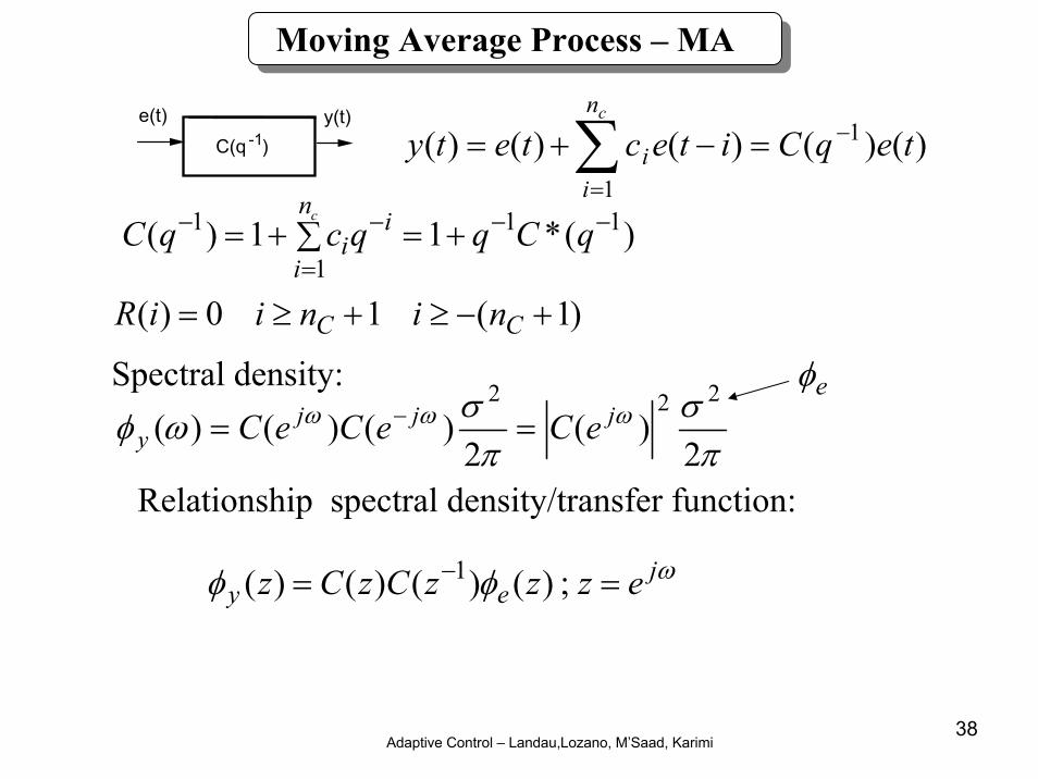
Adaptive Control – Landau,Lozano, M’Saad, Karimi38
e(t) y(t)-1C(q ) )()()()()( 1
1
teqCitectetycn
ii
−
=
=−+= ∑)(*11)( 11
1
1 −−
=
−− +=∑+= qCqqcqCcn
i
ii
)1(10)( +−≥+≥= CC niniiR
πσ
πσωφ ωωω
2)(
2)()()(
222jjj
y eCeCeC == −
Spectral density:
ωφφ jey ezzzCzCz == − ;)()()()( 1
Relationship spectral density/transfer function:
eφ
Moving Average Process – MA
Adaptive Control – Landau,Lozano, M’Saad, Karimi39
------------------1
1+ a1 q- 1
y(t)e(t)
-------------1
A( q-1)
y(t)e(t)
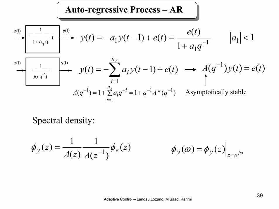
Auto-regressive Process – AR
11
)()()1()( 111
1 <+
=+−−=−
aqa
tetetyaty
)()1()(1
tetyatyAn
ii +−−= ∑
=
)(*11)( 11
1
1 −−
=
−− +=∑+= qAqqaqAAn
i
ii
)()()( 1 tetyqA =−
Asymptotically stable
Spectral density:
)()(
1)(
1)( 1 zzAzA
z ey φφ−
=ωφωφ jezyy z
== )()(
Adaptive Control – Landau,Lozano, M’Saad, Karimi40
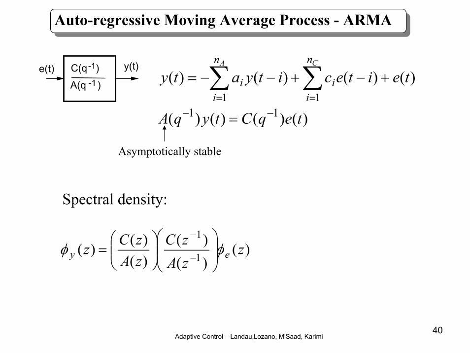
Auto-regressive Moving Average Process - ARMA
C(q )-1
A(q )-1
y(t)e(t) )()()()(11
teitecityatyCA n
ii
n
ii +−+−−= ∑∑
==
)()()()( 11 teqCtyqA −− =
Asymptotically stable
)()()(
)()()( 1
1z
zAzC
zAzCz ey φφ ⎟
⎟⎠
⎞⎜⎜⎝
⎛⎟⎟⎠
⎞⎜⎜⎝
⎛=
−
−
Spectral density:
Adaptive Control – Landau,Lozano, M’Saad, Karimi41
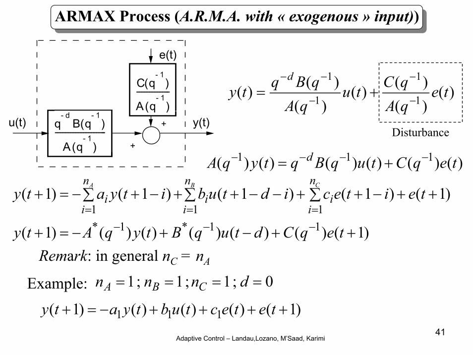
ARMAX Process (A.R.M.A. with « exogenous » input))
--------------------q
- d B(q
- 1)
A(q- 1
)
y(t)
-------------C(q
- 1)
A(q- 1
)+
+
u(t)
e(t)
)()()()(
)()()( 1
1
1
1te
qAqCtu
qAqBqty
d
−
−
−
−−
+=
Disturbance
)()()()()()( 111 teqCtuqBqtyqA d −−−− +=
)1()()()()()()1(
)1()1()1()1()1(
11*1*1 11
++−+−=+
++∑ ∑ −++−−+∑ +−+−=+
−−−= ==
teqCdtuqBtyqAty
teitecidtubityatyB CA n
i
n
iii
n
ii
Example: 0;1;1;1 ==== dnnn CBA
)1()()()()1( 111 ++++−=+ tetectubtyaty
Remark: in general nC = nA
Adaptive Control – Landau,Lozano, M’Saad, Karimi42
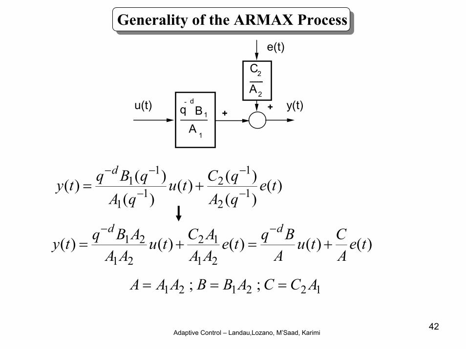
Generality of the ARMAX Process
q- d
B1
A1
------C2
A2
y(t)
e(t)
u(t) ++
)()()()(
)()()( 1
2
12
11
11 te
qAqCtu
qAqBqty
d
−
−
−
−−+=
)()()()()(21
12
21
21 teACtu
ABqte
AAACtu
AAABqty
dd+=+=
−−
122121 ;; ACCABBAAA ===
Adaptive Control – Landau,Lozano, M’Saad, Karimi43
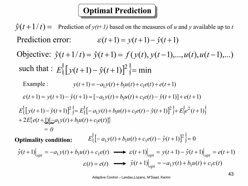
Optimal Prediction
=+ )/1(ˆ tty Prediction of y(t+1) based on the measures of u and y available up to t
Prediction error: )1(ˆ)1()1( +−+=+ tytytε
Objective: ),...)1(),(),...,1(),(()1(ˆ)/1(ˆ −−=+=+ tututytyftytty
such that : [ ]{ } min)1(ˆ)1( 2 =+−+ tytyE)1()()()()1( 111 ++++−=+ tetectubtyaty
)1()]1(ˆ)()()([)1(ˆ)1()1( 111 +++−++−=+−+=+ tetytectubtyatytytε
[ ]{ } [ ]{ } { }{ })]()()()[1(2
)1()1(ˆ)()()( )1(ˆ)1(
111
22111
2
tectubtyateEteEtytectubtyaEtytyE
++−+++++−++−=+−+
= 0
{
[ ]{ } 0)1(ˆ)()()( 2111 =+−++− tytectubtyaEOptimality condition:
)()()()1(ˆ 111 tectubtyaty opt ++−=+ )1()1(ˆ)1()1( +=+−+=+ tetytyt optoptε
Example :
)()( tet =ε )()()()1(ˆ 111 tctubtyaty opt ε++−=+

Adaptive Control – Landau,Lozano, M’Saad, Karimi44
Optimal prediction
)1()()()()()()1( 11*1* ++−+−=+ −−− teqCdtuqBtyqAty
)()()()()()()1(ˆ 1*1*1* teqCdtuqBtyqAty −−− +−+−=+
)1()1(ˆ)1()1( +=+−+=+ tetytyt optε
)()()()()()()1(ˆ 1*1*1* tqCdtuqBtyqAty ε−−− +−+−=+
ARMAX:
Optimal predictor (theoretical):
Prediction error:
Optimal predictor (implementation):
One replaces the unknown white noise by the prediction error
Adaptive Control – Landau,Lozano, M’Saad, Karimi45
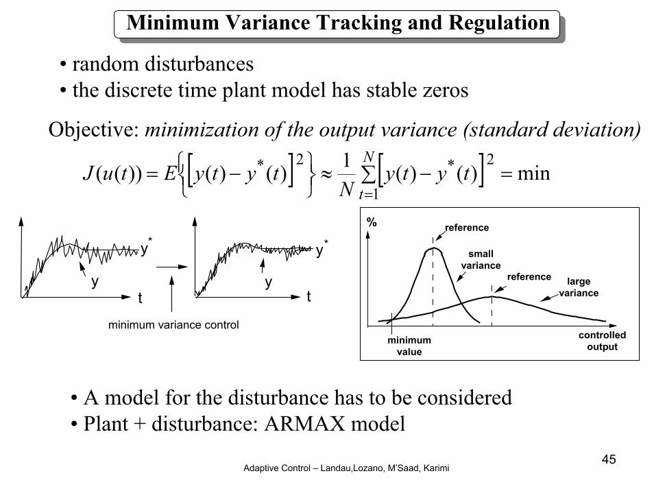
Minimum Variance Tracking and Regulation
• random disturbances• the discrete time plant model has stable zeros
Objective: minimization of the output variance (standard deviation)
[ ] [ ] min)()(1)()())((1
2 *2 * =∑ −≈⎭⎬⎫
⎩⎨⎧ −=
=
N
ttyty
NtytyEtuJ
• A model for the disturbance has to be considered• Plant + disturbance: ARMAX model
minimum variance control
y
y
**
t t
y
y
%
minimumvalue
controlled output
largevariance
reference
reference
smallvariance
Adaptive Control – Landau,Lozano, M’Saad, Karimi46
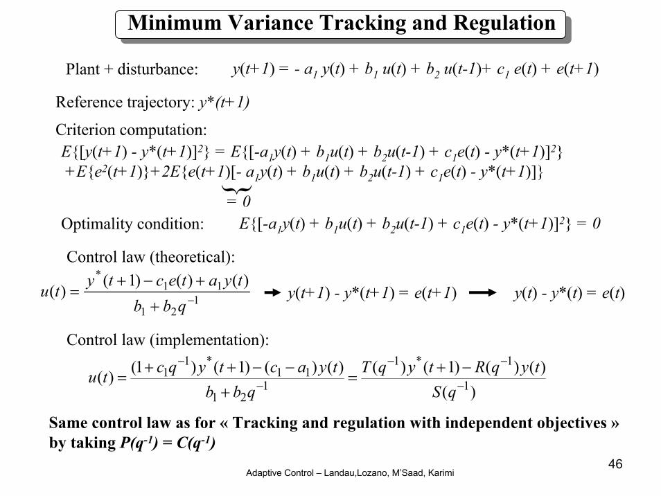
y(t+1) = - a1 y(t) + b1 u(t) + b2 u(t-1)+ c1 e(t) + e(t+1)Plant + disturbance:
Reference trajectory: y*(t+1)
Criterion computation:E{[y(t+1) - y*(t+1)]2} = E{[-a1y(t) + b1u(t) + b2u(t-1) + c1e(t) - y*(t+1)]2}+E{e2(t+1)}+2E{e(t+1)[- a1y(t) + b1u(t) + b2u(t-1) + c1e(t) - y*(t+1)]}
{= 0Optimality condition: E{[-a1y(t) + b1u(t) + b2u(t-1) + c1e(t) - y*(t+1)]2} = 0
Control law (theoretical):
121
11* )()()1()(
−+
+−+=
qbbtyatectytu y(t+1) - y*(t+1) = e(t+1) y(t) - y*(t) = e(t)
)()()()1()()()()1()1()( 1
1*1
121
11*1
1−
−−
−
− −+=
+−−++
=qS
tyqRtyqTqbb
tyactyqctu
Control law (implementation):
Same control law as for « Tracking and regulation with independent objectives »by taking P(q-1) = C(q-1)
Minimum Variance Tracking and Regulation
Adaptive Control – Landau,Lozano, M’Saad, Karimi47
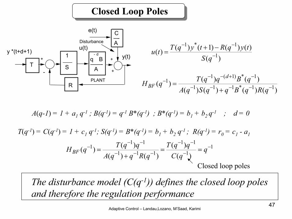
Closed Loop Poles
Disturbance
T
y *(t+d+1)1
R
+
-PLANT
u(t)
S ---------q
- dB
A
y(t)
-----C
A
+
+
e(t)
)()()()1()()( 1
1*1
−
−− −+=
qStyqRtyqTtu
)()()()()()()( 11*111
1*)1(11
−−−−−
−+−−−
+=
qRqBqqSqAqBqqTqH
d
BF
A(q-1) = 1 + a1 q-1 ; B(q-1) = q-1 B*(q-1) ; B*(q-1) = b1 + b2 q-1 ; d = 0
T(q-1) = C(q-1) = 1 + c1 q-1; S(q-1) = B*(q-1) = b1 + b2 q-1 ; R(q-1) = r0 = c1 - a1
11
11
111
111
)()(
)()()()( −
−
−−
−−−
−−− ==
+= q
qCqqT
qRqqAqqTqHBF
Closed loop poles
The disturbance model (C(q-1)) defines the closed loop polesand therefore the regulation performance

Adaptive Control – Landau,Lozano, M’Saad, Karimi48
Minimum Variance Tracking and Regulation – general case
Same computations as for « tracking and regulation with independentobjectives » by taking P(q-1) = C(q-1) (see Chapter 3)
r(t)
DISTURBANCE
------Bm
AmT
y *(t+d+1)1
R
+
-PLANT
- - - - - - - - - - -----------q -(d+1)
C(q-1)
q- (d+1)
----------------------------q
- (d+1)
u(t)
S ---------q
- dB
A
y(t)
-----CA
+
+
e(t)
Am(q-1)
Bm(q-1)
Adaptive Control – Landau,Lozano, M’Saad, Karimi49
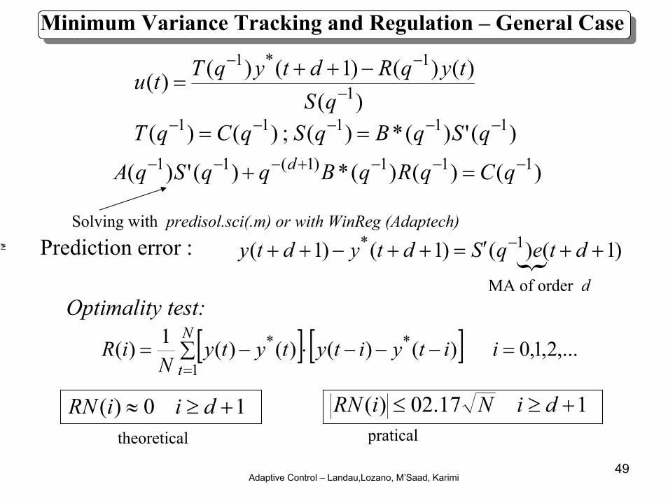
)()()()1()()( 1
1*1
−
−− −++=
qStyqRdtyqTtu
)(')(*)(;)()( 11111 −−−−− == qSqBqSqCqT
)()()(*)(')( 111)1(11 −−−+−−− =+ qCqRqBqqSqA d
Solving with predisol.sci(.m) or with WinReg (Adaptech)
)1()()1()1( 1* ++′=++−++ − dteqSdtydtyPrediction error : MA of order d
{
[ ] [ ]∑ =−−−⋅−==
N
tiityitytyty
NiR
1
** ,...2,1,0)()()()(1)(
≈≥
10)( +≥≈ diiRN 117.02)( +≥≤ diNiRN
Optimality test:
theoretical pratical
Minimum Variance Tracking and Regulation – General Case

Adaptive Control – Landau,Lozano, M’Saad, Karimi50
Plant: • d = 0• B(q-1) = 0.2 q-1 + 0.1 q-2• A(q-1) = 1 - 1.3 q-1 + 0.42 q-2 Tracking dynamics Ts = 1s, ω0 = 0.5 rad/s, ζ = 0.9• Bm = +0.0927 +0.0687 q-1 • Am = 1 - 1.2451 q-1 + 0.4066 q-2Disturbance polynomial C(q-1) = 1 -1.34 q-1 + 0.49 q-2Pre-specifications: Integrator*** CONTROL LAW *** S(q-1) u(t) + R(q-1) y(t) = T(q-1) y*(t+d+1)y*(t+d+1) = [(Bmq-1)/Am(q-1)] . ref(t)Controller: • R(q-1) = 0.96 - 1.23 q-1 + 0.42 q-2• S(q-1) = 0.2 - 0.1 q-1 - 0.1 q-2• T(q-1) = C(q-1)Gain margin: 2.084 Phase margin: 61.8 degModulus margin: 0.520 (- 5.68 dB) Delay margin: 1.3 s
Minimum Variance Tracking and Regulation. Example

Adaptive Control – Landau,Lozano, M’Saad, Karimi51
Poursuite et régulation à variance minimale.Exemple
Attention: For robustness and actuator stress one may be obligedto add auxiliary poles (see book pg. 190)
50 100 150 200 250 300 350 400
-0.2
0
0.2
0.4
0.6
0.8
1
Process Output
Controller OFF Controller ON
Am
plitu
de MeasureReference
50 100 150 200 250 300 350 400-1
-0.5
0
0.5
1
Control Signal
Am
plitu
de
Time (t/Ts)
Minimum Variance Tracking and Regulation. Example
Adaptive Control – Landau,Lozano, M’Saad, Karimi52
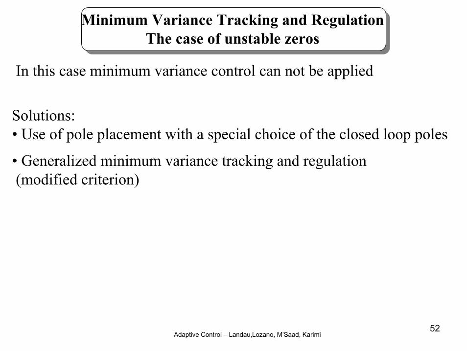
Minimum Variance Tracking and RegulationThe case of unstable zeros
In this case minimum variance control can not be applied
Solutions:• Use of pole placement with a special choice of the closed loop poles
• Generalized minimum variance tracking and regulation(modified criterion)
Adaptive Control – Landau,Lozano, M’Saad, Karimi53
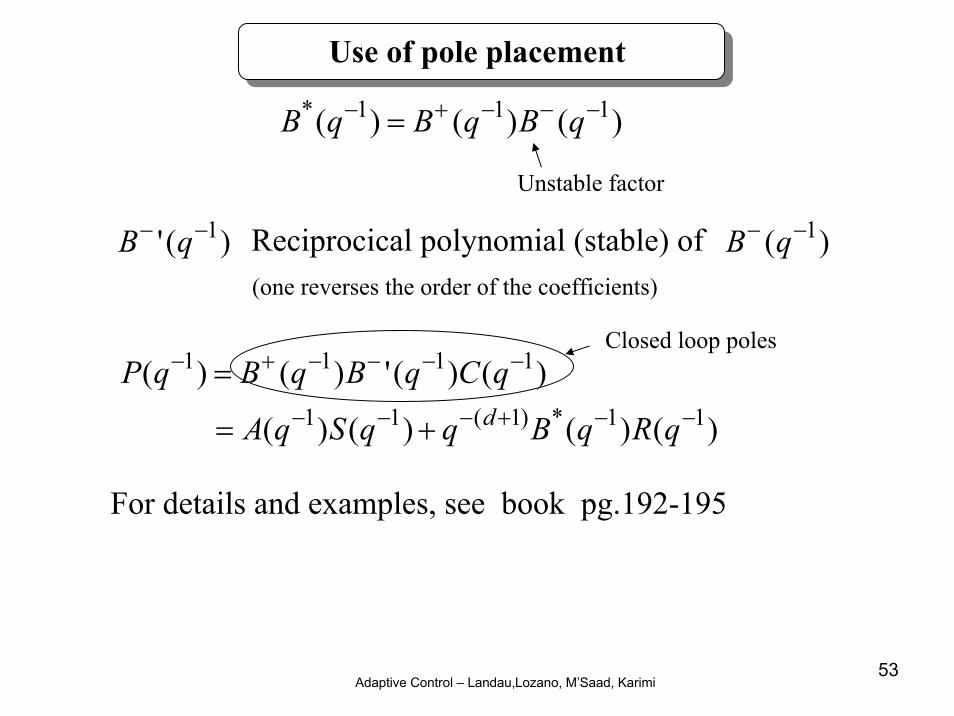
)()()( 111* −−−+− = qBqBqB
)(' 1−− qB Reciprocical polynomial (stable) of )( 1−− qB
)()()()(
)()(')()(11*)1(11
1111
−−+−−−
−−−−+−
+=
=
qRqBqqSqA
qCqBqBqPd
Use of pole placement
Unstable factor
Closed loop poles
For details and examples, see book pg.192-195
(one reverses the order of the coefficients)

Adaptive Control – Landau,Lozano, M’Saad, Karimi54
Generalized Minimum Variance Tracking and Regulation
Criterion:
min)()()()1()1(
2
1
1* =
⎪⎭
⎪⎬⎫
⎪⎩
⎪⎨⎧
⎥⎦
⎤⎢⎣
⎡+++−++ −
−tu
qCqQdtydtyE
1
11
1)1()( −
−−
+−
=qqqQ
αλ
Particular case : α = 0
min)1()]1()([)(
)1(2
*1
=⎪⎭
⎪⎬⎫
⎪⎩
⎪⎨⎧
⎥⎦
⎤⎢⎣
⎡++−−−+++
−dtytutu
qCdtyE λ
Controllere:)()(
)()()1()()( 11
1*1
−−
−−
+−++
=qQqS
tyqRdtyqCtu
Allows to stabilize the controller and the system(but not always!)
Weighting the control variations
Adaptive Control – Landau,Lozano, M’Saad, Karimi55
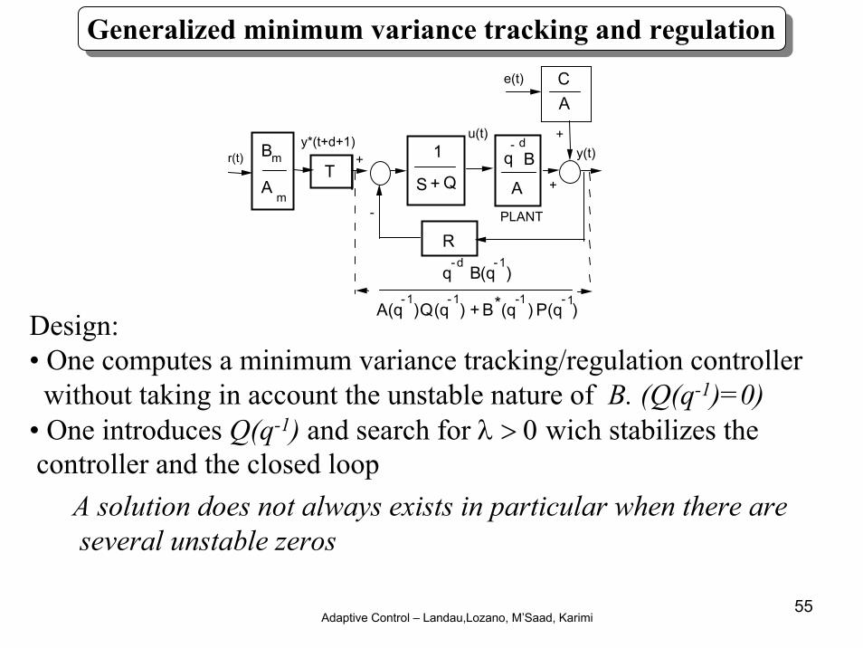
Generalized minimum variance tracking and regulation
Design:• One computes a minimum variance tracking/regulation controllerwithout taking in account the unstable nature of B. (Q(q-1)=0)
• One introduces Q(q-1) and search for λ > 0 wich stabilizes the controller and the closed loop
A solution does not always exists in particular when there areseveral unstable zeros
Q
u(t)
R
T+
-
y*(t+d+1)
q- d
B(q-1
)
A(q- 1
)Q(q- 1
) + B*(q-1
) P(q- 1)
r(t) Bm
Am
1
S +
y(t)
PLANT
q- d
B
A
CA
e(t)
+
+
Copyright © 2022 FDOKUMEN