Adaptive Control of a MEMS Steering Mirror for Suppression ofLaser Beam Jitter

Nestor O. Perez Arancibia, Neil Chen, Steve Gibson, and Tsu-Chin Tsao

Abstract— This paper presents an adaptive control schemefor laser-beam steering by a two-axis MEMS tilt mirror.Disturbances in the laser beam are rejected by a µ-synthesisfeedback controller augmented by the adaptive control loop,which determines control gains that are optimal for thecurrent disturbance acting on the laser beam. The adaptiveloop is based on an adaptive lattice filter that implicitlyidentifies the disturbance statistics from real-time sensordata. Experimental results are presented to demonstrate thatthe adaptive controller significantly extends the disturbance-rejection bandwidth achieved by the feedback controller alone.

I. INTRODUCTION

Laser beam steering has a wide range of applicationsin fields such as adaptive optics, wireless communications,and manufacturing process. The control problem is toposition the centroid of a laser beam at a desired locationon a target plane some distance from the laser sourcewith minimal beam motion, or jitter, in the presence ofdisturbances. In applications, the jitter usually is producedby vibration of the optical bench or turbulence in theatmosphere through which the beam travels. Turbulence-induced jitter may be rather broadband [1], [2], [3], [4],while vibration-induced jitter typically is composed of oneor more narrow bandwidths produced by vibration modesof the structure supporting the optical system. Because thedisturbance characteristics often change with time, optimalperformance of a beam steering system requires an adaptivecontrol system.

In engineering applications, lightly damped elastic modesof the beam steering mirrors also produce beam jitter. Thisis the case with the MEMS mirrors used in the experimentpresented here. These mirrors, which are used in free-spaceoptical communications systems, have a torsional vibrationmode about each steering axis.

This paper presents a control scheme for laser beamsteering in which a linear-time-invariant (LTI) feedbackcontrol loop is augmented by an adaptive control loop. TheLTI feedback loop used here is a µ-synthesis controllerdesigned to achieve two objectives: robust stabilizationof the beam steering system, and a disturbance-rejectionbandwidth near the maximum achievable with LTI feedbackcontrol. The adaptive loop is based on a multichannel

This work was supported by the U. S. Air Force Office of ScientificResearch under Grants F49620-02-01-0319 and F-49620-03-1-0234.

The authors are with the Mechanical and Aerospace Engi-neering Department, University of California, Los Angeles 90095-1597, nestor@seas.ucla.edu, neilchen@ucla.edu,gibson@ucla.edu, ttsao@seas.ucla.edu.

recursive least-squares (RLS) lattice filter that implicitlyidentifies the disturbance statistics in real time. The latticefilter was chosen because of its computational efficiencyand numerical stability.

II. DESCRIPTION OF THE EXPERIMENT

Laser Source

BSM 1Control

BSM 2Disturbance

Sensor

Fig. 1. Laser beam steering experiment.

BSM 1

BSM 2

Position SensingDevice

Disturbance Generator (DSP)Computer 2

D\A

Laser BeamSource

Digital Control (DSP)Computer 1

A\DD\A5 6

1 2

3 4

Fig. 2. Diagram of experiment.

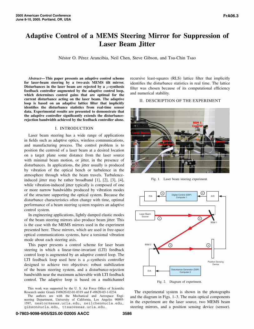
The experimental system is shown in the photographsand the diagram in Figs. 1–3. The main optical componentsin the experiment are the laser source, two MEMS beamsteering mirrors, and a position sensing device (sensor).

2005 American Control ConferenceJune 8-10, 2005. Portland, OR, USA

0-7803-9098-9/05/$25.00 ©2005 AACC

FrA06.3

3586

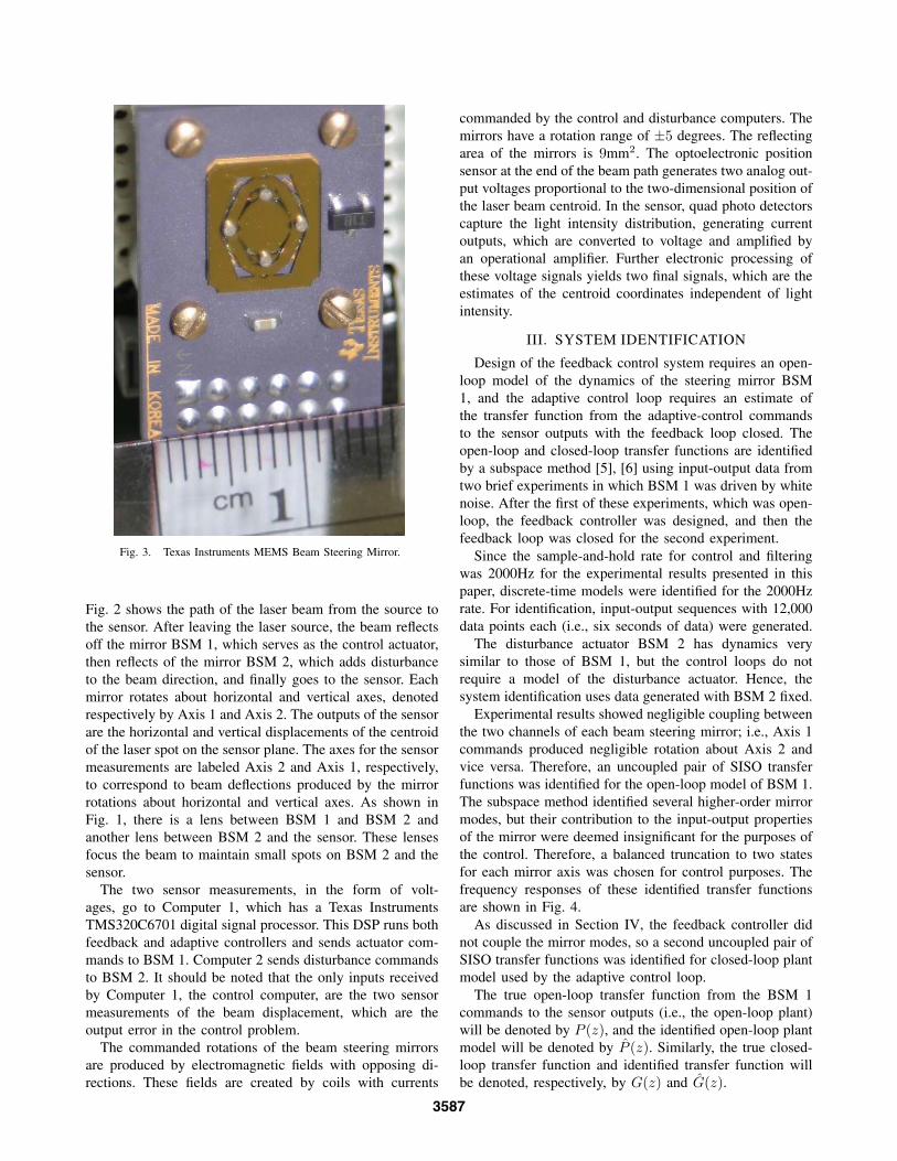
Fig. 3. Texas Instruments MEMS Beam Steering Mirror.

Fig. 2 shows the path of the laser beam from the source tothe sensor. After leaving the laser source, the beam reflectsoff the mirror BSM 1, which serves as the control actuator,then reflects of the mirror BSM 2, which adds disturbanceto the beam direction, and finally goes to the sensor. Eachmirror rotates about horizontal and vertical axes, denotedrespectively by Axis 1 and Axis 2. The outputs of the sensorare the horizontal and vertical displacements of the centroidof the laser spot on the sensor plane. The axes for the sensormeasurements are labeled Axis 2 and Axis 1, respectively,to correspond to beam deflections produced by the mirrorrotations about horizontal and vertical axes. As shown inFig. 1, there is a lens between BSM 1 and BSM 2 andanother lens between BSM 2 and the sensor. These lensesfocus the beam to maintain small spots on BSM 2 and thesensor.

The two sensor measurements, in the form of volt-ages, go to Computer 1, which has a Texas InstrumentsTMS320C6701 digital signal processor. This DSP runs bothfeedback and adaptive controllers and sends actuator com-mands to BSM 1. Computer 2 sends disturbance commandsto BSM 2. It should be noted that the only inputs receivedby Computer 1, the control computer, are the two sensormeasurements of the beam displacement, which are theoutput error in the control problem.

The commanded rotations of the beam steering mirrorsare produced by electromagnetic fields with opposing di-rections. These fields are created by coils with currents

commanded by the control and disturbance computers. Themirrors have a rotation range of ±5 degrees. The reflectingarea of the mirrors is 9mm2. The optoelectronic positionsensor at the end of the beam path generates two analog out-put voltages proportional to the two-dimensional position ofthe laser beam centroid. In the sensor, quad photo detectorscapture the light intensity distribution, generating currentoutputs, which are converted to voltage and amplified byan operational amplifier. Further electronic processing ofthese voltage signals yields two final signals, which are theestimates of the centroid coordinates independent of lightintensity.

III. SYSTEM IDENTIFICATION

Design of the feedback control system requires an open-loop model of the dynamics of the steering mirror BSM1, and the adaptive control loop requires an estimate ofthe transfer function from the adaptive-control commandsto the sensor outputs with the feedback loop closed. Theopen-loop and closed-loop transfer functions are identifiedby a subspace method [5], [6] using input-output data fromtwo brief experiments in which BSM 1 was driven by whitenoise. After the first of these experiments, which was open-loop, the feedback controller was designed, and then thefeedback loop was closed for the second experiment.

Since the sample-and-hold rate for control and filteringwas 2000Hz for the experimental results presented in thispaper, discrete-time models were identified for the 2000Hzrate. For identification, input-output sequences with 12,000data points each (i.e., six seconds of data) were generated.

The disturbance actuator BSM 2 has dynamics verysimilar to those of BSM 1, but the control loops do notrequire a model of the disturbance actuator. Hence, thesystem identification uses data generated with BSM 2 fixed.

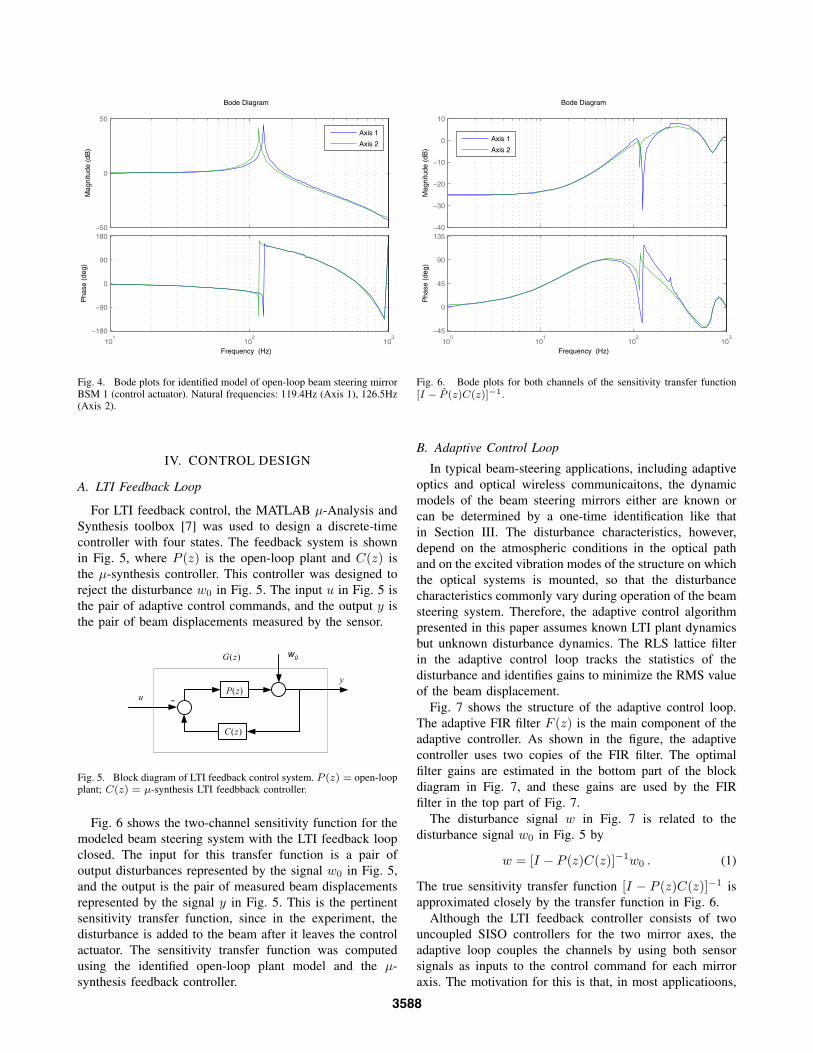
Experimental results showed negligible coupling betweenthe two channels of each beam steering mirror; i.e., Axis 1commands produced negligible rotation about Axis 2 andvice versa. Therefore, an uncoupled pair of SISO transferfunctions was identified for the open-loop model of BSM 1.The subspace method identified several higher-order mirrormodes, but their contribution to the input-output propertiesof the mirror were deemed insignificant for the purposes ofthe control. Therefore, a balanced truncation to two statesfor each mirror axis was chosen for control purposes. Thefrequency responses of these identified transfer functionsare shown in Fig. 4.

As discussed in Section IV, the feedback controller didnot couple the mirror modes, so a second uncoupled pair ofSISO transfer functions was identified for closed-loop plantmodel used by the adaptive control loop.

The true open-loop transfer function from the BSM 1commands to the sensor outputs (i.e., the open-loop plant)will be denoted by P (z), and the identified open-loop plantmodel will be denoted by P (z). Similarly, the true closed-loop transfer function and identified transfer function willbe denoted, respectively, by G(z) and G(z).

3587

−50

0

50

Mag

nitu

de (

dB)

101

102

103

−180

−90

0

90

180

Pha

se (

deg)

Bode Diagram

Frequency (Hz)

Axis 1

Axis 2

Fig. 4. Bode plots for identified model of open-loop beam steering mirrorBSM 1 (control actuator). Natural frequencies: 119.4Hz (Axis 1), 126.5Hz(Axis 2).

IV. CONTROL DESIGN

A. LTI Feedback Loop

For LTI feedback control, the MATLAB µ-Analysis andSynthesis toolbox [7] was used to design a discrete-timecontroller with four states. The feedback system is shownin Fig. 5, where P (z) is the open-loop plant and C(z) isthe µ-synthesis controller. This controller was designed toreject the disturbance w0 in Fig. 5. The input u in Fig. 5 isthe pair of adaptive control commands, and the output y isthe pair of beam displacements measured by the sensor.

)(zP

)(zG

)(zC

-u

y

w0

Fig. 5. Block diagram of LTI feedback control system. P (z) = open-loopplant; C(z) = µ-synthesis LTI feedbback controller.

Fig. 6 shows the two-channel sensitivity function for themodeled beam steering system with the LTI feedback loopclosed. The input for this transfer function is a pair ofoutput disturbances represented by the signal w0 in Fig. 5,and the output is the pair of measured beam displacementsrepresented by the signal y in Fig. 5. This is the pertinentsensitivity transfer function, since in the experiment, thedisturbance is added to the beam after it leaves the controlactuator. The sensitivity transfer function was computedusing the identified open-loop plant model and the µ-synthesis feedback controller.

−40

−30

−20

−10

0

10

Mag

nitu

de (

dB)

100

101

102

103

−45

0

45

90

135

Pha

se (

deg)

Bode Diagram

Frequency (Hz)

Axis 1

Axis 2

Fig. 6. Bode plots for both channels of the sensitivity transfer function[I − P (z)C(z)]−1.

B. Adaptive Control Loop

In typical beam-steering applications, including adaptiveoptics and optical wireless communicaitons, the dynamicmodels of the beam steering mirrors either are known orcan be determined by a one-time identification like thatin Section III. The disturbance characteristics, however,depend on the atmospheric conditions in the optical pathand on the excited vibration modes of the structure on whichthe optical systems is mounted, so that the disturbancecharacteristics commonly vary during operation of the beamsteering system. Therefore, the adaptive control algorithmpresented in this paper assumes known LTI plant dynamicsbut unknown disturbance dynamics. The RLS lattice filterin the adaptive control loop tracks the statistics of thedisturbance and identifies gains to minimize the RMS valueof the beam displacement.

Fig. 7 shows the structure of the adaptive control loop.The adaptive FIR filter F (z) is the main component of theadaptive controller. As shown in the figure, the adaptivecontroller uses two copies of the FIR filter. The optimalfilter gains are estimated in the bottom part of the blockdiagram in Fig. 7, and these gains are used by the FIRfilter in the top part of Fig. 7.

The disturbance signal w in Fig. 7 is related to thedisturbance signal w0 in Fig. 5 by

w = [I − P (z)C(z)]−1w0 . (1)

The true sensitivity transfer function [I − P (z)C(z)]−1 isapproximated closely by the transfer function in Fig. 6.

Although the LTI feedback controller consists of twouncoupled SISO controllers for the two mirror axes, theadaptive loop couples the channels by using both sensorsignals as inputs to the control command for each mirroraxis. The motivation for this is that, in most applicatioons,

3588

the jitter signals in different directions are at least partiallycorrelated. Therefore, the adaptive controller design hereuses all available sensor information to suppress beam jitterin each direction. he block diagram to generate the adaptivecontrol signal u.

Closed Loop Plant

)(zG

Closed Loop Plant Model

)(ˆ zG

+

+

Copy of

)(zF

output

+

-

edisturbanc

u

Closed Loop Plant ModelLattice Filter)(zF )(ˆ zGz

1

z

1

Adaptive Lattice AlgorithmComputes Gains for

)(zF+ Error

m

w

w

yv

-

Fig. 7. Block diagram of adaptive control system.

BackwardBlockn=1

z-1 ForwardBlockn=1

( )t

( )t( )t

BackwardBlockn=2

z-1 ForwardBlockn=2

BackwardBlockn=N

z-1 ForwardBlockn=N

Fig. 8. Block diagram of FIR lattice filter.

Both copies of the FIR filter, as well as the RLS algorithmthat estimates the optimal gains, have a lattice structure. Thelattice realization of the FIR filter of order N consists ofN identical stages cascaded as in Fig. 8. The details ofthe algorithms represented by the blocks in Fig. 8 and theRLS algorithm are beyond the scope of this paper. Thesealgorithms are reparameterized versions of algorithms in[8]. The current parameterization of the lattice algorithmsis optimized for indefinite real-time operation. The currentlattice filter maintains the channel orthogonalization in [8],which is essential to numerical stability in multichannelapplications, and the unwindowed characteristic of the lat-tice filter in [8], which is essential to rapid convergence.The inputs η and ξ to both copies of the lattice filter areconstructed from the signal w in Fig. 7. The output ε ofthe copy of the lattice filter in the top part of Fig. 7 is theadaptive control signal.

V. EXPERIMENTAL RESULTS

Two typical sets of experimental results are shown inFigs. 9 and 10. In these experiments, the sample-and-hold

rate for control and filtering was 2000Hz. The lattice-filterorder N = 16 was used for these results. For these and othersimilar experiments, the performance of the adaptive loopwas evaluated with several lattice-filter orders. The order16 yielded better performance than lower orders, but ordershigher than 16 yielded no further improvement.

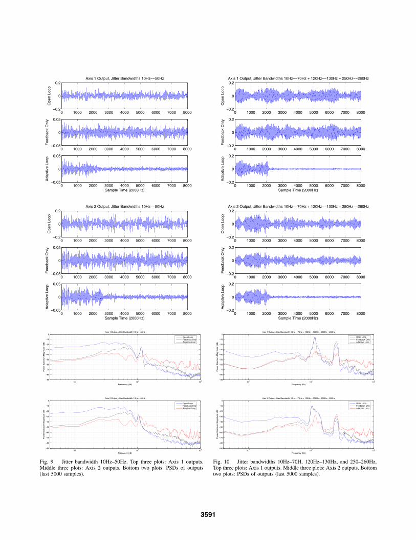
For the experiments summarized in Fig. 9, the samedisturbance command sequence was sent to each axis ofthe disturbance actuator BSM 2. This disturbance commandsignal was created by passing white noise through a fourth-order Butterworth bandpass filter with bandwidth 10Hz–50Hz. Fig. 9 shows output sequences (i.e., measured beamdisplacements at the sensor) for (1) an open-loop experi-ment, (2) an experiment with only the LTI feedback loopclosed, and (3) an experiment in which the adaptive loopstarts after 2000 samples (2 sec). The last two plots inFig. 9 show the PSDs of the last 5000 points in each outputsequence.

The open-loop output is just the disturbance. As thePSDs in Fig. 9 show, the disturbance contains significantpower not only in the 10H–50Hz range but also around120Hz due the the lightly damped modes of the disturbanceactuator. Since the steering mirror BSM 2 is not controlledwith a feeback loop, the vibration modes of this mirror areprominent in the disturbance sequences added to the laserbeam.

In the experiments where the adaptive loop is closed,only the LTI feedback loop was closed for the first 2000samples. Then the RLS lattice filter started running and ranfor 50 learning steps (0.025 sec) before the adaptive controlloop was closed at step 2051. Depending on the nature ofthe disturbance at the time when the adaptive control loopwas closed, the effect of the adaptive loop on the output isseen almost immediately, as in data for Axis 1 in Fig. 9, oras much as 0.25 sec later, as in data for Axis 2 in Fig. 9.

The PSDs show that, as predicted by Fig. 6, the LTIµ-synthesis feedback loop significantly reduces the jitterbelow about 80Hz but has little effect beyond that. ThePSDs also show that the adaptive loop yields significantjitter reduction between about 70Hz and 130Hz, therebyextending the bandwidth of the feedback loop. This ex-tended jitter reduction in the higher frequencies accounts forthe significant reduction in the RMS values of the outputsevidenced by the last 5000 samples in the time series.

Another noteworthy point in the PSDs in Fig. 9 is thatboth the feedback loop and the adaptive loop amplifyjitter above 200Hz, and this high-frequency amplificationis greater for the adaptive loop. Of course, the jitter poweris so low above 200Hz that the amplification in this ex-periment still leaves low high-frequency power. However,it might asked whether the adaptive loop would amplifyhigh-frequency jitter similarly if there were significant jitterpower about 200Hz. The next set of experiment resultsanswer this question.

For the experiments summarized in Fig. 10, two different

3589

but partially correlated disturbance commands were sentto BSM 2. These two tilt command sequences are thecomponents of the signal w0 in Figure 5. In the experiments,this signal had the form

w0 =

[4 11 2

] [v1

v2

](2)

where the sequences v1 and v2 were obtained by passingindependent white noise sequences through bandpass filters.The bandpass filter used to generate v1 was the sumof two Butterworth filters with bandwidths 120Hz–130Hzand 250Hz–260Hz. The filter used to generate v2 was aButterworth filter with bandwidth 10Hz–70Hz.

The PSDs in Fig. 10 show that, again as predicted byFig. 6, the LTI feedback loop significantly reduces the jitterbelow about 80Hz, has no significant effect in the bandwidth100Hz–130Hz, where most of the jitter power lies, butsignificantly amplifies the Axis-1 jitter in the bandwidth250Hz–260Hz. In this case, as in Fig. 9, the adaptive loopsignificantly reduces the jitter between 70Hz and 130Hz.However, as opposed to the case in Fig. 9, the PSDs inFig. 10 show that the adaptive loop significantly reducesthe Axis-1 jitter in the bandwidth 250Hz–260Hz and onlyslightly amplifies the Axis-2 jitter in this bandwidth abovethe level to which the feedback loop raised it. The differencebetween the way the adaptive loop handles the 250Hz–260Hz jitter in the two axes results from the fact that theopen-loop jitter in this bandwidth is approximately 20dbhigher for Axis 1 than for Axis 2.

Of course, the optimal FIR filter in the adaptive loop isdifferent for the two experiments. In each case, the RLSlattice identifies the filter that is optimal for the particulardisturbance. The rule that determines the frequency rangeswhere the adaptive loop reduces or amplifies power isthat the adaptive filter generally whitens the residual-errorsequence. This means accepting some power increase inbandwidths where the open-loop jitter is small to be ableto achieve large reductions in the dominant jitter power.

VI. CONCLUSIONS

This paper has presented a method for adaptive suppres-sion of jitter in laser beams. The method has been demon-strated by results from beam steering experiment employingtwo-axis MEMS tilt mirrors. Disturbances in the laser beamare rejected by a µ-synthesis feedback controller augmentedby the adaptive control loop, which determines control gainsthat are optimal for the current disturbance acting on thelaser beam. The adaptive loop is based on an adaptive latticefilter that implicitly identifies the disturbance statistics fromreal-time sensor data. Experimental results demonstrate thatthe adaptive controller significantly extends the disturbancerejection bandwidth achieved by the feedback controlleralone. This adaptive scheme is most suited to reject jitterwhere the statistics of the disturbance vary from time to timedue to changes in environmental conditions. The adaptivelattice filter is able to perform high order and multi-channel

RLS (recursive-least-squares) computation in real-time athigh sampling rates, and RLS yields faster convergence tooptimal gains than does LMS (least mean squares), whichis more commonly used in adaptive disturbance-rejectionapplications.

VII. ACKNOWLEDGMENTS

The authors are indebted to Texas Instruments for pro-viding the TALP1000A MEMS steering mirrors used in thisresearch.

REFERENCES

[1] M. C. Roggemann and B. Welsh, Imaging through Turbulence. NewYork: CRC, 1996.

[2] R. K. Tyson, Principles of Adaptive Optics. New York: AcademicPress, 1998.

[3] B. L. Ellerbroek, “First-order performance evalution of adaptive opticssystems for atmospheric turbulence compensation in extended field-of-view astronomical telescopes,” J. Opt. Soc. Am. A, vol. 11, pp.783–805, 1994.

[4] R. Q. Fugate and B. L. Ellerbroek et al., “Two generations of laserguide star adaptive optics experiments at the starfire optical range,” J.Opt. Soc. Am. A, vol. 11, pp. 310–324, 1994.

[5] Y. M. Ho, G. Xu, and T. Kailath, “Fast identification of state-spacemodels via exploitation of displacement structure,” IEEE Transactionson Automatic Control, vol. 39, no. 10, pp. 2004–2017, October 1994.

[6] P. Van Overschee and B. De Moor, Subspace Identification for LinearSystems. Norwell, MA: Kluwer Academic Publishers, 1996.

[7] G. J. Balas, J. C. Doyle, K. Glover, A. Packard, and R. Smith, µ-Analisis and Synthesis Toolbox. Mathworks.

[8] S.-B. Jiang and J. S. Gibson, “An unwindowed multichannel latticefilter with orthogonal channels,” IEEE Transactions on Signal Pro-cessing, vol. 43, no. 12, pp. 2831–2842, December 1995.

3590

0 1000 2000 3000 4000 5000 6000 7000 8000−0.2

0

0.2

Ope

n Lo

op

Axis 1 Output, Jitter Bandwidths 10Hz−−50Hz

0 1000 2000 3000 4000 5000 6000 7000 8000−0.05

0

0.05

Fee

dbac

k O

nly

0 1000 2000 3000 4000 5000 6000 7000 8000−0.05

0

0.05

Ada

ptiv

e Lo

op

Sample Time (2000Hz)

0 1000 2000 3000 4000 5000 6000 7000 8000−0.2

0

0.2

Ope

n Lo

op

Axis 2 Output, Jitter Bandwidths 10Hz−−50Hz

0 1000 2000 3000 4000 5000 6000 7000 8000−0.05

0

0.05

Fee

dbac

k O

nly

0 1000 2000 3000 4000 5000 6000 7000 8000−0.05

0

0.05

Ada

ptiv

e Lo

op

Sample Time (2000Hz)

101

102

103

−90

−80

−70

−60

−50

−40

−30

−20

−10

0

Frequency (Hz)

Pow

er S

pect

rum

Mag

nitu

de (

dB)

Axis 1 Output, Jitter Bandwidth 10Hz−−50Hz

Open LoopFeedback OnlyAdaptive Loop

101

102

103

−90

−80

−70

−60

−50

−40

−30

−20

−10

0

Frequency (Hz)

Pow

er S

pect

rum

Mag

nitu

de (

dB)

Axis 2 Output, Jitter Bandwidth 10Hz−−50Hz

Open LoopFeedback OnlyAdaptive Loop

Fig. 9. Jitter bandwidth 10Hz–50Hz. Top three plots: Axis 1 outputs.Middle three plots: Axis 2 outputs. Bottom two plots: PSDs of outputs(last 5000 samples).

0 1000 2000 3000 4000 5000 6000 7000 8000−0.2

0

0.2

Ope

n Lo

op

Axis 1 Output, Jitter Bandwidths 10Hz−−70Hz + 120Hz−−130Hz + 250Hz−−260Hz

0 1000 2000 3000 4000 5000 6000 7000 8000−0.2

0

0.2

Fee

dbac

k O

nly

0 1000 2000 3000 4000 5000 6000 7000 8000−0.2

0

0.2

Ada

ptiv

e Lo

op

Sample Time (2000Hz)

0 1000 2000 3000 4000 5000 6000 7000 8000−0.2

0

0.2

Ope

n Lo

op

Axis 2 Output, Jitter Bandwidths 10Hz−−70Hz + 120Hz−−130Hz + 250Hz−−260Hz

0 1000 2000 3000 4000 5000 6000 7000 8000−0.2

0

0.2

Fee

dbac

k O

nly

0 1000 2000 3000 4000 5000 6000 7000 8000−0.2

0

0.2

Ada

ptiv

e Lo

op

Sample Time (2000Hz)

101

102

103

−90

−80

−70

−60

−50

−40

−30

−20

−10

0

Frequency (Hz)

Pow

er S

pect

rum

Mag

nitu

de (

dB)

Axis 1 Output, Jitter Bandwidth 10Hz−−70Hz + 120Hz−−130Hz + 250Hz−−260Hz

Open LoopFeedback OnlyAdaptive Loop

101

102

103

−90

−80

−70

−60

−50

−40

−30

−20

−10

0

Frequency (Hz)

Pow

er S

pect

rum

Mag

nitu

de (

dB)

Axis 2 Output, Jitter Bandwidth 10Hz−−70Hz + 120Hz−−130Hz + 250Hz−−260Hz

Open LoopFeedback OnlyAdaptive Loop

Fig. 10. Jitter bandwidths 10Hz–70H, 120Hz–130Hz, and 250–260Hz.Top three plots: Axis 1 outputs. Middle three plots: Axis 2 outputs. Bottomtwo plots: PSDs of outputs (last 5000 samples).

3591