Adaptive Critic Based Optimal Kinematic Control for a RobotManipulator

Aiswarya Menon1, Ravi Prakash2, Laxmidhar Behera3, Senior Member, IEEE

Abstract— This paper is concerned with the optimal kine-matic control of a robot manipulator where the robot endeffector position follows a task space trajectory. The jointsare actuated with the desired velocity profile to achieve thistask. This problem has been solved using a single networkadaptive critic (SNAC) by expressing the forward kinematicsas input affine system. Usually in SNAC, the critic weights areupdated using back propagation algorithm while little attentionis given to convergence to the optimal cost. In this paper, wepropose a critic weight update law that ensures convergenceto the desired optimal cost while guaranteeing the stability ofthe closed loop kinematic control. In kinematic control, therobot is required to reach a specific target position. This hasbeen solved as an optimal regulation problem in the context ofSNAC based kinematic control. When the robot is required tofollow a time varying task space trajectory, then the kinematiccontrol has been framed as an optimal tracking problem.For tracking, an augmented system consisting of trackingerror and reference trajectory is constructed and the optimalcontrol policy is derived using SNAC framework. The stabilityand performance of the system under the proposed novelweight tuning law is guaranteed using Lyapunov approach.The proposed kinematic control scheme has been validated insimulations and experimentally executed using a real six degreesof freedom (DOF) Universal Robot (UR) 10 manipulator.

I. INTRODUCTION

Modern robotic systems are becoming complex as thedegrees of freedom are increasing to address the complexapplication scenario such as agriculture, health-care andware-house automation. A mobile manipulator with Shadowhand mounted on it has 28 degrees of freedom. The inversekinematic solution to such systems can not be solved analyt-ically. Thus neural and fuzzy neural network based schemeshave become popular to design kinematic control[1], [2], [3],[4]. These approaches can not learn the inverse kinematicswhile optimizing a global cost function. This is very im-portant when one deals with redundant manipulators. Oneof the approaches to design optimal kinematic control isto use the Hamilton-Jacobi-Bellman (HJB) formulation [5],[6]. The analytical solution of the HJB equation is still amajor challenge and as such these solutions are obtainedoff-line. The real time approximate solutions are known asapproximate dynamic programming and are presented in [7],[8], [9]. In these approaches, the framework uses two neuralnetworks - one for action and the other critic. Action networklearns to actuate an optimal policy while critic networkevaluates the cost function through learning.

All authors are with the Department of Electrical Engineering,Indian Institute of Technology, Kanpur, India-208016. Email id :1aiswarya@iitk.ac.in, 2ravipr@iitk.ac.in,3lbehera@iitk.ac.in

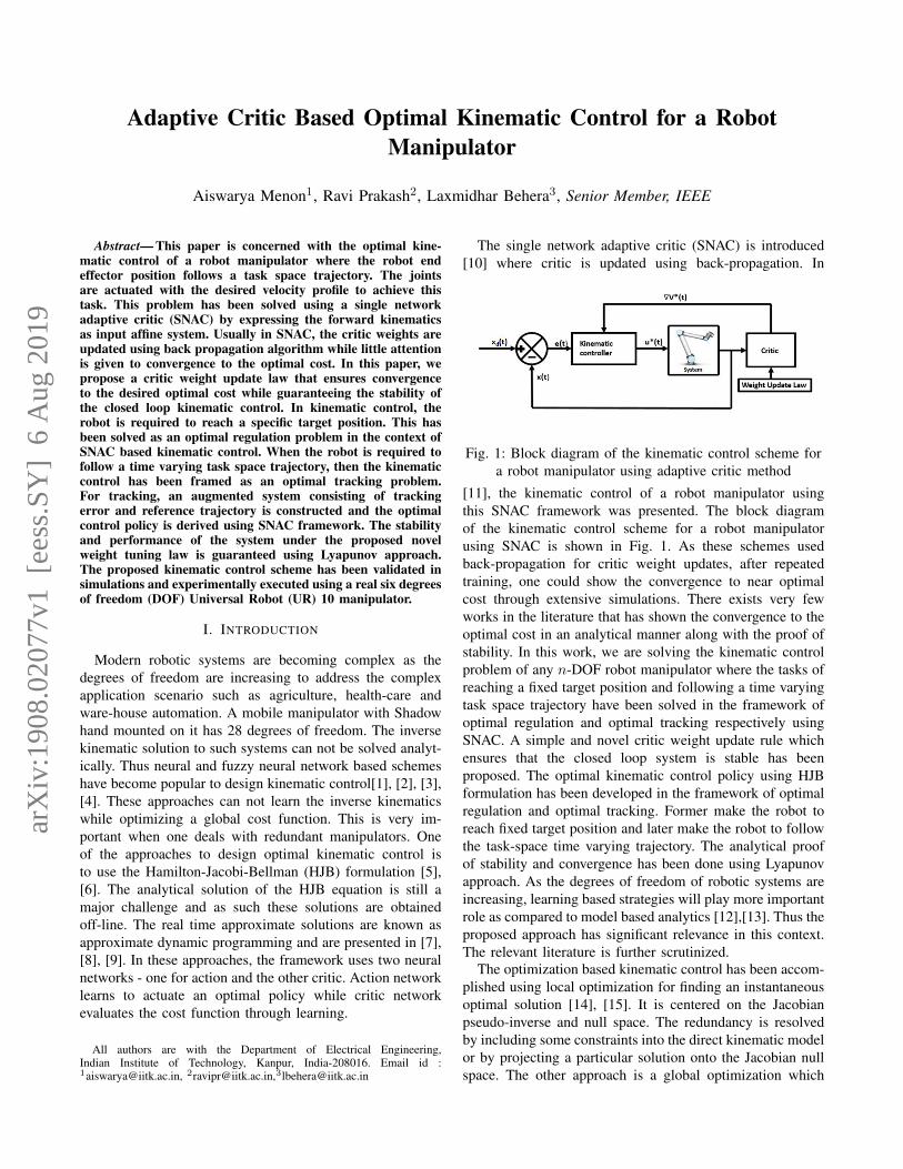
The single network adaptive critic (SNAC) is introduced[10] where critic is updated using back-propagation. In

Fig. 1: Block diagram of the kinematic control scheme fora robot manipulator using adaptive critic method

[11], the kinematic control of a robot manipulator usingthis SNAC framework was presented. The block diagramof the kinematic control scheme for a robot manipulatorusing SNAC is shown in Fig. 1. As these schemes usedback-propagation for critic weight updates, after repeatedtraining, one could show the convergence to near optimalcost through extensive simulations. There exists very fewworks in the literature that has shown the convergence to theoptimal cost in an analytical manner along with the proof ofstability. In this work, we are solving the kinematic controlproblem of any n-DOF robot manipulator where the tasks ofreaching a fixed target position and following a time varyingtask space trajectory have been solved in the framework ofoptimal regulation and optimal tracking respectively usingSNAC. A simple and novel critic weight update rule whichensures that the closed loop system is stable has beenproposed. The optimal kinematic control policy using HJBformulation has been developed in the framework of optimalregulation and optimal tracking. Former make the robot toreach fixed target position and later make the robot to followthe task-space time varying trajectory. The analytical proofof stability and convergence has been done using Lyapunovapproach. As the degrees of freedom of robotic systems areincreasing, learning based strategies will play more importantrole as compared to model based analytics [12],[13]. Thus theproposed approach has significant relevance in this context.The relevant literature is further scrutinized.

The optimization based kinematic control has been accom-plished using local optimization for finding an instantaneousoptimal solution [14], [15]. It is centered on the Jacobianpseudo-inverse and null space. The redundancy is resolvedby including some constraints into the direct kinematic modelor by projecting a particular solution onto the Jacobian nullspace. The other approach is a global optimization which

arX

iv:1

908.

0207

7v1

[ee

ss.S

Y]

6 A

ug 2

019

uses an integral type performance index along the wholetrajectory [16], [17]. The redundancy resolution is convertedto an optimal control problem with the necessary conditionsof optimality given by the Pontryagin’s principle or by theoptimal control theory. Both of the aforementioned methodsare suboptimal and require the pseudo-inversion of Jacobiancontinuously over time which is computationally expensiveand suffers from local instability problems [18], [19], [20].

Existing approach towards following a time varying taskspace trajectory optimally is to find the feedforward termusing the dynamics inversion concept and the feedback termby solving an HJB equation [21]. However, such solution isonly near optimal because of the feedforward term. There-fore by using an augmented system dynamics consisting offeedback tracking error and reference trajectory and using itto solve the HJB equation results in an optimal control lawwhich is a combination of feedforward and feedback controlinputs [22].

The remainder of this paper is organised as follows. Prob-lem formulation for optimal kinematic control is presentedin Section II. In Section III and IV detailed mathematicalderivation for the control scheme along with stability proof ispresented. In Section V, various simulation and experimentalresults for kinematic motion control of a 6-DOF roboticmanipulator are evaluated with comparison with the state-of-the-art kinematic control solutions. This paper is finallyconcluded in Section VI.

II. PROBLEM FORMULATION

The forward kinematics of a manipulator involves a non-linear transformation from Joint space to Cartesian space asdescribed by:

x(t) = f(θ(t)) (1)

where, x(t) ∈ Rn×1 describes the position and orientationof end effector in workspace at time t, θ(t) ∈ Rm×1 eachelement of which describes the joint angle in the joint spaceat time t, and f(.) is the non linear mapping. Because of non-linearity and redundancy of mapping, it is usually difficultto directly get θ(t) for desired x(t) = xd(t), where xd(t) isthe desired end effector position. By contrast, the mappingfrom joint space to cartesian space at velocity level is affinemapping. Taking time derivative on both sides of (1) gives:

x(t) = Jθ(t) (2)

where, J = ∂f∂θ ∈ Rn×m is the Jacobian matrix of f(.).

In this paper we focus on design of angular speed of themanipulator which serves as an input to the tracking controlloop for robot control. Then the robot manipulator kinematicscan be rewritten by replacing θ(t) by u(t):

x(t) = Ju(t) (3)

Thus, we get the dynamics of the system as above. In thispaper we propose to solve for an optimal control inputu(t) for a robot manipulator described by (3), such that thetracking error given by,

e(t) = x(t)− xd(t) (4)

for a given reference trajectory xd(t), reduces to zero withtime.

III. OPTIMAL REGULATION

In this section, we address the optimal kinematic controlof a robot manipulator, where the robot end effector has toreach a fixed target position. This is framed as an optimalregulation problem. In the context of kinematic control,optimal regulation means that the robot is made to reacha fixed target position following an optimal trajectory. Thistrajectory is generated by actuating the desired optimalcontrol policy.

Let xd(t) ∈ Rn×1 be the desired end effector position.Differentiating (4) with respect to time, error dynamics ofthe system is obtained as,

e = x(t) = Ju(t) (5)

A. Formulation of control policy

The infinite horizon HJB cost function for (5) is given by,

V (e(t)) =

ˆ ∞t

e(t)TQe(t) + u(t)TRu(t)dt (6)

where, Q ∈ Rn×n and R ∈ Rm×m are positive definitedesign matrices. The control input needs to be admissible sothat the cost function equation (6) is finite. The Hamiltonianfor the this cost function with the admissible control inputu(t) is,

H(e(t), u(t),∇V (t)) =∇V ∗T e(t) + e(t)TQe(t)

+ u(t)TRu(t)(7)

Here, ∇V ∗ is the gradient of the cost function V (e(t)) withrespect to e(t). The optimal control input which minimizesthe cost function (6) also minimizes the Hamiltonian (7).Therefore, the optimal control is found by solving thefollowing condition ∂H(e,u,∇V )

∂u = 0 and obtained to be

u∗(e) =−1

2R−1JT∇V ∗(e) (8)

Then, HJB equation may be re-written as follows,

0 = ∇V ∗T e(t) + e(t)TQe(t) + u∗(t)TRu∗(t) (9)

with the cost function V ∗(0) = 0.

B. Neural Network control design

By using the universal approximation property, V ∗(e(t))is constructed by a single hidden layer neural network witha non-linear activation function:

V ∗(e(t)) = WTc σc(e) + εc (10)

where, Wc ∈ Rl, is the constant target NN weight vector,σc ∈ Rl is the activation function output, l is the number ofhidden neurons and εc is the function reconstruction error.The target NN vector and reconstruction errors are assumedto be upper bounded according to ‖Wc ‖≤ λWc

and ‖ εc ‖≤λε.

∇V ∗ = ∇σTc Wc +∇εc (11)

Approximate optimal cost function and its gradient is givenby

V ∗ = WcTσc(e) (12)

∇V ∗ = ∇σTc Wc (13)

where, Wc is the NN estimate of target weight vector Wc.Using (8) and (11), the optimal control law can be writtenas:

u∗(e) =−1

2R−1JT (∇σTCWc+∇εc) (14)

Considering (8) and (13), estimated optimal control law is:

u∗(e) =−1

2R−1JT∇σTc Wc (15)

The modified error dynamics using (15) is,

e = −1

2JR−1JT∇σTc Wc (16)

Before proposing the critic weight tuning law and stabilityproofs, following assumptions need to be made:

Assumption 1: For the system represented by its error dy-namics (5), with cost function (6), let Js(e) be a continuouslydifferentiable Lyapunov function candidate satisfying,

˙Js(e) = ∇Js(e)T e < 0 (17)

Then, there exists a positive definite matrix, M ∈ Rn×nensuring,

∇Js(e)T e = −∇Js(e)TM∇Js(e) ≤ −λmin(M) ‖ ∇Js(e) ‖2(18)

During the implementation, Js(e) can be obtained byselecting a polynomial with respect to the vector e, suchas Js(e) = 1

2eT e.

Remark 1: Based on the result of [23], the closed loopdynamics with optimal control law can be bounded by afunction of the system state. In such situations, it can beasssumed that ‖ F (e) + G(e)(u∗) ‖≤ η ‖ ∇Js(e) ‖ withη > 0, ‖ ∇Js(e) ‖T ‖ F (e) + G(e)(u∗) ‖≤ η ‖ ∇Js(e) ‖2.Combining (17) with the fact given, λmin ‖ ∇Js(e) ‖2≤∇Js(e)TM∇Js(e) ≤ λmax(M) ‖ ∇Js(e) ‖2, it impliesthat assumption 1 holds.

Moving on, a simple and novel critic weight tuning lawis proposed.

˙Wc = α∇σcJR−1JT∇Js(e) (19)

where, α is the learning rate of critic network and Js(e) =12eT e.By using this weight tuning law, stability and per-

formance is guaranteed theoretically using the Lyapunovapproach.

C. Stability Analysis

In this section, the stability of the system for optimalregulation is investigated.Assumption 2: The Jacobian matrix is bounded as ‖ J(θ) ‖≤λJ ,where λJ is a positive constant. Here, the control coef-ficient matrix is the Jacobian matrix. Also, ∇σc,∇εc arebounded as ‖ ∇σc ‖≤ λσ and ‖ ∇εc ‖≤ λ∇ε where λσ and

λ∇ε are positive constants.The Lyapunov candidate function is selected as,

L(t) =1

4αWc

TWc + Js(e) (20)

L(t) =1

2αWc

T ˙Wc +∇JTs e (21)

where, W = Wc − Wc. Using (19),

L(t) =−1

2Wc

T∇σJR−1JT∇Js +∇JTs (e) (22)

The system error dynamics of the system for the optimalcontrol law is e∗ = Ju∗. Using the control laws (14) and(15),

e∗ − e =J(u∗ − u∗) = −1

2JR−1JT (∇σTc Wc +∇εc)

(23)Using (23) in (22) and on simplification,

L(t) = ∇JTs e∗ +1

2∇JTs JR−1JT∇εc (24)

Applying Assumption 1 and Assumption 2 here

L ≤ −λmin(M) ‖ ∇Js ‖2 +1

2‖ ∇Js ‖ λ2

J ‖ R−1 ‖ λ∇ε(25)

From (25), the following inequality may be derived:

‖ ∇Js ‖≥1

2λmin(M)λ2J ‖ R−1 ‖ λ∇ε (26)

With the above condition to be true, L ≤ 0 and the systemis stable in the sense of Lyapunov implying that Wc and eare both bounded. It may be expressed as : ‖ Wc ‖≤ λWc

.It may be also observed that the estimated optimal con-

troller (15) converges to a neighborhood of the optimalfeedback controller (14) with a finite bound λu as,

‖ u∗(e)− u∗(e) ‖≤ 1

2‖ R−1 ‖ λJ(λσλWc

+ λ∇ε)∆= λu

(27)Hence, it may be concluded that the instantaneous costfunction V (e, u, t) = e(t)TQe(t) + u(t)TRu(t) is alsobounded.

Taking time derivative of (24),

L = eT e∗ + eT e∗ +1

2eTJR−1JT∇εc + eT JR−1JT∇εc+

1

2eTJR−1JT∇2εce

(28)Remark 2:All the terms in L can be shown to be bounded.

It may be observed that L is bounded and Barbalat’sLemma [24] can be invoked to conclude the asymtoticstability of the system and convergence of the parameterestimation error and the weight estimation errors towardszero. In other words, it ensures that Wc → 0.

IV. OPTIMAL TRACKING CONTROL

In this section, the kinematic control of a robot manipula-tor following a time varying task space trajectory is solvedin the framework of optimal tracking.

A. Formation of Augmented System

Let the time varying reference trajectory, denoted byxd(t) ∈ Rn be possessing the dynamics

xd(t) = ϕ(xd(t)) (29)

with the initial condition xd(0) = xd0, where, ϕ(xd(t)) is aLipschitz continuous function satisfying ϕ(0) = 0. Let thetrajectory tracking error be e(t) = x(t) − xd(t) with theinitial condition e(0) = e0 = x0 − xd0. Considering (3) and(29), the tracking error dynamics is:

e(t) = −ϕ(xd(t)) + Ju(t) (30)

Next, an augmented system is constructed as in [22],in theform ξ(t) = [e(t)T , xd(t)

T ]T ∈ R2n with initial conditionξ(0) = ξ0 = [eT0 , xd

T0 ]T . The augmented dynamics based on

(29) and (30) can be formulated as:

ξ(t) = F (ξ(t)) +G(ξ(t))u(t) (31)

where, F(.) and G(.) are the new system matrices.

B. Formulation of Control Policy

The infinite horizon HJB cost function for the system in(31) is given by,

V (ξ(t)) =

ˆ ∞t

ξ(t)T Qξ(t) + u(t)TRu(t).dt (32)

where, Q = diag{Q, 0n×n}. Q ∈ Rn×n and R ∈ Rm×mare positive definite matrices. The control input must beadmissible so that cost function given by (32) is finite.

Applying the same methods of solving as in Section III-A,the control policy is obtained as,

u∗(ξ) =−1

2R−1G(ξ)T∇V ∗(ξ) (33)

C. Neural Network control design

Here, V ∗(ξ(t)) is constructed by a single hidden layerneural network with a non-linear activation function:

V ∗(ξ(t)) = WTc φc(ξ) + εc (34)

where, Wc ∈ Rp, is the ideal weight, ‖Wc ‖≤ λWc , φc ∈ Rpis the activation function output, p is the number of hiddenneurons and εc is the function approximation error.

Using the same approach as in Section III-B, optimalcontrol law and approximate control law may be obtainedas,

u∗(ξ) =−1

2R−1G(ξ)T (∇φTCWc+∇εc) (35)

u∗(ξ) =−1

2R−1G(ξ)T∇φTc Wc (36)

Applying (36) into the augmented system dynamics (31),ξ(t) = F (ξ) +G(ξ)u∗(t) can be formulated as:

ξ = F (ξ)− 1

2G(ξ)R−1G(ξ)T∇φTc Wc (37)

The weight update law proposed for the critic of optimaltracking control is,

˙Wc = α∇φcG(ξ)R−1G(ξ)T∇Js(ξ) (38)

where, α is the learning rate of critic network and Js(ξ) =12ξT ξ.Remark 3: Assumption 1 and Remark 1 holds here.

The augmented system states shall replace the system errorstates as follows ; For the augmented system (31), withcost function (32), let Js(ξ) be a continuously differentiableLyapunov function candidate satisfying,

Js(ξ) = ∇Js(ξ)T ξ < 0 (39)

Then,there exists a positive definite matrix, M ∈R2n×2nensuring,

∇Js(ξ)T ξ = −∇Js(ξ)TM∇Js(ξ) ≤ −λmin(M) ‖ ∇Js(ξ) ‖2(40)

During the implementation,Js(ξ) = 12ξT ξ.

D. Stability AnalysisIn this section, the stability of the system is investigated.Remark 4: Assumption 2 holds here. However, the control

coefficient matrix is modified. The assumption ‖ G(ξ) ‖≤λg , where λg is a positive constant shall be used.Lyapunov function,

L(t) =1

4αWc

TWc + Js(ξ) (41)

L(t) =1

2αWc

T ˙Wc +∇JTs ξ (42)

Using the similar approach as in Section III-C,

L(t) = ∇JTs ξ∗ +1

2∇JTs G(ξ)R−1G(ξ)T Wc (43)

Applying the Remark 3 and Remark 4 here

L ≤ −λmin(M) ‖ ∇Js ‖2 +1

2‖ ∇Js ‖ λ2

g ‖ R−1 ‖ λ∇ε(44)

From this, we observe that if the condition below holds, then,L(t) ≤ 0 is negative semidefinite implying that the systemis stable in the sense of Lyapunov.

‖ ∇Js ‖≥1

2λmin(M)λ2g ‖ R−1 ‖ λ∇ε (45)

Hence, Wc and ξ are both bounded. It may be expressedas : ‖ Wc ‖≤ λWc

Also,

‖ u∗(ξ)− u∗(ξ) ‖≤ 1

2‖ R−1 ‖ λg(λσλWc

+ λ∇εc)∆= λu

(46)It may be noted that estimated controller input converges tothe neighbourhood of the optimal control input as a finitebound λu exists just as in the case of regulation. It is alsoobserved that the cost function V (ξ, u, t) = ξ(t)T Qξ(t) +u(t)Tu(t) is also bounded.

Using the same approach as in Section III-C, it maybe shown that L is bounded. Recalling Barbalat’s Lemma[25], it may be concluded that the system is stable and thatthe parameter estimation error and weight estimation errorconverge to zero.

Fig. 2: Hardware Setup

V. RESULTS AND DISCUSSION

In this section, we consider the numerical simulations fol-lowed by real time experimental validations on a real 6 DOFUR 10 robot manipulator to demonstrate the effectiveness ofthe proposed kinematic control.

A. Experimental SetupOur experimental setup shown in Fig. 2 consists of a

UR10 robot manipulator with its controller box/internalcomputer and a host PC/external computer. The UR10 robotmanipulator is a 6 DOF robot arm designed to safely workalongside and in collaboration with a human. This arm canfollow position commands like a traditional industrial robot,as well as take velocity commands to apply a given velocityin/around a specified axis. The low level robot controller is aprogram running on UR10’s internal computer broadcastingrobot arm data , receiving and interpreting the commands andcontrolling the arm accordingly. There are several optionsfor communicating with the robot low level controller tocontrol the robot including the teach pendent or opening aTCP socket (C++/Python) on a host computer. We used opensource C++ based UrDriver wrapper class integrated withROS on a host PC to implement our proposed velocity basedkinematic control scheme. The host PC streams joint velocitycommands via URScript to the robot real time interface overEthernet at 125Hz. The driver was configured with necessaryparameters like IP address of the robot at startup using ROSparameter server.B. Reaching a Fixed Position

Simulations are first performed to verify the kinematiccontrol of the robot manipulator to reach a fixed positionusing the control law expressed in Equation (15). A typicalsimulation run generated with a random seed pose (θ0 =[−0.51−1.041.48−1.82−1.45−1.62]rad) to a fixed targetpose [−0.658, 0.626, 0.407]m in cartesian space is shown inFigure 3(a).The weights were initialized randomly and α =αinitial(tanh(n−k))+αfinal, where, n=50, k=time instance,

αinitial = 100 and αfinal = 150.The predicted cost functionwas: w1e

21 + w2e1e2 + w3e1e3 + w4e

22 + w5e2e3 + w6e

23

C. Following a Time Varying Reference Trajectory

In this section, the kinematic control of the robot ma-nipulator to follow a time varying reference trajectory isvalidated. Simulations are first performed using the controllaw derived in Equation (36). A typical simulation generatedwith a random seed pose (θ0 = [−0.51− 1.041.48− 1.82−1.45 − 1.62]rad) and following a time varying referencetrajectory moving at an angular speed of 0.075 rad/s alonga circle centered at [−0.7, 0, 0.5]m with a radius of 0.2m isshown in Figure 3(e). Weights were initialized randomly andα = αinitial(tanh(n − k)) + αfinal, where, n=10, k=timeintance, αinitial = 20 and αfinal = 70. In this work, wetake the predicted cost to be:w1ξ

21 +w2ξ1ξ2 +w3ξ1ξ3 +w4ξ1ξ4 +w5ξ1ξ5 +w6ξ1ξ6 +

w7ξ22 + w8ξ2ξ3 + w9ξ2ξ4 + w10ξ2ξ5 + w11ξ2ξ6 + w12ξ

23 +

w13ξ3ξ4+w14ξ3ξ5+w15ξ3ξ6+w16ξ24 +w17ξ4ξ5+w18ξ4ξ6+

w19ξ25 + w20ξ5ξ6 + w21ξ

26 .

D. Observations

After a short transient time, the error trajectory e(t) =x(t)−xd(t) converges to zero in both cases as shown in Fig.3(b) and 3(f) respectively. Note that the control input u = θremain within the maximum joint velocity limits shown inFig. 3(c) and Fig. 3(g). However unlike in optimal regulation,it does not converge to zero as the velocity compensation isrequired for perfect tracking control. The time history plot ofthe associated cost function is shown in shown in Fig. 3(d,h).The experimental validation for the corresponding target posewas performed using a real UR 10 robot manipulator. Theresults from Fig. 4 shows that the end effector of UR 10robot manipulator successfully reaches the target pose underthe proposed control scheme and successfully follows thereference time varying circular trajectory starting from arandom seed pose. The time history plot of the associatedcost function is shown in Fig. 4(d,h). Unlike in simulations,the control effort shows some chatter due to the inertia ofthe real hardware.

E. Quantitative Test Comparison

In order to quantify the performance of the proposedoptimal kinematic control, an automated test process wasused where a large, statistically-valid number of randomsamples were used as inputs. Kinematic models of UniversalRobot (UR) 10 was used to demonstrate the tests. Thequantitative test methodology for comparing the proposedmethod for kinematic control against the state-of-the-artkinematic control using an RNN [3] and Singluar ValueFiltering (SVF) approach [26] is entailed.

First, a total of 1, 000 random samples and 1000 dif-ferent feasible elliptical trajectories were generated in thesample space for regulation and tracking respectively. Thesample space is a cuboid volume of task space withinrobot’s reach and every sample is a pair of seed pose andtarget pose in the case of regulation. The three kinematic

(a) (b) (c) (d)

(e) (f) (g) (h)

Fig. 3: Simulation results for Optimal regulation of a fixed target (a-d) and optimal tracking for a time varying ellipticaltrajectory (e-h).

(a) (b) (c) (d)

(e) (f) (g) (h)

Fig. 4: Experimental results for Optimal regulation of a fixed target (a-d) and optimal tracking for a time varying ellipticaltrajectory (e-h).

control schemes mentioned above are tested and comparedon trajectory cost.

The trajectory cost is defined as nor-malized total cost: V/N , where V =´∞te(t)TQe(t) + u(t)TRu(t) + u(t)TRu(t)dt for the

same Q = I3×3 and R = I6×6 and N is the number of totalsample instances. The design parameters were selected suchthat the maximum control effort is the same for all threeapproaches.

Controller Trajectory cost Trajectory CostRegulation Tracking

Controller [3] 49.74 14.39

Controller [26] 48.32 32.21

Proposed 5.78 3.30

TABLE I: Comparisons of different algorithms for KinematicControl of UR10 Robot ManipulatorThe cost matrix contain two terms. One for the measureof optimal control action and another for smoothness ofthe motion. The comparison from Table I shows that theproposed kinematic control has the optimal control actionthan the state-of-the-art kinematic control.

VI. CONCLUSIONIn this work, we have designed an optimal kinematic con-troller for a robot manipulator using SNAC framework. Asimple critic weight update law was proposed which ensuredthat the closed loop system becomes stable in the senseof Lyapunov while following an optimal trajectory. Therobot was expected to reach a target position or follow atime varying trajectory in the task space while optimizing aglobal cost function. Using the proposed optimal regulationand optimal tracking framework in the context of SNAC, it

has been experimentally demonstrated that robot performsdesired tasks with optimal cost as evident from Table 1.

REFERENCES

[1] S. Kumar, L. Behera, and T. McGinnity, “Kinematic control of aredundant manipulator using inverse-forward adaptive scheme witha ksom based hint generator,” Robotics and Autonomous Systems,vol. 58, no. 5, pp. 622–633, 2010.

[2] P. Prem Kumar and L. Behera, “Visual servoing of a redundantmanipulator with jacobian matrix estimation using self-organizingmap,” Robotics and Autonomous Systems, vol. 58, no. 8, pp. 978–990,2010.

[3] S. Li, Y. Zhang, and L. Jin, “Kinematic control of redundant manipu-lators using neural networks,” IEEE transactions on neural networksand learning systems, vol. 28, no. 10, pp. 2243–2254, 2017.

[4] I. Sirazuddin, L. Behera, T. McGinnity, and S. Coleman, “Imagebased visual servoing of a 7 dof robot manipulator using an adaptivedistributed fuzzy pd controller,” IEEE/ASME Trans on Mechatronics,vol. 19, no. 2, pp. 512–523, 2014.

[5] F. L. Lewis, D. Vrabie, and V. L. Syrmos, Optimal control. JohnWiley & Sons, 2012.

[6] S. Keerthi and E. Gilbert, “An existence theorem for discrete-timeinfinite-horizon optimal control problems,” IEEE Transactions onAutomatic Control, vol. 30, no. 9, pp. 907–909, 1985.

[7] D. P. Bertsekas, D. P. Bertsekas, D. P. Bertsekas, and D. P. Bertsekas,Dynamic programming and optimal control. Athena scientific Bel-mont, MA, 2005, vol. 1, no. 3.

[8] Z. Chen and S. Jagannathan, “Generalized hamilton–jacobi–bellmanformulation-based neural network control of affine nonlinear discrete-time systems,” IEEE Transactions on Neural Networks, vol. 19, no. 1,pp. 90–106, 2008.

[9] J. Si, A. Barto, W. Powell, and D. Wunsch, “Handbook of learningand approx. dynamics prog,” 2004.

[10] R. Padhi, N. Unnikrishnan, X. Wang, and S. Balakrishnan, “A singlenetwork adaptive critic (snac) architecture for optimal control synthesisfor a class of nonlinear systems,” Neural Networks, vol. 19, no. 10,pp. 1648–1660, 2006.

[11] P. K. Patchaikani, L. Behera, and G. Prasad, “A single networkadaptive critic-based redundancy resolution scheme for robot manip-ulators,” IEEE Transactions on Industrial Electronics, vol. 59, no. 8,pp. 3241–3253, 2012.

[12] C. S. . T. B. . J. B. . J. P. . H. Ulbrich, “Predictive online inversekinematics for redundant manipulators,” in ICRA Proceedings of the2014 IEEE International Conference on. IEEE, 2014, pp. 5056–5061.

[13] R. C. L. . T.-W. L. . Y.-H. Tsai, “Analytical inverse kinematic solutionfor modularized 7-dof redundant manipulators with offsets at shoulderand wrist,” in IROS Proceedings of the 2014 IEEE/RSJ InternationalConference on. IEEE, 2014, pp. 516–521.

[14] M. Giftthaler, F. Farshidian, T. Sandy, L. Stadelmann, and J. Buchli,“Efficient kinematic planning for mobile manipulators with non-holonomic constraints using optimal control,” in 2017 IEEE Inter-national Conference on Robotics and Automation (ICRA), May 2017,pp. 3411–3417.

[15] J. Hollerbach and K. Suh, “Redundancy resolution of manipulatorsthrough torque optimization,” in Robotics and Automation. Proceed-ings. 1985 IEEE International Conference on, vol. 2. IEEE, 1985,pp. 1016–1021.

[16] S.-W. Kim, K.-B. Park, and J.-J. Lee, “Redundancy resolution ofrobot manipulators using optimal kinematic control,” in Robotics andAutomation, 1994. Proceedings., 1994 IEEE International Conferenceon. IEEE, 1994, pp. 683–688.

[17] D. P. Martin, J. Baillieul, and J. M. Hollerbach, “Resolution of kine-matic redundancy using optimization techniques,” IEEE Transactionson Robotics and Automation, vol. 5, no. 4, pp. 529–533, 1989.

[18] A. Maciejewski, “Kinetic limitations on the use of redundancy inrobotic manipulators,” in Robotics and Automation, 1989. Proceed-ings., 1989 IEEE International Conference on. IEEE, 1989, pp.113–118.

[19] K. A. O’Neil, “Divergence of linear acceleration-based redundancyresolution schemes,” IEEE Transactions on Robotics and Automation,vol. 18, no. 4, pp. 625–631, 2002.

[20] S. Cocuzza, I. Pretto, and S. Debei, “Novel reaction control techniquesfor redundant space manipulators: Theory and simulated microgravitytests,” Acta Astronautica, vol. 68, no. 11-12, pp. 1712–1721, 2011.

[21] B. Kiumarsi and F. L. Lewis, “Actor–critic-based optimal tracking forpartially unknown nonlinear discrete-time systems,” IEEE transactionson neural networks and learning systems, vol. 26, no. 1, pp. 140–151,2015.

[22] D. Wang, D. Liu, Y. Zhang, and H. Li, “Neural network robusttracking control with adaptive critic framework for uncertain nonlinearsystems,” Neural Networks, vol. 97, pp. 11–18, 2018.

[23] T. Dierks and S. Jagannathan, “Optimal control of affine nonlinearcontinuous-time systems,” in American Control Conference (ACC),2010. IEEE, 2010, pp. 1568–1573.

[24] K. Vamvoudakis and S. Jagannathan, Control of Complex Systems:Theory and Applications. Butterworth-Heinemann, 2016.

[25] R. R. Selmic and F. L. Lewis, “Backlash compensation in nonlinearsystems using dynamic inversion by neural networks,” in ControlApplications, 1999. Proceedings of the 1999 IEEE InternationalConference on, vol. 2. IEEE, 1999, pp. 1163–1168.

[26] A. Colome and C. Torras, “Redundant inverse kinematics: Experimen-tal comparative review and two enhancements,” in Intelligent Robotsand Systems (IROS), 2012 IEEE/RSJ International Conference on.IEEE, 2012, pp. 5333–5340.

[27] K. G. Vamvoudakis and F. L. Lewis, “Multi-player non-zero-sumgames: Online adaptive learning solution of coupled hamilton–jacobiequations,” Automatica, vol. 47, no. 8, pp. 1556–1569, 2011.

[28] T. Dierks and S. Jagannathan, “Optimal tracking control of affinenonlinear discrete-time systems with unknown internal dynamics,” inDecision and Control, 2009 held jointly with the 2009 28th ChineseControl Conference. CDC/CCC 2009. Proceedings of the 48th IEEEConference on. IEEE, 2009, pp. 6750–6755.

[29] D. Vrabie and F. Lewis, “Neural network approach to continuous-time direct adaptive optimal control for partially unknown nonlinearsystems,” Neural Networks, vol. 22, no. 3, pp. 237–246, 2009.

[30] J.-J. E. Slotine, W. Li et al., Applied nonlinear control. Prentice hallEnglewood Cliffs, NJ, 1991, vol. 199, no. 1.