Kinematic reconfigurability control for an environmental mobile robot operating in the Amazon rain...

Kinematic Reconfigurability Control for an EnvironmentalMobile Robot Operating in the Amazon Rain Forest

• • • • • • • • • • • • • • • • • • • • • • • • • • • • • • • • • • • •

Gustavo Freitas, Gabriel Gleizer, Fernando Lizarralde, and Liu HsuDepartment of Electrical Engineering—COPPE, Federal University of Rio de Janeiro, Rio de Janeiro, Brazile-mail: [email protected], [email protected], [email protected], [email protected] Robinson Salvi dos ReisCENPES, Petrobras S.A., Rio de Janeiro, Brazile-mail: [email protected]

Received 20 October 2009; accepted 24 November 2009

This paper addresses the active control problem of reconfigurable mobile robots on irregular terrain. Differ-ent kinematic control strategies to improve robot mobility are proposed based on (a) ground clearance andorientation, (b) ground clearance and stability margin, and (c) wheel traction efficiency. Owing to conflictingobjectives associated with these strategies, a multi-objective optimization approach is formulated to determinea set of optimal solutions and establish a trade-off optimal solution. The proposed control is validated throughnumerical simulations and experimental tests using an amphibious wheel-legged robot, named EnvironmentalHybrid Robot, designed for environmental monitoring in the Amazon rain forest. C© 2010 Wiley Periodicals, Inc.

1. INTRODUCTION

Mobile robots have been widely used in many applica-tions, from structured environments such as factory floorsto highly unstructured and hazardous ones such as in min-ing, forestry, planetary exploration, and nuclear plant ap-plications (Cunninghan, Corke, Durrant-Whyte, & Dalziel,1999; Davids, 2002; Lee, Kim, Kang, Kim, & Kwak, 2003;Mae et al., 2000; Osborn, 1989; Roberts et al., 2000).

For effective vehicle operation in inhospitable environ-ments, it is necessary to consider efficient locomotion sys-tems to cope with irregular and/or rough terrains.

This paper addresses wheel-legged robots that usewheels for propulsion and internal articulation to adapttheir configuration in order to accommodate obstacles,reposition the center of mass (CM), and influence the con-tact forces against the terrain (Grand, Amar, Plumet, &Bidaud, 2004; Sreenivasan, 1994).

In general, mobile robots navigate at low speed overrough terrains so that the robot dynamics can oftenbe disregarded (Iagnemma, Rzepniewski, Dubowsky, &Schenker, 2003) and a quasi-static strategy can be applied.Thus, a kinematic control design can be adopted to improvethe robot mobility.

To this end, several criteria can be considered. Toevaluate the robot stability margins, the tip-over dis-tances (McGhee & Frank, 1968) and tip-over angles(Papadopoulos & Rey, 1996) are chosen. On the other hand,wheel traction efficiency is given by an index based on theweight distribution among the legs (Sreenivasan & Wilcox,1994).

In this paper, several strategies for an articulated robotare proposed to control (a) ground clearance togetherwith robot orientation, (b) ground clearance together withthe robot gradient stability margin, and (c) the tractionindex.

Because orientation and stability criteria are conflict-ing, i.e., the enhancement of one criterion leads to the de-terioration of the other, a multiple objective optimizationframework seems adequate to find a trade-off solution forthe control problem.

Typically, there is no unique solution for a multi-objective optimization problem, but rather a set of solutionscalled a Pareto-optimal set. A solution is Pareto optimal ifthere are no other superior solutions for all objectives (Deb,2008). Here a multi-objective optimization problem is for-mulated and an algorithm is presented to determine therobot final Pareto-optimal configuration.

Simulations using a robot with prismatic legs are pre-sented to illustrate the resulting kinematic controllers. Theproposed strategies are preliminarily tested using the En-vironmental Hybrid Robot (EHR) (Guizzo, 2008) from theBrazilian Oil Company Petrobras S.A. The EHR is a re-motely operated vehicle with active reconfiguration, de-signed for monitoring missions in the Amazon rain forestregion close to the Coari–Manaus pipeline.

This amphibious four-legged robot is able to collectdata and samples and perform tasks in difficult-access areasof the forest. The robot is designed to overcome certain ob-stacles and to operate on the water surface, land, marshes,swamps, and sand. A detailed description of the EHR isgiven in Section 6.

Journal of Field Robotics 27(2), 197–216 (2010) C© 2010 Wiley Periodicals, Inc.Published online in Wiley InterScience (www.interscience.wiley.com). • DOI: 10.1002/rob.20334

198 • Journal of Field Robotics—2010

The Amazon rain forest is certainly one of the mostchallenging environments for a mobile robot on earth.The robot constantly faces obstacles formed by fallen treetrunks, massive vegetation, or severe terrain irregularities.Other external agents may strongly influence the robot per-formance, such as weather conditions including rain andwind, vegetation profile, hydrography, and even the localfauna. We have then a highly unstructured environment.

Employing the kinematic controls, the EHR is ca-pable of covering higher sloping terrains or overcominghigher obstacles without tip over. The resulting uniformweight distribution can increase the robot traction effi-ciency, propulsion, and displacement velocity.

The design and implementation of a kinematic controlto change the configuration of wheel-legged robots werefirst presented in Iagnemma et al. (2000) and Grand, Amar,Plumet, and Bidaud (2002). Both designs assume that thevehicle navigates at low speed, and the robot dynamics isdisregarded.

A control strategy to optimize a performance in-dex based on a given stability criterion is proposed inIagnemma et al. (2000, 2003) and Iagnemma and Dubowsky(2004). The stability index is defined in terms of the stabilityangles. The associated cost function considers all tip-overangles and the system ground clearance. This control strat-egy is implemented in the Sample Return Rover (SRR), atwo-degree-of-freedom (DOF) wheel-legged robot coveringa challenging rough terrain path that threatens the vehiclestability.

In Grand et al. (2002, 2004), an orientation controlthat cancels the vehicle inclination angles is proposed. Thisstrategy considers the terrain modeled by discrete planes,and under this assumption the control strategy is able touniformly distribute the forces among legs and also im-prove the system stability margin. However, when con-sidering tip-over angles, the achieved configurations arenot the most stable. The control is implemented in theHylos robot, an eight-DOF wheel-legged robot. Experi-mental results are obtained using a platform composedof different slopes changing the robot inclination duringlocomotion.

Several kinematic control laws to improve the artic-ulated robot mobility are proposed in Freitas, Lizarralde,Hsu, and dos Reis (2009), actuating on-ground clearance,orientation, stability margin, and wheel traction criteria.Simulations results using a planar robot and also prelimi-nary field tests with the EHR are presented to validate theproposed control strategies.

Multi-objective optimal control has already been con-sidered for mobile robots. In Chitsaz, O’Kane, and LaValle(2004), an algorithm is proposed to find a set of Pareto-optimal solutions for coordinating two translating polygo-nal robots in a plane. Pareto-optimal coordination betweenmultiple mobile robots is considered in Ghrist, O’Kane, andLaValle (2005). In Kim, Kim, Choi, and Park (2009), multi-

objective optimization is used in robot soccer for planningthe optimal robot path to the ball, minimizing elapsed time,and maximizing a shot accuracy criterion.

2. WHEEL-LEGGED ROBOT ON IRREGULAR TERRAIN

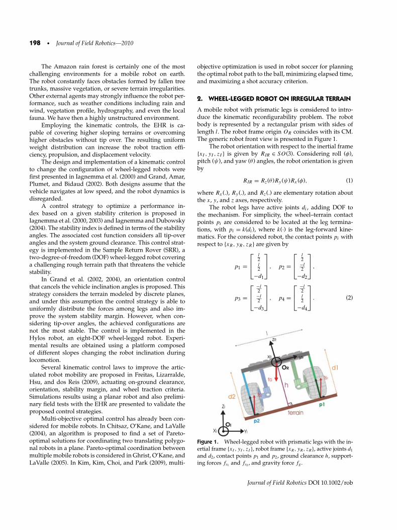
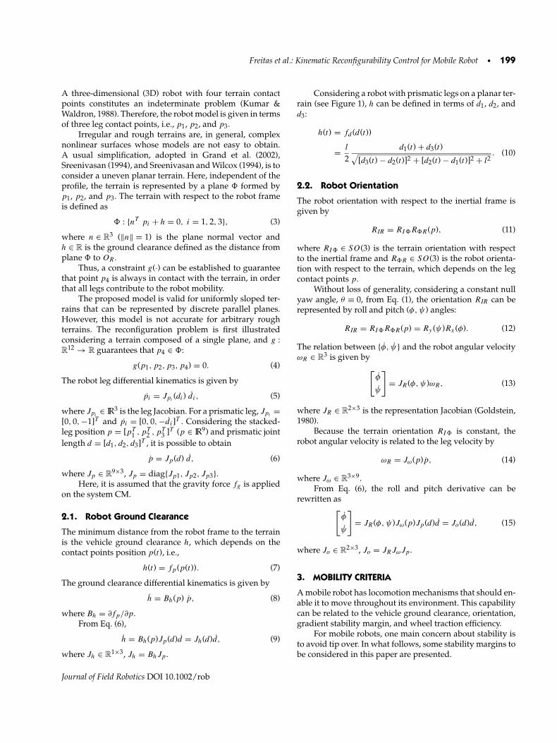
A mobile robot with prismatic legs is considered to intro-duce the kinematic reconfigurability problem. The robotbody is represented by a rectangular prism with sides oflength l. The robot frame origin OR coincides with its CM.The generic robot front view is presented in Figure 1.

The robot orientation with respect to the inertial frame{xI , yI , zI } is given by RIR ∈ SO(3). Considering roll (φ),pitch (ψ), and yaw (θ ) angles, the robot orientation is givenby

RIR = Rz(θ )Ry (ψ)Rx (φ), (1)

where Rx (.), Ry (.), and Rz(.) are elementary rotation aboutthe x, y, and z axes, respectively.

The robot legs have active joints di , adding DOF tothe mechanism. For simplicity, the wheel–terrain contactpoints pi are considered to be located at the leg termina-tions, with pi = k(di ), where k(·) is the leg-forward kine-matics. For the considered robot, the contact points pi withrespect to {xR, yR, zR} are given by

p1 =

⎡⎢⎣l2l2

−d1

⎤⎥⎦ , p2 =

⎡⎢⎣l2−l2

−d2

⎤⎥⎦ ,

p3 =

⎡⎢⎣−l2−l2

−d3

⎤⎥⎦ , p4 =

⎡⎢⎣−l2l2

−d4

⎤⎥⎦ . (2)

Figure 1. Wheel-legged robot with prismatic legs with the in-ertial frame {xI , yI , zI }, robot frame {xR, yR, zR}, active joints d1

and d2, contact points p1 and p2, ground clearance h, support-ing forces fs1 and fs2 , and gravity force fg .

Journal of Field Robotics DOI 10.1002/rob

Freitas et al.: Kinematic Reconfigurability Control for Mobile Robot • 199

A three-dimensional (3D) robot with four terrain contactpoints constitutes an indeterminate problem (Kumar &Waldron, 1988). Therefore, the robot model is given in termsof three leg contact points, i.e., p1, p2, and p3.

Irregular and rough terrains are, in general, complexnonlinear surfaces whose models are not easy to obtain.A usual simplification, adopted in Grand et al. (2002),Sreenivasan (1994), and Sreenivasan and Wilcox (1994), is toconsider a uneven planar terrain. Here, independent of theprofile, the terrain is represented by a plane � formed byp1, p2, and p3. The terrain with respect to the robot frameis defined as

� : {nT pi + h = 0, i = 1, 2, 3}, (3)

where n ∈ R3 (‖n‖ = 1) is the plane normal vector and

h ∈ R is the ground clearance defined as the distance fromplane � to OR .

Thus, a constraint g(·) can be established to guaranteethat point p4 is always in contact with the terrain, in orderthat all legs contribute to the robot mobility.

The proposed model is valid for uniformly sloped ter-rains that can be represented by discrete parallel planes.However, this model is not accurate for arbitrary roughterrains. The reconfiguration problem is first illustratedconsidering a terrain composed of a single plane, and g :R

12 → R guarantees that p4 ∈ �:

g(p1, p2, p3, p4) = 0. (4)

The robot leg differential kinematics is given by

pi = Jpi(di ) d i , (5)

where Jpi∈ IR3 is the leg Jacobian. For a prismatic leg, Jpi

=[0, 0, −1]T and pi = [0, 0, −d i ]T . Considering the stacked-leg position p = [pT

1 , pT2 , pT

3 ]T (p ∈ IR9) and prismatic jointlength d = [d1, d2, d3]T , it is possible to obtain

p = Jp(d) d, (6)

where Jp ∈ R9×3, Jp = diag{Jp1, Jp2, Jp3}.

Here, it is assumed that the gravity force fg is appliedon the system CM.

2.1. Robot Ground Clearance

The minimum distance from the robot frame to the terrainis the vehicle ground clearance h, which depends on thecontact points position p(t), i.e.,

h(t) = fp(p(t)). (7)

The ground clearance differential kinematics is given by

h = Bh(p) p, (8)

where Bh = ∂fp/∂p.From Eq. (6),

h = Bh(p)Jp(d)d = Jh(d)d, (9)

where Jh ∈ R1×3, Jh = BhJp .

Considering a robot with prismatic legs on a planar ter-rain (see Figure 1), h can be defined in terms of d1, d2, andd3:

h(t) = fd (d(t))

= l

2d1(t) + d3(t)√

[d3(t) − d2(t)]2 + [d2(t) − d1(t)]2 + l2. (10)

2.2. Robot Orientation

The robot orientation with respect to the inertial frame isgiven by

RIR = RI�R�R(p), (11)

where RI� ∈ SO(3) is the terrain orientation with respectto the inertial frame and R�R ∈ SO(3) is the robot orienta-tion with respect to the terrain, which depends on the legcontact points p.

Without loss of generality, considering a constant nullyaw angle, θ ≡ 0, from Eq. (1), the orientation RIR can berepresented by roll and pitch (φ,ψ) angles:

RIR = RI�R�R(p) = Ry (ψ)Rx (φ). (12)

The relation between {φ, ψ} and the robot angular velocityωR ∈ R

3 is given by[φ

ψ

]= JR(φ,ψ)ωR, (13)

where JR ∈ R2×3 is the representation Jacobian (Goldstein,

1980).Because the terrain orientation RI� is constant, the

robot angular velocity is related to the leg velocity by

ωR = Jω(p)p, (14)

where Jω ∈ R3×9.

From Eq. (6), the roll and pitch derivative can berewritten as[

φ

ψ

]= JR(φ,ψ)Jω(p)Jp(d)d = Jo(d)d, (15)

where Jo ∈ R2×3, Jo = JRJωJp .

3. MOBILITY CRITERIA

A mobile robot has locomotion mechanisms that should en-able it to move throughout its environment. This capabilitycan be related to the vehicle ground clearance, orientation,gradient stability margin, and wheel traction efficiency.

For mobile robots, one main concern about stability isto avoid tip over. In what follows, some stability margins tobe considered in this paper are presented.



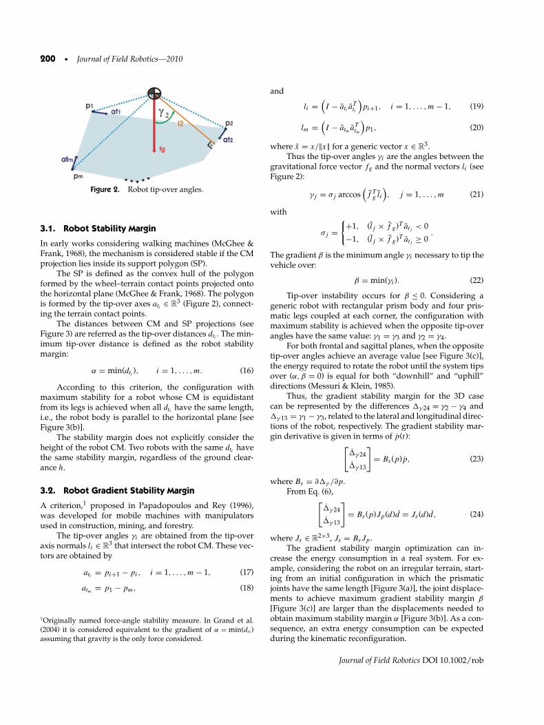
Figure 2. Robot tip-over angles.

3.1. Robot Stability Margin

In early works considering walking machines (McGhee &Frank, 1968), the mechanism is considered stable if the CMprojection lies inside its support polygon (SP).

The SP is defined as the convex hull of the polygonformed by the wheel–terrain contact points projected ontothe horizontal plane (McGhee & Frank, 1968). The polygonis formed by the tip-over axes ati ∈ R

3 (Figure 2), connect-ing the terrain contact points.

The distances between CM and SP projections (seeFigure 3) are referred as the tip-over distances dti . The min-imum tip-over distance is defined as the robot stabilitymargin:

α = min(dti ), i = 1, . . . , m. (16)

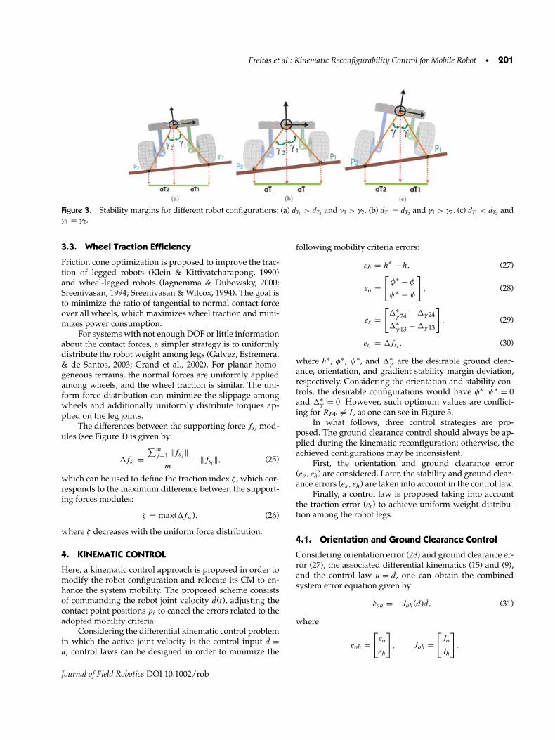
According to this criterion, the configuration withmaximum stability for a robot whose CM is equidistantfrom its legs is achieved when all dti have the same length,i.e., the robot body is parallel to the horizontal plane [seeFigure 3(b)].

The stability margin does not explicitly consider theheight of the robot CM. Two robots with the same dti havethe same stability margin, regardless of the ground clear-ance h.

3.2. Robot Gradient Stability Margin

A criterion,1 proposed in Papadopoulos and Rey (1996),was developed for mobile machines with manipulatorsused in construction, mining, and forestry.

The tip-over angles γi are obtained from the tip-overaxis normals li ∈ R

3 that intersect the robot CM. These vec-tors are obtained by

ati = pi+1 − pi, i = 1, . . . , m − 1, (17)

atm = p1 − pm, (18)

1Originally named force-angle stability measure. In Grand et al.(2004) it is considered equivalent to the gradient of α = min(dti)assuming that gravity is the only force considered.

and

li =(I − ati a

Tti

)pi+1, i = 1, . . . , m − 1, (19)

lm =(I − atm aT

tm

)p1, (20)

where x = x/||x|| for a generic vector x ∈ R3.

Thus the tip-over angles γi are the angles between thegravitational force vector fg and the normal vectors li (seeFigure 2):

γj = σj arccos(f T

g li

), j = 1, . . . , m (21)

with

σj ={

+1, (lj × f g)T atj < 0

−1, (lj × f g)T atj ≥ 0.

The gradient β is the minimum angle γi necessary to tip thevehicle over:

β = min(γi ). (22)

Tip-over instability occurs for β ≤ 0. Considering ageneric robot with rectangular prism body and four pris-matic legs coupled at each corner, the configuration withmaximum stability is achieved when the opposite tip-overangles have the same value: γ1 = γ3 and γ2 = γ4.

For both frontal and sagittal planes, when the oppositetip-over angles achieve an average value [see Figure 3(c)],the energy required to rotate the robot until the system tipsover (α, β = 0) is equal for both “downhill” and “uphill”directions (Messuri & Klein, 1985).

Thus, the gradient stability margin for the 3D casecan be represented by the differences �γ 24 = γ2 − γ4 and�γ 13 = γ1 − γ3, related to the lateral and longitudinal direc-tions of the robot, respectively. The gradient stability mar-gin derivative is given in terms of p(t):[

�γ 24

�γ 13

]= Bs (p)p, (23)

where Bs = ∂�γ /∂p.From Eq. (6),[

�γ 24

�γ 13

]= Bs (p)Jp(d)d = Js (d)d, (24)

where Js ∈ R2×3, Js = BsJp .

The gradient stability margin optimization can in-crease the energy consumption in a real system. For ex-ample, considering the robot on an irregular terrain, start-ing from an initial configuration in which the prismaticjoints have the same length [Figure 3(a)], the joint displace-ments to achieve maximum gradient stability margin β

[Figure 3(c)] are larger than the displacements needed toobtain maximum stability margin α [Figure 3(b)]. As a con-sequence, an extra energy consumption can be expectedduring the kinematic reconfiguration.



Figure 3. Stability margins for different robot configurations: (a) dT1 > dT2 and γ1 > γ2. (b) dT1 = dT2 and γ1 > γ2. (c) dT1 < dT2 andγ1 = γ2.

3.3. Wheel Traction Efficiency

Friction cone optimization is proposed to improve the trac-tion of legged robots (Klein & Kittivatcharapong, 1990)and wheel-legged robots (Iagnemma & Dubowsky, 2000;Sreenivasan, 1994; Sreenivasan & Wilcox, 1994). The goal isto minimize the ratio of tangential to normal contact forceover all wheels, which maximizes wheel traction and mini-mizes power consumption.

For systems with not enough DOF or little informationabout the contact forces, a simpler strategy is to uniformlydistribute the robot weight among legs (Galvez, Estremera,& de Santos, 2003; Grand et al., 2002). For planar homo-geneous terrains, the normal forces are uniformly appliedamong wheels, and the wheel traction is similar. The uni-form force distribution can minimize the slippage amongwheels and additionally uniformly distribute torques ap-plied on the leg joints.

The differences between the supporting force fsimod-

ules (see Figure 1) is given by

�fsi=

∑mj=1 ‖fsj

‖m

− ‖fsi‖, (25)

which can be used to define the traction index ζ , which cor-responds to the maximum difference between the support-ing forces modules:

ζ = max(�fsi), (26)

where ζ decreases with the uniform force distribution.

4. KINEMATIC CONTROL

Here, a kinematic control approach is proposed in order tomodify the robot configuration and relocate its CM to en-hance the system mobility. The proposed scheme consistsof commanding the robot joint velocity d(t), adjusting thecontact point positions pi to cancel the errors related to theadopted mobility criteria.

Considering the differential kinematic control problemin which the active joint velocity is the control input d =u, control laws can be designed in order to minimize the

following mobility criteria errors:

eh = h∗ − h, (27)

eo =[

φ∗ − φ

ψ∗ − ψ

], (28)

es =[�∗

γ 24 − �γ 24

�∗γ 13 − �γ 13

], (29)

eti = �fsi, (30)

where h∗, φ∗, ψ∗, and �∗γ are the desirable ground clear-

ance, orientation, and gradient stability margin deviation,respectively. Considering the orientation and stability con-trols, the desirable configurations would have φ∗, ψ∗ = 0and �∗

γ = 0. However, such optimum values are conflict-ing for RI� = I , as one can see in Figure 3.

In what follows, three control strategies are pro-posed. The ground clearance control should always be ap-plied during the kinematic reconfiguration; otherwise, theachieved configurations may be inconsistent.

First, the orientation and ground clearance error(eo, eh) are considered. Later, the stability and ground clear-ance errors (es, eh) are taken into account in the control law.

Finally, a control law is proposed taking into accountthe traction error (et ) to achieve uniform weight distribu-tion among the robot legs.

4.1. Orientation and Ground Clearance Control

Considering orientation error (28) and ground clearance er-ror (27), the associated differential kinematics (15) and (9),and the control law u = d , one can obtain the combinedsystem error equation given by

eoh = −Joh(d)d, (31)

where

eoh =[eo

eh

], Joh =

[Jo

Jh

].



Assuming that Joh is nonsingular for di > 0, the control lawis given by

u = J−1oh (d)Koh eoh, Koh > 0, (32)

where Koh ∈ IR3×3 is the controller gain.Thus, the stable closed-loop system error equation is

given by

eoh = −Koh eoh. (33)

Then, the error eoh tends to zero as t → ∞.

Remark 1. The joint velocity d4 can be obtained, in termsof d , differentiating constraint (4):

d4 = −[

dg

dp4Jp4 (d4)

]−1dg

dpJp(d) d, (34)

where ( dgdp4

Jp4 ) is assumed to be nonsingular.

4.2. Stability and Ground Clearance Control

Considering the stability error (29) and ground clearanceerror (27), the associated differential kinematics (24) and (9),and control law u = d , one can obtain the combined systemerror equation given by

esh = −Jsh(d) d, (35)

where

esh =[es

eh

], Jsh =

[Js

Jh

].

Assuming that Jsh is nonsingular for di > 0, the control lawis given by

u = J−1sh Ksh esh, Ksh > 0, (36)

where Ksh ∈ IR3×3 is the controller gain.Thus, the stable closed-loop system error equation is

given by

esh = −Ksh esh. (37)

Then, the error esh tends to zero as t → ∞.

4.3. Traction Control

A traction control can be designed to uniformly distributethe load forces among all wheels, canceling the traction er-ror (30).

For a 3D robot with four legs, the relation betweenp and et is not easily obtained. On almost-horizontal ter-rains, it is possible to observe that the supported force fsi

increases with the vertical component of the contact pointpi enlargement.

Therefore, considering ui = d i , the following propor-tional control law can be proposed:

ui = (ez Jpi)−1 kti eti , kti > 0, (38)

where kti ∈ IR is the controller gain, ez = [0, 0, 1], andezJpi

= 0.

4.4. Multi-Objective Optimization

The mobility criteria for orientation and stability presentedin Section 3 cannot both be canceled for RI� = I, h > 0.In fact, they are conflicting objectives; thus when one at-tempts to achieve an optimal configuration that cancels oneof them, it leads to a worse result in the other criterion.

An optimization problem that involves conflicting ob-jectives is called the multi-objective optimization problem(MOOP), which can be written in the form

minimize f1(x), f2(x), . . . , fm(x),

subject to x ∈ S,(39)

with m(≥2) objective functions fi : IRn → IRm.In MOOPs, the objective functions constitute a multi-

dimensional space, in addition to the decision variablespace (or search space). This additional space is called ob-jective space Z . For each decision vector x ∈ R

n in thesearch space S, there exists a point in the objective space,denoted by z = f (x), z ∈ IRm.

The main difference between single- and multi-objective optimization problems is that the latter does nothave a unique optimal solution. For instance, there is aset of solutions that can be called optimal, because multi-objective optimization does not consider any relative im-portance between the objectives. The set of optimal solu-tions is called a Pareto-optimal set. A Pareto-optimal solutionis defined as follows:

Definition 1. A decision vector x∗ ∈ S is a Pareto-optimalsolution if there is no other decision vector x ∈ S such thatfi (x) ≤ fi (x∗) for all i = 1, . . . , m and fj (x) < fj (x∗) for atleast one index j .

This definition means that a Pareto-optimal solution isbetter than any other in at least one objective.

Even though there is a set of optimal solutions for aMOOP, for a given problem only one solution is needed.Two approaches are used to find a solution.

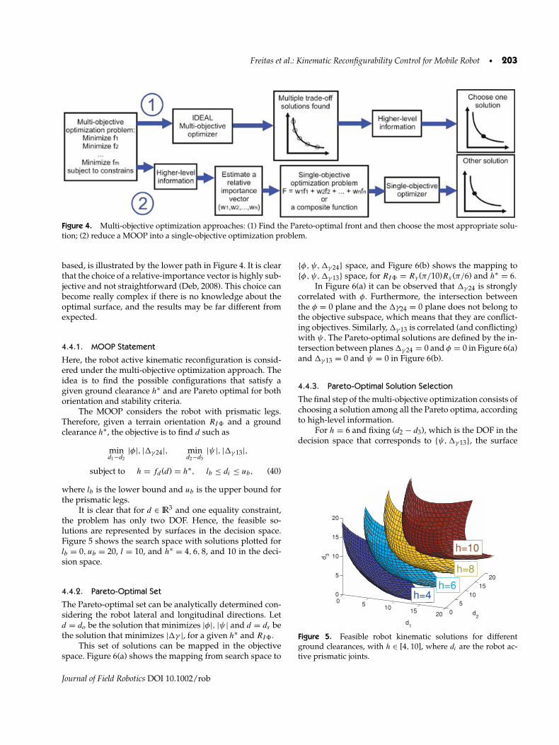
A more appropriate approach is to find the Pareto-optimal front or a set of solutions in it, which should be welldistributed along the front. Then, by using high-level infor-mation, a decision-making algorithm can choose which ofthem is the most appropriate. This approach is illustratedby the upper path in Figure 4.

Another approach could be defined as transforming aMOOP into a single-objective optimization problem. Thiscan be done by estimating a relative importance vectorbetween the objectives and making a composite function,such as a weighted sum of the objectives. Afterward, anysingle-objective optimization technique may be used to getto an optimal solution. This approach, called preference



Figure 4. Multi-objective optimization approaches: (1) Find the Pareto-optimal front and then choose the most appropriate solu-tion; (2) reduce a MOOP into a single-objective optimization problem.

based, is illustrated by the lower path in Figure 4. It is clearthat the choice of a relative-importance vector is highly sub-jective and not straightforward (Deb, 2008). This choice canbecome really complex if there is no knowledge about theoptimal surface, and the results may be far different fromexpected.

4.4.1. MOOP Statement

Here, the robot active kinematic reconfiguration is consid-ered under the multi-objective optimization approach. Theidea is to find the possible configurations that satisfy agiven ground clearance h∗ and are Pareto optimal for bothorientation and stability criteria.

The MOOP considers the robot with prismatic legs.Therefore, given a terrain orientation RI� and a groundclearance h∗, the objective is to find d such as

mind1−d2

|φ|, |�γ 24|, mind2−d3

|ψ |, |�γ 13|,

subject to h = fd (d) = h∗, lb ≤ di ≤ ub, (40)

where lb is the lower bound and ub is the upper bound forthe prismatic legs.

It is clear that for d ∈ IR3 and one equality constraint,the problem has only two DOF. Hence, the feasible so-lutions are represented by surfaces in the decision space.Figure 5 shows the search space with solutions plotted forlb = 0, ub = 20, l = 10, and h∗ = 4, 6, 8, and 10 in the deci-sion space.

4.4.2. Pareto-Optimal Set

The Pareto-optimal set can be analytically determined con-sidering the robot lateral and longitudinal directions. Letd = do be the solution that minimizes |φ|, |ψ | and d = ds bethe solution that minimizes |�γ |, for a given h∗ and RI�.

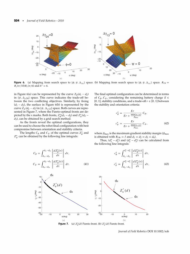
This set of solutions can be mapped in the objectivespace. Figure 6(a) shows the mapping from search space to

{φ,ψ, �γ 24} space, and Figure 6(b) shows the mapping to{φ,ψ, �γ 13} space, for RI� = Ry (π/10)Rx (π/6) and h∗ = 6.

In Figure 6(a) it can be observed that �γ 24 is stronglycorrelated with φ. Furthermore, the intersection betweenthe φ = 0 plane and the �γ24 = 0 plane does not belong tothe objective subspace, which means that they are conflict-ing objectives. Similarly, �γ 13 is correlated (and conflicting)with ψ . The Pareto-optimal solutions are defined by the in-tersection between planes �γ 24 = 0 and φ = 0 in Figure 6(a)and �γ 13 = 0 and ψ = 0 in Figure 6(b).

4.4.3. Pareto-Optimal Solution Selection

The final step of the multi-objective optimization consists ofchoosing a solution among all the Pareto optima, accordingto high-level information.

For h = 6 and fixing (d2 − d3), which is the DOF in thedecision space that corresponds to {ψ, �γ 13}, the surface

05

1015

20 0

5

10

15

20

0

5

10

15

20

d2

d1

d3

h=4h=6

h=10

h=8

Figure 5. Feasible robot kinematic solutions for differentground clearances, with h ∈ [4, 10], where di are the robot ac-tive prismatic joints.



10 0 10 20 30

20

0

2030

20

10

0

10

20

φ (deg)ψ (deg)

Δγ24 (

deg)

φ=0

Δγ24

=0

10

0

10

20

30 100

1020

20

10

0

10

ψ (deg)φ (deg)

Δγ13 (

deg)

ψ = 0

Δγ13

= 0

)b()a(

Figure 6. (a) Mapping from search space to {φ,ψ,�γ24 } space. (b) Mapping from search space to {φ,ψ,�γ13 } space. RI� =Ry (π/10)Rx (π/6) and h∗ = 6.

in Figure 6(a) can be represented by the curve Zφ(d1 − d2)in {ψ, �γ 24} space. This curve indicates the trade-off be-tween the two conflicting objectives. Similarly, by fixing(d1 − d2), the surface in Figure 6(b) is represented by thecurve Zψ (d2 − d3) in {ψ,�γ 13} space. Both curves are repre-sented in Figure 7, where the Pareto-optimal fronts are de-picted by the x marks. Both fronts, Z∗

φ(d1 − d2) and Z∗ψ (d2 −

d3), can be obtained by a grid search method.As the fronts reveal the optimal configurations, they

can be used to choose the robot final configuration with bestcompromise between orientation and stability criteria.

The lengths Cφ and Cψ of the optimal curves Z∗φ and

Z∗ψ can be obtained by the following line integrals:

Cφ =∫ d1s−d2s

d1o−d2o

∣∣∣∣∣∣∣∣∣∣dZ∗

φ(τ )

dτ

∣∣∣∣∣∣∣∣∣∣ dτ,

Cψ =∫ d2s−d3s

d2o−d3o

∣∣∣∣∣∣∣∣∣∣dZ∗

ψ (τ )

dτ

∣∣∣∣∣∣∣∣∣∣ dτ. (41)

The final optimal configuration can be determined in termsof Cφ,Cψ , considering the remaining battery charge E ∈[0, 1], stability conditions, and a trade-off r ∈ [0, 1] betweenthe stability and orientation criteria:

c∗φ = Er

Er + min(γ2,γ4)βmax

Cφ,

c∗ψ = Er

Er + min(γ1,γ3)βmax

Cψ, (42)

where βmax is the maximum gradient stability margin (βmaxis obtained with RI� = I and d1 = d2 = d3 = d4).

Thus, (d∗1 − d∗

2 ) and (d∗2 − d∗

3 ) can be calculated fromthe following line integrals:

c∗φ =

∫ d∗1 −d∗

2

d1o −d2o

∣∣∣∣∣∣∣∣∣∣dZ∗

φ(τ )

dτ

∣∣∣∣∣∣∣∣∣∣ dτ,

c∗ψ =

∫ d∗2 −d∗

3

d2o −d3o

∣∣∣∣∣∣∣∣∣∣dZ∗

ψ (τ )

dτ

∣∣∣∣∣∣∣∣∣∣ dτ, (43)

(a) (b)

Figure 7. (a) Z∗φ(d) Pareto front. (b) Z∗

ψ (d) Pareto front.



where c∗φ and c∗

ψ are given by Eqs. (42). The integral upperlimits can be calculated through the accumulation numeri-cal method.

Considering constant h, is is possible to obtain (d∗1 +

d∗3 ). The robot optimal configuration d∗ = [d∗

1 , d∗2 , d∗

3 ]T canbe obtained from (d∗

1 − d∗2 ), (d∗

2 − d∗3 ), and (d∗

1 + d∗3 ).

Then, from the robot forward kinematics, h∗, φ∗, ψ∗can be obtained in terms of d∗ and then employed as ref-erence in the orientation control (32).

5. SIMULATION RESULTS

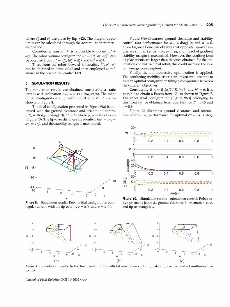
The simulation results are obtained considering a staticterrain with inclination RI� = Ry (π/10)Rx (π/6). The robotinitial configuration (IC) with l = 10 and ∀i : di = 6 isshown in Figure 8.

The final configuration presented in Figure 9(a) is ob-tained with the ground clearance and orientation control(32), with Koh = diag{10}, h∗ = 6, where φ,ψ → 0 as t → ∞(Figure 10). The tip-over distances are identical (dT1 = dT2 =dT3 = dT4 ), and the stability margin is maximized.

Figure 8. Simulation results: Robot initial configuration on ir-regular terrain, with the tip-over γi , φ = π/6, and ψ = π/10.

Figure 9(b) illustrates ground clearance and stabilitycontrol (36) performance for Ksh = diag{10} and h∗ = 6.From Figure 11 one can observe that opposite tip-over an-gles are similar, i.e., γ1 = γ3, γ2 = γ4, and the robot gradientstability margin is maximized. However, the resulting jointdisplacements are larger than the ones obtained for the ori-entation control. In a real robot, this could increase the sys-tem energy consumption.

Finally, the multi-objective optimization is applied.The conflicting mobility criteria are taken into account tofind an optimal configuration filling a compromise betweenthe different objectives.

Considering RI� = Ry (π/10)Rx (π/6) and h∗ = 6, it ispossible to obtain a Pareto front Z∗, as shown in Figure 7.The robot final configuration [Figure 9(c)] belonging tothis front can be obtained from Eqs. (42), for E = 0.65 andr = 0.9.

Figure 12 illustrates ground clearance and orienta-tion control (32) performance for optimal φ∗ = −6.30 deg,

0 0.2 0.4 0.6 0.8 10

10

20d

i

0 0.2 0.4 0.6 0.8 15

6

7

h

0 0.2 0.4 0.6 0.8 10

20

40

φ,ψ

(deg)

0 0.2 0.4 0.6 0.8 10

50

100

γ i (deg)

time(s)

Figure 10. Simulation results—orientation control: Robot ac-tive prismatic joints di , ground clearance h, orientation φ,ψ ,and tip-over angles γi .

10

0

10

105051015

10

5

0

5

XiYi

Zi

10

0

10

105051015

10

5

0

5

XiYi

Zi

10

0

10

105051015

10

5

0

5

XiYi

Zi

(c)(b)(a)

Figure 9. Simulation results: Robot final configuration with (a) orientation control (b) stability control, and (c) multi-objectivecontrol.



0 0.2 0.4 0.6 0.8 10

10

20

di

0 0.2 0.4 0.6 0.8 15

6

7

h

0 0.2 0.4 0.6 0.8 150

0

50

φ,ψ

(deg)

0 0.2 0.4 0.6 0.8 10

50

100

γ i (deg)

time(s)

Figure 11. Simulations results—stability control: Robot activeprismatic joints di , ground clearance h, orientation φ,ψ , andtip-over angles γi .

ψ∗ = −2.18 deg, and Koh = diag{10}. The final achievedconfiguration fills an optimal trade-off between the orien-tation and gradient stability margin conflicting criteria.

Table I compares simulation results obtained with allproposed controllers.

6. ENVIRONMENTAL HYBRID ROBOT

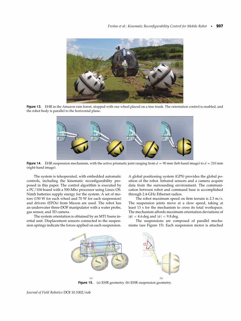
The proposed strategies are experimentally tested using theEHR from Petrobras S.A. (Figure 13). The robot, being usedas a maintenance tool for the Coari–Manaus pipeline, is go-ing to help in monitoring the Amazon rain forest region.

An innovative locomotion system is controlled accord-ing to the conditions encountered in the Amazon. Thewheel-legged architecture is adopted, allowing the robot to

0 0.2 0.4 0.6 0.8 10

10

20

di

0 0.2 0.4 0.6 0.8 15

6

7

h

0 0.2 0.4 0.6 0.8 150

0

50

φ,ψ

(deg)

0 0.2 0.4 0.6 0.8 10

50

100

γ i (deg)

time(s)

Figure 12. Simulations results—multi-objective control:Robot active prismatic joints di , ground clearance h, orienta-tion φ,ψ , and tip-over angles γi .

carry load, save energy, and be able to work on irregularterrains.

The robot uses four wheels to move. Aiming to enableit to float in the water, the wheels have a large volume andare made of low-density material. Each wheel is coupledto an independent suspension system, also referred to aslegs in this paper, composed of spring and electric actuator,with one DOF. Commanding this mechanism, it is possibleto change the wheel configuration, as shown in Figure 14.More details related to the leg mechanisms can be found indos Reis (2007a, 2007b).

The mobile robot weighs 150 kg and has a wheelbaseof 730 mm, track width ∼1,350 mm, and minimum groundclearance h∗ = 680 mm.

Table I. Simulations with the initial and steady-state values obtained with the wheel-legged robot with prismatic legs employingthe different proposed controllers.

Multi-objectiveInitial conditions Orientation control control Stability control

Joint length d1 6 5.93 5.92 6.15d2 6 11.71 13.27 16.53d3 6 8.46 9.59 11.99d4 6 2.68 2.24 1.60

Ground clearance h 6 6 6 6Robot orientation RI� φ (deg) 30 0 −6.30 −16.07

ψ (deg) 18 0 −2.18 −6.43Tip-over angles γ1 (deg) 36.48 43.56 45.08 47.96

γ2 (deg) 17.66 32.50 35.86 41.2γ3 (deg) 62.52 53.04 51.34 47.96γ4 (deg) 71.78 52.93 48.55 41.3

Gradient stability margin β 17.66 32.50 35.86 41.2Stability increment w.r.t. βIC 84% 103% 133%



Figure 13. EHR in the Amazon rain forest, stopped with one wheel placed on a tree trunk. The orientation control is enabled, andthe robot body is parallel to the horizontal plane.

Figure 14. EHR suspension mechanism, with the active prismatic joint ranging from d = 90 mm (left-hand image) to d = 210 mm(right-hand image).

The system is teleoperated, with embedded automaticcontrols, including the kinematic reconfigurability pro-posed in this paper. The control algorithm is executed bya PC/104 board with a 500-Mhz processor using Linux OS.Nimh batteries supply energy for the system. A set of mo-tors (150 W for each wheel and 70 W for each suspension)and drivers (EPOs) from Maxon are used. The robot hasan underwater three-DOF manipulator with a water probe,gas sensor, and 3D camera.

The system orientation is obtained by an MTI Xsens in-ertial unit. Displacement sensors connected to the suspen-sion springs indicate the forces applied on each suspension.

A global positioning system (GPS) provides the global po-sition of the robot. Infrared sensors and a camera acquiredata from the surrounding environment. The communi-cation between robot and command base is accomplishedthrough 2.4-GHz Ethernet radios.

The robot maximum speed on firm terrain is 2.3 m/s.The suspension joints move at a slow speed, taking atleast 13 s for the mechanism to cross its total workspace.The mechanism affords maximum orientation deviations of|φ| < 4.6 deg and |ψ | < 9.8 deg.

The suspensions are composed of parallel mecha-nisms (see Figure 15). Each suspension motor is attached

Figure 15. (a) EHR geometry. (b) EHR suspension geometry.



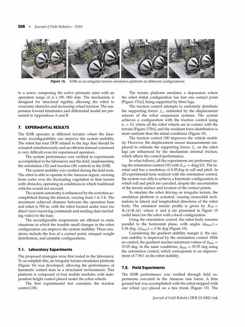
Figure 16. EHR on an irregular terrain emulation platform in different configurations.

to a screw, composing the active prismatic joint with anoperation range of di ∈ (90, 180) mm. The mechanism isdesigned for structural rigidity, allowing the robot toovercome obstacles and increasing wheel traction. The sus-pension foward kinematics and differential model are pre-sented in Appendixes A and B.

7. EXPERIMENTAL RESULTS

The EHR operates in different terrains where the kine-matic reconfigurability can improve the system mobility.The robot has four DOF related to the legs that should beactuated simultaneously, and an efficient manual commandis very difficult even for experienced operators.

The system performance was verified in experimentsaccomplished in the laboratory and the field, implementingthe orientation (32) and traction (38) controls in the EHR.

The system mobility was verified during the field tests.The robot is able to operate in the Amazon region, crossingfrom water over the fluctuating vegetation to firm terrainwith obstacles, operating in conditions in which traditionalvehicles would not succeed.

The system autonomy is influenced by the activities ac-complished during the mission, varying from 1 to 3 h. Themaximum achieved distance between the operation baseand robot is 700 m, with the robot located under trees (nodirect view) receiving commands and sending data (includ-ing video) to the base.

The reconfigurable suspensions are efficient in staticsituations in which the feasible small changes in the robotconfiguration can improve the system mobility. These situ-ations include the loss of a contact point, unequal weightdistribution, and unstable configurations.

7.1. Laboratory Experiments

The proposed strategies were first tested in the laboratory.To accomplish this, an irregular terrain emulation platform(Figure 16) was developed, allowing the performance ofkinematic control tests in a structured environment. Thisplatform is composed of four mobile modules with inde-pendent height control placed under the robot wheels.

The first experimental test considers the tractioncontrol (38).

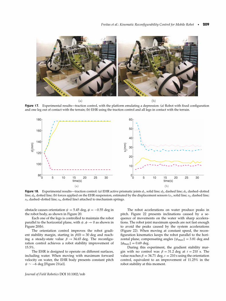
The terrain platform emulates a depression wherethe robot initial configuration has lost one contact point[Figure 17(a)], being supported by three legs.

The traction control attempts to uniformly distributethe supporting forces fsi

, estimated by the displacementsensors of the robot suspension systems. The systemachieves a configuration with the traction control usingkt = 10, where all the robot wheels are in contact with theterrain [Figure 17(b)], and the resultant force distribution ismore uniform than the initial conditions (Figure 18).

The traction control (38) improves the vehicle mobil-ity. However, the displacement sensor measurements em-ployed to estimate the supporting forces fsi

on the robotlegs are influenced by the mechanism internal friction,which affects the control performance.

In what follows, all the experiments are performed us-ing the orientation control (32) with Koh = diag{10}. The in-ertial unit has a resolution of 0.05 deg in roll and pitch. Inall experimental tests realized with the orientation control,the system was able to achieve a kinematic configuration inwhich roll and pitch are canceled, despite the uncertaintiesof the terrain surface and location of the contact points.

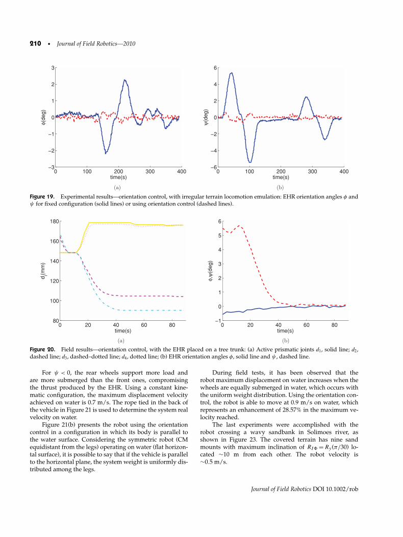
To emulate the robot driving on irregular terrain, theemulation platform is actuated, causing sinusoidal incli-nations in lateral and longitudinal directions of the robotbody. The emulated terrain profile is given by RI� =Ry (ψ)Rx (φ), where ψ and φ are presented in Figure 19(solid lines) for the robot with a fixed configuration.

Using the orientation control, the robot body remainsparallel to the horizontal plane, with angles ‖φmax‖ =0.38 deg, ‖ψmax‖ = 0.56 deg (Figure 19).

Considering the gradient stability margin β, the sys-tem stability is improved by the orientation control. Withno control, the gradient reaches minimum values of βmin =33.05 deg. In the same conditions, βmin = 35.55 deg usingthe orientation control, which corresponds to an improve-ment of 7.56% in the robot stability.

7.2. Field Experiments

The EHR performance was verified through field ex-periments executed in the Amazon rain forest. A firmground test was accomplished with the robot stopped withone wheel (p3) placed on a tree trunk (Figure 13). The



Figure 17. Experimental results—traction control, with the platform emulating a depression: (a) Robot with fixed configurationand one leg out of contact with the terrain; (b) EHR using the traction control and all legs in contact with the terrain.

0 5 10 15 20 25 3080

100

120

140

160

180

time(s)

di(m

m)

0 5 10 15 20 25 300

10

20

30

40

50

60

time(s)

s i(mm

)

(a) (b)

Figure 18. Experimental results—traction control: (a) EHR active prismatic joints d1, solid line; d2, dashed line; d3, dashed–dottedline; d4, dotted line; (b) forces applied on the EHR suspension, estimated by the displacement sensors (s1, solid line; s2, dashed line;s3, dashed–dotted line; s4, dotted line) attached to mechanism springs.

obstacle causes orientation ψ = 5.45 deg, φ = −0.55 deg inthe robot body, as shown in Figure 20.

Each one of the legs is controlled to maintain the robotparallel to the horizontal plane, with ψ, φ → 0 as shown inFigure 20(b).

The orientation control improves the robot gradi-ent stability margin, starting in β(0) = 30 deg and reach-ing a steady-state value β → 34.65 deg. The reconfigu-ration control achieves a robot stability improvement of15.5%.

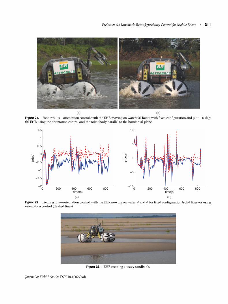
The EHR is designed to operate on different surfaces,including water. When moving with maximum forwardvelocity on water, the EHR body presents constant pitchψ ∼ −6 deg [Figure 21(a)].

The robot accelerations on water produce peaks inpitch. Figure 22 presents inclinations caused by a se-quence of movements on the water with sharp accelera-tions. The robot joint maximum speeds are not fast enoughto avoid the peaks caused by the system accelerations(Figure 22). When moving at constant speed, the recon-figuration kinematics keeps the robot parallel to the hori-zontal plane, compensating angles ‖ψmax‖ = 3.81 deg and‖φmax‖ = 0.69 deg.

During this experiment, the gradient stability mar-gin with no control was β = 31.2 deg at t = 210 s. Thevalue reaches β = 34.71 deg, t = 210 s using the orientationcontrol, equivalent to an improvement of 11.25% in therobot stability at this moment.



0 100 200 300 4003

2

1

0

1

2

3

time(s)

φ(d

eg

)

0 100 200 300 4006

4

2

0

2

4

6

time(s)

ψ(d

eg

)

)b()a(

Figure 19. Experimental results—orientation control, with irregular terrain locomotion emulation: EHR orientation angles φ andψ for fixed configuration (solid lines) or using orientation control (dashed lines).

0 20 40 60 8080

100

120

140

160

180

time(s)

di(m

m)

0 20 40 60 801

0

1

2

3

4

5

6

time(s)

φ,ψ

(de

g)

)b()a(

Figure 20. Field results—orientation control, with the EHR placed on a tree trunk: (a) Active prismatic joints d1, solid line; d2,dashed line; d3, dashed–dotted line; d4, dotted line; (b) EHR orientation angles φ, solid line and ψ , dashed line.

For ψ < 0, the rear wheels support more load andare more submerged than the front ones, compromisingthe thrust produced by the EHR. Using a constant kine-matic configuration, the maximum displacement velocityachieved on water is 0.7 m/s. The rope tied in the back ofthe vehicle in Figure 21 is used to determine the system realvelocity on water.

Figure 21(b) presents the robot using the orientationcontrol in a configuration in which its body is parallel tothe water surface. Considering the symmetric robot (CMequidistant from the legs) operating on water (flat horizon-tal surface), it is possible to say that if the vehicle is parallelto the horizontal plane, the system weight is uniformly dis-tributed among the legs.

During field tests, it has been observed that therobot maximum displacement on water increases when thewheels are equally submerged in water, which occurs withthe uniform weight distribution. Using the orientation con-trol, the robot is able to move at 0.9 m/s on water, whichrepresents an enhancement of 28.57% in the maximum ve-locity reached.

The last experiments were accomplished with therobot crossing a wavy sandbank in Solimoes river, asshown in Figure 23. The covered terrain has nine sandmounts with maximum inclination of RI� = Ry (π/30) lo-cated ∼10 m from each other. The robot velocity is∼0.5 m/s.



Figure 21. Field results—orientation control, with the EHR moving on water: (a) Robot with fixed configuration and ψ ∼ −6 deg;(b) EHR using the orientation control and the robot body parallel to the horizontal plane.

0 200 400 600 8002

1.5

1

0.5

0

0.5

1

1.5

time(s)

φ (d

eg

)

0 200 400 600 80010

5

0

5

10

time(s)

ψ(d

eg

)

)b()a(

Figure 22. Field results—orientation control, with the EHR moving on water: φ and ψ for fixed configuration (solid lines) or usingorientation control (dashed lines).

Figure 23. EHR crossing a wavy sandbank.



0 50 100 150 2004

2

0

2

4

6

time(s)

φ(d

eg

)

0 50 100 150 20010

8

6

4

2

0

2

4

6

time(s)

ψ(d

eg

)

)b()a(

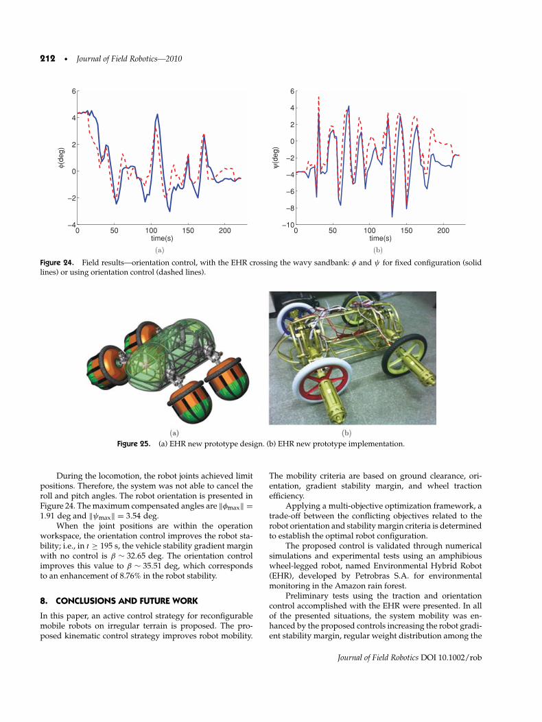
Figure 24. Field results—orientation control, with the EHR crossing the wavy sandbank: φ and ψ for fixed configuration (solidlines) or using orientation control (dashed lines).

Figure 25. (a) EHR new prototype design. (b) EHR new prototype implementation.

During the locomotion, the robot joints achieved limitpositions. Therefore, the system was not able to cancel theroll and pitch angles. The robot orientation is presented inFigure 24. The maximum compensated angles are ‖φmax‖ =1.91 deg and ‖ψmax‖ = 3.54 deg.

When the joint positions are within the operationworkspace, the orientation control improves the robot sta-bility; i.e., in t ≥ 195 s, the vehicle stability gradient marginwith no control is β ∼ 32.65 deg. The orientation controlimproves this value to β ∼ 35.51 deg, which correspondsto an enhancement of 8.76% in the robot stability.

8. CONCLUSIONS AND FUTURE WORK

In this paper, an active control strategy for reconfigurablemobile robots on irregular terrain is proposed. The pro-posed kinematic control strategy improves robot mobility.

The mobility criteria are based on ground clearance, ori-entation, gradient stability margin, and wheel tractionefficiency.

Applying a multi-objective optimization framework, atrade-off between the conflicting objectives related to therobot orientation and stability margin criteria is determinedto establish the optimal robot configuration.

The proposed control is validated through numericalsimulations and experimental tests using an amphibiouswheel-legged robot, named Environmental Hybrid Robot(EHR), developed by Petrobras S.A. for environmentalmonitoring in the Amazon rain forest.

Preliminary tests using the traction and orientationcontrol accomplished with the EHR were presented. In allof the presented situations, the system mobility was en-hanced by the proposed controls increasing the robot gradi-ent stability margin, regular weight distribution among the



legs, and hence wheel traction and displacement velocityon water.

When using a fixed kinematic configuration, the robotcan tip over when crossing terrains or obstacles withinclination larger than 35 deg. The kinematic reconfigura-tion increases this value up to 44.8 deg, which correspondsto an obstacle negotiation enhancement of 28%.

The control strategy performance depends on the qual-ity of the feedback data. Future works will consider moreprecise wheel–terrain contact point positions instead of us-ing ad hoc approximate values corresponding to the leg ter-minations. These positions could be calculated using tech-niques similar to the wheel–ground contact angle estima-tion proposed in Iagnemma and Dubowsky (2000). Theforces applied to the robot legs should be directly measuredby sensors placed on the robot legs in order to avoid inter-nal friction interference, which can affect the indirect mea-surements as done so far. The terrain should be consideredas nonplanar, and a realistic model should be acquired withappropriate sensors.

Considering low-speed navigation, a quasi-static ap-proach was adopted. However, for medium and high navi-gation speed, the system dynamics must be considered andthe mobility criteria adopted should be revised.

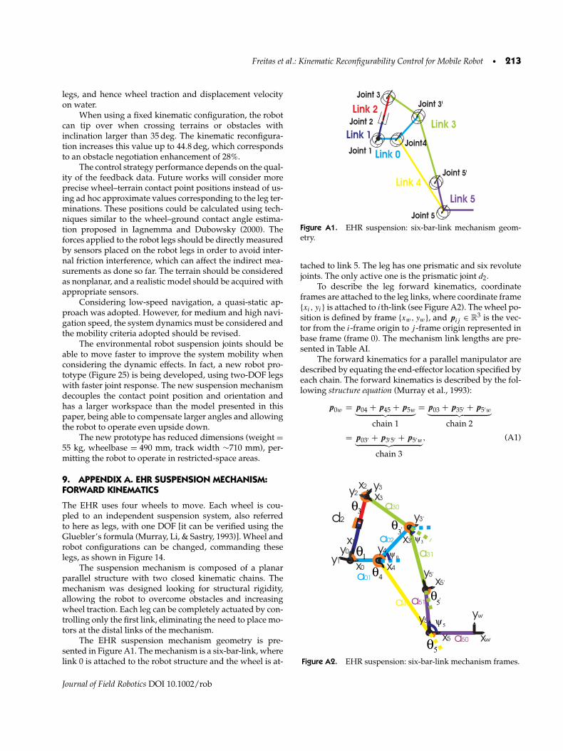
The environmental robot suspension joints should beable to move faster to improve the system mobility whenconsidering the dynamic effects. In fact, a new robot pro-totype (Figure 25) is being developed, using two-DOF legswith faster joint response. The new suspension mechanismdecouples the contact point position and orientation andhas a larger workspace than the model presented in thispaper, being able to compensate larger angles and allowingthe robot to operate even upside down.

The new prototype has reduced dimensions (weight =55 kg, wheelbase = 490 mm, track width ∼710 mm), per-mitting the robot to operate in restricted-space areas.

9. APPENDIX A. EHR SUSPENSION MECHANISM:FORWARD KINEMATICS

The EHR uses four wheels to move. Each wheel is cou-pled to an independent suspension system, also referredto here as legs, with one DOF [it can be verified using theGluebler’s formula (Murray, Li, & Sastry, 1993)]. Wheel androbot configurations can be changed, commanding theselegs, as shown in Figure 14.

The suspension mechanism is composed of a planarparallel structure with two closed kinematic chains. Themechanism was designed looking for structural rigidity,allowing the robot to overcome obstacles and increasingwheel traction. Each leg can be completely actuated by con-trolling only the first link, eliminating the need to place mo-tors at the distal links of the mechanism.

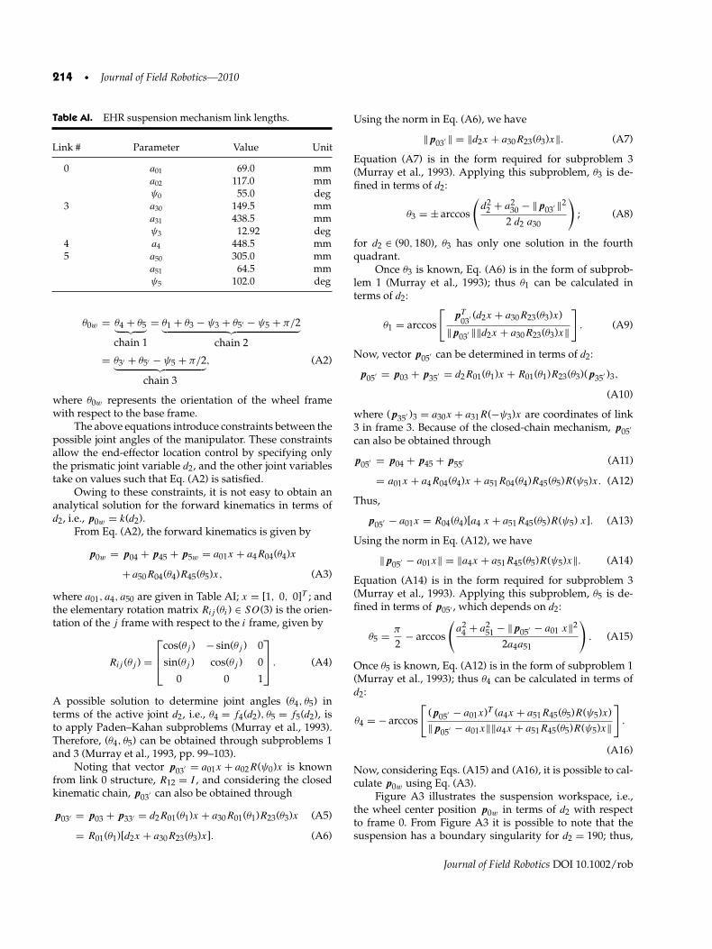
The EHR suspension mechanism geometry is pre-sented in Figure A1. The mechanism is a six-bar-link, wherelink 0 is attached to the robot structure and the wheel is at-

Figure A1. EHR suspension: six-bar-link mechanism geom-etry.

tached to link 5. The leg has one prismatic and six revolutejoints. The only active one is the prismatic joint d2.

To describe the leg forward kinematics, coordinateframes are attached to the leg links, where coordinate frame{xi, yi} is attached to ith-link (see Figure A2). The wheel po-sition is defined by frame {xw, yw}, and pij ∈ R

3 is the vec-tor from the i-frame origin to j -frame origin represented inbase frame (frame 0). The mechanism link lengths are pre-sented in Table AI.

The forward kinematics for a parallel manipulator aredescribed by equating the end-effector location specified byeach chain. The forward kinematics is described by the fol-lowing structure equation (Murray et al., 1993):

p0w = p04 + p45 + p5w︸︷︷︸chain 1

= p03 + p35′ + p5′w︸︷︷︸chain 2

= p03′ + p3′5′ + p5′w︸︷︷︸chain 3

, (A1)

1

3

4

5

'3

x1

y1

x5

y5

x2y2 x3

y3

xw

yw

x0

y0

x5'y5'

x4

y4

x3'

y3'

a50

a51

d2

a30

a31

a4

a01

a02

'5

3

5

0

Figure A2. EHR suspension: six-bar-link mechanism frames.



Table AI. EHR suspension mechanism link lengths.

Link # Parameter Value Unit

0 a01 69.0 mma02 117.0 mmψ0 55.0 deg

3 a30 149.5 mma31 438.5 mmψ3 12.92 deg

4 a4 448.5 mm5 a50 305.0 mm

a51 64.5 mmψ5 102.0 deg

θ0w = θ4 + θ5︸︷︷︸chain 1

= θ1 + θ3 − ψ3 + θ5′ − ψ5 + π/2︸︷︷︸chain 2

= θ3′ + θ5′ − ψ5 + π/2︸︷︷︸chain 3

, (A2)

where θ0w represents the orientation of the wheel framewith respect to the base frame.

The above equations introduce constraints between thepossible joint angles of the manipulator. These constraintsallow the end-effector location control by specifying onlythe prismatic joint variable d2, and the other joint variablestake on values such that Eq. (A2) is satisfied.

Owing to these constraints, it is not easy to obtain ananalytical solution for the forward kinematics in terms ofd2, i.e., p0w = k(d2).

From Eq. (A2), the forward kinematics is given by

p0w = p04 + p45 + p5w = a01x + a4R04(θ4)x

+ a50R04(θ4)R45(θ5)x, (A3)

where a01, a4, a50 are given in Table AI; x = [1, 0, 0]T ; andthe elementary rotation matrix Rij (θi ) ∈ SO(3) is the orien-tation of the j frame with respect to the i frame, given by

Rij (θj ) =

⎡⎢⎣cos(θj ) − sin(θj ) 0

sin(θj ) cos(θj ) 0

0 0 1

⎤⎥⎦ . (A4)

A possible solution to determine joint angles (θ4, θ5) interms of the active joint d2, i.e., θ4 = f4(d2), θ5 = f5(d2), isto apply Paden–Kahan subproblems (Murray et al., 1993).Therefore, (θ4, θ5) can be obtained through subproblems 1and 3 (Murray et al., 1993, pp. 99–103).

Noting that vector p03′ = a01x + a02R(ψ0)x is knownfrom link 0 structure, R12 = I , and considering the closedkinematic chain, p03′ can also be obtained through

p03′ = p03 + p33′ = d2R01(θ1)x + a30R01(θ1)R23(θ3)x (A5)

= R01(θ1)[d2x + a30R23(θ3)x]. (A6)

Using the norm in Eq. (A6), we have

‖ p03′ ‖ = ‖d2x + a30R23(θ3)x‖. (A7)

Equation (A7) is in the form required for subproblem 3(Murray et al., 1993). Applying this subproblem, θ3 is de-fined in terms of d2:

θ3 = ± arccos

(d2

2 + a230 − ‖ p03′ ‖2

2 d2 a30

); (A8)

for d2 ∈ (90, 180), θ3 has only one solution in the fourthquadrant.

Once θ3 is known, Eq. (A6) is in the form of subprob-lem 1 (Murray et al., 1993); thus θ1 can be calculated interms of d2:

θ1 = arccos

[pT

03′ (d2x + a30R23(θ3)x)

‖ p03′ ‖‖d2x + a30R23(θ3)x‖

]. (A9)

Now, vector p05′ can be determined in terms of d2:

p05′ = p03 + p35′ = d2R01(θ1)x + R01(θ1)R23(θ3)( p35′ )3,

(A10)

where ( p35′ )3 = a30x + a31R(−ψ3)x are coordinates of link3 in frame 3. Because of the closed-chain mechanism, p05′

can also be obtained through

p05′ = p04 + p45 + p55′ (A11)

= a01x + a4R04(θ4)x + a51R04(θ4)R45(θ5)R(ψ5)x. (A12)

Thus,

p05′ − a01x = R04(θ4)[a4 x + a51R45(θ5)R(ψ5) x]. (A13)

Using the norm in Eq. (A12), we have

‖ p05′ − a01x‖ = ‖a4x + a51R45(θ5)R(ψ5)x‖. (A14)

Equation (A14) is in the form required for subproblem 3(Murray et al., 1993). Applying this subproblem, θ5 is de-fined in terms of p05′ , which depends on d2:

θ5 = π

2− arccos

(a2

4 + a251 − ‖ p05′ − a01 x‖2

2a4a51

). (A15)

Once θ5 is known, Eq. (A12) is in the form of subproblem 1(Murray et al., 1993); thus θ4 can be calculated in terms ofd2:

θ4 = − arccos

[( p05′ − a01x)T (a4x + a51R45(θ5)R(ψ5)x)‖ p05′ − a01x‖‖a4x + a51R45(θ5)R(ψ5)x‖

].

(A16)

Now, considering Eqs. (A15) and (A16), it is possible to cal-culate p0w using Eq. (A3).

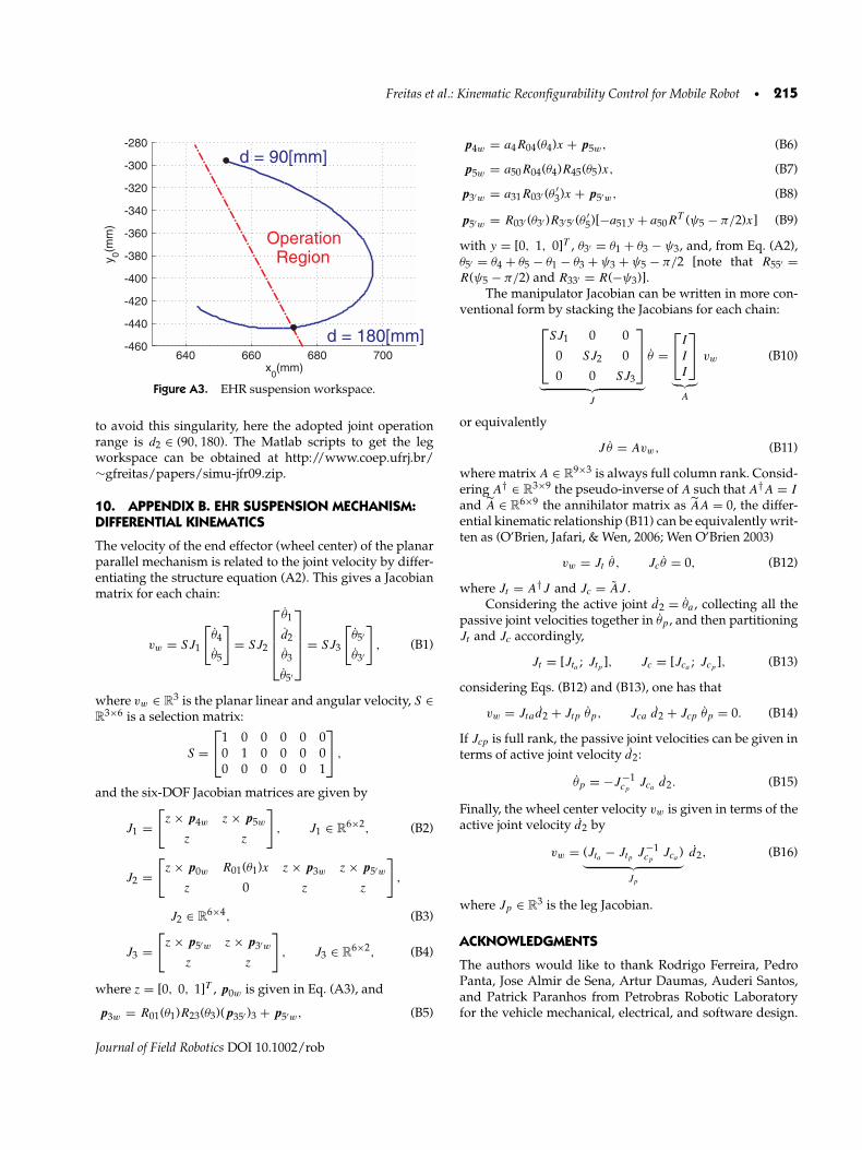
Figure A3 illustrates the suspension workspace, i.e.,the wheel center position p0w in terms of d2 with respectto frame 0. From Figure A3 it is possible to note that thesuspension has a boundary singularity for d2 = 190; thus,



d = 90[mm]

d = 180[mm]

OperationRegion

Figure A3. EHR suspension workspace.

to avoid this singularity, here the adopted joint operationrange is d2 ∈ (90, 180). The Matlab scripts to get the legworkspace can be obtained at http://www.coep.ufrj.br/∼gfreitas/papers/simu-jfr09.zip.

10. APPENDIX B. EHR SUSPENSION MECHANISM:DIFFERENTIAL KINEMATICS

The velocity of the end effector (wheel center) of the planarparallel mechanism is related to the joint velocity by differ-entiating the structure equation (A2). This gives a Jacobianmatrix for each chain:

vw = SJ1

[θ4

θ5

]= SJ2

⎡⎢⎢⎢⎣θ1

d2

θ3

θ5′

⎤⎥⎥⎥⎦ = SJ3

[θ5′

θ3′

], (B1)

where vw ∈ R3 is the planar linear and angular velocity, S ∈

R3×6 is a selection matrix:

S =⎡⎣1 0 0 0 0 0

0 1 0 0 0 00 0 0 0 0 1

⎤⎦ ,

and the six-DOF Jacobian matrices are given by

J1 =[z × p4w z × p5w

z z

], J1 ∈ R

6×2, (B2)

J2 =[z × p0w R01(θ1)x z × p3w z × p5′w

z 0 z z

],

J2 ∈ R6×4, (B3)

J3 =[z × p5′w z × p3′w

z z

], J3 ∈ R

6×2, (B4)

where z = [0, 0, 1]T , p0w is given in Eq. (A3), and

p3w = R01(θ1)R23(θ3)( p35′ )3 + p5′w, (B5)

p4w = a4R04(θ4)x + p5w, (B6)

p5w = a50R04(θ4)R45(θ5)x, (B7)

p3′w = a31R03′ (θ ′3)x + p5′w, (B8)

p5′w = R03′ (θ3′ )R3′5′ (θ ′5)[−a51y + a50R

T (ψ5 − π/2)x] (B9)

with y = [0, 1, 0]T , θ3′ = θ1 + θ3 − ψ3, and, from Eq. (A2),θ5′ = θ4 + θ5 − θ1 − θ3 + ψ3 + ψ5 − π/2 [note that R55′ =R(ψ5 − π/2) and R33′ = R(−ψ3)].

The manipulator Jacobian can be written in more con-ventional form by stacking the Jacobians for each chain:⎡⎢⎣SJ1 0 0

0 SJ2 0

0 0 SJ3

⎤⎥⎦︸︷︷︸

J

θ =⎡⎣I

I

I

⎤⎦︸︷︷︸

A

vw (B10)

or equivalently

J θ = Avw, (B11)

where matrix A ∈ R9×3 is always full column rank. Consid-

ering A† ∈ R3×9 the pseudo-inverse of A such that A†A = I

and A ∈ R6×9 the annihilator matrix as AA = 0, the differ-

ential kinematic relationship (B11) can be equivalently writ-ten as (O’Brien, Jafari, & Wen, 2006; Wen O’Brien 2003)

vw = Jt θ , Jcθ = 0, (B12)

where Jt = A†J and Jc = AJ .Considering the active joint d2 = θa , collecting all the

passive joint velocities together in θp , and then partitioningJt and Jc accordingly,

Jt = [Jta ; Jtp ], Jc = [Jca; Jcp

], (B13)

considering Eqs. (B12) and (B13), one has that

vw = Jtad2 + Jtp θp, Jca d2 + Jcp θp = 0. (B14)

If Jcp is full rank, the passive joint velocities can be given interms of active joint velocity d2:

θp = −J−1cp

Jcad2. (B15)

Finally, the wheel center velocity vw is given in terms of theactive joint velocity d2 by

vw = (Jta − Jtp J−1cp

Jca)︸︷︷︸

Jp

d2, (B16)

where Jp ∈ R3 is the leg Jacobian.

ACKNOWLEDGMENTS

The authors would like to thank Rodrigo Ferreira, PedroPanta, Jose Almir de Sena, Artur Daumas, Auderi Santos,and Patrick Paranhos from Petrobras Robotic Laboratoryfor the vehicle mechanical, electrical, and software design.



This work was partially supported by FAPERJ, CNPq, andPetrobras S.A.

REFERENCES

Chitsaz, H., O’Kane, J., & LaValle, S. (2004, May). Exact Pareto-optimal coordination of two translating polygonal robotson an acyclic roadmap. In IEEE International Conferenceon Robotics and Automation, New Orleans, LA (vol. 4,pp. 3981–3986).

Cunninghan, J., Corke, P., Durrant-Whyte, H., & Dalziel, M.(1999). Automated LHD’s and underground haulagetrucks. Australian Journal of Mining, 51–53.

Davids, A. (2002). Urban search and rescue robots: Fromtragedy to technology. IEEE Intelligent Systems, 17(2),81–83.

Deb, K. (2008). Multi-objective optimization using evolution-ary algorithms. Chichester, UK: Wiley.

dos Reis, N. R. S. (2007a). Suspension system with camber forenvironmental vehicle. Patent Number BR200504231-A.Petrobras SA (PETB).

dos Reis, N. R. S. (2007b). Wheel for vehicle used on differenttypes of terrains. Patent Number BR200504259-A. Petro-bras SA (PETB).

Freitas, G., Lizarralde, F., Hsu, L., & dos Reis, N. R. S. (2009,May). Kinematic reconfigurability of mobile robot onirregular terrains. In IEEE International Conference onRobotics and Automation, Kobe, Japan (pp. 1340–1345).

Galvez, J. A., Estremera, J., & de Santos, P. G. (2003). A newlegged-robot configuration for research in force distribu-tion. Mechatronics, 13(8–9), 907–932.

Ghrist, R., O’Kane, J., & LaValle, S. (2005). Computing Paretooptimal coordinations on roadmaps. International Journalof Robotics Research, 24(11), 997–1010.

Goldstein, H. (1980). Classical mechanics. New York: ColumbiaUniversity.

Grand, C., Amar, F. B., Plumet, F., & Bidaud, P. (2002, Septem-ber). Stability control of a wheel-legged mini-rover. InCLAWAR 5th International Conference on Climbing andWalking Machines, Paris (pp. 323–331).

Grand, C., Amar, F. B., Plumet, F., & Bidaud, P. (2004). Stabil-ity and traction optimization of a reconfigurable wheel-legged robot. International Journal of Robotics Research,23(10–11), 1041–1058.

Guizzo, E. (2008). Dream jobs 2008—Ney Robinson Salvidos Reis: Into the wild. IEEE Spectrum Magazine, 45(2),33–34.

Iagnemma, K., & Dubowsky, S. (2000, September). Mo-bile robot rough-terrain control (RTC) for planetary ex-ploration. In Proceedings of the 26th ASME BiennialMechanisms and Robotics Conference, Baltimore, MD(pp. 10–13).

Iagnemma, K., & Dubowsky, S. (2004). Estimation, motionplanning, and control with application to planetaryrovers. Berlin: Springer-Verlag.

Iagnemma, K., Rzepniewski, A., Dubowsky, S., Pirjanian, P.,Huntsberger, T., & Schenker, P. (2000, November). Mobilerobot kinematic reconfigurability for rough-terrain. SPIE

Sensor Fusion and Decentralized Control in Robotic Sys-tems III, Boston (vol. 4196, pp. 413–420).

Iagnemma, K., Rzepniewski, A., Dubowsky, S., & Schenker, P.(2003). Control of robotic vehicles with actively articulatedsuspensions in rough terrain. Autonomous Robots, 14(1),5–16.

Kim, J., Kim, Y., Choi, S.-H., & Park, I. (2009). Evolutionarymultiobjective optimization in robot soccer system for ed-ucation. IEEE Computational Intelligence Magazine, 4(1),31–41.

Klein, C., & Kittivatcharapong, S. (1990). Optimal force distri-bution for the legs of a walking machine with friction coneconstraints. IEEE Transactions on Robotics and Automa-tion, 6(1), 73–85.

Kumar, V. R., & Waldron, K. J. (1988). Force distribution inclosed kinematic chains. IEEE Journal of Robotics and Au-tomation, 4(6), 657–664.

Lee, C., Kim, S., Kang, S., Kim, M., & Kwak, Y. (2003). Double-track mobile robot for hazardous environment applica-tions. Advanced Robotics, 17(5), 447–459.

Mae, Y., Yoshida, A., Arai, T., Inoue, K., Miyawaki, K., &Adachi, H. (2000, November). Application of locomotiverobot to rescue tasks. In IEEE/RSJ International Confer-ence on Intelligent Robots and Systems, Takamatsu, Japan(vol. 3, pp. 2083–2088).

McGhee, R. B., & Frank, A. A. (1968). On the stability propertiesof quadruped creeping gaits. Mathematical Biosciences,3(3–4), 331–351.

Messuri, D. A. & Klein, C. A. (1985). Automatic body regula-tion for maintaining stability of a legged vehicle duringrough-terrain locomotion. IEEE Journal of Robotics andAutomation, 1(3), 132–141.

Murray, R. M., Li, Z., & Sastry, S. S. (1993). A mathematical in-troduction to robotic manipulation. Boca Raton, FL: CRC.

O’Brien, J. F., Jafari, F., & Wen, J. T. (2006). Determination ofunstable singularities in parallel robots with N-arms. IEEETransactions on Robotics, 22(1), 160–167.

Osborn, J. F. (1989, May). Applications of robotics in haz-ardous waste management. In SME World Conference onRobotics Research, Gaithersburg, MD.

Papadopoulos, E. G., & Rey, D. A. (1996, April). A new measureof tipover stability margin for mobile manipulators. InIEEE International Conference on Robotics and Automa-tion, Minneapolis, MN (vol. 4, pp. 3111–3116).

Roberts, J., Duff, E., Corke, P., Sikka, P., Winstanley, G., &Cunninghan, J. (2000, April). Autonomous control of un-derground mining vehicles using reactive navigation. InIEEE International Conference on Robotics and Automa-tion, San Francisco, CA (vol. 4, pp. 3790–3795).

Sreenivasan, S. V. (1994). Actively coordinated wheeled vehi-cle systems. Ph.D. thesis, Mechanical Engineering Depart-ment, Ohio State University.

Sreenivasan, S. V., & Wilcox, B. H. (1994). Stability and trac-tion control of an actively actuated micro-rover. Journal ofRobotic Systems, 11(6), 487–502.

Wen, J. T., & O’Brien, J. F. (2003). Singularities in three-leggedplatform-type parallel mechanisms. IEEE Transactions onRobotics and Automation, 19(4), 720–727.


Kinematic reconfigurability control for an environmental mobile robot operating in the Amazon rain...

Documents

Transcript of Kinematic reconfigurability control for an environmental mobile robot operating in the Amazon rain...