ADAPTIVE CONTROL OF CONSTRAINED MARKOV CHAINS:CRITERIA AND POLICIES*Eitan Altman and Adam ShwartzElectrical EngineeringTechnion | Israel Institute of TechnologyHaifa, 32000 IsraelABSTRACTWe consider the constrained optimization of a �nite-state, �nite action Markov chain. In theadaptive problem, the transition probabilities are assumed to be unknown, and no prior distributionon their values is given. We consider constrained optimization problems in terms of several costcriteria which are asymptotic in nature. For these criteria we show that it is possible to achievethe same optimal cost as in the non-adaptive case.We �rst formulate a constrained optimization problem under each of the cost criteria andestablish the existence of optimal stationary policies.Since the adaptive problem is inherently non-stationary, we suggest a class of \AsymptoticallyStationary" (AS) policies, and show that, under each of the cost criteria, the costs of an AS policydepend only on it's limiting behavior. This property implies that there exist optimal AS policies.A method for generating adaptive policies is then suggested, which leads to strongly consistentestimators for the unknown transition probabilities. A way to guarantee that these policies are alsooptimal is to couple them with the adaptive algorithms of [3]. This leads to optimal policies foreach of the adaptive constrained optimization problems under discussion.Submitted October 1989. Revised March 1990.* This work was supported in part through United States | Israel Binational Science FoundationGrant BSF 85-00306. 1

1. INTRODUCTION.The problem of adaptive control of Markov chains has received considerable attention in recentyears; see the survey paper by Kumar [18], Hernandez-Lerma [10] and references therein. In thesetup considered there, the transition probabilities of a Markov chain are assumed to depend onsome parameter, and the \true" parameter value is not known. One then tries to devise a controlpolicy which minimizes a given cost functional, using on-line estimates of the parameter. In mostof the existing work, the expected average cost is considered. Recently Sch�al [22] introduced anasymptotic discounted cost criterion. Adaptive optimal policies with respect to the latter criterionwere investigated by Sch�al [23], and a variation of this criterion was considered by Hernandez-Lerma and Marcus [11,13,12]. Concerning the Bayesian approach to this problem, see Van Hee [25]and references therein.Since we adopt a non-Bayesian framework it is natural, in order to formulate an adaptiveproblem, to consider only those cost criteria which do not depend on the �nite-time behavior of theunderlying controlled Markov chain. For such criteria, it may be possible to continuously improvethe policy, using on-line parameter estimates, so as to obtain the same (optimal) performance asin the case where all parameters are known. We consider the well-known Expected Average costand Sample Average (or ergodic) cost, the Sch�al discounted cost, and introduce a new AsymptoticDiscounted cost. In Section 2 we de�ne these cost functionals and formulate a constrained and anadaptive constrained optimization problem for each cost structure. For example, the Average-Costconstrained problem amounts to minimizing an average cost, subject to inequality constraints interms of other average cost functionals.Adaptive policies for constrained problems were �rst introduced by Makowski and Shwartz[19,24] in the context of the expected average cost and under a single constraint. They rely on theLagrange approach of Beutler and Ross [4], which is limited to a single constraint. The generalconstrained adaptive control problem of a �nite state chain under the expected average cost isconsidered by Altman and Shwartz [3]. Using the \Action Time-Sharing" (ATS) policies, theyobtain optimal adaptive policies. In Section 3 we recall the de�nition of these policies and showthat they are useful for the sample average cost as well. We obtain some useful characterizationsof the average and the expected average costs.The adaptive control paradigm is roughly the following. At each decision epoch;(i) Compute some estimate of the unknown parameters,2

(ii) Use these values to compute a control policy,(iii) Apply the policy of (ii) and repeat.The \certainty equivalence" approach to the computation in step (ii) is to treat the valuesprovided in (i) as the correct parameter values, and compute the corresponding optimal (stationary)control. There are several drawbacks to this approach; �rst, the complexity of computing optimalpolicies is very high [10]. In the constrained case, the optimal policy may be a discontinuousfunction of the parameter [3]. A more fundamental consideration is the following. Clearly a poorestimate may result in a bad choice of control. Such a choice may in turn suppress estimation, sayby using only such control actions which do not provide new information. The use of a stationarypolicy may cause the algorithm to \get stuck" at an incorrect value of the parameter, hence alsoat a suboptimal policy.We propose the following approach to the adaptive control problem. We �rst show that thecosts depend only on limiting properties of the control. This makes it possible to apply \forcedchoices" of controls which are not optimal, but enhance estimation (see e.g. [18]). Consistentestimation is guaranteed by making these choices su�ciently often. We show that it is possibleto achieve consistent estimation without changing the limiting properties. Finally, we choose aconvenient implementation of a policy, incorporating the \forced choices" and possessing the correctlimiting behavior to ensure optimality.Section 3 treats the average cost and serves as a template for the development in this paper,and below we describe the analogue development in Section 3 vs. Sections 4{7. In Section 3 we �rstrecapitulate the existence of optimal stationary policies for the (non-adaptive) constrained averagecost problem. It is well known that this problem can be solved via a linear program (see e.g. [15],which extends the linear program used for the non constrained case [8 p. 80]). This suggests amethod for the computation in (ii). These steps are followed for the other cost criteria in Section4, where we show that there exists an optimal stationary policy for the constrained (non-adaptive)problem, and in Section 5 where we show that the Linear Program of [15] applies also for theasymptotic discounted cost. An extension of another Linear Program [8 p. 42] is shown to providea method of computing stationary policies for the constrained non-adaptive problem under thediscounted and the Sch�al cost criteria. Unlike the non-constrained case, the optimal policies forthe discounted problems depend on the initial state.Section 3 proceeds to discuss the ATS class of policies (which includes the stationary policies)for which limits of the conditional frequencies (3.3) exist. We then show (following [3]) that average3

costs depend only on these limits. This provides conditions under which forced choices do not a�ectthe �nal average cost. ATS policies are not applicable to the other cost criteria, since the othercosts are not determined by these limits. The key concept for these cost criteria is the new andmore re�ned limits introduced in (1.2). Policies possessing these limits are called \AsymptoticallyStationary" (AS). In Section 6 we show that under those policies there exists a limiting distributionfor the state of the process, which coincides with the invariant distribution under the correspondingstationary policy. Moreover, for each of the cost criteria, the cost of an AS policy equals the costunder the corresponding stationary policy. It follows that AS policies possess the asymptoticproperties needed to achieve optimality, while retaining the exibility which is needed to obtainconsistent estimation; they are thus useful for the adaptive problems.In Section 7 we construct an optimal adaptive policy. To do so, we �rst show how to computeestimates of the unknown transitions from the history of previous states and actions. We then showhow to compute the (sub-optimal) stationary policy that is used till the next estimate is obtained.This stationary policy incorporates \forced choices" of actions for the sake of enhancing estimation.We �nally show that this scheme yields an AS policy that is optimal for the constrained adaptiveproblem.The model.Let fXtg1t=0 be the discrete time state process, de�ned on the �nite state space X = f1; :::; Jg;the action At at time t takes values in the �nite action space A; X and A are equipped with thecorresponding discrete topologies 2X and 2A. Without loss of generality, we assume that in anystate x all actions in A are available. We use the space of paths fXtg and fAtg as the canonicalsample space , equipped with the Borel �-�eld B obtained by standard product topology.Denote by Ht := (X0; A0;X1; A1; :::;Xt; At) the history of the process up to time t. If the stateat time t is x and action a is applied, then for any history ht�1 2 (X�A)t of states and actionstill time t� 1, the next state will be y with probabilityPxay := P (Xt+1 = y j Xt = x;At = a) = P (Xt+1 = y j Ht�1 = ht�1;Xt = x;At = a) (1:1)A policy u in the policy space U is a sequence u = fu0; u1; :::g, where ut is applied at time epoch t,and ut(� j Ht�1;Xt) is a conditional distribution over A. Each policy u and initial state x inducea probability measure Pux on f;Bg. The corresponding expectation operator is denoted by Eux .A Markov policy u 2 U(M) is characterized by the dependence of ut(� j Ht�1;Xt) on Xt only,i.e. for each t, ut(� j Ht�1;Xt) = ~ut(� j Xt). A stationary policy g 2 U(S) is characterized by a4

single conditional distribution pg�jx := u(� j Xt = x) over A; under g, Xt becomes a Markov chainwith stationary transition probabilities, given by P gxy := Pa2A pgajxPxay. The class of stationarydeterministic policies U(SD) is a subclass of U(S) and, with some abuse of notation, every g 2U(SD) is identi�ed with a mapping g : X! A, so that pg�jx = �g(x)(�) is concentrated at the pointg(x) in A for each x.Call a policy u Asymptotically Stationary (AS) if for some stationary policy g,limt!1Pux (At = ajXt = y;Ht�1) = pgajy Pux a:s: (1:2)for any initial state x and all a and y. Any policy satisfying (1.2) is denoted by g, and G(g) is theset of such policies corresponding to g. The class of policies such that (1.2) holds for some g inU(S) is denoted by U(AS).Throughout the paper we impose the following assumption:A1: Under any stationary deterministic policy g 2 U(SD), the process Xt is a regular Markovchain,(i.e. there are no transient states, and the state space consists of a single ergodic non-cyclic class).Under this assumption, each stationary policy g induces a unique stationary steady statedistribution on X, denoted by �g(�).The following notation is used below: �a(x) is the Kronecker delta function. For an arbitraryset B, 1[B] is the indicator function of the set and cl B the closure of B. For any function � : B ! IRwe de�ne ��(y) := maxf0;��(y)g; y 2 B. When B is a �nite set we denote by jBj the cardinalityof the set (i.e. the number of elements in B) and by S(B) the (jBj � 1)-dimensional real simplex,i.e. S(B) := fq : q 2 IRjBj; PjBji=1 qi = 1; 0 � qi � 1 for all ig. For vectors D and V in IRK ,the notation D < V stands for Dk < Vk ; k = 1; 2; : : : ;K:. For two matrices �; P of appropriatedimensions the notation � � P stands for summation over common indices.2. PROBLEM FORMULATIONLet C(x; u) and D(x; u) := fDk(x; u) ; 1 � k � Kg be cost functions associated with eachpolicy u and initial state x. The precise de�nitions of several cost functions of interest are givenbelow. The real vector V := fVk ; k = 1; :::;Kg is held �xed thereafter. Call a policy u feasible ifDk(x; u) � Vk ; k = 1; 2; : : : ;K5

The constrained optimization problem is:(COP) Find a feasible v 2 U that minimizes C(x; u)The unconstrained problem (where K = 0) is denoted by OP.The adaptive constrained optimization problem ACOP is de�ned as follows. The values ofthe transition probabilities Pxay are unknown, except that assumption A1 is known to hold. Theobjective is still to �nd an optimal policy forCOP, but based on the available information, assumingthat no a-priori information about the values of the fPxayg is available. In choosing the control tobe used at time t, the only available information are the observed values fHt�1;Xtg. The paradigm(i){(iii) in adaptive control is then to use the observations to obtain information about the valuesof fPxayg, leading to computation of an adaptive policy. The notation Pxay here stands for thetrue but unknown values of the transition probabilities, and similarly for the notation P , E and �g.Let c(x; a), d(x; a) := fdk(x; a) ; k = 1; :::;Kg be real (IRK) valued instantaneous cost func-tions, i.e. costs per state-action pair. We shall use the following cost functions from X � U toIR:The expected average costs:Cea(x; u) := limt!1 1t+ 1Eu " tXs=0 c(Xs; As) j X0 = x# (2:1a)Dkea(x; u) := limt!1 1t+ 1Eu " tXs=0 dk(Xs; As) j X0 = x# k = 1; :::;K (2:1b)Let 0 < � < 1 be a discount factor. The expected discounted costs:Ced(x; u) := Eu " 1Xt=0 �tc(Xt; At) j X0 = x# (2:2a)Dked(x; u) := Eu " 1Xt=0 �tdk(Xt; At) j X0 = x# k = 1; :::;K (2:2b)As noted above, in the adaptive case, we would like to obtain the same optimal value ofC(x; u), despite the lack of information. Clearly, under the discounted cost criteria we cannot hopeto obtain the same costs as when the fPxayg are known, since the actions taken at each �nite timet will generally be sub-optimal. Therefore, the performance in terms of the cost functions Ced andDed will be degraded with respect to the case where all parameters are known. Moreover, since6

we work in the framework of non-Bayesian adaptive control (no prior information is given on theunknown parameters), there is no natural way to de�ne optimal adaptive policies with respect tothis cost criterion (see discussion in [10] Section II.3). This motivates the following \asymptotic"de�nitions; consider the N-stage expected discounted costs:CNed(x; u) := Eu " 1Xt=N �t�N c(Xt; At) j X0 = x# (2:3a)DN;ked (x; u) := Eu " 1Xt=N �t�Ndk(Xt; At) j X0 = x# k = 1; :::;K (2:3b)De�ne the asymptotic expected discounted costCaed(x; u) := limN!1CNed(x; u) (2:4)with similar de�nitions for Dkaed(x; u) ; k = 1; 2; : : : ;K.The constrained optimization problems COPea, COPed, COPNed and COPaed are de�ned by usingthe appropriate de�nitions of the costs in the general de�nition of COP. We denote by, e.g., ACOPeathe adaptive problem that corresponds to COPea, with a similar notation for the other relevantcost criteria.Inspired by Sch�al [23], de�ne the asymptotic constrained problem in the sense of Sch�al COPsdas follows. Let g 2 U(S) be an optimal stationary policy for COPed; we prove the existence of sucha policy in Theorem 4.3. A policy u is feasible for COPsd iflimN!1 �DN;ked (x; u)� Eu[Dked(XN ; g) j X0 = x]� � 0 ; k = 1; :::;K (2:5a)A policy u is optimal for COPsd if it is feasible andlimN!1 ��CNed(x; u)� Eu[Ced(XN ; g) j X0 = x]�� = 0 (2:5b)This concept was �rst used by Sch�al [23] for the unconstrained adaptive problem. The version in(2.5) is the one used by Hernandez-Lerma, Marcus et al: see [10] and references therein. The reasonwe prefer to use the version of [10] is that for this case there exists an optimal stationary policy forthe constrained problem whenever there exists a feasible policy (see Theorem 4.9), whereas underthe de�nition of [23] an optimal policy for the constrained problem may not exist (see Appendix).7

In the unconstrained problems treated in [10,23], the optimal policy is independent of theinitial state, and so Eux [Ced(XN ; g)] is the minimal cost, given the initial distribution of XN . Asis shown in Example 5.3, the optimal policy of COPed depends, in general, on the initial state.Thus, an optimal COPsd policy tries to imitate, in the limit, the behavior of the optimal policycorresponding to the initial state x. Consequently, Eux [Ced(XN ; g)] is not necessarily the minimalcost, given the initial distribution of XN since g may not be optimal for this \initial" distribution.Moreover, it is possible that if u� is an optimal policy for COPsd, then DN;ked (x; u�) > Vk + � forsome x and � > 0 and for all N . In COPaed, in the period 0 � t � N we attempt to obtain the\initial" distribution Pu(XN j X0 = x) which is best for obtaining good performance from t = Nonwards. We also require that (in the limit) the constraints are satis�ed.Finally, the sample average costs are the random variables, given byCav := limt!1 1t+ 1 tXs=0 c(Xs; As) (2:6a)Dkav := limt!1 1t+ 1 tXs=0 dk(Xs; As) ; k = 1; :::;K (2:6b)A policy u is feasible for COPav ifDkav � Vk Pux a.s. ; x 2 X ; k = 1; 2; : : : ;K (2:7a)A policy v is optimal for COPav if it is feasible, and if for every feasible policy u and every constantM , Pux (Cav �M) > 0 implies Cav �M P vx a.s. (2:7b)The main results of this paper can now be stated:Theorem 2.1: Under A1, if COPea (resp. COPed, COPNed , COPaed, COPsd or COPav) isfeasible, then there exists an optimal stationary policy for COPea (resp. COPed, COPNed , COPaed,COPsd or COPav).Proof: The result for COPea is well known [8,15]. This and the other results are given in Theorems3.1, 4.3, 4.3, 4.7, 4.9 and 4.1 respectively.Theorem 2.2: Under A1, if g in U(S) is optimal for COPea, COPaed, COPsd or COPav thenany g in G(g) is also optimal for the respective problem.8

Proof: This claim is established in Theorem 6.4.The computation of optimal stationary policies is discussed in Section 5, where a new LinearProgram for COPed and COPsd is obtained. We show that the well-known Linear Program whichsolves COPea also provides an optimal solution for COPav and COPaed.In Section 7 we provide a method for modifying an adaptive algorithm so as to obtain stronglyconsistent estimation of the transition probabilities. The modi�ed policy is an AS policy with thesame limits, so that by Theorem 2.2 this modi�cation does not change its optimality properties.Explicit optimal adaptive policies can be obtained by using the estimation scheme of Section7, combined with the methods of [3].3. AVERAGE COSTS; frequencies and ATS policies.In this section we investigate the average cost criteria. For the expected average cost, theconstrained problem has been studied extensively. In particular, the following Theorem is provedin [16], [15] or [2, Theorem 2.9].Theorem 3.1: Assume A1, and that COPea is feasible. Then there exists an optimal stationarypolicy for COPea.The computation of the optimal stationary policy is presented in Section 5.1.Remark: In the multichain case an optimal stationary policy may not exist. For that case,Hordijk and Kallenberg [15] provide a method of computing an optimal Markovian policy. Rossand Varadarajan [21] have studied a constrained problem that involves minimization of the expectedaverage cost subject to a single constraint of the sample average type. They obtain an optimalstationary policy for the unichain case and �-optimal stationary policies for the multi-chain case.Since adaptive policies cannot usually be stationary, a larger class of policies is needed forACOPea. It will be convenient to mimic, in some asymptotic sense, the behavior of stationarypolicies. The class of \Action Time Sharing" (ATS) policies was introduced in ([1,2]) and was usedto solve ACOPea in [3]. We show in Section 3.3 that this approach also solves ACOPav .The development of ATS policies proceeds through the following steps. Following Derman [8 p.89] we show that the expected state action frequencies (see de�nitions below) determine the expectedaverage cost. Hordijk and Kallenberg [16, 15] used the expected frequencies in solving COPea. Then9

we establish (Lemma 3.2) the measurability of the state-action frequencies ([8 Chapter 7]) and showbelow that they determine the sample average cost.Altman and Shwartz [2] extended the analysis of the expected average case to a countablestate space, and introduced a more basic quantity, the conditional frequencies, which determinethe frequencies, and hence the sample average and the expected average costs (see also [1] and[3]). ATS policies are de�ned through the conditional frequencies. The analysis in Section 6 ofthe Asymptotically Stationary (AS) policies which are needed for other cost criteria, also relies onthese results.3.1. State-Action Frequencies.The state action (sa) frequency fTsa is a random vector fTsa : ! S(X � A) de�ned byfTsa(y; a) := 1T+1PTr=0 1fXr = y;Ar = ag. The value of fTsa(y; a;!) is the frequency at which theevent of being at state y and choosing action a occurs by time T . We de�ne similarly the state(s) frequency fTs as the frequency at which the event of being at state y occurs till time T . It is arandom vector fTs : ! S(X) de�ned by fTs (y) := 1T+1PTr=0 1fXr = yg.Denote by �fTsa(x; u) and �fTs (x; u) the vectors whose components are given respectively by�fTsa(x; u; y; a) := Eu[fTsa(y; a)jX0 = x], and �fTs (x; u; y) := Eu[fTs (y)jX0 = x]. Let �Fsa(x; u) denotethe set of all accumulation points of �fTsa(x; u) as T ! 1, and �Fs(x; u) the set of accumulationpoints of �fTs (x; u) as T !1.Similarly, the multifunction Fsa is a mapping from whose values are subsets of S(X �A) andis given by the (random) set of accumulation points of fTsa as T ! 1. The multifunction Fs is amapping from whose values are subsets of S(X) and is given by the set of accumulation pointsof the vectors fTs as T ! 1. The multifunction (multivalued random vector) Fsa is said to beBorel-measurable ([22, Section 9] or [10, Appendix D]) if the setF�1sa [B] := f! : Fsa(!) \ B 6= �g 2 Bfor every closed subset B in the standard Borel �-�eld on S(X �A). The measurability of Fs issimilarly de�ned in terms of Borel subsets of S(X). The measurability of Fsa and Fs is discussed inLemma 3.2 below. Since the sets �Fsa(x; u) �Fs(x; u) (Fsa(!) and Fs(!)) are all sets of accumulationpoints and are all bounded, they are all compact sets (for each !).De�ne for any given set of policies U 0 the set of achievable expected state action frequenciesLx(U 0) := [u2U 0 �Fsa(x; u). In particular, the set of all achievable expected frequencies is denotedby Lx := [u2U �Fsa(x; u). 10

The following Lemmas 3.2-3.3 establish some basic properties of the state action frequenciesand relate them to the cost achieved by the policies.Lemma 3.2: Under A1;(i) The class of stationary policies is complete, i.e. Lx(U(S)) = Lx for every initial state x.Moreover, L := Lx is independent of x.(ii) Fsa and Fs are Borel measurable.(iii) Under any policy u, Fsa � L(U(S)) Pux a:s.Proof: The �rst claim is proved in Derman [8, pp. 95] (a generalization to the countable stateand action spaces is obtained in [2, Theorem 3.1]). We prove (ii) for Fs, as the proof for Fsa is thesame. Pick any closed subset B in the standard Borel �-�eld on S(X). Note thatFs(!) = \1k=1 cl �[1t=kff ts(!)g(see e.g. [7]). HenceF�1s (B) = f! : \1k=1 = \1k=1f! : cl �[1t=kff ts(!)g \ B 6= �gLet fBng11 be a sequence of open sets containing B, with \1n=1Bn = B. Since B is closed,F�1s (B) = \1k=1f! : \1n=1 �[1t=kf ts(!)\ Bn� 6= �g = \1k=1 \1n=1 [1t=kf! : ff ts(!)g \ Bn 6= �g :Since f ts are clearly (measurable) random variables, it follows that f! : f ts(!) 2 Bng 2 B and henceF�1s (B) 2 B, which establishes (ii). In view of (ii), (iii) follows from Derman [8, pp. 98].3.2. Costs and frequencies.We show below that the state-action frequencies (expected frequencies) determine the cost Cav(respectively Cea). This result obviously applies to Dav and Dea.Lemma 3.3: Under A1, for every policy u 2 U and any instantaneous cost function c,(i) there exists some �� 2 �Fsa(x; u) for which the cost Cea(x; u) obeysCea(x; u) =Xy Xa c(y; a)��(y; a) (3:1)(ii) there exists some random variable �� with ��(!) 2 Fsa(!) for which the cost Cav obeysCav =Xy Xa c(y; a)��(y; a): (3:2)11

Remark: The main issue in (ii) is to show that �� can be chosen so that it is a measurablemappingfrom f;Bg to S(X�A).Proof: The �rst claim is in Derman [8, pp. 89]. To prove (ii), de�ne the function v : S(X�A)! IRby v(�) := c � � :=Px;a c(x; a)�(x; a). ThenCav = limt!1 1t+ 1 tXs=0 c(Xs; As) = limt!1 c � f tsaSince for each !, any accumulation point of c � f tsa can be expressed as c � � with �(!) 2 Fsa(!), weobtain Cav = sup�2Fsa c � � = max�2Fsa v(�)where the second equality follows from the compactness (for each !) of the range of Fsa. Sincev is continuous and since Fsa is Borel measurable with compact range, it follows from a standardMeasurable Selection Theorem (see [10, Appendix D] or [22, Section 9]) that there exists a randomvariable (called a Selector) �� with ��(!) 2 Fsa(!) such that v(��) = c � �� = max�2Fsa v(�).3.3. Conditional frequencies and ATS policies.The conditional frequency f tc is a collection ff tc(ajy); all a; yg, so that the components of therandom vector f tc : ! S(A)J (with J = jXj) are given byf tc(ajy) := Pts=0 1fXs = y;As = agPts=0 1fXs = yg (3:3)if Pts=0fXs = yg = 0 set f tc(ajy) := 1jAj . This quantity represents the frequency that action a isused conditioned on state y being visited.The set of limit points of f tc as t!1 is denotes by Fc. If only one limit exists then it is denoted byfc. Lemma 3.5 below states that the conditional frequencies determine the state-action frequenciesand the expected frequencies, hence they determine the cost. The conditional frequencies are thekey quantities for the controller, since they can be directly steered to the desired values. Forinstance, if we need to obtain f(ajy) = 0:2 for some a; y then one possibility for achieving this isto use action a every �fth visit to state y. That this is possible, is a consequence of the followingLemma, whose proof is available in [1, Lemma 4.1] or [2, Corollary 5.3]. Note that there is no suchdirect way to control the (expected) state-action frequencies.12

Lemma 3.4: Under A1, for any policy u, each state y 2 X is visited in�nitely often Pux a.s.A policy u is called an ATS policy corresponding to some stationary policy g if Fc is a singleton,with fc(ajy) = pgajy Pux a.s.Lemma 3.5: Assume A1, and �x some stationary policy g. If under a policy u, fc(ajy) =pgajy Pux a:s: Then(i) Fsa and �Fsa are singletons, and for all a, y, fsa(y; a) = �fsa(x; u; y; a) = pgajy�gy Pux a.s.(ii) For any initial state x, Cea(x; g) = Cea(x; u) = Cav Pux a:s. and Cea(x; g) = Cav P gx a:s.Proof: The �rst claim is proved in [2, eq. (4.5)] (see also [5, p. 969]). The second claim thenfollows from Lemma 3.3.From the de�nition it is clear that these conditional frequencies are not sensitive to the use of\bad" (non-optimal) controls at some initial �nite time interval, nor are they a�ected by the use ofnon-optimal controls provided that the frequency at which they are used decreases to zero. The costfunctions Cea and Cav also have these properties due to their de�nition as time-averages. Thus it isto be expected that only Cesaro properties of the control should in uence the costs. This propertymakes ATS policies attractive for ACOPea, since we do not need to know the optimal stationarypolicy g at any �nite time; a (strongly) consistent estimator of pgajy su�ces for optimality. On theother hand, ATS policies facilitate estimation through probing, i.e. by testing non-optimal actionswithout a�ecting the cost. Such policies were indeed used in [3] to solve ACOPea.It is shown in Theorem 4.1 that the stationary policies are optimal for COPav . Moreover,the stationary policy g which is optimal for COPea is also optimal for COPav . It then followsfrom Lemma 3.5 (ii) that the ATS policy that solves ACOPea also solves ACOPav . Therefore themethod described in [3] to solve ACOPea is optimal for ACOPav as well.ATS policies are not adequate for the other cost criteria introduced in Section 2, since theconclusion (ii) of Lemma 3.5 does not hold for cost criteria (even asymptotic) which are based ondiscounting rather than time average. We therefore have to develop other policies in order to obtainan adaptive method that can be applied to all ACOP. In the next section we show that stationarypolicies are optimal for all cost criteria under consideration. We then develop, in Section 6, theAsymptotically Stationary policies. 13

4. STATIONARY POLICIES: OPTIMALITYThe optimality of stationary policies for COPea is discussed in the beginning of Section 3 (seeTheorem 3.1). In this section we prove the optimality of stationary policies for the other costcriteria under consideration.4.1. The sample average costTheorem 4.1: Assume A1. Then(i) COPav is feasible if and only if COPea is feasible.(ii) The stationary policies are optimal for COPav .(iii) A stationary policy is optimal for COPea if and only if it is optimal for COPav.Proof: Since under a stationary policy g, Dav = Dea(g) P gx a.s. and similarly for C, (iii) followsfrom (i) and (ii).If COPea is feasible, then there exists a feasible stationary policy. But under a stationarypolicy g, Dav = Dea(g) P gx a.s., so COPav is feasible.Now assume COPav is feasible. By Fatou's Lemma, since clearly 1t+1Pts=0 dk(Xs; As) isbounded, limt!1Eux 1t+ 1 tXs=0 dk(Xs; As) � Eux limt!1 1t+ 1 tXs=0 dk(Xs; As) = EuxDkav � Vkand (i) follows.Let v be a stationary optimal policy for COPea and �x some policy u and initial state x. LetY := f! : Cav < Cea(x; v); Dav � V g. Fix a selector � 2 Fsa that satis�es Cav = � � c. Fix anarbitrary !0 2 Y and denote � := �(!0). Let tn be an increasing subsequence of times, such that� := limn!1 f tnsa (!0).Claim: � =2 L. To establish the claim by contradiction, assume � 2 L. Then there exists a stationarypolicy g such that �Fsa(x; g) = f�g. By de�nition of Y and � it follows that� � c = Cea(x; g) < Cea(x; v)Dkea(x; g) = � � dk � limt!1 f tsa(!0) � dk � VkThis contradicts the optimality of v, which establishes the claim.14

From this it follows that Pux (Fsa 6� Lx(S)) � Pux (Y ). However by Lemma 3.2 (see Derman [8p. 98]), for any policy u, Pux (Fsa 6� Lx(S)) = 0, so that necessarily Pux (Y ) = 0. Since u is arbitraryand Cea(x; v) = Cav and Dea(x; v) = Dav P vx a:s:, (ii) holds.4.2. The expected discounted costWe begin by de�ning some basic quantities that play an important role in the expected dis-counted cost. De�ne the matrix f��sa(x; u; y; a)gy;a by��sa(x; u; y; a) := 1Xt=0 �tPu(Xt = y;At = ajX0 = x) (4:1)These quantities determine the cost in the following way: for each instantaneous cost c(y; a),y 2 X; a 2 A, the overall cost has the representation (see [6]):Ced(x; u) = Xy2X;a2A c(y; a)��sa(x; u; y; a) (4:2)and similarly for Ded.This representation was suggested and investigated by Borkar [6] who developed a similarrepresentation also for �nite time cost criteria and for the exit problem. In his paper Borkarconsiders a countable state space and a compact action space. He calls the quantity ��sa \occupationmeasure". Borkar's approach is somewhat di�erent, in that he de�nes the occupation measurethrough the cost representation and not explicitly through (4.1).Let L�x denote the set of matrices f��sa(x; u; y; a)gy;a achieved by all policies in U , and L�x(S)the set of matrices f��sa(x; u; y; a)gy;a achieved by all policies in U(S).Lemma 4.2: Assume that under any policy in U(SD), the state space includes a single recurrentclass, where the structure is independent of the policy. Then L�x = L�x(S), and is closed and convex.Proof: See Borkar [6].Theorem 4.3: Under A1 the stationary policies are optimal for COPed and COPNed .Proof: The claim for COPed follows immediately from (4.2) and Lemma 4.2; in fact, this holds evenif we relax Assumption A1 to allow some �xed transient states. In order to prove the second claimconsider the process Xt de�ned on the enlarged state space fX�f1; 2; : : : ; Ng g and the same action15

space A. Let the transition probability be given by: Pfx;jgafy;lg = Pxay for l = j +1 or j = l = N ,and 0 otherwise. Let c(fx; jg; a) = 0 for j 6= N and c(fx;Ng; a) = ��N c(x; a) with the analoguede�nition for dk. Then clearly for any policy u and initial state x, CNed(x; u) = Ced(fx; 1g; u) andDN;ked (x; u) = Dked(fx; 1g; u). This process satis�es the hypotheses of Lemma 4.2, so that the prooffor COPNed follows immediately from the proof for COPed.4.3 The asymptotic expected discounted costTheorem 4.4: Under A1, for any stationary policy g, Caed(x; g) = [1 � �]�1Cea(x; g), andDkaed(x; g) = [1� �]�1Dkea(x; g) ; k = 1; 2; : : : ;K.Proof: For any policy u, note that CNed(x; u) has the representation:CNed(x; u) = Eu[ 1Xt=N �t�N c(Xt; At)jX0 = x]= 1Xt=N �t�NXy;a c(y; a)Pu(Xt = y;At = ajX0 = x) (4:3)Since for any stationary policy the limit �g(y; a) := limt!1 P gx (Xt = y;At = a) exists,limt!1Xy;a c(y; a)P g(Xt = y;At = ajX0 = x) =Xy;a c(y; a)�g(y)pgajy = Cea(g; x) (4:4)(see Lemma 3.5). It then follows from (4.3) thatCaed(x; g) := limN!1CNed(x; g) = [1� �]�1Xy;a c(y; a)�g(y)pgajy = [1� �]�1Cea(x; g) (4:5)The derivation for Dkaed is identical.In order to establish the existence of an optimal stationary policy for COPaed we need thefollowing Lemmas. For any real valued vector z 2 IRjXj, let kzk1 :=Py2X jz(y)j . Let �(�) be anydistribution on X, and recall the convention (� � P )(y) =Px �(x)Pxy.Lemma 4.5: Let P = fPxyg be the transitions of a regular Markov chain on X, with invariantmeasure �. If Pxy � �0 > 0 for all x; y 2 X, then k� � P � �k1 � (1� �0)k� � �k1.16

Proof: k� � P � �k1 = k(� � �) � Pk1 =Xy jXx [�(x)� �(x)]Pxyj (4:6)k� � �k1 =Xx j(�(x)� �(x)j =Xx j�(x)� �(x)jXy Pxy =Xx Xy j�(x)� �(x)jPxy (4:7)Since Px[�(x)� �(x)] = 0, we have Px[�(x)� �(x)]+ = Px[�(x) � �(x)]� and we obtain aftersome algebrak� � �k1 � k� � P � �k1 =Xy Xx 2[�(x)� �(x)]� � Pxy � 2�0Xx [�(x)� �(x)]� = �0k� � �k1 (4:8)The Lemma now follows from (4.8).Lemma 4.6: Under A1, there exists a single constant � < 1, independent of x and of g 2 U(S),and an integer M such that kP g(Xt = �jX0 = x)� �gk1 � �t�M for all t > M .Proof: A1 implies that under any stationary deterministic g, fXtg is a regular Markov chain.Hence (see [17]) for some integer M(g), [P g]M(g) has all components nonzero. Furthermore, sinceU(SD) is a �nite set, then there is an integer M such that [P g]M has all components strictlypositive for any g 2 U(SD), and is a transition matrix for a regular Markov chain with invariantmeasure �g. Since U(SD) is a �nite set, �00 := minf f[P g]Mgyz : g 2 U(SD); y; z 2 Xg > 0.Now enumerate the stationary deterministic policies as fg1; : : : ; gjU(SD)jg. Fix g in U(S); thenP g =PjU(SD)ji=1 qiP gi where qi � 0 and Pi qi = 1. Thereforef[P g]Mgyz � jU(SD)jXi=1 qMi f[P gi ]Mgyz � jU(SD)j�M�00 := �0By Lemma 4.5 applied to the transition matrix [P g]M it follows thatk� � [P g](n+1)M � �gk1 � (1� �0)k� � [P g]nM � �gk1for any initial distribution �(�) and any g 2 U(S). Hencek� � [P g]nM � �gk1 � (1� �0)nuniformly in g 2 U(S) and in �. Thus for t = nM + l where 0 � l < M we havek� � [P g]t � �gk1 = k (� � [P g]l)[P g]nM � �gk1 � (1� �0)n � (1� �0)(t=M)�117

and the result follows.Theorem 4.7: Under A1, if COPaed is feasible then there exists an optimal stationary policy.Proof: Let gn be an optimal stationary policy for COPned and let u be any (not necessarilystationary) feasible policy for COPaed, i.e. Daed(x; u) � V . By de�nition,Caed(x; u) = limN!1CNed(x; u)Thus there exists some increasing sequence of integers nl such thatCaed(x; u) = liml!1Cnled(x; u) (4:9)Since A is �nite, there is some subsequence nm of nl such that for all y, gnm(�; y) converges to somedistribution g(�; y). By Theorem 4.4 we have:Caed(x; g) = [1� �]�1Cea(x; g) =limm!1[1� �]�1Cea(x; gnm) = limm!1Caed(x; gnm) (4:11)where the second equality follows from the representation (4.4) since �g0 is continuous in g0 (seee.g. [14]). Now by (4.3),j Caed(x; gnm)� Cnmed (x; gnm) j� supv2U(S) j Caed(x; v)� Cnmed (x; v) j� supv2U(S) 1Xt=nm �t�nmXy;a jc(y; a)j � pvajy j P vx (Xt = y)� �v(y) jHowever, by Lemma 4.6 j P vx (Xt = y)� �v(y) j! 0 as t!1, uniformly in v. ThereforeCaed(x; g) = [1� �]�1Cea(x; g) = limm!1Cnmed (x; gnm) (4:12)Similarly for Daed we obtain:Daed(x; g) = limm!1Dnmed (x; gnm) (4:13)18

On the other hand we have from (4.9)Caed(x; u) = limm!1Cnmed (x; u) (4:14)Clearly, by de�nition of Daed, Daed(x; u) � limm!1Dnmed (x; u) (4:15)Since Cnmed (x; gnm) � Cnmed (x; u) we obtain from (4.12) and (4.14) that Caed(x; g) � Caed(x; u). Sim-ilarly, (4.13) and (4.15) imply Daed(x; g) � Daed(x; u). Thus, for every policy there is a stationarypolicy with better performance. To conclude note that the continuity of g ! Caed(g) establishedin (4.11) together with the compactness of the space of stationary policies imply the existence ofan optimal stationary policy.The connection between optimal policies for COPea, COPav and COPaed is now summarized.Lemma 4.8: Consider problems COPea and COPav with constraints given by V , and problemCOPaed with constraints given by [1 � �]�1 � V . Under A1, if a stationary policy v is optimal forone of the problems, then it is optimal for all of them.Proof: Recall that there exist stationary optimal policies for COPea, COPav and COPaed (The-orem 3.1, 4.1 and 4.7 resp.). The relation between COPea and COPav is established in Theorem4.1. The relation between COPaed and COPea is immediate from Theorem 4.4.4.4 Sch�al optimalityTheorem 4.9: Assume A1. If COPsd is feasible, there exists an optimal stationary policy forCOPsd. If COPed is feasible and g is an optimal stationary policy for COPed, than g is optimalfor COPsd.Proof: If COPsd is feasible, then by de�nition so is COPed. Thus the �rst claim follows from thesecond. If g is optimal for COPed then by de�nition it is optimal for COPsd.Note that while there is a stationary policy which is optimal for COPea, COPav and COPaeduniformly in the initial conditions, this is not the case for COPsd. As is shown in Example 5.3, foreach initial condition the optimal stationary policy may be di�erent.19

5. COMPUTATION OF OPTIMAL POLICIESIn this Section we show that optimal policies for COPea, COPav , COPaed and for COPed,COPsd (which may be found in U(S), according to the results of Section 4) can be obtained bysolving the appropriate Linear Programs. A similar solution for COPNed is obtained through theembedding described in the proof of Theorem 4.3.5.1 Optimal policies for COPea, COPav, and COPaedSince by Lemma 4.8, if a stationary policy v is optimal for COPea or COPav or COPaed thenit is optimal for all of them, it su�ces to describe the LP that yield an optimal (stationary) policyfor COPea. This LP is well known [8]; it was recently extended to the multi-chain case in [16] and[15]. An extension to the countable state and action case was introduced in [2].LP1: Find fz�(y; a)gy;a that minimizes c � z :=Py;a c(y; a)z(y; a) subject to:Xy;a z(y; a) [Pyav � �v(y)] = 0 v 2 X (5:1a)Xy;a dk(y; a)z(y; a) � Vk 1 � k � K (5:1b)Xy;a z(y; a) = 1 z(y; a) � 0 (5:1c)Theorem 5.1: Under A1,(i) If the stationary policy g is feasible for COPea, then a feasible solution z to (5.1) is given byz(y; a) = �gy � pgajy (5:2)(ii) If g is an optimal stationary policy for COPea then (5.2) de�nes an optimal solution for LP1.(iii) Conversely, let z(y; a) satisfy (5.1). Then a feasible policy g for COPea is de�ned throughpgajy = z(y; a)Pa02A z(y; a0) (5:3)(iv) If z is an optimal solution of LP1, then the stationary policy g de�ned by (5.3) is optimal forCOPea. 20

Proof: See [16]. 5.2 Optimal policies for COPed, COPNed and COPsdWe �nd below optimal stationary policies for COPed through Linear Program. The sametechnique can be used to solve COPNed by using the embedding described in the proof of Theorem4.3. By Theorem 4.9, any stationary policy which is optimal for COPed is also optimal for COPsd.De�ne the following LP:LP2: Find fz�(y; a)gy;a that minimizes C(z) :=Py;a c(y; a)z(y; a) subject to:Xy;a z(y; a) [�v(y)� �Pyav] = �x(v) v 2 X (5:4a)Xy;a dk(y; a)z(y; a) � Vk 1 � k � K (5:4b)z(y; a) � 0 (5:4c)Note that due to (5.4a), each initial condition x leads to a distinct Linear Program.Theorem 5.2: Assume A1.(i) If the stationary policy w is feasible for COPed, then the matrix ��sa(x;w), de�ned in (4.1)satis�es (5.4). For any stationary policy w, c � ��sa(x;w) = Ced(x;w).(ii) If g is an optimal stationary policy for COPed then there exists an optimal solution for LP2satisfying z�(y; a) = ��sa(x; g; y; a) (5:5a)(iii) Conversely, let z(y; a) satisfy (5.4). Then the policy w given bypwajy = z(y; a)Pa02A z(y; a0) (5:5b)is feasible for COPed, and Ced(x;w) = C(z).(iv) If z� solves LP2, then the stationary policy g de�ned bypgajy = z�(y; a)Pa02A z�(y; a0) (5:5c)is optimal for COPed. 21

Proof: The Lemma is a generalization of [8, p. 42] where the non-constrained expected discountedcase is considered. To prove (i) assume that the stationary policy w is feasible for COPed. Then(5.4c) is clearly satis�ed, and (5.4b) is satis�ed by (4.2). (5.4a) is satis�ed sinceXy;a ��sa(x;w; y; a)�v(y) =Xa ��sa(x;w; v; a) == �x(v) + 1Xt=1 �tPw(Xt = vjX0 = x)Since Pw(Xt = v j X0 = x) =Xa;y Pw(Xt�1 = y;At�1 = a j X0 = x)Pyav (5:6)we obtain Xy;a ��sa(x;w; y; a)�v(y) = �x(v) + �Xy;a 1Xt=0 �tPw(Xt = y;At = ajX0 = x)Pyav= �x(v) + �Xy;a ��sa(x;w; y; a)Pyavwhich proves the �rst claim in (i). The second claim follows from (4.2).To prove (iii) let z(y; a) satisfy (5.4). Then Pa z(y; a) =Pa ��sa(x;w; y; a) due to (5.4a) and(5.4c) (see proof in [8, p. 43]), where w is given in the Theorem. Since Pw(Xt = y;At = a j X0 =x) = Pw(Xt = y j X0 = x) � pwajy, we have ��sa(x;w; y; a) = pwajyPa ��sa(x;w; y; a), it then followsfrom (5.5b) that z(y; a) = ��sa(x;w; y; a). Thus by (4.2) it follows that w is feasible for COPedand Ced(x;w) = C(z), which establishes (iii). Thus pwajy = z(y; a)[Pa2A z(y; a)]�1 is a one-to-onemapping of the feasible solutions of LP2 onto the stationary policies that are feasible for COPed.This, together with (4.2) establish (ii) and (iv).Since to the best of our knowledge there are no previous studies on the constrained prob-lem with expected discounted cost, we point out at some of its' properties and some importantdi�erences from the non-constrained case.(i) In the unconstrained case it is known that an optimal stationary deterministic policy can befound. In the constrained case we do not have in general optimal stationary deterministic policies,but do have optimal stationary randomized policies. It can easily be shown (as in the expected22

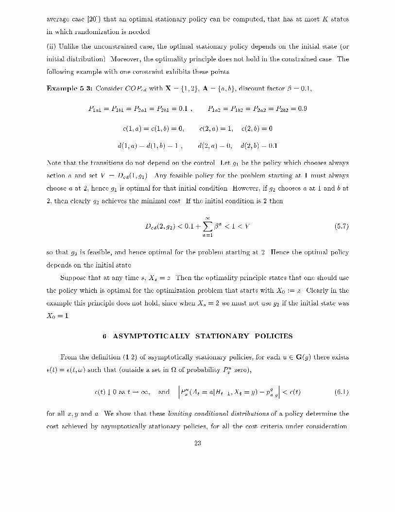
average case [20]) that an optimal stationary policy can be computed, that has at most K statesin which randomization is needed.(ii) Unlike the unconstrained case, the optimal stationary policy depends on the initial state (orinitial distribution). Moreover, the optimality principle does not hold in the constrained case. Thefollowing example with one constraint exhibits these points.Example 5.3: Consider COPed with X = f1; 2g, A = fa; bg, discount factor � = 0:1,P1a1 = P1b1 = P2a1 = P2b1 = 0:1 ; P1a2 = P1b2 = P2a2 = P2b2 = 0:9c(1; a) = c(1; b) = 0; c(2; a) = 1; c(2; b) = 0d(1; a) = d(1; b) = 1 ; d(2; a) = 0; d(2; b) = 0:1Note that the transitions do not depend on the control. Let g1 be the policy which chooses alwaysaction a and set V = Ded(1; g1). Any feasible policy for the problem starting at 1 must alwayschoose a at 2, hence g1 is optimal for that initial condition. However, if g2 chooses a at 1 and b at2, then clearly g2 achieves the minimal cost. If the initial condition is 2 thenDed(2; g2) < 0:1 + 1Xn=1�n < 1 < V (5:7)so that g2 is feasible, and hence optimal for the problem starting at 2. Hence the optimal policydepends on the initial state.Suppose that at any time s, Xs = z. Then the optimality principle states that one should usethe policy which is optimal for the optimization problem that starts with X0 := z. Clearly in theexample this principle does not hold, since when Xs = 2 we must not use g2 if the initial state wasX0 = 1. 6. ASYMPTOTICALLY STATIONARY POLICIESFrom the de�nition (1.2) of asymptotically stationary policies, for each u 2 G(g) there exists�(t) = �(t; !) such that (outside a set in of probability Pux zero),�(t) # 0 as t!1; and ���Pux (At = ajHt�1;Xt = y)� pgajy��� < �(t) (6:1)for all x; y and a. We show that these limiting conditional distributions of a policy determine thecost achieved by asymptotically stationary policies, for all the cost criteria under consideration.23

This enables the application of AS policies to the solution of all the relevant adaptive constrainedproblems.Given a policy u, denote �ux(y; a) := limt!1Pux (Xt = y;At = a) (6:2)whenever this limit exists. Note that under A1, for any stationary policy g, �gx exists and �gx(y; a) =�g(y; a) = �g(y) � g(ajy) is independent of x. The main result of this Section is that the conditionaldistributions which enter the de�nition (1.2) of an AS policy g have a role which is similar tothe conditional frequencies (3.3) in the sense that they determine the limiting probabilities (6.2)(Theorem 6.1), which in turn determine the costs (see proof of Theorem 6.4).Theorem 6.1: Under A1, given any stationary policy g, if u 2 G(g) then for any state y andinitial state x, limt!1 Pu(Xt = yjX0 = x) = �g(y), and �ux exists and is equal to �g.In order to prove Theorem 6.1 we need the following Lemma. Fix a stationary policy g and apolicy u in G(g). De�ne the matrix P (t) byfP (t)gyz := Pu(Xt = zjXt�1 = y;X0 = x) (6:3)Lemma 6.2: Assume A1 and �x some arbitrary ~� > 0, g 2 U(S) and u 2 G(g). If Pux (Xtn =y) > ~� for some increasing sequence ftng11 , then limn!1fP (tn)gyz = fP ggyz for each z.Proof of Lemma 6.2: By (6.1), for any � > 0 there exists a T� > 0 such that Pux (�(T�) > �) <�. For t > T�,jPux (At = ajXt = y)� pgajyj � ���Eux �1f�(t) � �g hPux (At = a j Ht�1;Xt = y)� pgajyi+1f�(t) > �g hPux (At = a j Ht�1;Xt = y)� pgajyi �� Xt = y����� �+ Eux�1f�(t) > �g j Xt = y� (6:4)For any tn > T�, Eux�1f�(tn) > �g j Xtn = y� � �~� . Since � is arbitrary, limn!1 Pu(Atn =ajXtn = y;X0 = x) = pgajy. The Lemma then follows by noting that Pyz(t) =Pa Pyaz �Pu(At�1 =ajXt�1 = y;X0 = x). 24

Proof of Theorem 6.1: Fix x, a and u 2 G(g). Under g, fXtg is a regular Markov chain. Hencefor some integer M (as in the proof of Lemma 4.6), [P g]M has all components nonzero (in fact itcan easily be shown that one such M is the smallest integer divisible by 2; 3; : : : ; J).Let �j be a row vector with 1 in the j-th component and 0 otherwise. Denote Qtx :=Pu(XtjX0 = x). Observe that Qtx = �x �Qts=1 P (s), where P (s) is de�ned in (6.3). This fol-lows by iteratingQtx(y) = Pu(Xt = yjX0 = x)=Xz Pu(Xt�1 = zjX0 = x) � Pu(Xt = yjXt�1 = z;X0 = x) =Xz Qt�1x (z)Puzy(t) (6:5)where the second equality is obtained from Bayes rule. In matrix notation the last equation readsQtx = Qt�1x � Pu(t). Given some ~� > 0 let P �(t) be the matrix whose elements are given byfP �(t)gyz := fP (t)gyz + fP g � P (t)gyz � 1fQt�1x (y) � ~�g (6:6)for all y; z in X. Denote R(t) := t+MYs=t+1P (t) ; R�(t) := t+MYs=t+1P �(t) (6:7)Next, we evaluate Qt+Mx �Qtx �R�(t).���Qt+1x �QtxP �(t+ 1)� (y)�� = jQt+1x (y)�Xz Qtx(z)P �zy(t+ 1)j= jXz Qtx(z)[Pzy(t+ 1)� P �zy(t+ 1)]j � ~� �M (6:8)Similarly, for an arbitrary stochastic matrix ~P ,�����Qt+1x �QtxP �(t+ 1)� ~P� (y)��� � ~� �M2 (6:9)Using (6.7)-(6.9) we obtain���Qt+Mx �QtxR�(t)� (y)�� = ���Qtx (R(t)� R�(t))� (y)�� (6:10a)� �����"QtxP (t+ 1) t+MYs=t+2P (t)� t+MYs=t+2P �(t)!# (y)�����+ �����"Qtx (P (t+ 1)� P �(t+ 1)) t+MYs=t+2P �(t)# (y)����� (6:10b)� �����"Qt+1x t+MYs=t+2P (t)� t+MYs=t+2P �(t)!# (y)�����+ ~�M2 (6:10c)25

The �rst term in (6.10c) is now handled as in (6.10a)-(6.10c), to obtain���Qt+Mx �QtxR�(t)� (y)�� � ~�M3 (6:11)Denote �1 := ~� �M4. By Lemma 6.2 and the de�nition (6.6), P �(t) converges to P g. The continuityof the mapping fP �(s)gt+Ms=t+1 ! Qt+Ms=t+1 P �(s) now implies R�(t) ! [P g]M Pux a.s. Thus thereexists some t0 such that for all t > t0, all components of R�(t) are greater than some positive �0,and �0 depends only on P g. Denote � := 1� �0.Let �t denote the stationary probability of a Markov chain whose transition probabilities aregiven by the matrix R�(t). Since all components of R�(t) are strictly positive, �t exists and isunique for all t > t0. The convergence R�(t)! [P g]M now implies (see e.g. [14]) limt!1 �t = �gsince �g is the unique invariant distribution of [P g]M . Let t1 > t0 be such that k�t� �gk1 � �1 forall t > t1. For t � t1:kQt+nMx � �gk1 � kQt+nMx � �t+(n�1)Mk1 + k�t+(n�1)M � �gk1 (6:12a)= kQt+(n�1)Mx �R(t+ (n� 1)M)� �t+(n�1)Mk1 + k�t+(n�1)M � �gk1� kQt+(n�1)Mx �R�(t+ (n� 1)M)� �t+(n�1)Mk1+ kQt+(n�1)Mx � (R(t+ (n� 1)M)� R�(t+ (n� 1)M))k1 + k�t+(n�1)M � �gk1� �kQt+(n�1)Mx � �t+(n�1)Mk1 + �1 + �1 (6:12b)where (6.12b) follows from Lemma 4.5, (6.10) and (6.11). Iterating (6.12) we obtain:kQt+nMx � �gk1 � �nkQtx � �gk1 + 2�11� � � 2�n + 2�11� � (6:13)Since ~� and hence �1 can be chosen arbitrarily small, � is independent of this choice and since �nconverges to 0, it follows that limt!1;n!1 kQt+nMx � �gk1 = 0from which it follows limt!1Pu(Xt = � jX0 = x) = limt!1Qtx = �g (6:14)This proves the �rst claim.Now observe that from (6.14), if ~� < �g(y) then Pux (Xt = y) < ~� only a �nite number of times.By A1, �g(y) > 0 for all y, so Lemma 6.2 and the argument following (6.4) imply thatlimt!1Pu(At = ajXt = y;X0 = x) = pgajy26

Since Pu(Xt = y;At = ajX0 = x) = Pu(Xt = yjX0 = x) � Pu(At = ajXt = y;X0 = x), �u existsand is equal to �g.In fact, (6.14) allows to restate Lemma 6.2 in the following stronger form.Lemma 6.20: Assume A1 and �x some g 2 U(S) and u 2 G(g). Then limt!1 P (t) = P g.Asymptotically stationary policies turn out to be a special case of ATS policies, as the nextLemma shows. Denote Ft := �fHt�1;Xtg, �x y in X and de�ne�(y;n) := the time of the nth visit strictly after 0 to state y:Lemma 6.3: Under A1, if u 2 G(g) then Fc = fpgajyg Pux a.s.Proof: Fix a and y and de�neYs := 1fXs = x;As = ag �Eux [1fXs = x;As = ag j Fs] s � 0St :=Pts=0 YsYt and St are Ft+1 measurable. Moreover, fSt;Ft+1; t � 0g is a Pux Martingale. Note that theterm in expectation in Ys can be expressed as:Eux [1fAs = a;Xs = yg j Fs] = 1fXs = yg �Eux [1fAs = ag j Fs] = 1fXs = yg � us(a j Fs)= 1fXs = yg � us(a j Hs�1;Xs = y) (6:16)Note that Ut :=Pts=0 1fXs = yg is nondecreasing, Ft measurable and, by Lemma 3.4, convergesto in�nity Pux a.s. To apply a version of the Martingale Stability Theorem [9 Theorem 2.18 p. 35],observe that by (6.16), 1Xs=0U�2s E �jYsj2 j Fs� � 1Xs=0U�2s 1fXs = yg: (6:17)With �(y;n) as in (6.15), Xt = y if and only if t = �(y;n) for some n, and U�(y;n) = n. Thus (6.17)implies 1Xs=0U�2s E �jYsj2 j Fs� � 1Xn=0n�2 <1 (6:18)27

The Martingale Stability Theorem now implies thatlimt!1 StPts=0 1fXs = yg = 0 Pux a:s:from which we obtain:limt!1 "f tc(ajy)� Pts=0 1fXs = yg � us(a j Hs�1;Xs = y)Pts=0 1fXs = yg # = 0 Pux a:s:Since limt!1 ut(a j Ht�1;Xt = y) = pgajy Pux a:s: and Pts=0 1fXs = yg ! 1 it follows thatlimt!1 f tc(ajy) = pgajy Pux a:s:which proves that Fc = fpgajyg Pux a.s.We are now in a position to prove Theorem 2.2. We show that asymptotically stationarypolicies are equivalent to the respective stationary policies, in that the costs associated with themare identical. Therefore, by Theorem 6.4, whenever g 2 U(S) is optimal under one of the costcriteria, any g 2 G(g) is optimal as well. In Section 7 we construct optimal AS policies for ACOP.Theorem 6.4: Assume A1. Then for any stationary g 2 U(S), any g 2 G(g) and any x,(i) Cea(x; g) = Cea(x; g)(ii) Cav = Cea(x; g) P gx a.s. and P gx a.s.(iii) Caed(x; g) = Caed(x; g)The results (i)-(iii) hold also for the costs associated with dk(�; �) ; k = 1; 2; : : : ;K.(iv) limN!1jCNed(x; g)� Eg[Ced(XN ; g)jX0 = x]j = 0 (6:19)limN!1jDN;ked (x; g)�Eg[Dked(XN ; g)jX0 = x]j = 0 ; 1 � k � K (6:20)Consequently, whenever g above is optimal for COPea, COPav , COPaed or COPsd, so is any g.Proof: (i) From Lemma 6.1 we have �g = �g and hencelimt!1 1t+ 1 tXs=0 Pu(Xs = y;As = a j X0 = x) = �g(y; a)28

Hence �Fsa(x; u) = f�gg = �Fsa(x; g). The result then follows from (3.1).(ii) By Lemma 6.3, Fc = fpgajyg P gx a.s. The result (ii) then follows from Lemma 3.5.(iii) Since by Lemma 6.1 �g(y; a) exists and is equal to �g(y; a), the derivation in Theorem 4.4applies verbatim to yield Caed(x; g) = [1� �]�1Cea(x; g) = Caed(x; g) : (6:21)These arguments obviously hold also for dk(�; �) ; k = 1; 2; : : : ;K.(iv) From (4.3) it follows thatEg[Ced(XN ; g)jX0 = x] = 1Xt=N �t�NXy;a Xz c(y; a)P g(Xt = y;At = ajXN = z)P g(XN = zjX0 = x)(6:22)Let uN be the policy that uses g at t � N and then uses g. ThenlimN!1 jCNed(x; g)� Eg[Ced(XN ; g)jX0 = x]j=Xy;a c(y; a)" 1Xt=N �t�N �P g(Xt = y;At = ajX0 = x)� PuN (Xt = y;At = ajX0 = x)�# (6:23)Since P g(Xt = y;At = ajX0 = x) = P g(Xt = yjX0 = x) � P g(At = ajXt = y;X0 = x) it followsby Lemma 6.1 and by de�nition of AS policies that the right hand side of (6.23) converges to zeroas N ! 1, which establishes (6.19). The argument for (6.20) is identical. The last claim of theLemma follows then from the de�nitions (2.5a-b).7. ESTIMATION AND CONTROLIn this section we introduce an optimal adaptive policy, based on \probing" and on the methodof [3]. Recall that we assume no prior information about the transition probabilities, except thatA1 holds.7.1 Estimation of the transition probabilities.De�ne P tzay := Pts=2 1fXs�1 = z;As�1 = a;Xs = ygPts=2 1fXs�1 = z;As�1 = ag29

If the denominator is zero then P t is chosen arbitrarily, but such that for every z and a, P tzay is aprobability distribution. In order thatlimt!1 P tzay = Pzay Pux a:s: (7:1)for all states z; y 2 X and a 2 A, it is su�cient that each state is visited in�nitely often andmoreover, that at each state, each action is used in�nitely often. If this condition is met, then (7.1)holds by the strong law of large numbers, as we show in (7.12){(7.13).By Lemma 3.4, each state y is indeed visited in�nitely often Pux a.s. under any policy u.By an appropriate \probing" (described below) we shall obtain P1s=2 1fXs�1 = z;As�1 = ag =1 Pux a:s: for all z 2 X; a 2 A, implying consistent estimation.The adaptive policies below de�ne actions at stopping times | when particular states arevisited. The connection between this de�nition and the de�nition of AS policies is given in thefollowing Lemma. Recall the de�nition (6.15) of �(y;n).Lemma 7.1: Assume A1. Then u 2 G(g) i� for every a; y we have Pux a:s:limn!1Pux (A�(y;n) = ajF�(y;n)) = pgajy (7:2)(�(y;n) was de�ned below Lemma 6.20).Proof: Assume u 2 G(g). Since �(y;n) � n and is �nite Pux a:s: (Lemma 3.4) we havePu(A�(y;n) = ajF�(y;n))� pgajy = 1Xt=n 1f�(y;n) = tg hPu(At = ajF�(y;n))� pgajyi (7:3)To proceed, we need to show that Pux a.s.,1f�(y;n) = tgPux (At = ajF�(y;n)) = 1f�(y;n) = tgPux (At = ajHt�1;Xt = y) (7:4)Let Y := 1fA�(y;n) = ag1f�(y;n) = tg. Clearly Eux (Y jF�(y;n)) = 1f�(y;n) = tgEux (Y jF�(y;n)), sothat for each set B 2 FtEux �1B �Eux (Y jF�(y;n))� = Eux �1B1f�(y;n) = tg � Eux (Y jF�(y;n))�= Eux �Eux (1B1f�(y;n) = tg � Y jF�(y;n))� = Eux [1B � Y ] (7:5)30

where the second equality follows since by de�nition of F�(y;n), for every Ft measurable random vari-able Z, Z �1f�(y;n) = tg is F�(y;n) measurable. By a similar argument, 1f�(y;n) = tgEux (Y jF�(y;n))is Ft measurable, so that Eux (Y jF�(y;n)) is Ft measurable and by (7.5), Eux (Y jF�(y;n)) = Eux (Y jFt).Now Eux (Y jFt) = 1f�(y;n) = tgXz Pux (At = ajHt�1;Xt = z) � 1fXt = zg= 1f�(y;n) = tgPux (At = ajHt�1;Xt = y) (7:6)which completes the proof of (7.4). Using the de�nition (6.1), equations (7.3)-(7.4) yieldPux (A�(y;n) = ajF�(y;n))� pgajy = 1Xt=n 1f�(y;n) = tg hPux (At = ajHt�1;Xt = y)� pgajyi� �(n) 1Xt=n 1f�(y;n) = tg = �(n) (7:7)and (7.2) follows.To prove the converse assume (7.2) holds. Then there exists ~�(n) = ~�(n; !) such that (outsidea set in of probability Pux zero), ~�(n) # 0 as n ! 1, and ���Pux (A�(y;n) = ajF�(y;n))� pgajy��� <~�(n) Pux a:s: Since n � �(y;n) we obtain from (7.4):Pux (At = ajHt�1;Xt = y)� pgajy = tXn=1 1f�(y;n) = tg � hPux (At = ajHt�1;Xt = y)� pgajyi= tXn=1 1f�(y;n) = tg hPux (A�(y;n) = ajF�(y;n))� pgajyi (7:8)Since �(y;n) is �nite Pux a.s., (7.2) implies for each s < tlimt!1 sXn=1 1f�(y;n) = tg hPux (A�(y;n) = ajF�(y;n))� pgajyi = 0 Pux a.s. (7:9)On the other hand,tXn=s+1 1f�(y;n) = tg hPux (A�(y;n) = ajF�(y;n))� pgajyi � ~�(s) tXn=1 1f�(y;n) = tg = ~�(s) (7:10)which can be made arbitrarily small by choosing s large enough. Combining (7.8)-(7.10), it followsthat limt!1 Pux (At = ajHt�1;Xt = y)� pgajy = 0 Pux a:s: which concludes the proof.31

7.2 The adaptive policyDe�ne B := the space of matrices f�ayg such that for each state y, f�ay ; a 2 Ag is a probabilitydistribution on A. Let g be some optimal stationary policy for COP. Let � be the stationary policyde�ned by �ajy = jAj�1 for each a; y. Fix a decreasing sequence �r # 0 such that P11 �r = 1,and an increasing sequence of times Tr with T1 = 0. Tr are the times at which we update theestimate. Suppose we are given a sequence � = f�r ; r = 1; 2; :::g where each �r 2 B depends onthe estimates of the transition probabilities Pzay; z; y 2 X; a 2 A and is an approximation of g.Such control laws are introduced in [3], and are based on sensitivity analysis of Linear Programs(e.g. [7]). In the following Algorithm we construct a policy u which is shown later to be optimalfor ACOP.Algorithm 7.2: If Xt = y and y has been visited n times, and Tr � t < Tr+1 then ut is de�nedthrough: ut(�jHt�1;Xt) = �n � �+ (1� �n) ��r(PTr) (7:11)Remark: A way to obtain each �r from the estimate PTr is given in [3], and it involves solving twoLinear Programs. One can choose Tr = q � r where q is some positive integer that is proportionalto the computation time of �r.Theorem 7.3: Assume A1 and assume that COP is feasible. Assume moreover that PTr ! Pimplies that �r(PTr) converges to g. Then the policy u obtained through Algorithm 7.2 satis�esu 2 G(g) and is optimal for ACOP.Proof: Pick some state y and an action a. By Lemma 3.4 y is visited in�nitely often Pux a.s. underany policy u. Recall the de�nition of �(y;n) in (6.15). According to (7.11) and the constructionof f�ng we have Pn!1 P (A�(y;n) = a) = 1. Hence by Borel Cantelli Lemma, at state y actiona is used in�nitely often. Let �(y; a;m) be the mth time that Xt = y;At = a. It follows that�(y; a;m) are �nite Pu a.s. since the event fXt = y;At = ag occurs i.o. Pu a.s. It can be shownthat 1fX�(y;a;m)+1 = zg; m = 1; 2; ::: are i.i.d. variables. It then follows by the Strong Law ofLarge Numbers that limm!1Pmj=1 1fX�(y;a;j)+1 = zgm = Pyaz Pu a:s: (7:12)But since Tr and �(y; a;m) are �nite Pu a.s. we havelimr!1 PTryaz = limr!1PTrt=2 1fXt�1 = y;At�1 = a;Xt = zg1fXt�1 = y;At�1 = ag =32

= limm!1Pmj=1 1fX�(y;a;j)+1 = zgm = Pyaz Pu a:s: (7:13)Since this holds for any y and a it follows that PTr ! P w.p.1. Hence by hypothesis �r(PTr)converges to g, which implies by (7.11) that Pux (A�(y;n) = ajF�(y;n)) ! pgajy. Hence u 2 G(g)is an asymptotically stationary policy by Lemma 7.1. By Theorem 6.4 it is optimal for the caseof expected average costs, average costs, asymptotic expected discounted costs, and for Sch�al'scriterion. 8. APPENDIXIn this Section we generalize Sch�al's original criterion to the constrained problem and show,using Example 5.3 that there need not exist an optimal (or even an �-optimal) policy for thisproblem.Call a policy u feasible with respect to COPSchal iflimn!1Eux " 1Xt=n �t�ndk(Xt; At)� Vk#+ = 0 k = 1; :::;Kwhere [z]+ := maxfz; 0g.Let C�ed(x) be the optimal value of COPed starting at X0 = x. A policy u is said to be optimalwith respect to COPSchal if it is feasible andlimn!1Eux ����� 1Xt=n �t�nc(Xt; At)� C�ed(Xn)����� = 0Consider Example 5.3, and note that for t � 2 we have P (Xt = 1) = 0:1 under any policy andfor any initial state. For any policy u we have:Eux " 1Xt=n �t�nd(Xt; At)� V #+ � Pux (Xn = 1)Eux 0@" 1Xt=n �t�nd(Xt; At)� V #+ ��Xn = 11A� 0:1Eux " 1Xt=n �t�nd(Xt; At)� V # ��Xn = 1!33

where the last inequality follows from Jensen's inequality and the fact that the last expression isalways non-negative. For it to converge to zero, it is clearly necessary thatlimn!1Pux (An+1 = a j Xn+1 = 2) = 1 (8:1)But note that C�(x) = 1fx = 1gC�(1) + 1fx = 2gC�(2) whereC�(1) = 1Xt=1 �0:1t � 1 � P g11 (Xt = 2)� = 0:9� 11� 0:1 � 1� = 0:1C�(2) = 0But using Jensen's inequality,Eux ����� 1Xt=n �t�nc(Xt; At)� C�ed(Xn)����� � Pux (Xn = 2)Eux ����� 1Xt=n[�t�nc(Xt; At)� C�ed(Xn)]����� jXn = 2!� Pux (Xn = 2) �����Eux " 1Xt=n �t�nc(Xt; At)� 0��Xn = 2#�����and therefore for u to be optimal it should follow asymptotically g2, i.e.limn!1Pux (An+1 = a j Xn+1 = 2) = 0which contradicts (8.1). Therefore there does not exist any optimal policy, and moreover, thereexists an � > 0 such that any feasible policy is not even �-optimal (in the obvious sense).

34

REFERENCES[1] Altman E. and A. Shwartz, \Non-stationary policies for controlled Markov Chains", June 1987,under revision.[2] Altman E. and A. Shwartz, \Markov decision problems and state-action frequencies", EE.PUB. No. 693, Technion, November 1988, under revision.[3] Altman E. and A. Shwartz, \Adaptive control of constrained Markov chains", EE. PUB. No.713, Technion, March 1989, submitted.[4] Beutler F. J. and K. W. Ross, \Optimal policies for controlled Markov chains with a con-straint", Math. Anal. Appl. Vol. 112, pp. 236-252, 1985.[5] Borkar V. S., \On minimum cost per unit time control of Markov chains", SIAM J. ControlOpt., Vol. 22 No. 6, pp. 965-978, November 1984.[6] Borkar V. S., \A convex analytic approach to Markov decision processes", Probab. Th. Rel.Fields, Vol. 78, pp. 583-602, 1988.[7] Dantzig G. B., J. Folkman and N. Shapiro, \On the continuity of the minimum set of acontinuous function", J. Math. Anal. and Applications, Vol. 17, pp. 519-548, 1967.[8] Derman C., Finite State Markovian Decision Processes, Academic Press, 1970.[9] Hall P. and C. C. Heyde, Martingale Limit Theory and its Applications, John Wiley, NewYork, 1980.[10] Hernandez-Lerma O., Adaptive Control of Markov Processes, Springer Verlag, 1989.[11] Hernandez-Lerma O. and S. I. Marcus, \Adaptive Control of Discounted Markov DecisionChains", J. Opt. Theory Appl. Vol. 46 No. 2, pp. 27-235, June 1985.[12] Hernandez-Lerma O. and S. I. Marcus, \Discretization procedures for adaptive Markov controlprocesses", J. Math. Anal . Appl., to appear.[13] Hernandez-Lerma O. and S. I. Marcus, \Adaptive policies for discrete-time stochastic systemswith unknown disturbance distribution" System Control Letters Vol. 9, pp. 307-315, 1987.[14] Hordijk A., Dynamic Programming and Markov potential theory , Mathematical Center TractsNo. 51, Amsterdam, 1974.[15] Hordijk A. and L. C. M. Kallenberg, \Constrained undiscounted stochastic dynamic program-ming", Mathematics of Operations Research, Vol. 9, No. 2, May 1984.[16] Kallenberg L. C. M., Linear Programming and Finite Markovian Control Problems, Math.Centre Tracts 148, Amsterdam, 1983.[17] Kemeny J. G. and J. L. Snell, Finite Markov Chains , D. Van Nostrand Company, 1960.35

[18] Kumar P. R., \A survey of some results in stochastic adaptive control", SIAM J. Control Opt.,Vol. 23 No. 3, pp. 329-380, May 1985.[19] Makowski A. M. and A. Shwartz, \Implementation issues for Markov decision processes", Proc.of a workshop on Stochastic Di�erential Systems, Stochastic Control Theory and Applications,Inst. Math. Appl., Univ. of Minnesota, Springer-Verlag Lecture Notes, Control and Inf. Sci.,Edited by W. Fleming and P.-L. Lions, 1986.[20] Ross K. W., \Randomized and past-dependent policies for Markov decision processes withmultiple constraints", Operations Research, Vol. 37, No. 3, May 1989.[21] Ross K. W. and A R. Varadarajan, \Markov decision processes with sample path constraints:Unichain, communicating and deterministic cases", Submitted to Operations Research, July1986.[22] Sch�al M., \Conditions for optimality in dynamic programming and for the limit of n-stageoptimal policies to be optimal", Z. Wahrscheinlichkeitstheorie und verw. Geb. Vol. 32, pp.179-196, 1975.[23] Sch�al M., \Estimation and control in discounted dynamic programming," Stochastics 20, pp.51-71, 1987.[24] Shwartz A. and A. M. Makowski, \An Optimal Adaptive Scheme for Two Competing Queueswith Constraints", Analysis and Opt. of Systems, edited by A. Bensoussan and J. L. Lions,Springer Verlag lecture notes in Control and Info. Scie. No. 83, 1986.[25] Van Hee, K. M. Bayesian Control of Markov Chains, Mathematical Centre Tracts 95, Ams-terdam, 1978.

36