Activated Region Fitting: A Robust High-PowerMethod for fMRI Analysis Using Parameterized

Regions of Activation

Wouter D. Weeda,1* Lourens J. Waldorp,1 Ingrid Christoffels,2,3

and Hilde M. Huizenga1

1Department of Psychology, University of Amsterdam, Amsterdam, The Netherlands2Leiden Institute for Psychological Research, Leiden University, Leiden, The Netherlands3Leiden Institute for Brain and Cognition, Leiden University, Leiden, The Netherlands

Abstract: An important issue in the analysis of fMRI is how to account for the spatial smoothness ofactivated regions. In this article a method is proposed to accomplish this by modeling activated regionswith Gaussian shapes. Hypothesis tests on the location, spatial extent, and amplitude of these regionsare performed instead of hypothesis tests of individual voxels. This increases power and eases interpre-tation. Simulation studies show robust hypothesis tests under misspecification of the shape model, andincreased power over standard techniques especially at low signal-to-noise ratios. An application toreal single-subject data also indicates that the method has increased power over standard methods.Hum Brain Mapp 00:000–000, 2009. VVC 2009 Wiley-Liss, Inc.

Key words: spatial model; voxel correlations; robust inference; false discovery rate; cluster size thresh-old; sandwich estimation

INTRODUCTION

The main purpose of fMRI analysis is to determinewhich brain regions are activated. This question isanswered by looking for groups of significantly activatedvoxels but not by looking for single voxel activity. At thebasis of this train of thought is the assumption that activa-tion (i.e. the BOLD response) measured by fMRI has a spa-tial extent of several millimeters and that the activation

pattern is smooth [Hartvig, 2002]. This assumption is oftenincorporated by assuming positive spatial correlationsbetween voxels, either positive correlations between fMRInoise or positive correlations between fMRI signals. Meth-ods that incorporate fMRI noise correlations are, for exam-ple, Monte Carlo multiple testing corrections [Formanet al., 1995], permutation test frameworks [Hayasaka andNichols, 2004], preprocessing smoothing kernels [Frimanet al., 2003], and random field theory [Poline et al., 1997;Worsley et al., 1996]. Methods that incorporate signal cor-relations are clustering approaches [Neumann et al., 2006;Thirion et al., 2006], spatiotemporal analyses [Bowman,2005; Kiebel et al., 2000], mixture models with spatial con-straints [Hartvig and Jensen, 2000; Woolrich et al., 2005],and priors in a Bayesian framework [Flandin and Penny,2007; Penny and Friston, 2003].Another way to incorporate positive spatial correlations

of fMRI signals is to explicitly use the assumptions of anunderlying smooth process to model the spatial activationpattern. By assuming that each active brain region can be

Contract grant sponsor: Netherlands’ Organization for ScientificResearch (NWO).

*Correspondence to: Wouter D. Weeda, Department of Psychol-ogy, University of Amsterdam, Roetersstraat 15, 1018 WB Amster-dam, The Netherlands. E-mail: w.d.weeda1@uva.nl

Received for publication 2 October 2007; Revised 2 October 2008;Accepted 10 October 2008

DOI: 10.1002/hbm.20697Published online in Wiley InterScience (www.interscience.wiley.com).

VVC 2009 Wiley-Liss, Inc.

r Human Brain Mapping 00:000–000 (2009) r

approximated by a generic spatial model of activation, onecan model activity in an entire fMRI image [Hartvig, 2002;Lukic et al. 2004, 2007; Tzikas et al., 2004]. The successful-ness of this type of method depends on the shape modelused. A model too simple leads to severe misspecificationand biased inference. A model too complex may describethe shape of activation well but may hinder interpretation,because of modeling noise and containing too many pa-rameters.Aiming for a sensible, easy to interpret way to analyze

the spatial pattern of fMRI data we propose an alternativemethod of fMRI analysis, termed ‘‘activated region fitting’’(ARF). At the heart lies the assumption that a region ofbrain activation can be approximated by a Gaussian-shaped function and that a number of these Gaussianfunctions can be used to describe the activation pattern inan fMRI image. The Gaussian function was chosen as it isrelatively simple—it uses six parameters which are easy tointerpret—and still has good flexibility in terms of differ-ent shapes. The optimal number of Gaussians is deter-mined by fitting increasingly complex models (i.e. moreGaussian functions) to the data until a parsimoniousdescription of the data is given. Hypothesis tests are thenperformed on the parameters of the Gaussian functions,allowing for hypotheses of location, spatial extent, and am-plitude.Analyzing fMRI data with ARF has several advantages.

First, an objective measure is available for the location,spatial extent, and amplitude of each area of activation.Second, these locations, spatial extents, and amplitudesmay serve as input for a functional connectivity analysis.Third, an entire image is described with relatively few pa-rameters, thereby increasing power and reducing the mul-tiple testing problem. Fourth, ARF corrects for model mis-specification, allowing for robust hypothesis tests. Fifth, asthe method of ARF is performed on the output of a stand-ard GLM analysis (unthresholded), it is easy to add to thestandard analysis steps and computational load is rela-tively low.The outline of the article is as follows. First, the techni-

cal details of ARF will be explained. Details on the spa-tial model, parameter and variance estimation, model fit,and hypothesis testing will be given. Thereafter, detailson the simulation studies are given, performed to assessbias, variance estimation under misspecification, andpower. Then an application to real data is given, fol-lowed by the discussion in which the findings are sum-marized, and in which possible limitations and exten-sions are highlighted.

METHOD

ARF works by fitting a spatial model of activation to anentire image of signal change. This image is either a 2Dslice or a flattened 3D map. The spatial model is one, or asum of two or more bivariate Gaussian-shaped regions.

Each region is described by two parameters to model thelocation of activation, three parameters to model the extentof activation, and one parameter to model the amplitudeof activation. The spatial model is fitted to the data usinggeneralized least squares (GLS). The number of regionsthat best describe the data is decided by using the Bayes-ian information criterion (BIC). Once a decision is made onthe number of regions, robust hypothesis tests are per-formed on the parameters of the regions. The followingsections will explain the ARF method in detail.

Input

ARF works on the estimated scaling parameters andassociated variances of a standard GLM analysis (note thatt-values can also be used, with their variances set to 1).ARF requires multiple independent measurements of thecondition of interest. This requires multiple measurementsfrom different runs of the experiment. In a block designthe multiple measurements can be derived from multipleblocks of the same condition. In an event-related designthe data of several runs of the experiment can be used. AGLM analysis is performed on these multiple measure-ments, and the resulting unthresholded values are thenused as trials in the ARF analysis. The number of trials inthe present study was set to either 5 or 15, but other val-ues can be chosen as well. The actual ARF estimation isperformed on the average over these trials. The individualtrials are used to obtain robust hypothesis tests.Let bk be a (N 3 1) vector, with N indicating the num-

ber of voxels, containing the scaling parameters from theGLM analysis of trial k. Let rk

2 be a (N 3 1) vector con-taining the squared standard errors of bk. The averageover K trials is then:

b ¼ 1

K

XKk¼1

bk ð1Þ

Assuming independent variances rk2 over k 5 1, . . . , K

trials, the variance of b is calculated as follows [Parzen,1960]:

w¼ 1

K2

XKk¼1

r2k ð2Þ

with w being a (N 3 1) vector of variances.

Spatial Model

The main assumption in the ARF procedure is the spa-tial model used to describe the data. This shape modelmust be anatomically sensible, relatively simple, and inter-pretable. For these reasons a slight adaptation of a bivari-ate Gaussian distribution function was chosen. A graphicalrepresentation of a region is given in Figure 1.

r Weeda et al. r

r 2 r

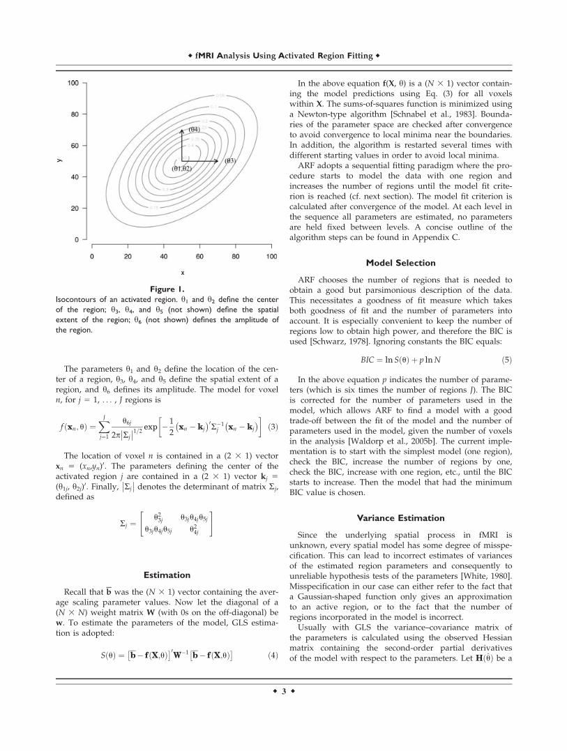
The parameters y1 and y2 define the location of the cen-ter of a region, y3, y4, and y5 define the spatial extent of aregion, and y6 defines its amplitude. The model for voxeln, for j 5 1, . . . , J regions is

f xn; uð Þ ¼XJ

j¼1

u6j

2p Rj

�� ��1=2 exp � 1

2xn � kj

� �0R�1j xn � kj

� �� �ð3Þ

The location of voxel n is contained in a (2 3 1) vectorxn 5 (xn,yn)

0. The parameters defining the center of theactivated region j are contained in a (2 3 1) vector kj 5(y1j, y2j)0. Finally, Rj

�� �� denotes the determinant of matrix Sj,defined as

Rj ¼u23j u3ju4ju5j

u3ju4ju5j u24j

" #

Estimation

Recall that b was the (N 3 1) vector containing the aver-age scaling parameter values. Now let the diagonal of a(N 3 N) weight matrix W (with 0s on the off-diagonal) bew. To estimate the parameters of the model, GLS estima-tion is adopted:

S uð Þ ¼ b� f X;uð Þ� �0W�1 b� f X;uð Þ� � ð4Þ

In the above equation f(X, y) is a (N 3 1) vector contain-ing the model predictions using Eq. (3) for all voxelswithin X. The sums-of-squares function is minimized usinga Newton-type algorithm [Schnabel et al., 1983]. Bounda-ries of the parameter space are checked after convergenceto avoid convergence to local minima near the boundaries.In addition, the algorithm is restarted several times withdifferent starting values in order to avoid local minima.ARF adopts a sequential fitting paradigm where the pro-

cedure starts to model the data with one region andincreases the number of regions until the model fit crite-rion is reached (cf. next section). The model fit criterion iscalculated after convergence of the model. At each level inthe sequence all parameters are estimated, no parametersare held fixed between levels. A concise outline of thealgorithm steps can be found in Appendix C.

Model Selection

ARF chooses the number of regions that is needed toobtain a good but parsimonious description of the data.This necessitates a goodness of fit measure which takesboth goodness of fit and the number of parameters intoaccount. It is especially convenient to keep the number ofregions low to obtain high power, and therefore the BIC isused [Schwarz, 1978]. Ignoring constants the BIC equals:

BIC ¼ ln S uð Þ þ p lnN ð5Þ

In the above equation p indicates the number of parame-ters (which is six times the number of regions J). The BICis corrected for the number of parameters used in themodel, which allows ARF to find a model with a goodtrade-off between the fit of the model and the number ofparameters used in the model, given the number of voxelsin the analysis [Waldorp et al., 2005b]. The current imple-mentation is to start with the simplest model (one region),check the BIC, increase the number of regions by one,check the BIC, increase with one region, etc., until the BICstarts to increase. Then the model that had the minimumBIC value is chosen.

Variance Estimation

Since the underlying spatial process in fMRI isunknown, every spatial model has some degree of misspe-cification. This can lead to incorrect estimates of variancesof the estimated region parameters and consequently tounreliable hypothesis tests of the parameters [White, 1980].Misspecification in our case can either refer to the fact thata Gaussian-shaped function only gives an approximationto an active region, or to the fact that the number ofregions incorporated in the model is incorrect.Usually with GLS the variance–covariance matrix of

the parameters is calculated using the observed Hessianmatrix containing the second-order partial derivativesof the model with respect to the parameters. Let HðuÞ be a

Figure 1.

Isocontours of an activated region. y1 and y2 define the center

of the region; y3, y4, and y5 (not shown) define the spatial

extent of the region; y6 (not shown) defines the amplitude of

the region.

r fMRI Analysis Using Activated Region Fitting r

r 3 r

(p 3 p) matrix, such that each element (r 5 1, . . . , p; s 5 1,. . . , p):

hrs u� � ¼ XN

n¼1

1

wn

@fn uð Þ@ur

@fn uð Þ@us

� �bn � fn uð Þ� � @2fn uð Þ@ur@us

� u¼u

� �

ð6Þ

[Seber and Wild, 1989]. The variance–covariance matrixCðuÞ is then calculated by:

C u� � ¼ S u

� �N � pð Þ H u

� �� ��1 ð7Þ

Equations (6) and (7) assume that the model is correctlyspecified [Waldorp et al., 2005a; White, 1980], an assump-tion that is not tenable in the situation of ARF. To correctfor this misspecification the variances of the parameterestimates are calculated using the sandwich estimate [Wal-dorp et al., 2005a; White, 1980]. Let FðuÞ be the (N 3 p)matrix of first-order derivatives of the model with respectto the parameters. Let RðuÞ be a (N 3 N) matrix of the out-erproduct of the residuals:

R u� � ¼ 1

K2

XKk¼1

bk � f u� �� �

bk � f u� �� �0 ð8Þ

Note that each element in RðuÞ has to be divided by thenumber of trials once more to scale it to the averaged data.The sandwich estimate is then as follows:

C u� � ¼ S u

� �N � pð Þ H u

� �� ��1F u� �0

W�1R u� �

W�1F u� �

H u� �� ��1

ð9Þ

Note in addition that when the model is correctly speci-fied in both the mean and variance, the function reverts tothe standard expression for the covariance matrix of pa-rameters estimates [cf. Seber and Wild, 1989, paragraph12.2.4], as the matrix RðuÞ containing the residuals, goes toW and the residuals in HðuÞ tend to zero. For spatiallyuncorrelated data the diagonal of RðuÞ can be used.

Hypothesis Testing

ARF allows hypothesis tests on the parameters of eachactivated region, or on functions of these parameters. Hy-pothesis tests on the location, spatial extent, and amplitudeof the regions can be performed, individually and as anomnibus test. All tests are calculated by a Wald statistic[Seber and Wild, 1989] and are calculated for each acti-vated region j. That is, the hypothesis tests are calculatedper region. The test statistic equals:

a0 uj� �h

AjCjA0j

i�1

a uj� � ð10Þ

In the above equation Cj denotes the (6 3 6) variance–covariance matrix of the parameter estimates of a region j.aðujÞ is a (4 3 1) column vector which consists of fournull-hypotheses, namely, (1) the x-coordinate of the centerof region j equals a hypothesized x-coordinate c1, (2) the y-coordinate of the center of region j equals a hypothesizedy-coordinate c2, (3) the spatial extent of region j is 0, and(4) the amplitude of region j is 0. Note that the extent of aregion can be defined by the determinant of matrix S fromEq. (3), where this determinant is given by the usual

expression for a 2 3 2 matrix deta bc d

� � �¼ ad� bc

[Schott, 1997]. So a0 uj� �

is defined as follows:

a0 uj� � ¼ u1j � c1

x locationu2j � c2

y locationu23ju

24j � u23ju

24ju

25j

extent

u6jamplitude

� �ð11Þ

Aj is defined as a (4 3 6) matrix containing the partial

derivatives of aðujÞ to the yj-parameters:

Aj ¼

1 0 0 0

0 1 0 0

0 0 2u3ju24j 1� u25j

� � 2u4ju

23j 1� u25j

� � 0 0 0 0

266664

0 0

0 0

�2u5ju23ju

24j

� 0

0 1

377775 ð12Þ

The test-statistic in Eq. (10) under H0 is asymptotically Fdistributed with N and (N 2 p) degrees of freedom [Seberand Wild, 1989; for misspecified models, see White, 1982],with p indicating the number of parameters.The Wald statistic is based on the estimated variances of

parameter estimates, and these variances are only estimatedadequately in asymptotic circumstances, in our case, if thenumber of voxels is very large and/or if the signal-to-noiseratio (SNR) is high [cf. Seber and Wild, 1989]. In nonasymp-totic cases the variances might be underestimated thus giv-ing rise to tests that are too liberal [see, for example, Fears,1996; Seber and Wild, 1989]. Therefore we determined insimulations whether the variances are estimated adequately.If so, then the asymptotic approximation is adequate andthe test results can be trusted.

Starting Values

Starting values might be calculated by searching formaxima in the input map. The x and y location of a maxi-mum are used as the starting values for y1j and y2j. At thislocation the starting values for y3j and y4j are calculated byfinding at what distance from this maximum the input val-ues are half this maximum. The starting values of y5j and

r Weeda et al. r

r 4 r

y6j are manually set. To overcome problems with conver-gence to local minima, the procedure can be run severaltimes with different starting values.

Simulations

To check the ARF procedure several simulation studieswere performed. First, the procedure was checked for pro-ducing unbiased parameter estimates, i.e. it was deter-mined if the simulation parameters were correctly recov-ered by the procedure. Second, the variance estimates ofthe parameters were checked to be adequate and robustagainst model misspecification in different SNR conditions.Finally, the procedure was tested for its detection powerin different SNR conditions.For the simulation studies, maps with 18 3 18 voxels

were created. The signals were either the correct model, amisspecified model in shape, or a misspecified model inthe number of regions. Different SNRs were created byadjusting the amount of noise added to the signals. Thechosen SNR values were calculated over the image mapand were set at 1, 2, 5, and 10 [Smith and Nichols,2009], with SNR 1 and 2 indicating low SNRs and 5 and10 indicating high SNRs. In Appendix A the setting ofSNRs is explained in more detail. The number of trialswas set to either 5 or 15, but the SNR of the averaged datawas held constant between these two trial conditions. Toget an adequate measure of parameter recovery, varianceestimates, and detection power, each condition was run1,000 times.

Correct model

The correct spatial model used the Gaussian model asspecified in Eq. (3). For the simulations the following pa-rameters were used, y 5 (9,9,2,3,0.1,100)0, creating aslightly rotated elliptical activation area. The simulationswere used to check correct parameter recovery, to checkthe variance estimates, and to perform power analyses.

Incorrect shape model

The shape model in this case was a pyramidal shape,with a base of 7 3 5 voxels, placed in the center of themap. The data were not smoothed, thus creating a misspe-cified shape. This model was used to check the varianceestimates and to perform power analyses.

Incorrect number of regions

The shape model in this case was the sum of two Gaus-sian regions placed next to each other in the map usingthe following parameters: y1 5 (8,8,1,220.3,50)0, y2 5(10,10,1,3,0.3,70)0. The ARF procedure was set to fit onlyone region, therefore creating a model misspecified in thenumber of regions. This model was used to check the var-iance estimates and to perform power analyses.

Standard thresholding

To compare ARF with standard voxel-wise thresholdmethods, Bonferroni, false discovery rate (FDR) [Genoveseet al., 2002; Nichols and Hayasaka, 2003], and the cluster-size threshold corrections [Forman et al., 1995] were cho-sen. For FDR the q parameter was set to 0.05 and the C pa-rameter was set to 1, which are common values in fMRIstudies [Genovese et al., 2002]. The cluster-size thresholdwas determined using the Bonferroni corrected P-valueand a cluster size of 3 contiguous voxels.

RESULTS

Parameter Recovery

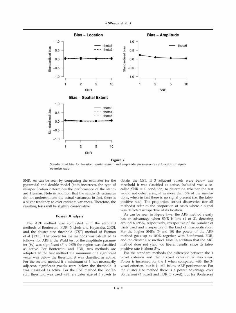
Bias in parameter estimates was calculated for each pa-rameter at different SNR values. The bias was divided byits standard error to obtain standardized bias.As can be seen in Figure 2, the bias is approximately

zero. The parameters are recovered successfully with highaccuracy even in low SNR conditions.

Variance Estimation

To evaluate the ARF procedure in producing correct var-iance estimates, the correct model, the pyramidal modeland the ‘‘incorrect number of regions model’’ (doublemodel) were used to create data that were subsequentlyanalyzed with a model with one Gaussian shape. The var-iance estimation was performed using Eq. (9) with a diago-nal RðuÞ matrix and differing numbers of trials (5 and 15).The sandwich estimations were furthermore contrastedwith standard variance estimation based on the standardHessian matrix using Eq. (7). It is expected that the sand-wich estimates will outperform the standard estimates.To promote conciseness, only the results for the location

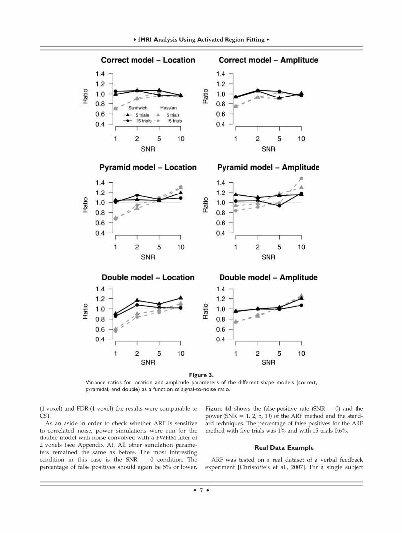
and amplitude parameters will be reported. For these pa-rameters the mean estimated variances over the 1,000 sim-ulations were divided by the variance of the parameterestimates over the 1,000 simulations. This ratio should beclose to 1. Ratios higher than 1 indicate too large estimatedvariances and thus conservativeness of the ARF procedure;whereas ratios lower than 1 would indicate liberal testing.Figure 3 shows the variance ratios for the three different

models. As can be seen the sandwich estimates performbetter than the standard Hessian estimates in all situations.For the correct model, the sandwich estimates are to bepreferred in low SNR conditions and are equal to the Hes-sian estimates for the higher SNR conditions. For the incor-rect models, the sandwich estimates are in all SNR condi-tions more adequate than the Hessian estimates. It can alsobe seen that the number of trials used for the sandwichestimation does not have a profound effect on the ratios,thus indicating that only five trials are sufficient. Note thatthe estimates of the standard Hessian for misspecifiedmodels are too small for low SNR and too large for high

r fMRI Analysis Using Activated Region Fitting r

r 5 r

SNR. As can be seen by comparing the estimates for thepyramidal and double model (both incorrect), the type ofmisspecification determines the performance of the stand-ard Hessian. Note in addition that the sandwich estimatesdo not underestimate the actual variances; in fact, there isa slight tendency to over estimate variances. Therefore, theresulting tests will be slightly conservative.

Power Analysis

The ARF method was contrasted with the standardmethods of Bonferroni, FDR [Nichols and Hayasaka, 2003],and the cluster size threshold (CST) method of Formanet al. [1995]. The power for the methods was calculated asfollows: for ARF if the Wald test of the amplitude parame-ter ðu6Þ was significant (P < 0.05) the region was classifiedas active. For Bonferroni and FDR, two methods areadopted. In the first method if a minimum of 1 significantvoxel was below the threshold it was classified as active.For the second method if a minimum of 3, not necessarilyadjacent, significant voxels were below the threshold itwas classified as active. For the CST method the Bonfer-roni threshold was used with a cluster size of 3 voxels to

obtain the CST. If 3 adjacent voxels were below thisthreshold it was classified as active. Included was a so-called SNR 5 0 condition, to determine whether the testwould not detect a signal in more than 5% of the simula-tions, when in fact there is no signal present (i.e. the false-positive rate). The proportion correct discoveries (for allmethods) refer to the proportion of cases where a signalwas detected irrespective of its location.As can be seen in Figure 4a–c, the ARF method clearly

has an advantage when SNR is low (1 or 2), detectingaround 60–95%, respectively, irrespective of the number oftrials used and irrespective of the kind of misspecification.For the higher SNRs (5 and 10) the power of the ARFmethod goes up to 100% together with Bonferroni, FDR,and the cluster size method. Note in addition that the ARFmethod does not yield too liberal results, since its false-positive rate is about 5%.For the standard methods the difference between the 1

voxel criterion and the 3 voxel criterion is also clear.Power is increased for the 1 when compared with the 3-voxel criterion, but it is still below ARF performance. Forthe cluster size method there is a power advantage overBonferroni (3 voxel) and FDR (3 voxel). But for Bonferroni

Figure 2.

Standardized bias for location, spatial extent, and amplitude parameters as a function of signal-

to-noise ratio.

r Weeda et al. r

r 6 r

(1 voxel) and FDR (1 voxel) the results were comparable toCST.As an aside in order to check whether ARF is sensitive

to correlated noise, power simulations were run for thedouble model with noise convolved with a FWHM filter of2 voxels (see Appendix A). All other simulation parame-ters remained the same as before. The most interestingcondition in this case is the SNR 5 0 condition. Thepercentage of false positives should again be 5% or lower.

Figure 4d shows the false-positive rate (SNR 5 0) and thepower (SNR 5 1, 2, 5, 10) of the ARF method and the stand-ard techniques. The percentage of false positives for the ARFmethod with five trials was 1% and with 15 trials 0.6%.

Real Data Example

ARF was tested on a real dataset of a verbal feedbackexperiment [Christoffels et al., 2007]. For a single subject

Figure 3.

Variance ratios for location and amplitude parameters of the different shape models (correct,

pyramidal, and double) as a function of signal-to-noise ratio.

r fMRI Analysis Using Activated Region Fitting r

r 7 r

an inflated brain was created for the left hemisphere. Forfour runs the unthresholded t-values (df 5 133), includingnegative values, were exported as four trials analyzed byARF. The images consisted of 126 3 74 voxels and wereaveraged over trials, creating the average map to estimatethe ARF regions. The distribution of the averaged t-valueshad a minimum of 24.22, a mean of 0.12, and a maximumof 4.28. The first quartile was 20.64 and the third quartilewas 0.98. This created a highly peaked and small taileddistribution. The input image is shown in Figure 5.

Standard thresholding with a FDR correction yieldedonly 2 significant voxels (mainly because the small tails ofthe distribution), and both CST (with Bonferroni thresholdand a cluster size of 3 voxels) and Bonferroni showed nosignificant voxels. The significant FDR voxels are markedin black in Figure 5. For the ARF procedure a sequentialfitting of 18 regions was performed to select the correctmodel. The program was run in R [R Development CoreTeam, 2007] and took 37.5 min for the final solution on a2.21-GHz AMD Opteron. The ARF algorithms are available

Figure 4.

Proportion correct discoveries (power) for activated region fitting, Cluster size threshold, false

discovery rate, and Bonferroni as a function of signal-to-noise ratio for three shape models

[correct (a), pyramidal (b), and double (c)]. (a–c) The uncorrelated noise data. (d) The corre-

lated noise data with the double model. [Color figure can be viewed in the online issue, which

is available at www.interscience.wiley.com.]

r Weeda et al. r

r 8 r

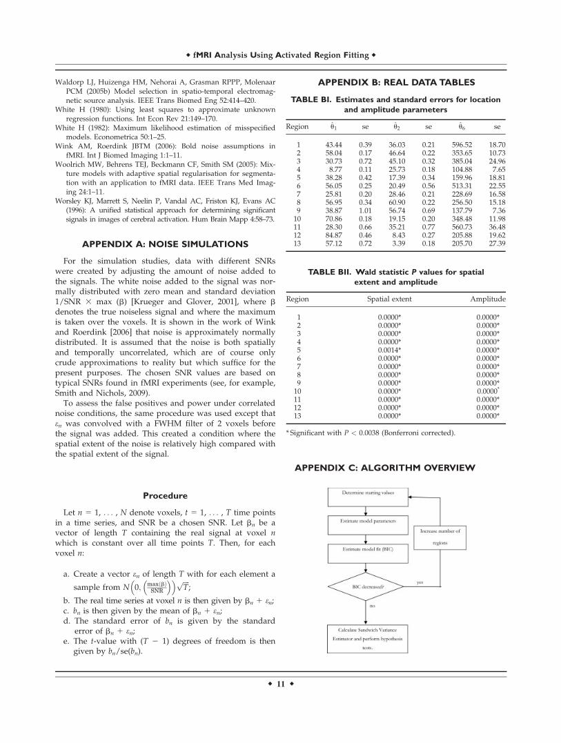
as a free R package and can be downloaded from (http://home.medewerker.uva.nl/w.d.weeda1/). The BIC indi-cated that a model with 13 regions showed the best fit, ascan be seen in Figure 6. The variances of the region param-eters were derived from the sandwich estimates. Details ofthe estimates and test are shown in Tables BI and BII (Ap-pendix B). The final solution is displayed in Figure 7.The ARF solution clearly yields more significant active

regions than the standard thresholded image, again show-ing increased power over standard techniques. Note that

these results were obtained for a single subject. It may alsobe clear that with 4 [location (2), spatial extent (1) and am-plitude (1)] 3 13 5 52 parameters of interest, the ARF so-lution gives a very concise description of the 126 3 74 59,324 voxels.

DISCUSSION

The method of ARF uses the observation that fMRI acti-vation consists of spatially smooth clusters: it describes anentire fMRI image with a multitude of Gaussian-shapedregions. In the simulations and in a real experiment it wasshown that ARF is robust against model misspecificationand has increased detection power over standard thresh-olding techniques. Although ARF has increased power, itwas also shown that ARF does yield tests that are slightlyconservative. This indicates that the regions detected byARF can be considered as being active regions, but theremay still be other active regions that remain undetected.Three extensions of ARF might be considered. First, ARF

works on 2D slices or flattened 3D images. The methodmay be extended to 3D. This requires however one addi-tional parameter to define location, and three additionalparameters to define the spatial extent of each activatedregion. This increases computational complexity and mightreduce the power of the technique. This added to the factthat fMRI results are nearly always presented in 2D, sug-gesting that the 2D or flattened 3D analysis might suffice.Second, in our simulations we have assumed that the

temporal noise is uncorrelated. Of course this is an unreal-istic assumption, but in real applications an appropriatetemporal correlation model can be incorporated in theGLM that serves as input for the ARF procedure. Third,although we showed in simulations that ARF does notdetect any spurious clusters introduced by correlated

Figure 5.

Average activation (t-values) of the left hemisphere from four runs

of the experiment (unthresholded). Active voxels (based on FDR

correction) are marked black. [Color figure can be viewed in the

online issue, which is available at www.interscience.wiley.com.]

Figure 6.

BIC values for 18 sequential models. The triangle indicates the

best fitting model (13 regions).

Figure 7.

Activated region fitting solution with 13 active regions. [Color

figure can be viewed in the online issue, which is available at

www.interscience.wiley.com.]

r fMRI Analysis Using Activated Region Fitting r

r 9 r

noise, the performance of ARF in such situations shouldbe studied further.The idea of using specific shape models is not entirely

new to fMRI analysis. One of the most well-known imple-mentations comes from Hartvig [2002], who also uses aGaussian shape model to describe regions of fMRI images.The main difference between the Stochastic GeometryModel of Hartvig and ARF is that the former is a spatio-temporal approach in a Bayesian framework, while ARFuses temporal and spatial information in distinct models.Therefore, ARF might be more applicable in practice,because standard analysis packages can be used to pre-process and analyze the temporal structure, after whichARF is invoked to model the spatial structure.Lukic et al. [2007] also used an explicit shape model to

describe fMRI data very similar to the ARF method. Bothmethods fit a multitude of spatial functions to activationdata and use the parameters to test hypotheses. The majordifference between the methods is that ARF uses a Gaus-sian shape with parameter estimates of location, spatialextent, and amplitude, whereas in the method of Lukicet al. a blurred pillbox shape or a Gaussian shape with afixed width was used. In this sense ARF has more flexibil-ity in shapes of activation. Another advantage of ARF isthat it produces robust hypothesis tests under misspecifica-tion of the shape model.In sum, it is important to account for the spatial smooth-

ness of activated regions, since it improves the detectionpower. ARF accounts for spatial smoothness by parameter-izing activated regions by Gaussian shapes. Since this onlygives an approximation to reality, the tests on region pa-rameters are designed to be robust against model specifica-tion. Simulation studies and a real data example haveshown that ARF is a robust high-power method for fMRIanalysis.

ACKNOWLEDGMENTS

The authors thank three anonymous referees for theirvaluable comments.

REFERENCES

Bowman FD (2005): Spatio-temporal modeling of localized brainactivity. Biostatistics 6:558–575.

Christoffels IK, Formisano E, Schiller NO (2007): Neural correlatesof verbal feedback processing: An fMRI study employing overtspeech. Hum Brain Mapp 28:868–879.

Fears TR, Benichou J, Gail MH (1996): A reminder of the fallibilityof the Wald statistic. Am Stat 50:225–226.

Flandin G, Penny W (2007): Bayesian fMRI data analysis withsparse spatial basis function priors. Neuroimage 34:1108–1125.

Forman SD, Cohen JD, Fitzgerald M, Eddy WF, Mintum MA, NollDC (1995): Improved assessment of significant activation infunctional magnetic resonance imaging (fMRI): Use of a clus-ter-size threshold. Magn Reson Med 33:636–647.

Friman O, Borga M, Lundberg P, Knutsson H (2003): Adaptiveanalysis of fMRI data. Neuroimage 19:837–845.

Genovese CR, Lazar N, Nichols TE (2002): Thresholding of statisti-cal maps in functional neuroimaging using the false discoveryrate. Neuroimage 15:870–878.

Hartvig NV (2002): A stochastic geometry model for functionalmagnetic resonance images. Scand J Stat 29:333–353.

Hartvig NV, Jensen JL (2000): Spatial mixture modeling of fMRIdata. Hum Brain Mapp 11:233–248.

Hayasaka S, Nichols TE (2004): Combining voxel intensity andcluster extent with permutation test framework. Neuroimage23:54–63.

Kiebel SJ, Goebel R, Friston KJ (2000): Anatomically informed ba-sis functions. Neuroimage 11:656–667.

Krueger G, Glover GH (2001): Physiological noise in oxygenation-sensitive magnetic resonance imaging. Magn Reson Med 46:631–637.

Lukic AS, Wernick MN, Galatsanos NP, Yang Y, Strother SC(2004): Reversible jump Markov chain Monte Carlo signaldetection in functional neuroimaging analysis. In: Proceedingsof the IEEE International Symposium on Biomedical Imaging1:868–871.

Lukic AS, Wernick MN, Tzikas DG, Chen X, Likas A, GalatsanosNP, Yang Y, Zhao F, Strother SC (2007): Bayesian kernel meth-ods for analysis of functional neuroimages. IEEE Trans MedImaging 26:1613–1624.

Neumann J, von Cramon DY, Forstmann BU, Zysset S, LohmannG (2006): The parcellation of cortical areas using replicator dy-namics in fMRI. Neuroimage 23:208–219.

Nichols TE, Hayasaka S (2003): Controlling the familywise errorrate in functional neuroimaging: A comparative review. StatMethods Med Res 12:419–446.

Parzen E (1960): Modern Probability Theory and Its Applications.New York: Wiley.

Penny W, Friston KJ (2003): Mixtures of general linear models forfunctional neuroimaging. IEEE Trans Med Imaging 22:504–514.

Poline JB, Worsley KJ, Evans AC, Friston KJ (1997): Combiningspatial extent and peak intensity to test for activations in func-tional imaging. Neuroimage 5:83–96.

R Development Core Team (2007): R: A language and environ-ment for statistical computing. R Foundation for StatisticalComputing, Vienna, Austria. Available at www.R-project.org.ISBN 3-900051-07-0.

Schnabel RB, Koontz JE, Weiss BE (1983): A modular system ofalgorithms for unconstrained minimization. ACM Trans MathSoftware 11:419–440.

Schott JR (1997): Matrix Analysis for Statistics. New York: Wiley.Schwarz G (1978): Estimating the dimension of a model. Ann Stat

6:461–464.Seber GAF, Wild CJ (1989): Nonlinear Regression. New York: Wiley.

Smith SM, Nichols TE (2009): Threshold-free cluster enhancement:

Addressing problems of smoothing, threshold dependence and

localization in cluster inference. Neuroimage 44:83–98.

Thirion B, Flandin G, Pinel P, Roche A, Ciuciu P, Poline JB (2006):

Dealing with the shortcomings of spatial normalization: multi-

subject parcellation of fMRI datasets. Hum Brain Mapp 27:678–

693.Tzikas DG, Likas A, Galatsanos NP, Lukic AS, Wernick MN

(2004): Relevance vector machine analysis of functional neuroi-mages. In: Proceedings of the IEEE International Symposiumon Biomedical Imaging. pp 1004–1007.

Waldorp LJ, Huizenga HM, Grasman RPPP (2005a) The Wald

test and Cramer-Rao bound for misspecified models in elec-

tromagnetic source analysis. IEEE Trans Signal Process 53:

3427–3435.

r Weeda et al. r

r 10 r

Waldorp LJ, Huizenga HM, Nehorai A, Grasman RPPP, MolenaarPCM (2005b) Model selection in spatio-temporal electromag-netic source analysis. IEEE Trans Biomed Eng 52:414–420.

White H (1980): Using least squares to approximate unknownregression functions. Int Econ Rev 21:149–170.

White H (1982): Maximum likelihood estimation of misspecifiedmodels. Econometrica 50:1–25.

Wink AM, Roerdink JBTM (2006): Bold noise assumptions infMRI. Int J Biomed Imaging 1:1–11.

Woolrich MW, Behrens TEJ, Beckmann CF, Smith SM (2005): Mix-ture models with adaptive spatial regularisation for segmenta-tion with an application to fMRI data. IEEE Trans Med Imag-ing 24:1–11.

Worsley KJ, Marrett S, Neelin P, Vandal AC, Friston KJ, Evans AC(1996): A unified statistical approach for determining significantsignals in images of cerebral activation. Hum Brain Mapp 4:58–73.

APPENDIX A: NOISE SIMULATIONS

For the simulation studies, data with different SNRswere created by adjusting the amount of noise added tothe signals. The white noise added to the signal was nor-mally distributed with zero mean and standard deviation1/SNR 3 max (b) [Krueger and Glover, 2001], where bdenotes the true noiseless signal and where the maximumis taken over the voxels. It is shown in the work of Winkand Roerdink [2006] that noise is approximately normallydistributed. It is assumed that the noise is both spatiallyand temporally uncorrelated, which are of course onlycrude approximations to reality but which suffice for thepresent purposes. The chosen SNR values are based ontypical SNRs found in fMRI experiments (see, for example,Smith and Nichols, 2009).To assess the false positives and power under correlated

noise conditions, the same procedure was used except thaten was convolved with a FWHM filter of 2 voxels beforethe signal was added. This created a condition where thespatial extent of the noise is relatively high compared withthe spatial extent of the signal.

Procedure

Let n 5 1, . . . , N denote voxels, t 5 1, . . . , T time pointsin a time series, and SNR be a chosen SNR. Let bn be avector of length T containing the real signal at voxel nwhich is constant over all time points T. Then, for eachvoxel n:

a. Create a vector en of length T with for each element a

sample from N 0; max bð ÞSNR

� � ffiffiffiffiT

p;

b. The real time series at voxel n is then given by bn 1 en;c. bn is then given by the mean of bn 1 en;d. The standard error of bn is given by the standard

error of bn 1 en;e. The t-value with (T 2 1) degrees of freedom is then

given by bn/se(bn).

APPENDIX B: REAL DATATABLES

APPENDIX C: ALGORITHM OVERVIEW

TABLE BI. Estimates and standard errors for location

and amplitude parameters

Region u1 se u2 se u6 se

1 43.44 0.39 36.03 0.21 596.52 18.702 58.04 0.17 46.64 0.22 353.65 10.733 30.73 0.72 45.10 0.32 385.04 24.964 8.77 0.11 25.73 0.18 104.88 7.655 38.28 0.42 17.39 0.34 159.96 18.816 56.05 0.25 20.49 0.56 513.31 22.557 25.81 0.20 28.46 0.21 228.69 16.588 56.95 0.34 60.90 0.22 256.50 15.189 38.87 1.01 56.74 0.69 137.79 7.3610 70.86 0.18 19.15 0.20 348.48 11.9811 28.30 0.66 35.21 0.77 560.73 36.4812 84.87 0.46 8.43 0.27 205.88 19.6213 57.12 0.72 3.39 0.18 205.70 27.39

TABLE BII. Wald statistic P values for spatial

extent and amplitude

Region Spatial extent Amplitude

1 0.0000* 0.0000*2 0.0000* 0.0000*3 0.0000* 0.0000*4 0.0000* 0.0000*5 0.0014* 0.0000*6 0.0000* 0.0000*7 0.0000* 0.0000*8 0.0000* 0.0000*9 0.0000* 0.0000*10 0.0000* 0.0000*

11 0.0000* 0.0000*12 0.0000* 0.0000*13 0.0000* 0.0000*

* Significant with P < 0.0038 (Bonferroni corrected).

r fMRI Analysis Using Activated Region Fitting r

r 11 r