Efficient Parameterized Algorithms for Biopolymer Structure-Sequence Alignment
Upload
khangminh22Category
view
1download
0
Grid Recognition: Classical and ParameterizedComputational PerspectivesSiddharth GuptaBen-Gurion University of the Negev, [email protected]
Guy Sa’arBen-Gurion University of the Negev, [email protected]
Meirav ZehaviBen-Gurion University of the Negev, [email protected]
AbstractGrid graphs, and, more generally, k × r grid graphs, form one of the most basic classes of geometricgraphs. Over the past few decades, a large body of works studied the (in)tractability of variouscomputational problems on grid graphs, which often yield substantially faster algorithms thangeneral graphs. Unfortunately, the recognition of a grid graph (given a graph G, decide whetherit is a grid graph) is particularly hard—it was shown to be NP-hard even on trees of pathwidth 3already in 1987. Yet, in this paper, we provide several positive results in this regard in the frameworkof parameterized complexity (additionally, we present new and complementary hardness results).Specifically, our contribution is threefold. First, we show that the problem is fixed-parametertractable (FPT) parameterized by k+mcc where mcc is the maximum size of a connected componentof G. This also implies that the problem is FPT parameterized by td + k where td is the treedepthof G (to be compared with the hardness for pathwidth 2 where k = 3). (We note that when k
and r are unrestricted, the problem is trivially FPT parameterized by td.) Further, we derive as acorollary that strip packing is FPT with respect to the height of the strip plus the maximum ofthe dimensions of the packed rectangles, which was previously only known to be in XP. Second, wepresent a new parameterization, denoted aG, relating graph distance to geometric distance, whichmay be of independent interest. We show that the problem is para-NP-hard parameterized by aG,but FPT parameterized by aG on trees, as well as FPT parameterized by k + aG. Third, we showthat the recognition of k×r grid graphs is NP-hard on graphs of pathwidth 2 where k = 3. Moreover,when k and r are unrestricted, we show that the problem is NP-hard on trees of pathwidth 2, buttrivially solvable in polynomial time on graphs of pathwidth 1.
2012 ACM Subject Classification Theory of computation → Fixed parameter tractability; Math-ematics of computing → Graph algorithms
Keywords and phrases Grid Recognition, Grid Graph, Parameterized Complexity
arX
iv:2
106.
1618
0v1
[cs
.DS]
30
Jun
2021
S.Gupta, G. Sa’ar and M. Zehavi 1
1 Introduction
Geometrically, a grid graph is a graph that can be drawn on the Euclidean plane so that allvertices are drawn on points having positive integer coordinates, and all edges are drawnas axis-parallel straight line segments of length 1;1 when the maximum x-coordinate is atmost r and the maximum y-coordinate is at most k, we may use the term k × r grid graph(see Figure 2). Grid graphs form one of the simplest and most intuitive classes of geometricgraphs. Over the past few decades, algorithmic research of grid graphs yielded a large body ofworks on the tractability or intractability of various computational problems when restrictedto grid graphs (e.g., see [15, 16, 3, 43, 57, 18, 4] for a few examples). Even for problems thatremain NP-hard on grid graphs, we know of practical algorithms for instances of moderatesize (e.g., the Steiner Tree problem on grid graphs is NP-hard [31], but admits practicalalgorithms [29, 58]). Thus, the recognition of a graph as a grid graph unlocks highly efficienttools for its analysis. In practice, grid graphs can represent layouts or environments, andhave found applications in several fields, such as VLSI design [54], motion planning [36] androuting [55]. Indeed, grid graphs naturally arise to represent entities and the connectionsbetween them in existing layouts or environments. However, often we are given just a(combinatorial) graph G—i.e., we are given entities and the connections desired to havebetween them, and we are to construct the layout or environment; specifically, we wish totest whether G is a grid graph (where if it is so, realize it as such a graph). Equivalently, therecognition of a grid graph can be viewed as an embedding problem, where a given graph isto be embedded within a rectangular solid grid.
Accordingly, the problem of recognizing (as well as realizing) grid graphs is a basicrecognition problem in Graph Drawing. In what follows, we discuss only recognition—however, it would be clear that all of our results hold also for realization (with the sametime complexity in case of algorithms). Formally, in the Grid Embedding problem, we aregiven a (simple, undirected) n-vertex graph G, and need to decide whether it is a grid graph.In many cases, taking into account physical constraints, compactness or visual clarity, wewould like to not only have a grid graph, but also restrict its dimensions. This yields thek × r-Grid Embedding problem, where given an n-vertex graph G and positive integersk, r ∈ N, we need to decide whether G is a k × r grid graph. Notice that Grid Embeddingis the special case of k × r-Grid Embedding where k = r = n (which virtually means thatno dimension restriction is posed).
The Grid Embedding problem has been proven to be NP-hard already in 1987, even ontrees of pathwidth 3 [9]. Shortly afterwards, it has been proven to be NP-hard even on binarytrees [33]. On the positive side, there is research on practical algorithms for this problem [7].The related upward planarity testing and rectilinear planarity testing problems are alsoknown to be NP-hard [32], as well as HV-planarity testing even on graphs of maximumdegree 3 [22]. We remark that when the embedding is fixed, i.e., the clockwise order of theedges is given for each vertex, the situation becomes drastically easier computationally; then,for example, a rectangular drawing of a plane graph of maximum degree 3, as well as anorthogonal drawing without bends of a plane graph of maximum degree 3, were shown to becomputable in linear time in [52] and [53], respectively.
In this paper, we study the classical and parameterized complexity of the Grid Embed-ding and k × r-Grid Embedding problems. To the best of our knowledge, this is the first
1 Some papers in the literature use the term grid graphs to refer to induced grid graphs, where we requirealso that every pair of vertices at distance 1 from each other have an edge between them.
2 Grid Recognition
time that these problems are studied from the perspective of parameterized complexity. LetΠ be an NP-hard problem. In the framework of parameterized complexity, each instance of Πis associated with a parameter k. Here, the goal is to confine the combinatorial explosion inthe running time of an algorithm for Π to depend only on k. Formally, we say that Π is fixed-parameter tractable (FPT) if any instance (I, k) of Π is solvable in time f(k) · |I|O(1), where fis an arbitrary computable function of k. Notably, this means that whenever f(k) = |I|O(1),the problem is solvable in polynomial time. Nowadays, Parameterized Complexity supplies arich toolkit to design FPT algorithms as well as to prove that some problems are unlikelyto be FPT [25, 17, 27]. In particular, the term para-NP-hard refers to problems that areNP-hard even when the parameter is fixed (i.e., a constant, which is not part of the input),which implies that they are not FPT unless P=NP.
Research at the intersection of graph drawing and parameterized complexity (and para-meterized algorithms in particular) is in its infancy. Most (in particular, the early efforts)have been directed at variants of the classic Crossing Minimization problem, introduced byTurán in 1940 [56], parameterized by the number of crossings (see, e.g., [34, 46, 26, 39, 40, 47]).However, in the past few years, there is an increasing interest in the analysis of a variety ofother problems in graph drawing from the perspective of parameterized complexity (see, e.g.,[10, 2, 35, 14, 38, 6, 21, 20, 11, 23, 49, 48] and the upcoming Dagstuhl seminar [1]).
Our Contribution and Main Proof IdeasI. Parameterized Complexity: Maximum Connected Component Size. Our con-tribution is threefold. First, we prove that k × r-Grid Embedding is FPT parameterizedby mcc + k. Here, the idea of the proof is first to recognize all possible embeddings of anychoice of connected components or parts of connected components of G into k × mcc(G)grids, called blocks. These blocks then serve as vertices of a new digraph, where there is anarc from one vertex to another if and only if the corresponding blocks can be placed one afterthe other. After that, we also guess which blocks should occur at least once in the solution,as well as a spanning tree of the underlying undirected graph of the graph induced on them.This then leads us to a formulation of an Integer Linear Program (ILP), where we ensurethat each connected component is used as many times as it is in the input, and that overallwe get an Eulerian trail in the graph—having such a trail allows us to place the blocks oneafter the other, so that every pair of consecutive blocks are compatible. The ILP can thenbe solved using known tools.
I Theorem 1.1. k × r-Grid Embedding is FPT parameterized by mcc + k where mcc isthe maximum size of a connected component in the input graph.
One almost immediate corollary of this theorem concerns the 2-Strip Packing problem.In this problem, we are given a set of n rectangles S, and positive integers k,W ∈ N, andthe objective is to decide whether all the rectangles in S can be packed in a rectangle (calleda strip) of dimensions k ×W . In [5], it was shown that if the maximum of the dimensionsof the input rectangles, denoted by `, is fixed (i.e., a constant independent of the input),then the problem is FPT parameterized by k. Specifically, running time of 8k`nO(`2)W wasattained, which is not FPT with respect to k + `. Thus, the question whether the problemis FPT parameterized by k + ` remained open. By a simple reduction from k × r-GridEmbedding, we resolve this question as a corollary of our Theorem 1.1.
I Corollary 1.2. 2-Strip Packing is FPT parameterized by `+ k where ` is the maximumof the dimensions of the input rectangles.

S.Gupta, G. Sa’ar and M. Zehavi 3
We remark that in case k and r are unrestricted, the problem is trivially FPT with respectto mcc, since one can embed each connected component (using brute-force) individually.
I Observation 1.1. Grid Embedding is FPT parameterized by mcc where mcc is themaximum size of a connected component in the input graph.
As a corollary of our theorem and this observation, we obtain that k×r-Grid Embeddingis FPT parameterized by td + k, and Grid Embedding is FPT parameterized by td, wheretd is the treedepth of the input graph. This finding is of interest when contrasted with thehardness of these problems when pathwidth (and hence also treewidth) equals 2 and k = 3 orunrestricted. Thus, this also charts a tractability border between pathwidth and treedepth.
I Corollary 1.3. k × r-Grid Embedding is FPT parameterized by td + k, and GridEmbedding is FPT parameterized by td, where td is the treedepth of the input graph.
II. Parameterized Complexity: Difference Between Graph and Geometric Dis-tances. Secondly, we introduce a new parameterization that relates graph distance togeometric distance, and may be of independent interest. Roughly speaking, the rationalebehind this parameterization is to bound the difference between them, so that graph distancesmay act as approximate indicators to geometric distances. In particular, vertices that areclose in the graph, are to be close in the embedding, and vertices that are distant in thegraph, are to be distant in the embedding as well. Specifically, with respect to an embeddingf of G in a grid, we define the grid distance between any two vertices as the distance betweenthem in f in L1 norm. Then, we define the measure of distance approximation of f asthe maximum of the difference between the graph distance (in G) and the grid distanceof two vertices, taken over all pairs of vertices in G. Here, it is implicitly assumed that Gis connected. Then, the parameter aG is the minimum distance approximation af of anyembedding f of G in a (possibly k × r) grid, defined as |V (G)| if no such embedding exists.A more formal definition as well as motivation is given in Section 2.
We first prove that the problems are para-NP-hard parameterized by aG. This reductionis quite technical. On a high level, we present a construction of “blocks” that are embeddedin a grid-like fashion, where we place an outer “frame” of the form of a grid to guaranteethat the boundary (which is a cycle) of each of these blocks must be embedded as a square.Each variable is associated with a column of blocks, and each clause is associated with a rowof blocks. Within each block, we place two gadgets, one which transmits information in arow-like fashion, to ensure that the clause corresponding to the row has at least one literalthat is satisfied, and the other (which is very different than the first) transmits informationin a column-like fashion, to ensure consistency between all blocks corresponding to the samevariable (i.e., that all of them will be embedded internally in a way that represents onlytruth, or only false). For the sake of clarity, we split the reduction into two, and use as anintermediate problem a new problem that we call the Batteries problem.
I Theorem 1.4. Grid Embedding (and hence also k × r-Grid Embedding) is para-NP-hard parameterized by aG.
When we enrich the parameterization by k, then k × r-Grid Embedding problembecomes FPT. (Recall that parameterized by k alone, the problem is para-NP-hard). Theidea of the proof is to partition a rectangular solid k × r grid in which we embed our graphinto blocks of size k× (aG+k), and “guess” one vertex that is to be embedded in the leftmostcolumn of the leftmost block. Then, the crux is in the observation that, for every vertex,the block in which it should be placed is “almost” fixed—that is, we can determine two

4 Grid Recognition
consecutive blocks in which the vertex may be placed, and then we only have a choice of oneamong them. This, in turn, leads us to the design of an iterative procedure that traversesthe blocks from left to right, and stores, among other information, which vertices were usedin the previous block.
I Theorem 1.5. k × r-Grid Embedding is FPT parameterized by aG + k.
Lastly, we prove that when restricted to trees, the problems become FPT parameterizedby aG alone. Here, a crucial ingredient is to understand the structure of the tree, includinga bound on the number of vertices of degree at least 3 in the tree that split it to “large”subtrees. For this, one of the central insights is that, with respect to an internal vertex vand any two “large” subtrees attached to it (there can be up to four subtrees attached toit), in order not to exceed the allowed difference between the graph and geometric distances,one of the subtrees must be embedded in the “opposite” direction of the other (so, bothare embedded roughly on the same vertical or horizontal line in opposite sides). Now, foran internal vertex of degree at least 3, there must be two attached subtrees that are notembedded in this fashion (as a line can only accommodate two subtrees), which leads usto the conclusion that all but two of the attached subtrees are small. Making use of thisingredient, we argue that a dynamic programming procedure (somewhat similar to the onementioned for the previous theorem but much more involved) can be used.
I Theorem 1.6. k × r-Grid Embedding (and hence also Grid Embedding) on trees isFPT parameterized by aG.
III. Classical Complexity. Lastly, we extend current knowledge of the classical complexityof Grid Embedding and k × r-Grid Embedding at several fronts. Here, we begin bydeveloping a refinement the classic reduction from Not-All-Equal 3SAT in [9] (whichasserted hardness on trees of pathwidth 3) to derive the following result. While the reductionitself is similar, our proof is more involved and requires, in particular, new inductive arguments.
I Theorem 1.7. Grid Embedding is NP-hard even on trees of pathwidth 2. Thus, it ispara-NP-hard parameterized by pw, where pw is the pathwidth of the input graph.
Because Grid Embedding is a special case of k × r-Grid Embedding, the abovetheorem has the following result as an immediate corollary.
I Corollary 1.8. k × r-Grid Embedding is NP-hard even on trees of pathwidth 2.
In particular, now the hardness result is tight with respect to pathwidth due to thefollowing simple observation.
I Observation 1.2. Grid Embedding is solvable in polynomial time on graphs of path-width 1.
Additionally, we show that k× r-Grid Embedding is NP-hard on graphs of pathwidth 2even when k = 3. Here, we give a reduction from 3-Partition (whose objective is to partitiona set of numbers encoded in unary into sets of size 3 that sum up to the same number),where the idea is to encode “containers” by special identical connected components whoseembedding is essentially fixed, and then each number as a simple path on a correspondingnumber of vertices.
I Theorem 1.9. k × r-Grid Embedding is NP-hard even on graphs of pathwidth 2 whenk = 3. Thus, it is para-NP-hard parameterized by k + pw, where pw is the pathwidth of theinput graph.
S.Gupta, G. Sa’ar and M. Zehavi 5
2 Preliminaries
For k ∈ N, denote [k] = {1, 2, . . . , k}, and for i, j ∈ N, denote [i, j] = {i, i+ 1, . . . , j}. Givena set W of integers,
∑W denotes the sum of the integers in W . Given two multisets
X = {x1, x2, . . . , xk} and Y = {y1, y2, . . . , yl}, their disjoint union is the multiset Z =X ] Y = {x1, x2, . . . , xk, y1, y2, . . . , yl}. Given a function g defined on a set W , we denotethe set of images of its elements by g(W ).
Graphs. For other standard notations not explicitly defined here, we refer to the book [24].Given a graph G, we denote its vertex set and edge set by V (G) and E(G), respectively. Fora vertex v ∈ V (G), we denote the degree of v in G by degG(v). The maximum degree of avertex in G is denoted by ∆(G). Given a set V ′ ⊆ V (G), the subgraph of G induced by Vis denoted by G[V ′]. Given a path P , size and length denote the number of vertices andedges in P , respectively. Given u, v ∈ V (G), the distance d(u, v) between u and v in G isthe length of a shortest path between them in G. A caterpillar is a tree in which all thevertices are within distance 1 of a central path. Given two graphs G1 and G2, they are calledisomorphic if there exists a bijective function g : V (G1)→ V (G2) such that any two verticesu, v ∈ V (G1) are adjacent in G1 if and only if g(u) and g(v) are adjacent in G2. Given agraph G and two vertices u, v ∈ V (G), we define the operation join(u, v) on G as follows.Delete u and v from G and add a new vertex w to G. Attach all the neighbors of u and vto w. If {u, v} ∈ E(G), add a self-loop on w, i.e. an edge whose both endpoints are w. Thedisjoint union of two graphs G1 and G2 is the graph with vertex set V (G1) ] V (G2) andedge set E(G1) ] E(G2). The pathwidth and treedepth of a graph G are defined as follows.
I Definition 2.1 (Pathwidth). A path decomposition of a graph G is a sequence V1, V2, . . . ,
Vt of subsets of V (G) with the following two properties:(i) For every edge {u, v} ∈ E(G), there exists an index i ∈ [t] such that u, v ∈ Vi, and(ii) For every vertex u ∈ V (G), {j | u ∈ Vj} = {i | k ≤ i ≤ l}, for some 1 ≤ k ≤ l ≤ t.
The width of the decomposition is one less than the maximum size of any set Vi, and thepathwidth pw(G) of G is the minimum width of any of its path decompositions.
I Definition 2.2 (Treedepth). The treedepth of a graph G is defined as the minimumheight of a forest F on the same vertex set as G with the property that every edge in E(G)connects a pair of vertices that have an ancestor-descendant relationship in F .
Based on the definition of pathwidth, we have the following observation about disjointunion of graphs.
I Observation 2.1. The pathwidth of the disjoint union of two graphs G1 and G2 ismax{pw(G1), pw(G2)}.
Based on the definition of treedepth, we have the following observation about graphs ofbounded degree.
I Observation 2.2 ([51]). A graph of bounded degree and bounded treedepth has boundedsize.
Grid Embedding. Let f : V (G) → N × N be a function that maps each vertex v of Gto a point (i, j) of an integer grid; then, i and j are also denoted as frow(v) and fcol(v),respectively, that is, f(v) = (frow(v), fcol(v)). We now define some basic notions that areneeded to define the k × r-Grid Embedding and Grid Embedding problems.
6 Grid Recognition
I Definition 2.3 (Grid Graph Distance). Let G be an undirected graph. Let f : V (G)→N × N. Let u, v ∈ V (G). The grid graph distance of u and v induced by f , denoted bydf (u, v), is defined to be df (u, v) = |frow(u)− frow(v)|+ |fcol(u)− fcol(v)|.
I Definition 2.4 (Grid Graph Embedding). Let G be an undirected graph. Let k, r ∈ Nsuch that 1 ≤ k, r ≤ |V (G)|. A k × r grid graph embedding of G is an injection f : V (G)→[k] × [r], such that for every {u, v} ∈ E(G) it follows that df (u, v) = 1. Moreover, a gridgraph embedding of G is a |V (G)| × |V (G)| grid graph embedding of G.
I Definition 2.5 (Grid Graph). Let G be an undirected graph. Let k, r ∈ N. Then, G is ak × r grid graph if there exists a k × r grid graph embedding of G. Moreover, G is a gridgraph if there exists a grid graph embedding of G.
The k × r-Grid Embedding and the Grid Embedding problems are defined as follows.
I Definition 2.6 (Grid Embedding Problem). Given a graph G and two positive integersk, r, the k × r-Grid Embedding and Grid Embedding problems ask whether G is a k × rgrid graph or a grid graph, respectively.
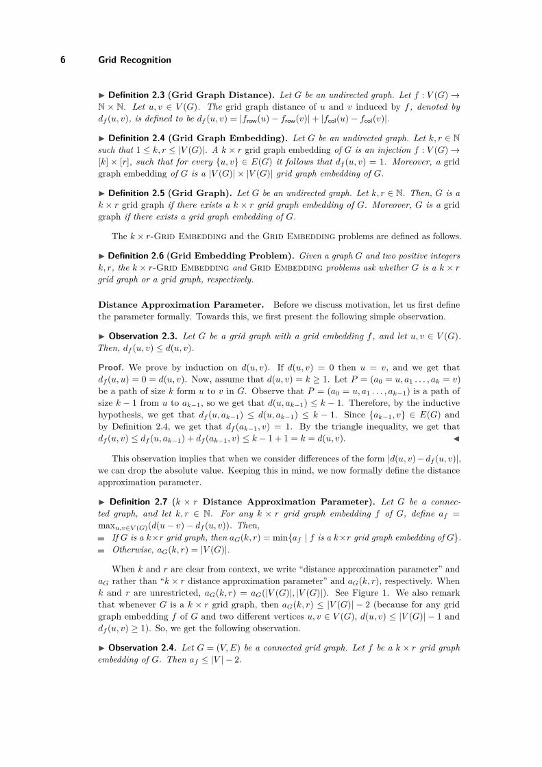
Distance Approximation Parameter. Before we discuss motivation, let us first definethe parameter formally. Towards this, we first present the following simple observation.
I Observation 2.3. Let G be a grid graph with a grid embedding f , and let u, v ∈ V (G).Then, df (u, v) ≤ d(u, v).
Proof. We prove by induction on d(u, v). If d(u, v) = 0 then u = v, and we get thatdf (u, u) = 0 = d(u, v). Now, assume that d(u, v) = k ≥ 1. Let P = (a0 = u, a1 . . . , ak = v)be a path of size k form u to v in G. Observe that P = (a0 = u, a1 . . . , ak−1) is a path ofsize k − 1 from u to ak−1, so we get that d(u, ak−1) ≤ k − 1. Therefore, by the inductivehypothesis, we get that df (u, ak−1) ≤ d(u, ak−1) ≤ k − 1. Since {ak−1, v} ∈ E(G) andby Definition 2.4, we get that df (ak−1, v) = 1. By the triangle inequality, we get thatdf (u, v) ≤ df (u, ak−1) + df (ak−1, v) ≤ k − 1 + 1 = k = d(u, v). J
This observation implies that when we consider differences of the form |d(u, v)− df (u, v)|,we can drop the absolute value. Keeping this in mind, we now formally define the distanceapproximation parameter.
I Definition 2.7 (k × r Distance Approximation Parameter). Let G be a connec-ted graph, and let k, r ∈ N. For any k × r grid graph embedding f of G, define af =maxu,v∈V (G)(d(u− v)− df (u, v)). Then,
If G is a k×r grid graph, then aG(k, r) = min{af | f is a k×r grid graph embedding of G}.Otherwise, aG(k, r) = |V (G)|.
When k and r are clear from context, we write “distance approximation parameter” andaG rather than “k × r distance approximation parameter” and aG(k, r), respectively. Whenk and r are unrestricted, aG(k, r) = aG(|V (G)|, |V (G)|). See Figure 1. We also remarkthat whenever G is a k × r grid graph, then aG(k, r) ≤ |V (G)| − 2 (because for any gridgraph embedding f of G and two different vertices u, v ∈ V (G), d(u, v) ≤ |V (G)| − 1 anddf (u, v) ≥ 1). So, we get the following observation.
I Observation 2.4. Let G = (V,E) be a connected grid graph. Let f be a k × r grid graphembedding of G. Then af ≤ |V | − 2.
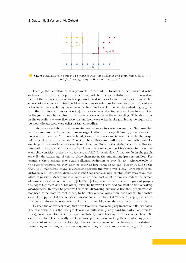
S.Gupta, G. Sa’ar and M. Zehavi 7
af1 = 6
af2 = 0
af3 = 0
Figure 1 Example of a path P on 8 vertices with three different grid graph embeddings f1, f2
and f3. Since af2 = af3 = 0, we get that aP = 0.
Clearly, the definition of this parameter is extendible to other embeddings and otherdistance measures (e.g., a plane embedding and the Euclidean distance). The motivationbehind the consideration of such a parameterization is as follows. First, we remark thatedges between vertices often model interactions or relations between entities. So, verticesadjacent in the graph may be required to be close to each other in the embedding (e.g., sothat they can interact more efficiently). On a more general note, vertices closer to each otherin the graph may be required to be closer to each other in the embedding. This also worksin the opposite way—vertices more distant from each other in the graph may be required tobe more distant from each other in the embedding.
This rationale behind this parameter makes sense in various scenarios. Suppose thatvertices represent utilities, factories or organizations, or, very differently, components tobe placed on a chip. On the one hand, those that are closer to each other in the graphmight need to cooperate more often: they have direct and indirect (through other entitieson the path) connections between them; the more “links on the chain”, the less is directedinteraction required. On the other hand, we may have a competitive constraint—we maywant these entities to also be “as far as possible”. In particular, if they are far in the graph,we will take advantage of this to place them far in the embedding (proportionally). Forexample, these entities may cause pollution, radiation or heat [8, 30]. Alternatively, inthe case of utilities, we may want to cover as large area as we can. Recently, due to theCOVID-19 pandemic, many governments around the world world have introduced socialdistancing. Briefly, social distancing means that people should be physically away from eachother, if possible. According to experts, one of the most effective ways to reduce the spreadof coronavirus is social distancing [13, 37, 50]. Suppose that the vertices represent people,the edges represent social (or other) relations between them, and we want to find a seatingarrangement. In order to preserve the social distancing, we would like that people who donot need to be close to each other, to be relatively far away from each other. In anotherexample, suppose that the vertices represent some facilities that “attract” people, like stores.Placing the stores far away from each other, if possible, contributes to social distancing.
Besides the above scenarios, there are two more motivating arguments of different flavor.The first argument is that the problem is computationally very hard (in particular, even fortrees), so we want to restrict it to get tractability, and this may be a reasonable choice. Soeven if we do not specifically want distance preservation, seeking those that comply withit is useful since it gives tractability. The second argument is that having such a distancepreserving embedding rather than any embedding can yield more efficient algorithms due
8 Grid Recognition
to special properties that it has. One such property is that computing distances betweenvertices in such an embedding can be done up to a small error (aG) in constant time.
We remark that the embeddings that our algorithms compute satisfy the conditions ofDefinition 2.4, in particular, the embeddings are planar. Furthermore, we do not need toknow the value of aG in advance, in order to use our algorithm, as we iterate over all thepotential values for aG.
Integer Linear Programming. In the Integer Linear Programming Feasibility(ILP) problem, the input consists of t variables x1, x2, . . . , xt and a set of m inequalities ofthe following form:
a1,1x1 +a1,2x1 +· · ·+a1,pxt≤ b1a2,1x1 +a2,2x2 +· · ·+a2,pxt≤ b2
......
......
am,1x1+am,2x2+· · ·+am,pxt≤bm
where all coefficients aij and bi are required to integers. The task is to check whether thereexists integer values for every variable xi so that all inequalities are satisfiable. The followingtheorem about the running time required to solve ILP will be useful in Section 3.
I Theorem 2.8 ([45, 44, 28]). An ILP instance of size n with p variables can be solved intime pO(p) · nO(1).
3 FPT Algorithm on General Graphs
In this section, we show that the k × r-Grid Embedding problem is FPT parameterizedby mcc(G) + k. We first give the definition of a k × r rectangular grid graph, which will beuseful throughout the section.
I Definition 3.1 (k × r Rectangular Grid Graph). An undirected graph H is a k × rrectangular grid graph if there exists a bijection f : V → [k]× [r], such that for every pair ofvertices u, v ∈ V (H), {v, u} ∈ E(H) if and only if df (u, v) = 1.
Given a k×r rectangular grid graph H and a corresponding bijective function f , we definethe columns of H as follows. For every i ∈ [k], j ∈ [r], Cj(H) = {u ∈ V (H)|fcol(u) = j}.It is easy to see that the vertex set of H can be denoted as the union of columns, i.e.V (H) =
⋃rj=1 Cj(H). We refer to C1(H) and Cr(H) as the left boundary column and right
boundary column, respectively, of H.Given a subgraph S of a k × r rectangular grid graph H, we denote the set of fully
contained connected components of S, i.e. all the connected components of S that either donot intersect the boundary columns of H or intersect both boundary columns of H, by FC(S).Similarly, we denote the set of left contained (right contained) connected components of S, i.e.all the connected components of S that intersect the left (right) boundary column of H butdo not intersect the right (left) boundary column of H, by LC(S) (RC(S)). Note that thethree sets FC(S),LC(S) and RC(S) are pairwise disjoint and S = FC(S) ∪ LC(S) ∪RC(S).See Figure 2.
I Theorem 1.1. k × r-Grid Embedding is FPT parameterized by mcc + k where mcc isthe maximum size of a connected component in the input graph.
Proof. The FPT algorithm is based on ILP. To this end, let G be an instance of the k×r-GridEmbedding problem. We first give an overview of the ideas behind the algorithm.
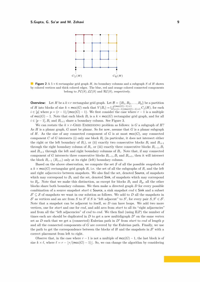
S.Gupta, G. Sa’ar and M. Zehavi 9
C1(H) C6(H)
Figure 2 A 5× 6 rectangular grid graph H, its boundary columns and a subgraph S of H shownby colored vertices and thick colored edges. The blue, red and orange colored connected components
belong to FC(S),LC(S) and RC(S), respectively.
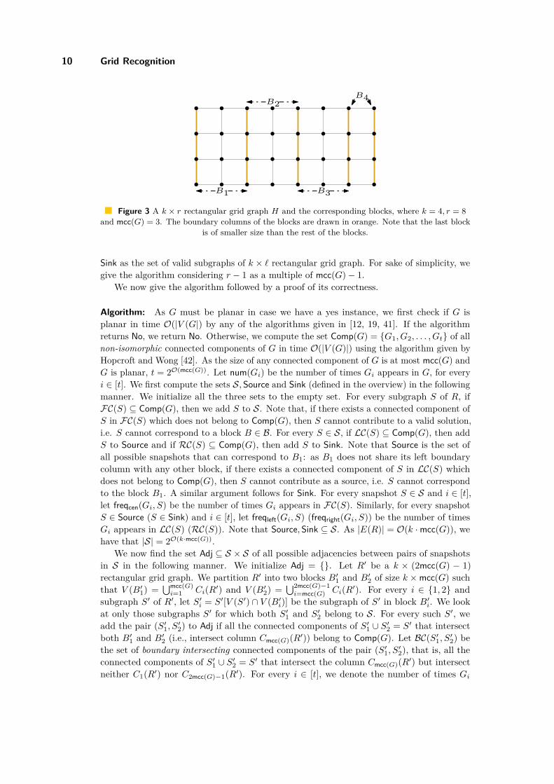
Overview: Let H be a k×r rectangular grid graph. Let B = {B1, B2, . . . , Bp} be a partitionof H into blocks of size k ×mcc(G) such that V (Bi) =
⋃i(mcc(G)−1)+1j=(i−1)(mcc(G)−1)+1 Cj(H), for each
i ∈ [p] where p = (r − 1)/(mcc(G)− 1). We first consider the case where r − 1 is a multipleof mcc(G)− 1. Note that each block Bi is a k ×mcc(G) rectangular grid graph, and for alli ∈ [p− 1], Bi and Bi+1 share a boundary column. See Figure 3.
We can restate the k × r-Grid Embedding problem as follows: is G a subgraph of H?As H is a planar graph, G must be planar. So for now, assume that G is a planar subgraphof H. As the size of any connected component of G is at most mcc(G), any connectedcomponent C of G intersects (i) only one block Bi (in particular, it does not intersect eitherthe right or the left boundary of Bi), or (ii) exactly two consecutive blocks Bi and Bi+1through the right boundary column of Bi, or (iii) exactly three consecutive blocks Bi−1, Biand Bi+1 through the left and right boundary columns of Bi. Note that, if any connectedcomponent of G intersects three consecutive blocks Bi−1, Bi and Bi+1, then it will intersectthe block Bi−1 (Bi+1) only at its right (left) boundary column.
Based on the above observation, we compute the set S of all the possible snapshots ofa k ×mcc(G) rectangular grid graph R, i.e. the set of all the subgraphs of R, and the leftand right adjacencies between snapshots. We also find the set, denoted Source, of snapshotswhich may correspond to B1 and the set, denoted Sink, of snapshots which may correspondto Bp. Note that we make this distinction, as except for blocks B1 and Bp, all the otherblocks share both boundary columns. We then make a directed graph D for every possiblecombination of a source snapshot start ∈ Source, a sink snapshot end ∈ Sink and a subsetS ′ ⊆ S of snapshots we want in our solution as follows. We add to D all the snapshots inS ′ as vertices and an arc from S to S′ if S is “left adjacent” to S′, for every pair S, S′ ∈ S ′.Note that a snapshot can be adjacent to itself, so D can have loops. We add two morevertices, one for start and one for end, and add arcs from start to all its “right adjacencies”and from all the “left adjacencies” of end to end. We then find (using ILP) the number oftimes each arc should be duplicated in D to get a new multidigraph D′ on the same vertexset as D such that we get a (connected) Eulerian path in D′ from start to end of length pand all the connected components of G are covered by the Eulerian path. Finally, we usethe path to get the correspondence between the blocks of H and the snapshots in S ′ with acorrect placement from left to right.
Observe that, in the case where r − 1 is not a multiple of mcc(G)− 1, the last block is ofsize k × `, where ` = r − br/(mcc(G)− 1)c. So, we can change the algorithm by considering
10 Grid Recognition
B1
B2
B3
B4
Figure 3 A k × r rectangular grid graph H and the corresponding blocks, where k = 4, r = 8and mcc(G) = 3. The boundary columns of the blocks are drawn in orange. Note that the last block
is of smaller size than the rest of the blocks.
Sink as the set of valid subgraphs of k × ` rectangular grid graph. For sake of simplicity, wegive the algorithm considering r − 1 as a multiple of mcc(G)− 1.
We now give the algorithm followed by a proof of its correctness.
Algorithm: As G must be planar in case we have a yes instance, we first check if G isplanar in time O(|V (G|) by any of the algorithms given in [12, 19, 41]. If the algorithmreturns No, we return No. Otherwise, we compute the set Comp(G) = {G1, G2, . . . , Gt} of allnon-isomorphic connected components of G in time O(|V (G)|) using the algorithm given byHopcroft and Wong [42]. As the size of any connected component of G is at most mcc(G) andG is planar, t = 2O(mcc(G)). Let num(Gi) be the number of times Gi appears in G, for everyi ∈ [t]. We first compute the sets S,Source and Sink (defined in the overview) in the followingmanner. We initialize all the three sets to the empty set. For every subgraph S of R, ifFC(S) ⊆ Comp(G), then we add S to S. Note that, if there exists a connected component ofS in FC(S) which does not belong to Comp(G), then S cannot contribute to a valid solution,i.e. S cannot correspond to a block B ∈ B. For every S ∈ S, if LC(S) ⊆ Comp(G), then addS to Source and if RC(S) ⊆ Comp(G), then add S to Sink. Note that Source is the set ofall possible snapshots that can correspond to B1: as B1 does not share its left boundarycolumn with any other block, if there exists a connected component of S in LC(S) whichdoes not belong to Comp(G), then S cannot contribute as a source, i.e. S cannot correspondto the block B1. A similar argument follows for Sink. For every snapshot S ∈ S and i ∈ [t],let freqcen(Gi, S) be the number of times Gi appears in FC(S). Similarly, for every snapshotS ∈ Source (S ∈ Sink) and i ∈ [t], let freqleft(Gi, S) (freqright(Gi, S)) be the number of timesGi appears in LC(S) (RC(S)). Note that Source,Sink ⊆ S. As |E(R)| = O(k ·mcc(G)), wehave that |S| = 2O(k·mcc(G)).
We now find the set Adj ⊆ S × S of all possible adjacencies between pairs of snapshotsin S in the following manner. We initialize Adj = {}. Let R′ be a k × (2mcc(G) − 1)rectangular grid graph. We partition R′ into two blocks B′1 and B′2 of size k ×mcc(G) suchthat V (B′1) =
⋃mcc(G)i=1 Ci(R′) and V (B′2) =
⋃2mcc(G)−1i=mcc(G) Ci(R′). For every i ∈ {1, 2} and
subgraph S′ of R′, let S′i = S′[V (S′) ∩ V (B′i)] be the subgraph of S′ in block B′i. We lookat only those subgraphs S′ for which both S′1 and S′2 belong to S. For every such S′, weadd the pair (S′1, S′2) to Adj if all the connected components of S′1 ∪ S′2 = S′ that intersectboth B′1 and B′2 (i.e., intersect column Cmcc(G)(R′)) belong to Comp(G). Let BC(S′1, S′2) bethe set of boundary intersecting connected components of the pair (S′1, S′2), that is, all theconnected components of S′1 ∪ S′2 = S′ that intersect the column Cmcc(G)(R′) but intersectneither C1(R′) nor C2mcc(G)−1(R′). For every i ∈ [t], we denote the number of times Gi
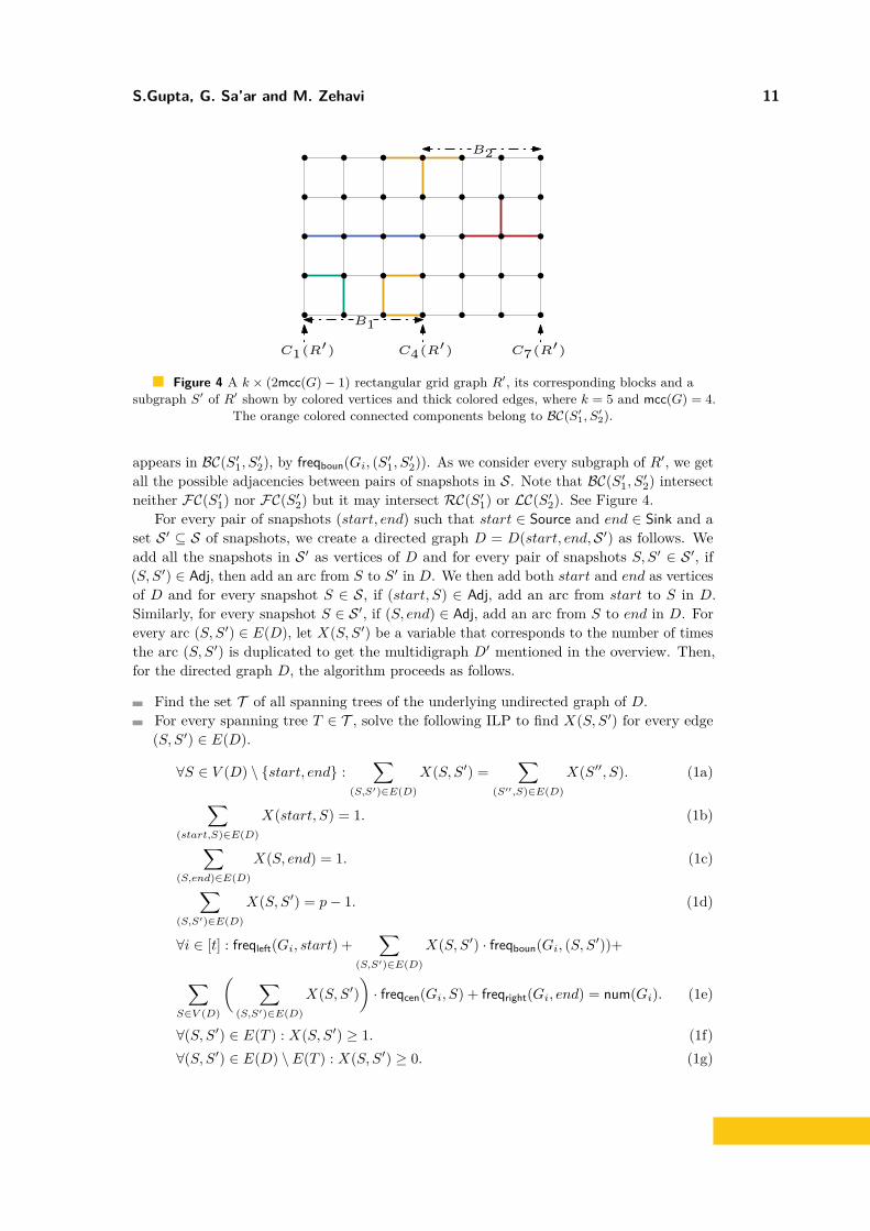
S.Gupta, G. Sa’ar and M. Zehavi 11
B1
B2
C1(R′) C4(R′) C7(R′)
Figure 4 A k × (2mcc(G)− 1) rectangular grid graph R′, its corresponding blocks and asubgraph S′ of R′ shown by colored vertices and thick colored edges, where k = 5 and mcc(G) = 4.
The orange colored connected components belong to BC(S′1, S
′2).
appears in BC(S′1, S′2), by freqboun(Gi, (S′1, S′2)). As we consider every subgraph of R′, we getall the possible adjacencies between pairs of snapshots in S. Note that BC(S′1, S′2) intersectneither FC(S′1) nor FC(S′2) but it may intersect RC(S′1) or LC(S′2). See Figure 4.
For every pair of snapshots (start, end) such that start ∈ Source and end ∈ Sink and aset S ′ ⊆ S of snapshots, we create a directed graph D = D(start, end,S ′) as follows. Weadd all the snapshots in S ′ as vertices of D and for every pair of snapshots S, S′ ∈ S ′, if(S, S′) ∈ Adj, then add an arc from S to S′ in D. We then add both start and end as verticesof D and for every snapshot S ∈ S, if (start, S) ∈ Adj, add an arc from start to S in D.Similarly, for every snapshot S ∈ S ′, if (S, end) ∈ Adj, add an arc from S to end in D. Forevery arc (S, S′) ∈ E(D), let X(S, S′) be a variable that corresponds to the number of timesthe arc (S, S′) is duplicated to get the multidigraph D′ mentioned in the overview. Then,for the directed graph D, the algorithm proceeds as follows.
Find the set T of all spanning trees of the underlying undirected graph of D.For every spanning tree T ∈ T , solve the following ILP to find X(S, S′) for every edge(S, S′) ∈ E(D).
∀S ∈ V (D) \ {start, end} :∑
(S,S′)∈E(D)
X(S, S′) =∑
(S′′,S)∈E(D)
X(S′′, S). (1a)
∑(start,S)∈E(D)
X(start, S) = 1. (1b)
∑(S,end)∈E(D)
X(S, end) = 1. (1c)
∑(S,S′)∈E(D)
X(S, S′) = p− 1. (1d)
∀i ∈ [t] : freqleft(Gi, start) +∑
(S,S′)∈E(D)
X(S, S′) · freqboun(Gi, (S, S′))+
∑S∈V (D)
( ∑(S,S′)∈E(D)
X(S, S′))· freqcen(Gi, S) + freqright(Gi, end) = num(Gi). (1e)
∀(S, S′) ∈ E(T ) : X(S, S′) ≥ 1. (1f)∀(S, S′) ∈ E(D) \ E(T ) : X(S, S′) ≥ 0. (1g)
12 Grid Recognition
If the ILP returns a feasible solution, then return Yes.Recall that we run the algorithm for every possible D. If none of them returns Yes, we returnNo.
Correctness: We start by analyzing the equations. Equation 1f ensures that the digraphD′ is connected, and, in this context, recall that we go over all the possible spanning trees tocheck all the different possible connectivities between the vertices of D′. Equations 1a, 1band 1c ensure that there exists an Eulerian path in D from start to end. Equation 1d ensuresthat the total number of edges in D′ is p− 1, which in turn means that the Eulerian pathfrom start to end in D′ is of length p, which is equal to the number of required blocks. Givena multidigraph D′, each connected component of G can contribute to only one set out ofLC(start),RC(end),FC(S) and B(S′, S′′), for S, S′, S′′ ∈ S ′ such that (S′, S′′) ∈ E(D), asthere exists no S ∈ S ′ such that (S, start) ∈ E(D) or (end, S) ∈ E(D). So, Equation 1eensures that all the connected components of G are covered by the path exactly once.
Next, we prove that the algorithm is correct. In one direction, assume that the algorithmreturns Yes. This means that for some directed graph D, ILP assigned integer values forthe variables X(S, S′), (S, S′) ∈ E(D) such that the corresponding multidigraph D′ has anEulerian path from start to end of size p covering all the connected components of G exactlyonce. Let P = (S1 = start, S2, . . . , Sp−1, Sp = end) be the Eulerian path from start to endin D′, where Si ∈ S ′ for every i ∈ [p]. Then, we can define V (G) ∩ V (Bi) = V (Si), for everyi ∈ [p]. Observe that, G =
⋃i∈[p](G ∩Bi). Thus G is a subgraph of H, i.e. G is a k × r grid
graph.Conversely, let G be a k × r grid graph, i.e. G is a subgraph of H. For every i ∈ [p], let
SH = {H1, H2, . . . ,Hp} be the set of graphs Hi = G[V (G) ∩ V (Bi)]. For every i ∈ [p] andj ∈ [p − 1], observe that Hi ∈ S and (Hj , Hj+1) ∈ Adj. Now, let P = (v1, v2, . . . , vp) be adirected path where vi is a vertex corresponding to the graph Hi. We create a multidigraphfrom P by repeating the following procedure. If there exist two vertices v, v′ ∈ V (P )\{v1, vp}such that the corresponding graphs in SH are isomorphic, then do a join(v, v′) on P . LetD′H be the multidigraph obtained after the above procedure. Note that D′H has an Eulerianpath from v1 to vp of length vp. Let DH be the multigraph obtained by D′H be removingmultiple arcs between any pair of vertices by a single directed edge. For every e ∈ E(D), letXH(e) be the number of times the arc e appears in D′H . Thus, the algorithm return willreturn Yes for DH and the corresponding XH(e) values for every e ∈ E(D).
For a given directed graph D, |T | = |V (D)||V (D)−2| and number of variables X(e), forevery e ∈ E(D), is O(|V (D)|2). As S = 2O(k·mcc(G)), number of different directed graphs Dis 22O(k·mcc(G)) and |V (D)| = 2O(k·mcc(G)) for any directed graph D. So, by Theorem 2.8, thek × r-Grid Embedding problem is FPT parameterized by mcc(G) + k. J
The following claim about 2-Strip Packing will follow from the Theorem 1.1, as weprove below.
I Corollary 1.2. 2-Strip Packing is FPT parameterized by `+ k where ` is the maximumof the dimensions of the input rectangles.
Proof. Without loss of generality, we can assume that there does not exist any input rectangleof size 1× t, where t ≤ `, as otherwise we can get an equivalent instance of 2-Strip Packingby multiplying each of the dimensions of the input rectangles and of the strip by 2. For eachinput rectangle, we create a length× breath rectangular grid graph, where length and breathare the dimensions of the input rectangle such that length ≤ breath. Let G be the disjointunion of the graphs corresponding to the input rectangles. Observe that mcc(G) = `2, as

S.Gupta, G. Sa’ar and M. Zehavi 13
+
–0 vol
1 vol
Figure 5 A (1, 0) battery.
the size of any graph corresponding to a input rectangle is at most `2. So, by Theorem 1.1,2-Strip Packing is FPT parameterized by `+ k. J
Note that when k and r are unrestricted, we can embed each connected componentindividually in FPT time (e.g., by using brute-force), so we directly get the followingobservation from the Theorem 1.1.
I Observation 1.1. Grid Embedding is FPT parameterized by mcc where mcc is themaximum size of a connected component in the input graph.
Given a graph G, if G is a (k × r) grid graph then ∆(G) ≤ 4. So, by the Observation 2.2and the Theorem 1.1, we get the following corollary.
I Corollary 1.3. k × r-Grid Embedding is FPT parameterized by td + k, and GridEmbedding is FPT parameterized by td, where td is the treedepth of the input graph.
4 Distance Approximation Parameter
In this section, we consider the distance approximation parameter and prove Theorems 1.4,1.5 and 1.6. We remark that the embeddings that our algorithms compute satisfy theconditions of Definition 2.4, in particular, the embeddings are planar (being grid graphs).
4.1 Para-NP-hardness with Respect to aG on General GraphsWe show a reduction from SAT to Grid Embedding where if the output is a yes-instance,then the parameter aG of the output graph is upper bounded by a constant. In order tomake the reduction clearer, instead of presenting a direct reduction from SAT to GridEmbedding, we present a two-stage reduction. To this end, we define a simple problemcalled the Batteries problem. We first give a reduction from SAT to the Batteriesproblem, and then we give a reduction from the Batteries problem to Grid Embedding.
We start with the description of the Batteries problem. A battery has two sides, apositive side and a negative side, denoted by + and -, respectively. Each side of a batteryhas voltage of one or zero volts. Formally, a battery is represented by a boolean pair, definedas follows. See Figure 5 for an illustration.
I Definition 4.1 (Battery). A battery B is a boolean pair B = (x1, x2), x1, x2 ∈ {0, 1},where x1 is the voltage of the positive side of B (called the positive voltage) and x2 is thevoltage of the negative side of B (called the negative voltage).
14 Grid Recognition
Figure 6 A (4, 3) battery holder.
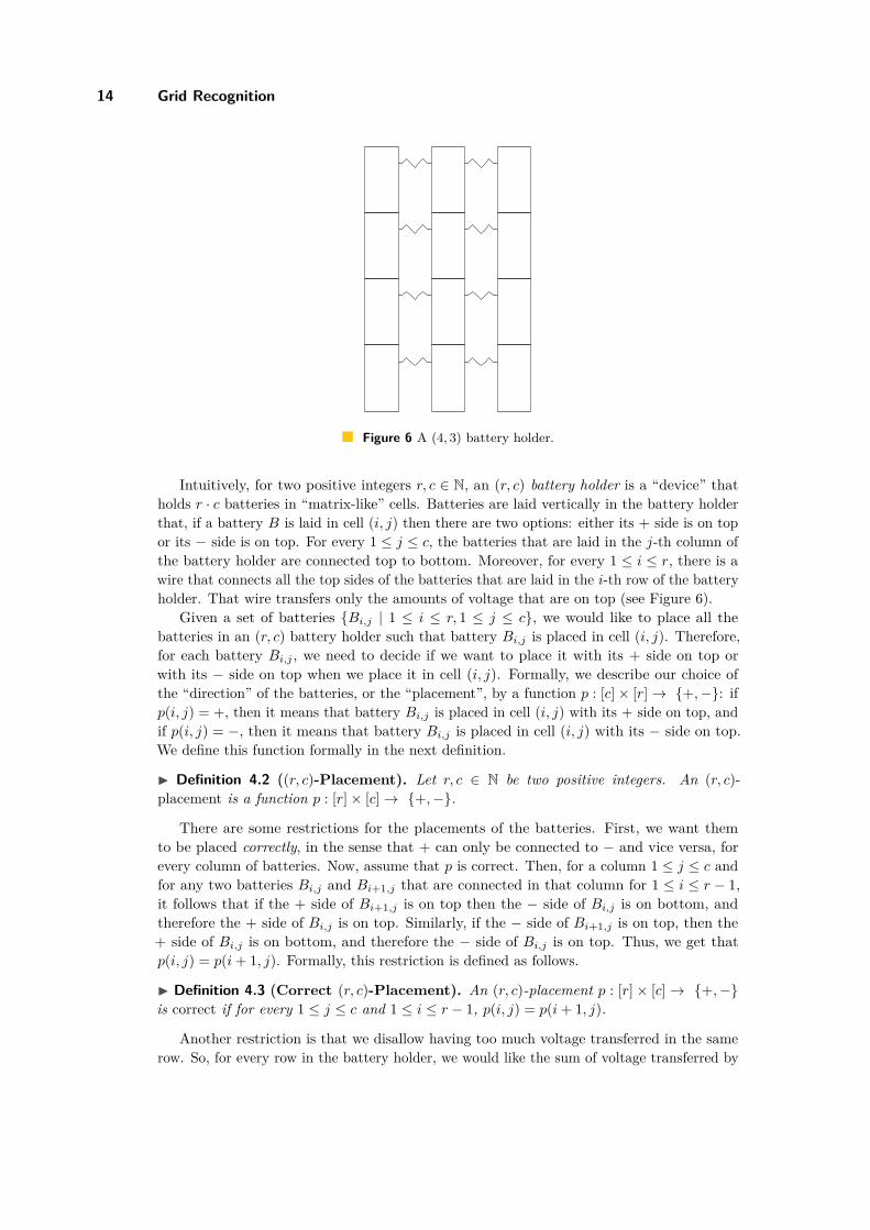
Intuitively, for two positive integers r, c ∈ N, an (r, c) battery holder is a “device” thatholds r · c batteries in “matrix-like” cells. Batteries are laid vertically in the battery holderthat, if a battery B is laid in cell (i, j) then there are two options: either its + side is on topor its − side is on top. For every 1 ≤ j ≤ c, the batteries that are laid in the j-th column ofthe battery holder are connected top to bottom. Moreover, for every 1 ≤ i ≤ r, there is awire that connects all the top sides of the batteries that are laid in the i-th row of the batteryholder. That wire transfers only the amounts of voltage that are on top (see Figure 6).
Given a set of batteries {Bi,j | 1 ≤ i ≤ r, 1 ≤ j ≤ c}, we would like to place all thebatteries in an (r, c) battery holder such that battery Bi,j is placed in cell (i, j). Therefore,for each battery Bi,j , we need to decide if we want to place it with its + side on top orwith its − side on top when we place it in cell (i, j). Formally, we describe our choice ofthe “direction” of the batteries, or the “placement”, by a function p : [c]× [r]→ {+,−}: ifp(i, j) = +, then it means that battery Bi,j is placed in cell (i, j) with its + side on top, andif p(i, j) = −, then it means that battery Bi,j is placed in cell (i, j) with its − side on top.We define this function formally in the next definition.
I Definition 4.2 ((r, c)-Placement). Let r, c ∈ N be two positive integers. An (r, c)-placement is a function p : [r]× [c]→ {+,−}.
There are some restrictions for the placements of the batteries. First, we want themto be placed correctly, in the sense that + can only be connected to − and vice versa, forevery column of batteries. Now, assume that p is correct. Then, for a column 1 ≤ j ≤ c andfor any two batteries Bi,j and Bi+1,j that are connected in that column for 1 ≤ i ≤ r − 1,it follows that if the + side of Bi+1,j is on top then the − side of Bi,j is on bottom, andtherefore the + side of Bi,j is on top. Similarly, if the − side of Bi+1,j is on top, then the+ side of Bi,j is on bottom, and therefore the − side of Bi,j is on top. Thus, we get thatp(i, j) = p(i+ 1, j). Formally, this restriction is defined as follows.
I Definition 4.3 (Correct (r, c)-Placement). An (r, c)-placement p : [r]× [c]→ {+,−}is correct if for every 1 ≤ j ≤ c and 1 ≤ i ≤ r − 1, p(i, j) = p(i+ 1, j).
Another restriction is that we disallow having too much voltage transferred in the samerow. So, for every row in the battery holder, we would like the sum of voltage transferred by
S.Gupta, G. Sa’ar and M. Zehavi 15
the wire of that row to be at most c− 1. For a set of batteries {Bi,j | 1 ≤ i ≤ r, 1 ≤ j ≤ c}and an (r, c)-placement p, we denote the voltage transferred from battery Bi,j placed in cell(i, j) by Vp(i, j). Therefore, it follows that if Bi,j = (x(i,j)
1 , x(i,j)2 ), then if p(i, j) = + then
Vp(i, j) = x(i,j)1 , and if p(i, j) = − then Vp(i, j) = x
(i,j)2 . We define this restriction as follows.
I Definition 4.4 (Safe (r, c)-Placement). Let B = {Bi,j = (x(i,j)1 , x
(i,j)2 ) | 1 ≤ i ≤ r, 1 ≤
j ≤ c} be a set of batteries. An (r, c)-placement. p : [r]× [c]→ {+,−} is safe with respectto B if for every 1 ≤ i ≤ r it follows that
∑cj=1 Vp(i, j) ≤ c− 1.
When B is clear from the context, we refer to a safe placement with respect to B simplyas a safe placement.
We define the Batteries problem in the next definition.
I Definition 4.5 (The Batteries Problem). Given a set of batteries B = {Bi,j =(x(i,j)
1 , x(i,j)2 ) | 1 ≤ i ≤ r, 1 ≤ j ≤ c}, does there exist an (r, c)-placement p that is cor-
rect and safe?
Reduction from SAT to Batteries. We now give a polynomial reduction, called reduce1,from SAT to the Batteries problem.
Given an instance π of SAT with n variables x1, . . . , xn and m clauses µ1, . . . , µm,reduce1(π) = Bπ where Bπ is a set of batteries Bπ = {Bi,j = (x(i,j)
1 , x(i,j)2 ) | 1 ≤ i ≤ m, 1 ≤
j ≤ n} defined as follows. For every 1 ≤ i ≤ m, 1 ≤ j ≤ n, we set x(i,j)1 = 0 if the literal xj
appears in µi, and we set x(i,j)1 = 1 otherwise. Similarly, for every 1 ≤ i ≤ m, 1 ≤ j ≤ n, we
set x(i,j)2 = 0 if the literal x̄j appears in µi, and we set x(i,j)
2 = 1 otherwise.It is clear that this reduction is polynomial, as we state in the next observation.
I Observation 4.1. Let π be an instance of SAT. Then the function reduce1 on π can becomputed in time polynomial in |π|.
Towards the proof of the correctness of this reduction, we have the next simple lemma.We show that if an (r, c)-placement p is correct, then all the batteries in every column areplaced in the same direction. Note that the converse side, that is, that if all the batteries inevery column are placed in the same direction, then p is correct, is trivial.
I Lemma 4.6. An (r, c)-placement p is correct if and only if for every 1 ≤ j ≤ c there existspj ∈ {+,−} such that for every 1 ≤ i ≤ r it follows that p(i, j) = pj.
Proof. Let p be a correct (r, c)-placement. Let 1 ≤ j ≤ c. We set pj = p(1, j). We showby induction that for every 1 ≤ i ≤ r it follows that p(i, j) = pj . The basic case is trivialsince pj = p(1, j). Let 1 < i ≤ r. By the inductive hypothesis, it follows that p(i− 1, j) = pj .Since p is correct it follows that p(i− 1, j) = p(i, j). Therefore, we get that p(i, j) = pj . Theother direction of the lemma is trivial. J
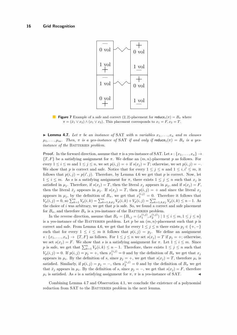
From Lemma 4.6 we get that if p is correct, then for every column of the battery holder,we have that all the batteries are placed with either their + on top or their − on top. Forevery 1 ≤ j ≤ c, we refer to pj from Lemma 4.6 as the placement of column j. The placementof every column 1 ≤ j ≤ n corresponds to a placement for xj , that is, pj = + corresponds toxj = T and pj = − corresponds to xj = F . Every row 1 ≤ i ≤ m of batteries in the batteryholder corresponds to clause µi from π. In order to get a safe placement, we need at leastone battery with zero voltage on its top side. This corresponds to having at least one literalthat is satisfied in each clause of π. See Figure 7.
In the next lemma we prove the correctness of the reduction.
16 Grid Recognition
+
–+
–
+
–
+
–
0 vol
1 vol
0 vol
1 vol
0 vol
1 vol0 vol
1 vol
Figure 7 Example of a safe and correct (2, 2)-placement for reduce1(π) = Bπ whereπ = (x̄1 ∨ x2) ∧ (x1 ∨ x2). This placement corresponds to x1 = F, x2 = T .
I Lemma 4.7. Let π be an instance of SAT with n variables x1, . . . , xn and m clausesµ1, . . . , µm. Then, π is a yes-instance of SAT if and only if reduce1(π) = Bπ is a yes-instance of the Batteries problem.
Proof. In the forward direction, assume that π is a yes-instance of SAT. Let s : {x1, . . . , xn} →{T, F} be a satisfying assignment for π. We define an (m,n)-placement p as follows. Forevery 1 ≤ i ≤ m and 1 ≤ j ≤ n, we set p(i, j) = + if s(xj) = T ; otherwise, we set p(i, j) = −.We show that p is correct and safe. Notice that for every 1 ≤ j ≤ n and 1 ≤ i, i′ ≤ m, itfollows that p(i, j) = p(i′, j). Therefore, by Lemma 4.6 we get that p is correct. Now, let1 ≤ i ≤ m. As s is a satisfying assignment for π, there exists 1 ≤ j ≤ n such that xj issatisfied in µj . Therefore, if s(xj) = T , then the literal xj appears in µj , and if s(xj) = F ,then the literal x̄j appears in µj . If s(xj) = T , then p(i, j) = + and since the literal xjappears in µj , by the definition of Bπ, we get that x(i,j)
1 = 0. Therefore it follows thatVp(i, j) = 0, so
∑nk=1 Vp(i, k) =
∑nk=1,k 6=j Vp(i, k) +Vp(i, j) =
∑nk=1,k 6=j Vp(i, k) ≤ n− 1. As
the choice of i was arbitrary, we get that p is safe. So, we found a correct and safe placementfor Bπ, and therefore Bπ is a yes-instance of the Batteries problem.
In the reverse direction, assume that Bπ = {Bi,j = (x(i,j)1 , x
(i,j)2 ) | 1 ≤ i ≤ m, 1 ≤ j ≤ n}
is a yes-instance of the Batteries problem. Let p be an (m,n)-placement such that p iscorrect and safe. From Lemma 4.6, we get that for every 1 ≤ j ≤ n there exists pj ∈ {+,−}such that for every 1 ≤ i ≤ m it follows that p(i, j) = pj . We define an assignments : {x1, . . . , xn} → {T, F} as follows. For 1 ≤ j ≤ n we set s(xj) = T if pj = +; otherwise,we set s(xj) = F . We show that s is a satisfying assignment for π. Let 1 ≤ i ≤ m. Sincep is safe, we get that
∑nk=1 Vp(i, k) ≤ n − 1. Therefore, there exists 1 ≤ j ≤ n such that
Vp(i, j) = 0. If p(i, j) = pj = +, then x(i,j)1 = 0 and by the definition of Bπ we get that xj
appears in µi. By the definition of s, since pj = +, we get that s(xj) = T , therefore µi issatisfied. Similarly, if p(i, j) = pj = −, then x(i,j)
2 = 0 and by the definition of Bπ we getthat x̄j appears in µi. By the definition of s, since pj = −, we get that s(xj) = F , thereforeµi is satisfied. As s is a satisfying assignment for π, π is a yes-instance of SAT. J
Combining Lemma 4.7 and Observation 4.1, we conclude the existence of a polynomialreduction from SAT to the Batteries problem in the next lemma.
S.Gupta, G. Sa’ar and M. Zehavi 17
I Corollary 4.8. There exists a polynomial reduction from SAT to the Batteries problem.
Reduction from Batteries to Grid Embedding. We now give a polynomial reductionfrom the Batteries problem to Grid Embedding where the output graph satisfies thataG is bounded by a fixed constant (if it is a yes-instance). 2
For this purpose, we present the battery gadget (see Figures 8 and 9). The battery gadgetis composed of a 13× 9 rectangle, which corresponds to a cell in the battery holder. It has apositive side and a negative side, which correspond to battery sides, and two wire verticesthat correspond to the wire that transfers voltage in the battery holder. In addition, thereare six synchronization edges attached to the top and bottom sides of the rectangle. Aswe will see, the synchronization edges make every two vertically adjacent battery gadget“synchronized”, similarly to the + and − sides of a battery. On the top and bottom sidesof the gadget we have the option to add an extra edge, called the positive voltage andthe negative voltage, respectively; see Figure 8. These edges correspond to the voltage ofeach side of the battery, that is, we add the positive (negative) voltage if and only if thevoltage of the positive (negative) side of the battery is one. We denote the battery gadget byH = (x1, x2), x1, x2 ∈ {0, 1}, where x1 = 1 if and only if we added the positive voltage, andx2 = 1 if and only if we added the negative voltage. Observe that H = (x1, x2) correspondsto the battery B = (x1, x2), as exemplified in Figure 9.
Next, we define a graph called m× n-grid frame (see Figure 10).
I Definition 4.9 (An m×n-Grid Frame). Let m,n ∈ N. An m×n-grid frame is the graphGm,n = (Vm,n, Em,n) where Vm,n = {(k, `) | 0 ≤ k ≤ 2, 0 ≤ ` ≤ 8·n+4}∪{(k, `) | 12·m+2 ≤k ≤ 12 ·m+ 4, 0 ≤ ` ≤ 8 · n+ 4} ∪ {(k, `) | 0 ≤ k ≤ 12 ·m+ 4, 0 ≤ ` ≤ 2} ∪ {(k, `) | 0 ≤ k ≤12 ·m+ 4, 8 · n+ 2 ≤ ` ≤ 8 · n+ 4} and Em,n = {{(r, c), (r′, c′)} | (r, c), (r′, c′) ∈ Vm,n and|r − r′|+ |c− c′| = 1}.
Let m,n ∈ N be two positive integers. Given a set of battery gadgets H = {Hi,j =(x(i,j)
1 , x(i,j)2 ) | 1 ≤ i ≤ m, 1 ≤ j ≤ n}, we denote by GH (when H is clear from the context
we refer to GH simply as G) the following graph. The graph G is composed of m · n batterygadgets that are ordered in a “matrix shape”, i.e. the battery gadget Hi,j is located at thei-th “row” and the j-th “column” (see Figures 13 and 12). For every 1 ≤ i < m the batterygadgets Hi,j and Hi+1,j share one side of their rectangles, that is, the bottom side of therectangle of Hi,j is the top side of the rectangle of Hi+1,j . Similarly, for every 1 ≤ j < n
the battery gadgets Hi,j and Hi,j+1 share one side of their rectangles, that is, the right sideof the rectangle of Hi,j is the left side of the rectangle of Hi,j+1. In addition, the “matrix”of battery gadgets is encircled by an m × n-grid frame (see Figures 13 and 12). Lastly,we delete some of the top and bottom synchronization edges we do not need, i.e. thosewhich are not attached to an side that is shared by two rectangles. More precisely, for every1 ≤ j ≤ n we delete the three edges attached to the top side of the rectangle of B1,j andthe three edges attached to the bottom side of the rectangle of Bm,j . Observe that eachsynchronization vertex is common to two battery gadgets. That is, for every 1 ≤ i < m and1 ≤ j ≤ n, the synchronization vertices 3, 4, 5 (see Figure 8)of the battery gadget Hi+1,jare the synchronization vertices 6, 7, 8 of Hi,j , respectively. Therefore, when we considerthe graph GH and not only an arbitrary battery gadget, we denote these synchronizationvertices by Si,j(1), Si,j(2), Si,j(3) for every 1 ≤ i < m and 1 ≤ j ≤ n. Similarly, when we
2 So, if aG is not bounded by that constant, we can output a trivial no-instance where it is bounded bythat constant and hence ensure that aG is always bounded by that constant.

18 Grid Recognition
1 2
3 4 5
6 7 8Figure 8 The battery gadget. The positive side is in blue and the negative side is in red. The
wire is green. The positive voltage is in dashed blue and the negative voltage is in dashed red.
consider the graph GH and not only an arbitrary battery gadget, we denote the wire vertices1 and 2 by W (i, j) for every 1 ≤ i ≤ m and 0 ≤ j ≤ n (see Figure 11).
Given an instance of the Batteries problem B = {Bi,j = (x(i,j)1 , x
(i,j)2 ) | 1 ≤ i ≤
m, 1 ≤ j ≤ n}, we denote by HB the corresponding set of battery gadgets of B, that isHB = {Hi,j = (x(i,j)
1 , x(i,j)2 ) | 1 ≤ i ≤ m, 1 ≤ j ≤ n}. We are ready to present our reduction
function reduce2: reduce2(B) = GHB. See Figures 13 and 12 for illustration. To simplify the
notation, we denote the graph GHBby GB .
It is easy to see that this reduction is polynomial, as we state in the next observation.
I Observation 4.2. Let B be an instance of the Batteries problem. Then, the functionreduce2 works in time polynomial in |B|.
Now we turn to prove the correctness of the reduction. First, we distinguish betweensome “parts” of the graph that have a fixed embedding to other parts that might have morethan one way to be embedded. First, we show that the embedding of the m×n-grid frame is“almost fixed”. Formally, in the following lemma we show that the embedding is fixed oncewe choose an embedding of three vertices. Intuitively, the “shape” of the m× n-grid frame isfixed in every embedding, but we may “rotate” the frame 90, 180 or 270 degrees, or “move”it to another “location”, but this does not matter for our purposes.
I Lemma 4.10. Let m,n ∈ N be two positive integers. Let f be a grid graph embeddingof an m × n-grid frame Gm,n = (Vm,n, Em,n). If f((0, 0)) = (0, 0) f((1, 0)) = (1, 0) andf((1, 1)) = (1, 1), then for every (r, c) ∈ Vm,n it follows that f((r, c)) = (r, c).

S.Gupta, G. Sa’ar and M. Zehavi 19
Figure 9 A (1, 0) battery gadget.
(0, 0) (0, 10) (0, 20)
(16, 20)(16, 0) (16, 10)
Figure 10 A (1× 2)-grid frame.
Proof. First we prove the lemma for the “top edge” of the m × n-grid frame, that is{(k, `) | 0 ≤ k ≤ 2, 0 ≤ ` ≤ 8 · n + 4} ⊆ Vm,n. We show by induction on j that for every1 ≤ j ≤ 8 · n + 4 it follows that: for every 0 ≤ ` ≤ j and 0 ≤ k ≤ 2, we have thatf((`, k)) = (`, k).
The base case is where j = 1. Observe that {(0, 1), (1, 1)}, {(0, 1), (0, 0)} ∈ Em,n,therefore df ((0, 1), (1, 1)) = |frow(0, 1)− frow(1, 1)|+ |fcol(0, 1)− fcol(1, 1)| = |frow(0, 1)− 1|+|frow(0, 1)−1| = 1, and also df ((0, 1), (0, 0)) = |frow(0, 1)−frow(0, 0)|+ |fcol(0, 1)−fcol(1, 0)| =|frow(0, 1)− 0|+ |frow(0, 1)− 0| = 1. Therefore, we get that frow(0, 1) = 0 and fcol(0, 1) = 1,so f((0, 1)) = (0, 1). Now, since {(2, 0), (1, 0)}, {(2, 0), (2, 1)}, {(2, 1), (1, 1)} ∈ Em,n and

20 Grid Recognition
W (1, 0) W (1, 1)
S1,1(2)
Sm−1,1(2)
Sm−1,1(1)
Sm−1,1(3)
Sm−1,n(1)
W (m,n − 1) W (m,n)
W (1, n)
W (1, n − 1)S1,n(2)
S1,n(1)
S1,n(3)
Figure 11 Schematic illustration of the graph GB with notations for the wire vertices and thesynchronization vertices.
H1,1 H1,2
H2,1 H2,2
Figure 12 Construction of the graph GB whereB = {B1,1 = (1, 0), B1,2 = (0, 1), B2,1 = (0, 1), B2,2 = (0, 1)}.
since f((0, 0)) = (0, 0) and f is an injection, then it must be that f((2, 0)) = (2, 0) andf((2, 1)) = (2, 1). This proves the base case.
Now, let 1 < j ≤ 8 · n + 4. From the inductive hypothesis it follows that for every0 ≤ ` ≤ j − 1 and 0 ≤ k ≤ 2, we get that f((`, k)) = (`, k). Since {(1, j), (1, j − 1)} ∈ Em,nand f((1, j − 1)) = (1, j − 1) then it follows that f((1, j)) = (1, j) or f((1, j)) = (0, j − 1)

S.Gupta, G. Sa’ar and M. Zehavi 21
H1,1
Hn,1 Hn,n
H1,n
Figure 13 Schematic illustration of the graph GB . The grid frame is shown in blue.
or f((1, j)) = (2, j − 1) or f((1, j)) = (1, j − 2). From the inductive hypothesis we get thatf((0, j − 1)) = (0, j − 1), f((1, j)) = (1, j) and f((1, j)) = (1, j). Therefore, since f is aninjection, we get that f((1, j)) = (1, j). Now, since {(0, j), (1, j)}, {(0, j), (0, j − 1)} ∈ Em,nand f((1, j)) = (1, j), f((0, j − 1)) = (0, j − 1), then we get that f((0, j)) = (0, j). Similarly,since {(2, j), (1, j)}, {(2, j), (2, j − 1)} ∈ Em,n and f((1, j)) = (1, j), f((2, j − 1)) = (2, j − 1),then we get that f((2, j)) = (2, j), and thus we proved the claim for the “top edge” of them× n-grid frame. Observe that, having completed the proof for the “top side”, the symetricarguments hold also for the “left side” and the “right side” of the m× n-grid frame, that is{(k, `) | 0 ≤ k ≤ 12 ·m+ 4, 0 ≤ ` ≤ 2} ∪ {(k, `) | 0 ≤ k ≤ 12 ·m+ 4, 8 · n+ 2 ≤ ` ≤ 8 · n+ 4},and, in turn, also for the “bottom side” of the m×n-grid frame, that is, {(k, `) | 12 ·m+ 2 ≤k ≤ 12 ·m+ 4, 0 ≤ ` ≤ 8 · n+ 4}. This completes the proof of the lemma. J
Without loss of generality, we assume that for every grid graph embedding f of GB itfollows that f((0, 0)) = (0, 0) f((1, 0)) = (1, 0) and f((1, 1)) = (1, 1) where (0, 0), (1, 0) and(1, 1) are vertices of the m× n-grid frame embedding. From Lemma 4.10 we get that them×n-grid frame embedding is fixed. Next, we would like to show that the embedding of the(boundary) rectangle of each battery gadget is also fixed. To this end, consider a grid graphG with grid graph embedding f of G, two vertices u, v that are embedded in the same rowor column, and a path P = (u, . . . , v) of size df (u, v). Then, it is clear that the embeddingof the path must be a straight line between u and v. We prove this in the next lemma.
I Lemma 4.11. Let G be a grid graph and let f be a grid graph embedding G. Let r, c1, c2 ∈N, c2 > c1 and let u, v ∈ V (G) such that f(u) = (r, c1) and f(v) = (r, c2) and let P = (a0 =u, a2, . . . , a` = v) where ` = c2 − c1 be a simple path of length c2 − c1. Then, for every0 ≤ i ≤ ` it follows that f(ai) = (r, c1 + i). Similarly, let c, r1, r2 ∈ N, r2 > r1 and letu, v ∈ V (G) such that f(u) = (r1, c) and f(v) = (r2, c) and let P = (a0 = u, a2, . . . , a` = v)where ` = r2 − r1 be a simple path of size r2 − r1. Then, for every 0 ≤ i ≤ ` it follows thatf(ai) = (r1 + i, c).
Proof. We prove the first part of the lemma; the second part can be proved symmetrically.Assume toward a contradiction that there exists 0 ≤ j ≤ ` such that f(aj) 6= (r, c1 + j).Let 0 ≤ i ≤ ` be the minimal such j. Observe that 0 < i < `. By the minimality of i, itfollows that f(ai−1) = (r, c1 + i − 1). Notice that {ai−1, ai} ∈ E(G), therefore, there arethree options: f(ai) = (r + 1, c1 + i− 1), f(ai) = (r − 1, c1 + i− 1) or f(ai) = (r, c1 + i− 2).

22 Grid Recognition
(2,2)(2,10)
(2,18)
(8,2)
(14,2)
(20,2)
(26,2) (26,18)
(8,18)
(14,18)
(20,18)
(8,10)
(14,10)
(20,10)
(26,10)
Figure 14 Notation for 2× 2 rectangles corresponding to rectangles of battery gadgets. Thelines that separates the sides of the gadgets are in blue.
Assume that f(ai) = (r − 1, c1 + i) (the other cases are similar). Then, it follows thatdf (v, ai) = |r− (r− 1)|+ |c2− (c1 + i− 1)| = 1 + |c2− c1− i+ 1| > c2− c1− i. On the otherhand, since (ai, ai+1, . . . , a` = v) is a path from ai to v of size c2 − c1 − i, it follows thatd(v, ai) ≤ c2 − c1 − i. So, we get that df (v, ai) > d(v, ai), a contradiction to Observation2.3. J
Now, because we saw that the embedding of the m×n-grid frame is fixed, and the “sides”of the rectangles are straight lines between two vertices in the m× n-grid frame, then theembedding of the rectangles is also fixed. In addition, observe that each battery gadget has astraight line that seperates the two sides of the battery gadget. By using similar arguments,we show that the embeddings of these lines are also fixed. We prove these insights in thefollowing lemmas. For that purpose, we denote the vertices of the rectangles and the linethat separates the sides of the battery gadgets by {(6(i− 1) + 2, j) | 1 ≤ i ≤ 2 ·m, 2 ≤ j ≤8 · n+ 2} ∪ {(i, 8(j − 1) + 2) | 2 ≤ i ≤ 12 ·m+ 2, 1 ≤ j ≤ n} (see Figure 14).
I Lemma 4.12. Let B = {Bi,j = (x(i,j)1 , x
(i,j)2 ) | 1 ≤ i ≤ m, 1 ≤ j ≤ n} be a set of batteries.
Let f be a grid graph embedding of G. Assume that f((0, 0)) = (0, 0) f((1, 0)) = (1, 0)and f((1, 1)) = (1, 1). Then, for every 1 ≤ i ≤ 2 · m, 2 ≤ j ≤ 8 · n + 2 it follows thatf((6(i− 1) + 2, j)) = (6(i− 1) + 2, j), and for every 2 ≤ i ≤ 12 ·m+ 2, 1 ≤ j ≤ n it followsthat f((i, 8(j − 1) + 2)) = (i, 8(j − 1) + 2).
Proof. Let 1 ≤ i ≤ 2 ·m. From Lemma 4.10 we get that f((6(i− 1) + 2, 2)) = (6(i− 1) + 2, 2)and f((6(i − 1) + 2, 8 · n + 2)) = (6(i − 1) + 2, 8 · n + 2). In addition, we have that((6(i− 1) + 2, 2), (6(i− 1) + 2, 3), . . . , (6(i− 1) + 2, 8 · n+ 1), (6(i− 1) + 2, 8 · n+ 2) is a pathfrom (6(i− 1) + 2, 2) to (6(i− 1) + 2, 8 · n+ 2) of size 8 · n. Therefore, by Lemma 4.11, weget that for every 2 ≤ j ≤ 8 · n + 2 it follows that f((6(i − 1) + 2, j)) = (6(i − 1) + 2, j).Similarly, let 1 ≤ j ≤ n. From Lemma 4.10 we get that f(2, 8(j − 1) + 2)) = (2, 8(j − 1) + 2)and f(12 · m + 2, 8(j − 1) + 2)) = (12 · m + 2, 8(j − 1) + 2). In addition, we have that((2, 8(j−1)+2), (3, 8(j−1)+2), . . . , (12 ·m+1, 8(j−1)+2), (12 ·m+2, 8(j−1)+2)) is a pathfrom (2, 8(j− 1) + 2) to (12 ·m+ 2, 8(j− 1) + 2) of size 12 ·m. Therefore, by Lemma 4.11, weget that for every 2 ≤ i ≤ 12 ·m+ 2 it follows that f((i, 8(j − 1) + 2)) = (i, 8(j − 1) + 2). J

S.Gupta, G. Sa’ar and M. Zehavi 23
a bc
d
e f
g
h
12
3 45
687
9
12
43
511
12
13
610
9 7
8
Figure 15 A battery gadget H = (0, 0) with notations for some of the vertices.
Now we want to focus on the positive and the negative sides. For this purpose, we denotethe vertex set of the positive side of the battery gadget Hi,j by Pi,j = {Pi,j(`) | 1 ≤ ` ≤ 14},and vertex set of the negative side of the battery gadget Hi,j by Ni,j = {Ni,j(`) | 1 ≤ ` ≤ 9}(see Figure 15). For a battery gadget H with a grid graph embedding f , we set pf (H) = +if the positive side of the gadget is embedded to the top of the gadget, that is, f(Pi,j(1)) =(12(i− 1) + 9, 8(j − 1) + 6); otherwise the negative side is embedded to the top of the gadget(f(Ni,j(1)) = (12(i− 1) + 9, 8(j − 1) + 6)), and we set pf (H) = −. Observe that these arethe only options in any embedding of H. In the following lemmas we show that once wechoose which side to embedded in the top of the gadget, the embedding of the vertices of thepositive and negative sides are “almost fixed”.
Notice that the six synchronization vertices in the battery gadget might be embedableinside or outside the rectangle. If we look at two adjacent battery gadget in the samecolumn, say Hi,j and Hi+1,j . If pf (Hi+1,j) = +, then vertices 1 and 3 (see Figure 8) mustbe embedded outside of Hi+1,j , therefore they are embedded inside Hi,j . Thus in Hi,j thepositive side cannot be embedded at the bottom, and hence, we get that pf (Hi,j) = +.Similarly, if pf (Hi+1,j) = −, then vertex 4 (see Figure 8) must be embedded outside ofHi+1,j , so it is embedded inside Hi,j . Thus in Hi,j the negative side cannot be embedded atthe bottom, so we get that pf (Hi,j) = −. We see that the battery gadgets are “synchronized”like the batteries, i.e. + can only be connected to − and vice versa. In order to prove thisclaim, first we prove that if pf (H) = + (resp. pf (H) = −), then vertices 1 and 3 (resp. vertex4) must be embedded outside of H. For that purpose, we also denote some vertices of thegadget by a, b, c, d, e, f, g, h (see Figure 15).
I Lemma 4.13. Let B = {Bi,j = (x(i,j)1 , x
(i,j)2 ) | 1 ≤ i ≤ m, 1 ≤ j ≤ n} be a set of
batteries. Let f be a grid graph embedding of G. Let 1 ≤ i ≤ m, 1 ≤ j ≤ n. Assume that
24 Grid Recognition
f((0, 0)) = (0, 0) f((1, 0)) = (1, 0) and f((1, 1)) = (1, 1).If f(Pi,j(1)) = (12(i− 1) + 9, 8(j − 1) + 6) then there exist u, v ∈ Pi,j such that f(u) =(12(i− 1) + 5, 8(j − 1) + 5) and f(u) = (12(i− 1) + 5, 8(j − 1) + 7).If f(Pi,j(1)) = (12(i − 1) + 11, 8(j − 1) + 6) then there exist u, v ∈ Pi,j such thatf(u) = (12(i− 1) + 15, 8(j − 1) + 5) and f(u) = (12(i− 1) + 15, 8(j − 1) + 7).If f(Ni,j(1)) = (12(i− 1) + 9, 8(j − 1) + 6) then there exists u ∈ Ni,j such that f(u) =(12(i− 1) + 5, 8(j − 1) + 6).If f(Ni,j(1)) = (12(i− 1) + 11, 8(j − 1) + 6) then there exists u ∈ Pi,j such that f(u) =(12(i− 1) + 15, 8(j − 1) + 6).
Proof. We prove that if f(Ni,j(1)) = (12(i− 1) + 9, 8(j − 1) + 6) then there exists u ∈ Ni,jsuch that f(u) = (12(i − 1) + 5, 8(j − 1) + 6). The other cases can be proved similarly.Since {Ni,j(1), Ni,j(2)} ∈ E(G) and by Lemma 4.12 it follows that f((12(i− 1) + 10, 8(j −1) + 6)) = (12(i − 1) + 10, 8(j − 1) + 6) then f(Ni,j(2)) = (12(i − 1) + 8, 8(j − 1) + 6)or f(Ni,j(2)) = (12(i − 1) + 9, 8(j − 1) + 5) or f(Ni,j(2)) = (12(i − 1) + 9, 8(j − 1) + 7).Assume that f(Ni,j(2)) = (12(i − 1) + 9, 8(j − 1) + 5). Observe that Ni,j(2) has fourneighbors, Ni,j(1), Ni,j(3), Ni,j(4) and Ni,j(5), therefore one of them is embedded at(12(i− 1) + 10, 8(j − 1) + 5). This is a contradiction, since from Lemma 4.12 we get thatf((12(i− 1) + 10, 8(j − 1) + 5)) = (12(i− 1) + 10, 8(j − 1) + 5) and f is an injection. Fromsimilar arguments, we get a contradiction also if f(Ni,j(2)) = (12(i− 1) + 9, 8(j − 1) + 7), sowe get that f(Ni,j(2)) = (12(i− 1) + 8, 8(j − 1) + 6).
Now, since {Ni,j(2), Ni,j(5)} ∈ E(G) it follows that f(Ni,j(5)) = (12(i−1)+7, 8(j−1)+6)or f(Ni,j(5)) = (12(i − 1) + 8, 8(j − 1) + 5) or f(Ni,j(5)) = (12(i − 1) + 8, 8(j − 1) + 7).Assume that f(Ni,j(5)) = (12(i− 1) + 8, 8(j − 1) + 5). Since {Ni,j(5), Ni,j(6)} ∈ E(G) weget that f(Ni,j(6)) = (12(i− 1) + 7, 8(j − 1) + 5) or f(Ni,j(6)) = (12(i− 1) + 9, 8(j − 1) + 5)or f(Ni,j(6)) = (12(i− 1) + 8, 8(j − 1) + 4). If f(Ni,j(6)) = (12(i− 1) + 7, 8(j − 1) + 5) weget that one of Ni,j(7), Ni,j(8), Ni,j(9) is embedded to (12(i− 1) + 7, 8(j − 1) + 6), but oneof Ni,j(3), Ni,j(4) must be embedded there, so we get a contradiction. Similarly, we get acontradiction also if f(Ni,j(6)) = (12(i− 1) + 9, 8(j − 1) + 5).
Now, if f(Ni,j(6)) = (12(i− 1) + 8, 8(j − 1) + 4), then one of Ni,j(7), Ni,j(8), Ni,j(9) isembedded at (12(i−1)+9, 8(j−1)+4). From Lemma 4.12 we get that f((12(i−1)+10, 8(j−1)+4)) = (12(i−1)+10, 8(j−1)+4) and (12(i−1)+10, 8(j−1)+4) has four neighbors thatNi,j(7), Ni,j(8), Ni,j(9) are not among them. Therefore one of them must be embedded at(12(i−1)+9, 8(j−1)+4), a contradiction. So we get that f(Ni,j(5)) = (12(i−1)+7, 8(j−1)+6).By similar arguments, we get that f(Ni,j(6)) = (12(i− 1) + 6, 8(j − 1) + 6). Therefore oneof Ni,j(7), Ni,j(8), Ni,j(9) is embedded at (12(i− 1) + 5, 8(j − 1) + 6). This completes theproof. J
Now we show that the battery gadgets are vertically “synchronized”, that is, pf (i, j) =pf (i+ 1, j).
I Lemma 4.14. Let B = {Bi,j = (x(i,j)1 , x
(i,j)2 ) | 1 ≤ i ≤ m, 1 ≤ j ≤ n} be a set of
batteries. Let f be a grid graph embedding of G. Let 1 ≤ i < m, 1 ≤ j ≤ n. Assume thatf((0, 0)) = (0, 0) f((1, 0)) = (1, 0) and f((1, 1)) = (1, 1). Then pf (i, j) = pf (i + 1, j) forevery 1 ≤ i ≤ m and 1 ≤ j ≤ n.
Proof. Assume without loss of generality that pf (i + 1, j) = − (the other case can beshown similarly), so f(Ni+1,j(1)) = (12(i) + 9, 8(j − 1) + 6) . Therefore, by Lemma4.13, we get that there exists u ∈ Ni,j such that f(u) = (12(i) + 5, 8(j − 1) + 6). Now,{Si,j(2), (12(i) + 4, 8(j − 1) + 6)} ∈ E(G), and by Lemma we get that f((12(i) + 4, 8(j −
S.Gupta, G. Sa’ar and M. Zehavi 25
1) + 6)) = (12(i) + 4, 8(j − 1) + 6), f((12(i) + 3, 8(j − 1) + 6)) = (12(i) + 3, 8(j − 1) + 6) andf((12(i) + 5, 8(j − 1) + 6)) = (12(i) + 5, 8(j − 1) + 6). Therefore, we get that f(Si,j(2)) =(12(i) + 3, 8(j − 1) + 6). Assume towards a contradiction that pf (i, j) = +. Then, we getthat f(Ni,j(1)) = (12(i− 1) + 11, 8(j − 1) + 6), so, by Lemma 4.13 we get that there existsu ∈ Pi,j such that f(u) = (12(i− 1) + 15, 8(j− 1) + 6) = (12(i) + 3, 8(j− 1) + 6) = f(Si,j(2)).This is a contradiction, since f is an injection. J
Let B = {Bi,j = (x(i,j)1 , x
(i,j)2 ) | 1 ≤ i ≤ m, 1 ≤ j ≤ n} be an instance of the Batteries
problem, and let f be a grid graph embedding of G. Let 1 ≤ j ≤ n, 1 ≤ i ≤ m. We denoteby Vf (Hi,j) the voltage of the side of the battery gadget that is embedded by f at the top ofHi,j . Notice that in Lemma 4.14, we stated a property that is, in some sense, analogous tothe correctness of placement of a set of batteries. Now we show that if G is a grid graph,then the property analogous to safeness is also preserved. That is, for every 1 ≤ i ≤ m, thereexists 1 ≤ j ≤ n such that Vf (Hi,j) = 0. Notice that if, in Hi,j , vertex 1 (see Figure 8) isembedded inside Gi,j and Vf (Gi,j) = 1, then it must be that vertex 2 is embedded outsideGi,j . We prove this in the next lemma.
I Lemma 4.15. Let B = {Bi,j = (x(i,j)1 , x
(i,j)2 ) | 1 ≤ i ≤ m, 1 ≤ j ≤ n} be a set of
batteries. Let f be a grid graph embedding of G and let 1 ≤ i ≤ m, 1 ≤ j ≤ n. Assume thatf((0, 0)) = (0, 0) f((1, 0)) = (1, 0) and f((1, 1)) = (1, 1). If Vf (i, j) = 1 and f(W (i, j − 1)) =(12(i− 1) + 7, 8(j − 1) + 3), then f(W (i, j)) = (12(i− 1), 8j + 3).Proof. Assume without loss of generality that pf (Hi,j) = +; then it follows that f(Pi,j(1)) =(12(i − 1) + 9, 8(j − 1) + 6). Observe that from Lemma 4.12 we get that f((12(i − 1) +8, 8(j − 1) + 4)) = (12(i − 1) + 8, 8(j − 1) + 4). Since we have that {(12(i − 1) + 8, 8(j −1) + 4), ai,j}, {(12(i − 1) + 8, 8(j − 1) + 4), di,j} ∈ E(G), and again from Lemma 4.12we also have that f((12(i − 1) + 8, 8(j − 1) + 5)) = (12(i − 1) + 8, 8(j − 1) + 5) andf((12(i − 1) + 8, 8(j − 1) + 3)) = (12(i − 1) + 8, 8(j − 1) + 3). Therefore, we get thatf(ai,j) = (12(i−1)+7, 8(j−1)+4)) or f(di,j) = (12(i−1)+7, 8(j−1)+4)). Assume withoutloss of generality that f(ai,j) = (12(i−1)+7, 8(j−1)+4)). Since {ai,j , bi,j}, {ai,j , ci,j} ∈ E(G)and f(W (i, j − 1)) = (12(i− 1) + 7, 8(j − 1) + 3), we get that one of bi,j , ci,j is embeddedto (12(i − 1) + 7, 8(j − 1) + 5). Now, since f(Pi,j(1)) = (12(i − 1) + 9, 8(j − 1) + 6)and Vf (i, j) = 1 it follows that one of the three neighbors of f(Pi,j(1) is embedded to(12(i − 1) + 9, 8(j − 1) + 7). Moving on forward, again from Lemma 4.12 we get thatf((12(i − 1) + 10, 8(j − 1) + 8)) = (12(i − 1) + 10, 8(j − 1) + 8). Since {ei,j , (12(i −1) + 10, 8(j − 1) + 8)}, {hi,j , (12(i − 1) + 10, 8(j − 1) + 8)} ∈ E(G) and from Lemma4.12 we have that f((12(i − 1) + 10, 8(j − 1) + 9)) = (12(i − 1) + 10, 8(j − 1) + 9) andf((12(i − 1) + 10, 8(j − 1) + 7)) = (12(i − 1) + 10, 8(j − 1) + 7), we get that f(ei,j) =(12(i− 1) + 9, 8(j − 1) + 8) or f(hi,j) = (12(i− 1) + 9, 8(j − 1) + 8). Assume without loss ofgenerality that f(ei,j) = (12(i−1)+9, 8(j−1)+8). Since {ei,j , fi,j}, {ei,j , gi,j} ∈ E(G), we getthat one of fi,j , gi,j is embedded to (12(i−1) + 9, 8(j−1) + 9). Now, again from Lemma 4.12,we get that f((12(i−1)+9, 8(j−1)+10)) = (12(i−1)+9, 8(j−1)+10). Since {W (i, j), (12(i−1)+9, 8(j−1)+10)} ∈ E(G) and f((12(i−1)+10, 8(j−1)+10)) = (12(i−1)+10, 8(j−1)+10)and f((12(i− 1) + 8, 8(j − 1) + 10)) = (12(i− 1) + 8, 8(j − 1) + 10) (by Lemma 4.12), thenwe get that f(W (i, j)) = (12(i− 1), 8(j − 1) + 11) or f(W (i, j)) = (12(i− 1), 8(j − 1) + 9).Since we saw that one of fi,j , gi,j is embedded to (12(i− 1) + 9, 8(j − 1) + 9), then it followsthat f(W (i, j)) = (12(i− 1), 8(j − 1) + 11) = (12(i− 1), 8j + 3). This ends the proof. J
Moreover, observe that for every 1 ≤ i ≤ m it follows that vertex 1 of Hi,1 is embeddedinside Hi,1 and vertex 2 of Hi,n is embedded inside Hi,n, because these two battery gadgetsare adjacent to the m× n-grid frame. We prove this in the next lemma.

26 Grid Recognition
I Lemma 4.16. Let B = {Bi,j = (x(i,j)1 , x
(i,j)2 ) | 1 ≤ i ≤ m, 1 ≤ j ≤ n} be a set of
batteries. Let f be a grid graph embedding of G and let 1 ≤ i ≤ m. Assume that f((0, 0)) =(0, 0) f((1, 0)) = (1, 0) and f((1, 1)) = (1, 1). Then, for every 1 ≤ i ≤ m it follows thatf(W (i, 0)) = (12(i− 1) + 7, 3) and f(W (i, n)) = (12(i− 1) + 7, 8n+ 1).
Proof. We prove that f(W (i, 0)) = (12(i− 1) + 7, 3), the other case is similar. From Lemma4.12 we get that f((12(i − 1) + 7, 8(j − 1) + 2)) = (12(i − 1) + 7, 8(j − 1) + 2). Since{W (i, 0), (12(i− 1) + 7, 8(j − 1) + 2)} ∈ E(G) it follows that f(W (i, 0)) = (12(i− 1) + 7, 3)or f(W (i, 0)) = (12(i− 1) + 7, 1) or f(W (i, 0)) = (12(i− 1) + 6, 2) or f(W (i, 0)) = (12(i−1) + 8, 2). Again, from Lemma 4.12, we get that f((12(i − 1) + 7, 1)) = (12(i − 1) + 7, 1),f((12(i−1)+6, 2)) = (12(i−1)+6, 2) and f((12(i−1)+8, 2)) = (12(i−1)+8, 2). Therefore,since f is an injection, we get that f(W (i, 0)) = (12(i− 1) + 7, 3). J
In the next lemma we show that if G is a grid graph with grid graph embedding f of G,then the “safeness” is also preserved.
I Lemma 4.17. Let G = {Gi,j = (x(i,j)1 , x
(i,j)2 ) | 1 ≤ i ≤ m, 1 ≤ j ≤ n} be a set of battery
gadgets. Let f be a grid graph embedding of G′ and let 1 ≤ i ≤ m. Then there exists1 ≤ j ≤ n such that Vf (Gi,j) = 0.
Proof. Assume towards a contradiction that there is 1 ≤ i ≤ m such that for every 1 ≤ j ≤ nit follows that Vf (Gi,j) = 1. We show by induction that for every 1 ≤ j ≤ n it follows thatvertex 2 of Gi,j is embedded outside Gi,j . For j = 1 from Observation 4.17 it follows thatvertex 1 of Gi,1 is embedded inside Gi,1. As we assume that Vf (Gi,1) = 1 we get that vertex2 is embedded outside Gi,1. Now, let 1 < j ≤ n. By the inductive hypothesis, we get thatvertex 2 is embedded outside Gi,j−1. Therefore, it follows that vertex 1 of Gi,j is embeddedinside Gi,j . Moreover, as we assume that Vf (Gi,j) = 1 it follows that vertex 2 is embeddedoutside Gi,j . So we get from the induction that vertex 2 is embedded outside Gi,n. Thiscontradicts Observation 4.17. J
Now we are ready to prove the reverse direction of the correctness of the reduction. In thenext lemma we show that if G is a grid graph, then B is a a yes-instance of the Batteriesproblem.
I Lemma 4.18. Let B = {Bi,j = (x(i,j)1 , x
(i,j)2 ) | 1 ≤ i ≤ m, 1 ≤ j ≤ n} be an instance of
the Batteries problem. If reduce2(B) = GB is a yes instance of Grid Embedding, thenB is is a a yes-instance of the Batteries problem.
Proof. Let f be a grid graph embedding of GB . For every 1 ≤ i ≤ m and 1 ≤ j ≤ n, we setp(i, j) = pf (Hi,j). We show that p is correct and safe. Let 1 ≤ j ≤ n, 1 ≤ i < m. Then byLemma 4.14, we get that pf (Hi,j) = pf (Hi+1,j). Therefore we get that p(i, j) = p(i+ 1, j).So, as the choice of i and j was arbitrary, p is correct. Now, let 1 ≤ i′ ≤ m. By Lemma 4.17there exists 1 ≤ j′ ≤ n such that Vf (Hi′,j′) = 0. Therefore, we have that Vp(i′, j′) = 0 so, asthe choice of i and j was arbitrary, p is safe. We found a correct and safe placement for B,so B is a yes-instance of the Batteries problem. J
Now, we turn to prove the other direction of the correctness of the reduction. Given ayes-instance B = {Bi,j = (x(i,j)
1 , x(i,j)2 ) | 1 ≤ i ≤ m, 1 ≤ j ≤ n} of the Batteries problem
with an (m,n)-placement p that is correct and safe, we construct a grid graph embedding fpof GB . For every 1 ≤ i ≤ m and 1 ≤ j ≤ n, we will define grid graph embedding f i,jp of thegadget Hi,j = (x(i,j)
1 , x(i,j)2 ) such that all the embeddings of the gadgets “agree”. Intuitively,
we can think of our goal as having a puzzle where we show that every piece of the puzzle is

S.Gupta, G. Sa’ar and M. Zehavi 27
(2,2) (2,10)
(14,2) (14,10)
Figure 16 A battery gadget H = (1, 1). The set of vertices InH is in green.
placed “correctly” and all the pieces together are connected. In our case, we need to makesure that the locations of the embedding of the six synchronization vertices and the two wirevertices are synchronized. That is, for every 1 < i ≤ m, 1 ≤ j ≤ n and ` ∈ {3, 4, 5} it followsthat vertex ` (see Figure 8) of Hi+1,j is embedded inside Hi+1,j in f i+1,j
p if and only if thevertex `+ 3 is embedded outside Hi,j in f i,jp . Notice that in the embedding we give in thissection for the battery gadget (see Figures 17, 18, 19), if pf (H) = +, then vertices 3, 5 and 7are embedded outside the gadget and vertices 4, 6 and 8 are embedded inside the gadget.Otherwise, pf (H) = −, and then vertices 3, 5 and 7 are embedded inside the gadget andvertices 4, 6 and 8 are embedded outside the gadget. Therefore, for our purpose, we get thatHi+1,j and Hi,j are “connected” or synchronized if and only if pf (Hi+1,j) = pf (Hi+1,j). Inaddition, for every 1 ≤ i ≤ m, 1 ≤ j < n it follows that vertex 2 of Hi,j is embedded insideHi,j in pi,jd if and only if vertex 1 is embedded outside Hi,j+1 in f i,j+1
p . Moreover, as we sawin Lemma 4.16, we also need to make sure that vertex 1 of Hi,1 is embedded inside Hi,1 inf i,1p and vertex 2 of Hi,n is embedded inside Hi,n in f i,np for every 1 ≤ i ≤ n. If we can findsuch embeddings, then we can find an embedding of GB . We prove this insight in the nextlemma. For this purpose, for every 1 ≤ i ≤ m and 1 ≤ j ≤ n we denote the vertices of Hi,j
that we must embed inside the rectangle of the gadget by InHi,j (see Figure 16).
I Lemma 4.19. Let B = {Bi,j = (x(i,j)1 , x
(i,j)2 ) | 1 ≤ i ≤ m, 1 ≤ j ≤ n} be a set of batteries.
Assume that for every 1 ≤ i ≤ m, 1 ≤ j ≤ n there exists a grid graph embedding f i,j of thebattery gadget Hi,j = (x(i,j)
1 , x(i,j)2 ) such that the following conditions are satisfied.
For every 2 ≤ j ≤ 10 it follows that f i,j((2, j)) = (2, j), f i,j((14, j)) = (14, j), and forevery 2 ≤ i ≤ 14 it follows that f i,j((i, 2)) = (i, 2), f i,j((i, 10)) = (i, 10).For every 1 ≤ i < m, 1 ≤ j ≤ n it follows that f i+1,j(S1) = (1, 5) if and only iff i,j(S4) = (13, 5) and f i+1,j(S1) = (3, 5) if and only if f i,j(S4) = (15, 5) if. Similarly,
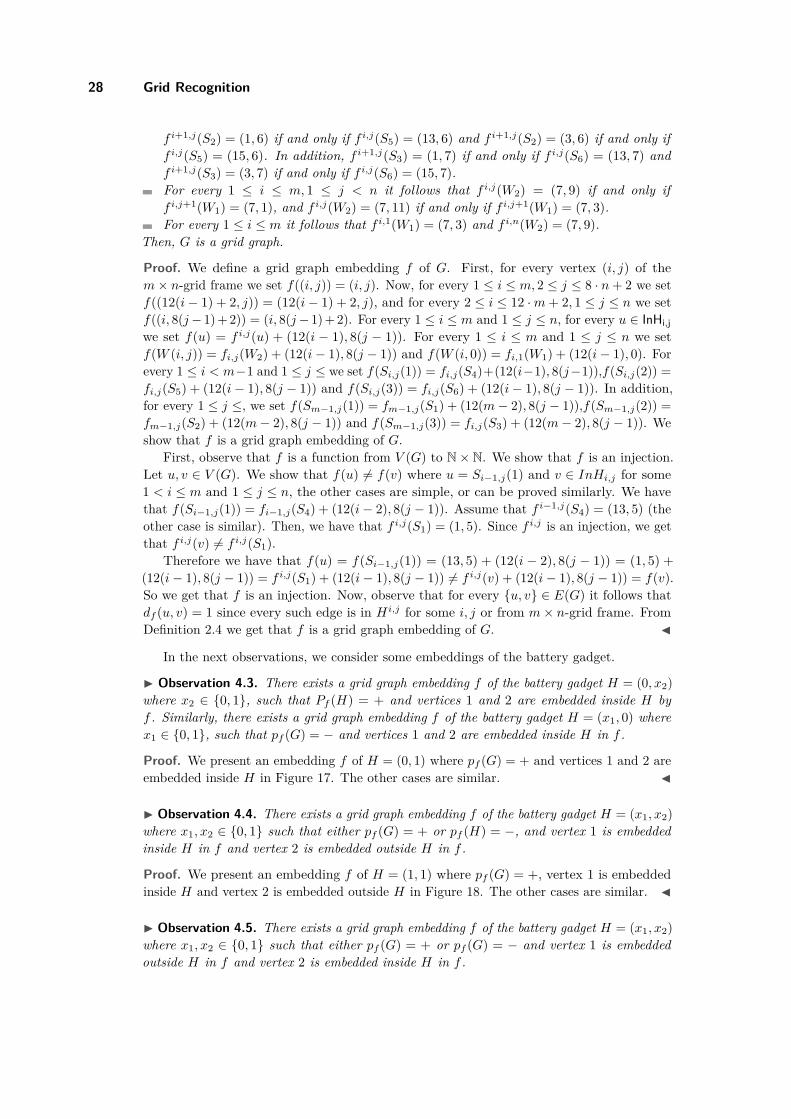
28 Grid Recognition
f i+1,j(S2) = (1, 6) if and only if f i,j(S5) = (13, 6) and f i+1,j(S2) = (3, 6) if and only iff i,j(S5) = (15, 6). In addition, f i+1,j(S3) = (1, 7) if and only if f i,j(S6) = (13, 7) andf i+1,j(S3) = (3, 7) if and only if f i,j(S6) = (15, 7).For every 1 ≤ i ≤ m, 1 ≤ j < n it follows that f i,j(W2) = (7, 9) if and only iff i,j+1(W1) = (7, 1), and f i,j(W2) = (7, 11) if and only if f i,j+1(W1) = (7, 3).For every 1 ≤ i ≤ m it follows that f i,1(W1) = (7, 3) and f i,n(W2) = (7, 9).
Then, G is a grid graph.
Proof. We define a grid graph embedding f of G. First, for every vertex (i, j) of them× n-grid frame we set f((i, j)) = (i, j). Now, for every 1 ≤ i ≤ m, 2 ≤ j ≤ 8 · n+ 2 we setf((12(i− 1) + 2, j)) = (12(i− 1) + 2, j), and for every 2 ≤ i ≤ 12 ·m+ 2, 1 ≤ j ≤ n we setf((i, 8(j− 1) + 2)) = (i, 8(j− 1) + 2). For every 1 ≤ i ≤ m and 1 ≤ j ≤ n, for every u ∈ InHi,jwe set f(u) = f i,j(u) + (12(i − 1), 8(j − 1)). For every 1 ≤ i ≤ m and 1 ≤ j ≤ n we setf(W (i, j)) = fi,j(W2) + (12(i− 1), 8(j − 1)) and f(W (i, 0)) = fi,1(W1) + (12(i− 1), 0). Forevery 1 ≤ i < m−1 and 1 ≤ j ≤ we set f(Si,j(1)) = fi,j(S4)+(12(i−1), 8(j−1)),f(Si,j(2)) =fi,j(S5) + (12(i− 1), 8(j − 1)) and f(Si,j(3)) = fi,j(S6) + (12(i− 1), 8(j − 1)). In addition,for every 1 ≤ j ≤, we set f(Sm−1,j(1)) = fm−1,j(S1) + (12(m− 2), 8(j − 1)),f(Sm−1,j(2)) =fm−1,j(S2) + (12(m− 2), 8(j − 1)) and f(Sm−1,j(3)) = fi,j(S3) + (12(m− 2), 8(j − 1)). Weshow that f is a grid graph embedding of G.
First, observe that f is a function from V (G) to N× N. We show that f is an injection.Let u, v ∈ V (G). We show that f(u) 6= f(v) where u = Si−1,j(1) and v ∈ InHi,j for some1 < i ≤ m and 1 ≤ j ≤ n, the other cases are simple, or can be proved similarly. We havethat f(Si−1,j(1)) = fi−1,j(S4) + (12(i− 2), 8(j − 1)). Assume that f i−1,j(S4) = (13, 5) (theother case is similar). Then, we have that f i,j(S1) = (1, 5). Since f i,j is an injection, we getthat f i,j(v) 6= f i,j(S1).
Therefore we have that f(u) = f(Si−1,j(1)) = (13, 5) + (12(i − 2), 8(j − 1)) = (1, 5) +(12(i− 1), 8(j − 1)) = f i,j(S1) + (12(i− 1), 8(j − 1)) 6= f i,j(v) + (12(i− 1), 8(j − 1)) = f(v).So we get that f is an injection. Now, observe that for every {u, v} ∈ E(G) it follows thatdf (u, v) = 1 since every such edge is in Hi,j for some i, j or from m× n-grid frame. FromDefinition 2.4 we get that f is a grid graph embedding of G. J
In the next observations, we consider some embeddings of the battery gadget.
I Observation 4.3. There exists a grid graph embedding f of the battery gadget H = (0, x2)where x2 ∈ {0, 1}, such that Pf (H) = + and vertices 1 and 2 are embedded inside H byf . Similarly, there exists a grid graph embedding f of the battery gadget H = (x1, 0) wherex1 ∈ {0, 1}, such that pf (G) = − and vertices 1 and 2 are embedded inside H in f .
Proof. We present an embedding f of H = (0, 1) where pf (G) = + and vertices 1 and 2 areembedded inside H in Figure 17. The other cases are similar. J
I Observation 4.4. There exists a grid graph embedding f of the battery gadget H = (x1, x2)where x1, x2 ∈ {0, 1} such that either pf (G) = + or pf (H) = −, and vertex 1 is embeddedinside H in f and vertex 2 is embedded outside H in f .
Proof. We present an embedding f of H = (1, 1) where pf (G) = +, vertex 1 is embeddedinside H and vertex 2 is embedded outside H in Figure 18. The other cases are similar. J
I Observation 4.5. There exists a grid graph embedding f of the battery gadget H = (x1, x2)where x1, x2 ∈ {0, 1} such that either pf (G) = + or pf (G) = − and vertex 1 is embeddedoutside H in f and vertex 2 is embedded inside H in f .
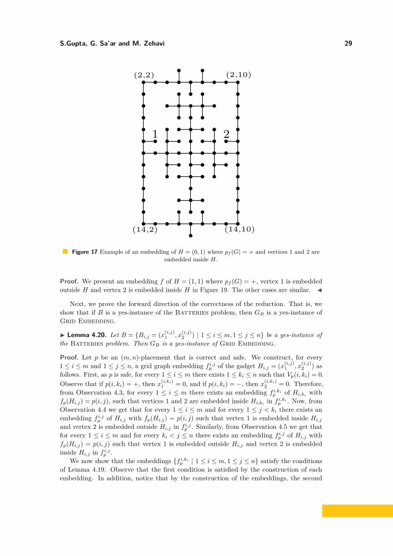
S.Gupta, G. Sa’ar and M. Zehavi 29
1 2
(2,2) (2,10)
(14,2) (14,10)
Figure 17 Example of an embedding of H = (0, 1) where pf (G) = + and vertices 1 and 2 areembedded inside H.
Proof. We present an embedding f of H = (1, 1) where pf (G) = +, vertex 1 is embeddedoutside H and vertex 2 is embedded inside H in Figure 19. The other cases are similar. J
Next, we prove the forward direction of the correctness of the reduction. That is, weshow that if B is a yes-instance of the Batteries problem, then GB is a yes-instance ofGrid Embedding.
I Lemma 4.20. Let B = {Bi,j = (x(i,j)1 , x
(i,j)2 ) | 1 ≤ i ≤ m, 1 ≤ j ≤ n} be a yes-instance of
the Batteries problem. Then GB is a yes-instance of Grid Embedding.
Proof. Let p be an (m,n)-placement that is correct and safe. We construct, for every1 ≤ i ≤ m and 1 ≤ j ≤ n, a grid graph embedding f i,jp of the gadget Hi,j = (x(i,j)
1 , x(i,j)2 ) as
follows. First, as p is safe, for every 1 ≤ i ≤ m there exists 1 ≤ ki ≤ n such that Vp(i, ki) = 0.Observe that if p(i, ki) = +, then x(i,ki)
1 = 0, and if p(i, ki) = −, then x(i,ki)2 = 0. Therefore,
from Observation 4.3, for every 1 ≤ i ≤ m there exists an embedding f i,kip of Hi,ki with
fp(Hi,j) = p(i, j), such that vertices 1 and 2 are embedded inside Hi,kiin f i,ki
p . Now, fromObservation 4.4 we get that for every 1 ≤ i ≤ m and for every 1 ≤ j < ki there exists anembedding f i,jp of Hi,j with fp(Hi,j) = p(i, j) such that vertex 1 is embedded inside Hi,j
and vertex 2 is embedded outside Hi,j in f i,jp . Similarly, from Observation 4.5 we get thatfor every 1 ≤ i ≤ m and for every ki < j ≤ n there exists an embedding f i,jp of Hi,j withfp(Hi,j) = p(i, j) such that vertex 1 is embedded outside Hi,j and vertex 2 is embeddedinside Hi,j in f i,jp .
We now show that the embeddings {f i,kip | 1 ≤ i ≤ m, 1 ≤ j ≤ n} satisfy the conditions
of Lemma 4.19. Observe that the first condition is satisfied by the construction of eachembedding. In addition, notice that by the construction of the embeddings, the second

30 Grid Recognition
1 2
(2,2) (2,10)
(14,2) (14,10)
Figure 18 Example of an embedding of H = (1, 1) where pf (G) = +, vertex 1 is embeddedinside H and vertex 2 is embedded outside H.
condition is satisfied if and only if pf (Hi,j) = pf (Hi+1,j) for every 1 ≤ i < m, 1 ≤ j ≤ n. Let1 ≤ i < m, 1 ≤ j ≤ n. Since p is a correct placement, we get that p(i, j) = p(i+ 1, j), andtherefore pf (Hi,j) = pf (Hi+1,j), so the second condition is satisfied.
If j < ki then vertex 2 of Hi,j is embedded outside Hi,j in f i,jp and vertex 1 of Hi,j+1 isembedded inside Hi,j+1 in f i,j+1
p . If j ≥ ki then vertex 2 of Hi,j is embedded inside Hi,j inf i,jp and vertex 1 of Hi,j+1 is embedded outside Hi,j+1 in f i,j+1
p . Therefore, we get that thethird condition is satisfied.
Observe that for every 1 ≤ i ≤ ki vertex 1 of Hi,j is embedded inside Hi,j in f i,jp . Sinceki ≥ 1 we get that vertex 1 of Hi,1 is embedded inside Hi,1 in f i,1p . Similarly, observe that forevery ki ≤ i ≤ n vertex 2 of Hi,j is embedded inside Hi,j in f i,jp . Since ki ≤ n we get thatvertex 2 of Hi,n is embedded inside Hi,n in f i,np . Therefore we get that the last condition issatisfied. Every condition of Lemma 4.19 is satisfied, therefore GB is a grid graph, and weget that GB is a yes-instance of Grid Embedding. J
So far, we have proved the correctness of our construction. It only remains to show isthat, if GB is a grid graph, then the distance approximation of GB is bounded by a constant.We use the fact that in every grid graph embedding of GB the embedding of the rectanglesof the battery gadgets are fixed, as we saw in Observation 4.12. We show in the next lemmathat if GB is a grid graph with grid graph embedding f , then necessarily af ≤ 234.
I Lemma 4.21. Let B = {Bi,j = (x(i,j)1 , x
(i,j)2 ) | 1 ≤ i ≤ m, 1 ≤ j ≤ n} be an instance of
the Batteries problem. If GB is a grid graph, then for every grid graph embedding f of GBit follows that af ≤ 234.
Proof. Let f be a grid graph embedding of GB. Assume that f((0, 0)) = (0, 0) f((1, 0)) =
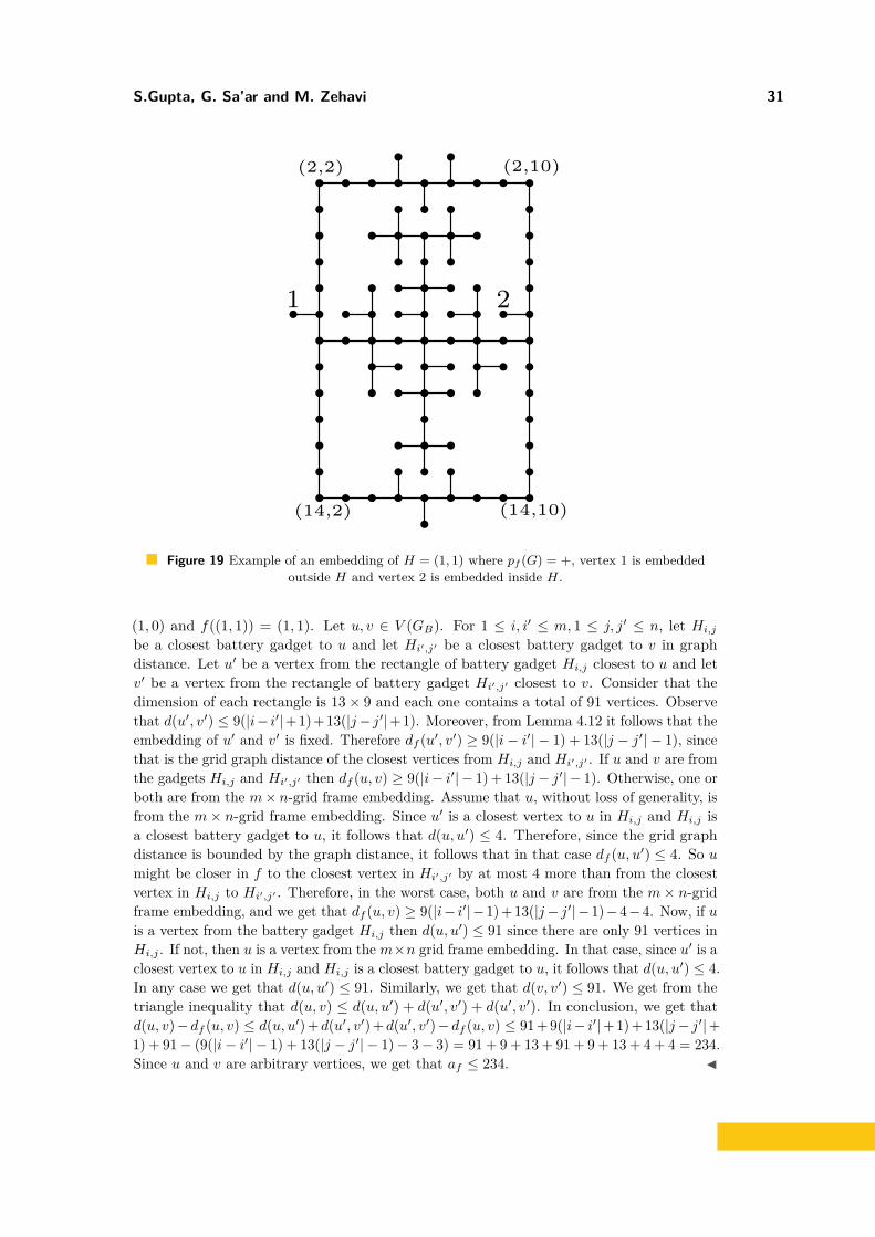
S.Gupta, G. Sa’ar and M. Zehavi 31
1 2
(2,2) (2,10)
(14,2) (14,10)
Figure 19 Example of an embedding of H = (1, 1) where pf (G) = +, vertex 1 is embeddedoutside H and vertex 2 is embedded inside H.
(1, 0) and f((1, 1)) = (1, 1). Let u, v ∈ V (GB). For 1 ≤ i, i′ ≤ m, 1 ≤ j, j′ ≤ n, let Hi,j
be a closest battery gadget to u and let Hi′,j′ be a closest battery gadget to v in graphdistance. Let u′ be a vertex from the rectangle of battery gadget Hi,j closest to u and letv′ be a vertex from the rectangle of battery gadget Hi′,j′ closest to v. Consider that thedimension of each rectangle is 13× 9 and each one contains a total of 91 vertices. Observethat d(u′, v′) ≤ 9(|i− i′|+1)+13(|j− j′|+1). Moreover, from Lemma 4.12 it follows that theembedding of u′ and v′ is fixed. Therefore df (u′, v′) ≥ 9(|i− i′| − 1) + 13(|j − j′| − 1), sincethat is the grid graph distance of the closest vertices from Hi,j and Hi′,j′ . If u and v are fromthe gadgets Hi,j and Hi′,j′ then df (u, v) ≥ 9(|i− i′| − 1) + 13(|j − j′| − 1). Otherwise, one orboth are from the m× n-grid frame embedding. Assume that u, without loss of generality, isfrom the m× n-grid frame embedding. Since u′ is a closest vertex to u in Hi,j and Hi,j isa closest battery gadget to u, it follows that d(u, u′) ≤ 4. Therefore, since the grid graphdistance is bounded by the graph distance, it follows that in that case df (u, u′) ≤ 4. So umight be closer in f to the closest vertex in Hi′,j′ by at most 4 more than from the closestvertex in Hi,j to Hi′,j′ . Therefore, in the worst case, both u and v are from the m× n-gridframe embedding, and we get that df (u, v) ≥ 9(|i− i′|−1) + 13(|j− j′|−1)−4−4. Now, if uis a vertex from the battery gadget Hi,j then d(u, u′) ≤ 91 since there are only 91 vertices inHi,j . If not, then u is a vertex from them×n grid frame embedding. In that case, since u′ is aclosest vertex to u in Hi,j and Hi,j is a closest battery gadget to u, it follows that d(u, u′) ≤ 4.In any case we get that d(u, u′) ≤ 91. Similarly, we get that d(v, v′) ≤ 91. We get from thetriangle inequality that d(u, v) ≤ d(u, u′) + d(u′, v′) + d(u′, v′). In conclusion, we get thatd(u, v)−df (u, v) ≤ d(u, u′) +d(u′, v′) +d(u′, v′)−df (u, v) ≤ 91 + 9(|i− i′|+ 1) + 13(|j− j′|+1) + 91− (9(|i− i′| − 1) + 13(|j − j′| − 1)− 3− 3) = 91 + 9 + 13 + 91 + 9 + 13 + 4 + 4 = 234.Since u and v are arbitrary vertices, we get that af ≤ 234. J
32 Grid Recognition
In the proof of the next lemma, we invoke Observation 4.2, and Lemmas 4.20, 4.18 and4.21 in order to assert the existence of a polynomial reduction from the Batteries problemto Grid Embedding where aG is bounded by a constant.
I Lemma 4.22. There exists a polynomial reduction from the Batteries problem to GridEmbedding where aG is bounded by a constant.
Proof. We show that reduce2 is such a reduction. From Observation 4.2 we get that reduce2 iscomputable in polynomial time. Now, let B = {Bi,j = (x(i,j)
1 , x(i,j)2 ) | 1 ≤ i ≤ m, 1 ≤ j ≤ n}
be an instance of the Batteries problem. If B is a yes-instance of the Batteries problem,then by Lemma 4.20, we get that reduce2(B) = GB is a yes-instance of Grid Embedding.If reduce2(B) = GB is a yes-instance of Grid Embedding, then by Lemma 4.18 B is ayes-instance of the Batteries problem. In addition, by Lemma 4.21 we get that aGB
isbounded by 232 (if GB is a grid graph). This completes the proof. J
In conclusion, in Lemma 4.8 we proved the existence of a polynomial reduction fromSAT to the Batteries problem. In Lemma 4.22 we proved the existence of a polynomialreduction from the Batteries problem to Grid Embedding with aG that is bounded by aconstant. Combining these two results, we conclude the correctness of Theorem 1.4.
I Theorem 1.4. Grid Embedding (and hence also k × r-Grid Embedding) is para-NP-hard parameterized by aG.
4.2 k × r-Grid Embedding is FPT with Respect to k + aG on GeneralGraphs
We present an FPT algorithm with respect to aG and k for the k × r-Grid Embeddingproblem. We remark that we do not need to know the value of aG in advance, in order to useour algorithm, as we iterate over all the potential values for aG. The idea of the algorithm isas follows. We iterate over every possible value for af , from 1 to |V (G)| − 2. For every suchaf , we do the following. We guess one of the leftmost vertices v in the k × r grid, i.e. suchthat fcol(v) = 0. We divide the k× r grid into
⌈r
k+aG
⌉“small rectangles” of size k× (aG + k)
from left to right, except the last rectangle that might be smaller. We find the graph distanceof each vertex from v, i.e. we compute d(v, u) for every u ∈ V . Then, we sort the verticesinto the small rectangles as follows. For each vertex u, we put u in the
⌈d(v,u)k+aG
⌉-th rectangle.
If there is no such rectangle (i.e.⌈d(v,u)k+aG
⌉is too large), then we put u in the last rectangle,
or we can just conclude that we have a no-instance.Afterwards, we show that in every k × r grid graph embedding f of G with af = aG
where v is one of the leftmost vertices, every u is embedded either in its sorted rectangle orthe previous one. An intuition for this is similar to our former argument about the structureof a grid graph embedding with distance approximation af : On the one hand, the vertex ucannot be embedded into a farther rectangle as its shortest path (or paths) from v cannotbe embedded in that case; on other hand, if u is embedded into a closer rectangle, then theembedding does not respect the distance approximation. We will prove this claim formally;here we just give an overview. Then, after we know the approximate “location” of eachvertex, we try to find a k × r grid graph embedding of G.
We denote the set of vertices located between the s-th column and the t-th column in ak× r grid graph embedding f of G by Cf (s, t), i.e. Cf (s, t) = {u ∈ V : s ≤ fcol(u) ≤ t}. Inaddition, for any two integers 0 ≤ s ≤ t, we denote the set of vertices with graph distance

S.Gupta, G. Sa’ar and M. Zehavi 33
at least s and at most t from v by Dv(s, t), i.e. Dv(s, t) = {u ∈ V | s ≤ d(v, u) ≤ t}. SeeFigure 20.
d(v, u) ∈[0, k + af
)
d(v, u) ∈[k + af , 2(k + af )
)
d(v, u) ∈[(dr/(k + af )e − 1)(k + afs), r
]v
Figure 20 The partition of the k × r grid into small rectangles and the approximate position ofany vertex u with respect to v.
I Lemma 4.23. Let G = (V,E) be a k×r grid graph, and let f be a k×r grid graph embeddingof G. Let v ∈ V such that fcol(v) = 0. Let u ∈ V . Then, u ∈ Cf (d(u, v) − af − k, d(u, v))and u ∈ Dv(fcol(u), fcol(u) + af + k).
Proof. First, we show that u ∈ Cf (d(u, v)−af−k, d(u, v)). Observe that for every u ∈ V , wehave that d(u, v) ≥ df (u, v) ≥ |fcol(u)− fcol(v)| = |fcol(u)− 0| = fcol(u). In addition, noticethat |frow(u)− frow(v)| ≤ k. Therefore, we get that df (u, v) = |fcol(u)− fcol(v)|+ |frow(u)−frow(v)| ≤ |fcol(u) − fcol(v)| + k = fcol(u) + k. Now, we have that d(u, v) − df (u, v) ≤ af .Therefore, d(u, v)−fcol(u)−k ≤ d(u, v)−df (u, v) ≤ af . Combining these two inequalities, weget that d(u, v)−af −k ≤ fcol(u) ≤ d(u, v). So we have that u ∈ Cf (d(u, v)−af −k, d(u, v)).
Second, we show that u ∈ Dv(fcol(u), fcol(u) + af + k). We have that af is the distanceapproximation of f , therefore we get that d(u, v) ≤ df (u, v) + af . We saw that df (u, v) ≤fcol(u) + k. Therefore we get that d(u, v) ≤ fcol(u) + af + k. In addition, we also sawthat d(u, v) ≥ fcol(u). Combining these two inequalities, we get that fcol(u) ≤ d(u, v) ≤fcol(u) + af + k. So we have that u ∈ Dv(fcol(u), fcol(u) + af + k). J
In Lemma 4.23 we assume that there exists a vertex v with fcol(v) = 0. Notice that forevery k × r grid graph embedding f of G, we can construct a k × r grid graph embeddingf ′ of G with af ′ = af and with such a vertex v: indeed, we can simply define f ′(u) =(frow(u), fcol(u)−m) where m = Minv∈V {fcol(v)}; then, observe that f ′ is a k× r grid graphembedding of G with af ′ = af and with Minv∈V {f ′col(v)} = 0. We state this in the nextobservation.
I Observation 4.6. Let G = (V,E) be a k × r grid graph, and let f be a k × r grid graphembedding of G. Then, there exists a k × r grid graph embedding f ′ of G with af ′ = af andMinv∈V {f ′col(v)} = 0.
Now we further discuss the idea of the algorithm. We use dynamic programming inorder to find a k × r grid graph embedding of G in the following manner. First, we get theapproximate location for each vertex as explained earlier. Then, starting from left to right,we try to find an embedding for each of the “small rectangles” that agrees with one of theembeddings for the previous one. In order to do this, we only need to know which verticesfrom the current rectangle we have already embedded in the previous one, and what is theembedding in the last column. Notice that, each time, we need to store information whosesize depends only on r and aG. In this way, after the last iteration corresponding to the lastrectangle, we can get the embedding of G (if such exists), or conclude that there is no suchan embedding.
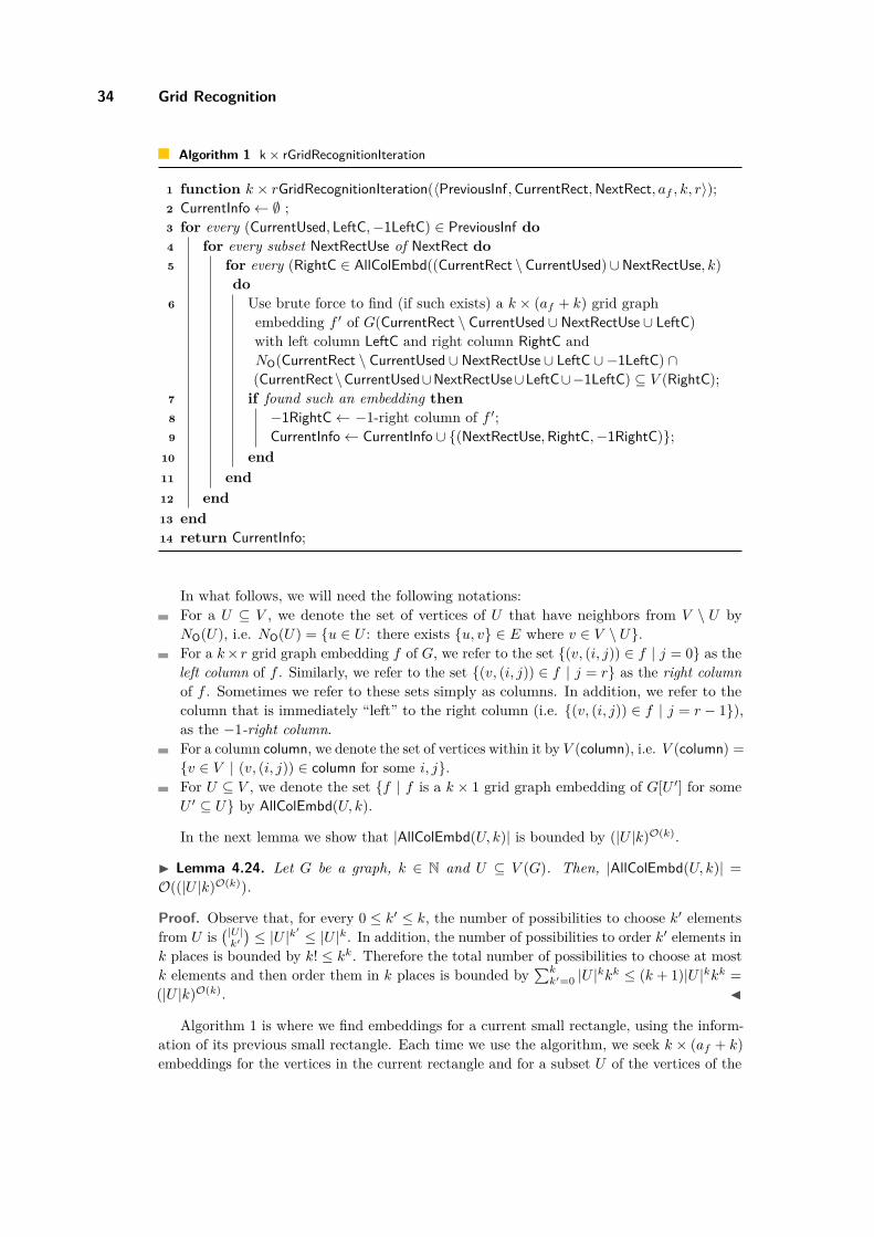
34 Grid Recognition
Algorithm 1 k× rGridRecognitionIteration
1 function k × rGridRecognitionIteration(〈PreviousInf,CurrentRect,NextRect, af , k, r〉);2 CurrentInfo← ∅ ;3 for every (CurrentUsed, LeftC,−1LeftC) ∈ PreviousInf do4 for every subset NextRectUse of NextRect do5 for every (RightC ∈ AllColEmbd((CurrentRect \CurrentUsed)∪NextRectUse, k)
do6 Use brute force to find (if such exists) a k × (af + k) grid graph
embedding f ′ of G(CurrentRect \ CurrentUsed ∪ NextRectUse ∪ LeftC)with left column LeftC and right column RightC andNO(CurrentRect \ CurrentUsed ∪ NextRectUse ∪ LeftC ∪ −1LeftC) ∩(CurrentRect\CurrentUsed∪NextRectUse∪LeftC∪−1LeftC) ⊆ V (RightC);
7 if found such an embedding then8 −1RightC← −1-right column of f ′;9 CurrentInfo← CurrentInfo ∪ {(NextRectUse,RightC,−1RightC)};
10 end11 end12 end13 end14 return CurrentInfo;
In what follows, we will need the following notations:For a U ⊆ V , we denote the set of vertices of U that have neighbors from V \ U byNO(U), i.e. NO(U) = {u ∈ U : there exists {u, v} ∈ E where v ∈ V \ U}.For a k× r grid graph embedding f of G, we refer to the set {(v, (i, j)) ∈ f | j = 0} as theleft column of f . Similarly, we refer to the set {(v, (i, j)) ∈ f | j = r} as the right columnof f . Sometimes we refer to these sets simply as columns. In addition, we refer to thecolumn that is immediately “left” to the right column (i.e. {(v, (i, j)) ∈ f | j = r − 1}),as the −1-right column.For a column column, we denote the set of vertices within it by V (column), i.e. V (column) ={v ∈ V | (v, (i, j)) ∈ column for some i, j}.For U ⊆ V , we denote the set {f | f is a k × 1 grid graph embedding of G[U ′] for someU ′ ⊆ U} by AllColEmbd(U, k).
In the next lemma we show that |AllColEmbd(U, k)| is bounded by (|U |k)O(k).
I Lemma 4.24. Let G be a graph, k ∈ N and U ⊆ V (G). Then, |AllColEmbd(U, k)| =O((|U |k)O(k)).
Proof. Observe that, for every 0 ≤ k′ ≤ k, the number of possibilities to choose k′ elementsfrom U is
(|U |k′
)≤ |U |k′ ≤ |U |k. In addition, the number of possibilities to order k′ elements in
k places is bounded by k! ≤ kk. Therefore the total number of possibilities to choose at mostk elements and then order them in k places is bounded by
∑kk′=0 |U |kkk ≤ (k + 1)|U |kkk =
(|U |k)O(k). J
Algorithm 1 is where we find embeddings for a current small rectangle, using the inform-ation of its previous small rectangle. Each time we use the algorithm, we seek k × (af + k)embeddings for the vertices in the current rectangle and for a subset U of the vertices of the
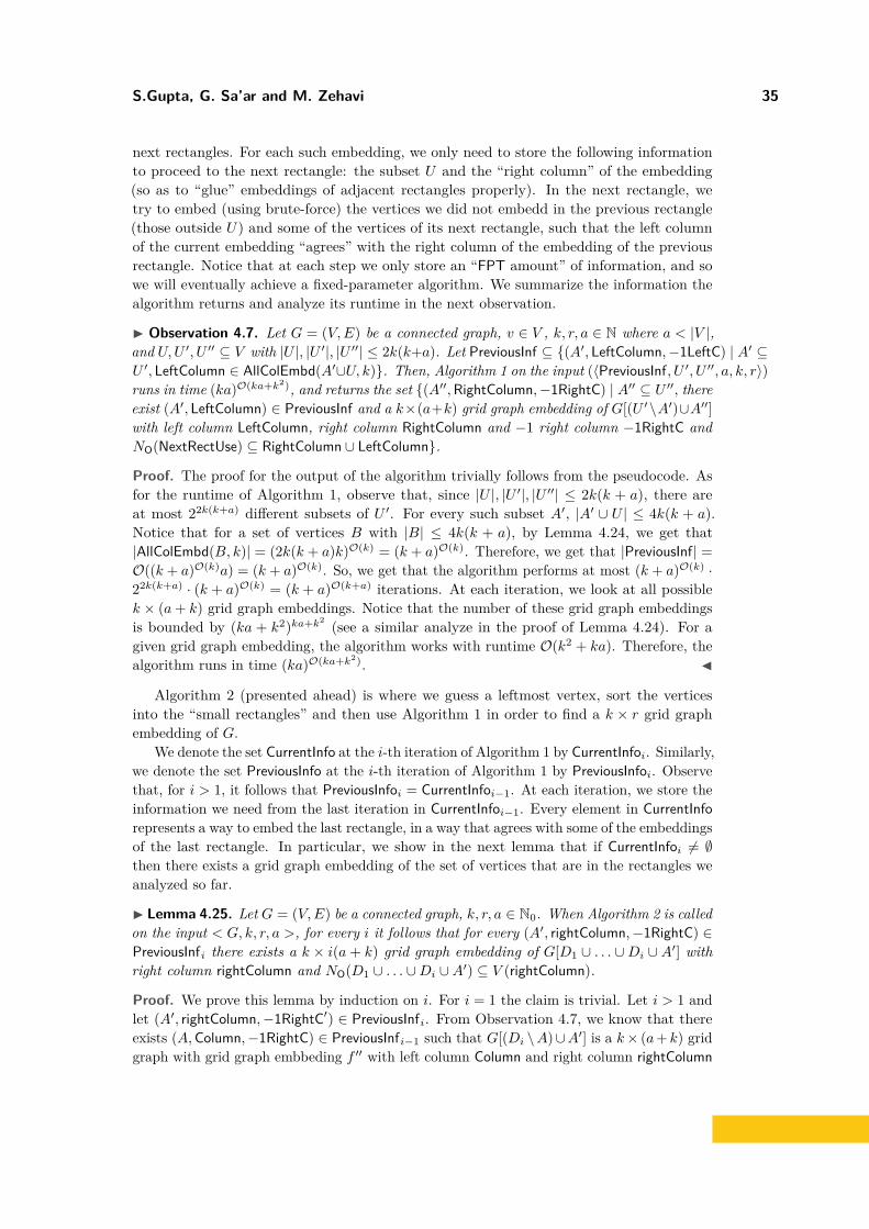
S.Gupta, G. Sa’ar and M. Zehavi 35
next rectangles. For each such embedding, we only need to store the following informationto proceed to the next rectangle: the subset U and the “right column” of the embedding(so as to “glue” embeddings of adjacent rectangles properly). In the next rectangle, wetry to embed (using brute-force) the vertices we did not embedd in the previous rectangle(those outside U) and some of the vertices of its next rectangle, such that the left columnof the current embedding “agrees” with the right column of the embedding of the previousrectangle. Notice that at each step we only store an “FPT amount” of information, and sowe will eventually achieve a fixed-parameter algorithm. We summarize the information thealgorithm returns and analyze its runtime in the next observation.
I Observation 4.7. Let G = (V,E) be a connected graph, v ∈ V , k, r, a ∈ N where a < |V |,and U,U ′, U ′′ ⊆ V with |U |, |U ′|, |U ′′| ≤ 2k(k+a). Let PreviousInf ⊆ {(A′, LeftColumn,−1LeftC) | A′ ⊆U ′, LeftColumn ∈ AllColEmbd(A′∪U, k)}. Then, Algorithm 1 on the input (〈PreviousInf, U ′, U ′′, a, k, r〉)runs in time (ka)O(ka+k2), and returns the set {(A′′,RightColumn,−1RightC) | A′′ ⊆ U ′′, thereexist (A′, LeftColumn) ∈ PreviousInf and a k×(a+k) grid graph embedding of G[(U ′\A′)∪A′′]with left column LeftColumn, right column RightColumn and −1 right column −1RightC andNO(NextRectUse) ⊆ RightColumn ∪ LeftColumn}.
Proof. The proof for the output of the algorithm trivially follows from the pseudocode. Asfor the runtime of Algorithm 1, observe that, since |U |, |U ′|, |U ′′| ≤ 2k(k + a), there areat most 22k(k+a) different subsets of U ′. For every such subset A′, |A′ ∪ U | ≤ 4k(k + a).Notice that for a set of vertices B with |B| ≤ 4k(k + a), by Lemma 4.24, we get that|AllColEmbd(B, k)| = (2k(k + a)k)O(k) = (k + a)O(k). Therefore, we get that |PreviousInf| =O((k + a)O(k)a) = (k + a)O(k). So, we get that the algorithm performs at most (k + a)O(k) ·22k(k+a) · (k + a)O(k) = (k + a)O(k+a) iterations. At each iteration, we look at all possiblek × (a+ k) grid graph embeddings. Notice that the number of these grid graph embeddingsis bounded by (ka + k2)ka+k2 (see a similar analyze in the proof of Lemma 4.24). For agiven grid graph embedding, the algorithm works with runtime O(k2 + ka). Therefore, thealgorithm runs in time (ka)O(ka+k2). J
Algorithm 2 (presented ahead) is where we guess a leftmost vertex, sort the verticesinto the “small rectangles” and then use Algorithm 1 in order to find a k × r grid graphembedding of G.
We denote the set CurrentInfo at the i-th iteration of Algorithm 1 by CurrentInfoi. Similarly,we denote the set PreviousInfo at the i-th iteration of Algorithm 1 by PreviousInfoi. Observethat, for i > 1, it follows that PreviousInfoi = CurrentInfoi−1. At each iteration, we store theinformation we need from the last iteration in CurrentInfoi−1. Every element in CurrentInforepresents a way to embed the last rectangle, in a way that agrees with some of the embeddingsof the last rectangle. In particular, we show in the next lemma that if CurrentInfoi 6= ∅then there exists a grid graph embedding of the set of vertices that are in the rectangles weanalyzed so far.
I Lemma 4.25. Let G = (V,E) be a connected graph, k, r, a ∈ N0. When Algorithm 2 is calledon the input < G, k, r, a >, for every i it follows that for every (A′, rightColumn,−1RightC) ∈PreviousInfi there exists a k × i(a+ k) grid graph embedding of G[D1 ∪ . . . ∪Di ∪ A′] withright column rightColumn and NO(D1 ∪ . . . ∪Di ∪A′) ⊆ V (rightColumn).
Proof. We prove this lemma by induction on i. For i = 1 the claim is trivial. Let i > 1 andlet (A′, rightColumn,−1RightC′) ∈ PreviousInfi. From Observation 4.7, we know that thereexists (A,Column,−1RightC) ∈ PreviousInfi−1 such that G[(Di \A)∪A′] is a k× (a+ k) gridgraph with grid graph embbeding f ′′ with left column Column and right column rightColumn

36 Grid Recognition
Algorithm 2 k× rGridRecognitionwithaf
1 function k × rGridRecognitionwithaf (〈G = (V,E), k, r, af 〉);2 for every v ∈ V do3 Find d(u, v) for every u ∈ V ;4 if there exists u ∈ V with d(u, v)− af > r then5 return 〈G, k, r, af 〉 is a no-instance;6 end7 for every i ∈ [
⌈r
k+aG
⌉] + 1 do
8 Create an empty set Di;9 end
10 for every u ∈ V do11 i←
⌊d(u,v)k+af
⌋;
12 Di ← Di ∪ {u};13 end14 if there exists Di with |Di| > 2k(k + af ) then15 Break;16 end17 Let j be the maximum such that Dj 6= ∅;18 CurrentInfo← (∅, emptyColumn);19 i← 0 while CurrentInfo 6= ∅ and i ≤ j + 1 do20 CurrentInfo← k × rGridRecognitionIteration(〈CurrentInfo, Di, Di+1, af , k, r〉);21 i← i+ 1;22 end23 if CurrentInfo = ∅ then24 Break;25 end26 return 〈G, k, r, af 〉 is a yes-instance;27 end28 return 〈G, k, r, af 〉 is a no-instance;
and NO((Di \ A) ∪ A′ ∪ −1RightC) ∩ ((Di \ A) ∪ A′∪) ⊆ rightColumn. From the inductionhypothesis, we get that there exists a k × (i − 1)(a + k) grid graph embedding f ′ ofG[D1∪ . . .∪Di−1∪A] with right column Column and NO(D1∪ . . .∪Di−1∪A) ⊆ V (Column).We can assume that f ′′col(Column) = 0, and f ′col(v) = 0 for some vertex v. Observe that(Di − A ∪ A′) ∩ (D1 ∪ . . . ∪Di−1 ∪ A) = V (Column). We define a k × i(a + k) grid graphembedding f of G[D1 ∪ . . . ∪ Di ∪ A′]. If v ∈ (D1 ∪ . . . ∪ Di−1 ∪ A), then f(v) = f ′(v);otherwise f(v) = (f ′′row(v), f ′′col(v) + f ′′col(Column)). Observe that f is an injection. For{u, v} ∈ E(G[D1 ∪ . . .∪Di ∪A′]), if u, v ∈ D1 ∪ . . .∪Di−1 ∪A then df (u, v) = 1 since f ′ is ak× i(a+ k) grid graph embedding of G[D1 ∪ . . .∪Di−1 ∪A]. Similarly, if u, v ∈ Di −A∪A′then df (u, v) = 1 since f ′′ is a k × (a+ k) grid graph embedding of G[Di −A ∪A′]. Assumethat u ∈ D1∪ . . .∪Di−1∪A and v ∈ Di−A∪A′. Then, u ∈ V (Column) ⊆ D1∪ . . .∪Di−1∪A,so df (u, v) = 1 since f ′ is a k× i(a+k) grid graph embedding of G[D1∪ . . .∪Di−1∪A]. Now,let v ∈ NO(D1 ∪ . . .∪Di ∪A′). If v ∈ D1 ∪ . . .∪Di−1 ∪A then v ∈ NO(D1 ∪ . . .∪Di−1 ∪A).Therefore, we have that v ∈ V (Column). Since v /∈ V (rightColumn), we have that v /∈NO((Di \ A) ∪ A′ ∪ −1RightC) ∩ ((Di \ A) ∪ A′), therefore v /∈ NO(D1 ∪ . . . ∪ Di ∪ A′), a
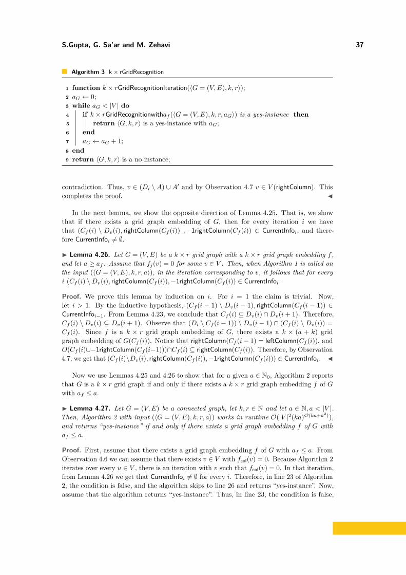
S.Gupta, G. Sa’ar and M. Zehavi 37
Algorithm 3 k× rGridRecognition
1 function k × rGridRecognitionIteration(〈G = (V,E), k, r〉);2 aG ← 0;3 while aG < |V | do4 if k × rGridRecognitionwithaf (〈G = (V,E), k, r, aG〉) is a yes-instance then5 return 〈G, k, r〉 is a yes-instance with aG;6 end7 aG ← aG + 1;8 end9 return 〈G, k, r〉 is a no-instance;
contradiction. Thus, v ∈ (Di \ A) ∪ A′ and by Observation 4.7 v ∈ V (rightColumn). Thiscompletes the proof. J
In the next lemma, we show the opposite direction of Lemma 4.25. That is, we showthat if there exists a grid graph embedding of G, then for every iteration i we havethat (Cf (i) \ Dv(i), rightColumn(Cf (i)) ,−1rightColumn(Cf (i)) ∈ CurrentInfoi, and there-fore CurrentInfoi 6= ∅.
I Lemma 4.26. Let G = (V,E) be a k × r grid graph with a k × r grid graph embedding f ,and let a ≥ af . Assume that fj(v) = 0 for some v ∈ V . Then, when Algorithm 1 is called onthe input (〈G = (V,E), k, r, a〉), in the iteration corresponding to v, it follows that for everyi (Cf (i) \Dv(i), rightColumn(Cf (i)),−1rightColumn(Cf (i)) ∈ CurrentInfoi.
Proof. We prove this lemma by induction on i. For i = 1 the claim is trivial. Now,let i > 1. By the inductive hypothesis, (Cf (i − 1) \ Dv(i − 1), rightColumn(Cf (i − 1)) ∈CurrentInfoi−1. From Lemma 4.23, we conclude that Cf (i) ⊆ Dv(i) ∩Dv(i+ 1). Therefore,Cf (i) \ Dv(i) ⊆ Dv(i + 1). Observe that (Di \ Cf (i − 1)) \ Dv(i − 1) ∩ (Cf (i) \ Dv(i)) =Cf (i). Since f is a k × r grid graph embedding of G, there exists a k × (a + k) gridgraph embedding of G(Cf (i)). Notice that rightColumn(Cf (i− 1) = leftColumn(Cf (i)), andO(Cf (i)∪−1rightColumn(Cf (i−1)))∩Cf (i) ⊆ rightColumn(Cf (i)). Therefore, by Observation4.7, we get that (Cf (i)\Dv(i), rightColumn(Cf (i)),−1rightColumn(Cf (i))) ∈ CurrentInfoi. J
Now we use Lemmas 4.25 and 4.26 to show that for a given a ∈ N0, Algorithm 2 reportsthat G is a k × r grid graph if and only if there exists a k × r grid graph embedding f of Gwith af ≤ a.
I Lemma 4.27. Let G = (V,E) be a connected graph, let k, r ∈ N and let a ∈ N, a < |V |.Then, Algorithm 2 with input (〈G = (V,E), k, r, a〉) works in runtime O(|V |2(ka)O(ka+k2)),and returns “yes-instance” if and only if there exists a grid graph embedding f of G withaf ≤ a.
Proof. First, assume that there exists a grid graph embedding f of G with af ≤ a. FromObservation 4.6 we can assume that there exists v ∈ V with fcol(v) = 0. Because Algorithm 2iterates over every u ∈ V , there is an iteration with v such that fcol(v) = 0. In that iteration,from Lemma 4.26 we get that CurrentInfoi 6= ∅ for every i. Therefore, in line 23 of Algorithm2, the condition is false, and the algorithm skips to line 26 and returns “yes-instance”. Now,assume that the algorithm returns “yes-instance”. Thus, in line 23, the condition is false,

38 Grid Recognition
so we get that CurrentInfoj+1 6= ∅. From Lemma 4.25, we get that there exists a k × r gridgraph embedding f of G with af ≤ a.
As for the runtime, for a chosen vertex v ∈ V in line 2 of Algorithm 2, computing d(u, v)in line 2 for every u ∈ V can be done with runtime O(|V |2). From line 4, we get that unlessthe iteration breaks, |Di| ≤ 2k(k + af ). Therefore, by Observation 4.7, each iteration inthe while loop in line 19 takes runtime O(ka)O(ka+k2), and there are at most r ≤ |V | suchiterations. The other operations in the algorithm can be done with runtime O(|V |). Inconclusion, we get that the algorithm works with runtime O(|V |2(ka)O(ka+k2)) and returns“yes-instance” if and only if there exists a grid graph embedding f of G with af ≤ a. J
Finally, we are ready to show that Algorithm 3 solves the k × r-Grid Embeddingproblem with FPT runtime with respect to r + aG. The algorithm, in every iteration,activates Algorithm 2 with a larger af than before. If G is a k×r grid graph, then by Lemma4.27, Algorithm 2 will report this in the aG-th iteration. Otherwise, in every iteration thealgorithms fails to prove that G is a k × r grid graph, and it will report that (G, k, r) is ano-instance.
I Lemma 4.28. Let G = (V,E) be a connected graph, and k, r ∈ N. Then, Algorithm 3 withinput 〈G = (V,E), k, r〉 runs in time O(|V |2(kaG)O(kaG+k2)) and returns “yes-instance” ifand only if G is a k × r grid graph.
Proof. First, notice that every iteration in the while loop in line 3 of Algorithm 3 runsAlgorithm 2 on the input (〈G = (V,E), k, r, aG〉). Therefore, by Lemma 4.27, the aG-thiteration runs in time O(|V |2(kaG)O(kaG+k2)). Assume that G is a k × r grid graph. Then,there exists a k × r grid graph embedding f of G with af = aG. Therefore, in the af -thiteration the algorithm activates Algorithm 2 on the input (〈G = (V,E), k, r, af 〉), and, byLemma 4.27, returns yes-instance. Therefore, in that case, the algorithm runs af iterations,where each iteration runs in time at most O(|V |2(kaf )O(kaf +k2)). Therefore the totalruntime is af · O(|V |2(kaf )O(kaf +k2)) = O(|V |2(kaf )O(kaf +k2)) = O(|V |2(kaG)O(kaG+k2)).Now, assume that Algorithm 3 returns “no-instance”. Then, for every 0 ≤ aG ≤ |V |, itfollows that Algorithm 2 returns “no-instance”. Thus, by Lemma 3, there does not exist ak × r grid graph embedding f of G with 0 ≤ af ≤ |V |. By Observation 2.4, we get that Gis not a k × r grid graph. Notice that, in this case, we get that aG = |V |. Furthermore,in that case, the algorithm runs |V | iterations, where each iteration runs in time at mostO(|V |2(k|V |)O(k|V |+k2)). Therefore, the total runtime is |V | · O(|V |2(k|V |)O(k|V |+k2)) =aG · O(|V |2(kaG)O(kaG+k2)) = O(|V |2(kaG)O(kaG+k2)). In conclusion, we get that Algorithm3 on the input 〈G = (V,E), k, r〉 runs in time O(|V |2(kaG)O(kaG+k2)) and returns “yes-instance” if and only if G is a k × r grid graph problem. J
Having proved that Algorithm 3 solves the k × r-Grid Embeddingproblem with FPTruntime, we can conclude the correctness of Theorem 1.5.
I Theorem 1.5. k × r-Grid Embedding is FPT parameterized by aG + k.
4.3 k × r-Grid Embedding Is FPT with Respect to aG on TreesLet T be a tree that is a grid graph, with a grid graph embedding f ′ of T . First, we showthat f ′ has a special structure, that depends on af ′ . We begin with a simple example. Forthis purpose, we present a way to define “directions” in a given grid graph embedding. Let Gbe a connected grid graph, with grid graph embedding f of G, and let {u, v} ∈ E(G) be anedge. We say that {u, v} is directed up in f if frow(v) = frow(u) + 1. Similarly, we say that

S.Gupta, G. Sa’ar and M. Zehavi 39
{u, v} is directed down in f , directed right in f , or directed left in f , if frow(v) = frow(u)− 1,fcol(v) = fcol(u) + 1, or fcol(v) = fcol(u)− 1, correspondingly. Notice that, since f is a gridgraph embedding of G, exactly one of these four options is valid.
It is easy to see that every path is a grid graph. Consider a path P = (v1, v2, . . . v`), where` ≥ 2, and a grid graph embedding f of P with af=0. Without loss of generality, assumethat {v1, v2} is directed up in f . Assume that there exists 2 ≤ t ≤ ` such that {vt−1, vt} isnot directed up in f , and let s be the minimum integer that satisfies this condition. Because{vs−2, vs−1} is directed up, notice that {vs−1, vs} cannot be directed down. Assume that{vs−1, vs} is directed right in f . We show that, for every 1 ≤ t ≤ `− 1, {vt, vt+1} is directedup or right in f . An intuition for that is, every time we “go forward” in the path, we increasethe graph distance between the starting vertex and the current vertex by one, and thereforewe need to increase the grid graph embedding by one, otherwise we get that af > 0. Thus,we cannot “go back”. For a general grid graph embedding f of P , we show that there areat most two “main directions” in which we move from each vi to vi+1, and we cannot goin the other directions, more then af times. Observe that given a general connected gridgraph G, and a path P = (v1, v2, . . . v`), vi ∈ V (G), such that P is a shortest path betweenv1 to v`, we can argue the same claim. Therefore, we conclude that, given a tree T that is agrid graph, with grid graph embedding f , for every path P ⊆ T it follows that there are two“main directions” in which the path “moves”. We start by proving this idea. Towards that,we define the terms of “directions”:
I Definition 4.29 (Grid Direction for Edges). Let G be a connected grid graph, withgrid graph embedding f of G. Let {u, v} ∈ E(G). We say that the grid direction of {u, v} in fis up, down, right, or left, if frow(v) = frow(u) + 1, frow(v) = frow(u)− 1, fcol(v) = fcol(u) + 1,or fcol(v) = fcol(u) − 1, correspondingly. We refer to up, down, right and left as directions.We denote the set of directions by dir, i.e. dir = {up, down, right, left}.
We refer to the up and down directions as vertical directions, and to the right and leftdirections as horizontal directions.
Now we prove the claim in the example we saw before. Let T be a tree, and let f be agrid graph embedding of T . For a simple path P = (v1, . . . , v`), we consider the direction ofthe edges {{vi, vi+1} | 1 ≤ i ≤ `− 1}. For a set of one or more directions ∆ ⊆ dir, we saythat P moves mainly in directions ∆ in f or P moves in directions ∆ in f if the followingcondition is satisfied: The number of edges with direction d′ /∈ ∆ in f is equal or less thanaf + 1. Sometimes, we only refer to the number of direction in ∆. In the next lemma, weshow that P moves in two directions, one vertical and one horizontal.
I Lemma 4.30. Let T be a tree that is a grid graph, with a grid graph embedding f ofT . Then, every simple path moves in f in at most one vertical direction and at most onehorizontal directions.
Proof. Let P = (u,w1 . . . , w`, v) be a simple path. T is a tree, therefore, P is a shortestpath, from u to v, so |P | − 1 = d(u, v). Assume towards a contradiction, without loss ofgenerality, that P moves in two vertical directions more than af + 1 steps. Observe thatdf (u, v) = |fcol(u)− fcol(v)|+ |frow(u)− frow(v)|. Denote the number of edges in P directedup in f , and the number of edges in P directed down in f , by DU (f, P ) and DD(f, P ),correspondingly. Notice that fcol(v) = fcol(u) +DU (f, P )−DD(f, P ). Since there at leastaf + 1 edges in P directed up, and at least af + 1 edges in P directed down, it follows thatdf (u, v) ≤ |P | − af − 1 = d(u, v)− af − 1. Therefore, we get that d(u, v)− df (u, v) ≥ af + 1.This is a contradiction to the definition of af . J
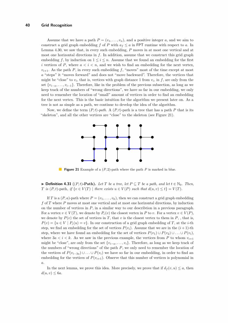
40 Grid Recognition
Assume that we have a path P = (v1, . . . , vn), and a positive integer a, and we aim toconstruct a grid graph embedding f of P with af ≤ a in FPT runtime with respect to a. InLemma 4.30, we saw that, in every such embedding, P moves in at most one vertical and atmost one horizontal directions in f . In addition, assume that we construct this grid graphembedding f , by induction on 1 ≤ i ≤ n. Assume that we found an embedding for the firsti vertices of P , where a < i < n, and we wish to find an embedding for the next vertex,vi+1. As the path P , in every such embedding f , “moves” most of the time except at mosta “steps” it “moves forward” and does not “move backward”. Therefore, the vertices thatmight be “close” to vi, that is, vertices with graph distance 1 from vi, in f , are only from theset {vi−a, . . . , vi−1}. Therefore, like in the problem of the previous subsection, as long as wekeep track of the numbers of “wrong directions”, we have so far in our embedding, we onlyneed to remember the location of “small” amount of vertices in order to find an embeddingfor the next vertex. This is the basic intuition for the algorithm we present later on. As atree is not as simple as a path, we continue to develop the idea of the algorithm.
Now, we define the term (P, t)-path. A (P, t)-path is a tree that has a path P that is its“skeleton”, and all the other vertices are “close” to the skeleton (see Figure 21).
Figure 21 Example of a (P, 2)-path where the path P is marked in blue.
I Definition 4.31 ((P, t)-Path). Let T be a tree, let P ⊆ T be a path, and let t ∈ N0. Then,T is (P, t)-path, if {v ∈ V (T ) | there exists u ∈ V (P ) such that d(u, v) ≤ t} = V (T ).
If T is a (P, a)-path where P = (v1, . . . , vk), then we can construct a grid graph embeddingf of T where P moves at most one vertical and at most one horizontal directions, by inductionon the number of vertices in P , in a similar way to our describtion in a previous paragraph.For a vertex v ∈ V (T ), we denote by Pc(v) the closest vertex in P to v. For a vertex v ∈ V (P ),we denote by P (v) the set of vertices in T , that v is the closest vertex to them in P , , that is,P (v) = {u ∈ V | Pc(u) = v}. In our construction of a grid graph embedding of T , at the i-thstep, we find an embedding for the set of vertices P (vi). Assume that we are in the (i+ 1)-thstep, where we have found an embedding for the set of vertices P (v1) ∪ P (v2) ∪ . . . ∪ P (vi),where 3a < i < k. As we saw in the previous example, the vertices from P to whom vi+1might be “close”, are only from the set {vi−a, . . . , vi}. Therefore, as long as we keep track ofthe numbers of “wrong directions” of the path P , we only need to remember the location ofthe vertices of P (vi−3a) ∪ . . . ∪ P (vi) we have so far in our embedding, in order to find anembedding for the vertices of P (vi+1). Observe that this number of vertices is polynomial ina.
In the next lemma, we prove this idea. More precisely, we prove that if df (v, u) ≤ a, thend(u, v) ≤ 6a.

S.Gupta, G. Sa’ar and M. Zehavi 41
Figure 22 Example of a 5-one-split vertex (in red) and a 3-double-split vertices (in orange).
I Lemma 4.32. Let T be a (P, t)-path that is a grid graph, with grid graph embedding f ofT , such that P moves in two directions in f except for at most t edges. Then, for everyv, u ∈ V such that df (v, u) ≤ t, it follows that d(u, v) ≤ 6t.
Proof. Let u, v ∈ V (T ) such that df (v, u) ≤ t. Let u′ = Pc(u) and v′ = Pc(v). Noticethat, because T is a (P, t)-path, it follows that d(u, u′) ≤ t and d(u, u′) ≤ t. Therefore,it follows that df (u, u′) ≤ t, and df (v, v′) ≤ t. Now, because P moves in at most twodirections in f , it follows that df (v′, u′) ≥ d(u′, v′) − t. Therefore, we get that d(v, u) ≤d(v, v′) + d(v′, u′) + d(u′, u) ≤ t+ df (u′, v′) + t+ t ≤ df (v, v′) + df (v, u) + df (u′, u) + 3t ≤d(v, v′) + df (v, u) + d(u′, u) + 3t ≤ t+ t+ t+ 3t = 6t. J
Obviously, for a given tree T and a positive integer a, it is not sure that there existsa simple path P , such that T is a (P, a)-path. In order to find such a P , we need P to“get inside” every “big” subtree. Assume that T has a vertex with three or four neighborsthat are “attached” to some “big” subtrees of T . Since every simple path can “get inside”at most two of them, we cannot find such a P . We call these vertices a-split vertices. Ana-one-split vertex is a vertex that is “connected” to exactly three “big” subtrees, that is, eachsubtree with at least a vertices. An a-double-split vertex is a vertex that is “connected” tofour “big” subtrees, that is, each subtree with at least a vertices. An a-split vertiex is ana-one-split vertex or an a-double-split vertex. See Figure 22. We define these terms in thenext definitions:
I Definition 4.33 (One-Split Vertex). Let T be a tree, and let k ∈ N. A vertex v ∈ V isa k-one-split vertex if T \ {v} contains at least three connected components, and exactly threeof them contain at least k vertices.
I Definition 4.34 (Double-Split Vertex). Let T be a tree, and let k ∈ N. A vertex v ∈ Vis a k-double-split vertex if T \ {v} contains four connected components, each one with atleast k vertices.
I Definition 4.35 (Split Vertex). Let T be a tree, and let k ∈ N. A vertex v ∈ V is ak-split vertex if v is a k-one-split vertex or a k-double-split vertex.
Now, we continue with the discussion of the structure of an embedding f of a tree withaf ≤ a. In the next lemma, we prove that, if T is a grid graph with a grid graph embedding

42 Grid Recognition
f of T , then T has at most two a-split vertices. An intuition for this statement, note that ifwe have too many a-split vertices, then we can find a path P that moves in two horizontaldirections or two vertical directions, a contradiction to Lemma 4.30. For a given pathP = (v1, . . . , v`), we denote the “opposite” path by P ∗, i.e. P ∗ = (v`, . . . , v1). Observe that,if P moves in f in ∆ directions, then P ∗ moves in f in “opposite” directions.
First, we give a simple observation for a general grid graph. Suppose we have a connectedgrid graph G with |V (G)| ≥ k2. Then, G cannot be embedded into a “small” grid graph,that is, a grid graph smaller than a k × k grid graph. So, we have some vertices with a gridgraph distance that is at least k, and therefore, we have a simple path with size at least k inG.
I Observation 4.8. Let G be a connected grid graph. For any k ∈ N, if |V (G)| ≥ k2, thenthere exists a simple path P in G with size k.
Let P1 = (v1, . . . , vk) and P2 = (vk, . . . , u`) be two simple paths in a connected graphgraph G. We denote by (P1, P2) the path (v1, . . . , vk, . . . , v`).
I Lemma 4.36. Let T be a tree that is a grid graph, with a grid graph embedding f of T .Then, exactly one of the following holds:1. T has no 81a2
f -split vertices.2. T has exactly one 81a2
f -split vertex that is an 81a2f -one-split vertex.
3. T has exactly two 81a2f -split vertices that are 81a2
f -one-split vertices.4. T has exactly one 81a2
f -split vertex that is an 81a2f -double-split vertex.
Proof. We show that, if T has one 81a2f -double-split vertex, then T has no other 81a2
f -splitvertices. The other cases can be shown similarly. Assume that v ∈ V (T ) is an 81a2
f -double-split vertex. Let u1, u2, u3, u4 ∈ V (T ) be the four neighbors of v. Now, v is an81a2
f -double-split vertex, so, for every 1 ≤ i ≤ 4, the connected component in T \ {v} towhich ui belongs, has at least 81a2
f vertices. From Observation 4.8, we get that there exists asimple path, P ′i = (vi1, vi2, . . . , vimi
), in that connected component with at least 9af vertices.We show that there exists a path Pi, in that connected component where |V (Pi)| > 4af , thatstarts from ui. We show this for i = 1. The proof for i = 2, 3, 4 is identical. If u1 ∈ V (P ′1),then, it is trivial. Otherwise, u1 /∈ V (P1). Let v1
j be the closest vertex to u1 in P ′1. LetP ′′ = (u1, w1 . . . , v
1j ) be the simple path from u1 to v1
j . Observe that V (P ′′)∩ V (P ′1) = {v1j }.
If j > 4af , then P1 = (u1, w1 . . . , v1j , v
1j−1 . . . , v
11) is a simple path with |V (P1)| > 4af that
starts from u1. Otherwise, P1 = (u1, w1 . . . , v1j , v
1j+1 . . . , v
1mi
) is such a path.Now, assume that there exist i 6= j ∈ [4] such that Pi and Pj move to the same direction
in f ; without loss of generality, they move to the right in f . Then, the path (P ∗i , v, Pj) movesin two horizontal directions in f , and by Lemma 4.30, this is a contradiction. Therefore,each Pi moves in one different direction. Assume that there exists another 81a2
f -split vertexs ∈ V (T ). Without loss of generallity, assume that s is in the connected component of u1,in T \ {v}. By using arguments similar to those in the previous paragraph, s has at leastthree neighbors t1, t2, t3, and there exist three simple paths, Q1, Q2, Q3 in T \ {s}, such thatQi starts from ti and |V (Qi)| > 4af . Moreover, for every i, j ∈ [3], i 6= j, Qi and Qj donot move to the same direction in f . Let B be the simple path from s to u1. Observe thatfor at least two of Q1, Q2, Q3, it follows that V (Qi) ∩ V (B) = ∅. Assume, without loss ofgenerality, that V (Q1) ∩ V (B) = ∅ and V (Q2) ∩ V (B) = ∅. So, we get that at least one ofQ1, Q2 moves to the same direction as one of P2, P3, P4. Assume, without loss of generality,that P2 and Q2 move to the same direction. Then, we get that, (P ∗2 , B,Q2) is a simple paththat moves in two vertical directions or two horizontal directions in f , a contradiction due toLemma 4.8. J

S.Gupta, G. Sa’ar and M. Zehavi 43
In the next lemma, we prove that, if T has no 81a2f -split vertices, then there exists a path
P such that T is a (P, 81a2f )-path. In addition, we prove that such a path P can be found in
O(n2) time.
I Lemma 4.37. Let T be a tree that is a grid graph, with grid graph embedding f of T .If T has no 81a2
f -split vertices, then there exists a path P such that T is a (P, 81a2f )-path.
Moreover, such a P can be found in O(n2) time.
Proof. First, we mark every vertex v ∈ V (T ) such that T \{v} has two connected componentthat have more than 81a2
f vertices, each. Observe that this process takes O(n) time for eachvertex, so it takes O(n2) time overall.
Now, if we did not mark any vertex, then we look for a vertex v such that the numberof vertices of a connected component with the maximal number of vertices in T \ {v}, isminimal. In this case, notice that each of the connected components in T \ {v} cannot havemore than 81a2
f vertices; otherwise, we could take the neighbor of v, u, in that connectedcomponent, and get less vertices in a connected component with the maximal number ofvertices in T \ {u}. Therefore, we get that T is a (P, 81a2
f )-path where P = (v).Otherwise, we marked at least one vertex. We claim that the subgraph of T induced
by the set of vertices we marked, denoted by TM , is a path. First, we show that TM isconnected. Let u, v ∈ V (TM ). Let P ′ = (u, v1, . . . , vk, v) be the simple path from u to v.Let 1 ≤ i ≤ k. Observe that in T \ {vi}, there is a connected component that contains allthe connected components of T \ {u} except one of them, and there is another connectedcomponent that contains all the connected components of T \ {v} except one of them. Thus,there are at least two connected components in T \ {vi} that have more than 81a2
f verticeseach, so vi ∈ V (TM ). Now, we show that each vertex in V (TM ) has at most two neighborsin TM . Assume, toward a contradiction, that there exists v ∈ V (TM ) with three neighborsu1, u2, u3 ∈ V (TM ). Then, observe that, for 1 ≤ i ≤ 3, the connected component to which uibelongs in T \ {v} contains at least one of the two connected components in T \ {ui} thathave at least 81a2
f vertices, and so, it contains at least 81a2f vertices. Therefore, T \ {v}
has at least three connected components that have at least 81a2f vertices each, so v is an
81a2f -split vertex, a contradiction. Thus, we get that TM is a path.Now, we show that, for every vertex v in T \ V (TM ), there exists a vertex u ∈ V (TM )
such that d(u, c) ≤ 81a2f . Let v ∈ V (T ) \ V (TM ). Let u be the vertex in the same connected
components as v in T \V (TM ), that has a neighbor, s, in TM . If d(u, v) ≥ 81a2f , then observe
that in the connected components to which v belongs in T \ {u}, there are at least 81a2f
vertices. In addition, the connected components to which s belongs in T \ {u}, contains atleast one of the two connected components that have at least 81a2
f vertices in T \ {s}, so,also has a at least 81a2
f vertices. Therefore, there exist two connected components in T \ {u},that have at least 81a2
f vertices, so u ∈ V (TM ), a contradiction. So, d(u, v) < 81a2f , and we
get that d(s, v) ≤ 81a2f .
In conclusion, we got that P = TM is a simple path such that for every v ∈ V (T ), thereexists u ∈ V (P ) such that d(u, v) ≤ 81a2
f . Thus, T is a (P, 81a2f )-path. J
In Lemma 4.36, we proved that any tree T , with grid graph embedding f of T , has atmost two 81a2
f -split vertices. Moreover, in Lemma 4.37, we proved that, if a tree T has no81a2
f -split vertices, then, T is a (P, 81a2f )-path, for a path P . Therefore, the structure of
a tree T , with a grid graph embedding f of T , is simple (see Figures 23, 24 and 25). Thetree T is composed of at most four (P, 81a2
f )-paths, each moves in different directions inf . Therefore, every such (P, 81a2
f )-path is almost “independent”, since the vertices of a(P, 81a2
f )-path might be close to vertices of another (P, 81a2f )-path, only around the split
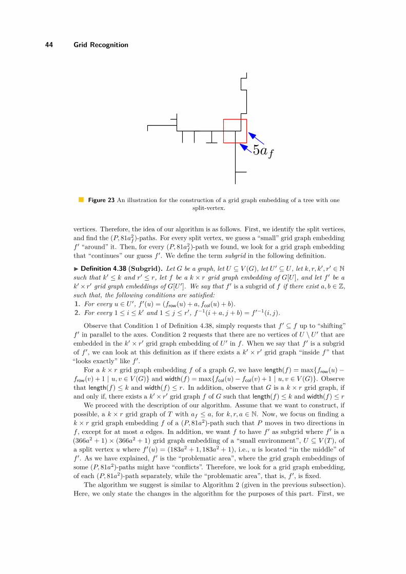
44 Grid Recognition
5af
Figure 23 An illustration for the construction of a grid graph embedding of a tree with onesplit-vertex.
vertices. Therefore, the idea of our algorithm is as follows. First, we identify the split vertices,and find the (P, 81a2
f )-paths. For every split vertex, we guess a “small” grid graph embeddingf ′ “around” it. Then, for every (P, 81a2
f )-path we found, we look for a grid graph embeddingthat “continues” our guess f ′. We define the term subgrid in the following definition.
I Definition 4.38 (Subgrid). Let G be a graph, let U ⊆ V (G), let U ′ ⊆ U , let k, r, k′, r′ ∈ Nsuch that k′ ≤ k and r′ ≤ r, let f be a k × r grid graph embedding of G[U ], and let f ′ be ak′× r′ grid graph embeddings of G[U ′]. We say that f ′ is a subgrid of f if there exist a, b ∈ Z,such that, the following conditions are satisfied:1. For every u ∈ U ′, f ′(u) = (frow(u) + a, fcol(u) + b).2. For every 1 ≤ i ≤ k′ and 1 ≤ j ≤ r′, f−1(i+ a, j + b) = f ′−1(i, j).
Observe that Condition 1 of Definition 4.38, simply requests that f ′ ⊆ f up to “shifting”f ′ in parallel to the axes. Condition 2 requests that there are no vertices of U \ U ′ that areembedded in the k′ × r′ grid graph embedding of U ′ in f . When we say that f ′ is a subgridof f ′, we can look at this definition as if there exists a k′ × r′ grid graph “inside f” that“looks exactly” like f ′.
For a k × r grid graph embedding f of a graph G, we have length(f) = max{frow(u)−frow(v) + 1 | u, v ∈ V (G)} and width(f) = max{fcol(u)− fcol(v) + 1 | u, v ∈ V (G)}. Observethat length(f) ≤ k and width(f) ≤ r. In addition, observe that G is a k × r grid graph, ifand only if, there exists a k′× r′ grid graph f of G such that length(f) ≤ k and width(f) ≤ r
We proceed with the description of our algorithm. Assume that we want to construct, ifpossible, a k × r grid graph of T with af ≤ a, for k, r, a ∈ N. Now, we focus on finding ak × r grid graph embedding f of a (P, 81a2)-path such that P moves in two directions inf , except for at most a edges. In addition, we want f to have f ′ as subgrid where f ′ is a(366a2 + 1) × (366a2 + 1) grid graph embedding of a “small environment”, U ⊆ V (T ), ofa split vertex u where f ′(u) = (183a2 + 1, 183a2 + 1), i.e., u is located “in the middle” off ′. As we have explained, f ′ is the “problematic area”, where the grid graph embeddings ofsome (P, 81a2)-paths might have “conflicts”. Therefore, we look for a grid graph embedding,of each (P, 81a2)-path separately, while the “problematic area”, that is, f ′, is fixed.
The algorithm we suggest is similar to Algorithm 2 (given in the previous subsection).Here, we only state the changes in the algorithm for the purposes of this part. First, we
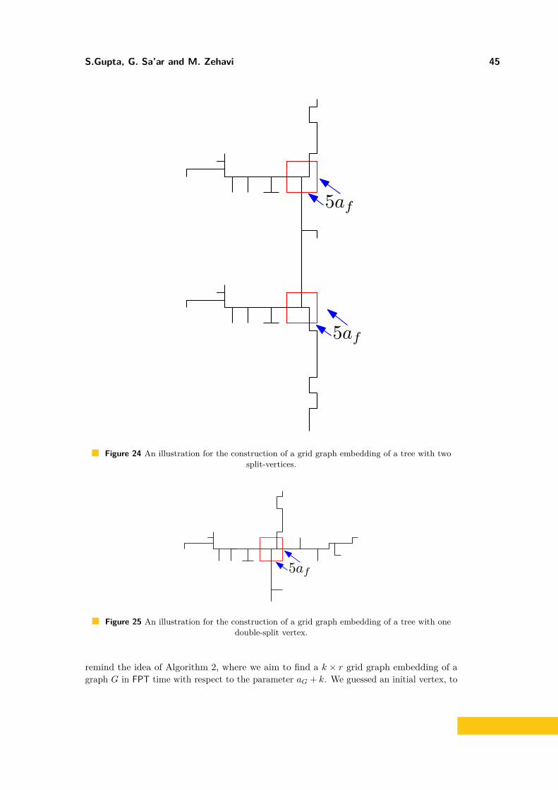
S.Gupta, G. Sa’ar and M. Zehavi 45
5af
5af
Figure 24 An illustration for the construction of a grid graph embedding of a tree with twosplit-vertices.
5af
Figure 25 An illustration for the construction of a grid graph embedding of a tree with onedouble-split vertex.
remind the idea of Algorithm 2, where we aim to find a k × r grid graph embedding of agraph G in FPT time with respect to the parameter aG + k. We guessed an initial vertex, to
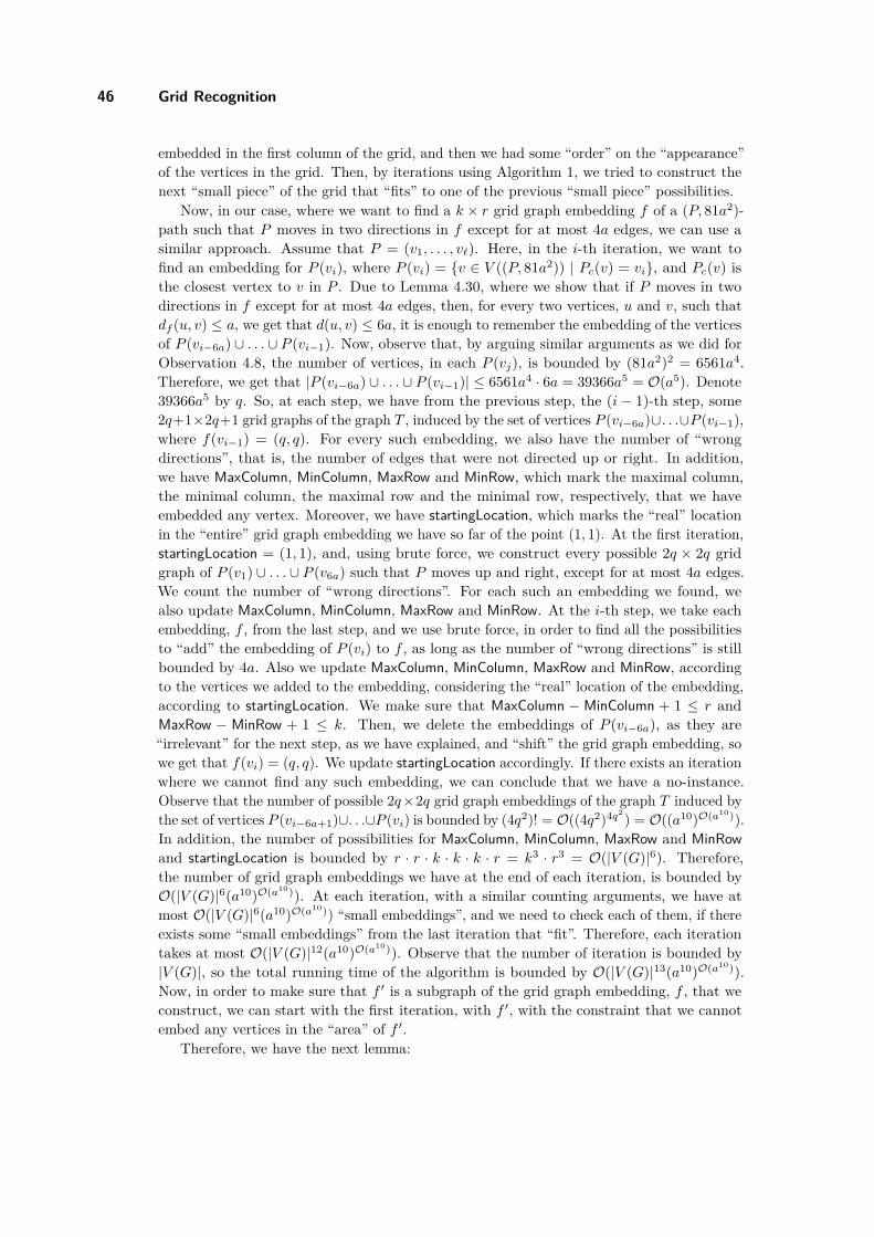
46 Grid Recognition
embedded in the first column of the grid, and then we had some “order” on the “appearance”of the vertices in the grid. Then, by iterations using Algorithm 1, we tried to construct thenext “small piece” of the grid that “fits” to one of the previous “small piece” possibilities.
Now, in our case, where we want to find a k × r grid graph embedding f of a (P, 81a2)-path such that P moves in two directions in f except for at most 4a edges, we can use asimilar approach. Assume that P = (v1, . . . , v`). Here, in the i-th iteration, we want tofind an embedding for P (vi), where P (vi) = {v ∈ V ((P, 81a2)) | Pc(v) = vi}, and Pc(v) isthe closest vertex to v in P . Due to Lemma 4.30, where we show that if P moves in twodirections in f except for at most 4a edges, then, for every two vertices, u and v, such thatdf (u, v) ≤ a, we get that d(u, v) ≤ 6a, it is enough to remember the embedding of the verticesof P (vi−6a) ∪ . . . ∪ P (vi−1). Now, observe that, by arguing similar arguments as we did forObservation 4.8, the number of vertices, in each P (vj), is bounded by (81a2)2 = 6561a4.Therefore, we get that |P (vi−6a) ∪ . . . ∪ P (vi−1)| ≤ 6561a4 · 6a = 39366a5 = O(a5). Denote39366a5 by q. So, at each step, we have from the previous step, the (i− 1)-th step, some2q+1×2q+1 grid graphs of the graph T , induced by the set of vertices P (vi−6a)∪. . .∪P (vi−1),where f(vi−1) = (q, q). For every such embedding, we also have the number of “wrongdirections”, that is, the number of edges that were not directed up or right. In addition,we have MaxColumn, MinColumn, MaxRow and MinRow, which mark the maximal column,the minimal column, the maximal row and the minimal row, respectively, that we haveembedded any vertex. Moreover, we have startingLocation, which marks the “real” locationin the “entire” grid graph embedding we have so far of the point (1, 1). At the first iteration,startingLocation = (1, 1), and, using brute force, we construct every possible 2q × 2q gridgraph of P (v1) ∪ . . . ∪ P (v6a) such that P moves up and right, except for at most 4a edges.We count the number of “wrong directions”. For each such an embedding we found, wealso update MaxColumn, MinColumn, MaxRow and MinRow. At the i-th step, we take eachembedding, f , from the last step, and we use brute force, in order to find all the possibilitiesto “add” the embedding of P (vi) to f , as long as the number of “wrong directions” is stillbounded by 4a. Also we update MaxColumn, MinColumn, MaxRow and MinRow, accordingto the vertices we added to the embedding, considering the “real” location of the embedding,according to startingLocation. We make sure that MaxColumn − MinColumn + 1 ≤ r andMaxRow − MinRow + 1 ≤ k. Then, we delete the embeddings of P (vi−6a), as they are“irrelevant” for the next step, as we have explained, and “shift” the grid graph embedding, sowe get that f(vi) = (q, q). We update startingLocation accordingly. If there exists an iterationwhere we cannot find any such embedding, we can conclude that we have a no-instance.Observe that the number of possible 2q×2q grid graph embeddings of the graph T induced bythe set of vertices P (vi−6a+1)∪. . .∪P (vi) is bounded by (4q2)! = O((4q2)4q2) = O((a10)O(a10)).In addition, the number of possibilities for MaxColumn, MinColumn, MaxRow and MinRowand startingLocation is bounded by r · r · k · k · k · r = k3 · r3 = O(|V (G)|6). Therefore,the number of grid graph embeddings we have at the end of each iteration, is bounded byO(|V (G)|6(a10)O(a10)). At each iteration, with a similar counting arguments, we have atmost O(|V (G)|6(a10)O(a10)) “small embeddings”, and we need to check each of them, if thereexists some “small embeddings” from the last iteration that “fit”. Therefore, each iterationtakes at most O(|V (G)|12(a10)O(a10)). Observe that the number of iteration is bounded by|V (G)|, so the total running time of the algorithm is bounded by O(|V (G)|13(a10)O(a10)).Now, in order to make sure that f ′ is a subgraph of the grid graph embedding, f , that weconstruct, we can start with the first iteration, with f ′, with the constraint that we cannotembed any vertices in the “area” of f ′.
Therefore, we have the next lemma:
S.Gupta, G. Sa’ar and M. Zehavi 47
I Lemma 4.39. There exists an algorithm that gets as input, a tree T , a, k, r ∈ N, a(P, t)-path in T , U ⊆ V (T ), a (366a2 + 1) × (366a2 + 1) grid graph f ′ of U and at mosttwo directions ∆ ⊂ dir, at most one horizontal direction, and at most one vertical direction.The algorithm returns “yes” if and only if there exists a k × r grid graph embedding f ′ ofT [V (P, t) ∪ U ] such that P moves in ∆ directions in f ′, except for at most 4a edges, and f ′agrees with f . In addition, the algorithm works in time O(|V (G)|13(a10)O(a10)).
In Lemma 4.39, we show the existence of an algorithm, that given a (P, t)-path, and a“small grid environment” around a split vertex, finds a k′ × r′ grid graph embeddings, of the(P, t)-paths, with the given “environment” as a subgrid, if such an embedding exists, in FPTtime. Now, we show how to use such an algorithm in order to determine if there exists ak × r grid graph embedding of T .
Assume that we are given a tree T , positive integers k, r, a ∈ N, and we want to determineif there exists a k × r grid graph embedding of T , f , such that af ≤ a. In Lemma 4.36, weproved that, if such a grid graph embedding exists, then we have few cases to consider. Thas no 81a2-split vertices, or it has exactly one split vertex, that is an 81a2-one-split vertex,or it has exactly two split vertices, that are some 81a2-one-split vertices, or it has exactly onesplit vertex, that is an 81a2-double-split vertex. For the case where T has no a-split vertices,we can simply use an algorithm that corresponds to Lemma 4.39. Now, we will prove theexistence of an algorithm that solves the case, where has one 81a2-double-split vertex, inFPT time. The other cases can be solved similarly, and we will state the differences.
In this case, we get that, by removing the only split vertex, we have four connectedcomponents, each is a (P, t)-path, where t = 81a2. We show that each such (P, t)-path“moves” to a different direction in f . Then, as we explained and as we will prove, eachembedding is “almost independent”, and there might be “overlapping” only “around” thesplit vertex. Therefore, we guess a “small environment” around the split vertex, we guessthe directions that the (P, t)-path moves, and we look for grid graph embeddings of the(P, t)-paths, such that, the “small environment” is a subgrid of them. We show that thereexists a grid graph embedding of T , if and only if, we managed to find such embeddingsthat correspond to a possible guess. We start with the easy direction, that is, if there existsa grid graph embedding f of T , then there exist a “small environment” around the splitvertex, a different “main direction” for every (P, t)-path, and grid graph embeddings of the(P, t)-paths, such that the “small environment” is a subgrid of them. We simply can take a“small environment” around the split vertex in f , and consider the “parts” of f where wehave the embedding of each (P, t)-path. We also consider the dimensions of the grid graphembedding. Since every (P, t)-path “moves” to a different direction, we have two (P, t)-pathsthat move to vertical directions, and two (P, t)-paths that move to horizontal directions. In asense, as we will prove later, the (P, t)-paths that move to vertical directions, determine thenumber of rows in the embedding, and the (P, t)-paths that move to horizontal directionsdetermine the number of columns in the embedding. We prove this direction in the nextlemma below. We first present several notations:
For a given graph G, a vertex v ∈ V , and a positive integer t ∈ N, we denote byr(v, t), the set of vertices, which in a graph distance from v, less or equal to t, that is,r(v, t) = {u ∈ V | d(u, v) ≤ t}.For a given graph G, a grid graph embedding f of G, a vertex v ∈ V , and a positiveinteger t ∈ N, we denote by (f, u, t), the t× t subgrid of G, where (f, u, t)(u) = (d t2e, d
t2e).
For a given graph G, a subset of vertices U ⊆ V , and a grid graph embedding f of G[U ],we denote U by V (f).

48 Grid Recognition
For a given graph G, a subset of vertices U ⊆ V , and a grid graph embedding f of G, wedenote by f [U ], the grid graph embedding of G[U ], defined as, f [U ](u) = f(u), for everyu ∈ U .
I Lemma 4.40. Let T = (V,E) be a tree, let k, r, a ∈ N, let f be a k×r grid graph embeddingof T . Assume that af ≤ a, and that T has exactly one 81a2-split vertex u ∈ V , that is an 81a2-double-split vertex. Let U1, U2, U3 and U4 be subsets of V such that
⋃1≤i≤4 Ui = V \{u}, Ui is
a set of vertices of a connected component in T \ {u} such that |Ui| ≥ 81a2, for i ∈ [4]. Then,there exist i1, i2, i3, i4 ∈ [4], such that ij 6= i`, for 1 ≤ j < ` ≤ 4, r1, r2, r3, r4, k1, k2, k3, k4 ∈N, U ⊆ r(u, 367a2 +1) such that u ∈ U , and a (366a2 +1)× (366a2 +1) grid graph embeddingf ′ of T [U ] such that f ′(u) = (183a2 + 1, 183a2 + 1), and the following conditions are satisfied:1. For every 1 ≤ i ≤ 3, T [Ui] is a (P, 81a2)-path.2. There exists a k1 × r1 grid graph embedding, f1, of T [Ui1 ∪ U ], such that, for every
P = (v0, . . . , v`) such that T [Ui1 ] is a (P, 81a2)-path, and Pc(u) = v0, P moves up in f1,except for at most 4a edges, and f ′ is a subgrid of f1.
3. There exists a k2 × r2 grid graph embedding, f2, of T [Ui2 ∪ U ], such that, for everyP = (v0, . . . , v`) such that T [Ui2 ] is a (P, 81a2)-path, and Pc(u) = v0, P moves left in f2,except for at most 4a edges, and f ′ is a subgrid of f2.
4. There exists a k3 × r3 grid graph embedding, f3, of T [Ui3 ∪ U ], such that, for everyP = (v0, . . . , v`) such that T [Ui3 ] is a (P, 81a2)-path, and Pc(u) = v0, P moves down inf3, except for at most 4a edges, and f ′ is a subgrid of f3.
5. There exists a k4 × r4 grid graph embedding, f4, of T [Ui4 ∪ U ], such that, for everyP = (v0, . . . , v`) such that T [Ui4 ] is a (P, 81a2)-path, and Pc(u) = v0, P moves right inf4, except for at most 4a edges, and f ′ is a subgrid of f4.
6. k1 + k3 − length(f ′) ≤ k and r2 + r4 − width(f ′) ≤ r.
Proof. Since T has exactly one 81a2-split vertex u ∈ V , we get that T [Ui] has no split-vertices, and therefore, by Lemma 4.37, T [Ui] is a (P, 81a2)-path, for every 1 ≤ i ≤ 4. Thus,Condition 1 of the lemma is satisfied. Now, it can be proved, similarly to the proof ofLemma 4.36, that for every 1 ≤ i ≤ 4, there exists a direction di ∈ dir, such that, di 6= dj ,for every 1 ≤ i < j ≤ 4, and the following condition is satisfied. For all simple paths,P 1 = (v1
0 , . . . , v1t1), P 2 = (v2
0 , . . . , v2t2), P 3 = (v3
0 , . . . , v3t3) and P 4 = (v4
0 , . . . , v4t4), such that
T [Ui] is a (P i, 81a2)-path, and P ic (u) = vi0, we get that P i moves to direction di, except for atmost 4a edges, in f i, for every 1 ≤ i ≤ 4. Let i1, i2, i3, i4 ∈ {1, 2, 3, 4} such that di1 = {up},di2 = {left}, di3 = {down} and di4 = {right}. For the sake of simplicity, we assume, withoutloss of generality, that i1 = 1, i2 = 2, i3 = 3 and i4 = 4.
Now, let f ′ = (f, u, 366a2 + 1). Observe that f ′(u) = (183a2 + 1, 183a2 + 1), and also,for every v ∈ V (f ′), df (v, u) ≤ 81a2. Therefore, since af ≤ a, for every v ∈ V (f ′), we getthat d(v, u) ≤ 81a2 + a < 82a2. So, we have that U = V (f ′) ⊆ r(u, 82a2). Now, for every1 ≤ i ≤ 4, we set f i = f [Ui ∪ U ]. In addition, for every 1 ≤ i ≤ 4, we set ki = length(f i)and ri = width(f i). Observe that this completes the proof of Conditions 2, 3, 4 and 5 of thelemma.
Now, we show that Condition 6 is satisfied. We show that argmax{frow(v) | v ∈ V } ⊆ U3.Let P 3 = (v3
0 , . . . , v3t3) such that T [U3] is a (P 3, 81a2)-path, and P 3
c (u) = v30 . Observe that
d(u, v30) ≤ 81a2+1, so df (u, v3
0) ≤ 81a2+1, and we get that frow(v30) ≥ frow(u)−81a2−1. Since
P 3 moves down in f , there exist at most a4 edges that are not directed down. We assume thatt3 > 164a2 (otherwise, observe that |U3| = O(aO(1)) and we can use brute force). Therefore,we get that frow(v3
t3) ≥ frow(v30)+164a2−4a ≥ frow(u)−81a2−1+164a2−4a > frow(u)+81a2.
Now, let v ∈ V \U3; we assume that v ∈ U2 (the other cases are similar). Let P 2 = (v20 , . . . , v
2t2)

S.Gupta, G. Sa’ar and M. Zehavi 49
such that T [U2] is a (P 2, 81a2)-path, and P 2c (u) = v2
0 . Observe that, d(u, v20) ≤ 81a2 + 1, so
df (u, v20) ≤ 81a2 + 1, and we get that frow(v2
0) ≤ frow(u) + 81a2 + 1. Since P 2 moves left inf , then, there exist at most a edges that directed down. Therefore, for every 0 ≤ i ≤ t2,frow(v2
i ) ≤ frow(v20) + a ≤ frow(u) + 82a2. Since T [U2] is a (P 2, 81a2)-path, there exists
i such that d(v, v2i ) ≤ 81a2. Therefore, df (v, v2
i ) ≤ 81a2, so frow(v) ≤ frow(v2i ) + 81a2 ≤
frow(u) + 82a2 + 81a2 = frow(u) + 163a2 < 164a2 < frow(v3t3). Thus, we proved that
argmax{frow(v) | v ∈ V } ⊆ U3. Similarly, it can be proved that argmin{frow(v) | v ∈ V } ⊆ U1,argmax{fcol(v) | v ∈ V } ⊆ U4 and argmin{frow(v) | v ∈ V } ⊆ U2.
Now, we show that argmin{f3row(v) | v ∈ V (f3)} ⊆ U . Notice that V (f3) = U ∪ U3,
and since f3 = f [U ∪ U3], it is enough to prove that argmin{frow(v) | v ∈ U ∪ U3} ⊆ U .Let P 3 = (v3
0 , . . . , v3t3) such that T [U3] is a (P 3, 81a2)-path, and P 3
c (u) = v30 . Observe that
d(u, v30) ≤ 81a2 + 1, so df (u, v3
0) ≤ 81a2 + 1, and we get that frow(v30) ≥ frow(u)− 81a2 − 1.
Since P 3 moves down in f , there are at most a edges in P 3 that are directed up. Therefore, forevery 0 ≤ i ≤ t3, frow(v3
i ) ≥ fr(v30)−a ≥ frow(u)−81a2−1−a > frow(u)−82a2. Let v ∈ U3.
Since T [U3] is a (P 3, 81a2)-path, there exists i such that d(v, v3i ) ≤ 81a2. So, df (v, v3
i ) ≤ 81a2,and we get that frow(v) ≥ frow(v3
i )− 81a2 > frow(u)− 82a2 − 81a2 = frow(u)− 163a2. Now,we show that there exists u1 ∈ U1 such that frow(u1 < frow(u)−163a2), and d(u1, u) < 325a2.Let P 1 = (v1
0 , . . . , v1t1) such that T [U1] is a (P 1, 81a2)-path, and P 1
c (u) = v10 . Observe that
d(u, v10) ≤ 81a2 + 1, so df (u, v1
0) ≤ 81a2 + 1, and we get that frow(v10) ≤ frow(u) + 81a2 − 1.
Since P 1 moves up in f , except for at most a edges, frow(v1244a2) ≤ frow(v1
0)−(244a2−a)+a ≤frow(u)+81a2−1−(244a2−a)+a = frow(u)−163a2−2a−1 < frow(u)−163a2 < frow(u3). Wegot that for u1 = v1
0 , frow(u1) < frow(u)− 163a2, and d(u1, u) < 325a2. Moreover, d(u1, u) <325a2 implies that df (u1, u) < 325a2, so u1 ∈ U . Thus, we proved that argmin{f3
row(v) | v ∈V (f3)} ⊆ U . Similarly, it can be proved that argmax{f1
row(v) | v ∈ V (f1)} ⊆ U andargmin{f1
col(v) | v ∈ V (f1)} ⊆ U and argmin{f4col(v) | v ∈ V (f4)} ⊆ U .
Now, let v3Rmax ∈ argmax{f3
row(v) | v ∈ V (f3)}, so, from what we have proved, v3Rmax ∈
argmax{frow(v) | v ∈ V }. Similarly, let v1Rmin ∈ argmin{f1
row(v) | v ∈ V (f1)}, so, from whatwe have proved, v1
Rmin ∈ argmin{frow(v) | v ∈ V }. Therefore, observe that, length(f) =frow(v3
Rmax) − frow(v1Rmin) + 1. Now, let v3
Rmin ∈ argmin{f3row(v) | v ∈ V (f3)}, so, from what
we have proved, v3Rmin ∈ argmin{f ′row(v) | v ∈ U}. Similarly, let v1
Rmax ∈ argmax{f1row(v) | v ∈
V (f1)}, so, from what we have proved, v1Rmax ∈ argmax{f ′row(v) | v ∈ U}. Therefore, we get
that length(f ′) = frow(v1Rmax) − frow(v3
Rmin) + 1, length(f1) = frow(v1Rmax) − frow(v1
Rmin) + 1,and length(f3) = frow(v3
Rmax)− frow(v3Rmin) + 1. Thus, we got that length(f) = frow(v3
Rmax)−frow(v1
Rmin) + 1 = frow(v3Rmax) − frow(v1
Rmin) + 1 + frow(v3Rmin) − frow(v3
Rmin) + frow(v1Rmax) −
frow(v1Rmax)+1−1 = frow(v3
Rmax)−frow(v3Rmin)+1+frow(v1
Rmax)−frow(v1Rmin)+1−(frow(v3
Rmax)−frow(v1
Rmin) + 1) = length(f3) + length(f1)− length(f ′) = k3 + k1 − length(f ′). In conclusion,we got that length(f) = k3 +k1− length(f ′), and therefore, k1 +k3− length(f ′) ≤ k. Similarly,it can be proved, that r2 + r4 − width(f ′) ≤ r, so Condition 6 is satisfied. J
Now, we turn to prove the opposite direction of Lemma 4.40. We are given four gridgraphs embeddings f1, f2, f3 and f4, of T [U1], T [U2], T [U3] and T [U4], correspondingly,such that each T [Ui] is a (P, 81a2)-path that “moves” to a different direction in f i, for i ∈ [4].In addition, we have “small environment”, around the split vertex u, which is a grid graphembedding f ′ of T [U ], for a subset u ∈ U ⊆ V , such that, f ′ is subgrid of f i. We show,that there exists a grid graph embedding of T . For this, we “glue” f1,f2,f3 and f4 togetheron the subgrid f ′ to get a grid graph embedding f of T . Since each f i “moves” to anotherdirection, we will prove that there is no “overlap” in f , that is, there are no two vertices thatare embedded to the same point, and therefore f is a grid graph embedding.
First, we want to define a relation between two grid graph embeddings, f1 and f2, such

50 Grid Recognition
that it is possible that V (f1) ∩ V (f2) 6= ∅. We say, that f2 agrees with f1, if we can “stick”f2 on f1, and get no “overlaps”. We define this term in the next definition:
I Definition 4.41. Let G be a graph, let U1, U2 ⊆ V (G), and let f1, f2 be grid graphembeddings of T [U1] and T [U2], correspondingly. Then, f2 agrees with f1 if there exista, b ∈ Z such that the following conditions are satisfied:1. For every u ∈ U1 ∩ U2, f1(u) = (f2
row(u) + a, f2col(u) + b).
2. For every u1 ∈ U1 \ U2, (f2)−1(f1row(u1)− a, f1
col(u1)− b) = ∅.3. For every u2 ∈ U2 \ U1, (f1)−1(f2
row(u1) + a, f1col(u1) + b) = ∅.
Assume that we have f1 and f2, that are grid graph embeddings of T [U1] and T [U2],correspondingly, such that f2 agrees with f1, and U1 ∩ U2 6= ∅. Then, observe that theintegers a, b ∈ Z that satisfy the conditions of Definition 4.41 are unique. Notice that thismeans that there is only one way to “glue” f2 with f1 such that the vertices of U1 do not“overlap” any vertex of U2, and vice versa.
Now, assume that we have U1, U2, U3, U4, U ⊆ V (G), such that, |U | ≥ 1, (Ui ∪ U) ∩(Uj ∪ U) = U , for every 1 ≤ i < j ≤ 4, and f1, f2, f3 and f4, grid graph embeddings, ofT [U1 ∪ U ], T [U2 ∪ U ], T [U3 ∪ U ] and T [U4 ∪ U ], correspondingly. Moreover, assume that, forevery {u, v} ∈ E(G), there exists i ∈ {1, 2, 3, 4}, such that, u, v ∈ Ui∪U . In addition, assumethat f j agrees with f i, for every 1 ≤ i < j ≤ 4. Then, since there is only one way to “stick”f j on f i, if we “stick” them all together, we get that none of the grid graph embeddings“overlaps” another. Therefore, this is define a “natural” way to define a grid graph embeddingof T [U1 ∪ U2 ∪ U3 ∪ U4 ∪ U ], as we define in the next observation.
I Observation 4.9. Let G be a graph, U1, U2, U3, U4, U ⊆ V (G), such that, |U | ≥ 1, V (G) =U ∪U1 ∪U2 ∪U3 ∪U4, (Ui ∪U)∩ (Uj ∪U) = U , for every 1 ≤ i < j ≤ 4, and f1, f2, f3 andf4, grid graph embeddings, of G[U1∪U ], G[U2∪U ], G[U3∪U ] and G[U4∪U ], correspondingly.Moreover, assume that, for every {u, v} ∈ E(G), there exists i ∈ {1, 2, 3, 4}, such that,u, v ∈ Ui ∪ U . In addition, assume that f j agrees with f i, for every 1 ≤ i < j ≤ 4. Leta, b, a′, b′, a′′, b′′ ∈ Z be the unique integers, such that a, b are the guaranteed integers, fromDefinition 4.41, correspond to f1 and f2, a′, b′ are the guaranteed integers, from Definition4.41, corresponding to f1 and f3, and a′′, b′′ are the guaranteed integers, correspond tof1 and f4. Let f , denoted also by f1 ∗ f2 ∗ f3 ∗ f4, be the function f : V (G) → Z × Z,defined as follows. For every u1 ∈ U1 ∪ U , f(u1) = f1(u1), for every u2 ∈ U2, f(u2) =(f2
row(u2) + a, f2col(u2) + b), for every u3 ∈ U3, f(u3) = (f3
row(u3) + a′, f3col(u3) + b′), and for
every u4 ∈ U4, f(u4) = (f4row(u4) + a′′, f4
col(u2) + b′′). Then, f is a grid graph embedding ofG.
Now, we are ready to prove the opposite direction of Lemma 4.40. We show that f jagrees with f i, for every 1 ≤ i < j ≤ 4. Then, we evoke Observation 4.9, in order to provethat there exists a grid graph embedding of T .
I Lemma 4.42. Let T = (V,E) be a tree and let a ∈ N. Assume that T has exactlyone 81a2-split vertex u ∈ V which is an 81a2-double-split vertex. Let U1, U2, U3 and U4be subsets of V such that
⋃1≤i≤4 Ui = V \ {u}, Ui is a set of vertices of a connected
component in T \ {u}and |Ui| ≥ 81a2, for i ∈ [4]. Let U ⊆ r(u, 367a2 + 1) such thatu ∈ U , and let f ′ be a (366a2 + 1) × (366a2 + 1) grid graph embedding of T [U ] such thatf ′(u) = (183a2 + 1, 183a2 + 1). Assume that there exist i1, i2, i3, i4 ∈ [4], such that ij 6= i`for 1 ≤ j < ` ≤ 4, r1, r2, r3, r4, k1, k2, k3, k4 ∈ N and the following conditions are satisfied:1. There exists a path P = (v0, . . . , v`) such that T [Ui1 ] is a (P, 81a2)-path, and Pc(u) = v0,
and a k1 × r1 grid graph embedding f1 of T [Ui1 ∪ U ] such that P moves up in f1, exceptfor at most 4a edges, and f ′ is a subgrid of f1.

S.Gupta, G. Sa’ar and M. Zehavi 51
2. There exists a path P = (v0, . . . , v`) such that T [Ui2 ] is a (P, 81a2)-path, and Pc(u) = v0,and a k2 × r2 grid graph embedding f2 of T [Ui2 ∪U ] such that P moves left in f2, exceptfor at most 4a edges, and f ′ is a subgrid of f2.
3. There exists a path P = (v0, . . . , v`) such that T [Ui3 ] is a (P, 81a2)-path, and Pc(u) = v0,and a k3 × r3 grid graph embedding f3 of T [Ui3 ∪ U ] such that P moves down in f3,except for at most 4a edges, and f ′ is a subgrid of f3.
4. There exists a path P = (v0, . . . , v`) such that T [Ui4 ] is a (P, 81a2)-path, and Pc(u) = v0,and a k4× r4 grid graph embedding f4 of T [Ui4 ∪U ] such that P moves right in f4, exceptfor at most 4a edges, and f ′ is a subgrid of f4.
5. k1 + k3 − length(f ′) ≤ k and r2 + r4 − width(f ′) ≤ r.Then, T is a k × r grid graph.
Proof. First, we show that f j agrees with f i, for every 1 ≤ i < j ≤ 4. We prove thatf3 agrees with f1, the other cases can be proved similarly. Since f ′ is subgrid of f1 andf3,V (f1) ∩ V (f3) = V (f ′), and |V (f ′)| ≥ 1, it is enough to show that for every u1 ∈ U1 \ U ,f1
row(u1) ≤ f1row(u) − 202a2, and for every u3 ∈ U3 \ U , f3
row(u3) ≥ f3row(u) − 163a2. Let
u1 ∈ U1 \ U and let P = (v0, . . . , v`) such that T [Ui1 ] is a (P, 81a2)-path, and Pc(u) = v0.Observe that f1
row(v0) ≤ f1row(u) + 81a2 + 1. Let 0 ≤ i ≤ ` be such that Pc(u1) = vi.
Observe that since u1 /∈ V (f ′), then, df1(u3, u) > 365a2, so d(u3, u) > 284a2, and sod(vi, u) ≥ 284a2, thus, i ≥ 284a2. Since P moves up in f1 except for at most a edges,f1
row(vi) ≤ f1row(v0)−284a2+a ≤ f1
row(u)−283a2. Since d(u1, vi) ≤ 81a2, so df1(u1, vi) ≤ 81a2,and we get that f1
row(u1) ≤ f1row(vi)+81a2. Therefore, we get that f1
row(u1) ≤ f1row(vi)+81a2 ≤
f1row(u)− 283a2 + 81a2 = f1
row(u)− 202a2.Now, let u3 ∈ U3 \ U and let P = (v0, . . . , v`) such that T [Ui3 ] is a (P, 81a2)-path,
and Pc(u) = v0. Observe that f3row(v0) ≥ f3
row(u) − 81a2 − 1. Since P moves down in f3,accept at most 4a edges, we get that, for every 0 ≤ i ≤ `, f3
row(vi) ≥ f3row(v0) − 4a ≥
f3row(u)− 81a2 − 1− 4a ≥ f3
row(u)− 82a2. Let 0 ≤ i ≤ `, such that, Pc(u3) = vi. Now, sinced(vi, u3) ≤ 81a2, f3
row(u3) ≥ f3row(vi)− 81a2 ≥ f3
row(u)− 82a2 − 81a2 = f3row(u)− 163a2.
We prove that f2 agrees with f1. We conclude that, f j agrees with f i, for every1 ≤ i < j ≤ 4. Therefore, we get that, the function, defined by f1∗f2∗f3∗f4, by Observation4.9, is a grid graph embedding of T . The proof that length(f1∗f2∗f3∗f4) ≤ k1+k3−length(f ′)and that width(f1 ∗ f2 ∗ f3 ∗ f4) ≤ r2 + r4 −width(f ′), is similar to the proof of Condition 6of Lemma 4.40. This ends the proof. J
Now, we present an algorithm that implements the terms we described in Lemmas 4.40and 4.42.
I Lemma 4.43. There exists an algorithm that gets as input positive integers a, k, r ∈ N,a tree T = (V,E) that has exactly one 81a2-split vertex u, which is an 81a2-double-splitvertex, the four subsets of vertices of connected components in T \ {u}, U1, U2, U3 and U4.If the algorithm returns “yes-instance”, then T is a k × r grid graph. Otherwise, there isno k × r grid graph embedding f of T such that af ≤ a. Moreover, the algorithm works inO(|V (G)|O(1)aa
O(1)).
Proof. We show that Algorithm 4 satisfies the condition of the lemma. The correctness ofthe algorithm is derived from Lemmas 4.40 and 4.42.
As for the running time, by Lemma 4.37, the computation in Line 2 takes O(|V (T )|2).Now, in Line 5, notice that the size of r(u, 367a2 + 1) is bounded by (367a2 + 1)2. The reasonfor that, is that, in a grid graph, all the vertices with graph distance, less or equal to r ∈ N,must be embedded at locations, with grid distance from u, less or equal to r, and there are
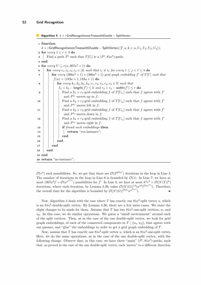
52 Grid Recognition
Algorithm 4 k × rGridRecognitiononTreeswithDouble− SplitVertex
1 functionk × rGridRecognitiononTreeswithDouble− SplitVertex(〈T, a, k, r, u, U1, U2, U3, U4〉);
2 for every 1 ≤ i ≤ 4 do3 Find a path P i such that T [Ui] is a (P i, 81a2)-path;4 end5 for every U ⊆ r(u, 367a2 + 1) do6 for every i1, i2, i3, i4 ∈ [4] such that ij 6= i` for every 1 ≤ j < ` ≤ 4 do7 for every (366a2 + 1)× (366a2 + 1)-grid graph embedding f ′ of T [U ] such that
f(u) = (183a+ 1, 183a+ 1) do8 for every k1, k2, k3, k4, r1, r2, r3, r3, r4 ∈ N such that
k1 + k3 − length(f ′) ≤ k and r2 + r4 − width(f ′) ≤ r do9 Find a k1 × r1-grid embedding f of T [Ui1 ] such that f agrees with f ′
and P i1 moves up in f ;10 Find a k2 × r2-grid embedding f of T [Ui2 ] such that f agrees with f ′
and P i2 moves left in f ;11 Find a k3 × r3-grid embedding f of T [Ui3 ] such that f agrees with f ′
and P i3 moves down in f ;12 Find a k4 × r4-grid embedding f of T [Ui4 ] such that f agrees with f ′
and P i4 moves right in f ;13 if found such embeddings then14 return “yes-instance”;15 end16 end17 end18 end19 end20 return “no-instance”;
O(r2) such possibilities. So, we get that there are O(2367a4) iterations in the loop in Line 5.The number of iterations in the loop in Line 6 is bounded by O(1). In Line 7, we have atmost (367a4)! = O(aaO(1)) possibilities for f ′. In Line 8, we have at most k4r4 = O(|V (T )|8)iterations, where each iteration, by Lemma 4.39, takes O(|V (G)|13(a10)O(a10)). Therefore,the overall time for the algorithm is bounded by O(|V (G)|O(1)aa
O(1)). J
Now, Algorithm 4 deals with the case where T has exactly one 81a2-split vertex u, whichis an 81a2-double-split vertex. By Lemma 4.36, there are a few more cases. We state theslight changes to be made for them. Assume that T has two 81a2-one-split vertices, u1 andu2. In this case, we do similar operations. We guess a “small environment” around eachof the split vertices. Then, as in the case of the one double-split vertex, we look for gridgraph embeddings, of each of the connected components in T \ {u1, u2}, that agrees withour guesses, and “glue” the embeddings in order to get a grid graph embedding of T .
Now, assume that T has exactly one 81a2-split vertex u, which is an 81a2-one-split vertex.Here, we do the same operations, as in the case of the one double-split vertex, with thefollowing change. Observe that, in this case, we have three “main” (P i, 81a2)-paths, suchthat, as proved in the case of the one double-split vertex, each ‘moves” to a different direction.
S.Gupta, G. Sa’ar and M. Zehavi 53
Therefore, since there are four directions, there might be a direction which is “not in use”.Thus, it might not be clear, as it was clear in the double-split vertex case, where are the“extreme” vertices, that is, vertices that are located in a maximum or minimum number ofrow or column. Therefore, we also need to track on the location of these extremes. In thealgorithm we described before Lemma 4.39, we also save the location of these vertices.
Observe that these changes do not change the running time of Algorithm 4 by much, andwe still have an FPT algorithms.
In Lemma 4.43, we show how to handle one of the cases from Lemma 4.36, where wewish to construct a grid graph embedding, f , of T , where af ≤ a. In addition, we state that,for every other case, there exists also an algorithm that solves that case, in a similar runningtime. Therefore, for a given a, first we need to see in what case we are, that is, how manysplit-vertices T has, and what kind of split-vertices. This clearly can be done in |V (G)O(1)|.Then, we only need an algorithm that iterates over the possibilities for a, in order to getan FPT that solves the k × r-Grid Embedding problem, with respect to aT , similarly toAlgorithm 3 of the previous subsection. We remark that we do not need to know the value ofaT in advance in order to use our algorithm, as we iterate over all the potential values of aT .
We summarize the result of this subsection in the next theorem.
I Theorem 1.6. k × r-Grid Embedding (and hence also Grid Embedding) on trees isFPT parameterized by aG.
5 Para-NP-hardness Results
In this section, we show that the k × r-Grid Embedding problem is para-NP-hard withrespect to several parameters. We start with a para-NP-hardness result with respect to theparameter k + pw.
I Theorem 1.9. k × r-Grid Embedding is NP-hard even on graphs of pathwidth 2 whenk = 3. Thus, it is para-NP-hard parameterized by k + pw, where pw is the pathwidth of theinput graph.
Proof. We give a reduction from 3-Partition. In this problem, we are given a multiset Wof 3m positive integers and the objective is to decide whether W can be partitioned into mtriplets W1,W2, . . . ,Wm such that the sum of each triplet is the same.Reduction: Given an instanceW of 3-Partition, we construct an instance G of k×r-GridEmbedding as follows. Let W = {w1, w2 . . . , w3m} be the multiset of 3m positive integersand B be the required sum for each subset of the sought partition, i.e. B =
∑W/m. Without
loss of generality, we can assume that every element inW is greater than 2 and that only sumsof exactly three elements can be equal to B, as otherwise we can get an equivalent instanceof 3-Partition with this property by adding say,
∑W to each of the elements of W and
3∑W to B. For every i ∈ [3m], we create a path Pi of size wi. Let V (Pi) = {pi1, pi2, . . . , piwi
}and E(Pi) =
⋃j∈[wi−1]
{{pij , pij+1}
}. Let P be the set of all these paths. We create m copies
of some graph G′ which, intuitively, corresponds to the sum B to be attained by each subsetof the partition, and are defined as follows (see Figure 26). For every j ∈ [m], denotethe vertex set Vj(G′) of the j-th copy of G′ by {cj1, c
j2, . . . , c
jB+4, s
j1, s
j2, . . . , s
jB+4}. Then,
we add the following edges between the vertices of Vj(G′) to get the corresponding edgeset Ej(G′): (i) for all i ∈ [B + 3], {cji , c
ji+1}, (ii) for all i ∈ [2, B + 3], {cji , s
ji}, (iii) for all
i ∈ [2, B+2], {sji , sji+1}, and (iv) {cj2, s
j1}, {c
jB+3, s
jB+4}. We finally create a graph G which is
the disjoint union ofm copies of G′ and the path P , i.e., V (G) = ∪j∈[m]Vj(G′)⋃∪i∈[3m]V (Pi)
and E(G) = ∪j∈[m]Ej(G′)⋃∪i∈[3m]E(Pi).

54 Grid Recognition
s1
c1 c2 cB+3
s2 s3
c3 cB+4
sB+4
sB+3
cB+2
sB+2
Figure 26 Example of the graph G′ built in the proof of Theorem 1.9.
We now prove that pw(G′) = 2. Consider the sequence PD = {{c1, s1, c2}, {c2, s2, c3}, {s2,
c3, s3}, . . . , {ci, si, ci+1}, {si, ci+1, si+1}, . . . , {cB+2, sB+2, cB+3}, {sB+2, cB+3, sB+3}, {cB+3,
sB+4, cB+4}}. Observe that PD is a path decomposition of G′, by Definition 2.1, pw(G′) = 2.Note that as the pathwidth of G′ is 2 and that of a path is 1, by Observation 2.1, thepathwidth of G is 2.
We now prove that W is a Yes instance of 3-Partition if and only if G is a 3× r gridgraph, where r = m(B + 4).Forward Direction: Let W be a Yes instance of 3-Partition. Let W1,W2, . . . ,Wm bea corresponding partition of W . Let Wj = {wxj
, wyj, wzj}, for every j ∈ m and some
xj , yj , zj ∈ [3m]. Let f : V (G)→ [3]× [r] be a function defined as follows (see Figure 27):(i) for all j ∈ [m], for all i ∈ [B + 4], let f(cji ) =
(2, (j − 1)(B + 4) + i
),
(ii) for all j ∈ [m], for all i ∈ [2, B + 3], let f(sji ) =(3, (j − 1)(B + 4) + i
),
(iii) for all j ∈ [m], let f(sj1) =(1, (j−1)(B+4)+2
), f(sjB+4) =
(1, (j−1)(B+4)+(B+3)
),
(iv) for all j ∈ [m], for all i ∈ [xj ], let f(pxj
i ) =(1, (j − 1)(B + 4) + 2 + i
),
(v) for all j ∈ [m], for all i ∈ [yj ], let f(pyj
i ) =(1, (j − 1)(B + 4) + 2 + wxj + i
),
(vi) for all j ∈ [m], for all i ∈ [zj ], let f(pzj
i ) =(1, (j − 1)(B + 4) + 2 + wxj
+ wyj+ i).
Note that, as for every j ∈ [m],∑Wj = B and hence wxj
+wyj+wzj
= B, it follows that fdoes not assign same value for two vertices of V (G), i.e. f is an injective function. Moreover,for every {v, u} ∈ E(G), df (u, v) = 1. So, by Definition 2.4, G is a 3× r grid graph.Reverse Direction: Let G be a 3×r grid graph. Let f be a corresponding injective function.As for every j ∈ [m],degG(cj2) = degG(cjB+3) = 4, it must be that frow(cj2) = frow(cjB+3) = 2.Also, as for every j ∈ [m] and i ∈ [2, B + 2], (cj2, c
j3, . . . , c
jB+3, s
jB+3, s
jB+2, . . . , s
j2, c
j2) and
(cji , cji+1, s
ji+1, s
ji , c
ji ) are cycles in G, it follows that for every j ∈ [m] and i ∈ [3, B + 2],
frow(cji ) = 2 and frow(sj2) = frow(sj3) = . . . = frow(sjB+3) = 1 or frow(sj2) = frow(sj3) = . . . =frow(sjB+3) = 3. Without loss of generality, assume that for every j ∈ [m] and i ∈ [2, B + 3],frow(sji ) = 3. As for every j ∈ [m], frow(cj2) = 2, frow(cj3) = 2 and frow(sj2) = 3, it must be thateither both frow(cj1) = 2 and frow(sj1) = 1 or both frow(cj1) = 1 and frow(sj1) = 2. A similarargument follows for frow(cjB+4) and frow(sjB+4). So, without loss of generality, we can alsoassume that for every j ∈ [m], frow(cj1) = frow(cjB+4) = 2 and frow(sj1) = frow(sjB+4) = 1. So,for every j ∈ [m], |fcol(cjB+4)−fcol(cj1)| = B+3. As r = m(B+4), without loss of generality, wecan assume that for every j ∈ [m] and i ∈ [B+4], fcol(cji ) = (j−1)(B+4)+i. This necessarilyimplies that for every j ∈ [m] and i ∈ [2, B + 3], fcol(sji ) = (j − 1)(B + 4) + i, fcol(sj1) =(j− 1)(B+ 4) + 2 and fcol(sjB+4) = (j− 1)(B+ 4) + (B+ 3). Therefore, as every path P ∈ Pis of size more than 2, fcol(V (P )) ∈ [fcol(cj3), fcol(cjB+2)] for some j ∈ [m]. For every j ∈ [m],let Pj be the set of paths P ∈ P with the property that fcol(V (P )) ∈ [fcol(cj3), fcol(cjB+2)]. As∑P∈P |V (P )| = mB, necessarily
∑P∈Pj
|V (P )| = B for every j ∈ [m]. By the property ofW that only three elements can sum up to B, |Pj | = 3 for every j ∈ [m]. So, for every j ∈ [m],it is well defined to denote Pj = {P j1 , P
j2 , P
j3 }. Then, we define the setWj = {|P j1 |, |P
j2 |, |P
j3 |}
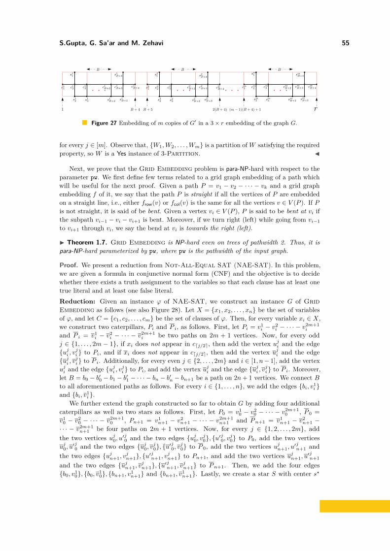
S.Gupta, G. Sa’ar and M. Zehavi 55
s21
c21 c22 c2B+3
s22 s23
c23 c2B+4
s2B+4
s2B+3
c2B+2
s2B+2
s11
c11 c12 c1B+3
s12 s13
c13 c1B+4
s1B+4
s1B+3
c1B+2
s1B+2
sm1
cm1 cm2 cmB+3
sm2 sm3
cm3 cmB+4
smB+4
smB+3
cmB+2
smB+2
B B B
1 B + 5 (m− 1)(B + 4) + 1 rB + 4 2(B + 4)
Figure 27 Embedding of m copies of G′ in a 3× r embedding of the graph G.
for every j ∈ [m]. Observe that, {W1,W2, . . . ,Wm} is a partition ofW satisfying the requiredproperty, so W is a Yes instance of 3-Partition. J
Next, we prove that the Grid Embedding problem is para-NP-hard with respect to theparameter pw. We first define few terms related to a grid graph embedding of a path whichwill be useful for the next proof. Given a path P = v1 − v2 − · · · − vk and a grid graphembedding f of it, we say that the path P is straight if all the vertices of P are embeddedon a straight line, i.e., either frow(v) or fcol(v) is the same for all the vertices v ∈ V (P ). If Pis not straight, it is said of be bent. Given a vertex vi ∈ V (P ), P is said to be bent at vi ifthe subpath vi−1 − vi − vi+1 is bent. Moreover, if we turn right (left) while going from vi−1to vi+1 through vi, we say the bend at vi is towards the right (left).
I Theorem 1.7. Grid Embedding is NP-hard even on trees of pathwidth 2. Thus, it ispara-NP-hard parameterized by pw, where pw is the pathwidth of the input graph.
Proof. We present a reduction from Not-All-Equal SAT (NAE-SAT). In this problem,we are given a formula in conjunctive normal form (CNF) and the objective is to decidewhether there exists a truth assignment to the variables so that each clause has at least onetrue literal and at least one false literal.Reduction: Given an instance ϕ of NAE-SAT, we construct an instance G of GridEmbedding as follows (see also Figure 28). Let X = {x1, x2, . . . , xn} be the set of variablesof ϕ, and let C = {c1, c2, . . . , cm} be the set of clauses of ϕ. Then, for every variable xi ∈ X,we construct two caterpillars, Pi and P i, as follows. First, let Pi = v1
i − v2i − · · · − v
2m+1i
and P i = v1i − v2
i − · · · − v2m+1i be two paths on 2m + 1 vertices. Now, for every odd
j ∈ {1, . . . , 2m − 1}, if xi does not appear in cdj/2e, then add the vertex uji and the edge{uji , v
ji } to Pi, and if xi does not appear in cdj/2e, then add the vertex uji and the edge
{uji , vji} to P i. Additionally, for every even j ∈ {2, . . . , 2m} and i ∈ [1, n− 1], add the vertex
uji and the edge {uji , vji } to Pi, and add the vertex uji and the edge {uji , v
ji} to P i. Moreover,
let B = b0 − b′0 − b1 − b′1 − · · · − bn − b′n − bn+1 be a path on 2n+ 1 vertices. We connect Bto all aforementioned paths as follows. For every i ∈ {1, . . . , n}, we add the edges {bi, v1
i }and {bi, v1
i }.We further extend the graph constructed so far to obtain G by adding four additional
caterpillars as well as two stars as follows. First, let P0 = v10 − v2
0 − · · · − v2m+10 , P 0 =
v10 − v2
0 − · · · − v2m+10 , Pn+1 = v1
n+1 − v2n+1 − · · · − v2m+1
n+1 and Pn+1 = v1n+1 − v2
n+1 −· · · − v2m+1
n+1 be four paths on 2m + 1 vertices. Now, for every j ∈ {1, 2, . . . , 2m}, addthe two vertices uj0, u′
j0 and the two edges {uj0, v
j0}, {u′
j0, v
j0} to P0, add the two vertices
uj0, u′j0 and the two edges {uj0, v
j0}, {u′
j0, v
j0} to P 0, add the two vertices ujn+1, u
′jn+1 and
the two edges {ujn+1, vjn+1}, {u′
jn+1, v
jn+1} to Pn+1, and add the two vertices ujn+1, u
′jn+1
and the two edges {ujn+1, vjn+1}, {u′
jn+1, v
jn+1} to Pn+1. Then, we add the four edges
{b0, v10}, {b0, v
10}, {bn+1, v
1n+1} and {bn+1, v
1n+1}. Lastly, we create a star S with center s?
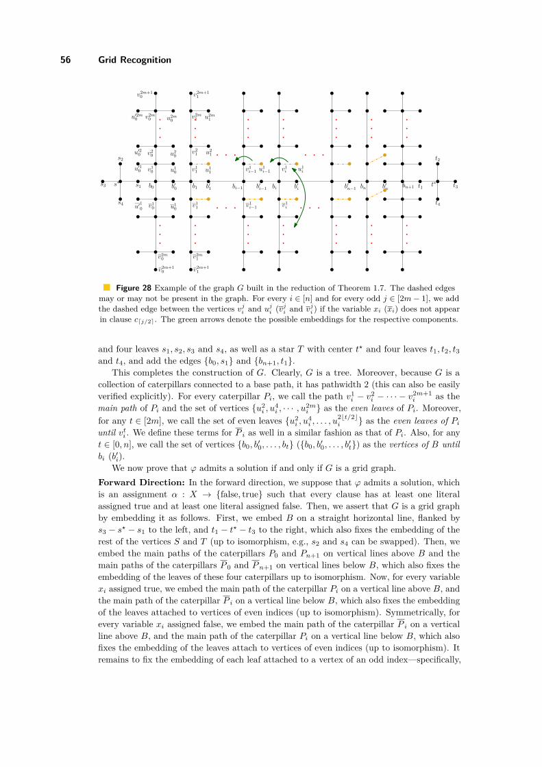
56 Grid Recognition
s3 t∗
t4
t2
t3
v2m+10 v2m+1
1
s∗
s4
s2
s1 t1bn+1b′nbnb′n−1bib′i−1 b′ibi−1b0 b′0 b1 b′1
u′10 v10 u10
u′20 v20 u20
u′2m0 v2m0 u2m0
v11
v21 u21
v2m1 u2m1
u′10
v10 u10
v11
v2m1
v2m+11
v2m0
v2m+10
v1i−1
v1i−1
v1i
v1i
u11
u1i−1 u1
i
Figure 28 Example of the graph G built in the reduction of Theorem 1.7. The dashed edgesmay or may not be present in the graph. For every i ∈ [n] and for every odd j ∈ [2m− 1], we addthe dashed edge between the vertices vji and uji (v
ji and v
ji ) if the variable xi (xi) does not appear
in clause cdj/2e. The green arrows denote the possible embeddings for the respective components.
and four leaves s1, s2, s3 and s4, as well as a star T with center t? and four leaves t1, t2, t3and t4, and add the edges {b0, s1} and {bn+1, t1}.
This completes the construction of G. Clearly, G is a tree. Moreover, because G is acollection of caterpillars connected to a base path, it has pathwidth 2 (this can also be easilyverified explicitly). For every caterpillar Pi, we call the path v1
i − v2i − · · · − v
2m+1i as the
main path of Pi and the set of vertices {u2i , u
4i , · · · , u2m
i } as the even leaves of Pi. Moreover,for any t ∈ [2m], we call the set of even leaves {u2
i , u4i , . . . , u
2bt/2ci } as the even leaves of Pi
until vti . We define these terms for P i as well in a similar fashion as that of Pi. Also, for anyt ∈ [0, n], we call the set of vertices {b0, b
′0, . . . , bt} ({b0, b
′0, . . . , b
′t}) as the vertices of B until
bi (b′i).We now prove that ϕ admits a solution if and only if G is a grid graph.
Forward Direction: In the forward direction, we suppose that ϕ admits a solution, whichis an assignment α : X → {false, true} such that every clause has at least one literalassigned true and at least one literal assigned false. Then, we assert that G is a grid graphby embedding it as follows. First, we embed B on a straight horizontal line, flanked bys3 − s? − s1 to the left, and t1 − t? − t3 to the right, which also fixes the embedding of therest of the vertices S and T (up to isomorphism, e.g., s2 and s4 can be swapped). Then, weembed the main paths of the caterpillars P0 and Pn+1 on vertical lines above B and themain paths of the caterpillars P 0 and Pn+1 on vertical lines below B, which also fixes theembedding of the leaves of these four caterpillars up to isomorphism. Now, for every variablexi assigned true, we embed the main path of the caterpillar Pi on a vertical line above B, andthe main path of the caterpillar P i on a vertical line below B, which also fixes the embeddingof the leaves attached to vertices of even indices (up to isomorphism). Symmetrically, forevery variable xi assigned false, we embed the main path of the caterpillar P i on a verticalline above B, and the main path of the caterpillar Pi on a vertical line below B, which alsofixes the embedding of the leaves attach to vertices of even indices (up to isomorphism). Itremains to fix the embedding of each leaf attached to a vertex of an odd index—specifically,
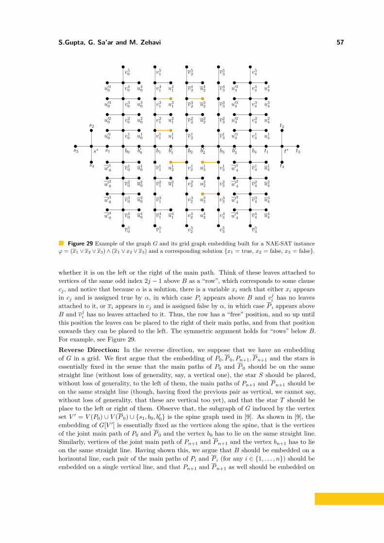
S.Gupta, G. Sa’ar and M. Zehavi 57
v41
s3
v50 v51
s∗
s4
s2
s1 b0 b′0 b1 b′1
u′10 v10 u10
u′20 v20 u20
u′40 v40 u40
v11
v21 u21
u41
u′10
v10 u10 v11
v41
v51
v40
v50
u11
b2 b′2 b3 b′3
u41
v31 u31u′30 v30 u3
0
v21
v31
u′20
v20 u20
u′30
v30 u30
u′40
u40
u21
v54
b4
u′14 v14 u14
u′24 v24 u24
u′44 v44 u44
u′14
v14 u14
v44
v54
u′34 v34 u34
u′24
v24 u24
u′34
v34 u34
u′44
u44
t∗
t4
t2
t3t1
v52
v12
v22 u22
v42 u42
u12
v32
v52
v13
v43
v53
v23
v33
v53
v13
v23
v43
u13
v33
u33
v12
v42
v22
v32
u42
u32
u22
Figure 29 Example of the graph G and its grid graph embedding built for a NAE-SAT instanceϕ = (x1 ∨ x2 ∨ x3)∧ (x1 ∨ x2 ∨ x3) and a corresponding solution {x1 = true, x2 = false, x3 = false}.
whether it is on the left or the right of the main path. Think of these leaves attached tovertices of the same odd index 2j − 1 above B as a “row”, which corresponds to some clausecj , and notice that because α is a solution, there is a variable xi such that either xi appearsin cj and is assigned true by α, in which case Pi appears above B and vji has no leavesattached to it, or xi appears in cj and is assigned false by α, in which case P i appears aboveB and vji has no leaves attached to it. Thus, the row has a “free” position, and so up untilthis position the leaves can be placed to the right of their main paths, and from that positiononwards they can be placed to the left. The symmetric argument holds for “rows” below B.For example, see Figure 29.Reverse Direction: In the reverse direction, we suppose that we have an embeddingof G in a grid. We first argue that the embedding of P0, P 0, Pn+1, Pn+1 and the stars isessentially fixed in the sense that the main paths of P0 and P 0 should be on the samestraight line (without loss of generality, say, a vertical one), the star S should be placed,without loss of generality, to the left of them, the main paths of Pn+1 and Pn+1 should beon the same straight line (though, having fixed the previous pair as vertical, we cannot say,without loss of generality, that these are vertical too yet), and that the star T should beplace to the left or right of them. Observe that, the subgraph of G induced by the vertexset V ′ = V (P0) ∪ V (P 0) ∪ {s1, b0, b
′0} is the spine graph used in [9]. As shown in [9], the
embedding of G[V ′] is essentially fixed as the vertices along the spine, that is the verticesof the joint main path of P0 and P 0 and the vertex b0 has to lie on the same straight line.Similarly, vertices of the joint main path of Pn+1 and Pn+1 and the vertex bn+1 has to lieon the same straight line. Having shown this, we argue that B should be embedded on ahorizontal line, each pair of the main paths of Pi and P i (for any i ∈ {1, . . . , n}) should beembedded on a single vertical line, and that Pn+1 and Pn+1 as well should be embedded on

58 Grid Recognition
a single vertical line, with the star T to the right of it. In particular, this argument makesuse of the even leaves of the caterpillars Pi and P i. To prove this, we first give the followingclaim.
B Claim 5.1. Let i ∈ N such that i ∈ [1, n]. Given any grid graph embedding of the graphG, if all the vertices of B until b′i−1 are embedded on a horizontal line, the main path ofPi−1 (P i−1) is embedded either on a vertical line or the first bend is towards the right (left)and the even leaves of Pi−1 (P i−1) until the first bend is towards the right (left), then thefollowing conditions are satisfied.(i) The path B is bent at neither b′i−1 nor bi.(ii) The main path of Pi (P i) is embedded either on a vertical line or the first bend is
towards the right (left).(iii) The even leaves of Pi (P i) until the first bend are towards the right (left) of the main
path of Pi (P i).
Proof. We prove the claim for Pi. The proof for P i is similar. Note that the vertices withodd superscript of the main path of Pi may or may not have a leaf attached to them. Thus,without loss of generality, for the proof of the claim we assume that there are no leavesattached to the vertices with odd superscript of the main path of Pi (which is less restrictivefor the embedding).
We first prove Condition (i). Assume first, for contradiction, that the path B is bentat b′i−1. Then, the vertex bi is placed above or below b′i−1. As degG(bi) = 4, one of itsneighbors is embedded at the same position as that of v1
i−1 or v1i−1; see Figure 30a. This is a
contradiction as in any grid graph embedding, any two distinct vertices are embedded at twodifferent positions.
Assume now, for contradiction, that the path B is bent at bi. Then, the vertex b′i isplaced above or below bi. Assume without loss of generality that b′i is placed above bi. Then,the vertex bi+1 is placed to the left or right or above of b′i. As degG(bi+1) = 4, if bi+1 isplaced to the left of b′i, then one of its neighbors is embedded at the same position at that ofb′i−1; see Figure 30b. If bi+1 is placed to the right of b′i, then one of its neighbors is embeddedat the same position as that of one of the neighbors of bi; see Figure 30c. If bi+1 is placedon the top of b′i, then one of its neighbors is embedded at the same position at that of oneof the neighbors of v2
i−1 due to the fact that either the main path of Pi−1 is bent right atv2i−1 or the leaf u2
i−1 is towards the right; see Figure 30d. In all these cases, this results in acontradiction as in any grid graph embedding, any two distinct vertices are embedded at twodifferent positions.
We now prove Condition (ii). Assume first that the main path of Pi−1 is embedded on avertical line. Towards a contradiction, suppose that the first bend of the main path of Piis at vji towards the left. If j is odd, then one of the neighbors of vj+1
i is embedded at thesame position as that of vji−1 or uj−1
i−1 or uj+1i−1 , a contradiction; see Figure 30e. If j is even,
then vj+1i is embedded at the same position as that of uji−1, a contradiction; see Figure 30f.
Thus, in this case, the main path of Pi is embedded either on a vertical line or the first bendis towards the right.
Assume now that the first bend of main path of Pi−1 is at vji−1 towards the right. Bythe above argument, we can conclude that if the first bend of Pi is at vj
′
i where j′ < j,then Pi is bent at vj
′
i towards right. Thus, we assume that if Pi is bent, the first bend isat vj
′′
i where j′′ ≥ j. We prove that if j′′ ≥ j, then j is even and j′′ = j. Assume first, bycontradiction, that j is odd. Then, one of the neighbors of vj+1
i−1 is embedded at the same
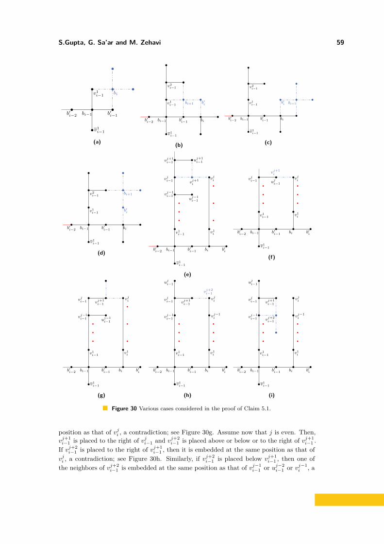
S.Gupta, G. Sa’ar and M. Zehavi 59
biv1i−1
v1i−1
bi−1 b′i−1b′i−2
(a)
v1i−1
v1i−1
bi−1 b′i−1b′i−2 bi
b′ibi+1
v2i−1
(b)
v1i−1
v1i−1
bi−1 b′i−1b′i−2 bi
b′i bi+1
v2i−1
(c)
v1i−1
v1i−1
bi−1 b′i−1b′i−2 bi
b′i
bi+1v2i−1
(d)
v1i−1
v1i−1
bi−1 b′i−1b′i−2 bi b′i
v1i
vjivj+1i
vji−1
vj+1i−1
vj−1i−1
uj+1i−1
uj−1i−1
(e)
v1i−1
v1i−1
bi−1 b′i−1b′i−2 bi b′i
vji−1vjiuj
i−1
vj+1i
v1i
(f)
v1i−1
v1i−1
bi−1 b′i−1b′i−2 bi b′i
v1i
vj−1i−1
vji−1
uj−1i−1
vj+1i−1
vji
(g)
v1i−1
v1i−1
bi−1 b′i−1b′i−2 bi b′i
v1i
vj−1i−1
vji−1 vj+1i−1
vji
vj−1i
vj+2i−1
uji−1
(h)
v1i−1
v1i−1
bi−1 b′i−1b′i−2 bi b′i
v1i
vj−1i−1
vji−1 vj+1i−1
vji
vj−1ivj+2
i−1
uji−1
(i)
Figure 30 Various cases considered in the proof of Claim 5.1.
position as that of vji , a contradiction; see Figure 30g. Assume now that j is even. Then,vj+1i−1 is placed to the right of vji−1 and vj+2
i−1 is placed above or below or to the right of vj+1i−1 .
If vj+2i−1 is placed to the right of vj+1
i−1 , then it is embedded at the same position as that ofvji , a contradiction; see Figure 30h. Similarly, if vj+2
i−1 is placed below vj+1i−1 , then one of
the neighbors of vj+2i−1 is embedded at the same position as that of vj−1
i−1 or uj−2i−1 or vj−1
i , a

60 Grid Recognition
v1i−1
v1i−1
bi−1 b′i−1b′i−2 bi b′i
v1i
vj−1i−1
vji−1 vj+1i−1
vji
vj−1i
uji−1 vj+2
i−1vj+1i
(j)
Figure 30 Various cases considered in the proof of Claim 5.1 (cont.)
contradiction; see Figure 30i. So, vj+2i−1 is placed above vj+1
i−1 . If j′′ > j, one of the neighborsof vj+2
i−1 is embedded at the same position as that of vj+1i , a contradiction; see Figure 30j.
Thus, j′′ = j.We finally prove Condition (iii). By above arguments, we know that if the first bend of
the main path of Pi−1 is at vji−1 towards the right, then the first bend of the main path ofPi−1 is at vj
′
i−1 towards the right, where j′ ≤ j. Observe that, since the even leaves of Pi−1until the first bend are towards the right, we cannot put any even leaf uki , for any k < j, ofPi towards the left as otherwise it will be embedded at the same position as that of uki−1, acontradiction. Thus, the even leaves of Pi until the first bend are towards the right. Thiscompletes the proof of the claim. J
We now return to the proof of the theorem. As we have already proved that the verticesof the joint main path of P0 and P 0 and the vertex b0 lie on the same straight line, byinductive use of the above claim, we can conclude that the path B is straight until bn and ifthe main path of Pi (P i) is bent towards the right (left), then the main path of every Pj(P j), for every j ∈ [i+ 1, n], is bent towards right (left). Observe that, as the vertices of thejoint main path of Pn+1 and Pn+1 and the vertex bn+1 lie on the same straight line, themain path of Pn cannot be bent as otherwise one of the vertex of the main path of Pn willbe embedded at the same position as that of one of the leaves of Pn+1. This implies that,each pair of the main paths of Pi and P i (for any i ∈ [n]) are embedded on a single verticalline, and that Pn+1 and Pn+1 as well are embedded on a single vertical line, with the star Tto the right of it.
Having proved this, we now define an assignment α : X → {false, true} as follows. Forevery variable xi ∈ X, if Pi is embedded above B, then we define α(xi) to be true, andotherwise we define α(xi) to be false. To argue that this assignment is a solution, considersome arbitrary clause cj . Now, consider the “row” above B that consists of the verticesv2j−1
1 , v2j−12 , . . . , v2j−1
n possibly with negations above some of them. So that the embeddingcan be valid, it must be that at least one of these vertices, say, v2k−1
i (possibly negated), hasno leaves attached to it, which means that the literal corresponding to it (which is xi or xi,

S.Gupta, G. Sa’ar and M. Zehavi 61
depending on whether v2k−1i is negated) appears in cj , and as it is assigned true by α, we
get that the clause cj is satisfied. Symmetrically, by considering the “row” below B thatconsists of the vertices v2j−1
1 , v2j−12 , . . . , v2j−1
n possibly with negations above some of them,we can conclude that at least one literal of the clause cj is assigned false. For example, seeFigure 29. J

62 Grid Recognition
References1 Parameterized complexity in graph drawing (dagstuhl seminar 21062). https://www.dagstuhl.
de/en/program/calendar/semhp/?semnr=21062.2 Akanksha Agrawal, Grzegorz Guspiel, Jayakrishnan Madathil, Saket Saurabh, and Meirav
Zehavi. Connecting the Dots (with Minimum Crossings). In Gill Barequet and Yusu Wang,editors, Symposium on Computational Geometry (SoCG 2019), volume 129 of Leibniz In-ternational Proceedings in Informatics (LIPIcs), pages 7:1–7:17, Dagstuhl, Germany, 2019.Schloss Dagstuhl–Leibniz-Zentrum fuer Informatik. URL: http://drops.dagstuhl.de/opus/volltexte/2019/10411, doi:10.4230/LIPIcs.SoCG.2019.7.
3 Eric Allender, Tanmoy Chakraborty, David A Mix Barrington, Samir Datta, and SambuddhaRoy. Grid graph reachability problems. In 21st Annual IEEE Conference on ComputationalComplexity (CCC’06), pages 15–pp. IEEE, 2006.
4 Esther M. Arkin, Michael A. Bender, Erik D. Demaine, Sándor P. Fekete, Joseph S. B. Mitchell,and Saurabh Sethia. Optimal covering tours with turn costs. SIAM J. Comput., 35(3):531–566,2005.
5 Pradeesha Ashok, Sudeshna Kolay, Syed Mohammad Meesum, and Saket Saurabh. Para-meterized complexity of strip packing and minimum volume packing. Theor. Comput. Sci.,661:56–64, 2017.
6 Michael J. Bannister, Sergio Cabello, and David Eppstein. Parameterized complexity of1-planarity. J. Graph Algorithms Appl., 22(1):23–49, 2018.
7 Moritz Beck and Sabine Storandt. Puzzling grid embeddings. In 2020 Proceedings of theTwenty-Second Workshop on Algorithm Engineering and Experiments (ALENEX), pages94–105. SIAM, 2020.
8 Arnold D Bergstra, Bert Brunekreef, and Alex Burdorf. The effect of industry-related airpollution on lung function and respiratory symptoms in school children. Environmental Health,17(1):1–9, 2018.
9 Sandeep N Bhatt and Stavros S Cosmadakis. The complexity of minimizing wire lengths invlsi layouts. Information Processing Letters, 25(4):263–267, 1987.
10 Sujoy Bhore, Robert Ganian, Fabrizio Montecchiani, and Martin Nöllenburg. Parameterizedalgorithms for book embedding problems. In Graph Drawing and Network Visualization -27th International Symposium, GD 2019, Prague, Czech Republic, September 17-20, 2019,Proceedings, pages 365–378, 2019.
11 Thomas Bläsius, Marcus Krug, Ignaz Rutter, and Dorothea Wagner. Orthogonal graphdrawing with flexibility constraints. Algorithmica, 68(4):859–885, 2014.
12 John M. Boyer and Wendy J. Myrvold. On the cutting edge: Simplified o(n) planarity byedge addition. J. Graph Algorithms Appl., 8(3):241–273, 2004. URL: https://doi.org/10.7155/jgaa.00091, doi:10.7155/jgaa.00091.
13 CDC. Social distancing. https://www.cdc.gov/coronavirus/2019-ncov/prevent-getting-sick/social-distancing.html, November 2020.
14 Hubert Y. Chan. A parameterized algorithm for upward planarity testing. In EuropeanSymposium on Algorithms (ESA 2004), volume 3221 of Lecture Notes in Computer Science,pages 157–168. Springer, 2004. URL: https://doi.org/10.1007/978-3-540-30140-0_16,doi:10.1007/978-3-540-30140-0\_16.
15 Julia Chuzhoy, David H. K. Kim, and Rachit Nimavat. Almost polynomial hardness ofnode-disjoint paths in grids. In Proceedings of the 50th Annual ACM SIGACT Symposium onTheory of Computing, STOC 2018, Los Angeles, CA, USA, June 25-29, 2018, pages 1220–1233,2018.
16 Julia Chuzhoy, David H. K. Kim, and Rachit Nimavat. Improved approximation for node-disjoint paths in grids with sources on the boundary. In 45th International Colloquiumon Automata, Languages, and Programming, ICALP 2018, July 9-13, 2018, Prague, CzechRepublic, pages 38:1–38:14, 2018.

S.Gupta, G. Sa’ar and M. Zehavi 63
17 Marek Cygan, Fedor V. Fomin, Lukasz Kowalik, Daniel Lokshtanov, Dániel Marx, Marcin Pilip-czuk, Michal Pilipczuk, and Saket Saurabh. Parameterized Algorithms. Springer, 2015. URL:http://dx.doi.org/10.1007/978-3-319-21275-3, doi:10.1007/978-3-319-21275-3.
18 Mark de Berg, Hans L. Bodlaender, Sándor Kisfaludi-Bak, Dániel Marx, and Tom C. van derZanden. A framework for eth-tight algorithms and lower bounds in geometric intersectiongraphs. In Proceedings of the 50th Annual ACM SIGACT Symposium on Theory of Computing,STOC 2018, Los Angeles, CA, USA, June 25-29, 2018, pages 574–586, 2018.
19 Hubert de Fraysseix and Patrice Ossona de Mendez. Trémaux trees and planarity. Eur.J. Comb., 33(3):279–293, 2012. URL: https://doi.org/10.1016/j.ejc.2011.09.012, doi:10.1016/j.ejc.2011.09.012.
20 Emilio Di Giacomo, Giuseppe Liotta, and Fabrizio Montecchiani. Sketched representationsand orthogonal planarity of bounded treewidth graphs. In Graph Drawing and NetworkVisualization (GD 2019), Lecture Notes in Computer Science. Springer, 2019. To appear. URL:http://arxiv.org/abs/1908.05015.
21 Walter Didimo and Giuseppe Liotta. Computing orthogonal drawings in a variable embeddingsetting. In Algorithms and Computation (ISAAC 1998), volume 1533 of Lecture Notes inComputer Science, pages 79–88. Springer, 1998.
22 Walter Didimo, Giuseppe Liotta, and Maurizio Patrignani. On the complexity of hv-rectilinearplanarity testing. In International Symposium on Graph Drawing, pages 343–354. Springer,2014.
23 Walter Didimo, Giuseppe Liotta, and Maurizio Patrignani. HV-planarity: Algorithms andcomplexity. J. Comput. Syst. Sci., 99:72–90, 2019.
24 Reinhard Diestel. Graph Theory, 4th Edition, volume 173 of Graduate texts in mathematics.Springer, 2012.
25 Rodney G. Downey and Michael R. Fellows. Fundamentals of Parameterized Complex-ity. Texts in Computer Science. Springer, 2013. URL: http://dx.doi.org/10.1007/978-1-4471-5559-1, doi:10.1007/978-1-4471-5559-1.
26 Vida Dujmovic, Michael R. Fellows, Matthew Kitching, Giuseppe Liotta, Catherine Mc-Cartin, Naomi Nishimura, Prabhakar Ragde, Frances A. Rosamond, Sue Whitesides,and David R. Wood. On the parameterized complexity of layered graph drawing. Al-gorithmica, 52(2):267–292, 2008. URL: https://doi.org/10.1007/s00453-007-9151-1,doi:10.1007/s00453-007-9151-1.
27 Fedor V Fomin, Daniel Lokshtanov, Saket Saurabh, and Meirav Zehavi. Kernelization: theoryof parameterized preprocessing. Cambridge University Press, 2019.
28 András Frank and Éva Tardos. An application of simultaneous diophantine approximationin combinatorial optimization. Combinatorica, 7(1):49–65, 1987. URL: https://doi.org/10.1007/BF02579200, doi:10.1007/BF02579200.
29 Joseph L Ganley. Computing optimal rectilinear steiner trees: A survey and experimentalevaluation. Discrete Applied Mathematics, 90(1-3):161–171, 1999.
30 Javier García-Pérez, Nerea Fernández de Larrea-Baz, Virginia Lope, Antonio J Molina, CristinaO’Callaghan-Gordo, María Henar Alonso, Marta María Rodríguez-Suárez, Benito Mirón-Pozo,Juan Alguacil, Inés Gómez-Acebo, et al. Residential proximity to industrial pollution sourcesand colorectal cancer risk: A multicase-control study (mcc-spain). Environment International,144:106055, 2020.
31 Michael R Garey and David S. Johnson. The rectilinear steiner tree problem is np-complete.SIAM Journal on Applied Mathematics, 32(4):826–834, 1977.
32 Ashim Garg and Roberto Tamassia. On the computational complexity of upward and rectilinearplanarity testing. SIAM Journal on Computing, 31(2):601–625, 2001.
33 Angelo Gregori. Unit-length embedding of binary trees on a square grid. Information ProcessingLetters, 31(4):167–173, 1989.

64 Grid Recognition
34 Martin Grohe. Computing crossing numbers in quadratic time. J. Comput. Syst. Sci.,68(2):285–302, 2004. URL: https://doi.org/10.1016/j.jcss.2003.07.008, doi:10.1016/j.jcss.2003.07.008.
35 Magnús M. Halldórsson, Christian Knauer, Andreas Spillner, and Takeshi Tokuyama. Fixed-parameter tractability for non-crossing spanning trees. In Algorithms and Data Structures(WADS 2007), volume 4619 of Lecture Notes in Computer Science, pages 410–421. Springer,2007.
36 Dan Halperin, Oren Salzman, and Micha Sharir. Handbook of discrete and computationalgeometry. In Jacob E. Goodman, Joseph O’Rourke, and Csaba D. Tóth, editors, Handbook ofDiscrete and Computational Geometry, chapter 50, pages 1311–1342. CRC Press LLC, BocaRaton, FL, 2017.
37 Cone Health. Social distancing faq: How it helps prevent covid-19 (coronavirus) and stepswe can take to protect ourselves. https://www.conehealth.com/services/primary-care/social-distancing-faq-how-it-helps-prevent-covid-19-coronavirus-/, May 2020.
38 Patrick Healy and Karol Lynch. Two fixed-parameter tractable algorithms for testingupward planarity. Int. J. Found. Comput. Sci., 17(5):1095–1114, 2006. doi:10.1142/S0129054106004285.
39 Petr Hlinený and Marek Dernár. Crossing number is hard for kernelization. In Symposiumon Computational Geometry (SoCG 2016), volume 51 of LIPIcs, pages 42:1–42:10. SchlossDagstuhl - Leibniz-Zentrum fuer Informatik, 2016.
40 Petr Hlinený and Abhisekh Sankaran. Exact crossing number parameterized by vertex cover.In Graph Drawing and Network Visualization (GD 2019), Lecture Notes in Computer Science.Springer, 2019. To appear. URL: http://arxiv.org/abs/1906.06048.
41 John E. Hopcroft and Robert Endre Tarjan. Efficient planarity testing. J. ACM, 21(4):549–568,1974. URL: https://doi.org/10.1145/321850.321852, doi:10.1145/321850.321852.
42 John E. Hopcroft and J. K. Wong. Linear time algorithm for isomorphism of planar graphs(preliminary report). In Proceedings of the 6th Annual ACM Symposium on Theory ofComputing, April 30 - May 2, 1974, Seattle, Washington, USA, pages 172–184, 1974. URL:https://doi.org/10.1145/800119.803896, doi:10.1145/800119.803896.
43 Alon Itai, Christos H Papadimitriou, and Jayme Luiz Szwarcfiter. Hamilton paths in gridgraphs. SIAM Journal on Computing, 11(4):676–686, 1982.
44 Hendrik W. Lenstra Jr. Integer programming with a fixed number of variables. Math. Oper.Res., 8(4):538–548, 1983. URL: https://doi.org/10.1287/moor.8.4.538, doi:10.1287/moor.8.4.538.
45 Ravi Kannan. Minkowski’s convex body theorem and integer programming. Math. Oper. Res.,12(3):415–440, 1987. URL: https://doi.org/10.1287/moor.12.3.415, doi:10.1287/moor.12.3.415.
46 Ken-ichi Kawarabayashi and Bruce A. Reed. Computing crossing number in linear time. InSymposium on Theory of Computing (STOC 2007), pages 382–390. ACM, 2007.
47 Fabian Klute and Martin Nöllenburg. Minimizing crossings in constrained two-sided circulargraph layouts. In Symposium on Computational Geometry (SoCG 2018), volume 99 of LIPIcs,pages 53:1–53:14. Schloss Dagstuhl - Leibniz-Zentrum fuer Informatik, 2018.
48 Giordano Da Lozzo, David Eppstein, Michael T. Goodrich, and Siddharth Gupta.Subexponential-time and FPT algorithms for embedded flat clustered planarity. In Graph-Theoretic Concepts in Computer Science - 44th International Workshop, WG 2018, Cottbus,Germany, June 27-29, 2018, Proceedings, pages 111–124, 2018. URL: https://doi.org/10.1007/978-3-030-00256-5_10, doi:10.1007/978-3-030-00256-5\_10.
49 Giordano Da Lozzo, David Eppstein, Michael T. Goodrich, and Siddharth Gupta. C-planaritytesting of embedded clustered graphs with bounded dual carving-width. In 14th InternationalSymposium on Parameterized and Exact Computation, IPEC 2019, September 11-13, 2019,Munich, Germany, pages 9:1–9:17, 2019. URL: https://doi.org/10.4230/LIPIcs.IPEC.2019.9, doi:10.4230/LIPIcs.IPEC.2019.9.
S.Gupta, G. Sa’ar and M. Zehavi 65
50 Lisa Lockerd Maragakis. Coronavirus, social and physical distancing and self-quarantine.https://www.hopkinsmedicine.org/health/conditions-and-diseases/coronavirus/coronavirus-social-distancing-and-self-quarantine, July 2020.
51 Jaroslav Nesetril and Patrice Ossona de Mendez. Sparsity - Graphs, Structures, and Algorithms,volume 28 of Algorithms and combinatorics. Springer, 2012. URL: https://doi.org/10.1007/978-3-642-27875-4, doi:10.1007/978-3-642-27875-4.
52 Md Saidur Rahman, Shin-ichi Nakano, and Takao Nishizeki. Rectangular grid drawings ofplane graphs. Computational Geometry, 10(3):203–220, 1998.
53 Md. Saidur Rahman, Takao Nishizeki, and Mahmuda Naznin. Orthogonal drawings ofplane graphs without bends. J. Graph Algorithms Appl., 7(4):335–362, 2003. URL: https://doi.org/10.7155/jgaa.00074, doi:10.7155/jgaa.00074.
54 Sadiq M Sait and Habib Youssef. VLSI physical design automation: theory and practice,volume 6. World Scientific Publishing Company, 1999.
55 Nathan R Sturtevant. Benchmarks for grid-based pathfinding. IEEE Transactions on Compu-tational Intelligence and AI in Games, 4(2):144–148, 2012.
56 Paul Turán. A note of welcome. Journal of Graph Theory, 1(1):7–9, 1977. URL: https://doi.org/10.1002/jgt.3190010105, doi:10.1002/jgt.3190010105.
57 Christopher Umans and William Lenhart. Hamiltonian cycles in solid grid graphs. InProceedings 38th Annual Symposium on Foundations of Computer Science (FOCS), pages496–505. IEEE, 1997.
58 Martin Zachariasen. A catalog of hanan grid problems. Networks: An International Journal,38(2):76–83, 2001.
Copyright © 2022 FDOKUMEN