1 23

Statistical Methods & ApplicationsJournal of the Italian Statistical Society ISSN 1618-2510 Stat Methods ApplDOI 10.1007/s10260-012-0223-2

Accounting for animal density gradientsusing independent information in distancesampling surveys

Tiago A. Marques, Stephen T. Buckland,Regina Bispo & Brett Howland

1 23

Your article is protected by copyright and

all rights are held exclusively by Springer-

Verlag Berlin Heidelberg. This e-offprint is

for personal use only and shall not be self-

archived in electronic repositories. If you

wish to self-archive your work, please use the

accepted author’s version for posting to your

own website or your institution’s repository.

You may further deposit the accepted author’s

version on a funder’s repository at a funder’s

request, provided it is not made publicly

available until 12 months after publication.

Stat Methods ApplDOI 10.1007/s10260-012-0223-2

Accounting for animal density gradients usingindependent information in distance sampling surveys

Tiago A. Marques · Stephen T. Buckland ·Regina Bispo · Brett Howland

Accepted: 25 October 2012© Springer-Verlag Berlin Heidelberg 2012

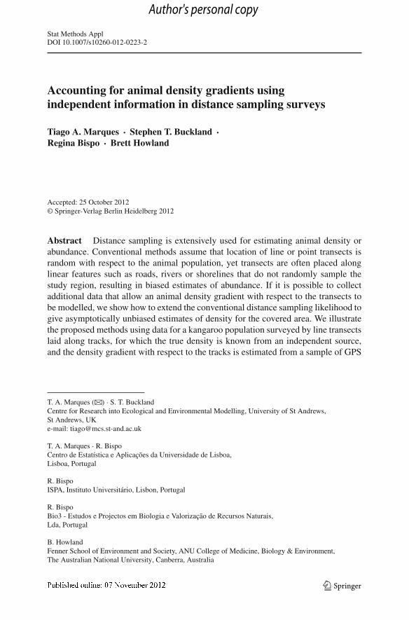
Abstract Distance sampling is extensively used for estimating animal density orabundance. Conventional methods assume that location of line or point transects israndom with respect to the animal population, yet transects are often placed alonglinear features such as roads, rivers or shorelines that do not randomly sample thestudy region, resulting in biased estimates of abundance. If it is possible to collectadditional data that allow an animal density gradient with respect to the transects tobe modelled, we show how to extend the conventional distance sampling likelihood togive asymptotically unbiased estimates of density for the covered area. We illustratethe proposed methods using data for a kangaroo population surveyed by line transectslaid along tracks, for which the true density is known from an independent source,and the density gradient with respect to the tracks is estimated from a sample of GPS

T. A. Marques (B) · S. T. BucklandCentre for Research into Ecological and Environmental Modelling, University of St Andrews,St Andrews, UKe-mail: tiago@mcs.st-and.ac.uk

T. A. Marques · R. BispoCentro de Estatística e Aplicações da Universidade de Lisboa,Lisboa, Portugal

R. BispoISPA, Instituto Universitário, Lisbon, Portugal

R. BispoBio3 - Estudos e Projectos em Biologia e Valorização de Recursos Naturais,Lda, Portugal

B. HowlandFenner School of Environment and Society, ANU College of Medicine, Biology & Environment,The Australian National University, Canberra, Australia

123

Author's personal copy

T. A. Marques et al.

collared animals. For this example, density of animals increases with distance fromthe tracks, so that detection probability is overestimated and density underestimatedif the non-random location of transects is ignored. When we account for the densitygradient, there is no evidence of bias in the abundance estimate. We end with a listof practical recommendations to investigators conducting distance sampling surveyswhere density gradients could be an issue.

Keywords Density gradients · Distance sampling · Kangaroo · Road surveys ·Line and point transects · Wildlife abundance

1 Introduction

In a world of limited resources and increasing human population, there is a growingneed to accurately and efficiently assess animal populations, to allow their effec-tive management and conservation. Therefore, methods for estimating animal abun-dance or density are increasingly required. There are a number of methods available,with mark-recapture and distance sampling being those most frequently considered(Williams et al. 2002). Unfortunately, the choice of a given method is often driven bylogistics and cost considerations rather than statistical rigour or adequacy. In particu-lar, all methods have assumptions, and their failure leads to bias. Nonetheless, theseare too frequently ignored for the sake of pragmatism. While sometimes this decisionresults from a carefully considered compromise between clearly defined objectivesand available resources, quite often this is motivated by the lack of understanding ofthe assumptions and the exact consequences of their violation.

Distance sampling is arguably the most widely used method for estimating abso-lute animal density or abundance. While the standard distance sampling reference(Buckland et al. 2001) specifies the requirement that a sufficiently large number ofsamplers, line or point transects, need to be laid at random with respect to the animaldistribution, all too often surveys are reported where landscape features are used tolay the samplers. Such landscape features might include natural structures like rivers(Fletcher and Hutto 2006), vantage points (Vargas et al. 2002), and shore lines (Georgeet al. 2004), but also man-made structures like roads (Giunchi et al. 2007; McSheaet al. 2011), fences and power lines (del Rey and Rodriguez-Lorenzo 2011). Althoughthe random location requirement might seem just a “statistician’s caprice”, it is para-mount for the derivation of the estimators involved, as we show in Sect. 2. Ignoringit can therefore potentially introduce severe bias in density estimates (e.g., Marqueset al. 2010). In fact, this bias might be as large as, or even larger than, that introducedby violations of the three other key distance sampling assumptions: (1) no animals goundetected at the line or point, (2) no animal movement, (3) no measurement error.Therefore, the consequences of the failure to use transects located at random mustbe understood. For features to which the animals respond, and hence present a non-uniform density gradient with respect to samplers laid along them, resulting densityestimates will be biased in the absence of additional information about the densitygradient. However, as we show here, if one can obtain independent information about

123

Author's personal copy

Accounting for animal density gradients

the density gradient, it can be incorporated in the estimation process by extending theconventional distance sampling likelihood.

Here we address the use of independent information about the animal density gra-dient with respect to samplers to derive asymptotically unbiased estimates of density.In Sect. 2, we describe why the random location of samplers is so important: it allowsus to assume a known distribution of animals with respect to the lines or points. Thisin turn is a corner-stone for further inference. Building on this, we show how onemight, given independent knowledge about the animal distribution with respect to thesamplers, extend the methods to deal with a spatial distribution of animals that is notindependent of the samplers. We illustrate the application of the proposed methodswith an Australian population of kangaroos in Sect. 3, sampled from road-based tran-sects. The kangaroo distribution with respect to roads along which the transects arelocated is obtained from animals fitted with GPS collars. We discuss the results inSect. 4, and present some recommendations that practitioners should consider whendealing with surveys for which density gradients with respect to samplers are likelyto occur.

2 Methods

In this section we present an overview of the key aspects of distance sampling, giv-ing the methodological basis required to develop our proposed methods. The readeris referred to Buckland et al. (2001) for further details. We consider that N animalsexist in a study area of size A, leading to animal density D = N

A . Distance samplingassumes that a sufficiently large number of samplers (lines or points) is placed atrandom in the area for which inferences are required. Usually, the entire area can-not be sampled, and hence there are two steps involved in estimating abundance forthe wider survey area: (1) using the data collected, abundance is estimated for thecovered area using model-based methods; (2) based on the estimate for the coveredarea, density is estimated for the wider region of interest usually by a design-basedapproach, which led Fewster and Buckland (2004) to refer to distance sampling asa “composite” inferential approach. Recently, the second (traditionally design-based)step has been implemented in a model-based framework (e.g., Hedley and Buckland(2004), Katsanevakis (2007)). We emphasize differences in model- and design-basedinference here because, under the presence of a density gradient, obtaining densityestimates for the wider survey area based on those from the covered area is unlikelyto be feasible under a design-based approach, as we discuss below.

For the first step, typically a systematic random sample of transects is recommended.This complicates estimation of the variance associated with encounter rate, but thatvariance is typically lower than that from simple random designs (Fewster et al. 2009).The distances yi (i = 1, 2, . . . , n) from the line or point to each of the n detected ani-mals are recorded. These distances are used to model a detection function g(y|θ),which represents the probability of detecting an animal, given that the animal is atdistance y from the line or point and θ represents the detection function parameters tobe estimated. Note that, unless otherwise required, we often drop θ in the notation forreadability. Typically, semi-parametric models are assumed for g(y), along the lines

123

Author's personal copy

T. A. Marques et al.

of Buckland (1992). These models are fitted to the sample of detected distances, andconventional model selection tools are used to choose a parsimonious model, fromwhich inference is drawn. Practitioners rarely implement model fitting themselves,relying on dedicated software to do so. The software most commonly used to analysedistance sampling data is Distance (Thomas et al. 2010). In practice, the modellingproceeds by fitting the probability density function (pdf) of detected distances, f (y),which relates directly to the detection function as:

f (y) = g(y|θ)π(y|λ)∫ w

0 g(u|θ)π(u|λ)du= g(y|θ)π(y|λ)

P(1)

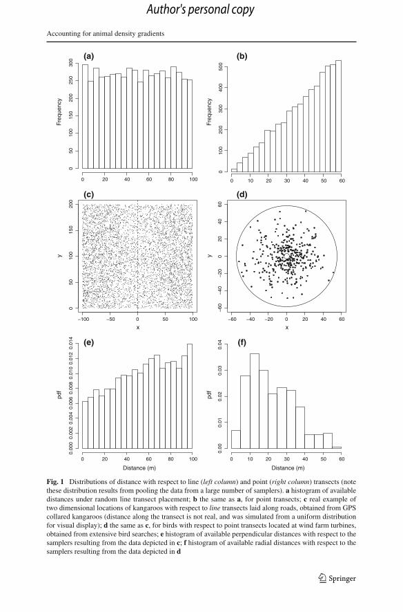
where w is a truncation distance (a distance beyond which distances are ignored), andπ(y|λ) represents the pdf of the distances available to be detected. Note that P is bydefinition the expected value of the detection function with respect to the distribu-tion of the distances available for detection; in other words, the average probabilityof detecting an animal in the covered area. Note also, in contrast with the traditionalrepresentation (e.g. Borchers and Burnham (2004), equation 3.32), the explicit useof a parameter vector λ associated with the pdf of distances available to be detected.This is fundamental for the current formulation, as we will later use non-conventionalmodels for this distribution, indexed by λ. For conventional methods, the randomlocation of samplers is fundamental. Assuming that the location of lines or pointsis random, the animal distribution within the covered areas is uniform on average,and hence π(y) = 1

w, for lines (Fig. 1a), and for points, π(y) = 2y

w2 for points (Fig.1b). Thus for conventional methods, the only unknown parameters are those from thedetection function (i.e. θ ), and hence we maximize the likelihood for θ given a sampley1 = (y1,1, y1,2, . . . , y1,n1),

L(θ |y1) =n1∏

i=1

g(y1,i |θ)π(y1,i |λ)∫ w

0 g(u|θ)π(u|λ)du(2)

allowing the estimation of θ . Following Buckland et al. (2001), the expression forconventional distance sampling density estimators is

D = n f (0)

2L= n

2Lw P(3)

in the case of line transects, where f (0) represents the estimated pdf of detecteddistances, evaluated at distance 0, and L represents the total line length and

D = nh(0)

2πk= n

kπw2 P(4)

for the case of point transects, where h(0) represents the slope of the estimated pdf ofdetected distances, evaluated at distance 0, and k represents the number of points sur-veyed. Note in both Eqs. 3 and 4 P represents an estimator of the detection probability,

123

Author's personal copy

Accounting for animal density gradients

Freq

uenc

y

0 20 40 60 80 100

050

100

150

200

250

300 (a)

Freq

uenc

y

010

020

030

040

050

0

0 10 20 30 40 50 60

(b)

−100 −50 0 50 100

050

100

150

200

x

y

(c)

−60 −40 −20 0 20 40 60

−60

−40

−20

020

4060

x

y

(d)

Distance (m)

pdf

0 20 40 60 80 100

0.00

00.

002

0.00

40.

006

0.00

80.

010

0.01

20.

014

(e)

Distance (m)

pdf

0 10 20 30 40 50 60

0.00

0.01

0.02

0.03

0.04 (f)

Fig. 1 Distributions of distance with respect to line (left column) and point (right column) transects (notethese distribution results from pooling the data from a large number of samplers). a histogram of availabledistances under random line transect placement; b the same as a, for point transects; c real example oftwo dimensional locations of kangaroos with respect to line transects laid along roads, obtained from GPScollared kangaroos (distance along the transect is not real, and was simulated from a uniform distributionfor visual display); d the same as c, for birds with respect to point transects located at wind farm turbines,obtained from extensive bird searches; e histogram of available perpendicular distances with respect to thesamplers resulting from the data depicted in c; f histogram of available radial distances with respect to thesamplers resulting from the data depicted in d

123

Author's personal copy

T. A. Marques et al.

obtained by evaluating the expression for P (cf. Eq. 1) substituting the parameters bytheir maximum likelihood estimates.

For line transect sampling, if transects are laid in such a way that the distribu-tion π(y|λ) cannot be assumed uniform, then g(y) cannot be separately estimatedin the absence of independent data, as π(y) and g(y) always appears as a product.The information about detectability and availability for detection is completely con-founded in the sighting distances, and hence g(y), and therefore P , are estimated withbias. Therefore, we need independent information about one of these two processesto proceed. By contrast, for point transect surveys in which points are not locatedrandomly, Marques et al. (2010) and Cox et al. (2011) present methods in which inde-pendent data are not required to incorporate the density gradient in the process; theseare based on assumptions for the sighting process (radial symmetry) and collection ofboth radial distances and angles. However, even here, if the density gradient extendsfurther than the truncation distance w from the points, and design-based methods areused to extrapolate beyond the covered area, then bias will occur.

Suppose that an independent sampling process, such as secondary transects perpen-dicular to the density gradient, or GPS location data in two-dimensional space (Fig.1c–f), provide a sample y2 = (y2,1, y2,2, . . . , y2,n2), drawn directly from π(y|λ).Then one can easily obtain maximum likelihood estimates for λ from the followinglikelihood

L(λ|y2) =n2∏

j=1

π(y2, j |λ). (5)

Assuming that y1 and y2 are independent (which can be enforced by proper designand survey methods), a likelihood combining the two data sources follows naturally,allowing the joint estimation of the parameters of both processes:

L(θ, λ|y1, y2) = L(θ |λ, y1)L(λ|y2) =n1∏

i=1

g(y1,i |θ)π(y1,i |λ)∫ w

0 g(u|θ)π(u|λ)du

n2∏

j=1

π(y2, j |λ). (6)

Given the parameter estimates, the usual estimate for P follows as

P =w∫

0

g(u|θ)π(u|λ)du (7)

and we can therefore obtain the corresponding estimator for density (see Eqs. 3 and4).

The above approach provides an estimate of density for the covered area. Giventhis estimate, and the estimated density gradient, one should implement a model-basedabundance estimation for the wider survey region of interest, as described in (Marqueset al. (2010), section 2.5). A purely design-based extrapolation would not be valid,as given that the density gradient exists, by definition that density is not the samenear the samplers as away from the samplers. Hence we need to model density as a

123

Author's personal copy

Accounting for animal density gradients

function of distance to the samplers, rather than inferring it by design-based consid-erations.

As for the conventional analysis methods, a straightforward way to obtain the var-iance of these density estimators might be to consider a nonparametric bootstrap.For the distance sampling survey, the recommended units for resampling are eitherthe lines or the points. For the independent source of information about the densitygradient, the appropriate sampling unit will usually be easy to identify. In the exam-ple we provide below, in which the density gradient is estimated based on a sampleof animals with GPS collars, the animals themselves would represent a reasonablesampling unit for resampling. Note that, alternatively, one could obtain variances forthe probability of detection based on the numerically differentiated Hessian matrix(which e.g. R’s optim function returns), and incorporating these with the traditionalcluster size and encounter rate variances via the delta method to obtain a densityestimate.

3 Estimating grey kangaroo abundance

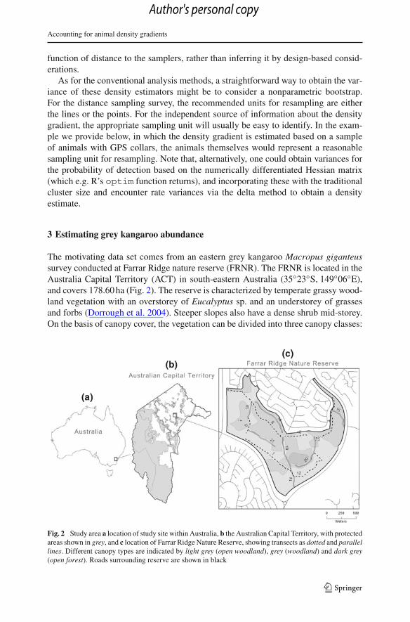
The motivating data set comes from an eastern grey kangaroo Macropus giganteussurvey conducted at Farrar Ridge nature reserve (FRNR). The FRNR is located in theAustralia Capital Territory (ACT) in south-eastern Australia (35◦23◦S, 149◦06◦E),and covers 178.60 ha (Fig. 2). The reserve is characterized by temperate grassy wood-land vegetation with an overstorey of Eucalyptus sp. and an understorey of grassesand forbs (Dorrough et al. 2004). Steeper slopes also have a dense shrub mid-storey.On the basis of canopy cover, the vegetation can be divided into three canopy classes:

Fig. 2 Study area a location of study site within Australia, b the Australian Capital Territory, with protectedareas shown in grey, and c location of Farrar Ridge Nature Reserve, showing transects as dotted and parallellines. Different canopy types are indicated by light grey (open woodland), grey (woodland) and dark grey(open forest). Roads surrounding reserve are shown in black

123

Author's personal copy

T. A. Marques et al.

open woodland, woodland and open forest. For simplicity here we ignore the effectof habitat on both detectability and availability for detection.

Distance sampling surveys of kangaroos were conducted in the 7th, 13th and 18thJuly and 5th August 2011, coinciding with a period of population stability (Fletcher2007). All transects were surveyed twice, with approximately 3.5 + 3.5 h (3.5 h ineach of 2 days) of driving required to cover the full transect length. Surveys wereundertaken 3 h after dawn, to increase the dispersion of animals, hence improvingthe efficiency of data collection. Transects were laid along existing trails. The trailnetwork was split into 15 transects based on changes in canopy type, or abrupt changein track direction (>45 degrees). Due to the closeness to the reserve boundaries, sometransects were treated as one-sided transects.

Vehicle surveys were conducted along transects, with one person driving and record-ing, while the other spotted kangaroos from an elevated position at the rear of thevehicle. Between spotting events, the vehicle was driven at speeds between 10 and15 km/h. Sighting distance and angle to kangaroos were recorded using a rangefinder(Leupold Wind River RB800). We consider the object of interest to be groups, notindividual animals: where kangaroos occurred in close proximity (within 2 m), ani-mals were recorded as a single group, with distance and angle recorded to centre ofthe group, and group size was recorded. Each encounter was recorded using a GPS(E-trex), with the actual location of kangaroos spatially mapped in ArcGIS 9.3 (ESRI2011) based on sighting coordinates and the distance and angle measurements. Per-pendicular distance was calculated from the location to the nearest point on the trackusing the NEAR command in ArcGIS. To minimize errors associated with reactivemovement, the observer scanned ahead to record animals prior to movement. Whererecorded animals moved ahead of the vehicle, the behaviour (vigilance) of newlyencountered animals was gauged to determine if animals were previously sighted, andif so, they were not included again.

A total count of the kangaroo population was conducted in 15th May 2011 using‘drive counts’ (Lancia et al. 2005; Southwell 1989). Due to population stability, itwas assumed that abundance would change negligibly between this count and the dis-tance sampling surveys. Drive counts involve observers walking across the length ofreserve within sight of each other, and counting kangaroos as they pass back throughthe line of observers. Drive counts can provide a very accurate estimate of popula-tion size when animal movement is restricted to within a relative small area, as atFRNR (Southwell 1989). Roads and housing on all sides limited kangaroo move-ment outside of the reserve, so that all animals which occur on FRNR should havebeen counted. Population size was estimated at 516 on the first drive and 517 onthe second. Given the close agreement between repeat counts no further counts wereundertaken.

To illustrate the methods, a single author (TAM) carried out all the analyses, with-out knowing the true kangaroo density. Only after the analysis was concluded was heinformed of the above estimates; taking true abundance to be 516.5 animals, densityis 2.89 animals per hectare. For illustrative purposes, to estimate mean density in thereserve, we make the simplifying assumption that average density within the trunca-tion distance w = 150 m is representative. We note that most of the reserve is within150 m of a track.

123

Author's personal copy

Accounting for animal density gradients

Conventional line transect analysis, ignoring the density gradient, was implementedin Distance 6 (Thomas et al. 2010). Numerical maximization of the required likeli-hoods for the proposed methods was implemented in R (R Development Core Team2012) using the general purpose optimization function optim.

3.1 Conventional distance sampling analysis

In total, 372 groups of kangaroos were detected. Preliminary data inspection suggestedmoderate track avoidance, and suggested that 150 m would be a reasonable truncationdistance for analysis (resulting in 351 distances). To account for possible size bias, weconsidered a size-bias regression, regressing the log of the observed cluster size on thelog of the estimated detection function. We considered three combinations to model thedetection function: (1) half-normal + cosine; (2) uniform + cosine; (3) hazard-rate +simple polynomial. It is interesting that none of the conventional goodness-of-fit testsincluding the χ2, the Cramér-von Mises and the Kolmogorov-Smirnov tests, showedevidence of a bad fit for any of these three models, with a truncation distance of either100 or 150 m. Based on minimum AIC, the hazard-rate model with no adjustment termswas selected for further inference. There was moderate evidence of size bias, with themean cluster size being 2.13 animals per group and the size-bias regression esti-mate being 1.94 animals per group. The estimated parameters of the hazard-rate wereσ = 94.9 and b = 3.1 for the scale and shape parameter, respectively. The averageprobability of detection of an animal in the covered strip was estimated to be 0.73 (95 %CI 0.67,0.81). The estimated density was 2.3 animals per hectare (95 % CI 1.60,3.31).

3.2 Modelling the distribution of animals with respect to the road

As part of a separate movement study being conducted by the Conservation Planningand Research unit of the ACT Government, location information on a sample of 23 kan-garoos spread across 15 properties in the Australian Capital Territory (ACT) and oneproperty in neighbouring New South Wales (NSW) was available from GPS collar data.Of these, two animals were actually collared at FRNR. We assume that the distributionof animals with respect to the road was constant across reserves. The implications ofthis assumption are further addressed in the discussion. GPS fixes were restricted to3 h following sunrise in order to match the timing of line transect surveys. To reducethe influence of temporal correlation in animal positions, GPS fixes were separatedby 50 min, resulting in the maximum number of three fixes per animal per day.

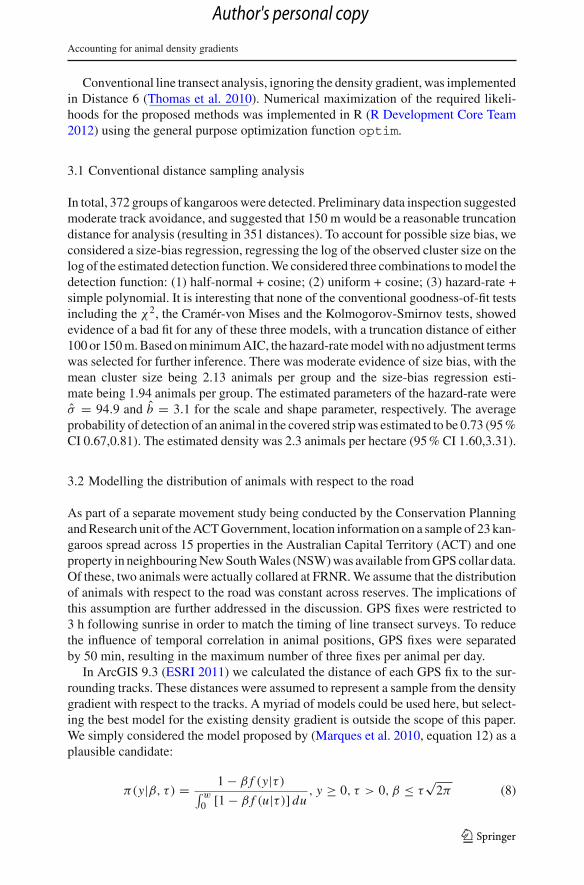
In ArcGIS 9.3 (ESRI 2011) we calculated the distance of each GPS fix to the sur-rounding tracks. These distances were assumed to represent a sample from the densitygradient with respect to the tracks. A myriad of models could be used here, but select-ing the best model for the existing density gradient is outside the scope of this paper.We simply considered the model proposed by (Marques et al. 2010, equation 12) as aplausible candidate:

π(y|β, τ) = 1 − β f (y|τ)∫ w

0 [1 − β f (u|τ)] du, y ≥ 0, τ > 0, β ≤ τ

√2π (8)

123

Author's personal copy

T. A. Marques et al.

Distance (m)

Den

sity

0 20 40 60 80 100

0.00

00.

002

0.00

40.

006

0.00

80.

010

0.01

2

Fig. 3 Observed distribution of animals with respect to the transects, overlaid with a fitted density gradientmodel

where f (y|τ) is the Gaussian density with mean 0 and standard deviation τ . Thisis a versatile model with an intuitive parameter interpretation. The shape parameterτ reflects the extent to which the road (or any other feature considered) has an impacton the animal distribution. The model accommodates both attraction to (β < 0), andavoidance of (β > 0), the linear feature, while β = 0 gives a uniform. Numericalmaximization of the likelihood resulted in parameter estimates (τ = 31.7, β = 36.2)

that provided an excellent fit to the data (Fig. 3). As can be seen, this model is far fromuniform, and hence we can expect the estimates reported in the previous section to bebiased.

3.3 Estimating kangaroo density accounting for the density gradient

We now implement the likelihood from Eq. 6 which incorporates both sets of data,the survey data analysed in Sect. 3.1, and the GPS data providing direct estimatesof the density gradient parameters introduced in Sect. 3.2. In an analogous context,Borchers et al. (2010, online appendix) showed that this is more efficient than treat-ing the parameter estimates from the previous section as known and estimating thedetection function parameters based on these. For the detection function, AIC nowfavours a half-normal model, with parameter estimate σ = 73.2 (AI C = 0) ratherthan the hazard-rate, with parameter estimates σ = 73.14 and b = 5.88 (AI C = 2).This probably reflects that, when the density gradient is ignored, the data suggest thatthe detection function has a broader shoulder, better represented by the hazard-ratemodel, than does the true detection function. The comparison between the estimateddetection functions ignoring and accounting for the density gradient is shown in Fig.4. The estimated probability of detection in the covered strip is now 0.54 (with eitherthe half-normal or hazard-rate detection function). As was anticipated, the observedlong tail was partially due to the increased availability of animals away from the line;hence, when accounting for the availability of animals, the detectability decreases andour density estimate increases.

123

Author's personal copy

Accounting for animal density gradients

Distance (m)

g(y)

0 50 100 150

00.

250.

50.

751

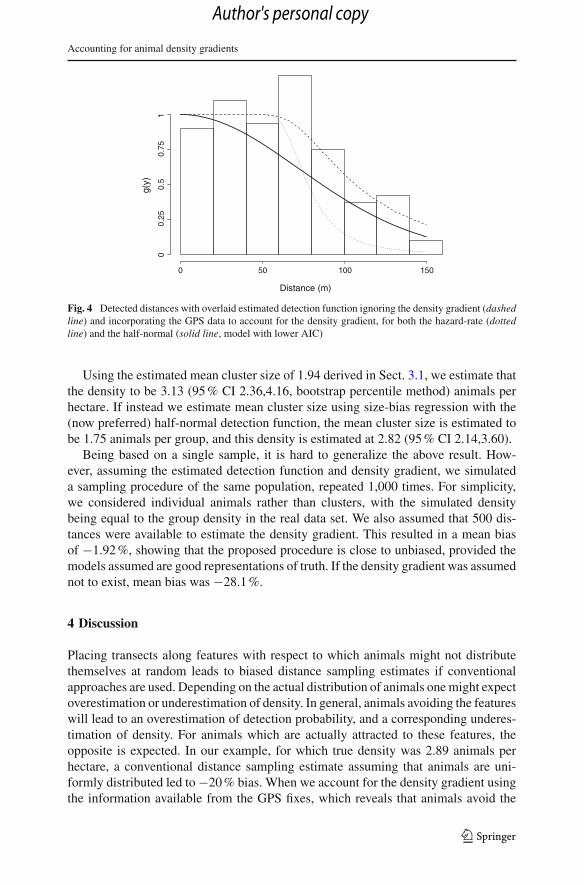
Fig. 4 Detected distances with overlaid estimated detection function ignoring the density gradient (dashedline) and incorporating the GPS data to account for the density gradient, for both the hazard-rate (dottedline) and the half-normal (solid line, model with lower AIC)

Using the estimated mean cluster size of 1.94 derived in Sect. 3.1, we estimate thatthe density to be 3.13 (95 % CI 2.36,4.16, bootstrap percentile method) animals perhectare. If instead we estimate mean cluster size using size-bias regression with the(now preferred) half-normal detection function, the mean cluster size is estimated tobe 1.75 animals per group, and this density is estimated at 2.82 (95 % CI 2.14,3.60).

Being based on a single sample, it is hard to generalize the above result. How-ever, assuming the estimated detection function and density gradient, we simulateda sampling procedure of the same population, repeated 1,000 times. For simplicity,we considered individual animals rather than clusters, with the simulated densitybeing equal to the group density in the real data set. We also assumed that 500 dis-tances were available to estimate the density gradient. This resulted in a mean biasof −1.92 %, showing that the proposed procedure is close to unbiased, provided themodels assumed are good representations of truth. If the density gradient was assumednot to exist, mean bias was −28.1 %.

4 Discussion

Placing transects along features with respect to which animals might not distributethemselves at random leads to biased distance sampling estimates if conventionalapproaches are used. Depending on the actual distribution of animals one might expectoverestimation or underestimation of density. In general, animals avoiding the featureswill lead to an overestimation of detection probability, and a corresponding underes-timation of density. For animals which are actually attracted to these features, theopposite is expected. In our example, for which true density was 2.89 animals perhectare, a conventional distance sampling estimate assuming that animals are uni-formly distributed led to −20 % bias. When we account for the density gradient usingthe information available from the GPS fixes, which reveals that animals avoid the

123

Author's personal copy

T. A. Marques et al.

vicinity of the roads along which transects were laid, the bias was reduced to 8.3 %.Note that the bias introduced in the detection function estimation also propagates intothe cluster size bias correction via the size-bias regression, because the log of theestimated detection function is used as the independent variable. The effect of the sizebias was stronger if one conducted the analysis using the detection function estimatedaccounting for the density gradient, with the estimated mean cluster size being 1.75animals per group, leading to a density estimate of 2.82 animals per hectare. Thistranslates to a further improvement in terms of percentage bias, now as low as −2.4 %.A similar value of around −2 % bias was obtained for a small simulation based on thesame parameters as observed during the survey.

When looking at the survey data (Fig. 4), one could have anticipated problemsbecause there was a slight increase in number of detections with distance from thetracks. In general, ignoring the density gradient, this could have been attributed toresponsive movement away from the observer. As we have shown here, it is actuallymore likely that this was simply the combined effect of detection and availability. Animportant point to make is that for lines, and especially if animals avoid the featureswith respect to which transects were laid, visual inspection of the data might hint atpotential problems. However, if the animals are attracted to the linear features alongwhich line transects are laid (as in e.g. Butler et al., 2005), or in the case of pointtransects, the recorded detection distances might not contain any features indicativeof the failure of the uniformity assumption. Therefore, extra care should be taken inthis case. In particular for points, as suggested by Marques et al. (2010), recording thesighting angle might allow assessment of the plausibility of the uniformity assumption,and even better, allow incorporation of non-uniform distributions. However, due to theadded complexity and inherent additional sources of variability, we only recommendaccounting for the density gradient when it cannot be avoided by proper survey design.

Two particular features arising from the case study are worth discussion. First, themodel required for the detection function becomes simpler (one parameter rather thantwo) when one accounts for the density gradient. This is intuitive: if part of the varia-tion in the data is explained by the density model, less remains to be explained by thedetection function model. Second, the bias introduced by the density gradient has animpact on the estimated detection function, and hence on the probability of detection,but it can also have an impact on the estimation of the mean group size. Again, this isobvious (at least after the fact!), because mean group size is estimated building on theestimated detection function.

For the analyses of the kangaroo data, several simplifying choices were purelypragmatic, and justified on the basis of the proof-of-concept nature of this work. How-ever, these could be improved upon if approximately unbiased density estimation wasthe key objective. The first point to raise is that strictly the corrected density estimateis valid in the vicinity of 150 m from the roads. Due to the spatial scale involved,we assume that this was a reasonable approximation to the density in the reserve.One could argue that the spatial density model should be used to calculate density inthe entire reserve, as described by Marques et al. (2010). We assumed that the den-sity gradient, estimated from the available sample of 23 kangaroos with GPS collarsfrom 16 reserves, was representative of the density gradient with respect to roads inthe sampled reserve. Additional analysis of similar GPS data as a function of spa-

123

Author's personal copy

Accounting for animal density gradients

tial location might be required to confirm, or disprove, this assumption. Further weassumed that there were no differences in detectability or availability for detectionas a function of habitat. One should try to account for habitat differences in both ofthese processes to meet biological or ecological objectives. Also, a more elegant wayof dealing with size bias would be to include group size as a covariate, along the linesof Marques and Buckland (2003) and Marques et al. (2007). Finally, model selectionand goodness-of-fit evaluation could be improved.

Testing the uniformity assumption for the species and place of interest when con-ducting distance sampling surveys should not be overlooked, especially if the transectplacement is not random. For logistical and safety reasons, roads are often preferred torandom line placement. Their effect on wildlife can be diverse. Venturato etal. (2010)showed an example in which pheasant distribution was unaffected by roads. Butleret al. (2005) showed that a wild turkey density gradient with respect to roads wasabsent in some seasons, but present in others. This suggests that care should be takenwhen quoting work from other times and places to support claims on uniformity. Quot-ing directly from Erxleben et al. (2011), “We recommend researchers and managersinvestigate animal distributions around roads before implementing road-based moni-toring programs”. Similarly, whenever lines are placed along linear features that arenot randomly located with respect to the study population, the same cautious approachshould be adopted.

Our advice for dealing with distance sampling surveys in the potential presence ofdensity gradients is simple: (1) design the survey to avoid having a density gradient ifat all possible; (2) collect data to assess to what extent a density gradient might exist.If a density gradient is expected to exist or your data point towards its existence (3),interpret results from conventional methods with extreme caution, discussing possibledirection and extent of bias and (4) consider using methods that account for the den-sity gradients, either by collecting independent information on the density gradient, aspresented here, or as presented exclusively for point transect based surveys in Marqueset al. (2010) or Cox et al. (2011).

Acknowledgments TAM and RB research is partially supported by Fundação Nacional para a Ciência eTecnologia, Portugal - FCT under the project PEst-OE/MAT/UI0006/2011. We would like to thank ACTGovernment Ecologists Dr Don Fletcher and Claire Wimpenny for providing GPS collar data, and PeterHann for volunteering his time to conduct kangaroo surveys.

References

Borchers DL, Burnham KP (2004) General formulation for distance sampling. In: Buckland ST, AndersonDR, Burnham KP, Laake JL, Borchers DL, Thomas L (eds) Advanced distance sampling. OxfordUniversity Press, Oxford, pp 307–392

Borchers DL, Marques TA, Gunnlaugsson T, Jupp PE (2010) Estimating distance sampling detection func-tions when distances are measured with errors. J Agric Biol Environ Stat 15:346–361

Buckland ST (1992) Fitting density functions with polynomials. Appl Stat 41:63–76Buckland ST, Anderson DR, Burnham KP, Laake JL, Borchers DL, Thomas L (2001) Introduction to dis-

tance sampling—estimating abundance of biological populations. Oxford University Press, OxfordButler M, Wallace M, Ballard W, DeMaso S, Applegate R (2005) From the field: the relationship of Rio

Grande wild turkey distributions to roads. Wildl Soc Bull 33(2):745–748

123

Author's personal copy

T. A. Marques et al.

Cox MJ, Borchers DL, Demer DA, Cutter GR, Brierley AS (2011) Estimating the density of antarctic krill(Euphausia superba) from multi-beam echo-sounder observations using distance sampling methods.Appl Stat 60:301–316

del Rey EG, Rodriguez-Lorenzo JA (2011) Avian mortality due to power lines in the Canary Islands withspecial reference to the steppe-land birds. J Nat Hist 45:2159–2169

Dorrough J, Yen A, Turner V, Clark SG, Crosthwaite J, Hirth JR (2004) Livestock grazing management andbiodiversity conservation in Australian temperate grassy landscapes. Aust J Agric Res 55:279–295

Erxleben D, Butler M, Ballard W, Wallace M, Peterson M, Silvy N, Kuvlesky W, Hewitt D, DeMasoS, Hardin J, Dominguez-Brazil M (2011) Wild turkey (Meleagris gallopavo) association to roads:implications for distance sampling. Eur J Wildl Res 57:57–65

ESRI (2011) ArcGIS: Release 9.3. Redlands, California: Environmental Systems Research Institute 1999–2010

Fewster RM, Buckland ST (2004) Assessment of distance sampling estimators. In: Buckland ST, Ander-son DR, Burnham KP, Laake JL, Borchers DL, Thomas L (eds) Advanced distance sampling. OxfordUniversity Press, Oxford , pp 281–306

Fewster RM, Buckland ST, Burnham KP, Borchers DL, Jupp PE, Laake JL, Thomas L (2009) Estimatingthe encounter rate variance in distance sampling. Biometrics 65:225–236

Fletcher D (2007) Pest or guest: the zoology of overabundance. Chapter Managing Eastern Grey Kanga-roos Macropus giganteus in the Australian capital territory: reducing the overabundance—of opinion.Royal Zoological Society of New South Wales, Mosman, NSW, pp 117–128

Fletcher JR, Hutto LR (2006) Estimating detection probabilities of river birds using double surveys. Auk123:695–707

George J, Zeh J, Suydam R, Clark C (2004) Abundance and population trend (1978–2001) of western Arcticbowhead whales surveyed near Barrow. Mar Mamm Sci 20:755–773

Giunchi D, Gaggini V, Baldaccini N (2007) Distance sampling as an effective method for monitoring feralpigeon (Columba livia f. domestica) urban populations. Urb Ecosyst 10:397–412

Hedley SL, Buckland ST (2004) Spatial models for line transect sampling. J Agric Biol Environ Stat9(2):181–199

Katsanevakis S (2007) Density surface modelling with line transect sampling as a tool for abundance esti-mation of marine benthic species: the Pinna nobilis example in a marine lake. Mar Biol 152:77–85

Lancia RA, Kendall WL, Pollock KH, Nichols JD (2005) Estimating the number of animals in wildlife pop-ulations. In: Techniques for wildlife investigations and management. The Wildlife Society, Bethesda,MD, pp 106–153

Marques FFC, Buckland ST (2003) Incorporating covariates into standard line transect analyses. Biometrics59:924–935

Marques TA, Thomas L, Fancy SG, Buckland ST (2007) Improving estimates of bird density using multiplecovariate distance sampling. Auk 124:1229–1243

Marques TA, Buckland ST, Borchers DL, Tosh D, McDonald RA (2010) Point transect sampling alonglinear features. Biometrics 66:1247–1255

McShea WJ, Stewart CM, Kearns L, Bates S (2011) Road bias for deer density estimates at 2 national parksin Maryland. Wildl Soc Bull 35(3):177–184

R Development Core Team (2012) R: a language and environment for statistical computing. R Foundationfor Statistical Computing, Vienna, Austria. ISBN 3-900051-07-0

Southwell C (1989) Techniques for monitoring the abundance of kangaroo and wallaby populations. In:Grigg G, Jarman P, Hume I (eds) Kangaroos, wallabies and ratkangaroos, Surrey Beatty, Sydney, pp659–693

Thomas L, Buckland ST, Rexstad EA, Laake JL, Strindberg S, Hedley SL, Bishop JR, Marques TA, Burn-ham KP (2010) Distance software: design and analysis of distance sampling surveys for estimatingpopulation size. J Appl Ecol 47:5–14

Vargas A, Jimenez I, Palomares F, Palacios MJ (2002) Distribution, status, and conservation needs of thegolden-crowned sifaka (Propithecus tattersalli). Biol Conserv 108:325–334

Venturato E, Cavallini P, Dessa-Fulgheri F (2010) Are pheasants attracted or repelled by roads? A test ofa crucial assumption for transect censuses. Eur J Wildl Res 56:233–237

Williams BK, Nichols JD, Conroy MJ (2002) Analysis and management of animal populations. AcademicPress, San Diego

123

Author's personal copy