ABSTRACT

Title of Thesis: AN INVESTIGATION ON THERMAL CHARACTERISTICS OF PREMIXED COUNTERFLOW FLAMES USING MICRO-THERMOCOUPLES

Roya Ghoddoussi, Master of Science, 2005 Thesis directed by: Professor André W. Marshall Department of Fire Protection Engineering

Hydrogen addition is known to improve the stability of highly strained

hydrocarbon premixed flames. Since the flame temperature is an important factor

associated with extinction, it is of interest to study the thermal characteristics of the

hydrogen-doped flames near extinction. Temperature profiles of highly strained lean-

premixed pure CH4 and CH4/H2 flames were measured in a counterflow configuration

at strain rates far from and close to extinction. Point temperature measurements were

made utilizing a micro-thermocouple probe. To improve the measurements, the

thermocouple support design was enhanced and corrections were made for

measurement errors where appropriate. Trends observed in experimental and

modeling temperature profiles with changes in fuel composition and strain rate, agree

favorably. However, there are some discrepancies between the measured and

predicted absolute temperatures. Factors contributing to these discrepancies and the

methods to reduce the thermocouple measurement errors are discussed.

AN INVESTIGATION ON THERMAL CHARACTERISTICS OF PREMIXED COUNTERFLOW FLAMES USING MICRO-THERMOCOUPLES

By

Roya Ghoddoussi

Thesis submitted to the Faculty of the Graduate School of the University of Maryland, College Park in partial fulfillment

of the requirements for the degree of Master of Science

2005

Advisory Committee:

Professor André W. Marshall, Chair/Advisor Professor Gregory S. Jackson Professor Arnaud Trouvé

ii

Acknowledgements

First, I would like to express my deep gratitude to my research advisor

Professor André Marshall for his continuous assistance, guidance, and support

throughout this research project. With his positive attitude and infinite patience, he

has always been there to guide and help me. I am especially thankful to Professor

Gregory Jackson, my co-advisor for his insightful comments, guidance and

encouragement. I would also like to thank the other member of my thesis committee,

Professor Arnaud Trouvé for generous dedication of his time. Special thanks to

Professor Kenneth Kiger for graciously allowing me to share his lab space and

equipment. I am very thankful to Joseph Plaia, for kindly providing the numerical

modeling data used in this work, and for responding to my numerous emails and

questions, and also to Roxanna Sai for teaching me how to work with the

experimental set-up and sharing her experiences with me. I would like to thank

members of Fire Flow Research group for their friendship, assistance, and guidance

throughout my studies and research. I would also like to thank the Chair, faculty and

staff of the Department of Fire Protection Engineering for providing a friendly

educational environment and making the experience of these past years at the

University of Maryland an enjoyable one.

My special thanks to my parents and my brother, my role models, for their

words of encouragement and their belief in me. Lastly but most importantly, my

deepest appreciation and love goes to my husband Alireza Modafe for his

encouragement, support, and assistance through all the steps of this journey. I thank

him from the bottom of my heart.

iii

Table of Contents

Acknowledgements....................................................................................................... ii Table of Contents......................................................................................................... iii List of Tables ................................................................................................................v List of Figures ............................................................................................................. vi Chapter 1: Introduction .................................................................................................1 1.1 Overview................................................................................................1 1.2 Literature Review...................................................................................3 1.3 Objectives of Study .............................................................................12 Chapter 2: Approach ....................................................................................................13 2.1 Introduction .........................................................................................13 2.2 Experimental Test Facility...................................................................13 2.2.1 Test Rig ................................................................................13 2.2.2 Traverse ................................................................................15 2.3 Diagnostics ..........................................................................................17 2.3.1 Thermocouple Support Design .............................................17 2.3.2 Thermocouple Coating..........................................................20 2.3.3 Data Acquisition System.......................................................21 2.4 Temperature Measurement Methodology............................................22 Chapter 3: Data Analysis .............................................................................................24 3.1 Introduction..........................................................................................24 3.2 Thermocouple Probe Heat Transfer.....................................................25 3.2.1 Convection ............................................................................25 3.2.2 Conduction............................................................................29 3.2.3 Radiation ..............................................................................33 3.2.4 Catalysis ................................................................................38 3.3 Non-uniform Thermocouple Heating ..................................................39 3.4 Thermocouple Positioning ...................................................................40 3.5 Probe-induced Disturbances ................................................................41 3.6 Thermal Inertia ....................................................................................42 3.7 Measurement Validation .....................................................................49 3.7.1 Model Quality Assessment ...................................................49 3.7.2 Uncertainty in Experimental Parameters ..............................50 Chapter 4: Results ........................................................................................................53 4.1 Introduction .........................................................................................53 4.2 Steady Flames ......................................................................................53 4.2.1 Effects of Strain ...................................................................53 4.2.2 Effects of Fuel ......................................................................57

iv

4.3 Oscillating Flames ...............................................................................60 Chapter 5: Conclusions ................................................................................................64 Appendix A: Illustration of National Instruments LabVIEW Program Utilized for Temperature Measurement and Traverse Control .......................................................66 Appendix B: Error Analysis for Steady-State Thermocouple Measurements .............71 Bibliography ................................................................................................................73

v

List of Tables

4.1 Measured and adiabatic CH4 flame temperature .............................................56 4.2 Flame width and temperature gradient ............................................................57

vi

List of Figures

1.1 Premixed methane/air flame structure ( 65.0=φ , κmean / κext = 0.8)..................3 1.2 Counterflow premixed flame .............................................................................4 2.1 Rig set-up.........................................................................................................14 2.2 Experimental set-up for temperature measurement ........................................16 2.3 Thermocouple support ....................................................................................17 2.4 Thermocouple wire expansion in flame...........................................................18 2.5 Thermocouple single support design ...............................................................18 2.6 Measurement of thermocouple support temperature .......................................20 2.7 Thermocouple coating microscopic images.....................................................21 3.1 Heat transfer modes in thermocouple ..............................................................25 3.2 Calculated Nusselt numbers at a 900 K near flame location (Methane flame of

φ = 0.65 and κmean / κext = 0.8) ........................................................................27 3.3 Variation of conduction cooling error with thermocouple wire length in

methane flame (φ = 0.65, α = 0.1 and κmean / κext = 0.6)..................................30 3.4 Variation of conduction heating error with thermocouple wire length in

methane flame (φ = 0.65, α = 0.1 and κmean / κext = 0.6) .................................31 3.5 Temperature difference between thermocouple and support...........................32 3.6 Calculated radiation correction using Nusselt number correlations at a 900 K

near flame location (Methane flame of φ = 0.65 and κmean / κext = 0.8) ..........35 3.7 Effect of thermocouple wire diameter on the radiation loss (Methane flame of

φ = 0.65 and κmean / κext = 0.8) .........................................................................37 3.8 Probe induced disturbances..............................................................................41 3.9 Average temperature decay for calculation of the time constant.....................43 3.10 Experimental set-up for measuring response time of the probe ......................45

vii

3.11 100 ms of uncompensated and compensated sinusoidal signal at τ = 15 ms ..........................................................................................................................47 3.12 100 ms of uncompensated and compensated sinusoidal signal at τ = 30 ms ..........................................................................................................................48 3.13 Comparison between computed profiles and Raman scattering temperature

profiles (Case C, κmean / κext = 0.5, κext = 400 s-1).............................................50 3.14 Uncertainty in experimental conditions (a) Spherical bead geometry (b) Cylindrical bead geometry .........................................................................52 4.1 Effect of strain on CH4 flames – Measurement results (φ = 0.65) (a) α = 0.00 (b) α = 0.05 (c) α = 0.10 ..............................................................54 4.2 Effect of strain on CH4 flames – Modeling results (φ = 0.65) (a) α = 0.00 (b) α = 0.05 (c) α = 0.10 .............................................................55 4.3 Effect of H2 addition on CH4 flames – Measurement results (φ = 0.65)

(a) 60% of κext (b) CH4 at 80% and CH4/H2 at 85% of κext..............................58

4.4 Effect of H2 addition on CH4 flames – Modeling results (φ = 0.65) (a) 60% of κext (b) CH4 at 80% and CH4/H2 at 85% of κext .............................59

4.5 Changes in the flame temperature as a function of strain rate for CH4 and C3 H8. Extinction occurs at tip of the knee of the profiles ..............................60 4.6 Uncompensated and compensated temperature signatures in the methane

flame brush (φ = 0.65, α = 0.0, 15.0=′ meanuu ) ............................................61 4.7 Measured and calculated (a) mean and (b) fluctuating temperature profiles for

φ = 0.65, κmean / κext = 0.9, Tin = 300 °C for ( - α = 0.10, u’/umean = 0.0), ( - α = 0.10, u’/umean = 0.03) .................................................................................62

1

Chapter 1: Introduction 1.1 Overview

Many practical combustion systems such as gas turbines, boilers, and internal

combustion (IC) engines operate with lean premixed flames to limit combustion

temperatures and associated NOx emissions. The NOx formation rate increases

exponentially with temperature. By lowering the fuel equivalence ratio, the flame

temperature is lowered, and as a result NOx emissions are reduced [1]. However,

lowering the fuel equivalence ratio also lowers the flame stability, which may lead to

local flame extinction and increase in CO emission. The flame stability depends on

the competition of heat production from exothermic chemical reactions in flame and

heat loss due to radiation and diffusion. It has been found that addition of small

amount of hydrogen can improve the stability of lean premixed flames because of the

higher flame speed and wider flammability limits of hydrogen. Addition of H2 to the

fuel increases the flame speed, leading to faster transportation of species and faster

reactions. In addition, wide flammability limits of hydrogen supports combustion of

very lean mixtures [2]. Therefore, the hydrogen-doped flame can be stabilized at

lower flame temperatures, allowing a reduction in NOx and CO emissions [3].

In most practical combustion systems the nature of the flow is turbulent.

Under many practical conditions the turbulence can be thought to wrinkle and deform

the flame front [1]. In the wrinkled flamelet regime, turbulent flames can be modeled

as a set of stretched laminar flamelets [4]. Therefore, the results obtained from

studying stretched laminar premixed flames improve the capability to characterize the

combustion processes occurring in turbulent reacting flows.

2

The flame temperature is one of the most important variables in characterizing

flames and also in determining local heat release and reaction rates in flames.

Moreover, many of the parameters such as flame speed and thickness that are used to

analyze flames are temperature dependent [1]. Therefore studying the temperature

signature of laminar stretched flames can provide valuable information for modeling

turbulent premixed flames leading to improvement in design of practical combustion

systems.

3

1.2 Literature Review

The flame generated from a premixed fuel-oxidizer system is called a

premixed flame. If the equivalence ratio for such a system is less than one, meaning

there is an excess of oxidant present in the mixture, the flame is said to be lean.

Structure of a one-dimensional premixed methane flame, normal to the flame front is

shown in Figure 1.1. The data has been obtained from an already developed 1-D

computational model [5].

The flame is considered to be divided into three zones: a preheat zone, a

reaction zone, and a post-flame zone [6]. In the preheat zone the unburned gases

approaching the flame are heated up by the diffused heat from the reaction zone.

However, due to the presence of convective flow, the increase in the temperature

profile is not linear [7]. The majority of exothermic chemical reactions occur in the

Fig. 1.1: Premixed methane/air flame structure ( 65.0=φ , κmean / κext =0.8)

4

Flat Double Flame

Fuel + Air

Fuel + Air

Fig. 1.2: Counterflow premixed flame

reaction zone, where the gas temperature has reached the ignition temperature. The

reaction zone is typically less than 1 mm wide. Thus, the gradients of temperature

and species concentration are very large. These large gradients facilitate diffusion of

heat and radical species to the preheat zone and sustain the flame [1]. In the post

flame zone some exothermic radical recombination reactions take place. However,

the radical concentration is too low to have much effect on the temperature profile.

The counterflow flame configuration is commonly used to study the behavior

of stretched flames. This flame can be produced from impinging two streams of

coaxially opposed combustible mixture (Figure 1.2). At high strain rates the twin

counterflow flames are pushed to the stagnation plane to keep the balance between

the flame speed and the flow velocity. At these conditions the classic double flame

counterflow structure merge and appear as a single flat and symmetrical flame at the

stagnation plane.

5

Counterflow flames are of fundamental research interest since at the centerline

of the nozzles gradients only exist in the axial direction and the flow can be regarded

as one-dimensional. Also, as a result of the symmetry of the flow and minimum heat

loss, counterflow system provides a nearly adiabatic stagnation flame [8]. Another

benefit is the ability to control and study the effect of positive stretch on the structure

of the flame. Opposed flow configurations are also used to examine the influence of

fuel type, equivalence ratio, bulk strain and imposed oscillations on extinction [9].

As mentioned in § 1.1, the results of such studies can be applied in modeling

turbulent premixed flames.

Flame stretch ( s& ) is defined as the time rate of change of flame area (A) per

unit area [4].

dtdA

As 1=& (1.1)

Flame stretch is identified with two physical processes: strain rate (κ) and

propagation of curved flame [4]. For the stationary planar flame in the stagnation

flow, flame stretch and strain rate are identical and characterized by the local velocity

gradient just upstream of the flame [7,10].

dxdu

−=κ (1.2)

Flame response to stretch depends critically on the rate of heat to mass

diffusivity. This response has been found to be especially important for mixtures

with unequal heat and mass diffusivities (Le≠1). Lewis number, DLe α= ,

represents the ratio of thermal diffusivity, α, to mass diffusivity of the deficient

component, D, which for the lean premixed flames is the fuel. Besides preferential

6

diffusion (Lewis number effect), stability and extinction limits of stretched premixed

flames depend on the mixture equivalence ratio, stretch rate and downstream heat loss

[11,12]. Several studies [10,13-15] have concluded that the kinetic mechanism is the

cause of extinction. It has been found that for most hydrocarbon/air flames regardless

of the flame type and flow configuration, the limiting temperature, below which the

chain terminating reaction MHOMOH +→++ 22 dominates over the chain

branching reaction OOHOH +→+ 2 is about 1200 °C to 1300 °C. At this

condition, the combustion will slow down, and eventually flame can no longer exist.

According to Law et al. [8], for a diffusionally neutral flame (Le = 1), increase

in stretch will push the flame closer to the stagnation surface to keep the balance

between the flame speed and the flow velocity. This will produce a thinner flame,

reduce the residence time, and cause incomplete chemical reactions and eventual

extinction. Thus for such flames the extinction is a result of stretch-induced

incomplete reactions.

For a flame with a Le < 1, where the deficient reactant is the more mobile one,

an increase in the stretch rate will primarily increase the deficient component flux to

the flame, thus raising the maximum flame temperature. As the stretch rate increases

the flame is pushed closer to the stagnation surface. In this situation similar to Le = 1,

there will be a reduction in the flame thickness [7]. Since downstream heat loss is

assumed negligible for the counterflow premixed flames due to the close to adiabatic

stagnation surface [11], the flame extinction can be associated with the combustion

reactions that cannot be completed because of shorter residence time of the flow in

the reaction zone [11,13,16]. The incomplete combustion lowers the temperature

7

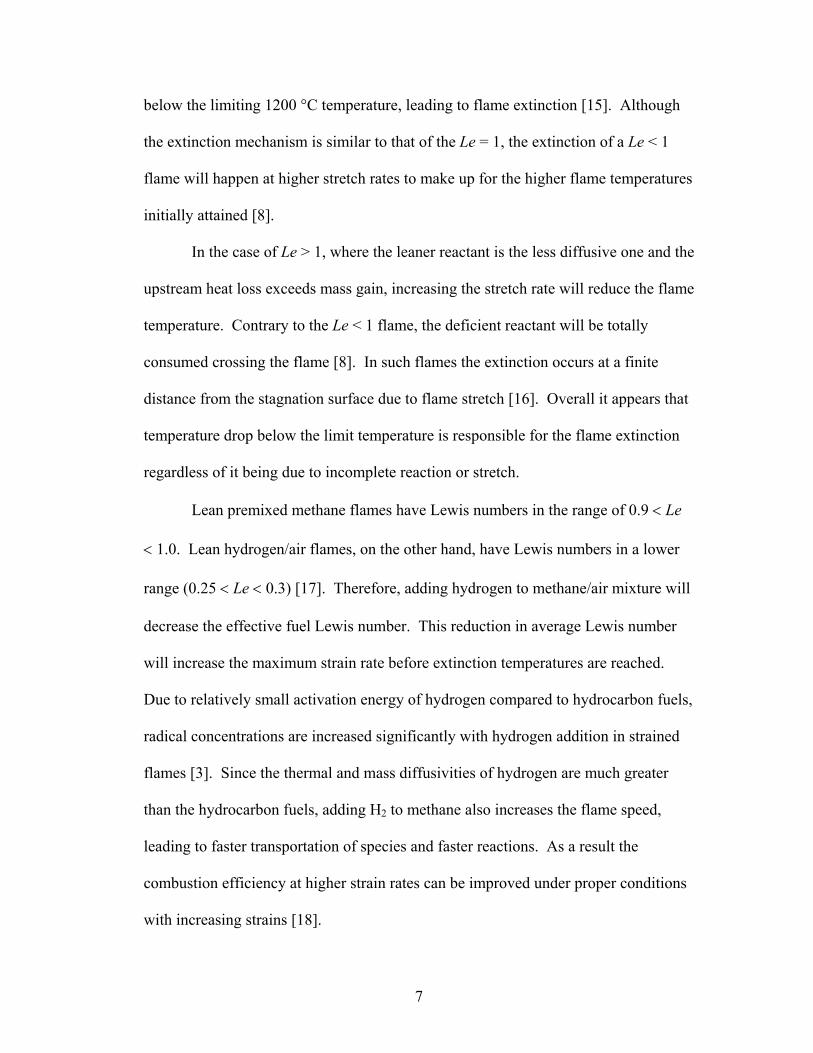
below the limiting 1200 °C temperature, leading to flame extinction [15]. Although

the extinction mechanism is similar to that of the Le = 1, the extinction of a Le < 1

flame will happen at higher stretch rates to make up for the higher flame temperatures

initially attained [8].

In the case of Le > 1, where the leaner reactant is the less diffusive one and the

upstream heat loss exceeds mass gain, increasing the stretch rate will reduce the flame

temperature. Contrary to the Le < 1 flame, the deficient reactant will be totally

consumed crossing the flame [8]. In such flames the extinction occurs at a finite

distance from the stagnation surface due to flame stretch [16]. Overall it appears that

temperature drop below the limit temperature is responsible for the flame extinction

regardless of it being due to incomplete reaction or stretch.

Lean premixed methane flames have Lewis numbers in the range of 0.9 < Le

< 1.0. Lean hydrogen/air flames, on the other hand, have Lewis numbers in a lower

range (0.25 < Le < 0.3) [17]. Therefore, adding hydrogen to methane/air mixture will

decrease the effective fuel Lewis number. This reduction in average Lewis number

will increase the maximum strain rate before extinction temperatures are reached.

Due to relatively small activation energy of hydrogen compared to hydrocarbon fuels,

radical concentrations are increased significantly with hydrogen addition in strained

flames [3]. Since the thermal and mass diffusivities of hydrogen are much greater

than the hydrocarbon fuels, adding H2 to methane also increases the flame speed,

leading to faster transportation of species and faster reactions. As a result the

combustion efficiency at higher strain rates can be improved under proper conditions

with increasing strains [18].

8

Since in most practical combustion systems the flame is exposed to turbulence

and unsteadiness, influence of oscillations on the flame structure and extinction

should also be investigated. The frequency and amplitude of the oscillations are the

two parameters that characterize this effect [7]. According to Sardi et al. [19], flame

extinction under periodic oscillations depends on the duration of imposed oscillations.

In other words, the flame may persist under oscillations even if the instantaneous

strain rates surpass steady state extinction strain rates temporarily. Exceeding the

critical strain rates may initiate flame extinction but will not be completed unless the

gradual cooling of the reaction zone during local quenching at high strain region of

the oscillation cycle forces the temperature below the limiting temperature. In this

situation the re-ignition of the flame and increase in the temperature that occurs

during low strain rate part of the oscillation cycle can no longer happen, leading to

flame extinction.

Flame temperature is a key feature for analyzing flame structure, since most

of the flame parameters such as flame velocity, thickness and extinction are

temperature dependent [1]. Although a large number of computational studies have

been conducted for strained flames, insufficient amount of high accuracy

experimental temperature data is available to verify these models. Several techniques

have been utilized to measure counterflow flame temperature.

Logue [20] used thin filament pyrometry, a visual spectrum technique to

measure temperature in a low strain stagnation diffusion flame near extinction. A 15-

µm silicon carbide fiber with nearly constant emissivity and small axial conductivity

was positioned normal to the flame surface. The flame temperature was determined

9

by relating the fiber luminescence, captured by a CCD digital camera, into a

temperature that was used to determine the gas temperature.

Temperature measurement in a near-stoichiometric methane/air mixture by

Law et al. [21] were derived from the shape of Raman spectrum and by fitting the

measured spectrum to a theoretical spectrum at a known temperature. Non-intrusive,

optical temperature measurement techniques have many advantages but they are

usually costly and require a lot of expertise in their operation. Thermocouples are

traditionally used to determine gas temperatures in the flames. In fact, temperature

profiles from other techniques such as Raman scattering are validated by comparing

with the results from thermocouples measurements [22]. Thermocouples are low

cost, easy to use, and high precision tools for measuring spatial and temporal

temperature profiles.

Tsuji et al. [16] measured temperature distributions across lean and rich near

extinction counterflow premixed flames of methane/air and propane/air to investigate

the extinction mechanism of such flames. The temperature distributions were

measured with a 0.05 mm silica-coated Pt / Pt 13% Rh thermocouple. Flame

temperature of lean methane/air had a slight increase as the velocity gradient was

increased and then decreased as the flame approached extinction limit. Flame

temperature of rich methane/air on the other hand, seemed to be almost independent

of the velocity gradient except near the extinction limit. Propane/air showed reverse

behavior in comparison with methane/air when the velocity gradient was increased.

Sato [13] used a silica-coated Pt-20% Rh / Pt-40% Rh thermocouple of 0.1

mm wire diameter to measure the temperature and investigate extinction behavior of

10

premixed stagnation flames of methane/air, propane/air and butane/air with a variety

of Lewis numbers. The thermocouple was positioned parallel to the flame to

minimize the conduction heat losses. Similar to Tsuji et al. [16] findings, opposite

situations were observed between lean and rich flames of these fuels. The studies of

Sato [13] and Tsuji [16] seem to be more focused on the behavior of flame and

pattern of changes in its temperature as the flame approaches extinction than

measuring the true flame temperature. No corrections were made for the

thermocouple radiation losses in either of these studies.

A 50-µm Pt / Pt 10% Rh thermocouple was used by Smooke [23], to measure

temperature profile in counterflow methane/air diffusion flame. The thermocouple

was coated with a layer of yttrium oxide to avoid catalytic effects. The results from

radiation corrected temperature measurements were compared with the computational

values. The discrepancy in profiles was attributed to the uncertainties in the

computational model.

Korusoy [15] measured the temperature along the stagnation plane with a bare

50-µm Pt / Pt 13% Rh thermocouple to study the effects of equivalence ratio, bulk

velocity and nozzle separation on the extinction and re-ignition of the lean premixed

opposed methane-air flame. Under-estimation of the temperature caused by

thermocouple radiation was assumed to be mostly compensated by the thermocouple

catalytic effects. Therefore the uncertainties in the absolute temperature values were

considered to be less than 3% of the mean, not affecting the observed trends.

Korusoy verified the extinction temperature acquired from a bare thermocouple by

11

comparing it to the value reported by Sato [13] obtained from a coated thermocouple

with no radiation corrections.

The instantaneous temperature traces by Luff et al. [9], in lean premixed

counterflow flames of air and methane, propane and ethylene were measured using

25-µm type R thermocouples. To reduce the catalysis effects a protective quartz

coating was applied on the thermocouples. The temperature traces were measured at

the stagnation point to study the temporal decay of flame temperature during forced

oscillations. Local extinction and re-ignition was observed by lowering the

equivalence ratio, which could also be observed following the fluctuations in the

temporal decay curves before complete extinction.

Most of the previous studies on the extinction and stability of stretched

premixed flames were based on single component fuels. Although practical

combustion systems use multi-component fuels, few studies have been conducted on

the thermal characteristics and behavior of multi-component fuels in strained lean

premixed flames. The present study will provide experimental temperature data on

highly strained lean premixed methane/air flames, with and without hydrogen

addition. Measurement of temperatures in hydrogen-doped flames is especially

challenging because of the catalytic oxidation of H2 on the thermocouple surface and

the errors that it will cause.

12

1.3 Objectives of Study

The goal of this study is to improve the understanding of lean premixed flame

behavior at high strain rates and close to extinction. Influence of hydrogen addition

on stability of lean hydrocarbon flames near extinction is evaluated. In particular the

effect of strain and its fluctuations on temperature profiles at conditions far and close

to extinction is studied. A platinum based micro-thermocouple was utilized for

temperature measurements. Thermocouple catalysis errors in these reducing flames

were lowered by coating the thermocouples. Radiation and conduction errors were

analyzed and in the case of preliminary study on oscillating flames, the temperature

measurements were compensated for thermal inertia. In addition experimental results

were compared to the predictions from an already developed reduced chemistry

model [5].

13

Chapter 2: Approach

2.1 Introduction

The temperature measurements to characterize the counterflow premixed

flames in this study were carried out along the centerline of the counterflow nozzles,

utilizing coated type R micro-thermocouples. This chapter begins with the

experimental procedures used, including the experimental setup, diagnostics, and the

measurement methodology. Then it is followed by discussion of the data analysis

method used to derive the real gas temperature from raw thermocouple data, and the

measures taken to reduce the errors.

2.2 Experimental Test Facility

2.2.1 Test Rig

The counterflow flame temperature measurements were performed in a set-up

developed by Yubin Cong [24] and improved by Roxanna Sai [25] at earlier stages of

this project. The experimental rig set-up consists of two identical nozzles positioned

in a vertical opposed flow configuration (Figure 2.1). The nozzle exit diameters are

8.5 mm and the nozzle separation distance is 0.7 ± 0.01 mm. Electronic mass flow

controllers adjust total hydrocarbon fuel, total hydrogen, and individual air flow

through the top and bottom nozzles. Identical rotameters downstream of fuel and

hydrogen mass flow controllers split the flow and send equal amounts of fuel and

hydrogen to each nozzle. Electric air pre-heaters are utilized to elevate nozzle exit

flow temperature up to 300°C. The higher initial temperatures before combustion

14

provide more stability at leaner flame mixtures and higher nozzle exit velocities.

Nozzle exit temperatures are measured by thermocouples positioned in honeycomb

flow straighteners just upstream of the nozzles. The honeycomb enhances fuel and

air mixing and reduces variations in velocity and temperature across the nozzle before

the flow exits.

Two speakers with a maximum input power of 60 Watts are placed upstream

of nozzle exits as illustrated in figure 2.1. The speakers are driven by a function

generator and an amplifier. The function generator provides a sinusoidal signal of the

desired frequency to the amplifier. When supplied with an amplified sinusoidal

voltage, the speakers impose oscillations in upstream nozzle pressure and thus nozzle

exit velocities. This flow oscillation, results in a sinusoidal variation in the stagnation

flame temperature. A multi-meter is employed to measure the input voltage to the

7.0 mmDouble Flame

AcousticSpeaker

Adaptor

CH4

H2

Air

Air Preheater

Bypass Air

Air

H2

CH4

For Cooling

Honeycomb

Thermocouple

Thermocouple

And Screen

7.0 mmDouble Flame

AcousticSpeaker

Adaptor

CH4

H2

Air

Air Preheater

Bypass Air

Air

H2

CH4

For Cooling

Honeycomb

Thermocouple

Thermocouple

And Screen

Fig. 2.1: Rig set-up

15

speakers. An empirically derived relation correlates the input voltage of the speakers

to the amplitude of velocity oscillations at the nozzle exit [5]. Small amount of cool

air that bypasses the heaters is bled into the speaker plenum to maintain the speakers

within their service temperature range.

A National Instruments (NI) data acquisition system is utilized to control the

burner operations. The user can specify the equivalence ratio, φ, the fraction of

oxygen consumed by hydrogen, α, and the desired nozzle exit velocity through a NI

LabVIEW program developed for interfacing with the data acquisition board. For the

mixtures φ is defined by the fraction of oxygen consumed by both fuel components

combined. The analog output of the data acquisition board sends an appropriate

signal to the mass flow controllers to set the desired flow rate and composition. The

nozzles exit flow temperatures are also measured and displayed so that the user can

adjust the temperatures by changing the voltage supplied to the air preheaters.

2.2.2 Traverse

An XYZ traverse system was used to obtain accurate positioning and

incremental movement of the temperature probe. The positioning system in the X

direction was utilized to move the probe horizontally out of the rig before lighting the

flame and to return the probe back to the exact previous location between the nozzles

for repeatability of the experiments. For temperature measurements at different

locations along the centerline of the nozzles, the positioning system at Z direction was

employed to shift the probe vertically. The traverse in the Y direction was used to

adjust the position of the probe at the centerline of the nozzles. Velmex positioning

16

systems (MA2509Q1-S2.5 and MA1503Q1-S1.5) in the X and Z directions were

equipped with stepping motors that could move the probe to a target position with a

10µm resolution.

The stepping motors were controlled by a Velmex VXM-2 programmable

stepping motor controller. The stepping motor controller could either be operated as

stand alone via the jog buttons on the front panel or run interactively from the

computer through a custom developed National Instruments LabVIEW program

(Appendix A) to set the control variables of the stepping motors such as: moving

direction, motor speed, motor position, zeroing motor position and the capability to

switch between stand-alone or interactive controller operation. The LabVIEW

program sends commands in the format of ASCII characters to the controller through

the RS-232 interface and displays the indexing feedback from the controller. Figure

2.2 illustrates the experimental set-up for the temperature measurement.

Traverse Thermocouple

Signal Conditioner /

Amplifier

Burner Control

Computer

Thermocouple Computer

Speaker

Amplifier

Signal Generator

Counterflow Burner

Traverse Thermocouple

Signal Conditioner /

Amplifier

Burner Control

Computer

Thermocouple Computer

Speaker

Amplifier

Signal Generator

Counterflow Burner

Fig. 2.2: Experimental set-up for temperature measurement

17

2.3 Diagnostics

2.3.1 Thermocouple Support Design

Instantaneous local temperatures were measured using a type R (Pt/Pt–

13%Rh) thermocouple of 50 µm wire diameter with a bead of approximately 100 µm

in diameter. The high melting point of type R thermocouple (2023 K) makes it a

suitable probe for the range of temperatures in this study and the small size of the

probe provides high resolution with minimal disturbance of the flame. Low response

time and reduction in the radiation losses are other benefits of the small size of the

probe. As a preliminary design the thermocouple bead was suspended between two

0.8 mm diameter, single bore ceramic supports separated by 20 mm (Figure 2.3). The

supports were fixed within a modified thermocouple connector. Since in this design a

considerably long portion of the thermocouple wire was exposed to the surrounding

environment, thermal expansion and bending of the thermocouple wire in the flame

region caused uncertainties in defining the exact axial location of the bead.

Ceramic Insulation

Probe Supports

Modified Jack

20 mm

125 mm

Pt / Pt-13%Rh (dw = 50 µm)

Support Adjustment

Fig. 2.3: Thermocouple support [27]

18

As shown in the snapshots in the figures 2.4.a to 2.4.c, when the thermocouple

position changed from the cooler upstream region of flame to the high temperature

flame region, the tightly drawn wire expanded and moved. In such condition the wire

has a low tensile strength and pulling the wire, as an effort to straighten it, will only

cause the wire to break. As a result a change in the support design was necessary.

In the new design a smaller length of thermocouple wire (~ 9 mm) was

exposed. The exposed wire was shaped into a flat semicircular form. The remaining

thermocouple wires were insulated within a single 1.1 mm diameter twin bore

ceramic cylinder, which in turn was housed within a nickel alloy protective tube

(Figure 2.5). Probe-induced perturbations are reduced in this single support design.

Ceramic InsulationProbe Support

Miniature Connector

125 mm

Pt / Pt-13%Rh (dw = 50 µm)

Fig. 2.5: Thermocouple single support design

(a) (b) (c)

Fig. 2.4: Thermocouple wire expansion in flame

19

Although in this design the shorter length of exposed wire significantly

reduces thermocouple positioning errors caused by thermal expansion, conduction

losses may not be negligible anymore. Ceramic insulation with much larger surface

area than the exposed thermocouple wire loses more heat from radiation. As a result,

the insulated section of the thermocouple wire has a lower temperature than the

exposed part, which increases the heat conduction through the wires. Dependence of

conduction heat loss on the length of the wire will be discussed in more details in §

3.2.2. To quantify and account for the conduction heat loss in deriving the gas

temperature from the thermocouple bead temperature, the temperature of the

insulated wire should be known.

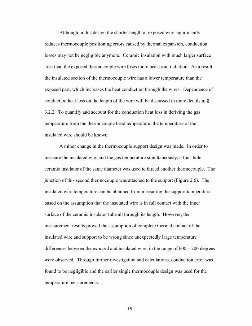
A minor change in the thermocouple support design was made. In order to

measure the insulated wire and the gas temperature simultaneously, a four-hole

ceramic insulator of the same diameter was used to thread another thermocouple. The

junction of this second thermocouple was attached to the support (Figure 2.6). The

insulated wire temperature can be obtained from measuring the support temperature

based on the assumption that the insulated wire is in full contact with the inner

surface of the ceramic insulator tube all through its length. However, the

measurement results proved the assumption of complete thermal contact of the

insulated wire and support to be wrong since unexpectedly large temperature

differences between the exposed and insulated wire, in the range of 600 – 700 degrees

were observed. Through further investigation and calculations, conduction error was

found to be negligible and the earlier single thermocouple design was used for the

temperature measurements.

20

2.3.2 Thermocouple Coating

In this study, platinum-based type R thermocouples were used for temperature

measurement due to their high service temperature. Catalytic reactions in reducing

combustion environments will produce inaccuracies in platinum-based thermocouples

temperature readings. In order to reduce this effect, a non-catalytic coating is applied

on the thermocouple bead and wires. Some of the factors taken into account for

choosing the coating were: having a similar thermal expansion coefficient as the wire

to avoid cracking when exposed to heat, stability of the coating, and ease of

application. In § 3.2.4 the catalytic effect will be discussed in more details.

Several types of coating were tested and Aremco Ceramabond 569-VFG gave

the best results for our application. This aluminum oxide/potassium silicate coating

was recommended by Burton et al. [26] as a non-toxic coating that lasts for several

hours of use before degradation. According to the manufacturer, Ceramabond 569

adheres well to metals and can be used at temperatures as high as 1900 K. The best

method to apply a thin layer of coating was found to be using a fine-tip brush. To

make sure that the thermocouple bead and exposed surfaces of the wires were

completely covered with the coating, the thermocouple was inspected using a high

Fig. 2.6: Measurement of thermocouple support temperature

1.2 mm 0.25mm Support Probe (dw=50 µm)

Gas Probe (dw = 50 µm)

21

magnification optical microscope (Figure 2.7). This inspection was done before and

after exposure to heat to make sure that the coating performance was satisfactory.

The coated thermocouple bead under different magnifications is pointed out with

arrows in this figure. The coating increased the measurement junction diameter to

200 µm.

2.3.3 Data Acquisition System

National Instruments 5B40-05 signal conditioner with a 10 kHz bandwidth

was used to amplify the thermocouple millivolt signal by a factor of 100 and to filter

the background electrical noise. The wide bandwidth makes the signal conditioner

suitable for measuring signals that change rapidly with time. The amplified analog

signal is interfaced to a 16 bit National Instrument PCI-MIO-16XE-50 data

acquisition board and converted to digital data. The DAQ board is mounted within a

PC running a custom National Instruments LabVIEW program (Appendix A). The

program converts the digitized voltages to actual temperatures via a standard

polynomial equation and displays the temperature signature for inspection before

saving the data to disk. Moreover, the program provides statistical temperature data

such as mean, minimum, maximum, and standard deviation. The data acquisition

Fig. 2.7: Thermocouple coating microscopic images

22

parameters such as frequency and sampling time can be easily changed in the

LabVIEW program control panel.

2.4 Temperature Measurement Methodology

Thermal behavior of close to extinction premixed flames of pure methane and

hydrogen doped methane under both steady-state and oscillatory upstream velocities

are investigated in this study. In order to consistently and accurately study the effects

of strain and hydrogen doping on the thermal characteristics of methane flames,

important parameters were determined. The experiment matrix was designed so that

certain parameters were kept constant while effects of the other variables were

evaluated.

The hydrogen doped mixtures are characterized by equivalence ratio, φ,

defined as the fraction of O2 consumed by both fuel components combined and by α,

the fraction of O2 consumed by H2. The thermocouple service limit, imposed by its

melting point was an important parameter in selection of φ and α. In the current study

the mixture φ was kept constant at 0.65 and α ranged from 0.0 to 0.1, which was

found to be adequate to observe impacts of H2 on the methane flame [25].

The extinction strain rate is a function of equivalence ratio, fuel composition,

and inlet temperature. In order to find the extinction strain rate of the steady flame, φ

and α are kept unchanged. The velocity of the fuel and air combination leaving the

nozzles with a 300°C exit temperature is slowly increased in 0.1 m/s increments after

thirty seconds of stable operation. At the inlet velocity that the flame extinction

occurs, the corresponding global strain rate, κext, is obtained by dividing the mean exit

23

flow velocity by half of the separation distance between nozzles. Thermal behavior

of the steady flame at κmean / κext = 0.85 and κmean / κext = 0.6 corresponding to close

and far from extinction conditions respectively, was investigated for each fuel

mixture.

Type R thermocouples of 50 µm wire diameter were used in pure methane and

hydrogen-doped methane flames because of their high melting point (2023 K) [28].

The thermocouples were coated to minimize the catalytic effect. This coating

increased the bead diameter to 200 µm. The temperatures were measured along the

centerline of the nozzles with 0.25 mm increments at positions away from the flame

and 0.125 mm increments at positions close to the flame. Exactly 10,000 data points

separated by 1 ms were sampled at each position at the steady conditions and at the

oscillating conditions 300,000 data points separated by 0.1 ms were sampled at each

position.

24

Chapter 3: Data Analysis

3.1 Introduction

The temperature measured by the thermocouple may differ from the real gas

temperature. There are several reasons for the difference. Radiation and conduction

losses, thermal inertia, non-uniform thermocouple heating, catalytic effects, and the

effect of probe intrusion on the flame are major factors affecting the reading of the

thermocouple. The relative effect of these factors depends not only on the properties

of the thermocouple itself, but also on the gas phase properties and whether the

measurement is done at steady or transient condition. In order to derive a true gas

temperature from the thermocouple measurement, a good understanding of all major

sources of error is required. In this section various possible sources of errors

encountered in thermocouple measurements and our approach to eliminate or

minimize these errors are discussed.

Comparison of the experimental data with the results from an already

developed computational model [5], the accuracy of which has been verified by

comparison with a non-intrusive measurement temperature data from another source

[21], helped us to get an estimate of the importance of some of the errors which could

not be quantified otherwise. The model solves for flow velocity, temperature, and

species mass fractions along the central axis of the flow within a cylindrically

symmetric counterflow premixed flame. In § 3.7 more details about the validity of

the model will be discussed.

25

3.2 Thermocouple Probe Heat Transfer

The energy balance on the thermocouple bead is a combination of convection,

radiation, conduction heat transfer, and catalysis induced heating [22,27] as shown in

figure 3.1. The energy balance on the thermocouple bead can be expressed as

0=++++ storcatcondradconv QQQQQ &&&&& (3.1)

where Q& is the net rate of heat transfer. In the steady state conditions the rate of

change of energy storage in the thermocouple, storQ& , is equal to zero. Since the

purpose of using the thermocouple is measuring the local gas temperature, it is

preferred to have convection as the major source of heat transfer to the thermocouple.

3.2.1 Convection

Modeling of the convective heat transfer around a thermocouple is not an easy

task and involves some uncertainties. Selection of the appropriate correlation for

calculation of the Nusselt number and estimation of the properties of the gas

surrounding the thermocouple, especially its thermal conductivity are the two main

Convection

Radiation

Conduction

Catalysis

Energy Storage in the bead

Probe Support

Convection

Radiation

Conduction

Catalysis

Energy Storage in the bead

Probe Support

Fig. 3.1: Heat transfer modes in thermocouple

26

challenges for accurate modeling [22]. The heat gained by the thermocouple, at

temperature Tb, is convected by the gas at Tg which, is described by:

)( bgsconv TThAQ −=& (3.2)

where, As is the bead surface area, and h is the convective heat transfer coefficient of

the flow over the thermocouple junction defined as dkNuh = . k is the thermal

conductivity of the gas, Nu is the Nusselt number, and d is the bead diameter.

The Nusselt number correlation is usually chosen based on the thermocouple

bead geometry, being spherical or cylindrical. The commonly used correlation for

forced convection over a spherical geometry is proposed by Whitaker [29] for 3.5 <

Re < 76×104 and 0.71 < Pr < 380.

( ) ( ) 414.03221, PrRe06.0Re4.00.2 sddsphdNu µµ∞++= (3.3)

The dimensionless groups in this equation are Reynolds number, µρ udd =Re , and

Prandtl number, kcpµ=Pr ; where u is the velocity of flow over the thermocouple,

and µ, ρ, and cp denote the dynamic viscosity, density, and the specific heat of the gas.

All properties except the dynamic viscosity at surface, µs, are evaluated at T∞. Ranz

and Marshall recommended another expression for spherical geometry at the

Reynolds numbers range of 0 < Re < 200, in the form of [30]:

3121, PrRe6.00.2 dsphdNu += (3.4)

Many different Nusselt number correlations have been introduced for the

cylinders. The Collis and Williams correlation is frequently used for flow over

cylindrical geometries for the Reynolds numbers in the range of 0.02 to 44 [29]:

45.0, Re56.024.0 dcyldNu += (3.5)

27

Kramer’s correlation is for a wider range of Reynolds number from 0.01 to 10,000

expressed as [22]:

21312.0, RePr57.0Pr42.0 dcyldNu += (3.6)

The difference in the value of Nusselt number obtained from the spherical and

cylindrical correlations are evident just by comparing them at Reynolds number close

to zero. At this condition Nusselt number equals 2.0 for a sphere, while Nu ~ 0.3 for

a cylindrical geometry. Figure 3.2 shows how the selection of the Nusselt number

correlation will result in different values.

As mentioned earlier, the choice of Nusselt number correlation is

conventionally based on the geometry of the bead being spherical or cylindrical or a

qualitative evaluation of the diameter of the thermocouple bead relative to the

diameter of the thermocouple wire. Since the diameter of the bead is usually 1.5 – 3

Fig 3.2: Calculated Nusselt numbers at a 900 K near flame location (Methane flame of φ = 0.65 and κmean / κext = 0.8)

Coated Thermocouple

28

times the diameter of the wire, the spherical correlations are conventionally used for

the thermocouples. The microscopic pictures of the thermocouples used in this study

clearly showed the spherical geometry of the bead and also its diameter being at least

two times the diameter of the wire. Therefore Whitaker correlation (eq. 3.3) was used

to derive the Nusselt number as marked on figure 3.2.

Correct estimation of the properties of the gas surrounding a thermocouple is

also an important factor in accurate calculation of gas temperature from the

thermocouple measurements. Local gas properties such as viscosity, thermal

conductivity, density, and the specific heat are required for calculation of the Nusselt

number and convective heat transfer coefficient. Since evaluation of local gas

properties is a strenuous task, properties of air or nitrogen at the local gas temperature

are often used to approximate the gas properties [22]. In this study the properties of

air at local temperature and the computational model velocities at each thermocouple

position along with heat transfer correlations were used to calculate the Nusselt

number, Nu, and the convective heat transfer coefficient, h.

29

3.2.2 Conduction

The conduction of heat between the thermocouple junction and the lead wire

and support can be an important source of error in the temperatures measured by the

thermocouple. The amount of conduction heat loss through the thermocouple wire is

directly proportional to the longitudinal temperature gradients in the wire [22,31], and

is expressed by Fourier’s law:

xTAkQ wwcond ∆

∆=& (3.7)

in which, condQ& is the conduction heat transfer rate, kw is the thermal conductivity of

the thermocouple wire, Aw is the area through which heat is being conducted and

xT ∆∆ is the temperature gradient through the length of the thermocouple wire. This

gradient could be can be a result of temperature gradients in the gas. To reduce the

conduction errors in the presence of such gradients, the thermocouple is aligned in a

way that the length of the wire is along an isotherm.

The amount of conduction heat loss also depends on the length of the wire

between the junction and support. To illustrate the conduction error corresponding to

a given length of thermocouple wire, an energy balance is performed on the

thermocouple wire. The analysis is simplified by assuming convection and

conduction as the only sources of heat transfer around the thermocouple. Considering

one-dimensional conditions in the longitudinal direction, monotonic temperature

distribution, and uniform diameter, D, the temperature distribution along the

thermocouple wire can be derived as [30]:

ggsupp TmL

xLmTTxT +−

−=cosh

)(cosh)()( (3.8)

30

where x is the distance from the support, T(x) is the wire temperature at position x,

Tsupp is the support (lead wire) temperature, Tg is the gas temperature, and m is

defined as kDhm 4= . h is the convection heat transfer coefficient and L is half

length of the exposed wire. The assumption of uniform diameter is only made to

simplify the analysis since the bead is normally spherical and its diameter is 1.5 – 3

times the diameter of the wire. From this equation, the temperature at half length (at

the junction) of the exposed wire, and the conduction error defined as Tg - T(x) can be

calculated. Figures 3.3 and 3.4 illustrate how the magnitude of conduction error

varies with the length of a 50 µm thermocouple wire. Figure 3.3 shows the

conduction cooling error defined when Tg - T(x) > 0 and figure 3.4 shows the

conduction heating error when Tg - T(x) < 0.

Fig. 3.3: Variation of conduction cooling error with thermocouple wire length in methane flame (φ = 0.65, α = 0.1 and κmean / κext = 0.6)

Thermocouple used in this study

31

The thermocouple support is typically cooler than the thermocouple wire and

junction as a result of more radiation loss to the surrounding [22], which may cause

considerable conduction heat loss from the thermocouple wire and junction to the

cooler support. Figure 3.3 illustrates this situation when the thermocouple is at a

position inside the counterflow flame. As is evident in this figure, the conduction

cooling error is more significant if the wire has a smaller length. Using longer

lengths of thermocouple wire can reduce the conduction losses. In special cases,

such as when the thermocouple support is closer to the flame than the thermocouple

wire, for example the positions where the thermocouple wire is outside and parallel to

the counterflow flame, the support will be closer to the flame because of its larger

size and will conduct heat to thermocouple junction (Figure 3.5). Here also the

amount of conduction error depends on the wire length (Figure 3.4).

Wire Length (mm)

Con

duct

ion

Hea

ting

Erro

r(K

)

0 5 10 15 20 25-30

-25

-20

-15

-10

-5

0

Near FlameOutside Flame

Fig. 3.4: Variation of conduction heating error with thermocouple wire length

in methane flame (φ = 0.65, α = 0.1 and κmean / κext = 0.6)

Thermocouple used in this study

32

Fig. 3.5: Temperature difference between thermocouple and support

The values used for Tsupp in these figures were from the support temperature

measurements, which as mentioned in § 2.3.1 were over-predicting the difference

between the exposed wire and insulated wire temperatures. Even with over-

prediction of the conduction error, the magnitude of the error is insignificant for the 9

mm wire length used in this study.

In high velocity field it is more desirable to use short lengths of thermocouple

wires to have a robust probe. However, according to Bradley and Mathews [32], if

the length to diameter ratio, l/dw, of the wire is below a minimum value such as 200,

the conduction heat loss can be significant. Petit et al. [33], suggested that a better

criterion was to use wires of length l such that l/lc > 10, in which lc is the

characteristic length defined as convwwc hdkl 4= . This criterion accounts for both

the characteristics of the flow and of the sensor.

Values obtained from applying Petit criterion to the thermocouples used in

this study with the exposed wire of 9 mm length and wire diameter of 50 µm at

different locations in flame and out of flame, are in the range of 17 - 21 for the l/lc

Counterflow flame

ThermocoupleThermocouple support

33

ratio which is above the recommended value of 10. Overall, the conduction error is

considered negligible in this study.

3.2.3 Radiation

In general, the temperature of a thermocouple is affected by radiative heat

exchange between its outer surface and the surroundings. The amount of this heat

transfer is given by [30]:

)( 44surrbrad TTAQ −= σε& (3.9)

where σ is the Stefan-Boltzmann constant )KmW1067.5( 428 ⋅×= −σ , ε is the

emissivity of the thermocouple surface, A is the surface area of the junction, Tb is the

junction temperature, and Tsurr is the surrounding surfaces temperature. This is a

simplified analysis assuming the effect of radiation from other sources negligible and

also constant value for Tsurr .

Radiation losses are the most significant cause of error in the thermocouple

temperature data especially at temperatures above 1000 K [34]. Assuming negligible

conduction losses and catalytic effects by using sufficiently long thermocouple wires

and applying non-catalytic coating on the thermocouple wire and junction, if

required, energy balance of eq. 3.1 on the thermocouple junction can be expressed as:

0=+ radconv QQ && (3.10)

which may be rewritten as:

)( 44surrbbg TT

hTT −+=

εσ (3.11)

34

Performing radiation corrections on the thermocouple measurements is not an

easy task. Emissivity of the thermocouple, choice of Nusselt number correlations, the

local gas properties, the size of the thermocouple, and thermal radiation sources

surrounding the thermocouple are some of the factors that could change the amount

of the radiation correction.

Emissivity, which is a radiative property of the thermocouple surface,

strongly depends on the surface characteristics, i.e. material and finish, which may

change by exposure to combustion environment [30]. Moreover, emissivity varies

with temperature and wavelength [35]. For instance it has been found that in the

temperature range of 600-900°C, emissivity of Pt-10%Rh wire can change as much as

40% [31]. Unfortunately, limited experimental data on emissivity of common

thermocouple wires and non-catalytic coatings is available in literature.

An infrared camera was utilized to measure the emissivity of coated type R

thermocouple. A thermocouple heating/cooling circuit that was originally designed

for the time constant measurement (§ 3.6) is used for this measurement. During the

heating cycle, DC heating current from a power supply flows into the thermocouple

and heats it up. When the heating current is turned off, the peak temperature

measured by the thermocouple just at the start of cooling cycle is recorded.

Simultaneously, the infrared image of the thermocouple is taken and the peak

temperature is determined. Since the emissivity value on the infrared camera system

should be calibrated, in most cases the temperature from IR camera does not agree

with the temperature from the thermocouple. This value should be adjusted on the IR

system until the measurement function displays the same temperature as the

35

thermocouple. This adjusted emissivity is considered the emissivity of the

thermocouple. The measurements were performed at low, medium, and high ranges

of temperatures. Emissivity of the coated type R thermocouple in the temperature

range of 600 – 1600 K varied in the range of 0.7 – 0.4.

The choice of the Nusselt number correlation will also affect the amount of

radiation correction for the thermocouple measurements since the thermocouple

radiation correction is inversely proportional to the convective heat transfer

coefficient and Nusselt number( khdNu = ). Figure 3.6 shows this effect when

results from the correlations for spherical geometry are compared to cylindrical

correlations.

As mentioned in § 3.2.1, a number of local gas properties are needed for

calculation of Nusselt number and heat transfer coefficient. However, the local gas

Fig. 3.6: Calculated radiation correction using Nusselt number correlations at a 900 K near flame location (Methane flame of φ = 0.65 and κmean / κext = 0.8)

Coated Thermocouple

36

properties are not usually known and may vary. In addition, there are some

uncertainties in the Nusselt number correlations, which are based on experimental

data [22].

Another important factor in the amount of radiation correction is the

thermocouple size. The general recommendation for reducing the radiation losses is

to use the smallest possible thermocouple junction and wire. Rewriting the equation

3.11, by utilizing definition of Nusselt number, shows the effect of thermocouple

size:

)( 44surrbbg TT

kNudTT −+=εσ (3.12)

All Nusselt number equations correlate with Re1/2, therefore with d1/2. At low

Reynolds numbers typical of the high temperature thermocouple measurements, the

effect of Reynolds number on Nusselt number is considerably small. As a result, at

these conditions the radiation corrections vary directly with thermocouple wire and

bead size [22]. Figure 3.7 shows the effect of wire size on the amount of radiation

errors at different thermocouple locations. Since radiation is proportional to 4T , it is

clear that at high-temperature positions inside the flame a thermocouple bead will

radiate more compared to low-temperature positions near or outside the flame.

Moreover, the smaller convective heat transfer coefficient at locations inside the

flame, contributes to larger radiation losses.

37

The thermal radiation sources surrounding a thermocouple such as the hot

combustion gases and the flame may also affect the thermocouple measurement. This

effect depends on the temperature, composition, concentration of emitting species,

and path length [36]. In the absence of soot particles as in the non-luminous flames,

CO2 and H2O are considered as the main emissive species in combustion products

[37,38]. Using Hottel data on emissivities, Drysdale [36] illustrates that non-

luminous flames have very low emissivities. Since the thickness of lean counterflow

flames especially at close to extinction conditions is very small (~ 1mm), effect of

radiation from hot gases on the thermocouple measurement is considered negligible.

Wire Diameter (µm)

Rad

iatio

nLo

ss(K

)

0 50 100 150 2000

50

100

150

200

250

Outside FlameNear FlameInside Flame

Fig. 3.7: Effect of thermocouple wire diameter on the radiation loss (Methane flame of φ = 0.65 and κmean / κext = 0.8)

38

3.2.4 Catalysis

In high-temperature combustion environments, platinum-based type R

thermocouples are commonly used due to their high service temperature. Unoxidized

fuel molecules and pyrolysis products in such environments, particularly those

containing hydrogen use platinum as a catalyst for reaction and recombination. These

recombination reactions can start at temperatures below 400°C [39]. At low

temperatures, principally H2 is participating in the reactions because its approximate

lightoff temperature on platinum is between 100-150°C. Above 550°C, methane

becomes active and thus CH4 and any pyrolysis products can be oxidized on platinum

[40]. If there is enough hydrogen in the gas flow to heat up to methane lightoff

temperatures, even at low temperatures very high thermocouple temperatures can be

read.

Once chemical reactions are initiated they produce heat, causing error by

raising the temperatures measured by the thermocouple [22,26,31,34]. Catalytic

activity is highest in the pre-flame zone and the reaction zone and depends on

concentration of un-burned fuel, local mean temperature, time at that temperature,

and on the hydrogen content of the fuel [31].

The best method for reducing or eliminating catalytic effect is to coat the

thermocouple with a non-catalytic material, which must also be impermeable to flame

gases. Three common types of coatings used are: silica-based coating, beryllium

oxide/ yttrium oxide ceramic, and alumina-based ceramic. Silica-based coating can

be applied as a thin coating with relatively low emissivity. However, it has been

found to be very fragile [26] and to react with hydrogen at temperatures above

39

1100°C. The BeO/Y2O3 coating also forms a thin coating but is not very stable, has

large emissivity, and is highly toxic. Alumina-based ceramic coatings have become

more common in recent years because of their stability at high temperature. Yet, due

to their viscous nature, they form a thicker coating.

Although coating reduces the catalytic effect, it increases the thermocouple

diameter, the response time of the thermocouple, and the radiation losses. It also

changes the convective and conductive heat transfer of the thermocouple. Therefore,

in order to get the best results a very thin layer of coating should be applied. Since

the coating changes the heat transfer properties of the thermocouple, it is difficult to

quantify the effect of catalysis. However, a qualitative comparison of type R

measurements with type K thermocouple measurements, at positions where the

temperatures were below the melting point of type K thermocouple, showed

satisfactory reduction in the catalytic effects after coating the thermocouple.

3.3 Non-uniform Thermocouple Heating

Another source of error in the thermocouple measurements is the non-

uniformity of temperature distribution within the thermocouple junction and wires.

This non-uniformity will reduce the sensitivity of the thermocouple [41] or cause

conduction errors.

Physical and thermal properties of the thermocouple itself may be the reason

for such non-uniform heating. The Biot number, defined by khLBi = , where L is

characteristic length, h is convective heat transfer coefficient, and k is the thermal

conductivity of the wire, provides a measure of rate of convective heat transfer to the

40

thermocouple bead and wires relative to radial thermal conduction within the

thermocouple [22]. If Bi << 1, the temperature drop in the thermocouple junction

relative to the temperature difference between the thermocouple surface and the

surrounding gas will be very small and at this condition it is reasonable to assume

uniform temperature distribution across the thermocouple [30].

As mentioned in § 3.2.2, in the presence of temperature gradients in the

combustion gas, the thermocouple should be aligned along an isotherm to minimize

the conduction errors. Yet in some flame configurations the temperature gradients

are so large that can produce internal temperature gradients even in small diameter

thermocouples with Bi << 1. For instance, the temperature gradient across the

thermocouple bead in the counterflow methane flame of the present study (φ = 0.65,

Uinj = 7 m/s, κ/κext = 80%) could be as large as 600 K. According to Weckmann [41]

at this condition the temperature measured by the thermocouple is either assumed to

be the highest temperature at the junction or an average temperature of the junction.

3.4 Thermocouple Positioning

Since temperature measurements are tied to a position, an important issue with

the thermocouple measurements is the errors introduced by movement or vibration of

the thermocouple. These movements can be generated from flaws in the support or

the positioning system, or can be a result of alternating thermal expansion and

contraction of the thermocouple wire as it moves from one temperature region to

another, especially at regions with high temperature gradients [34]. Utilizing a robust

41

support and positioning system and minimizing the length of the fine thermocouple

wire (§ 2.2.2 and 2.3.1) were measures taken to reduce the errors in this study.

3.5 Probe-induced Disturbances

Thermocouple intrusion in the gas stream may cause the measured

temperatures to be different from what is characteristic of undisturbed stream.

According to Fristrom [34], the aerodynamic effect of thermocouple intrusion on the

flame will produce a velocity-deficient wake that deforms the flame and displaces the

isothermal surfaces in the flow that are flat otherwise (Figure 3.8). This deformation

moves the flame closer to the thermocouple. As a result, the thermocouple tends to

record higher temperatures than what is characteristic of that position in an

undisturbed flow. Minimizing the size of the thermocouple can reduce this error.

Fig. 3.8: Probe-induced disturbances [34]

Isothermal surface displacement

Thermocouple

Wake

Flow direction

42

3.6 Thermal Inertia

When measuring high-frequency temperature fluctuations, thermal inertia of

the thermocouple will cause a delay in the response of the probe to the input heat

flux. Thus, the thermocouple output will be attenuated and phase-delayed. This

temporal lag is characterized by the thermocouple time constant and should be

compensated to recover the fluctuations of gas temperature from the measured data

[27,31,32].

The time constant of the thermocouple is defined as the time the probe takes

to respond to the changes in its surrounding temperature. Assuming conduction

losses from the thermocouple as well as catalytic reactions on the probe surface to be

negligible, the energy balance of the equation 3.1 on the thermocouple bead can be

rewritten as:

0=++ storradconv QQQ &&& (3.13)

or [27],

))(()(

)()( 44surrb

bbg TtT

dttdT

tTtT −++= γτ (3.14)

where τ is the characteristic response time or time constant of the thermocouple, and γ

is the ratio of radiative effects to convective effects as shown by:

b

pb

hAcm

=τ (3.15)

hεσγ = (3.16)

Equation 3.15 shows that the time constant of the thermocouple is not only

related to the physical properties of the thermocouple, i.e. the mass of the

43

thermocouple junction, mb, the specific heat, cp, and the surface area of the junction,

Ab, but also depends on heat transfer coefficient of the flow, h. Determining the value

of cp and h is difficult since they are dependent on local temperature, velocity, and

composition of the flow [31]. Moreover, changes in the geometrical shape of the

bead after coating introduces more uncertainties in determining the exact surface area,

Ab, of the bead.

A more conventional method to directly determine the time constant is to use

the temperature step change method [27]. In this method τ is found from the response

time of the thermocouple to a step change in the temperature of the probe. For a

thermocouple system where radiation losses are negligible, τ can be defined as the

time taken for the thermocouple temperature to decay to 1/e of this step change as

shown in figure 3.9 because the governing equation is first order with respect to

temperature. In this method a DC electrical current heats the thermocouple junction

Fig. 3.9: Average temperature decay for calculation of the time constant

44

above the local flame temperature. The over-heat temperatures are kept relatively

small K100K50 <∆< T so it does not significantly affect the local flame

characteristics. The heating current is then switched off to create a step change from

the overheat temperature to the local flame temperature. The thermocouple

temperature subsequently decays to this local flame temperature. The heating and

cooling cycles are repeated hundreds of times and the average time constant is found

from ensemble averaging of the decay cycles. An average decay curve from 100

heating/cooling cycles is shown in figure 3.9. The theoretical exponential decay

curve corresponding to the measured time constant is also displayed. As the figure

shows, average decay curve is in reasonable agreement with the theoretical

exponential decay, which validates the first-order assumption of the system.

Average local time constant is measured using a switching circuit designed to

trigger the heating/cooling cycles at the appropriate times. The set-up for the

measurement is shown in figure 3.10. Two fast response solid-state relays with

maximum on/off time of 50 µs are employed to isolate the heating and cooling cycles.

During the heating cycle, a TTL signal from the DAQ computer to the heating circuit

relay closes the circuit and DC heating current from a power supply flows into the

thermocouple. When the heating current is turned off, another TTL signal triggers

the cooling circuit relay and thermocouple voltage decay is collected by the amplifier

and the data acquisition board. The number of heating cooling cycles, the time period

for each cycle, and the frequency of thermocouple data collection are controlled by a

LabVIEW program developed for this purpose. An IDL program is also developed to

average the decay cycles and calculate the time constant for each set of

45

measurements. Temperature step change of the average decay curve is calculated

from the initial temperature as the maximum and the average of the last 1/10 of the

data points as the stable minimum temperature of the decay curve. For the coated

type R thermocouple in the temperature range of 1070 K < T < 1770 K time constants

in the range of 100 ms < τ < 320 ms were obtained. The measured τ was

unrealistically large. Ultimately, the velocities from the analytical model [5], were

used along with the heat transfer correlations to determine the convective heat

transfer coefficient, h at each measurement location to obtain the time constant.

With the knowledge of average time constant value, the thermal inertia of the

thermocouple can be compensated. However, compensation of thermal inertia based

on equation 3.14 involves calculation of time derivative of temperature, which may

be inaccurate when dealing with discrete values. In order to avoid errors in the

calculation of the derivative, differentiation of the transient term is performed in the

HeatingDC supply

+-

TTL

Relay 1 (Heating cycle)

Control3

4 21 +-Load

+-

TTLControl

Relay 2 (Cooling cycle)+

-213

4

ThermocoupleLoad

Computer

Amplifier

DAQ Board

HeatingDC supply

+-

TTL

Relay 1 (Heating cycle)

Control3

4 21 +-Load

+-

TTLControl

Relay 2 (Cooling cycle)+

-213

4

ThermocoupleLoad

Computer

Amplifier

DAQ Board

Fig. 3.10: Experimental set-up for measuring response time of the probe

46

frequency domain using Fourier transform [27]. Thus, the gas temperature can be

expressed as:

[ ] ))(()(FFT)()( 44-1surrbbbg TtTTjtTtT −++= γωτω (3.17)

where Tb(ω), is the Fourier-transformed temperature (calculated with Fast Fourier

Transform), ω is the frequency, and FFT-1 is the inverse Fast Fourier Transform. A

program written in IDL [27] is used to digitally compensate for thermal inertia and

radiation effects at the thermocouple junction. Assuming negligible radiation effect,

the compensation program was applied on a simple sinusoidal temperature signal to

show the difference between uncompensated and compensated signals. As illustrated

in figures 3.11 and 3.12, uncompensated signal is attenuated and phase-delayed

compared to compensated signal. The attenuation and phase difference depends on

the frequency of temperature oscillations and the time constant of the thermocouple.

Figure 3.11 demonstrates how for a certain value of time constant, larger frequency of

temperature fluctuations will results in larger error in uncompensated data. Also

comparison of figures 3.11 (a) and 3.12 (a) or figures 3.11 (b) and 3.12 (b) shows

how larger time constant will result in larger attenuation and phase delay. It may be

concluded that compensation process compensates for amplitude and phase delay in

raw data.

47

(a) Frequency = 15 Hz

(b) Frequency = 60 Hz

Fig. 3.11: 100 ms of uncompensated and compensated sinusoidal signal at τ = 15 ms

48

(a) Frequency = 15 Hz

(b) Frequency = 60 Hz

Fig. 3.12: 100 ms of uncompensated and compensated sinusoidal signal at τ = 30 ms

49

3.7 Measurement Validation

The thermocouple data were not compared directly with other experimental

results since no data with similar experimental conditions to our experiments were

found. Instead, our data were compared with a FORTRAN-based computational code

adapted from CHEMKIN-based premixed code that was shown to predict the flame

behavior accurately [17,25]. The model is used to calculate the flow velocity,

temperature, and species mass along the central axis of the nozzles within a

cylindrically symmetric counterflow premixed flame. The model can predict the

behavior of methane flame with and without hydrogen doping as a function of strain

rate.

In this section, first it is established that the computational results can

accurately simulate the thermal behavior of the strained flame at the conditions used

by another independent experimental study. Next, there is a discussion on how the

uncertainty in parameters such as equivalence ratio or strain rate will cause

uncertainty in the choice of comparable computational data.

3.7.1 Model Quality Assessment

The experimental condition of an independent study by Law et al. [21] was

simulated and the computed temperature profile was compared to the experimental

data from that study. The experiments were conducted in a counterflow configuration

with nozzle diameter of 14 mm at separation distance of 11 mm. The near-

stoichiometric (φ = 0.95) methane/air mixture of Law’s study was diluted by nitrogen

to achieve extinction strain rates which were within the capability of the flow system.

50

The temperature measurements were derived from the shape of Raman spectrum. A

comparison between experimental and computed temperature profile at one of the

experimental conditions in Law’s investigation is illustrated in figure 3.13. Although

the measurements were performed at much lower strain rates (< 400 s-1) compared to

strain rates of the present study in the range of 2500 s-1 < κmean < 6700 s-1 and at larger

nozzle separation compared to the present study, the computed results are found to

have reasonable agreement with the experimental data, hence supporting the validity

of the computational model for the simulation of strained flames.

3.7.2 Uncertainty in Experimental Parameters

As mentioned earlier, the experiments of this study have been conducted at a

specific equivalence ratio and strain rate. However, there are some uncertainties in

the experimental value of these parameters which can be due to instrumentation e.g.,

Fig. 3.13: Comparison between computed profiles and Raman scattering temperature profiles (Case C, κmean / κext = 0.5, κext = 400 s-1) [21]

51

from the mass flow controller, the heaters, leakage of un-burned fuel or from facility

and environmental effects. According to Sai [25], 8% uncertainty in the strain rate

and 3% uncertainty in the equivalence ratio are estimated for the experiments of this

study. These experimental parameters are used as input in the computational model

to simulate the behavior of the flame. Therefore, our measurement data is compared

to the computational model at both boundaries of these errors. Figure 3.14 illustrates

comparison of measurement and computational temperature profiles for pure methane

(φ = 0.65, κmean / κext = 0.8). The measurement results are corrected for the radiation

effect once with the assumption of spherical bead geometry and another time with the

assumption of cylindrical bead geometry. The computational profile is calculated for

both the low and high boundaries of temperature.

The uncertainty in the gas temperature due to measurement systematic errors,

are calculated for each measurement location and the results are presented in figures

3.14 (a) and (b). Since coating the thermocouple introduces uncertainty in defining

the geometry of the bead, the calculations are done for both spherical bead geometry

(figure 3.14 (a)) and cylindrical bead geometry (figure 3.14 (b)). The figures clearly

show that our basic assumption of spherical geometry is the more appropriate one.

These figures are intended to give an idea of the errors involved in the

measurement. However, errors due to thermocouple positioning, probe induced

disturbances in flame and temperature gradient across the thermocouple bead are not

considered in the calculations because of the difficulty in quantifying them. Figure

3.14 is a representative of the magnitude of errors that could be present in this study

52

and should be kept in mind while reviewing the results in the next chapter. More

details can be found in Appendix B.

(a)

(b)

Fig. 3.14: Uncertainty in experimental conditions (a) Spherical bead geometry (b) Cylindrical bead geometry

53

Chapter 4: Results 4.1 Introduction

As mentioned earlier in § 2.4, the hydrogen doped mixtures are characterized

by equivalence ratio, φ, defined as the fraction of O2 consumed by both fuel

components combined and by α, the fraction of O2 consumed by H2. In the current

study the mixture φ was kept constant at 0.65 and α ranged from 0.0 to 0.1 and the

flow was preheated to 300 °C. In this chapter the temperature measurement results

for steady and forced flame and the effect of strain and hydrogen doping on the

thermal characteristics of methane flames will be evaluated. The measurement results

are corrected for radiation losses with the assumption of spherical bead geometry and

in the case of oscillating flames compensated for thermal inertia.

4.2 Steady Flames

4.2.1 Effects of Strain

Figure 4.1 shows the profiles of centerline axial temperatures of the

counterflow flame measured by the thermocouple. The origin of the axial location is

assumed to be at the upper nozzle. The lower nozzle is located at 7 mm and the

stagnation plane is located at 3.5 mm. The α ranged from 0.0 to 0.1 and the strain

rate varied at κmean / κext = 0.6 and κmean / κext = 0.85 corresponding to far from and

close to extinction conditions, respectively. Experiments showed that increasing H2

content in the fuel decreased the sensitivity of the flame to positive strain and higher

strain rates were needed to reach close to extinction conditions (Table 4.1).

54

(a)

(b)

(c)

Fig. 4.1: Effect of strain on CH4 flames – Measurement result (φ = 0.65) (a) α = 0.00 (b) α = 0.05 (c) α = 0.10

55

(a)

(b)

(c)

Fig. 4.2: Effect of strain on CH4 flames – Modeling results (φ = 0.65) (a) α = 0.00 (b) α = 0.05 (c) α = 0.10

56

In general it is predicted (figure 4.2) that for the high strain rate conditions of

this study, the flame temperature decreases with increasing the strain rate [25]. Table

4.1 presents the measured flame temperature at the stagnation plane. Although model

predicts larger differences in the flame temperatures (40-60K) for the flames at the

same conditions, the measurement results especially at α = 0.10 (figure 4.1.c) show

the same trend of decrease in flame temperature with increase in strain rate.

Comparison of the width of the flames as indicated in table 4.2, shows that as

the strain rate increases the flame thickness decreases. The calculated width of the

flame in this study was based on the distance above and below the maximum

temperature where the gas temperature was greater than 75% of the temperature rise

[20]. Similar calculations for the model predictions presents the same trend but 10 to

25% smaller widths as the α changes from 0.00 to 0.10, respectively.

Finally, maximum temperature gradients increase as the strain rate increases

for each fuel mixture (Table 4.2). However, the predicted temperature gradients do

not change significantly when the strain rate is increased for pure methane or at

conditions of α up to 0.10.

Table 4.1: Measured and adiabatic CH4 flame temperature

φ α κmean / κext (% ) κmean (1/s) T adiab (K) T f (K)

60 1500 176380 2000 175860 2714 183585 3857 181360 4043 189885 5714 1833

0.65 0.10 1994

0.65 0.00 1973

0.65 0.05 1984

57

Table 4.2: Flame width and temperature gradient

φ α κmean / κext (% ) κmean (1/s) Flame width (mm) Gradient (K/mm)

60 1500 1.2 135080 2000 1.0 150060 2714 1.0 140085 3857 0.7 145060 4043 0.8 170085 5714 0.6 2750

0.65 0.05

0.65 0.10

0.65 0.00

In general, the measurement results follow the predictions of the effect of

strain on the flame structure but there are some quantitative differences such as higher

recorded temperatures especially at positions away from the flame. These differences

could be attributed to the effect of thermocouple intrusion on the flame which results

in recording higher temperature downstream of its physical position or could be the

result of exothermic catalytic reactions.

4.2.2 Effects of Fuel

When hydrogen is added to the fuel, the doped flame resists higher values of

strain rate. As a result, higher strain rates are needed to reach close to extinction

conditions (Table 4.1). These higher strain rates will reduce the flame width. This

effect is shown in Figure 4.3. This figure illustrates the comparison of experimental

temperature profiles of methane mixtures with α varying from 0.00 to 0.10 at

conditions far from extinction (a), and close to extinction (b). Figure 4.4 presents the

model profiles. The same trend is observed for the width of the flames.

58

(a)

(b)

Fig. 4.3: Effect of H2 addition on CH4 flames – Measurement results (φ = 0.65) (a) 60% of κext (b) CH4 at 80% and CH4/H2 at 85% of κext

59

Comparison of the adiabatic temperatures of methane flame with α varying

from 0.00 to 0.10 shows a small increase in the flame temperature (Table 4.1). Sai

[25] shows that for a constant φ and κ, the predicted flame temperature increases as α

is increased but at close to extinction conditions the flame temperature does not

change significantly with the addition of H2 (Figure 4.5).

(a)

(b)

Fig. 4.4: Effect of H2 addition on CH4 flames – Modeling results (φ = 0.65) (a) 60% of κext (b) CH4 at 80% and CH4/H2 at 85% of κext

60

No significant difference in the peak temperatures is observed in figures

4.3.and 4.4. However the methane flame is predicted to have a slightly higher peak

flame temperature than the hydrogen doped mixtures. This is to be expected, since

the comparisons are made at the same percentage of κext, and the absolute value of

κmean for pure methane is less than those for α = 0.05 or α = 0.10. The effect of

thermocouple intrusion on the flame could be the reason for the discrepancy in the

trend of change in the peak temperatures.

3.3 Oscillating Flames

A preliminary investigation on the effects of oscillation on near extinction

flames was done in the earlier stages of this study. At the time a ceramic ZrO2

coating was carefully brushed onto the exposed surfaces of the probe to prevent

catalytic effects which increased the measurement junction diameter to 150 µm. This

coating was later replaced with the Aremco Ceramabond coating which gave more

1300

1400

1500

1600

1700

1800

1900

2000

2100

2200

0 2000 4000 6000 8000 10000

Strain Rate (s-1)

Tem

pera

ture

(K)

α = 0.00α = 0.05α = 0.10

CH4

C3H8

φ = 0.75

Fig. 4.5: Changes in the flame temperature as a function of strain rate for CH4 and C3 H8. Extinction occurs at tip of the knee of the profiles [25]

61

satisfactory results. The velocities from the analytical model were used along with

the heat transfer correlation to determine the convective heat transfer coefficient, h at

each measurement location to obtain the time constant τ. The forced velocity

oscillations in this investigation result in a time-varying τ. However, changes in τ

owing to these fluctuations are negligible, typically less than 2%. A relative narrow

range of average time constants, 24 ms < τ < 32 ms, were determined. To reduce the

effective response time of the probe, a compensation technique, discussed in the

previous chapter was used. Figure 4.6 illustrates a sample temperature signature in

the flame brush of a weakly strained methane flame having φ = 0.65 and a forcing

amplitude of 15.0=′ meanuu . The measured data is also corrected for the radiation

losses.

Fig. 4.6: Uncompensated and compensated temperature signatures in the methane flame brush (φ = 0.65, α = 0.0, 15.0=′ meanuu )

62

Temperature measurements under steady and oscillating conditions were

performed in H2-doped (α = 0.10) flames near extinction having φ = 0.65, and κmean /

κext = 0.9. Mean and fluctuating (standard deviation) flame temperature profiles for

these cases are provided in figure 4.7. The figure shows that the measured peak

(a)

(b)

Fig. 4.7: Measured and calculated (a) mean and (b) fluctuating temperature profiles for φ = 0.65, κmean / κext = 0.9, Tin = 300 °C for ( - α = 0.10, u’/umean = 0.0), ( - α = 0.10, u’/umean = 0.03).

85% κext

90% κext

63

centerline temperatures are in good agreement with the predicted peak temperature.

The measurements and model predictions demonstrate the mean temperature at close

to extinction conditions does not change considerably with the magnitude of the

forcing amplitude for the small forcing amplitudes used in this study. However,

modeling predictions and measurements show that changes in the forcing amplitude

will impact the temperature fluctuations. Also in contrast to the modeling, the

measurements show that standard deviations in temperature are present even in the

steady case, most likely due to fluctuations in φ that persist into the flame.

64

Chapter 5: Conclusions

In this study, the effects of hydrogen addition on the thermal behavior of lean-

premixed methane flames in highly strained counterflow fields were investigated.

Temperature profiles were obtained using Pt/Pt-13% Rh micro-thermocouple. Since

thermocouple produces disturbances in the flame structure, the effects of the probe

are reduced by minimizing the size of the thermocouple. Measuring the temperature

with the thermocouple in the CH4/H2 combustion environment and the thin

counterflow flames of this study was found to be specially challenging. Since

catalytic reactions in the reducing atmospheres especially those containing hydrogen

and methane could produce large errors in thermocouple readings, special attention

was paid to find a suitable coating and to apply a thin coating to minimize the

catalytic effect errors. Quality of measurements was improved by changing the

thermocouple support design to minimize the thermocouple movement and also by

utilizing an automated micro-positioning system. The thermocouple wire was aligned

in a way that the length of the wire was along an isotherm to minimize the conduction

errors and the measurements were post-processed to correct for radiation losses. In

the case of preliminary work on the oscillating flames, a compensation technique was

used to reduce the response time of the thermocouple.

Experimental results were compared with numerical modeling results. At

close to extinction conditions a slight reduction in flame temperature with increase in

strain is observed. This could be due to the increase in the convective heat loss as the

strain is increased. Increase in strain will also reduce the flame width by pushing the

flame closer to the stagnation surface to keep the balance between the flame speed

65

and the flow velocity. Both near to and far from extinction H2-doped mixtures,

produce thinner flames in comparison with pure methane at the same κmean / κext

because of the corresponding higher strain rates. Also no significant variation in peak

temperatures is observed between different fuel types.

However, there are some discrepancies between the measured and predicted

temperature values especially at positions away from the stagnation plane. These

discrepancies could be a result of disturbances in the gas stream caused by the

thermocouple intrusion which deforms the flame and moves the flame closer to the

thermocouple, or could be produced by catalytic errors still present. Although the

intrusion effect explains the broadening of the flame when measurements are done by

thermocouple probes, it is not clear how to correct for this effect. Non-intrusive

diagnostics are needed for further analysis in such thin flames.

66

Appendix A: Illustration of National Instruments LabVIEW Program Utilized for Temperature Measurement and Traverse Control Program front panel:

67

Diagram Window: (Shown in several sections)

68

69

70

71

Appendix B: Error Analysis for Steady-State Thermocouple Measurements

Energy balance on the thermocouple can be expressed as:

0=++++ storcatcondradconv QQQQQ &&&&&

where Q& is defined as net rate of heat outflow. In steady-state condition 0=storQ& ,

sgbconv ATThQ )( −=& , and ssurrbrad ATTQ )( 44 −= εσ& . Substitution results in:

0)()( 44 =++−+− catcondssurrbsgb QQATTATTh &&εσ

Solving in terms of Tg gives:

s

cat

s

condsurrbbg hA

QhA

QTT

hTT

&&++−+= )( 44εσ

catcondsurrbbg TTh

TT ∆+∆+−+= )( 44εσ

Uncertainty in gas temperature (Tg) is calculated from quadratic sum of the

uncertainties [43]:

21

22222

∆

∆∂

∂+

∆

∆∂

∂+

∂

∂+

∂

∂+

∂

∂= cat

cat

gcond

cond

gggb

b

gg d

Td

Tdh

hT

dT

dTTT

dT εε

( ) ( )2

1

222

442

244

2341

∆+∆+

−−+

−+

+= catcondsurrbsurrbb

bg dddhTT

hdTT

hdT

hT

dT εσεσεσ

Convective heat transfer coefficient is defined as:

b

air

dNuk

h =

72

21

22

∂∂

+

∂∂

+

∂∂

= bb

airair

dddhdNu

Nuhdk

khdh

21

2

22

−+

+

= b

b

airairair

b

ddd

NukdNu

dk

dkdNudh

Assuming that for a certain temperature, dkair = 0 and dNu = 0 we have:

( ) ( )2

1

22

244

244

2341

∆+∆+

−−+

−+

+

=

catcond

bsurrbair

surrbair

bb

air

bb

g

dd

ddTTNuk

dTTNuk

ddT

NukdT

dTεσε

σεσ

The uncertainty in Tb measured by the thermocouple is taken to be 0.25% of the

measured temperature, the average uncertainty in the ε is taken to be 20 % , with a

maximum uncertainty of 27% and a minimum of 9% which are based on the accuracy

of the IR camera in measuring temperature (2% of measured temperature). The

accuracy of defining the diameter of the bead is on average taken as 15%.

73

Bibliography

[1] Turns, S. R., An Introduction to Combustion, Concepts and Applications, Second Edition, McGraw-Hill Company, New York, 2000.

[2] Karim, G. A., “Hydrogen as a Spark Ignition Engine Fuel”, International

Journal of Hydrogen Energy, Vol. 28, pp. 569-577, 2003. [3] Schefer, R. W., “Hydrogen Enrichment for Improved Lean Flame Stability”,

International Journal of Hydrogen Energy, Vol. 28, pp. 1131-1141, 2003. [4] Kostiuk, L. W., Bray, K. N. C., and Chew, T. C., “ Premixed Turbulent

Combustion in Counterflowing Streams”, Combustion Science and Technology, Vol. 64, pp. 233-241, 1989.

[5] Plaia , J. M., Ph.D. Thesis, University of Maryland, College Park, 2005 [6] Glassman, I., Combustion, Second Edition, Academic Press, INC., pp. 111-114,

1987. [7] Law, C. K., and Sung, C. J., “Structure, Aerodynamics, and Geometry of

Premixed Flamelets”, Progress in Energy and Combustion Science, Vol. 26, pp. 459-505, 2000.

[8] Law, C. K., “Dynamics of Stretched Flames”, Twenty-Second Symposium

(International) on Combustion, The Combustion Institute, pp. 1381-1402, 1988. [9] Luff, D., Korusoy, E., Lindstedt, P. and Whitelaw, J. H., “Counterflow Flames

of Air and Methane, Propane and Ethylene, with and without Periodic Forcing”, Experiments in Fluids, Vol. 35, pp. 618-626, 2003

[10] Law, C. K., Zhu, D. L., and Yu, G., “Propagation and Extinction of Stretched

Premixed Flames”, Twenty-first Symposium (International) on Combustion, The Combustion Institute, pp. 1419-1426, 1986.

[11] Ishizuka, S., and Law, C. K., “An Experimental Study on Extinction and

Stability of Stretched Premixed Flames”, Nineteenth Symposium (International) on Combustion, The Combustion Institute, pp. 327-335, 1982.

[12] Cheng, Z., Wehrmeyer, J. A., and Pitz, R. W., “Lean or Ultra Lean Stretched

Planar Methane/Air Flames”, The 30th Proceedings of the Combustion Institute, 2004.

[13] Sato, J., “Effects of Lewis Number on Extinction Behavior of Premixed Flames

in a Stagnation Flow”, Nineteenth Symposium (International) on Combustion, The Combustion Institute, pp. 1541-1548, 1982.

74

[14] Chen, Z. H., and Sohrab, S. H., “Flammability Limit and Limit Temperature of

Counterflow Lean Methane-Air Flames”, Combustion and Flame, Vol. 102, pp. 193-199, 1995.

[15] Korusoy, E., and Whitelaw, J. H., “Extinction and Relight in Opposed Flames”,

Experiments in Fluids, Vol. 33, pp. 75-89, 2002. [16] Tsuji, H., and Yamaoka, I., “Structure and Extinction of Near-limit Flames in a

Stagnation Flow”, Nineteenth Symposium (International) on Combustion, The Combustion Institute, pp. 1533-1540, 1982.

[17] Jackson, G. S., Sai, R., Plaia, J. M., Boggs, C. M., and Kiger, K. T., “Influence

of H2 on the Response of Lean Premixed CH4 Flames to High Strained Flows”, Combustion and Flame, Vol. 132, pp. 503-511, 2003.

[18] Yu, G., Law, C. K., and Wu, C. K., “Laminar Flame Speed of Hydrocarbon +

Air Mixtures with Hydrogen Addition”, Combustion and Flame, Vol. 63, pp. 339-347, 1986.

[19] Sardi, K., Taylor, A. M. K. P., and Whitelaw, J. H., “Extinction of Turbulent

Counterflow Flames under Periodic Strain”, Combustion and Flame, Vol. 120, pp. 265-284, 2000.

[20] Logue, J. M., “Characteristics of Low Strain Near Extinction Flames in µG and

1G”, M.S. Thesis, University of Maryland, College Park, 2003. [21] Law, C. K, Sung, C. J., Yu, G., and Axelbaum, R. L., ”On the Structural

Sensitivity of Purely Strained Planar Premixed Flames to Strain Rate Variations”, Combustion and Flame, Vol. 98, pp. 139-154, 1994.

[22] Shaddix, C. R., “Practical Aspects of Correcting the Thermocouple

Measurements for Radiation Loss”, Combustion Research Facility, Sandia National Laboratories, WSS/CI 98F-24, 1998.

[23] Smooke, M. D., Puri, I. K., and Seshadri, K., “A Comparison Between

Numerical Calculations and Experimental Measurements of the Structure of a Counterflow Diffusion Flame Burning Diluted Methane in Diluted Air”, Twenty-First Symposium (International) on Combustion, The Combustion Institute, pp. 1783-1792, 1986.

[24] Cong, Y., “The Effects of Hydrogen Doping on Lean Stability of Premixed

Methane Flames”, M.S. Thesis, University of Maryland, College Park, 1999

75

[25] Sai, R., “A Study on Effects of H2 Addition To Highly Strained Lean Premixed Laminar Methane and Propane Flames”, M.S. Thesis, University of Maryland, College Park, 2003

[26] Burton, K. A., Ladouceur, H. D., and Fleming, J. W., “An Improved

Noncatalytic Coating for Thermocouples”, Combustion Science and Technology, Vol. 81, pp. 141-145, 1992.

[27] Marshall, A. W., “Effects of Jet Momentum Distribution on Combustion

Characteristics in Co-swirling Flames”, Ph.D. Thesis, University of Maryland, College Park, 1996.

[28] Cardanelli, F., Materials Handbook, A Concise Desktop Reference, Springer-

Verlog, London, pp. 314, 2000 [29] Whitaker, S., “Forced Convection Heat Transfer Correlations for Flow in Pipes,

Past Flat Plates, Single Cylinders, Single Spheres, and for Flow in Packed Beds and Tube Bundles”, AlChE Journal, Vol. 18, No. 2, pp. 361-371, 1972

[30] Incropera, F. P., and DeWitt, D. P., Fundamentals of Heat and Mass Transfer,

Fifth Edition, John Wiley and Sons, 2002. [31] Heitor, M. V., and Moreira, A. L. N., “Thermocouple and Sample Probes for

Combustion Studies”, Progress in Energy and Combustion Science, Vol. 19, pp. 259-278, 1993.

[32] Bradley, D., and Mattews, K. J., “Measurement of High Gas Temperatures with

Fine Wire Thermocouples”, Journal Mechanical Engineering Science, Vol. 10, No. 4, pp. 299-305, 1968

[33] Petit, C., Gajan, P., Lecordier, J. C., and Parantheon, P., “Frequency Response

of Fine Wire Thermocouple”, Journal of Physics E: Scientific Instruments, Vol. 15, pp. 760-764, 1982.

[34] Fristrom, R. M., Flame Structure and Processes, Oxford University Press, Inc.,

1995. [35] Blevins, L. G., and Pitts, W. M., “Modeling of Bare and Aspirated

Thermocouples in Compartment Fires”, Fire Safety Journal, Vol. 33, pp. 239-259, 1999.

[36] Drysdale, D. D., An Introduction to Fire Dynamics, Second Edition, John Wiley

and Sons, pp. 65-69, 1998. [37] Gray, W. A., and Muller, R., Engineering Calculations in Radiative Heat

Transfer, Pergamon Press, Oxford, pp. 70-75, 1974

76

[38] Welty, J. R., Wilson, R. E., and Wicks, C. E., Fundamentals of Momentum, Heat

and Mass Transfer, Second Edition, John Wiley and Sons, New York, pp. 457-461, 1976.

[39] Pollock, D. D., Thermocouples: Theory and Properties, CRC Press, Inc., pp.

220-222, 1991. [40] Aghalayam, P., Park, Y. K., Fernandes, N., Papavassiliou, V., Mhadeshwar, A.

B., and Vlachos D. G., “A C1 Mechanism for Methane Oxidation on Platinum”, Journal of Catalysis, Vol 213, pp. 23-38, 2003.

[41] Weckmann, S., “Dynamic Electrothermal Model of a Sputtered Thermopile

Thermal Radiation Detector for Earth Radiation Budget Applications”, M.S. Thesis, Virginia Polytechnic Institute and State University, 1997

[42] Bradley, D., Lau, A. K. C., and Missaghi, M., “Response of Compensated

Thermocouple to Fluctuating Temperatures: Computer Simulation, Experimental Results and Mathematical Modeling”, Combustion Science and Technology, Vol. 64, pp. 119-134, 1989

[43] Taylor, J. R., Introduction to Error Analysis, Study of Uncertainties in Physical

Measurements, Oxford University Press, pp. 40-73, 1982