Applied Thermal Engineering 30 (2010) 376–383

Contents lists available at ScienceDirect

Applied Thermal Engineering

journal homepage: www.elsevier .com/locate /apthermeng

Kinetic and fluid dynamics modeling of methane/hydrogen jet flamesin diluted coflow

Alessio Frassoldati *, Pratyush Sharma, Alberto Cuoci, Tiziano Faravelli, Eliseo RanziDipartimento di Chimica, Materiali e Ingegneria Chimica ‘‘G. Natta”, Politecnico di Milano, Piazza L. Da Vinci 32, 20133 Milano, Italy

a r t i c l e i n f o a b s t r a c t

Article history:Received 15 May 2009Accepted 1 October 2009Available online 6 October 2009

Keywords:CombustionNOx predictionKineticsTurbulence

1359-4311/$ - see front matter � 2009 Elsevier Ltd. Adoi:10.1016/j.applthermaleng.2009.10.001

* Corresponding author. Tel.: +39 02 2399 3286; faE-mail address: alessio.frassoldati@polimi.it (A. Fr

MILD combustion is a recent development in the combustion of hydrocarbon fuels which promises highefficiencies and low NOx emissions. In this paper we analyze the mathematical and numerical modelingof a Jet in Hot Coflow (JHC) burner, which is designed to emulate a moderate and intense low oxygen dilu-tion (MILD) combustion regime [1]. This paper initially discusses the effects of several modeling strate-gies on the prediction of the JHC flame structure using the CFD code FLUENT 6.3.26. Effects of variousturbulence models and their boundary conditions have been studied. Moreover, the detailed kineticmechanism adopted in the CFD simulations is successfully validated in the conditions of interest usingrecent literature data [2] on the effect of nitrogen dilution on the flame speeds of several CH4/H2/air leanmixtures. One of the aims of this paper is also to describe a methodology for computing pollutant forma-tion in steady turbulent flows to verify its applicability to the MILD combustion regime. CFD results arepost-processed for calculating the NOx using a numerical tool called Kinetic Post Processor (KPP). Themodeling results agree with the experimental results [1] and support the proposed approach as a usefultool for optimizing the design of new burners also in the MILD combustion regime.

� 2009 Elsevier Ltd. All rights reserved.

1. Introduction

The increasing energy demand and concern on the combustion-generated pollution force to seek for new combustion technologieswhich are more efficient and environmental friendly. MILD com-bustion is a technique which offers a possible solution to this prob-lem. This technology is named differently like High TemperatureAir Combustion (HiTAC) in Japan, MILD combustion in Italy andFlameless Combustion in Germany. The basic aspect of this com-bustion regime is that highly diluted and preheated air is mixedwith fuel to form a more uniform combustion zone which givesbetter efficiency, higher radiation flux and low pollutants. In thisregime combustion takes place in a more diluted fashion and thustemperature peaks, responsible for NOx formation, can be avoided.Wünning and Wünning [3] showed flameless combustion tech-nique as highly efficient and with low NOx emissions. They alsoshowed that thermal NOx which is a major source of NOx formationin combustion systems can be reduced by reducing the peak tem-perature, which is one of the best outcomes of this combustion re-gime. Weber et al. [4] conducted experiments on semi industrialscale burner to study this combustion regime. The combustionchamber was operated close to well stirred reactor conditions

ll rights reserved.

x: +39 02 7063 8173.assoldati).

and found to have a high and uniform radiative flux on chamberwalls. Katsuki and Hasegawa [5] studied MILD combustion in aheat recirculating semi industrial furnace to find this techniqueas highly energy efficient and with significantly low NOx emissions.De Joannon et al. [6] studied the applicability of existing reactionmechanisms to study MILD combustion technique.

Although the concept of MILD combustion has been extensivelyinvestigated, mathematical modeling of flameless combustion re-gime has received less attention [7]. The modeling of this combus-tion regime needs specific attention. In fact it does not featurehigh-density gradients and complex turbulence–chemistry inter-action processes, which are prominent in conventional turbulentjet flames. However, the conditions of uniform temperature distri-bution and low oxygen concentration lead to slower reaction ratesand enhance the influence of molecular diffusion on flame charac-teristics, particularly when hydrogen is present in the fuel. Thesetwo effects, in particular, challenge the applicability of combustionmodels that assume fast chemistry and neglect the effects of differ-ential diffusion [7].

Coelho and Peters [8] carried out numerical simulation on MILDcombustion FLOX burner and showed that the steady flamelet li-brary was unable to correctly describe the formation of NO. In fact,NO formation is a slow process, and therefore is sensitive to tran-sient effects. On the contrary the unsteady flamelet model was ableto predict the correct order of magnitude of NO emissions. Manciniet al. [9] reported predictions of NOx in large scale burner operated

A. Frassoldati et al. / Applied Thermal Engineering 30 (2010) 376–383 377

in flameless mode. Kim et al. [10] used conditional moment closure(CMC) method to model flames experimentally measured by Dallyet al. [1].

In this paper the effects of oxygen concentration in a hot dilutedoxidant stream are investigated in the experimental condition ofDally et al. [1], who developed the JHC (Jet in Hot coflow) burner toemulate the MILD combustion regime. Christo and Dally [7] success-fully modeled this burner using the eddy dissipation concept (EDC)model to describe the turbulence–chemistry interactions and a de-tailed kinetic mechanism. The accuracy of the numerical solutionwas found to be highly sensitive to boundary conditions, especiallyturbulence quantities. The modeling results also demonstrated thatconserved scalar-based models are inadequate for modeling the JHCflame. The EDC model, however, yielded reasonable results if used inconjunction with detailed mechanisms. The use of a skeletal kineticmechanism to represent the chemistry was found to reduce theaccuracy of the predictions [7]. The EDC model revealed to be capa-ble of capturing flame liftoff, but was not accurate enough in predict-ing the flame liftoff distance [7]. In this paper we take advantage ofthe indications of Christo and Dally [7] and used the EDC to modelturbulence–chemistry interactions using the detailed kinetic mech-anism described in Section 2. The interest in the EDC model is furthermotivated by the possibility to couple CFD simulations and detailedkinetics with a reduced computational effort than more complex andCPU-intensive approaches. This advantage of the EDC model allowsto solve larger problems, such as those associated with the complexgeometries of industrial applications.

In this paper we refer to the JHC burner and initially discuss ef-fects of different models and boundary conditions adopted in theCFD simulation. The best CFD flame results are post-processed tocalculate the NOx formation using our numerical tool KPP. Thisnumerical code has been already applied to the modeling of labo-ratory burners [11,12], industrial burners, combustors and fur-naces [13–15]. The final aim of this paper is to verify theapplicability of this methodology to the MILD combustion regime.

2. Description of detailed chemical kinetic mechanism

A semi-detailed kinetic scheme able to describe the oxidation ofgaseous and liquid hydrocarbon fuels, from methane up to dieseland jet fuels, has been developed and its main features have beenalready discussed in the literature [16–18].

0

10

20

30

40

50

N2 dilution [%]

Flam

e Ve

loci

ty [c

m/s

]

100 % CH4

90 % CH4, 10 % H2

80 % CH4, 20 % H2

70 % CH4, 30 % H2

0

10

20

30

40

50

0 1 2 30 10 20 30

100 % CH4

90 % CH4, 10 % H2

80 % CH4, 20 % H2

70 % CH4, 30 % H2

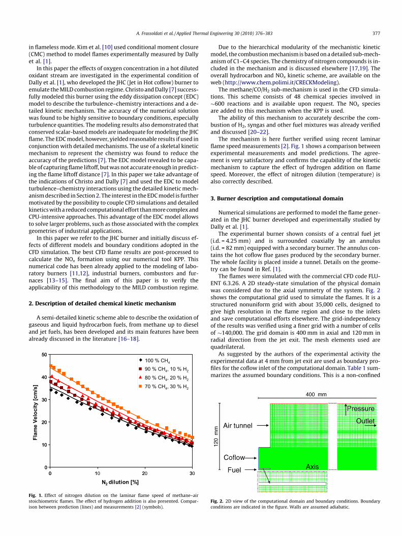
Fig. 1. Effect of nitrogen dilution on the laminar flame speed of methane–airstoichiometric flames. The effect of hydrogen addition is also presented. Compar-ison between prediction (lines) and measurements [2] (symbols).

Due to the hierarchical modularity of the mechanistic kineticmodel, the combustion mechanism is based on a detailed sub-mech-anism of C1–C4 species. The chemistry of nitrogen compounds is in-cluded in the mechanism and is discussed elsewhere [17,19]. Theoverall hydrocarbon and NOx kinetic scheme, are available on theweb (http://www.chem.polimi.it/CRECKModeling).

The methane/CO/H2 sub-mechanism is used in the CFD simula-tions. This scheme consists of 48 chemical species involved in�600 reactions and is available upon request. The NOx speciesare added to this mechanism when the KPP is used.

The ability of this mechanism to accurately describe the com-bustion of H2, syngas and other fuel mixtures was already verifiedand discussed [20–22].

The mechanism is here further verified using recent laminarflame speed measurements [2]. Fig. 1 shows a comparison betweenexperimental measurements and model predictions. The agree-ment is very satisfactory and confirms the capability of the kineticmechanism to capture the effect of hydrogen addition on flamespeed. Moreover, the effect of nitrogen dilution (temperature) isalso correctly described.

3. Burner description and computational domain

Numerical simulations are performed to model the flame gener-ated in the JHC burner developed and experimentally studied byDally et al. [1].

The experimental burner shown consists of a central fuel jet(i.d. = 4.25 mm) and is surrounded coaxially by an annulus(i.d. = 82 mm) equipped with a secondary burner. The annulus con-tains the hot coflow flue gases produced by the secondary burner.The whole facility is placed inside a tunnel. Details on the geome-try can be found in Ref. [1].

The flames were simulated with the commercial CFD code FLU-ENT 6.3.26. A 2D steady-state simulation of the physical domainwas considered due to the axial symmetry of the system. Fig. 2shows the computational grid used to simulate the flames. It is astructured nonuniform grid with about 35,000 cells, designed togive high resolution in the flame region and close to the inletsand save computational efforts elsewhere. The grid-independencyof the results was verified using a finer grid with a number of cellsof �140,000. The grid domain is 400 mm in axial and 120 mm inradial direction from the jet exit. The mesh elements used arequadrilateral.

As suggested by the authors of the experimental activity theexperimental data at 4 mm from jet exit are used as boundary pro-files for the coflow inlet of the computational domain. Table 1 sum-marizes the assumed boundary conditions. This is a non-confined

Fig. 2. 2D view of the computational domain and boundary conditions. Boundaryconditions are indicated in the figure. Walls are assumed adiabatic.

Table 1Boundary conditions.

Central Jet Coflow Tunnel

Temperature (K) 305 1300 294Inlet velocity (m/s) 58.74 3.2 3.3Composition [mass fraction] 0.88 CH4 Measured Profiles [1] 0.232 O2

0.11 H2 0.768 N2

0

0.2

0.4

0.6

0.8

1

0 0.05 0.1 0.15 0.2

Modified k-ε

Axial distance, z [m]

Mix

ture

Frac

tion

RSMStandard k-ε

Exp [7]

0

0.2

0.4

0.6

0.8

1

0 0.05 0.1 0.15 0.2

Modified k-ε

RSMStandard k-ε

Exp [7]

Fig. 4. Axial profiles of mixture fraction along the axis of symmetry for differentturbulence models (9% O2 flame).

378 A. Frassoldati et al. / Applied Thermal Engineering 30 (2010) 376–383

flame, for this reason a pressure outlet condition is used (see Fig. 2)assuming ambient air conditions for the backflow. The simulationswere performed with three different O2 mass fraction profiles inthe coflow. The mean (approximate) O2 mass fractions in coflowprofiles are 3%, 6% and 9%. Fig. 3 shows the relevant effect of thedifferent amount of oxygen in the oxidizer. A flame lift off is visibleand combustion occurs with weaker or higher intensity accordingto the oxygen content in the oxidizer stream.

4. Numerical modeling

The burner was modeled using several turbulence and radiationmodels to simulate the flames. Turbulence was modeled via theRANS approach, using the k–e and the Reynolds Stress Model (RSM).

The Standard k–e model is known for its shortcomings in pre-dicting round jets. In particular, the standard k–e model overpre-dicts the decay rate and the spreading rate of a round jet.Modifications for the parameter Ce1 lead to a value of 1.60 forself-similar round jets [23].

Fig. 4 shows the comparison between experimental measure-ments and model predictions along the axis of symmetry. Mixturefraction is used to describe the mixing between the fuel jet and thesurrounding oxidizer and it is also a good indicator of the jet penetra-tion. The RSM and the modified k–e model perform very well whilethe standard k–e model under predicts the jet penetration. The k–emodel is used in all the simulations in order to avoid the additionalcomputational expense of the Reynolds stress model, and to concen-trate on the study of turbulence–chemistry interactions.

As already observed [7], the numerical solution is highly sensi-tive to the turbulence level at the inlets. In order to reduce thecomputational time and effort, it was decided not to simulate thecomplete (complex) geometry ahead of the coflow inlet, which

Fig. 3. Temperature field [K]: effect of the oxygen content in the oxidizer stream[mass fractions 3%, 6%, 9%].

contains a secondary burner and a perforated plate. For the fuel in-let, the turbulence level proposed in [7] is used. It is important tonotice that the turbulence level at the coflow inlet boundary di-rectly affects the value of the turbulent viscosity, which controlsthe turbulent diffusion. For this reason, the amount of oxygenwhich diffuses form the shroud air towards the flame is signifi-cantly affected by the coflow boundary conditions.

Fig. 5 shows the effect of different values used of the boundarycondition of the turbulent kinetic energy. As expected, the lowerthe value of k is, the lower the diffusion of oxygen from the sur-rounding air to the flame region. Fig. 6 shows the effect of the dif-ferent k values on the O2 radial profiles at two different axiallocations (z = 30 mm and z = 120 mm). The comparison shows thata value of k = 0.4 m2/s2, when used for simulating the flame re-sulted in good agreement with experimental measurements.

Fig. 5. Effect of the boundary condition adopted for the turbulent kinetic energy ofthe coflow stream (3% O2 flame).

0.00

0.05

0.10

0.15

0.20

0.25

0.00 0.02 0.04 0.06

Radial Distance [m]

O2 [

mas

s fr

actio

n]

0.00

0.05

0.10

0.15

0.20

0.25

0.00 0.02 0.04 0.06

Radial Distance [m]

O2 [

mas

s fr

actio

n]

mm021=zmm03=z

3% O2 expk = 0.04 m2/s2

k = 0.40 m2/s2

k = 2.00 m2/s2

0.00

0.05

0.10

0.15

0.20

0.25

O2 [

mas

s fr

actio

n]

0.00

0.05

0.10

0.15

0.20

0.25

O2 [

mas

s fr

actio

n]

mm021=zmm03=z

3% O2 expk = 0.04 m2/s2

k = 0.40 m2/s2

k = 2.00 m2/s2

3% O2 expk = 0.04 m2/s2

k = 0.40 m2/s2

k = 2.00 m2/s2

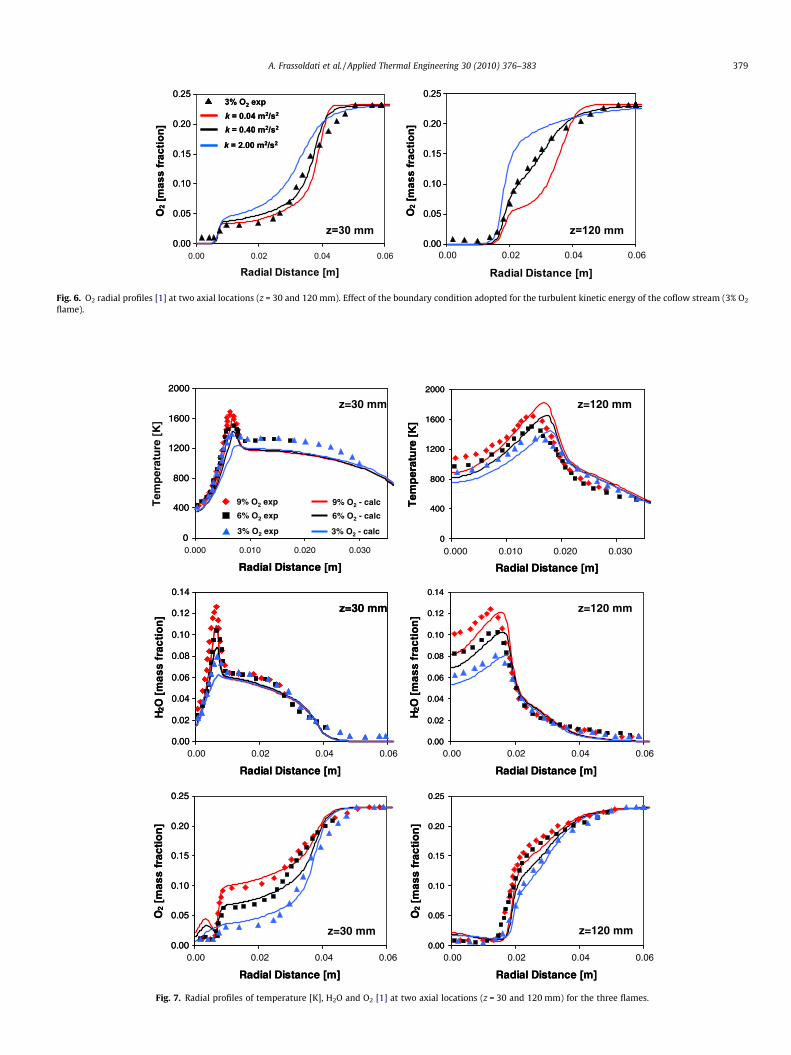
Fig. 6. O2 radial profiles [1] at two axial locations (z = 30 and 120 mm). Effect of the boundary condition adopted for the turbulent kinetic energy of the coflow stream (3% O2

flame).

0

400

800

1200

1600

2000

0.000 0.010 0.020 0.030 0.000 0.010 0.020 0.030

Radial Distance [m]

Tem

per

atu

re [

K]

0

400

800

1200

1600

2000

Radial Distance [m]

Tem

per

atu

re [

K]

mm021=zmm03=z

0.00

0.02

0.04

0.06

0.08

0.10

0.12

0.14

0.00 0.02 0.04 0.06

Radial Distance [m]

H2O

[m

ass

frac

tio

n]

0.00

0.02

0.04

0.06

0.08

0.10

0.12

0.14

0.00 0.02 0.04 0.06

Radial Distance [m]

H2O

[m

ass

frac

tio

n]

mm021=zmm03=z

0.00

0.05

0.10

0.15

0.20

0.25

0.00 0.02 0.04 0.06

Radial Distance [m]

O2

[mas

s fr

acti

on

]

0.00

0.05

0.10

0.15

0.20

0.25

0.00 0.02 0.04 0.06

Radial Distance [m]

O2

[mas

s fr

acti

on

]

z=30 mm z=120 mm

9% O2 exp 9% O2 - calc

6% O2 - calc

3% O2 - calc

6% O2 exp

3% O2 exp0

400

800

1200

1600

2000

Radial Distance [m]

0

400

800

1200

1600

2000

Radial Distance [m]

Tem

per

atu

re [

K]

mm021=zmm03=z

0.00

0.02

0.04

0.06

0.08

0.10

0.12

0.14

Radial Distance [m]

H2O

[m

ass

frac

tio

n]

0.00

0.02

0.04

0.06

0.08

0.10

0.12

0.14

Radial Distance [m]

H2O

[m

ass

frac

tio

n]

mm021=zmm03=z

0.00

0.05

0.10

0.15

0.20

0.25

Radial Distance [m]

O2

[mas

s fr

acti

on

]

0.00

0.05

0.10

0.15

0.20

0.25

Radial Distance [m]

O2

[mas

s fr

acti

on

]

z=30 mm z=120 mm

9% O2 exp 9% O2 - calc

6% O2 - calc

3% O2 - calc

6% O2 exp

3% O2 exp

Fig. 7. Radial profiles of temperature [K], H2O and O2 [1] at two axial locations (z = 30 and 120 mm) for the three flames.

A. Frassoldati et al. / Applied Thermal Engineering 30 (2010) 376–383 379

380 A. Frassoldati et al. / Applied Thermal Engineering 30 (2010) 376–383

We used different radiation models (P1, discrete ordinates (DO)[24] and Sandia model [25]). Although in this particular burnerconfiguration the effect of thermal radiation is not particularly sig-nificant, especially in the first part of the flame, the best resultswere found using the DO model. The WSGGM (weighted sum ofgray gas) model is used to calculate the total emissivity as a func-tion of gas composition and temperature. Different models wereused for the description of the turbulence–chemistry interactions.As already observed by Christo and Dally [7], using detailed chem-ical kinetics, rather than global or skeletal mechanisms improvesthe accuracy significantly. Differential diffusion is always ac-counted for, as it is known to have a strong influence on predic-tions because of the high hydrogen content in the fuel [7]. Acomparison between the modeling and experimental data is pre-sented in Figs. 7 and 8 for the three flames with different oxygenlevels in the hot coflow (9%, 6%, and 3%). Only the results obtainedwith the detailed mechanism presented in Section 2 are discussed.Among the different simulations, in the figures we always refer tothe model results obtained using the modified k–e, the DO radia-tion model and the EDC model for the turbulence–chemistry inter-actions. Details on the EDC model can be found in Refs. [12,26],while examples of its use to model complex situations wherenon-premixed and premixed conditions co-exist are presented byAlbrecht et al. [27] and Tang et al. [28].

The temperature profiles are in good agreement with measure-ments, although the flames lift off is slightly over estimated. Thetemperature peaks at 120 mm are overestimated, especially inthe case of 6% and 9% O2. A possible explanation for this discrep-ancy can be found in the corresponding oxygen radial profiles(Fig. 7). As already discussed, these profiles are affected by the tur-bulence kinetic energy conditions adopted at the coflow boundary.The value of k = 0.4 m2/s2 gives result with a good agreement forthe 3% O2 flame, while in the other cases the diffusion of oxygenis slightly overestimated. The increased availability of oxygen in-

0.000

0.005

0.010

0.015

0.020

0.025

0.00 0.01 0.02 0.03 0.04

0.00 0.01 0.02 0.03 0.04

Radial Distance [m]

CO

[mas

s fr

actio

n] 9% O2 exp 9% O2 - calc6% O2 - calc

3% O2 - calc

6% O2 exp

3% O2 exp

mm03=z

0.0E+00

4.0E-04

8.0E-04

1.2E-03

1.6E-03

Radial Distance [m]

OH

[mas

s fr

actio

n]

mm03=z

0.000

0.005

0.010

0.015

0.020

0.025

9% O2 exp 9% O2 - calc6% O2 - calc

3% O2 - calc

6% O2 exp

3% O2 exp

mm03=z

0.0E+00

4.0E-04

8.0E-04

1.2E-03

1.6E-03

OH

[mas

s fr

actio

n]

mm03=z

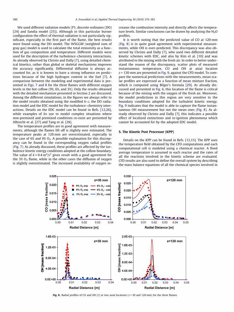
Fig. 8. Radial profiles of CO and OH [1] at two axial lo

creases the combustion intensity and directly affects the tempera-ture levels. Similar conclusions can be drawn by analyzing the H2Oprofiles.

It is worth noting that the predicted value of CO at 120 mm(Fig. 8) is in quite good agreement with experimental measure-ments, while OH is over-predicted. This discrepancy was also ob-served by Christo and Dally [7], who used two different detailedkinetic schemes with EDC, and also by Kim et al. [10] and wasattributed to the mixing with the fresh air. In order to better under-stand the reason of the discrepancy, scatter plots of measuredinstantaneous temperature, CO and OH at axial locationz = 120 mm are presented in Fig. 9, against the CFD model. To com-pare the numerical predictions with the measurements, mean sca-lar profiles are expressed as a function of mean mixture fraction,which is computed using Bilger’s formula [29]. As already dis-cussed and presented in Fig. 6, this location of the flame is criticalbecause of the mixing with the oxygen of the fresh air. Moreover,the model predictions in this region are very sensitive to theboundary conditions adopted for the turbulent kinetic energy.Fig. 9 indicates that the model is able to capture the flame instan-taneous OH measurement but not the mean ones (Fig. 8). As al-ready observed by Christo and Dally [7], this indicates a possibleeffect of localized extinctions and re-ignition phenomena whichcannot be accounted for by the adopted EDC model.

5. The Kinetic Post Processor (KPP)

Details on the KPP can be found in Refs. [12,15]. The KPP usesthe temperature field obtained by the CFD computations and eachcomputational cell is modeled using a chemical reactor. A fixedaverage temperature is assumed in each reactor and the rates ofall the reactions involved in the kinetic scheme are evaluated.CFD results are also used to define the overall system by describingthe mass balance equations of all the chemical species involved in

0.000

0.005

0.010

0.015

0.020

0.025

0.030

0.00 0.01 0.02 0.03 0.04 0.05

0.00 0.01 0.02 0.03 0.04 0.05

Radial Distance [m]

CO

[mas

s fr

actio

n]

mm021=z

0.0E+00

4.0E-04

8.0E-04

1.2E-03

1.6E-03

2.0E-03

Radial Distance [m]

OH

[mas

s fr

actio

n]

mm021=z

0.000

0.005

0.010

0.015

0.020

0.025

0.030

CO

[mas

s fr

actio

n]

mm021=z

0.0E+00

4.0E-04

8.0E-04

1.2E-03

1.6E-03

2.0E-03

mm021=z

cations (z = 30 and 120 mm) for the three flames.

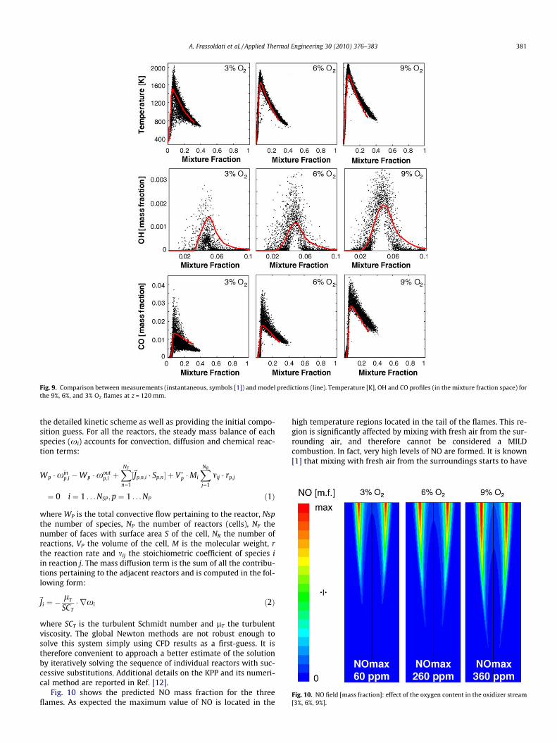
Fig. 9. Comparison between measurements (instantaneous, symbols [1]) and model predictions (line). Temperature [K], OH and CO profiles (in the mixture fraction space) forthe 9%, 6%, and 3% O2 flames at z = 120 mm.

Fig. 10. NO field [mass fraction]: effect of the oxygen content in the oxidizer stream[3%, 6%, 9%].

A. Frassoldati et al. / Applied Thermal Engineering 30 (2010) 376–383 381

the detailed kinetic scheme as well as providing the initial compo-sition guess. For all the reactors, the steady mass balance of eachspecies (xi) accounts for convection, diffusion and chemical reac-tion terms:

Wp �xinp;i �Wp �xout

p;i þXNF

n¼1

½~Jp;n;i � Sp;n� þ V�p �Mi

XNR

j¼1

mij � rp;j

¼ 0 i ¼ 1 . . . NSP;p ¼ 1 . . . NP ð1Þ

where WP is the total convective flow pertaining to the reactor, Nspthe number of species, NP the number of reactors (cells), NF thenumber of faces with surface area S of the cell, NR the number ofreactions, VP the volume of the cell, M is the molecular weight, rthe reaction rate and mij the stoichiometric coefficient of species iin reaction j. The mass diffusion term is the sum of all the contribu-tions pertaining to the adjacent reactors and is computed in the fol-lowing form:

~Ji ¼ �lT

SCT� rxi ð2Þ

where SCT is the turbulent Schmidt number and lT the turbulentviscosity. The global Newton methods are not robust enough tosolve this system simply using CFD results as a first-guess. It istherefore convenient to approach a better estimate of the solutionby iteratively solving the sequence of individual reactors with suc-cessive substitutions. Additional details on the KPP and its numeri-cal method are reported in Ref. [12].

Fig. 10 shows the predicted NO mass fraction for the threeflames. As expected the maximum value of NO is located in the

high temperature regions located in the tail of the flames. This re-gion is significantly affected by mixing with fresh air from the sur-rounding air, and therefore cannot be considered a MILDcombustion. In fact, very high levels of NO are formed. It is known[1] that mixing with fresh air from the surroundings starts to have

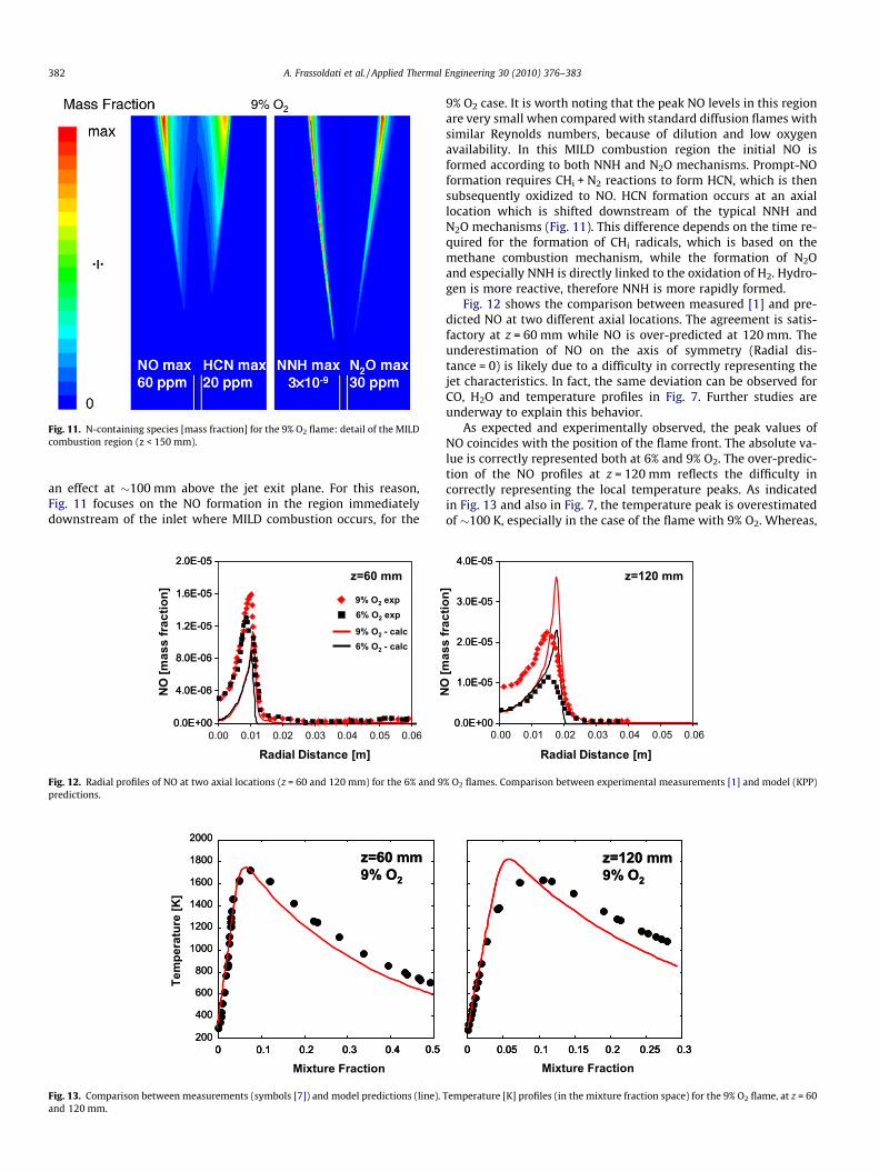
Fig. 11. N-containing species [mass fraction] for the 9% O2 flame: detail of the MILDcombustion region (z < 150 mm).

382 A. Frassoldati et al. / Applied Thermal Engineering 30 (2010) 376–383

an effect at �100 mm above the jet exit plane. For this reason,Fig. 11 focuses on the NO formation in the region immediatelydownstream of the inlet where MILD combustion occurs, for the

0.0E+00

4.0E-06

8.0E-06

1.2E-05

1.6E-05

2.0E-05

0.00 0.01 0.02 0.03 0.04 0.05 0.06

Radial Distance [m]

NO

[mas

s fr

actio

n] 9% O2 exp

9% O2 - calc6% O2 - calc

6% O2 exp

mm06=z

0.0E+00

4.0E-06

8.0E-06

1.2E-05

1.6E-05

2.0E-05

9% O2 exp

9% O2 - calc6% O2 - calc

6% O2 exp

mm06=z

Fig. 12. Radial profiles of NO at two axial locations (z = 60 and 120 mm) for the 6% and 9predictions.

0 0.1 0.2 0.3 0.4 0.5

Mixture Fraction

400

600

800

1000

1200

1400

1600

1800

2000

200

Tem

pera

ture

[K]

z=60 mm9% O2

0 0.1 0.2 0.3 0.4 0.50 0.1 0.2 0.3 0.4 0.5

400

600

800

1000

1200

1400

1600

1800

2000

200

z=60 mm9% O2

Fig. 13. Comparison between measurements (symbols [7]) and model predictions (line).and 120 mm.

9% O2 case. It is worth noting that the peak NO levels in this regionare very small when compared with standard diffusion flames withsimilar Reynolds numbers, because of dilution and low oxygenavailability. In this MILD combustion region the initial NO isformed according to both NNH and N2O mechanisms. Prompt-NOformation requires CHi + N2 reactions to form HCN, which is thensubsequently oxidized to NO. HCN formation occurs at an axiallocation which is shifted downstream of the typical NNH andN2O mechanisms (Fig. 11). This difference depends on the time re-quired for the formation of CHi radicals, which is based on themethane combustion mechanism, while the formation of N2Oand especially NNH is directly linked to the oxidation of H2. Hydro-gen is more reactive, therefore NNH is more rapidly formed.

Fig. 12 shows the comparison between measured [1] and pre-dicted NO at two different axial locations. The agreement is satis-factory at z = 60 mm while NO is over-predicted at 120 mm. Theunderestimation of NO on the axis of symmetry (Radial dis-tance = 0) is likely due to a difficulty in correctly representing thejet characteristics. In fact, the same deviation can be observed forCO, H2O and temperature profiles in Fig. 7. Further studies areunderway to explain this behavior.

As expected and experimentally observed, the peak values ofNO coincides with the position of the flame front. The absolute va-lue is correctly represented both at 6% and 9% O2. The over-predic-tion of the NO profiles at z = 120 mm reflects the difficulty incorrectly representing the local temperature peaks. As indicatedin Fig. 13 and also in Fig. 7, the temperature peak is overestimatedof �100 K, especially in the case of the flame with 9% O2. Whereas,

0.00 0.01 0.02 0.03 0.04 0.05 0.060.0E+00

1.0E-05

2.0E-05

3.0E-05

4.0E-05

Radial Distance [m]

NO

[mas

s fr

actio

n]

mm021=z

0.0E+00

1.0E-05

2.0E-05

3.0E-05

4.0E-05mm021=z

% O2 flames. Comparison between experimental measurements [1] and model (KPP)

0 0.05 0.1 0.15 0.2 0.25 0.3

Mixture Fraction

z=120 mm9% O2

0 0.05 0.1 0.15 0.2 0.25 0.30 0.05 0.1 0.15 0.2 0.25 0.3

z=120 mm9% O2

Temperature [K] profiles (in the mixture fraction space) for the 9% O2 flame, at z = 60

A. Frassoldati et al. / Applied Thermal Engineering 30 (2010) 376–383 383

Fig. 13 indicates that the temperature peak at z = 60 mm is in goodagreement with experimental measurements, which resulted ingood prediction of the NOx profile although it is slightly underesti-mated. This observation indicates that a progress in the KPP simu-lations is possible only on the basis of an improved CFD simulation.

6. Conclusions

A detailed CFD study of a CH4/H2 MILD combustion burner (JHC)has been presented using different turbulence and radiation mod-els. A detailed kinetic mechanism able to describe the combustionof light hydrocarbons is used in the CFD simulations using the EDCapproach to model turbulent combustion. This scheme is here fur-ther validated using recent experimental data on the effect nitro-gen dilution on the flame velocity of CH4 and CH4/H2 mixtures.

Due to the mixing with the surrounding fresh air, the accuracyof the numerical solution is found to be highly sensitive to bound-ary conditions, especially turbulence quantities. The modified k–emodel succeeded in simulating the fuel jet fluid dynamics flamestructure.

CFD results were validated using experimental measurementsand then post-processed using a detailed Kinetic Post Processor(KPP). The computed results were validated in terms of NO forma-tion and the overall agreement with experimental measurementsis satisfactory.

The discrepancies between measured and predicted NO profilescan be attributed to the overestimation of the temperature field ataxial distances larger than �100 mm. In this region the mixingwith surrounding air is known to play a significant role. An impor-tant goal of the future activity will be to better describe the condi-tions at the boundaries to improve the CFD simulation in thisregion. Nevertheless, the results are encouraging and the modelwill be applied for the design of new advanced combustors. Ofcourse, the reliability of KPP predictions is strongly dependent onthe accuracy of the CFD simulation.

Acknowledgements

The authors gratefully acknowledge the financial support ofRIELLO SpA – Burners Division and MSE-CNR for the support insidethe project ‘‘Accordo di Programma MSE-CNR per la Ricerca di Sis-tema elettrico Nazionale”.

References

[1] B.B. Dally, A.N. Karpetis, R.S. Barlow, Proc. Combust. Inst. 29 (1) (2002) 1147–1154.

[2] T. Tatouh, F. Halter, C. Mouna-Rousselle, The effect of hydrogen enrichment onCH4 – air combustion in strong dilution, XXXI Meeting on Combustion, Torino,2008. June 17–20.

[3] J.A. Wünning, J.G. Wünning, Prog. Energy Combust. Sci. 23 (12) (1997) 81–94.[4] R. Weber, A.L. Verlaan, S. Orsino, N. Lallemant, J. Inst. Energy 72 (1999) 77–83.

[5] M. Katsuki, T. Hasegawa, Science and technology of combustion in highlypreheated air, Proc. Combust. Inst. 27 (1998) 3135.

[6] M. De Joannon, A. Saponaro, A. Cavaliere, Zero-dimensional analysis of dilutedoxidation of methane in rich conditions, Proc. Combust. Inst. 28 (2) (2000)1639–1645.

[7] F.C. Christo, B.B. Dally, Modeling turbulent reacting jets issuing into a hot anddiluted coflow, Combust. Flame 142 (1–2) (2005) 117–129.

[8] P.J. Coelho, N. Peters, Numerical simulation of a mild combustion burner,Combust. Flame 124 (3) (2001) 503–518.

[9] .M. Mancini, R. Weber, U. Bollettini, Predicting NOx emissions of a burneroperated in flameless oxidation mode, Proc. Comb. Inst. 29 (1) (2002) 1155–1162.

[10] S.H. Kim, K.Y. Huh, B. Dally, CMC modeling of turbulent nonpremixedcombustion in diluted hot coflow, Proc. Comb. Inst. 30 (1) (2004) 751–757.

[11] A. Frassoldati, S. Frigerio, E. Colombo, F. Inzoli, T. Faravelli, Determination ofNOx emissions from strong swirling confined flames with an integrated CFD-based procedure, Chem. Eng. Sci. 60 (2005) 2851–2869.

[12] A. Cuoci, A. Frassoldati, G. Buzzi Ferraris, T. Faravelli, E. Ranzi, Ignition, Fluiddynamics and kinetics aspects of syngas combustion, Int. J. Hydrogen Energy32 (2007) 3486–3500.

[13] Barendregt, I. Risseeuw, F. Waterreus, A. Frassoldati, G. Buzzi Ferraris, T.Faravelli, E. Ranzi, X.J. Li, A.R. Patel, Combustion modeling of ethylene furnacesapplying ultra low NOx LSVTM burners, In: AIChE Spring Annual Meeting, 2006.

[14] A. Frassoldati, A. Cuoci, T. Faravelli, E. Ranzi, S. Colantuoni, P. Di Martino, G.Cinque, Experimental and modeling study of a low NOx combustor for aero-engine turbofan, Combust. Sci. Tech. 181 (2009) 1–13.

[15] A. Frassoldati, A. Cuoci, T. Faravelli, E. Ranzi, D. Astesiano, M. Valenza, P.Sharma, Experimental and modelling study of low-NOx industrial burners,Metall. Plant Technol. Int. 31 (6) (2008) 44–46.

[16] E. Ranzi, A. Sogaro, P. Gaffur, G. Pennati, T. Faravelli, Wide range modelingstudy of methane oxidation, Combust. Sci. Tech. 96 (4–6) (1994) 279–325.

[17] T. Faravelli, A. Frassoldati, E. Ranzi, Kinetic modeling of mutual interactions inNO-hydrocarbon low temperature oxidation, Combust. Flame 132 (1–2)(2003) 188–207.

[18] E. Ranzi, A. Frassoldati, S. Granata, T. Faravelli, Wide-range kinetic modelingstudy of the pyrolysis, partial oxidation, and combustion of heavy n-alkanes,Ind. Eng. Chem. Res. 44 (14) (2005) 5170–5183.

[19] A. Frassoldati, T. Faravelli, E. Ranzi, Kinetic modeling of mutual interactions inNO-hydrocarbon high temperature oxidation, Combust. Flame 135 (2003) 97–112.

[20] A. Frassoldati, T. Faravelli, E. Ranzi, A wide range modelling study of NOx

formation and nitrogen chemistry in hydrogen combustion, Int. J. HydrogenEnergy 31 (15) (2005) 2310–2328.

[21] A. Frassoldati, T. Faravelli, E. Ranzi, Ignition, combustion and flame structure ofcarbon monoxide/hydrogen mixtures. Note 1: detailed kinetic modeling ofsyngas combustion also in presence of nitrogen compounds, Int. J. HydrogenEnergy 32 (2007) 3471–3485.

[22] T. Shimizu, F.A. Williams, A. Frassoldati, Concentrations of nitric oxide inlaminar counterflow methane/air diffusion flames, J. Propul. Power 21 (6)(2005) 1019–1028. November–December.

[23] B.B. Dally, D.F. Fletcher, A.R. Masri, Combust. Theor. Model. 2 (1998) 193.[24] FLUENT 6.3.26, User’s Guide.[25] R.S. Barlow, A.N. Karpetis, J.H. Frank, J.-Y. Chen, Combust. Flame 127 (2001)

2102–2118.[26] B.F. Magnussen, On the structure of turbulence and a generalized Eddy

dissipation concept for chemical reactions in turbulent flows, 19th AIAAaerospace science meeting, St. Louis, Missouri, 1981.

[27] B.A. Albrecht, S. Zahirovic, R.J.M. Bastiaans, J.A. van Oijen, L.P.H. de Goey, Apremixed flamelet-PDF model for biomass combustion in a grate furnace,Energy Fuels 22 (2008) 1570–1580.

[28] Q. Tang, M. Denison, B. Adams, D. Brown, Towards comprehensivecomputational fluid dynamics modeling of pyrolysis furnaces with nextgeneration low-NOx burners using finite-rate chemistry, Proc. Comb. Inst. 32(2009) 2649–2657.

[29] R.W. Bilger, Combust. Flame 80 (1990) 135–149.