A two-factor model of the German term structure of interest rates

E U R O P E A N C E N T R A L B A N K

WO R K I N G PA P E R S E R I E S

WORKING PAPER NO. 46

A TWO-FACTOR MODEL OFTHE GERMAN TERM

STRUCTURE OF INTERESTRATES

BY NUNO CASSOLAAND JORGE BARROS LUÍS

March 2001

E U R O P E A N C E N T R A L B A N K

WO R K I N G PA P E R S E R I E S

* Previous versions of this paper were presented at the ESCB Workshop on Yield Curve Modelling, Frankfurt am Main, 30 March 1999, the European Economics and Financial CentreConference, Maribor, 30 June 1999, the University of York, 4 November 1999, Universidade Católica Portuguesa, Lisbon, 14 February 2000, Banco de Portugal, Lisbon, 17 February2000, the CEMAPRE Conference, Lisbon, 6 June 2000, and the Money, Macro and Finance Research Group 2000 Conference, London, 6 September 2000.The authors are gratefulto Mike Wickens, Peter N. Smith, Menelaos Karanasos, Jerome Henry and João Pedro Nunes for helpful discussions and suggestions, to Ken Singleton and Karim Abadir for helpfulinsights on the estimation procedure and to Fátima Silva for research assistance. The second author also acknowledges the support of the Lisbon Stock Exchange. The usualdisclaimer applies.

** European Central Bank.*** University of York and Banif Investimento.

WORKING PAPER NO. 46

A TWO-FACTOR MODEL OFTHE GERMAN TERM

STRUCTURE OF INTERESTRATES*

BY NUNO CASSOLA**

AND JORGE BARROS LUÍS***

March 2001

© European Central Bank, 2001

Address Kaiserstrasse 29

D-60311 Frankfurt am Main

Germany

Postal address Postfach 16 03 19

D-60066 Frankfurt am Main

Germany

Telephone +49 69 1344 0

Internet http://www.ecb.int

Fax +49 69 1344 6000

Telex 411 144 ecb d

All rights reserved.

Reproduction for educational and non-commercial purposes is permitted provided that the source is acknowledged.

The views expressed in this paper are those of the authors and do not necessarily reflect those of the European Central Bank.

ISSN 1561-0810

3ECB Working Paper No 46 March 2001

Contents

Abstract 5

1 Introduction 7

2 Background issues on asset pricing 10

3 Duffie-Kan affine models of the term structure 12

4 Gaussian affine models 17

5 A forward rate test of the expectations theory 21

6 Identification 23

7 Econometric methodology 26

8 Data and estimation results 27

9 Conclusions 32

Appendix The Kalman Filter 33

References 40

Tables 45

Figures 48

European Central Bank Working Paper Series 60

ECB Working Paper No 46 March 20014

5

In this paper we show that a two-factor constant volatility model providesan adequate description of the dynamics and shape of the German termstructure of interest rates from 1972 up to 1998. The model also providesreasonable estimates of the volatility and term premium curves. Followingthe conjecture that the two factors driving the German term structure ofinterest rates represent the - real interest rate and the expectedinflation rate, the identification of one factor with expected inflation isdiscussed. Our estimates are obtained using a Kalman filter and amaximum likelihood procedure including in the measurement equationboth the yields and their volatilities.

E43, G12.

expectations hypothesis; term premiums; pricing kernels; affine model


7

The identification of the factors that determine the time-series and cross section

behaviour of the term structure of interest rates is a recurrent topic in the finance

literature. Its is a controversial subject that has several empirical and practical

implications, namely for assessing the impact of economic policy measures or for

hedging purposes (see, for instance, Fleming and Remolona (1998) and Bliss

(1997)).

One-factor models were the first step in modelling the term structure of

interest rates. These models are grounded on the estimation of bond yields as

functions of the short-term interest rate. Vasicek (1977) and Cox . (1985) (CIR

hereafter) are the seminal papers within this literature. However, one factor

models do not overcome the discrepancy between the theoretical mean yield

curve implied by the time-series properties of bond yields and the observed

curves that are substantially more concave than implied by the theory (see, for

instance, Backus (1998)).

One answer to this question has been provided by multifactor affine models,

that consider bond yields as functions of several macroeconomic and financial

variables, observable or latent. Affine models are easier to estimate than binomial

models,1 given that the parameters are linear in both the maturity of the assets

and the number of factors.2

Most papers have focused on the U.S. term structure. The pronounced hump-

shape of the US yield curve and the empirical work pioneered by Litterman and

Scheinkman (1991) have led to the conclusion that three factors are required to

explain the movements of the whole term structure of interest rates. These factors

1 In these models, the state variables can go up or down in any unit of time and a probability isattached to each change (see, e.g., Backus . (1998, pp. 15-16)).


8

are usually identified as the level, the slope and the curvature of the term

structure. Most studies have concluded that the level is the most important factor

in explaining interest rate variation over time.

Moreover, given the apparent stochastic properties of the volatility of interest

rates, Gaussian or constant volatility models are often rejected. Therefore, several

papers have used 3-factor models with stochastic volatility in order to fit the

term structure of interest rates (see, for instance, Balduzzi (1996) and Gong

and Remolona (1997 a)).

However, stochastic volatility models pose admissibility problems, as the

factors determining the volatility of interest rates enter “square rooted” and thus

must be positive.3 Additionally, the parameters of a three-factor model with

stochastic volatility are very difficult to estimate. In fact, frequently small

deviations of the parameters from the estimated values generate widely different

and implausible term structures. Furthermore, some term structures may have

properties identifiable with less complex models. For instance, according to

Buhler (1999), principal component analysis reveals that two factors explain

more than 95 percent of the variation in the German term structure of interest

rates consistently from 1970 up to 1999.

To motivate our work we start by performing forward rate regressions

following Backus (1997), in order to assess the adequacy of Gaussian models

to estimate the German term structure of interest rates. These models overcome

the empirical problems posed by stochastic volatility models and are capable of

reproducing a wide variety of shapes of the yield curve, though they face some

2 See Campbell (1997, chapter 11) or Backus . (1998) for graduate textbook presentationsof affine models.3 For a continuous-time presentation and the discussion of admissibility and classificationconditions of the models see Dai and Singleton (1998).


9

shortcomings regarding the limiting properties of the instantaneous forward

rate.4

The model is derived in discrete-time: It matches the frequency of the data,

allows the identification of the factors with observable macro-economic variables

and avoids the problem of estimating continuous-time model with discrete-time

data (see, for example, Aït-Sahalia (1996)).

As the data seems supportive of the constant volatility assumption, we

estimate a two-latent factor Gaussian model. The specification of the model

implies that the short-term interest rate is the sum of a constant with the two

latent factors. This is consistent with the idea that nominal interest rates can be

(approximately) decomposed into two components: the expected rate of inflation

and the expected real interest rate (Fisher hypothesis) or, in the C-CAPM model,

the expected growth rate of consumption.

We use the Kalman Filter to uncover the latent factors and a maximum

likelihood procedure to estimate the time-constant parameters, following the

pioneering work by Chen and Scott (1993a and 1993b).

The two-factor model fits quite well the yield and the volatility curve,

providing reasonable estimates for the one-period forward and term premium

curves. It also provides a good fit of the time series of bond yields.

As Backus (1997) mention, the major outstanding issue is the economic

interpretation of the interest rate behaviour approximated with affine models in

terms of its monetary and real economic factors.5

4 See, e.g., Campbell . (1997), pp. 433, on the limitations of a one-factor homoskedastic model.5 This is also the major theoretical drawback in arbitrage pricing theory (APT) developed by Ross(1976).


10

In line with Zin (1997), our conjecture is that one of the two factors driving the

German term structure of interest rates is related to expected inflation. Thus after

discussing the pros and cons of alternative ways of identifying one factor with

the inflation rate process, we present some econometric evidence on the leading

indicator properties of the second factor for inflation developments in Germany.

The remainder of paper is structured as follows. In the next section some

background on asset pricing is presented. In the third section the theoretical

framework of Duffie and Kan (1996) (DK hereafter) affine models is explained. In

the fourth section a test of the expectations theory is developed that will be used

to empirically motivate the Gaussian model. In the fifth section the Gaussian

model to be estimated is fully specified. In the sixth section we discuss

alternative ways of identifying the factors in the model. The econometric

methodology is presented in the seventh section. Section eighth includes the

presentation of the data and the results of the estimation. The main conclusions

are stated at the end.

! "#$ %$

The main result from modern asset pricing theory states that in an arbitrage-free

environment there exists a positive stochastic discount factor (henceforth sdf,

denoted by W) that gives the price at date of any traded financial asset

providing nominal cash-flows (W) as its discounted future pay-off: 6

6 Within the consumption-based CAPM framework, the pricing kernel corresponds to theintertemporal marginal rate of substitution in consumption, deflated by the inflation rate (see,Campbell . (1997) for a detailed presentation). The analysis is usually conducted on a nominalbasis, following (1), as financial assets providing real cash-flows are scarce. The best knownexamples are the inflation-indexed Government bonds that exist only in a few countries. The UKand the US inflation-indexed Government bonds are the most prominent and their informationcontent has been studied in several papers (see, for instance, Deacon and Derry (1994), Gong andRemolona (1997b) and Remolona (1998)).


11

W W W W

= + +1 1 or1 11

+

+

W

W

W

W

(1)

W is also known as the pricing kernel, given that it is the determining variable

of W. In fact, solving forward the basic pricing equation (1), a model of asset

pricing requires the specification of a stochastic process for the pricing kernel:

W W W W Q

= + +1 ... (2)

Denoting the one-period nominal gross returns W W+1 by 1 1+ +W , and

given that ( ) ( ) [ ] [ ]1 1 1 1 1 11 1 ,W W W W W W W W W W

+ + + + + ++ = + + we get from (1):

W W

W W

W W W1

111

11 1

+

+

+ +, (3)

Therefore a risk-free asset, with gross return equal to 1 1+ +WI , that has a

future pay-off known with complete certainty verifies:

11

11

+ =++

W

I

W W

(4)

Thus, the excess return of any asset over a risk-free asset, measured as the

difference between (3) and (4) is:

W W W WI

WI

W W W + + + + +1 1 1 1 11 , (5)

Equation (5) illustrates a basic result in finance theory: the excess return of any

asset over the risk-free asset depends on the covariance of its rate of return with

the stochastic discount factor. Thus, an asset whose pay-off has a negative

correlation with the stochastic discount factor pays a risk premium.


12

Within the C-CAPM framework the sdf is equal to the marginal utility of

consumption. When consumption growth is high the marginal utility of

consumption is low. Therefore if returns are negatively correlated with the sdf,

high returns are associated with high consumption states of nature. A risk

premium must be paid for investors to hold such an asset because it fails to

provide wealth when it is more valuable for the investor.

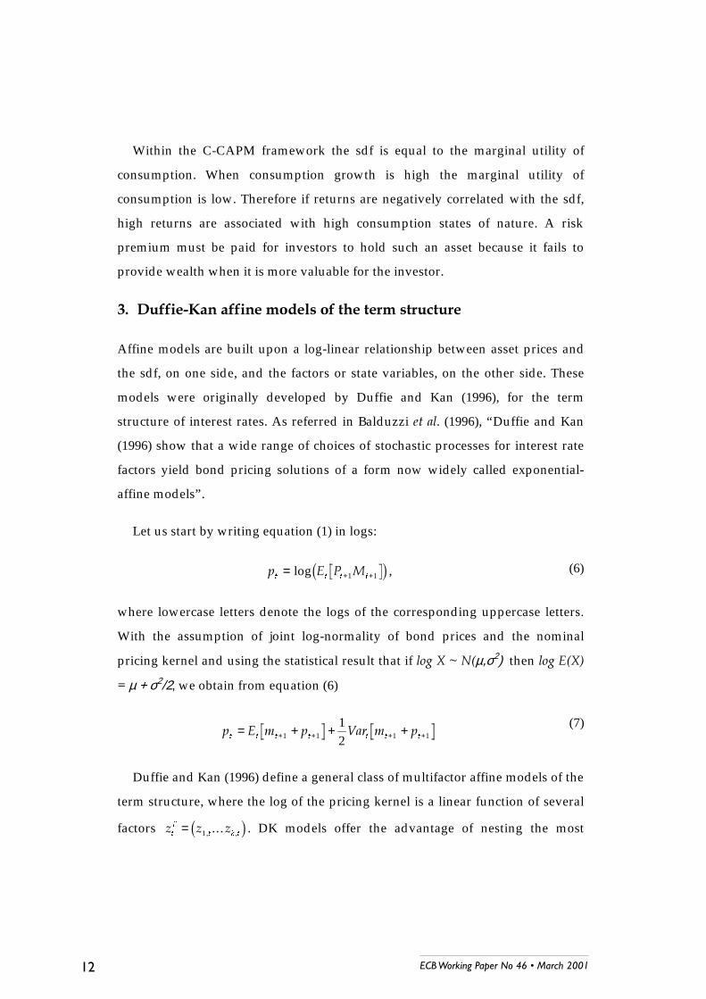
Affine models are built upon a log-linear relationship between asset prices and

the sdf, on one side, and the factors or state variables, on the other side. These

models were originally developed by Duffie and Kan (1996), for the term

structure of interest rates. As referred in Balduzzi . (1996), “Duffie and Kan

(1996) show that a wide range of choices of stochastic processes for interest rate

factors yield bond pricing solutions of a form now widely called exponential-

affine models”.

Let us start by writing equation (1) in logs:

W W W W

= + +log 1 1 , (6)

where lowercase letters denote the logs of the corresponding uppercase letters.

With the assumption of joint log-normality of bond prices and the nominal

pricing kernel and using the statistical result that if µ,σ2) then

µ + σ2/2, we obtain from equation (6)

W W W W W W W

= + + ++ + + +1 1 1 1

12

(7)

Duffie and Kan (1996) define a general class of multifactor affine models of the

term structure, where the log of the pricing kernel is a linear function of several

factors W

7

W N W= 1, ,... . DK models offer the advantage of nesting the most


13

important term structure models, from Vasicek (1977) and CIR one-factor models

to three-factor models like the one presented in Gong and Remolona (1997a). An

additional feature of these models is that they allow the estimation of the term

structure simultaneously on a cross-section and a time-series basis. Furthermore

they provide a way of computing and estimating simple closed-form expressions

for the spot, forward, volatility and term premium curves.

Expressed in discrete time, the discount factors in DK models are specified as:7

− = + ++ + W

7

W

7

W W11 2

1ξ γ λ ε / , (8)

where W is the variance-covariance matrix of the random shocks to the sdf

and is defined as a diagonal matrix with elements L W L L

7

W = +α β . Under

certain conditions, the volatility functions L W are positive;8 βL has nonnegative

elements and εW are the independent shocks normally distributed as ε

W ~ ,0 .

Following (5), the parameters in λ7 are the market prices of risks, as they govern

the covariance between the stochastic discount factor and the latent factors of the

yield curve. Thus, the higher these parameters are, the higher is the covariance

between the discount factor and the asset return and the lower is its expected

rate of return or the less risky the asset is (when the covariance is negative).

The -dimensional vector of factors Wis defined as follows:

W W W W+ += − + +1

1 21Φ Φ θ ε/ , (9)

where Φ has positive diagonal elements which ensure that the factors are

stationary and θ is the long-run mean of the factors. Asset prices are also log-

linear functions of the factors. Adding a second subscript in order to identify the

term to maturity (denoted by ), bond prices are given as follows:

7 See, e.g., Backus (1998).


14

− = + Q W Q Q

7

W, , (10)

where Q is a parameter and Q a vector of parameters to be estimated. The

parameters in Q are commonly known as the factor loadings, given that their

values measure the impact of a one-standard deviation shock to the factors on

the log of asset prices.

In term structure models, the identification of the parameters is easier,

considering the restrictions imposed by the maturing bond price. In fact, when

the term structure is modelled using zero-coupon bonds paying one monetary

unit, the log of the price of a maturing bond must be zero. Consequently, from

(10), the common normalisation 0 = 0 = 0 results. The following recursive

restrictions between the parameters are obtained computing the moments in

equation (7), using equations (8) and (10), equating the independent terms and

the terms in W in equation (9) respectively to Q and Q in (10) and assuming

0,W=0:

Q Q Q

7

L L Q L

L

N

= + + − − +− − −=∑1 1 1

2

1

12

ξ θ λ αΦ , ,(11)

Q

7 7

Q

7

L L Q L

7

L

N

= + − +− −=∑γ λ β1 1

2

1

12

Φ , ,(12)

Our empirical analysis is based on interest rates of nominal zero-coupon

bonds. Continuously compounded yields to maturity of discount bonds or spot

rates ( Q,W) can be easily computed from bond prices as:

Q W

Q W

,,= −

(13)

Consequently, from (10) and (13), the yield curve is defined as:

8 See Backus (1998).


15

Q W Q Q

7

W, = +1 (14)

Using equations (11), (12) and (14), the short-term or one-period interest rate

is:

W L L

L

N

7

L L

7

L

N

W12

1

2

1

12

12, = − + −

= =

∑ ∑ξ λ α γ λ β(15)

Correspondingly, the expected value of the short rate is:

W W Q W L L

L

N

7

L L

7

L

N

W Q

L L

L

N

7

L L

7

L

N

W W Q

L L

L

N

7

L L

7

L

N

Q Q

W

12

1

2

1

2

1

2

1

2

1

2

1

1

2

1

2

1

2

1

2

1

2

1

2

, += =

+

= =

+

= =

ξ λ α γ λ β

ξ λ α γ λ β

ξ λ α γ λ β θ

,

(16)

The volatility curve of the yields is derived from the variance-covariance

matrix in the specification of the factors. From equations (9) and (14), the

volatility curve is given by:

W Q W Q

7

W Q, + =1 2

1 .(17)

The instantaneous or one-period forward rate is the log of the inverse of the

gross return:

Q W Q W Q W, , ,= − +1 . (18)

According to the definition in (18), the price equation in (10) and the recursive

restrictions in (11) and (12), the one-period forward curve is:


16

!

Q W Q Q

7

W Q Q

7

W

Q

7

L L Q L

L

N

7

Q

7

L L Q L

7

L

N

W

,

, ,

= + − +

= + − − + + + − − +

+ +

= =∑ ∑

1 1

2

1

2

1

12

12

ξ θ λ α γ λ βΦ Φ

(19)

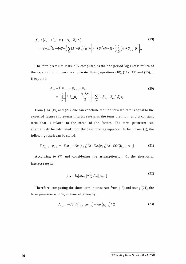
The term premium is usually computed as the one-period log excess return of

the -period bond over the short-rate. Using equations (10), (11), (12) and (15), it

is equal to:

Q W W Q W Q W W

L L Q L

L Q L

L

N

L L Q L Q

L

N

L

7

W

, , , ,

,,

, ,

+ +

= =

1 1 1

2

1

2

12λ α

αλ β

(20)

From (16), (19) and (20), one can conclude that the forward rate is equal to the

expected future short-term interest rate plus the term premium and a constant

term that is related to the mean of the factors. The term premium can

alternatively be calculated from the basic pricing equation. In fact, from (1), the

following result can be stated:

W Q W Q W W W W Q W W W W Q W W, , , ,/ / ,

+ + + + + + + 1 1 1 1 1 1 12 2 (21)

According to (7) and considering the assumption W0 0= , the short-term

interest rate is:

W W W W W1 1 1

12, = ++ +

(22)

Therefore, computing the short-term interest rate from (13) and using (21), the

term premium will be, in general, given by:

Q W W Q W W W Q W

" , , ,, / + + +1 1 1 2 (23)


17

Equation (23) tells us that the term premium is determined by the covariance

of the asset’s rate of return with the stochastic discount factor and a Jensen’s

inequality term resulting from the fact that the risk-premium is computed as the

log-excess return. Thus, in line with equation (5), the lower the covariance, the

higher the term premium is.

As from (10) Q W Q W Q W Q Q

7

W Q Q

7

W, , ,+ − + + + += − = − − + +1 1 1 1 1 1 , the covariance in

(23) is − + + Q

7

W W W1 1, and the conditional variances of the factors correspond

to Q

7

W W Q+1 . Consequently, equation (23) is equivalent to:

Q W Q

7

W W Q

7

W W Q , , /

+ + +1 1 1 2 (24)

According to (8) and (9), the term premium may be written from (24) as:

Q W

7

W Q

Q

7

W Q

, λ 2

(25)

Given that W was previously defined as a diagonal matrix with elements

L W L L

7

W = +α β , equation (25) corresponds to (20). The first component in (25) is

a pure risk premium, where λ is the price associated with the quantity of risk

W Q . The parameters in λ determine the signal of the term premium. The

second component is a Jensen inequality term.

The model we estimate belongs to the class of Gaussian or constant volatility

models. It is a generalisation of the Vasicek (1977) one-factor model and a

particular case of the DK model, implying that some form of the expectations

theory holds. As it will be seen, this model seems to be adequate to fit the

German term structure, as the expectations theory is valid to a close

approximation in this case.


18

Following equation (8), the sdf in a two-factor Gaussian model is written as:9

− = + + +

+ +

=∑

W

L

L LW L L L W

L

N

1

22

11 2

δ λ σ λ σ ε , .(26)

with = 2. The factors are assumed to follow a first-order autoregressive order,

with zero mean:10

L W L LW L L W, ,+ += +1 1ϕ σ ε , with = 1 2, . (27)

Within the DK framework, these models are characterised by:

θϕ ϕ

α σβ

ξ δ λ σ

γ

L

L L

L

L

L

L

N

L

#

=

=

==

= +

==∑

0

0

21

1 2

2

22

1

Φ ,

.

(28)

The recursive restrictions are:

Q Q L L L L L Q L

L

N

= + + − +− −=∑1

2 21

2

1

12

δ λ σ λ σ σ, , (29)

L Q L Q L, ,= + −1 1ϕ . (30)

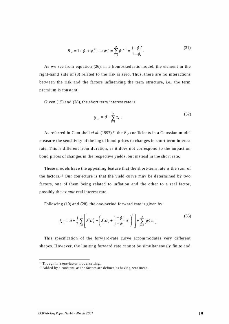
Notice that, according to the auto-regressive pattern evidenced in equation

(30), each L Q, corresponds to the sum of the -terms of a geometric progression:

9 As it will be seen later, this specification was chosen in order to write the short-term interest rateas the sum of a constant (δ) with the factors.10 This corresponds to considering the differences between the “true” factors and their means.


19

L Q L L L

Q

L

Q

L

Q

L

Q

L

, ...

-

=

11

12 1

1

ϕ ϕ ϕ ϕ ϕϕ

.(31)

As we see from equation (26), in a homoskedastic model, the element in the

right-hand side of (8) related to the risk is zero. Thus, there are no interactions

between the risk and the factors influencing the term structure, i.e., the term

premium is constant.

Given (15) and (28), the short term interest rate is:

W LW

L

N

11

, = +=∑δ .

(32)

As referred in Campbell . (1997),11 the L,Q coefficients in a Gaussian model

measure the sensitivity of the log of bond prices to changes in short-term interest

rate. This is different from duration, as it does not correspond to the impact on

bond prices of changes in the respective yields, but instead in the short rate.

These models have the appealing feature that the short-term rate is the sum of

the factors.12 Our conjecture is that the yield curve may be determined by two

factors, one of them being related to inflation and the other to a real factor,

possibly the $real interest rate.

Following (19) and (28), the one-period forward rate is given by:

! Q W L L L L

L

Q

L

L

L

N

L

Q

LW

L

N

, = + − +−−

+

= =∑ ∑δ λ σ λ σ ϕ

ϕσ ϕ1

211

2 2

2

1 1

(33)

This specification of the forward-rate curve accommodates very different

shapes. However, the limiting forward rate cannot be simultaneously finite and

11 Though in a one-factor model setting.12 Added by a constant, as the factors are defined as having zero mean.


20

time-varying. In fact, if ϕL<1,the limiting value will not depend on the factors,

corresponding to the following expression:13

lim ,!Q W

Q

L L

L

L

LL

N

→∞ =

= + −−

−−

∑δ λ σ

ϕσ

ϕ

2 2

21 1 2 1

(34)

From (17) and (28), the volatility curve is:

W Q W L Q L

L

N

, ,+=

= ∑1 22 2

1

1 σ , (35)

Notice that as the factors have constant volatility, given by W L W L, + =1

2 σ , the

volatility of the yields does not depend on the level of the factors.

From (20) and (28), the term premium in these models will be:

ΛQ W W Q W Q W W

L L L L

L

Q

L

L

L

N

L L L Q

L Q L

L

N

, , , ,

,,

= − − =

= − +−−

=

= − −

+ +

=

=

∑

∑

1 1 1

2 2

2

1

22 2

1

1

2

1

1

2

λ σ λ σ ϕϕ

σ

λ σσ

,

(36)

According to (33) and (36), the one-period forward rate in these Gaussian

models corresponds to the sum of the term premium with a constant and with

the factors weighted by the autoregressive parameters of the factors. Once again,

the limiting case is worth noting. When ϕL<1, the limiting value of the risk

13 If ϕ

L= 1 interest rates are non-stationary. In that case, the limiting value of the instantaneous

forward is time-varying but assumes infinite values. Effectively, according to (31), 11

−−

=ϕϕ

L

Q

L

in this case. Thus, the expression for the instantaneous forward will be given by

! Q W L L L

L

N

LW

L

N

, = + − −

+

= =∑ ∑δ λ σ σ2 2 2

1 1

12

. Accordingly, even if λL <0, the forward rate curve

may start by increasing, but at the longer end it will decrease infinitely. Obviously, if λL >0, theforward rate curve will decrease monotonously.


21

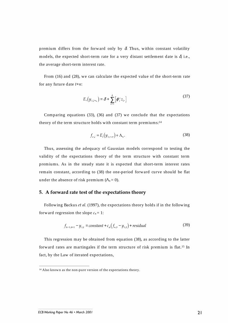
premium differs from the forward only by δ. Thus, within constant volatility

models, the expected short-term rate for a very distant settlement date is δ, i.e.,

the average short-term interest rate.

From (16) and (28), we can calculate the expected value of the short-term rate

for any future date %:

W W Q L

Q

LW

L

N

11

, +=

= +∑ δ ϕ(37)

Comparing equations (33), (36) and (37) we conclude that the expectations

theory of the term structure holds with constant term premiums:14

! Q W W W Q Q, ,

+1 . (38)

Thus, assessing the adequacy of Gaussian models correspond to testing the

validity of the expectations theory of the term structure with constant term

premiums. As in the steady state it is expected that short-term interest rates

remain constant, according to (38) the one-period forward curve should be flat

under the absence of risk premium (ΛQ = 0).

( )%

Following Backus (1997), the expectations theory holds if in the following

forward regression the slope &Q = 1:

! & ! '#(Q W W Q Q W W− + − = + − +1 1 1 1, , , ,&' (39)

This regression may be obtained from equation (38), as according to the latter

forward rates are martingales if the term structure of risk premium is flat.15 In

fact, by the Law of iterated expectations,

14 Also known as the non-pure version of the expectations theory.


22

! !Q W W W W Q Q W Q W Q Q, , ,

+ + - + -1 1 1 1 1 . (40)

Subtracting the short-term interest rate to both sides of (40) and adding a

residual term, we get (39).16 A rejection of this hypothesis can be taken as

evidence that term premiums vary over time. It can be confirmed that the

theoretical values of &Q implied by the class of Gaussian models under analysis

must be equal to one. In fact, by definition, & ! ! ! !

! !Q

Q W W Q W W

Q W W

=− −

−− +1 1 0 0

0

, , , ,

, ,

, , given

that 1,W!0,W, where:

! ! ! ! Q W W Q W W Q Q

7 7

Q Q− + + −− − = + − − −1 1 0 0 1 1 0 1 1, , , ,, Γ Φ , (41)

! ! Q W W Q Q

7

Q Q, ,− = + − + −+ +0 1 1 0 1 1 Γ , (42)

Γ0 is the unconditional variance of and is given by the solution to

Γ ΦΓ Φ0 0= +7 , (43)

where is a diagonal matrix with elements equal to the variances. The solution

is given by

& & 7Γ Φ Φ0

1 = − ⊗−

. . (44)

Therefore, the slope of the forward regression will be:

&

Q

Q Q

7 7

Q Q

Q Q

7

Q Q

=+ − − −

+ − + −+ −

+ +

1 1 0 1 1

1 1 0 1 1

Γ Φ

Γ.

(45)

15 This is a generalisation of the result in Campbell (1997), chapter 11, derived assuming nullrisk premium.16 The term related to the slope of the term structure of term premium is included in the constant,as it is assumed to be constant.


23

For any affine model we have limQ

Q

7

7&

→∞

= =1 0 1

1 0 1

1ΓΓ

. In our class of Gaussian

models, from (28), &Q = 1, ∀ Q.

*

The identification of the factors with macroeconomic variables can, in

principle, be achieved by estimating a joint model for the term structure and the

macro-economic variable, with a common factor related to the latter.

Assuming that the short-term interest rate can be decomposed into the short-

term real interest rate (expressed in deviation from the mean and denoted by 1,W)

and the expected one-period ahead inflation rate, we have:

1, 1 1, 1 1( )W W W W

π+ + += + . (46)

In Remolona . (1998), nominal and indexed-bonds are used in order to

estimate the expected inflation rate. In our case, as there were no indexed bonds

in Germany, the inflation process has to be estimated jointly with the processes

for bond yields. For example, if inflation (in deviation from the mean, denoted by

πW) follows an AR(1) process:

1 1W W Wπ ρπ+ += + (47)

where (W+1 is white noise, the component of the short-term interest rate related to

the second factor may be considered as the one-period inflation expectation:

( )2, 1W W W W π ρπ+= = (48)

From (48) and (32) the value of the second factor in +1 is given by:

( ) ( ) ( )2, 1 1 2 1 1 2, 1W W W W W W W W π ρ π ρ ρπ ρ ρ+ + + + + += = = + = + (49)


24

Comparing equations (32) and (49), we can exactly identify the parameters of

the second factor with the parameters of the inflation process:

ρ ϕρ σ ε

==+ +

2

1 2 2 1(W W,

,(50)

and the following relationship between inflation and the second factor can be

obtained:

2,2

1W W

πϕ

= .(51)

The main problem with the procedure sketched above is that (47) is not

necessarily the optimal model for forecasting inflation. In fact, it is too simple

concerning its lag structure and also does not allow for the inclusion of other

macroeconomic information that market participants may use to form their

expectations of inflation.17 For example, information about developments in

monetary aggregates, commodity prices, exchange rates, wages and unit labour

costs, etc, may be used by market participants to forecast inflation and, thus, may

be reflected in the bond pricing process. However, a more complex model would

certainly not allow a simple identification of the factor.

Given the difficulty and shortcomings of such exercise we suggest, as an

alternative, testing for the leading indicator properties of W2 for inflation.

We set up a VAR model withlags (see Hamilton (1994), chapter 11):

1 1 ...W W S W S W µ− −= + + + + (52)

where W is ()x 1) and each of the L is a ()x )) matrix of parameters with generic

element denoted NM

L and W

~ ( , )0 .

17 A more general ARMA model would perhaps be necessary to model the dynamics of inflation.Nevertheless, given that ϕ2 is close to 1, equation (51) implies a loss of leading indicatorproperties of the second factor regarding inflation.


25

The vector W is defined as

2

W

W

W

π =

.

To test whether W2 has leading indicator properties for inflation we test the

hypothesis 10 12 12: ... 0S = = = . This is a test for Granger causality, i.e., a test of

whether past values of the factor along with past values of inflation better

“explain” inflation than past values of inflation alone. This of course does not

imply that bond yields cause inflation. Instead it means that W2 is possibly

reflecting bond market’s expectations as to where inflation might be headed.

In assessing the leading indicator properties of W2 , the Granger causality test

can be supplemented with an impulse-response analysis. The vector ( )

representation of the VAR is given by:

1 1 2 2 ...W W W W µ − −= + + Ψ + Ψ + . (53)

Thus the matrix V has the interpretation:

W V

V

W

+∂ = Ψ′∂

;

that is, the row , column * element of V identifies the consequences of a one-

unit increase in the *th variable’s innovation at date ((MW) for the value of the -th

variable at time %' (LWV), holding all other innovations at all dates constant.

A plot of row , column * element of V

,L W V

MW

+∂

∂,

as a function of 'is the impulse-response function. It describes the response

of (L W V, + ) to a one-time impulse in M W, , with all other variables dated or earlier

held constant.


26

Suppose that the date value of the first variable in the autoregression W2 is

higher than expected, so that (W is positive. Then

, 2 1 2 ,

2 1

ˆ ( | , , ,..., )L W V W W W W S L W V

W W

+ − − − +′ ′ ′∂ ∂

=∂ ∂

,

when is a diagonal matrix.18

Thus if W2 is a leading indicator of inflation, a revision in market expectations

of inflation , 2 1ˆ ( | , ,..., )

L W V W W W S + − −′ ′∂ should be captured by the marginal impact of

a shock to the innovation process in the equation for W2 .

+ $

Given that the factors determining the dynamics of the yield curve are non-

observable, a Kalman filtering and maximum likelihood procedure was the

method chosen for the estimation of the model. In order to estimate the

parameters, the model must be written in the linear state-space form. According

to equation (14) and exploiting the information on the homoskedasticity of

yields, the measurement or observation equation for the two-factor Gaussian

model may be written as:19

1,1, 1 11 22

1, ,, 1 2

2, 1,1 1

2 ,2

...... ... ... ...

( ) 0 0

...... ... ... ...

( ) 0 0

WW

W O WO W O O O

W O WO

O WO O

υ

υυ

υ

++

= + +

,

(54)

18 We use a Cholesky decomposition of the variance-covariance of the innovations to identify theshocks. We order inflation first in the VAR to reflect the idea that whereas inflation does notrespond, contemporaneously, to shocks to expectations, these may be affected bycontemporaneous information on inflation.19 In this way we adjust simultaneously the yield curve and the volatility curve, avoidingimplausible estimates for the latter.


27

where W O W1, ,,... are the zero-coupon yields at time with maturities * = 1, … ,

periods and W O W O W O W1 1 2, , , ,,... , , ,+ , are normally distributed i.i.d. errors, with zero

mean and standard-deviation equal to M

2 , of the measurement equation for each

interest rate considered, M M= , ( )2 2 2 2

1, 1 2, 22

1O M M M

σ σ+ = + ,

M M1 1, ,= and

M M2 2, ,= .

Following equations (27), the transition or state equation for the same model

is:

W

W

W

W

W

W

1 1

2 1

1

2

1

2

1

2

1 1

2 1

0

0

0

0,

,

,

,

,

,

+

+

+

+

=

+

ϕϕ

σσ

εε

,(55)

where ε1 1,W+ and ε 2 1,W+ are orthogonal shocks with zero mean and variances equal

to 1. In the appendix, the technical details on Kalman filtering and the maximum

likelihood procedure are presented. Additional to the recursive restrictions, the

parameters are estimated subject to the usual signal restrictions.20 For further

details see, for instance, Hamilton (1994, chapter 13) or Harvey (1990).

, '

The data used consist of two databases. The first comprises monthly averages of

nine daily spot rates for maturities of 1 and 3 months and 1, 2, 3, 4, 5, 7 and 10

years, between January 1986 and December 1998. These spot rates were

estimated from euro-mark short-term interest rates, obtained from Datastream,

and par yields of German government bonds, obtained from J.P. Morgan, using

the Nelson and Siegel (1987) and Svensson (1994) smoothing techniques. One-

20 The Kalman filtering and the maximum likelihood estimation were carried out using a Matlabcode. We are grateful to Mike Wickens for his help on the code.


28

period forward rates were calculated for this sample, which allowed the forward

regressions to be performed.21

The second data set covers a longer period, between September 1972 and

December 1998.22 However this sample includes only spot rates for annual

maturities between 1 and 10 years, excluding the 9-year maturity.

The inflation rate was computed as the difference to the mean of the yearly

inflation rate, obtained from Datastream.

#&('

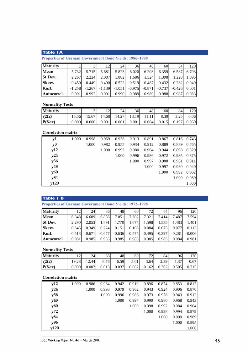
The properties of the German yield curve for both data sets are summarised in

Table 1. A number of features are worth noting. Firstly, between 1986 and 1998,

the term structure is negatively slopped at the short end, in contrast with the

more familiar concave appearance observed for the USA market (see, Backus

(1997)). Secondly, yields are very persistent, with monthly autocorrelations

above 0.98 for all maturities.23 Thirdly, yields are highly correlated along the

curve, but correlation is not equal one, suggesting that non-parallel shifts of the

yield curve are important. Therefore, one-factor models seem to be insufficient to

explain the German term structure of interest rates. As expected, the volatility

curve of yields is downward sloping.

+''!,&',

Figures 1 (Simple test) and 2 (Forward regressions) show the results of the

tests of the expectations theory of the term structure mentioned in the paper,

respectively equations (38) and (39). The pure expectations theory is easily

rejected: as shown in Figure 1 average one-period short-term forward rates vary

with maturity, which contradicts equation (38) in the steady state. By contrast,

21 We are grateful to Fátima Silva for research assistance on this issue.22 We are grateful to Manfred Kremer from the Research Department of the Bundesbank forproviding the data.23 Interest rates are close to being non-stationary.


29

forward regressions shown in Figure 2 generate slope coefficients close to one for

all maturities with relatively small standard errors,24 suggesting that the

assumption of constant term premiums is a reasonable approximation.

-!'('

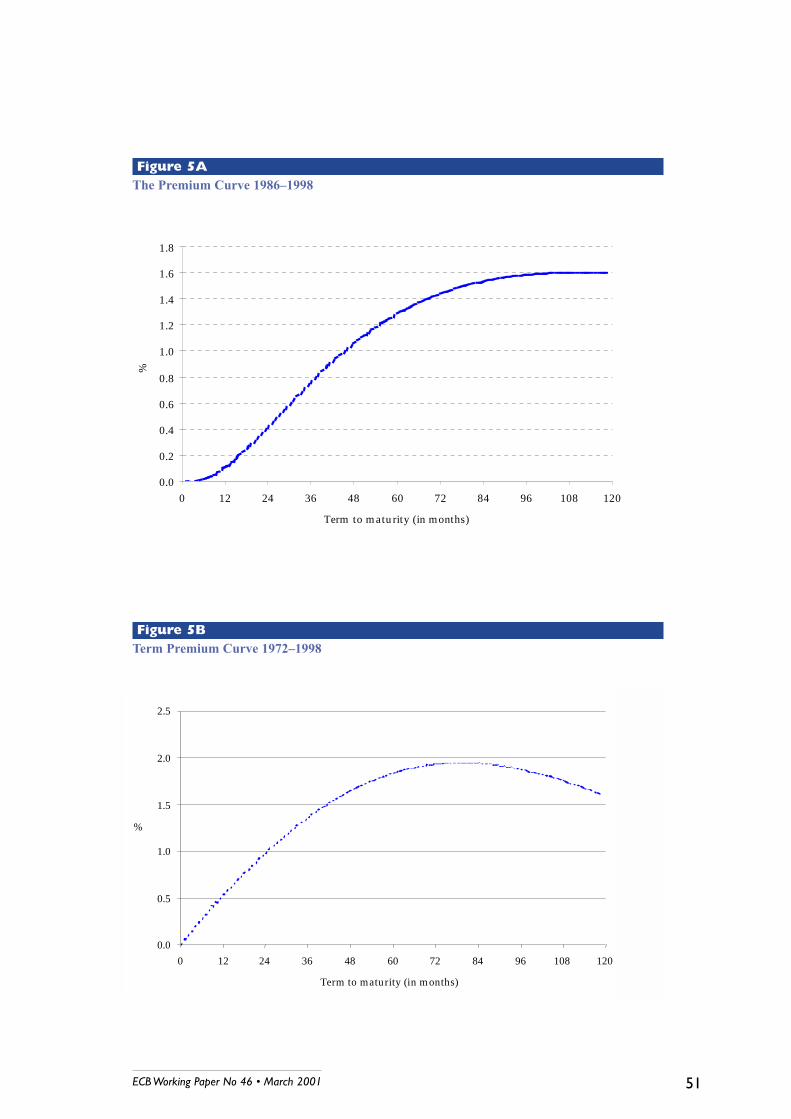
The results of the estimation are shown in Figures 3a and 3b (average nominal

yield curves), 4a and 4b (Volatility curves), 5a and 5b (Term premium curves), 6a

and 6b (One-period forward curves), 7a and 7b (Expected short-term interest rate

curves), 8a and 8b (Time-series yields), 9a and 9b (Factor loadings) and 10a, 10b,

10c, 10d, (Time-series factors). The parameters and respective standard errors are

reported in Table 2.

The estimates reproduce very closely both the average yield and the volatility

curves and generates plausible term premium curves. The estimates also

reproduce very closely the time-series of the yields across the whole maturity

spectrum.25 It is interesting to note that the fit is poorer at the end of the sample,

in 1998, when long bond yields fell (more than predicted by the model) as a

consequence of the Russian and Asian crisis, whilst short-rates remained

relatively stable (and above values predicted by the model).

Focusing on the estimates of the parameters, as the estimated ϕ ’s are close to

one and exhibit low volatility the factors are very persistent.26 Note that

standard-deviations are very low and thus confidence intervals are extremely

24 Newey-West standard errors.25 The quality of the fit for the yields contrasts with the results in Gong and Remolona (1997c). Forthe US at least two different two-factor heteroskedastic models are needed to model the wholeUS term structures of yields and volatilities: one to fit the medium/short end of the curves andanother to fit the medium/long term. The lowest time-series correlation coefficients is 0.87, forthe 10-year maturity, and the cross-section correlation coefficients are, in most days of thesample, above 0.9.26 Nevertheless, given that standard-deviations are low, the unit root hypothesis is rejected and,consequently, the factors are stationary. We acknowledge the comments of Jerome Henry on thisissue.


30

narrow.27 This confirms the high sensitivity of the shapes of the average and

volatility term structures to parameter estimates.28 It is the second factor that

contributes positively to the term premium and exhibits higher persistence.

Figures 9a and 9b show the factor loadings. The first factor is relatively more

important for the dynamics of the short end of the curve, and the second is

relatively more important for the long end of the curve.

Figures 10a, 10b, 10c, and 10d show the time-series of the unobservable factors

and proxies for the economic variables with which they are supposed to be

correlated – the real interest rate and the inflation rate. A first feature worth

mentioning is the correlation between the factors and the corresponding

economic variables.

Using $' real interest rates as proxies for the - real rates, the

correlation coefficients between one-month and three-month real rates and the

first factor is around 0.75. In the larger sample the correlation coefficient is 0.6.

Correlation between the second factor and inflation is close to 0.7 and 0.5,

respectively in the shorter and in the larger sample.

.##&'!!&)!!

We start with simple descriptive statistics. Table 3 shows cross-correlation

between W

π and W2 in the larger sample. If

W2 is a leading indicator for W

π then

the highest (positive) correlation should occur between lead values of W

π and W2 .

The shaded figures in the table are the correlation coefficients between W2 and

lags of W

π . The first figure in each row is and the next corresponds to the

27 Standard-deviations were computed from the variance-covariance matrix of the estimators (seeHamilton (1994), pp. 389, for details), using a numerical procedure.28 Very low standard-deviations for the parameters have been usually obtained in former Kalmanfilter estimates of term structure models, as Babbs and Nowman (1998), Gong and Remolona(1997a), Remolona . (1998) and Geyer and Pichler (1996).


31

correlation between W N

π − and W2 (negative means lead). The next to the right is

the correlation between 1W Nπ − − and

W2 , etc.

The correlation analysis is indicative of leading indicator properties of W2 .

Firstly, note that the highest correlation (in bold) is at the fourth lead of inflation

and, secondly, that correlation increases with leads of inflation up to lead 4 and

steadily decline for lags of inflation.

Table 4 presents the Granger causality test and Figure 11 the impulse-response

functions. The results strongly support the conjecture that W2 has leading

indicator properties for inflation. At the 5% level of confidence one can reject that

W2 does not Granger cause inflation. This is confirmed by the impulse-response

analysis.

A positive shock to the innovation process of W2 is followed by a statistically

significant increase in inflation. However a positive shock to the innovation

process of inflation does not seem to be followed by a statistically significant

increase in W2 . These results suggest that an innovation to the inflation process is

not “news” for the process of expectation formation. This is very much in

accordance with the (forward-looking) interpretation of shocks to W2 as reflecting

“news” about the future course of inflation.

Overall our results suggest that inflation expectations influence long-term

rates. Similar results concerning the information content of the German term

structure regarding future changes in inflation rate were obtained in previous

papers, namely Schich (1996), Gerlach (1995) and Mishkin (1991), using different

samples and testing procedures.29

29 Mishkin (1991) and Jorion and Mishkin (1991) results on Germany are contradictory as,according to Mishkin (1991), the short-end of the term structure does not contain information onfuture inflation for all OECD countries studied, except for France, United Kingdom and


32

-

The identification of the factors that determine the time-series and cross-section

behaviour of the term structure of interest rates is one of the most challenging

research topics in finance. As German yield data seems to support the

expectations theory with constant term premiums, we used a constant volatility

model to fit the term structure of interest rates in Germany.

We have shown that a two-factor models describes quite well the dynamics

and the shape of the German yield curve between 1972 and 1998. Reasonable

estimates are obtained also for the term premium and the volatility curves. Two

factors seem to drive the German term structure of interest rates: one factor

related to the $ real interest rate and a second factor linked to inflation

expectations.

Germany. Conversely, Jorion and Mishkin (1991) conclude that the predictive power of theshorter rates about future inflation is low in the U.S., Germany and Switzerland.Fama (1990) and Mishkin (1990a and 1990b) present identical conclusions concerning theinformation content of U.S. term structure regarding future inflation and state that the U.S. dollarshort rates have information content regarding future real interest rates and the longer ratescontain information on inflation expectations. Mishkin (1990b) also concludes that for severalcountries the information on inflation expectations is weaker than for the United States. Mehra(1997) presents evidence of cointegration between the nominal yield on 10-year Treasury Bondand the actual U.S. inflation rate. Koedijk and Kool (1995), Mishkin (1991) and Jorion andMishkin (1991) supply some evidence on the information content of the term structureconcerning the inflation rate in several countries.


33

%% ). /

The Kalman Filter is an algorithm that computes the optimal estimate for the

state variables at a moment using the information available up to $/. When the

parameters of the model are also unknown, as it is the case of our problem, they

are usually estimated by a maximum likelihood procedure.

The starting point for the derivation of the Kalman filter is to write the model in

state-space form, as in equations (54) and (55):

Observation or measurement equation:

(A1) 0 1 2W

OO U

W

UO N

W

N

W

O2 1 2 1 2 1 1× × × × × ×= ⋅ + ⋅ +

State or transition equation:

(A2) 1 3 1 4 W

NN N N

W

NN N

W

N× × × −× × ×

= + ⋅ +1 1

11 1

where 2 is the number of variables to estimate (being the number of terms

considered in the estimation), is the number of observable exogenous variables

and is the number of non-observable exogenous variables (the factors). Besides

the parameters that form the elements of , 0, and 3, it is also required to

estimate the elements of the variance-covariance matrix of the residuals of

equations (A1) and (A2):

(A3) 5 2 2O O

W W×= ’

(A4) 6 N N

W W×

+ +=

1 1 ’


34

In our two-factor model is a column vectorwith elements M W, for the first

rows ( = 9 ), and 1

2 12

12

22

22

M M, ,σ σ+ for the next rows;

W is a 2-dimension

column vector of one’s ( = 1), is a column vector of zeros and 3 is a

× diagonal matrix, with typical element 3LL L

= ϕ ( = 2 ). The values of the

elements of these matrices may be time-varying or constant, being in this case

known or unknown. In our model, they are constant and unknown.

The estimation departs from assuming that the starting value of the state vector 1

is obtained from a normal distribution with mean Rand variance 0.

R can be

seen as a guess concerning the value of 1 using all information available up to

and including = 0. As the residuals are orthogonal to the state variables,Rcannot be obtained using the data and the model. 0 is the uncertainty about

the prior on the values of the state variables.

Using 1

Rand 0 and following (A2), the optimal estimator for 11 will be given by:

(A5) |1 311 0 0= +

Consequently, the variance-covariance matrix of the estimation error of the state

vector will correspond to:

(A6)

1 1 1 1

31 4 31 31 4 31

3 4 3 4

3 3 4 4

3 3 46 4

1 0 1 1 0 1 1 0

0 1 0 0 1 0

0 1 0 1

0 0 1 1

1 0 1

| | |

|

’

’

’ ’ ’ ’

’ ’ ’ ’

’ ’

= − −

= + + − − + + − −

= + +

= += +

Given that = ⊗ ⋅’ , 1|0 may be obtained from:


35

(A7)

& & 3 3 & 46 4

3 3 & 4 4 & 6

3 3 4 4 & 6U U

1 0 1 0 1

1 0 1

1

12 2

| |

|

’ ’

= +

= ⊗ ⋅ + ⊗ ⋅

= − ⊗

⊗ ⋅

×

−

Generalising equations (A5) and (A6), we have the following prediction

equations:

(A8) |1 31W W W− −= +1 1

(A9) 3 3 46 4W W W W W| | ’ ’− −= +1 1

As 2W is independent from W and from all prior information on and (denoted

by ζW−1), we can obtain the forecast of W conditional on W and ζ

W−1 directly from

(A1):

(A10) 01W W W W W W| ,

|ζ − −= +1 1

Therefore, from (A1) and (A10), we have the following expression for the forecast

error:

(A11) 01 2 01 0 1 1 2W W W W W W W W W W W W W W

− = + + − + = − +− − −| , | |ζ 1 1 1

Given that 2W is also independent from 1W and |

W W−1 and considering (A11), the

conditional variance-covariance matrix of the estimation error of the observation

vector will be:

(A12)

0 1 1 2 0 1 1 2

0 1 1 1 1 0 2 2

0 0 5

W W W W W W W W W W W W W W W W

W W W W W W W W

W W

− − = − + − + =

= − − +

= +

− − − −

− −

−

| , | , ’ ’

’ ’ ’

’

| |

| |

|

ζ ζ1 1 1 1

1 1

1


36

In order to characterise the distribution of the observation and state vectors, it is

also required to compute the conditional covariance between both forecasting

errors. From (A11) we get:

(A13)

1 1 0 1 1 2 1 1

0 1 1 1 1

0

W W W W W W W W W W W W W W W

W W W W W W

W W

− − = − + −

= − −

=

− − − −

− −

−

| , | , ’ ’

’

| |

| |

|

ζ ζ1 1 1 1

1 1

1

Therefore, using (A10), (A12) and (A13), the conditional distribution of the vector

W W, is:

(A14) 1

0

10 0 5 0

0 W W W

W W W

W W W

W W

W W W W

W W W W

| ,| ,

~ ,’’

|

|

| |

| |

ζζ

−

−

−

−

− −

− −

+

+

1

1

1

1

1 1

1 1

According to a well-known result (see, Mood . (1974, pp. 167-168)), if 1and

2 have a joint normal conditional distribution characterised by

(A15)

1

2

1

2

11 12

21 22

~ ,

µµ

Ω ΩΩ Ω

then the distribution of 2 1| is ,Σ , with

(A16) = + −−µ µ2 21 111

1 1Ω Ω

(A17) Σ Ω Ω Ω Ω= − −22 21 11

112

Equations (A16) and (A17) correspond to the optimal forecast of 2 given 1

and to the mean square error of this forecast respectively. Consequently,

following (A14), the distribution of 1W given W, W and ζW−1 is 1

W W W W

,| | , where

|1W W

and W W| are respectively the optimal forecast of 1W given W_W and the mean


37

square error of this forecast, corresponding (using (A16) and (A17)) to the

following updating equations of the Kalman Filter:

(A18) ’ ’| | | | |1 1 0 0 0 5 0W W W W W W W W W W W W

= + + − +− − −

−

−1 1 1

1

1

(A19) 0 0 0 5 0W W W W W W W W W W| | | | |’ ’= − +− − −

−

−1 1 1

1

1

After estimating |

W W and

W W| , we can proceed with the estimation of |

W W+1 and

W W+1| . Considering (A8) and (A9), we obtain:

(A20) ’ ’

’ ’

| | | | | |

| | | |

1 31 3 1 0 0 0 5 0

31 3 0 0 0 5 0

W W W W W W W W W W W W W W

W W W W W W W W W W

+ − − −

−

−

− − −

−

−

= + = + + + − +

= + + + − +

1 1 1 1

1

1

1 1 1

1

1

(A21)

3 3 46 4

3 0 0 0 5 0 3 46 4

3 3 3 0 0 0 5 0 3 46 4

W W W W W

W W W W W W W W W

W W W W W W W W W

+

− − −

−

−

− − −

−

−

= +

= − + +

= − + +

1

1 1 1

1

1

1 1 1

1

1

| |

| | | |

| | | |

’ ’

’ ’ ’ ’

’ ’ ’ ’ ’

The matrix 3 0 0 0 5W W W W| |’ ’− −

−+1 1

1 is usually known as the gain matrix, since it

determines the update in

W W+1| due to the estimation error of W. The equation

(A21) is known as a Ricatti equation. Concluding, the Kalman Filter may be

applied after specifying starting values for 1|0 and 1|0 using equations (A10),

(A12), (A18), (A19) and iterating on equations (A20) and (A21).

The parameters are estimated using a maximum likelihood procedure. The log-

likelihood function corresponds to:

(A22) log log |. 7 ! 7 W W

W

7

= −=∑ 1

1


38

being

(A23)

! 0 0 5 01 0 0 5 01W W W W W W W W W W W W| ’ exp ’ ’

| | | |−−

−

−

− −

−

−= + ⋅ − − − + − −

1

1 21

1 2

1 1

1

1212

π

for = 1, …, +.

The estimation procedure may be resumed as follows:


39

(if there are(if all iterations iterations to be done) are done)

(if the maximum hasn’t(if the maximum for the been obtained) sum has been obtained)

END

matrices (A, H, C, F, R, Q) Starting values for the parameter

log-likelihood function (A22)

New value for Y (A10)

(A5) and for P1|0 (A7)New value for S

Value of the log-likelihood

error of the observation equation (A12)Variance matrix of the estimation

Forecasting the new values forS (A20) and P (A21)

Starting values for the state vector S

Sum of the values of the

Forecasting error of Y (A11)

Updating S (A18) and P (A19)

errors of both equations (A13)Conditional covariance between the

function (A23)

$#%


40

0

Aït-Sahalia, Yacine (1996), “Testing Continuous-Time Models of the Spot Interest

Rate”, 52!3&1(#', No. 9, pp. 427-70.

Babbs, Simon H. and K. Ben Nowman (1998), “An Application of Generalized

Vasicek Term Structure Models to the UK Gilt-edged Market: a Kalman Filtering

analysis”, #3&&&', No. 8, pp. 637-644.

Backus, David, Silverio Foresi and Chris Telmer (1998), ''Discrete-Time Models of

Bond Pricing'', NBER Working paper No. 6736.

Backus, David, Silverio Foresi, Abon Mozumdar and Liuren Wu (1997),

“Predictable Changes in Yields and Forward Rates”, .

Balduzzi, Pierluigi, Sanjiv Ranjan Das, Silverio Foresi and R. Sundaram (1996),

“A Simple Approach to Three Factor Affine Term Structure Models”, 8( !

3#&, No.6, pp. 43-53, December.

Bliss, Robert (1997), “Movements in the Term Structure of Interest Rates”,

Federal Reserve Bank of Atlanta, &&52, Fourth Quarter.

Buhler, Wolfgang, Marliese Uhrig-Homburg, Ulrich Walter and Thomas Weber

(1999), “An Empirical Comparison of Forward-Rate and Spot-Rate Models for

Valuing Interest-Rate Options”, +,8(!3&, Vol. LIV, No.1, February.

Campbell, John Y., Andrew W. Lo and A. Craig MacKinlay (1997), +,

&&'!3&', Princeton University Press.

Campbell, John Y. (1995), “Some Lessons from the Yield Curve”, 8( !

&&'&', Vol. 9, No. 3, pp. 129-152.


41

Chen, R. and L. Scott (1993a), “Maximum Likelihood Estimations for a Multi-

Factor Equilibrium Model of the Term Structure of Interest Rates”, 8( !

3#&, No. 3, pp. 14-31.

Chen, R. and L. Scott (1993b), “Multi-Factor Cox-Ingersoll-Ross Models of the

Term Structure: Estimates and Test from a Kalman Filter”, Working Paper,

University of Georgia.

Cox, John, Jonathan Ingersoll and Stephen Ross (1985), “A Theory of the Term

Structure of Interest Rates”, &&, No. 53, pp. 385-407.

Dai, Qiang and Kenneth J. Singleton (1998), “Specification Analysis of Affine

Term Structure Models”, .

Deacon, Mark and Andrew Derry (1994), “Deriving Estimates of Inflation

Expectations from the Prices of UK Government Bonds”, Bank of England

9 23.

De Jong, Frank (1997), “Time-Series and Cross-section Information in Affine

Term Structure Models”, Center for Economic Research Working Paper.

Duffie, Darrell (1992), : &''&+, , Princeton University Press.

Duffie, Darrell and Rui Kan (1996), ''A Yield Factor Model of Interest Rates'',

,&3&, No. 6, pp. 379-406.

Fama, Eugene F. (1990), “Term Structure Forecasts of Interest Rates, Inflation and

Real Returns”, 8(! &&', No. 25, pp. 59-76.

Fleming, Michael J. and Eli M. Remolona (1998), “The Term Structure of

Announcement Effects”, .


42

Fung, Ben Siu Cheong, Scott Mitnick and Eli Remolona (1999), “Uncovering

Inflation Expectations and Risk Premiums from Internationally Integrated

Financial Markets”, W.P. 99-6, Bank of Canada.

Gerlach, Stefan (1995), “The Information Content of the Term Structure: Evidence

for Germany”, BIS Working Paper No. 29, September.

Geyer, Alois L. J. and Stefan Pichler (1996), “A State-Space Approach to Estimate

and Test Multifactor Cox-Ingersoll-Ross Models of the Term Structure”, .

Gong, Frank F. and Eli M. Remolona (1997a), “A Three-factor Econometric Model

of the US Term Structure” FRBNY 1!!5', No. 19, Jan.1997.

Gong, Frank F. and Eli M. Remolona (1997b), “Inflation Risk in the U.S. Yield

Curve: The Usefulness of Indexed Bonds”, Federal Reserve Bank of New York,

June, .

Gong, Frank F. and Eli M. Remolona (1997c), “Two factors along the yield curve”

+,&,'1&,1(, pp. 1-31.

Hamilton, James D. (1994), + 1' '', Princeton (NJ), Princeton

University Press.

Harvey, Andrew C. (1990), 3&'; 1(&( +$1' #' # ,

-3, Cambridge University Press.

Jorion, P. and Frederic Mishkin (1991), “A multicountry comparison of term-

structure forecasts at long horizons”, 8( ! 3& &&', No. 29, pp.

59-80.

Koedijk, K. G. and C. J. M. Kool (1995), “Future inflation and the information in

international term structures”, &&&', No. 20, pp. 217-242.


43

Litterman, Robert and José Scheinkman (1991), ''Common Factors Affecting Bond

Returns'', 8(!3#& 1, June, pp. 49-53.

Mehra, Yash P. (1997), “The Bond Rate and Actual Future Inflation”, Federal

Reserve Bank of Richmond, Working Paper Series, W.P. 97-3, March.

Mishkin, Frederic (1990a), “What does the term structure tell us about future

inflation”, 8(! &&', No. 25, pp. 77-95.

Mishkin, Frederic (1990b), “The information in the longer maturity term

structure about future inflation”, 6( 8(!&&', No. 55, pp. 815-

828.

Mishkin, Frederic (1991), “A multi-country study of the information in the

shorter maturity term structure about future inflation”, 8( !

#3&, No. 10, pp. 2-22.

Mood, A. (1974) (3rd ed.) #(&,+, !1'&', International

Student Edition, McGraw-Hill.

Nelson, Charles R. and Andrew F. Siegel (1987) - "Parsimonious Modelling of

Yield Curves", 8(!(''', 1987, Vol. 60, No. 4.

Remolona, Eli, Michael R. Wickens and Frank F. Gong (1998), “What was the

market’s view of U.K. Monetary Policy? Estimating Inflation Risk and Expected

Inflation with Indexed Bonds”, FRBNY 1!!5', No. 57, December 1998.

Ross, Stephen A. (1976), “The arbitrage theory of capital asset pricing”, 8(!

&&+, , No. 13, pp. 341-360.

Schich, Sebastian T. (1996), “Alternative Specifications of the German Term

Structure and its Information Content Regarding Inflation”, Deutsche

Bundesbank, Discussion Paper 8/96.


44

Svensson, Lars E.O. (1994) - "Estimating and Interpreting Forward Interest Rates:

Sweden 1992-4", CEPR :'&(''1' No. 1051.

Vasicek, Oldrich (1977), “An equilibrium characterisation of the term structure”,

8(!3&&&', No. 5, pp. 177-188.

Wong, F. (1964), “The construction of a class of stationary Markov processes”, in

Bellman, R. (Ed.), 1&,'& &''' ,& , '&' # ,

Proceedings of Symposia in Applied Mathematics, Vol. 16, American

Mathematical Society, Providence, R.I., pp. 264-276.

Zin, Stanley (1997), “Discussion of Evans and Marshall”, $5&,'

!&(<&& , November.


45

5 1 3 12 24 36 48 60 84 1205 5.732 5.715 5.681 5.823 6.020 6.203 6.359 6.587 6.7931' 3 2.267 2.224 2.087 1.882 1.686 1.524 1.398 1.228 1.0951# 0.450 0.449 0.490 0.522 0.519 0.487 0.432 0.282 0.049 -1.258 -1.267 -1.139 -1.051 -0.975 -0.871 -0.737 -0.426 0.001 0.991 0.992 0.991 0.990 0.989 0.989 0.988 0.987 0.983

6.

5 1 3 12 24 36 48 60 84 120χ2(2) 15.56 15.67 14.68 14.27 13.19 11.11 8.39 3.25 0.062789): 0.000 0.000 0.001 0.001 0.001 0.004 0.015 0.197 0.969

)

1.000 0.998 0.969 0.936 0.913 0.891 0.867 0.816 0.743& 1.000 0.982 0.955 0.934 0.912 0.889 0.839 0.765! 1.000 0.993 0.980 0.964 0.944 0.898 0.829!; 1.000 0.996 0.986 0.972 0.935 0.875&* 1.000 0.997 0.988 0.961 0.911;, 1.000 0.997 0.980 0.940*< 1.000 0.992 0.962,; 1.000 0.989!< 1.000


Table 1AProperties of German Government Bond Yields: 19861998

Table 1 BProperties of German Government Bond Yields: 19721998

5 12 24 36 48 60 72 84 96 1205 6.348 6.609 6.856 7.051 7.202 7.321 7.414 7.487 7.5941' 3 2.290 2.053 1.891 1.770 1.674 1.598 1.535 1.483 1.4011# 0.545 0.349 0.224 0.151 0.108 0.084 0.075 0.077 0.112 -0.513 -0.671 -0.677 -0.636 -0.575 -0.495 -0.397 -0.281 -0.006 0.981 0.985 0.985 0.985 0.985 0.985 0.985 0.984 0.981

6.

5 12 24 36 48 60 72 84 96 120χ2(2) 19.28 12.44 8.76 6.59 5.01 3.64 2.39 1.37 0.672789): 0.000 0.002 0.013 0.037 0.082 0.162 0.302 0.505 0.715

)

! 1.000 0.986 0.964 0.942 0.919 0.896 0.874 0.853 0.812!; 1.000 0.993 0.979 0.962 0.943 0.924 0.906 0.870&* 1.000 0.996 0.986 0.973 0.958 0.943 0.912;, 1.000 0.997 0.990 0.980 0.968 0.943*< 1.000 0.998 0.992 0.984 0.964+! 1.000 0.998 0.994 0.979,; 1.000 0.999 0.989-* 1.000 0.995!< 1.000

46

δ σ1 ϕ1 λ1σ1 σ2 ϕ2 λ2σ2-,*--, 0.00489 0.00078 0.95076 0.22192 0.00173 0.98610 -0.09978-+!--, 0.00508 0.00127 0.96283 0.10340 0.00165 0.99145 -0.10560


Table 2 AParameter estimates

Monthly Data From 1972:09 To 1998:12

Correlation between W N

π − and W2 (i.e. negative means lead)

-25: 0.3974759 0.4274928 0.4570631 0.4861307 0.5129488 0.5394065

-19: 0.5639012 0.5882278 0.6106181 0.6310282 0.6501370 0.6670820

-13: 0.6829368 0.6979626 0.7119833 0.7235875 0.7324913 0.7385423

-7: 0.7432024 0.7453345 0.7457082 <+;(,!- 0.7443789 0.7411556

-1: 0.7368274 0.7311008 0.7144727 0.6954511 0.6761649 0.6561413

5: 0.6360691 0.6159540 0.5949472 0.5726003 0.5478967 0.5229193

11: 0.4960254 0.4706518 0.4427914 0.4156929 0.3870690 0.3590592

17: 0.3311699 0.3011714 0.2720773 0.2425888 0.2126804 0.1829918

23: 0.1527293 0.1226024 0.0927202 0.0636053 0.0362558 0.0085952

29: -0.0167756 -0.0421135 -0.0673895 -0.0911283 -0.1139021 -0.1356261

Table 3Cross correlations of series t and z2t

Table 2 BStandard deviation estimates

δ σ1 ϕ1 λ1σ1 σ2 ϕ2 λ2σ2-,*--, 0.00009 0.00001 0.00142 0.00648 0.00003 0.00100 0.00084-+!--, 0.00001 0.00001 0.00000 0.00000 0.00249 0.00084 0.00013

47

. ; Granger causality tests

Inflation does not Granger cause Z2

Variable F-Statistic Significance

Wπ 5.8 0.03 *Z2 does not Granger cause inflation

Variable F-Statistic Significance Z2 6.12 0.03 *

* Means rejection at 5% level


Table 4Granger causality tests

48

5.0

5.5

6.0

6.5

7.0

7.5

8.0

0 12 24 36 48 60 72 84 96 108 120

%


0.85

0.90

0.95

1.00

1.05

1.10

0 12 24 36 48 60 72 84 96 108 120

Maturity (in months)

Bet

a

0.85

0.90

0.95

1.00

1.05

1.10

Figure 1Simple test of the pure expectations theory of interest ratesForward rate average curve 19861998

Figure 2Test of the expectations theory of interest ratesForward regression coefficient 19861998

3 12 24 36 48 60 84 120β 0.953 0.965 0.975 0.980 0.981 0.981 0.980 0.979

σ(β) 0.029 0.022 0.015 0.013 0.012 0.012 0.013 0.014α -0.003 0.005 0.020 0.029 0.034 0.038 0.043 0.046

σ(α) 0.007 0.019 0.025 0.030 0.033 0.036 0.040 0.043

49

5.0

5.5

6.0

6.5

7.0

7.5

8.0

0 12 24 36 48 60 72 84 96 108 120

Term to maturity (in months)

%

Observed 2f non-id.


Figure 3AAverage Nominal Yield Curve 19861998

5.0

5.5

6.0

6.5

7.0

7.5

8.0

0 12 24 36 48 60 72 84 96 108 120


%

Observed 2f non-id.

Figure 3BAverage Yield Curve 19721998

Estimated

Estimated


0.0

0.5

1.0

1.5

2.0

2.5

3.0

0 12 24 36 48 60 72 84 96 108 120


Stan

dar

d-d

ev. o

f Y

ield

s

Observed 2f non-id.

Figure 4AVolatility Curve 19861998

0.0

0.5

1.0

1.5

2.0

2.5

3.0

0 12 24 36 48 60 72 84 96 108 120


Stan

dar

d-d

ev. o

f Y

ield

s

Observed 2f non-id.

Figure 4BVolatility Curve 19721998

Estimated

Estimated

ECB Working Paper No 46 March 2001 51

0.0

0.2

0.4

0.6

0.8

1.0

1.2

1.4

1.6

1.8

0 12 24 36 48 60 72 84 96 108 120


%

Figure 5AThe Premium Curve 19861998

0.0

0.5

1.0

1.5

2.0

2.5

0 12 24 36 48 60 72 84 96 108 120


%

Figure 5BTerm Premium Curve 19721998


5.0

5.5

6.0

6.5

7.0

7.5

8.0

8.5

9.0

0 12 24 36 48 60 72 84 96 108 120

Time to settlement (in months)

%

Figure 6AAverage Forward Curve 19861998

5.0

5.5

6.0

6.5

7.0

7.5

8.0

8.5

9.0

0 12 24 36 48 60 72 84 96 108 120

Time to settlement (in months)

%

Figure 6BAverage Forward Curve 19721998

ECB Working Paper No 46 March 2001 53

5.0

5.2

5.4

5.6

5.8

6.0

6.2

6.4

6.6

6.8

7.0

0 12 24 36 48 60 72 84 96 108 120

Horizon (in months)

%

Figure 7AAverage Expected Short-term Interest Rate 19861998

6.00

6.05

6.10

6.15

6.20

6.25

6.30

0 12 24 36 48 60 72 84 96 108 120

Horizon (in months)

%

Figure 7BAverage Expected Short-term Interest Rate 19721998

54 ECB Working Paper No 46 March 2001

Figure 8ATime-series yield estimation results 19861998

PRQWK

0

2

4

6

8

10

12

14

1986

1987

1988

1989

1990

1991

1992

1993

1994

1995

1996

1997

1998

observed 2f non-id.

\HDU

0

2

4

6

8

10

12

14

1986

1987

1988

1989

1990

1991

1992

1993

1994

1995

1996

1997

1998

observed 2f non-id.

\HDU

0

2

4

6

8

10

12

14

1986

1987

1988

1989

1990

1991

1992

1993

1994

1995

1996

1997

1998

observed 2f non-id.

\HDU

0

2

4

6

8

10

12

14

1986

1987

1988

1989

1990

1991

1992

1993

1994

1995

1996

1997

1998

observed 2f non-id.

\HDU

0

2

4

6

8

10

12

14

1986

1987

1988

1989

1990

1991

1992

1993

1994

1995

1996

1997

1998

observed 2f non-id.

\HDU

0

2

4

6

8

10

12

14

1986

1987

1988

1989

1990

1991

1992

1993

1994

1995

1996

1997

1998

observed 2f non-id.

Estimated Estimated

Estimated Estimated


Figure 8BTime-series yield estimation results 19721998

\HDU

0

2

4

6

8

10

12

14

1972

1973

1974

1975

1976

1977

1978

1979

1980

1981

1982

1983

1984

1985

1986

1987

1988

1989

1990

1991

1992

1993

1994

1995

1996

1997

1998

observed 2f non-id.

\HDU

0

2

4

6

8

10

12

14

1972

1973

1974

1975

1976

1977

1978

1979

1980

1981

1982

1983

1984

1985

1986

1987

1988

1989

1990

1991

1992

1993

1994

1995

1996

1997

1998

observed 2f non-id.

\HDU

0

2

4

6

8

10

12

14

1972

1973

1974

1975

1976

1977

1978

1979

1980

1981

1982

1983

1984

1985

1986

1987

1988

1989

1990

1991

1992

1993

1994

1995

1996

1997

1998

observed 2f non-id.

\HDU

0

2

4

6

8

10

12

14

1972

1973

1974

1975

1976

1977

1978

1979

1980

1981

1982

1983

1984

1985

1986

1987

1988

1989

1990

1991

1992

1993

1994

1995

1996

1997

1998

observed 2f non-id.

\HDU

0

2

4

6

8

10

12

14

1972

1973

1974

1975

1976

1977

1978

1979

1980

1981

1982

1983

1984

1985

1986

1987

1988

1989

1990

1991

1992

1993

1994

1995

1996

1997

1998

observed 2f non-id.

\HDU

0

2

4

6

8

10

12

14

1972

1973

1974

1975

1976

1977

1978

1979

1980

1981

1982

1983

1984

1985

1986

1987

1988

1989

1990

1991

1992

1993

1994

1995

1996

1997

1998

observed 2f non-id.

Observed Estimated Observed Estimated



56

0.0

0.2

0.4

0.6

0.8

1.0

1.2

0 12 24 36 48 60 72 84 96 108 120Term to maturity (in months)

%

F1 non-id. F2 non-id.


Figure 9AFactor loadings in the two-factor models 19861998

0.0

0.2

0.4

0.6

0.8

1.0

1.2

0 12 24 36 48 60 72 84 96 108 120Term to maturity (in months)

%

F1 non-id. F2 non-id.

Figure 9BFactor loadings in the two-factor models 19721998

Factor 1 Factor 2

Factor 1 Factor 2

57

-6

-4

-2

0

2

4

6

Jan-

86

Jan-

87

Jan-

88

Jan-

89

Jan-

90

Jan-

91

Jan-

92

Jan-

93

Jan-

94

Jan-

95

Jan-

96

Jan-

97

Jan-

98

Rea

l int

eres

t ra

tes

(%)

-0.15

-0.1

-0.05

0

0.05

0.1

0.15

Fact

ors

1m.Real Rate 3m.Real Rate Non-ident.


Figure 10ATime-series evolution of the 1st. factor 19861998

-4

-3

-2

-1

0

1

2

3

4

5

6

Sep

-72

Sep

-74

Sep

-76

Sep

-78

Sep

-80

Sep

-82

Sep

-84

Sep

-86

Sep

-88

Sep

-90

Sep

-92

Sep

-94

Sep

-96

Sep

-98

Rea

l int

eres

t ra

tes

(%)

-0.6

-0.4

-0.2

0

0.2

0.4

0.6

Fact

ors

1m. Real Rate 3m. Real Rate Non-ident.

Figure 10BTime-series evolution of the 1 st. factor 19721998

Factor

Factor

58

-4

-3

-2

-1

0

1

2

3

4

Jan-

86

Jan-

87

Jan-

88

Jan-

89

Jan-

90

Jan-

91

Jan-

92

Jan-

93

Jan-

94

Jan-

95

Jan-

96

Jan-

97

Jan-

98Non-ident. Yearly CPI


Figure 10CTime-series evolution of the 2nd. factor 19861998

Figure 10DTime-series evolution of the 2nd. factor 19721998

-6

-4

-2

0

2

4

6

Sep

-72

Sep

-74

Sep

-76

Sep

-78

Sep

-80

Sep

-82

Sep

-84

Sep

-86

Sep

-88

Sep

-90

Sep

-92

Sep

-94

Sep

-96

Sep

-98

non-ident. Yearly CPI

Factor

Factor

5954

RESP. OF PI TO PISIZE= 5%

2 4 6 8 10 12 14 16 18 200.00

0.05

0.10

0.15

0.20

0.25

0.30

0.35

0.40

RESP. OF Z2 TO PISIZE= 5%

2 4 6 8 10 12 14 16 18 20-0.15

-0.10

-0.05

0.00

0.05

0.10

0.15

0.20

0.25

0.30

RESP. OF PI TO Z2SIZE= 5%

2 4 6 8 10 12 14 16 18 200.0

0.1

0.2

0.3

0.4

0.5

RESP. OF Z2 TO Z2SIZE= 5%

2 4 6 8 10 12 14 16 18 200.08

0.16

0.24

0.32

0.40

0.48

0.56

0.64


Figure 11Impulse-response functions and two standard error bankds

European Central Bank Working Paper Series

1 A global hazard index for the world foreign exchange markets by V. Brousseau and F. Scacciavillani, May 1999.

2 What does the single monetary policy do? A SVAR benchmark for the European CentralBank by C. Monticelli and O.Tristani, May 1999.

3 Fiscal policy effectiveness and neutrality results in a non-Ricardian world by C. Detken, May1999.

4 From the ERM to the euro: new evidence on economic and policy convergence among EU countries by I.Angeloni and L. Dedola, May 1999.

5 Core inflation: a review of some conceptual issues by M.Wynne, May 1999.

6 The demand for M3 in the euro area by G. Coenen and J.-L.Vega, September 1999.

7 A cross-country comparison of market structures in European banking by O. de Bandt and E. P. Davis, September 1999.

8 Inflation zone targeting by A. Orphanides and V.Wieland, October 1999.

9 Asymptotic confidence bands for the estimated autocovariance and autocorrelation func-tions of vector autoregressive models by G. Coenen, January 2000.

10 On the effectiveness of sterilized foreign exchange intervention by R. Fatum,February 2000.

11 Is the yield curve a useful information variable for the Eurosystem? by J. M. Berk and P. van Bergeijk, February 2000.

12 Indicator variables for optimal policy by L. E. O. Svensson and M.Woodford,February 2000.

13 Monetary policy with uncertain parameters by U. Söderström, February 2000.

14 Assessing nominal income rules for monetary policy with model and data uncertainty by G. D. Rudebusch, February 2000.

15 The quest for prosperity without inflation by A. Orphanides, March 2000.

16 Estimating the implied distribution of the future short term interest rate using the Longstaff-Schwartz model by P. Hördahl, March 2000.

17 Alternative measures of the NAIRU in the euro area: estimates and assessment by S. F. and R. Mestre, March 2000.

18 House prices and the macroeconomy in Europe: Results from a structural VAR analysis by M. Iacoviello,April 2000.


19 The euro and international capital markets by C. Detken and P. Hartmann,April 2000.

20 Convergence of fiscal policies in the euro area by O. De Bandt and F. P. Mongelli,May 2000.

21 Firm size and monetary policy transmission: evidence from German business survey data by M. Ehrmann, May 2000.

22 Regulating access to international large value payment systems by C. Holthausenand T. Rønde, June 2000.

23 Escaping Nash inflation by In-Koo Cho and T. J. Sargent, June 2000.

24 What horizon for price stability by F. Smets, July 2000.

25 Caution and conservatism in the making of monetary policy by P. Schellekens, July 2000.

26 Which kind of transparency? On the need for clarity in monetary policy-making by B.Winkler,August 2000.

27 This is what the US leading indicators lead by M. Camacho and G. Perez-Quiros,August 2000.

28 Learning, uncertainty and central bank activism in an economy with strategic interactionsby M. Ellison and N.Valla,August 2000.

29 The sources of unemployment fluctuations: an empirical application to the Italian case by S. Fabiani,A. Locarno, G. Oneto and P. Sestito, September 2000.

30 A small estimated euro area model with rational expectations and nominal rigidities by G. Coenen and V. Wieland, September 2000.

31 The disappearing tax base: Is foreign direct investment eroding corporate income taxes? by R. Gropp and K. Kostial, September 2000.

32 Can indeterminacy explain the short-run non-neutrality of money? by F. De Fiore,September 2000.

33 The information content of M3 for future inflation by C.Trecroci and J. L.Vega,October 2000.

34 Capital market development, corporate governance and the credibility of exchange ratepegs by O. Castrén and T.Takalo, October 2000.

35 Systemic risk:A survey by O. De Bandt and P. Hartmann, November 2000.

36 Measuring core inflation in the euro area by C. Morana, November 2000.

37 Business fixed investment: Evidence of a financial accelerator in Europe by P.Vermeulen,November 2000.


38 The optimal inflation tax when taxes are costly to collect by F. De Fiore, November 2000.

39 A money demand system for euro area M3 by C. Brand and N. Cassola, November 2000.

40 Financial structure and the interest rate channel of ECB monetary policy by B. Mojon,November 2000.

41 Why adopt transparency? The publication of central bank forecasts by P. M. Geraats, January2001.

42 An area-wide model (AWM) for the euro area by G. Fagan, J. Henry and R. Mestre,January 2001.

43 Sources of economic renewal: from the traditional firm to the knowledge firm by D. R. Palenzuela, February 2001.

44 The supply and demand for eurosystem deposits The first 18 months by U. Bindseil and F.Seitz, February 2001.

45 Testing the Rank of the Hankel matrix: a statistical approach by G. Camba-Mendez and G. Kapetanios, February 2001.

46 A two-factor model of the German term structure of interest rates by N. Cassola and J. B. Luís, February 2001.


A two-factor model of the German term structure of interest rates

Documents

Transcript of A two-factor model of the German term structure of interest rates