The Determinants of the Benchmark Interest Rates in China: A Discrete Choice Model Approach

The Determinants of the Benchmark Interest Rates in China:

A Discrete Choice Model Approach∗

Hyeongwoo Kim† and Wen Shi‡

August 2016

Abstract

This paper empirically investigates the determinants of the two key benchmark interest

rates in China using an array of constrained ordered probit models for quarterly frequency data

from 1987 to 2013. Specifically, we estimate the behavioral equation of the People’s Bank of

China that models its decision-making process for revisions of the benchmark deposit rate and

the lending rate. Our findings imply that the PBC’s policy decisions are better understood

as responses to changes in inflation and money growth, while output gaps and the exchange

rate play negligible roles. We also implement in-sample fit analyses and out-of-sample forecast

exercises. Our empirical findings show robust and reasonably good performances of our models

in understanding dynamics of these benchmark interest rates.

Keywords: Monetary Policy; People’s Bank of China; Ordered Probit Model; Deposit

Rate; Lending Rate; In-Sample Fit; Out-of-Sample Forecast

JEL Classification: E52; E58

∗We thank seminar participants at the 2014 WEAI conference for helpful suggestions. A special thank goes toWeibo Xiong for generously providing his data.†Department of Economics, Auburn University, 0339 Haley Center, Auburn, AL 36849. Tel: (334) 844-2928. Fax:

(334) 844-4615. Email: [email protected].‡Contact Author: Wen Shi, Department of Accounting & Finance, Turner College of Business, Columbus State

University, Columbus, GA 31907. Tel: (706) 507-8150. Fax: (706) 568-2184. Email: [email protected].

1

1 Introduction

China is one of the fastest growing economies and has been considered as a new engine of world

growth for many years. Naturally, the People’s Bank of China (PBC) has received great attention

from the public regarding when and to how it would revise the target benchmark interest rates. In

the present paper, we attempt to estimate the behavioral function of the PBC. To put it differently,

we attempt to understand how they determine the two policy interest rates: the benchmark deposit

rate and the lending rate.

As is well documented, the PBC appears to have employed combinations of multiple policy

instruments that include both the monetary and interest rate instruments (Xie, 2004; Peng, Chen,

and Fan, 2006; Geiger, 2008; Zhang, 2009; Liu and Zhang, 2010; Xiong, 2012; Giardin, Lunven,

and Ma, 2014; Sun, 2013). Among others, we pay a special attention on the PBC’s benchmark

interest rates, because those interest rates have been consistently employed as policy instruments

with no break since 1986 (Xiong, 2012). Also, as shown by He and Wang (2012), market interest

rates in China have been heavily influenced by these benchmark rates.

We acknowledge that the PBC will eventually allow these regulated interest rates to be deter-

mined mainly by market forces. However, it is highly likely that the PBC would employ another

interest rate targets, such as the target (range) federal funds rate in the US, in a more market

oriented economic system in the future. Therefore, studying the decision making process for revi-

sions of these interest rates would provide useful information on how the PBC will determine their

monetary policy stance in the future.

One popular approach to study the PBC’s interest rate setting behavior is based on a Taylor

rule-type model that assumes the PBC revises the target interest rate continuously. Since the work

of Xie and Luo (2002) who employed the Taylor Rule to study China’s monetary policy, Zhao and

Gao (2004), Bian (2006), Wang and Zou (2006), and more recently, Fan, Yu, and Zhang (2011)

estimated similar versions of linear Taylor rule models, while Zhang and Zhang (2008), Ouyang

and Wang (2009), Chen and Hou (2009), Zheng, Wang, and Guo (2012), and Jawadi, Mallick, and

Sousa (2014) used nonlinear models for China’s monetary policy.

It should be noted, however, that the Monetary Policy Committee (MPC) under the PBC

normally meets every quarter, 4 times a year, to make decisions on the monetary policy stance.

Further, it turns out that the PBC revised their benchmark interest rates with a less than 30%

frequency based on 106 quarterly observations since 1987. Such a high degree inertia in dynamics of

the policy interest rates calls for an alternative approach in studying the monetary policy decision-

making process in China.

Since the seminal work of Dueker (1999), many researchers have employed a discrete choice

model framework to study the monetary policy stance of the Federal Reserve System in the US.

For example, Hamilton and Jordà (2002) used the autoregressive conditional hazard (ACH) model

in combination with the ordered probit model. Hu and Phillips (2004a,b) extended the work of

Park and Phillips (2000) to a nonstationary discrete choice model, and studied the monetary policy

decision-making process in Canada and the US, respectively. On the other hand, Kim, Jackson,

2

and Saba (2009) used Hu and Phillips’models to implement out-of-sample forecast exercises for the

Fed’s interest rate setting behavior. Using a similar discrete choice model, Monokroussos (2011)

reported structural changes in the U.S. monetary policy reaction function estimates around the

pre- and the post Volcker eras. Also, Gerlach (2007) employed a discrete choice model framework

to study policy actions of the European Central Bank (ECB), while Kim, Shi, and Hwang (2016)

investigated interest rate setting behavior of the Bank of Korea.

There are a few papers that study the monetary policy stance decision-making process of the

PBC using qualitative response models. He and Pauwels (2008) constructed a monetary policy

stance index using multiple policy instruments. Then they studied how macroeconomic and finan-

cial variables explain realized policy actions that are measured by changes in this policy stance

variable.1 Constructing a refined policy stance index variable for a longer sample period, Xiong

(2012) investigated the PBC’s decision making process using a similar discrete choice model.2

Unlike these researches, we take a direct approach to study dynamics of specific policy instru-

ments instead of monetary policy index variables that are constructed by authors. Put it differently,

we study policy decision-marking processes of the PCB in revising the benchmark interest rates

that are actually observable to the public. Therefore, our analysis could provide practically more

useful information to the market participants. In contrast to He and Pauwels (2008) and Xiong

(2012), we employ a constrained ordered probit model that allows policy makers to revise the in-

terest rate only when the going interest rate deviates suffi ciently from a newly calculated optimal

interest rate.

Using quarterly frequency data from 1987 to 2013, we estimate an array of discrete choice

models for China’s monetary policy decision making process. Our findings highlight important and

statistically significant roles of inflation and money growth rate in determination of the benchmark

interest rates in China, while output gaps and the foreign exchange rate play negligible roles. In-

sample fit analyses and out-of-sample forecast exercises demonstrate quite robust and reasonably

good performances of our models.

The rest of the paper is organized as follows. Section 2 examines advantages and disadvantages

of using other policy instruments to identify the monetary policy stance in China. In Section

3, we describe the econometric model employed in the present paper. Section 4 provides a data

description and preliminary test results that highlight empirical justification of using discrete choice

models. Section 5 reports our probit model estimation results and in-sample fit analyses. In Section

6, we discuss our out-of-sample forecast exercise results. Section 7 concludes.

1 Instead of using actual data, they extracted multiple latent common factor components from a big set of macro-economic and financial variables via the method proposed by Bai and Ng (2004).

2He and Pauwels (2008) use the ordered probit model that allows covariates to be nonstationary (Hu and Phillips,2004a,b), whereas Xiong (2012) employs the conventional discrete choice model where all covariates are stationary.

3

2 Policy Instruments of Monetary Policy in China

As we mentioned briefly in the previous section, the PBC has employed an array of policy instru-

ments. This section provides short descriptions on those instruments, then discusses the merits of

investigating the policy decision-making process on the target benchmark interest rates in compar-

ison with alternative instruments.

PBC’s major policy instruments include the required reserve ratio (RRR), the benchmark de-

posit and lending rates, and central bank bills (short-term bonds) that the PBC has used for open

market operations (OMO) since 2002. Changes in the monetary policy stance via these instruments

are normally observable because the PBC announces their actions to the public, sometimes prior to

effective dates. The PBC also adopts policy instruments that may not be readily observable such

as foreign exchange interventions, window guidance, and administrative measures.3

The RRR is a quantity-based instrument that helps manage banking system liquidity intro-

duced in 1998 (He and Pauwels, 2008; Xiong, 2012). RRR is not a popularly employed instrument

in advanced economies, because its effect on the money supply is too strong for small-scale adjust-

ments. Interestingly, the PBC made a lot more frequent changes in RRR than in the commercial

bank benchmark deposit and lending rates during times of financial market turmoil.

That is, as we can see in Table 1, the PBC made 20 revisions in RRR after the recent financial

crisis in September 2008, while they revised the benchmark rates only 8 times. These actions sharply

contrast with their earlier behavior prior to the Asian financial crisis in 1998. As we can see in

Figure 1, RRR virtually stays constant until around 1998. That is, they used the benchmark lending

and deposit rates more frequently than RRR during tranquil periods of time. This probably reflects

the severity of the Great Recession triggered by the recent financial crisis. To put it differently,

it might be the case that the PBC had to rely heavily on RRR which generates more powerful

impacts on credit markets than the benchmark interest rates. However, revisions in RRR are

normally consistent with those in the benchmark interest rates as they exhibit comovements (see

Figure 1) over time, which implies that the PBC has combined these policy instruments.

Table 1 and Figure 1 around here

The PBC started conducting OMO on a regular basis in 2002, which helped reducing the stock

of outstanding central bank bills that has increased substantially due to PBC’s sterilization of

heavy inflows of the foreign exchanges into China (He and Pauwels, 2008). Also, the PBC often

used OMO in combination with RRR by absorbing excess market liquidity from maturing central

bank bills into required reserves by raising RRR.

3Foreign exchange interventions are often used to control movements of yuan in the forex market. Window guidancenormally gives nonbinding advices to financial institutions regarding their target credit growth and desirable financialresource allocations. Administrative measures are often used to control the speed of commercial loan growth.(He andPauwels,2008)

4

Notwithstanding the significantly important roles of RRR and OMO in understanding the mon-

etary policy decision-making process in China, we are particular interested in the PBC’s commercial

bank benchmark deposit and lending rates because they have been consistently employed as policy

instruments with no break since 1986 compared with RRR and OMO.

We also acknowledge that various kinds of monetary aggregate variables are used in the literature

to measure the monetary policy stance in China (Xie, 2004; Burdekin and Siklos, 2008; Koivu,

2008). However, changes in the monetary base, M1, or M2 reflect money demand shocks as well as

the monetary policy shock. Furthermore, changes in monetary aggregates are greatly influenced by

foreign factors or export revenues. The PBC typically attempts to sterilize these changes, but their

sterilization procedures may not be entirely successful, which means measuring the policy stance

via innovations in monetary aggregates could be a challenge.

In addition, the monetary targets announced by the PBC may not serve an appropriate proxy

of the monetary policy stance, because, as He and Pauwels (2008) point out, these targets are

announced at an annual frequency with no frequent revisions. Further, Liao and Tapsoba (2014)

report the stable relationship between the money demand, output, and interest rates disappears

after 2008 due to rapid financial innovation and liberalization, which implies a more important role

of price-based monetary targets such as interest rates in conducting monetary policy.

We recognize that PBC has carried out interest rate reforms toward a more market-orientated

system. This does not necessarily mean that the PBC will never attempt to influence market interest

rates. Since January 2013, the PBC started using new policy tools such as short-term liquidity

operations (SLO), standing lending facility (SLF), the medium-term lending facility (MLF), and

pledged supplementary lending (PSL).

Under a more market-oriented financial system, we believe that the PBC will target short-

run interest rates, paying attention on interest rates in the medium to the long-term, which is in

line with the federal reserve system’s strategy. Therefore, the present paper that investigates the

behavioral function of the PBC regarding its determination of optimal interest rates would provide

useful information in predicting the PBC’s actions in the future.

3 The Econometric Model

The People’s Bank of China (PBC) is assumed to set an optimal interest rate (i∗t ) based on exoge-

nous macroeconomic variables (xt) that are observed at time t. i∗t is not directly observable to the

public. That is, it is a latent variable. We model this by the following linear equation.

i∗t = x′tβ − εt, (1)

where β is a k × 1 vector of coeffi cient and εt denotes a scalar error term.

We assume that the PBC revises the benchmark interest rate (it) only when the newly calculated

optimal interest rate i∗t in (1) deviates suffi ciently from the prevailing interest rate in the previous

period (it−1). For this, we define the following deviation variable of i∗t from it−1,

5

y∗t = i∗t − it−1, (2)

where y∗t is also a latent variable. Note that the greater y∗t is (in absolute value), the stronger the

incentive to revise it would be. This framework has been first employed by Dueker (1999), then

by Hu and Phillips (2004a, 2004b) and Kim, Jackson and Saba (2009), whereas He and Pauwels

(2008) and Xiong (2012) used conventional ordered probit models with no such mechanism. Xiong

employed a lagged policy stance variable instead, even though he failed to find significant coeffi cient

estimates for that variable.

We employ a trichotomous discrete choice model. That is, we assume that the PBC chooses one

of the following three policy actions: cut the interest rate (C), let it stay where it is (S), or raise

the interest rate (H), which implies a three-regime model that requires two threshold variables, τLand τU .

For this, let’s denote yt the observable policy varible that takes discrete values. When y∗t is

less than the lower threshold (τL), it would indicate that the PBC should cut the interest rate

(yt = −1). A difference greater than the upper threshold (τU ) would require an interest rate hike

(yt = 1), and any minor deviation between τL and τU , an inaction band, would indicate that the

PBC will choose S (yt = 0). Formally,

yt =

−1,

0,

1,

if

if

if

y∗t < τL

τL ≤ y∗t ≤ τUy∗t > τU

: C

: S

: H

(3)

and

Ij,t =

yt(yt−1)

2 ,

1− y2t ,yt(yt+1)

2 ,

if

if

if

j = C

j = S

j = H

(4)

where Ij,t is the indicator function for each of the realized policy index variables (yt).

The log likelihood function for a random sample of size T , {yt}Tt=1, is the following.

L =

T∑t=1

[Ic,t lnPc (xt : θ) + Is,t lnPs (xt : θ) + Ih,t lnPh (xt : θ)] (5)

where θ is the parameter vector (β, τ). The probability function Pj is defined as follows.

Pj =

1− F

(x′tβ − it−1 − τL

),

F(x′tβ − it−1 − τL

)− F

(x′tβ − it−1 − τU

),

F(x′tβ − it−1 − τU

),

if

if

if

j = C

j = S

j = H

(6)

We assume that F (·) is the standard normal (or logistic) distribution function. That is, we em-ploy the constrained trichotomous ordered probit (or logit) model where the coeffi cient on it−1 is

6

restricted to be −1.

4 Data and Preliminary Analysis

4.1 Data Description

We use quarterly frequency observations that span from 1987:I to 2013:IV. As Xiong (2012) pointed

out, the PBC has been using a set of policy instruments that includes its marginal refinancing

facility, benchmark interest rates, and the required reserve ratio. We focus on the determination of

the two benchmark interest rates in China, the lending rate and the deposit rate, which have been

continuously employed by the PBC for key instruments since 1986.4

We plot these two interest rates in the first panel of Figure 2. It should be noted that these

rates are infrequently revised. Among 106 quarterly observations, there were 14 cuts and 14 hikes

for the benchmark deposit rate (second panel), while 15 cuts and 16 hikes were observed for the

lending rate (third panel). That is, the PBC chose "stay" decisions with over 70% frequency,

which implies that the PBC revises the rates only when its perceived optimal interest rate deviates

suffi ciently from the prevailing rate. The ordered probit model described earlier thus seems to

be appropriate for estimating such discrete actions. Corresponding trichotomous discrete choice

variables (yt = −1, 0, 1) are reported in the last two panels.

We also note that these interest rates exhibit highly persistent dynamics. In response to the

Asian financial crisis in 1997:IV, the deposit rate declined from 7.47% to 5.67% and the lending

rate went down from 10.08% to 8.64%. The rates continued to decrease for about 8 years, then

started to increase from 2004:IV until the beginning of the recent financial crisis in 2008. In what

follows, we show that linear models such as the Taylor rule, which often rely on the ordinary least

squares (OLS) estimator, may not be appropriate to study the interest rate setting behavior of the

PBC under such circumstances, because the OLS estimator may not perform well in the presence

of highly persistent (possibly nonstationary) data.

Figure 2 around here

Inflation (πt) is the quarterly log difference of the All Items Consumer Price Index (CPI). For

the output gap (yt), we consider the following two measures: the quadratically detrended real

industrial production index (yQt ) and the Hodrick-Prescott (HP) filtered cyclical component of the

real industrial production index (yHt ), setting the smoothing parameter at 1,600 for quarterly data.

Money growth rate (∆mt) is the quarterly log difference of the M1. The appreciation rate of

Chinese Yuan (∆st) is the quarterly log difference of the nominal effective exchange index. All

interest rates are divided by 4 to make them conformable to these quarterly growth rates. The

4Given the benchmark lending rate, commercial banks set their interest rates based on their credit assessment oftheir customers. The deposit interest rate is the rate paid by banks on demand, time, or savings accounts.

7

CPI data is from the Organization for Economic Cooperation and Development (OECD), and real

industrial production index is from the Economist Intelligence Unit (EIU) and the National Bureau

of Statistics in China. All other data are obtained from the International Financial Statistics (IFS).

We report graphs of these macroeconomic covariates in Figure 3.


4.2 Unit Root Tests

We implement the augmented Dickey-Fuller (ADF) test for all variables used in the study. Results

are reported in Table 2.

The test fails to reject the null hypothesis of nonstationarity for the primary lending rate and

the deposit rate even at the 10% significance level, which seems to be consistent with their highly

persistent movements shown in Figure 2. Note that the OLS estimator is not appropriate when

some variables in regression equations are nonstationary. The ordered probit model employed

in this paper, however, can avoid such problems, since the trichotomous policy index variable

yt = {−1, 0, 1} is used instead of potentially nonstationary interest rates.It should be also noted that the MLE estimation for the ordered probit/logit model may yield

wrong standard errors if covariates are nonstationary. The procedure proposed by Hu and Phillips

(2004a,b) applies in such cases. Since the ADF test strongly rejects the null of nonstationarity for all

covariates irrespective of the specification of deterministic components, we employ the conventional

MLE instead of Hu and Phillips’method.

Table 2 around here

4.3 Linear Taylor Rule Model Estimations

We perform another preliminary analysis by estimating an array of Taylor rules using the OLS

method as follows.

it = α+ γππt−1 + γyyt−1 + Θxt−1 + εt (7)

where xt−1 is either a scalar or a vector of additional explanatory variables. γπ and γy denote the

long-run coeffi cients that help infer how the central bank responds to innovations in inflation and

the output gap, respectively. Following Xiong (2012), we assume that policy makers can access

information on the macroeconomic covariate variables with one quarter lag. We also implement

estimations for Taylor rules with the interest rate smoothing consideration (see Clarida, Galí, and

Gertler, 2000, for example) as follows.

it = α+ γsππt−1 + γsy yt−1 + Θsxt−1 + ρit−1 + εt (8)

8

Note that the short-run coeffi cients γsπ and γsy and the smoothing parameter ρ in (8) jointly imply

γπ = γsπ/(1− ρ) and γy = γsy/(1− ρ) in (7).

All estimation results for (7) and (8) are reported in Table 3. We note that the coeffi cient

on inflation is always highly significant at the 1% level, while that of the output gap is mostly

insignificant. All other explanatory variables are also insignificant. Further, yt−1 and ∆st−1 often

have incorrect signs.5

We also note that these estimates violate the Taylor principle (γπ > 1) no matter what spec-

ifications are used. For example, the implied long-run inflation coeffi cient is about 0.40 and 0.60

for the lending rate and the deposit rate, respectively. Furthermore, we noticed that the degree of

interest rate inertia, measured by ρ in (8), is close to one, which implies that the interest rates obey

a near unit root process. If the interest rates are nonstationary as is implied by the ADF test in

the previous section, the OLS estimates presented in Table 3 might not be appropriate. The probit

model estimates in the following section, however, does not have such a problem since we use the

policy index variable which assumes discrete numbers.

Table 3 around here

5 Probit Model Estimation and In-Sample Fit Analysis

This section reports our estimates for the probit model described earlier. Our benchmark model

(Model 1) is motivated by the Taylor Rule with an assumption that the policy-makers observe

inflation and the output gap with one period lag. Extended models with additional covariates are

also considered. That is, Models 2 and 3 include ∆mt−1 and ∆st−1, respectively, in addition to the

Taylor Rule variables πt−1 and yt−1. Model 4 is the full model that includes all key macroeconomics

covariates. Results are provided in Table 4.

Major findings are roughly tri-fold. First, all threshold estimates are highly significant at any

conventional levels, which imply that the PBC revises the benchmark lending and deposit rates

only when there are substantial deviations of the current rate from the optimal rate. Second, the

coeffi cient estimate on inflation is always significant, while the output gap coeffi cient estimates

are all insignificant. Third, Models 2 and 4 estimations show that money growth coeffi cient is

significant at least at the 10% level, while the yuan appreciation rate (∆st−1) coeffi cient estimates

are always insignificant.

These results suggest inflation and money growth rate play important roles in the PBC’s interest

rates decision-making process, which is consistent with findings by He and Pauwels (2008) and Xiong

5Depreciations (decreases in∆st−1) tend to make inflationary pressure build up, which implies a negative coeffi cienton ∆st−1.

9

(2012) who also reported an important role of inflation in understanding the monetary policy stance

in China.6

Table 4 around here

We implement a robustness check analysis to see how stable these coeffi cient estimates are over

the sample period. For this purpose, we recursively estimate our models beginning with the first

half observations (1987:II to 2000:III), then repeat estimations by adding one observation in each

round until all observations are used. That is, we obtain 52 sets of coeffi cient estimates for each

model. We report the coeffi cient estimates along with their 95% confidence bands in Figure 4 for

the models 1 and 2.

The coeffi cient estimates from our recursive estimations are overall stable over time, which con-

firms the robustness of our full-sample estimates. The inflation coeffi cient estimates are significant

at the 5% level and the money growth rate coeffi cient estimates are mostly significant at the 10%

level. The output gap coeffi cient estimates are negligible and always statistically insignificant.


Next, we evaluate our ordered probit models for the PBC’s decision-making process in terms

of in-sample fit performance. For this purpose, we report correct prediction rates of our models in

Table 5. For the benchmark lending rate, Model 1 predicted 5 C decisions correctly out of 15 actual

cut decisions, resulting in a 33% success rate. The model correctly predicted 85% of S decisions,

while its prediction success rate for H decisions was 13%. Combining all results, Model 1’s overall

performance was 66%. Models 2, 3, and 4 performed similarly. Overall success rates for the deposit

rate were slightly higher for the deposit rate than those for the lending rate, though success rates

for C and H decisions were roughly similar.

Table 5 around here

Overall success rates are heavily influenced by high success rates for S decisions, which is about

85% for the lending rate and 92% for the deposit rate. On the other hand, our models predict C

and H decisions less successfully when we use the point estimates for τL and τU . Recognizing the

uncertainty around these point estimates for thresholds, we re-evaluate the in-sample performance

of our models as follows.6Shu and Ng (2010) use a narrative approach by compiling indices of the PBC’s policy stance on the basis of meeting

notes and the policy statements. They also find that the money growth rate and inflation are key determinants ofthe monetary policy in China.

10

Figure 5 plots the estimated latent variable y∗t from Models 2 for the lending rate and the

deposit rate, along with the estimates for τL and τU and their 95% confidence bands. Obviously,

a more compact inaction band such as [τL + 2 × std(τL), τU − 2 × std(τU )] will yield more C and

H predictions with a cost of lower success rates for S decisions. Such schemes would be desirable

when market participants are vigilant for possible changes in the monetary policy stance. Model

evaluation results with this alternative scheme are reported in Table 6.

We observe roughly similar in-sample fit performance. Even though the success rate for S

decisions declines in all models, our models perform much better for C and H decisions. For

instance, the success rate for C decisions improves to 53% for the lending rate, while the success

rate for H decisions goes up as high as 38%.

Figure 5 around hereTable 6 around here

Even though our alternative scheme improves the success rates for C and H decisions consider-

ably, the performance of our models still may not be considered satisfactory. Note that our models

predict C and H decisions only when y∗t deviates from the inaction band. In other words, our

models may fail to produce a warning signal even when y∗t approaches rapidly toward the threshold

values.

Recognizing this, we calculate and report the probability estimate of each policy intervention

using the coeffi cient estimates from Model 2. In Figure 6, the estimated probabilities are illustrated

with actual decisions (bar graphs) over the full sample period. These figures show that our models

trace changes in the probabilities fairly well. The probability of each event tends to rise rapidly

when corresponding actions take place. For instance, the probability of a C goes up rapidly during

the Asian financial crisis around in 1998. Also, the estimated probability of an H climbs up fast

around 2007 and 2011 when the PBC raised the interest rates several times.


It should be noted that estimated probabilities tend to be higher in the pre-2000 period com-

pared with those in the latter period. As can be seen in Figure 3, output gaps exhibit a big swing

in the pre-2000 period. Inflation was also extremely high and volatile in the pre-2000 period, which

required substantially bigger revisions of the benchmark interest rates as can be seen in Figure 2.

Since our model does not distinguish quantitative differences in the size of revisions, our models

tend to generate lower probabilities in the post-2000 period samples. However, our models are able

to pick up rapidly rising probabilities for hikes and cut decisions.

Our models generated very high probabilities of a hike decision in around 1994 for both bench-

mark interest rates. It turns out that the PBC used alternative instruments during that time.

11

That is, the growth rate of central bank refinancing to commercial banks decreased from 44.19% in

1993:III to 6.4% in 1994:IV. This implies that our models correctly predicted the monetary policy

stance during this period.

As to other possible mismatches between the predicted possibilities (probabilities) and the actual

decisions in these figures, we suggest an explanation based on the following institutional features

about the actual monetary policy decision-making process in China. Although the PBC might

propose that it was time to take certain policy actions based on macroeconomic or financial market

signals, the State Council might not be in a position to dispose in a timely manner because it makes

decisions based on consensus. In other words, other ministries (e.g. the National Development and

Reform Commission, the Ministry of Commerce, and the Ministry of Finance) will need to be

on board with the proposed change in monetary policy stance before the State Council makes a

decision. Therefore, there might be some substantial time lags between PBC’s proposals and the

State Council’s disposal, which may explain why actual decisions tend to lag our model predictions.

6 Out-of-Sample Forecasting

This section evaluates the out-of-sample predictability of our ordered probit models for the interest

rate setting behavior in China. Predicting the PBC’s revision decisions on these rates provides

crucially useful information not only to financial market participants but also entrepreneurs who

make important investment decisions.

We first implement our exercises by a recursive method with the first 50% observations as the

split point. The recursive forecasting approach begins with a memory window from the beginning of

the sample to 2000:III. That is, we start calculating one-period ahead forecast on the policy variable

(C, S, and H) using first 53 observations. Then adding the 54th observation, we re-estimate and

formulate the forecast of the next policy outcome with this expanded set of observations. We

continue to do this until we forecast the last policy action in 2013:III using the full sample data

from 1987:I to 2013:II.

As is well-known, the recursive forecasting strategy may not perform well if there are structural

changes in the underlying data generating process. To put it differently, if regime changes occur

some time during the early period of analysis, then including earlier data in the estimation could

reduce the forecastability of our model. To address this possibility, we also employ a fixed rolling

window approach described as follows.

Here we begin with the same initial 53 observations. After estimating and predicting the 54th

policy action, we add the 54th actual observation, but drop the 1st observation from the sample,

thereby retaining an updated 53-observation estimation window, which is used to produce the next

policy outcome, the 55th action. We repeat this procedure until we forecast the last policy outcome

variable using the last sample set of 53 observations.

We report calculated out-of-sample probabilities of cuts and hikes in Figures 7 and 8, for the

lending rate and the deposit rate, respectively. Realized C and H policies are also reported in bar

12

graph.

We note that the rolling window method performs better than the recursive method in our

experiment. The probability of a cut (C) increases faster with the rolling window scheme. Similarly,

the probability of a hike (H) rises rapidly reaching almost 100% with the rolling window, while

the highest probability with the recursive method was below 50%. We observed similar out-of-

sample forecast performance for the deposit rate. These findings suggest that some changes, either

gradual or abrupt, have occurred to the PBC’s interest rate setting behavior. In Figure 4, we noted

that inflation and money growth coeffi cients decreased steadily, which might have been caused

by relatively moderate movements of macroeconomic variables including inflation (see Figure 3).

Also, as we can see in Figure 2, revisions to the benchmark interest rates have been quite modest

in absolute sizes compared with earlier adjustments. All these observations imply that the PBC is

moving toward the direction of fine-tuning the interest rate.

Figures 7 and 8 around here

7 Concluding Remarks

This paper estimates the response function of the PBC to changes in macroeconomic variables as

to revisions of their benchmark interest rates: the deposit rate and the lending rate. We employ an

array of constrained ordered probit models for quarterly frequency data from 1987 to 2013, because

the conventional least squares estimator for Taylor rule type models may be inappropriate when

the policy interest rates show substantial degree inertia. Our preliminary analysis also justifies the

use of qualitative response models.

We find that the PBC’s interest rate setting behavior could be well-explained by discrete re-

sponses to changes in inflation and in money growth rate. Output gaps and the yuan appreciation

rate seem to play negligible and insignificant roles in determining revision decisions on these bench-

mark interest rates. We evaluated our models using an in-sample fit criteria, which demonstrated

fairly good performances. We also implemented out-of-sample prediction exercises, employing both

the recursive and the fixed-size rolling window schemes with initial 50% observations as a split

point. Our model performed fairly well especially when the rolling window method is used.

13

References

Bai, J., and S. Ng (2004): “A panic attack on unit roots and cointegration,”Econometrica, 72(4),

1127—77.

Bian, Z. (2006): “A review of empirical issues of Taylor rule and its applicability in China,”

Journal of Finance Research, 08, 56—69.

Burdekin, R. C., and P. L. Siklosb (2008): “What has driven Chinese monetary policy since

1990s? Investigating the People’s Bank’ s policy rule,” Journal of International Money and

Finance, 27(5), 847—859.

Chen, H., Q. Chen, and S. Gerlach (2011): “The implementation of monetary policy in

China:The internal market and bank lending,”HKIMR Working Paper, 26.

Chen, Y., and Z. Huo (2009): “A conjecture of Chinese monetary policy rule: Evidence from sur-

vey data, Markov regime switching, and drifting coeffi cients,”Annals of Economics and Finance,

10(1), 111—153.

Clarida, R., J. Galí, and M. Gertler (2000): “Monetary policy rules and macroeconomic

stability: Evidence and some theory,”The Quarterly Journal of Economics, 115(1), 147—180.

Dueker, M. (1999): “Measuring monetary policy inertia in target federal funds rate changes,”

Federal Reserve Bank of St Louis Review, 81(3-9).

Fan, L., Y. Yu, and C. Zhang (2011): “An empirical evaluation of China’s monetary policies,”

Journal of Macroeconomics, 33(2), 358—371.

Geiger, M. (2008): “Instruments of monetary policy in China and their effectiveness: 1994-2006,”

United Nations Conference on Trade and Development, No. 187.

Gerlach, S. (2007): “Interest rate setting by the ECB: Words and deeds,”International Journal

of Central Banking, 3(3), 1—46.

Girardin, E., S. Lunven, and G. Ma (2014): “Inflation and China’s monetary policy reaction

function: 2002-2013,”BIS Papers No. 77.

Hamilton, J. D., and Òscar Jordà (2002): “A model for the federal funds target rate,”Journal

of Political Economy, 110, 1135—1167.

He, D., and L. L. Pauwels (2008): “What prompts the people’s bank of china to change its

monetary policy stance? Evidence from a discrete choice model,” China & World Economy,

16(6), 1—21.

He, D., and H. Wang (2012): “Dual-track interest rates and the conduct of monetary policy in

China,”China Economic Review, 23(4), 928—47.

14

Hu, L., and P. C. B. Phillips (2004a): “Dynamics of the federal funds target rate: A nonsta-

tionary discrete choice approach,”Journal of Applied Econometrics, 19, 851—867.

(2004b): “Nonstationary discrete choice,”Journal of Econometrics, 120, 103—138.

Jawadi, F., S. K. Mallick, and R. M. Sousa (2014): “Nonlinear monetary policy reaction

functions in large emerging economies: The case of Brazil and China,” Applied Economics,

46(9), 973—984.

Kim, H., J. Jackson, and R. Saba (2009): “Forecasting the FOMC’s interest rate setting

behavior: A further analysis,”Journal of Forecasting, 28(2), 145—165.

Kim, H., W. Shi, and K.-M. Hwang (2016): “Estimating interest rate setting behavior in Korea:

A constrained ordered choices model approach,”Applied Economics, 48, 2199—2214.

Koivu, T. (2009): “Has the Chinese economy become more sensitive to interest rates? Studying

credit demand in China,”China Economic Review, 20(3), 455—470.

Liao, W., and S. J.-A. Tapsoba (2014): “China’s Monetary Policy and Interest Rate Liberal-

ization: Lessons from International Experiences,”IMF Working Paper 14/75.

Liu, L., and W. Zhang (2010): “A new Keynesian model for analysing monetary policy in

mainland China,”China Journal of Asian Economics, 21(6), 540—551.

Monokroussos, G. (2011): “Dynamic limited dependent variable modeling and US monetary

policy,”Journal of Money, Credit and Banking, 43(2-3), 519—534.

Ouyang, Z., and S. Wang (2009): “The asymmetric reaction of monetary policy to inflation and

real GDP in China,”Economic Research Journal, 9, 27—38.

Park, J. Y., and P. C. B. Phillips (2000): “Nonstationary binary choice,” Econometrica,

68(1429-1482).

Peng, W., H. Chen, and W. Fan (2006): “Interest rate structure and monetary policy imple-

mentation in mainland China,”China Economic Issues, 1-06.

Shu, C., and B. Ng (2011): “Monetary Stance and Policy Objectives in China: A Narrative

Approach,”HKMA China Economic Issues, 1/10.

Sun, R. (2013): “Does monetary policy matter in China? A narrative approach.,”China Economic

Review, 23, 56—74.

Wang, S., and H. Zou (2006): “Taylor’s rule in the condition of opening economy: To test the

monetary policy of China,”Statistical Research, 23, 42—47.

Xie, P. (2004): “China’s monetary policy:1998-2002,”Stanford Center for International Develop-

ment Working paper 217.

15

Xie, P., and X. Luo (2002): “Taylor rule and its empirical test in China’s monetary policy,”

Economic Research Journal, 3, 2—13.

Xiong, W. (2012): “Measuring the monetary policy stance of the People’s Bank of China: An

ordered probit analysis,”China Economic Review, 23, 512—533.

Zhang, W. (2009): “China’s monetary policy: Quantity versus price rules,”Journal of Macroeco-

nomics, 31(3), 473—84.

Zhang, Y., and D. Zhang (2008): “Interest rate rule with a role of money and its empirical test

in China,”Economic Research Journal, 12, 65—74.

Zhao, J., and H. Gao (2004): “Robust monetary policy rules in an environment of interest rate

liberalization in China,”China Economic Quarterly, 3, 41—64.

Zheng, T., X. Wang, and H. Guo (2012): “Estimating forward-looking rules for

China’smonetary policy: A regime-switching perspective,”China Economic Review, 23(2), 47—

59.

16

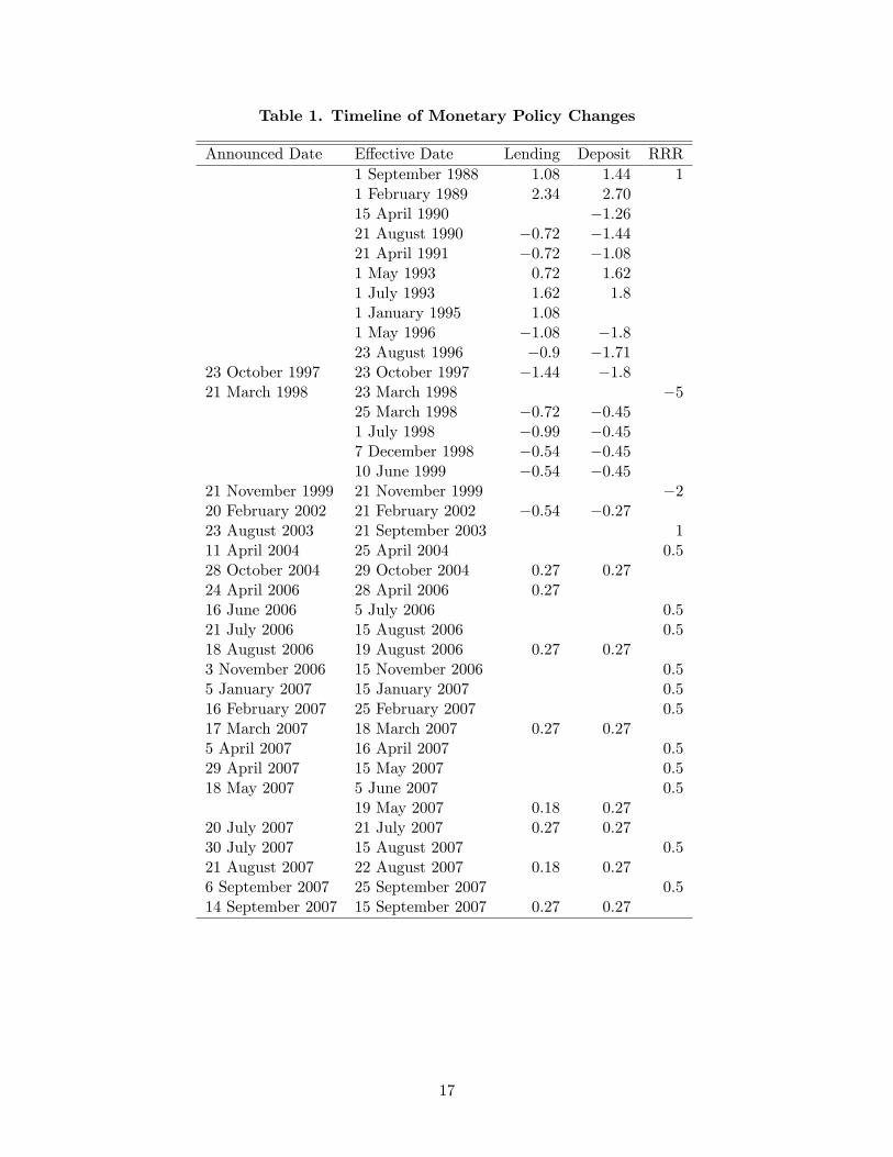
Table 1. Timeline of Monetary Policy Changes

Announced Date Effective Date Lending Deposit RRR1 September 1988 1.08 1.44 11 February 1989 2.34 2.7015 April 1990 −1.2621 August 1990 −0.72 −1.4421 April 1991 −0.72 −1.081 May 1993 0.72 1.621 July 1993 1.62 1.81 January 1995 1.081 May 1996 −1.08 −1.823 August 1996 −0.9 −1.71

23 October 1997 23 October 1997 −1.44 −1.821 March 1998 23 March 1998 −5

25 March 1998 −0.72 −0.451 July 1998 −0.99 −0.457 December 1998 −0.54 −0.4510 June 1999 −0.54 −0.45

21 November 1999 21 November 1999 −220 February 2002 21 February 2002 −0.54 −0.2723 August 2003 21 September 2003 111 April 2004 25 April 2004 0.528 October 2004 29 October 2004 0.27 0.2724 April 2006 28 April 2006 0.2716 June 2006 5 July 2006 0.521 July 2006 15 August 2006 0.518 August 2006 19 August 2006 0.27 0.273 November 2006 15 November 2006 0.55 January 2007 15 January 2007 0.516 February 2007 25 February 2007 0.517 March 2007 18 March 2007 0.27 0.275 April 2007 16 April 2007 0.529 April 2007 15 May 2007 0.518 May 2007 5 June 2007 0.5

19 May 2007 0.18 0.2720 July 2007 21 July 2007 0.27 0.2730 July 2007 15 August 2007 0.521 August 2007 22 August 2007 0.18 0.276 September 2007 25 September 2007 0.514 September 2007 15 September 2007 0.27 0.27

17

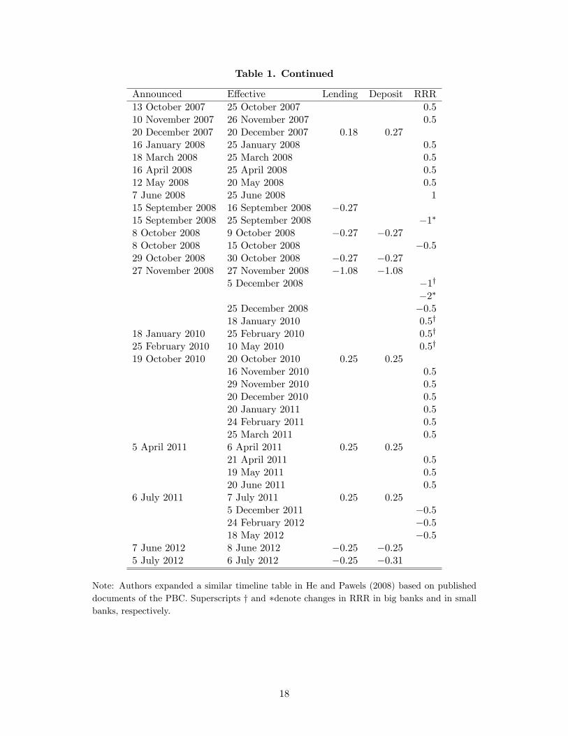
Table 1. Continued

Announced Effective Lending Deposit RRR13 October 2007 25 October 2007 0.510 November 2007 26 November 2007 0.520 December 2007 20 December 2007 0.18 0.2716 January 2008 25 January 2008 0.518 March 2008 25 March 2008 0.516 April 2008 25 April 2008 0.512 May 2008 20 May 2008 0.57 June 2008 25 June 2008 115 September 2008 16 September 2008 −0.2715 September 2008 25 September 2008 −1∗

8 October 2008 9 October 2008 −0.27 −0.278 October 2008 15 October 2008 −0.529 October 2008 30 October 2008 −0.27 −0.2727 November 2008 27 November 2008 −1.08 −1.08

5 December 2008 −1†

−2∗

25 December 2008 −0.518 January 2010 0.5†

18 January 2010 25 February 2010 0.5†

25 February 2010 10 May 2010 0.5†

19 October 2010 20 October 2010 0.25 0.2516 November 2010 0.529 November 2010 0.520 December 2010 0.520 January 2011 0.524 February 2011 0.525 March 2011 0.5

5 April 2011 6 April 2011 0.25 0.2521 April 2011 0.519 May 2011 0.520 June 2011 0.5

6 July 2011 7 July 2011 0.25 0.255 December 2011 −0.524 February 2012 −0.518 May 2012 −0.5

7 June 2012 8 June 2012 −0.25 −0.255 July 2012 6 July 2012 −0.25 −0.31

Note: Authors expanded a similar timeline table in He and Pawels (2008) based on publisheddocuments of the PBC. Superscripts † and ∗denote changes in RRR in big banks and in smallbanks, respectively.

18

Table 2. Augmented Dickey-Fuller Test Results

ADFc ADFtiLt −1.308 −2.721iDt −1.162 −1.974πt −3.845‡ −4.170‡

yQt −3.366† −3.363∗

yHt −4.313‡ −4.305‡

∆mt −4.149‡ −4.459‡

∆st −9.404‡ −9.594‡

Note: ADFcand ADFtdenote the augmented Dickey-Fuller unit root test statistics when anintercept is included and when both an intercept and time trend are present, respectively. Weselect the number of lags by the general-to-specific rule with a maximum 12 lags and the 10%significance level. *, †, and ‡denote rejections of the unit root null hypothesis at the 10%, 5%,and 1% significance level, respectively.

19

Table 3. Linear Taylor Rule Coeffi cient Estimations

(a) Lending RatesLong-Run Coeffi cients

πt−1 0.166(0.024) 0.165(0.025) 0.171(0.027) 0.171(0.028)yt−1 −0.004(0.026) −0.003(0.027) −0.008(0.028) −0.008(0.029)∆mt−1 n.a. 0.002(0.016) n.a. 0.002(0.016)∆st−1 n.a. n.a. 0.004(0.009) 0.004(0.009)

Short-Run Coeffi cients with Interest Rate Smoothingπt−1 0.037(0.007) 0.036(0.007) −0.038(0.008) −0.037(0.008)yt−1 −0.002(0.007) −0.001(0.007) −0.003(0.007) −0.002(0.007)∆mt−1 n.a. 0.001(0.004) n.a. 0.001(0.004)∆st−1 n.a. n.a. 0.001(0.002) 0.001(0.002)it−1 0.904(0.023) 0.903(0.023) 0.903(0.023) 0.903(0.023)

(b) Deposit RatesLong-Run Coeffi cients

πt−1 0.268(0.033) 0.264(0.043) 0.265(0.035) 0.262(0.036)yt−1 0.009(0.018) 0.011(0.018) 0.001(0.018) 0.011(0.019)∆mt−1 n.a. 0.015(0.023) n.a. 0.015(0.023)∆st−1 n.a. n.a. −0.002(0.013) −0.002(0.013)

Short-Run Coeffi cients with Interest Rate Smoothingπt−1 0.046(0.008) 0.045(0.008) 0.049(0.009) 0.048(0.009)yt−1 −0.004(0.004) −0.004(0.004) −0.006(0.004) −0.005(0.004)∆mt−1 n.a. 0.007(0.005) n.a. 0.008(0.005)∆st−1 n.a. n.a. 0.004(0.003) 0.004(0.003)it−1 0.923(0.020) 0.922(0.019) 0.924(0.019) 0.923(0.019)

Note: Standard errors are in parenthesis. Output gap is the HP cyclical component. Using thequadratically detrended gap yields qualitatively similar results. All results are available uponrequest.

20

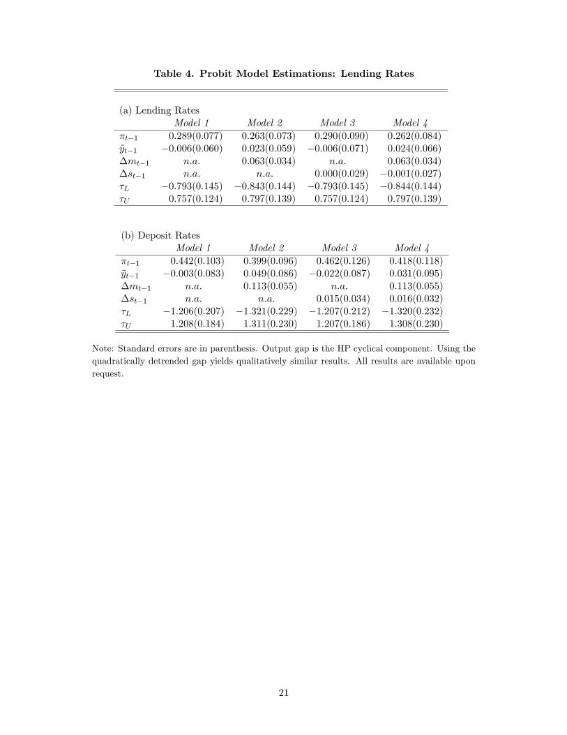
Table 4. Probit Model Estimations: Lending Rates

(a) Lending RatesModel 1 Model 2 Model 3 Model 4

πt−1 0.289(0.077) 0.263(0.073) 0.290(0.090) 0.262(0.084)yt−1 −0.006(0.060) 0.023(0.059) −0.006(0.071) 0.024(0.066)∆mt−1 n.a. 0.063(0.034) n.a. 0.063(0.034)∆st−1 n.a. n.a. 0.000(0.029) −0.001(0.027)τL −0.793(0.145) −0.843(0.144) −0.793(0.145) −0.844(0.144)τU 0.757(0.124) 0.797(0.139) 0.757(0.124) 0.797(0.139)

(b) Deposit RatesModel 1 Model 2 Model 3 Model 4

πt−1 0.442(0.103) 0.399(0.096) 0.462(0.126) 0.418(0.118)yt−1 −0.003(0.083) 0.049(0.086) −0.022(0.087) 0.031(0.095)∆mt−1 n.a. 0.113(0.055) n.a. 0.113(0.055)∆st−1 n.a. n.a. 0.015(0.034) 0.016(0.032)τL −1.206(0.207) −1.321(0.229) −1.207(0.212) −1.320(0.232)τU 1.208(0.184) 1.311(0.230) 1.207(0.186) 1.308(0.230)

Note: Standard errors are in parenthesis. Output gap is the HP cyclical component. Using thequadratically detrended gap yields qualitatively similar results. All results are available uponrequest.

21

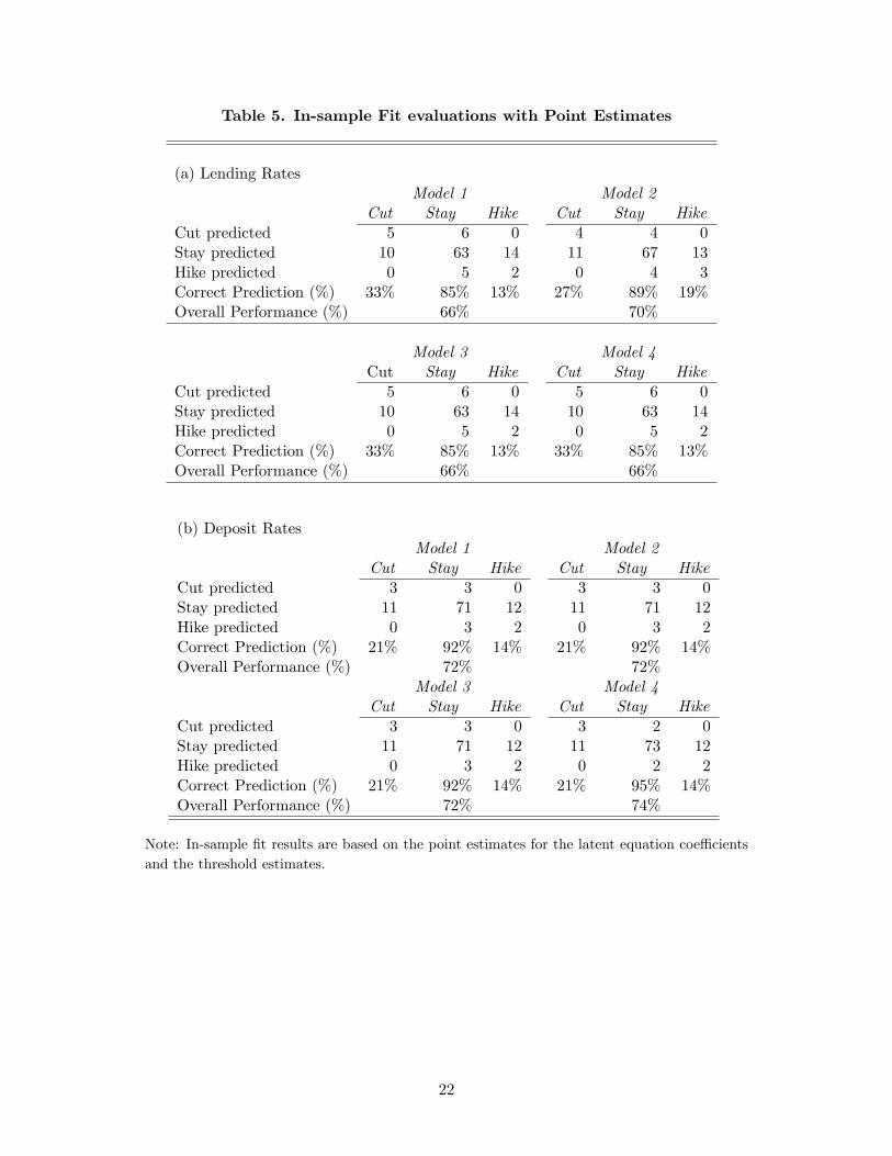
Table 5. In-sample Fit evaluations with Point Estimates

(a) Lending RatesModel 1 Model 2

Cut Stay Hike Cut Stay HikeCut predicted 5 6 0 4 4 0Stay predicted 10 63 14 11 67 13Hike predicted 0 5 2 0 4 3Correct Prediction (%) 33% 85% 13% 27% 89% 19%Overall Performance (%) 66% 70%

Model 3 Model 4Cut Stay Hike Cut Stay Hike

Cut predicted 5 6 0 5 6 0Stay predicted 10 63 14 10 63 14Hike predicted 0 5 2 0 5 2Correct Prediction (%) 33% 85% 13% 33% 85% 13%Overall Performance (%) 66% 66%

(b) Deposit RatesModel 1 Model 2




Note: In-sample fit results are based on the point estimates for the latent equation coeffi cientsand the threshold estimates.

22

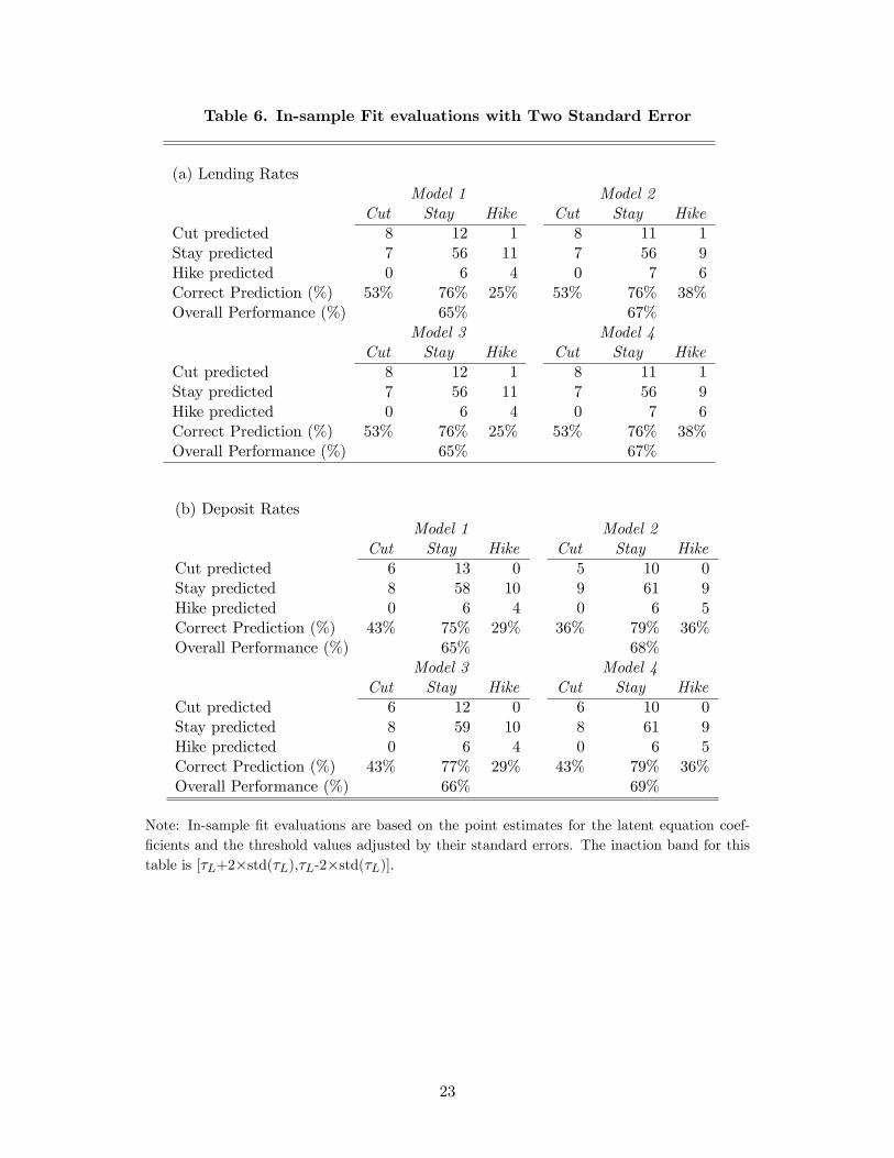
Table 6. In-sample Fit evaluations with Two Standard Error

(a) Lending RatesModel 1 Model 2




(b) Deposit RatesModel 1 Model 2




Note: In-sample fit evaluations are based on the point estimates for the latent equation coef-ficients and the threshold values adjusted by their standard errors. The inaction band for thistable is [τL+2×std(τL),τL-2×std(τL)].

23

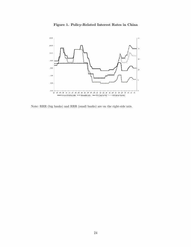
Figure 1. Policy-Related Interest Rates in China

Note: RRR (big banks) and RRR (small banks) are on the right-side axis.

24

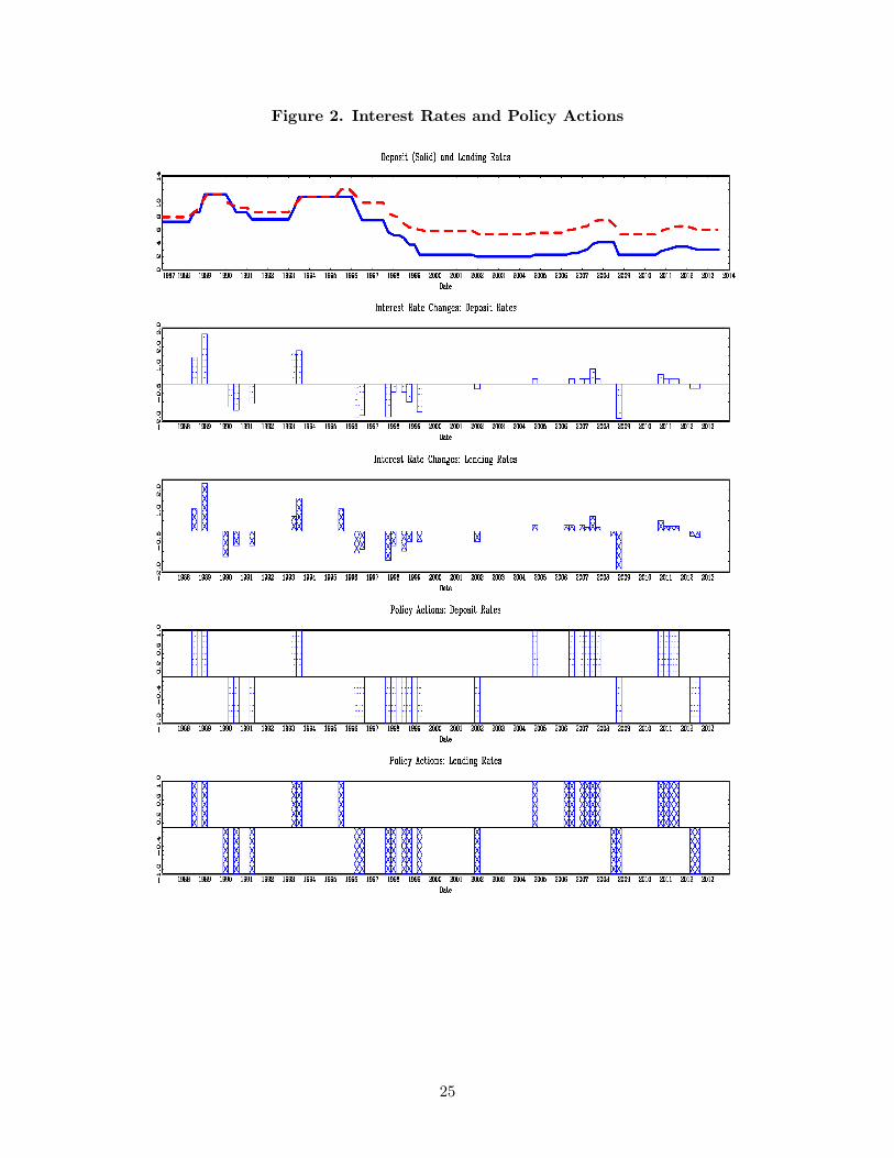
Figure 2. Interest Rates and Policy Actions

25

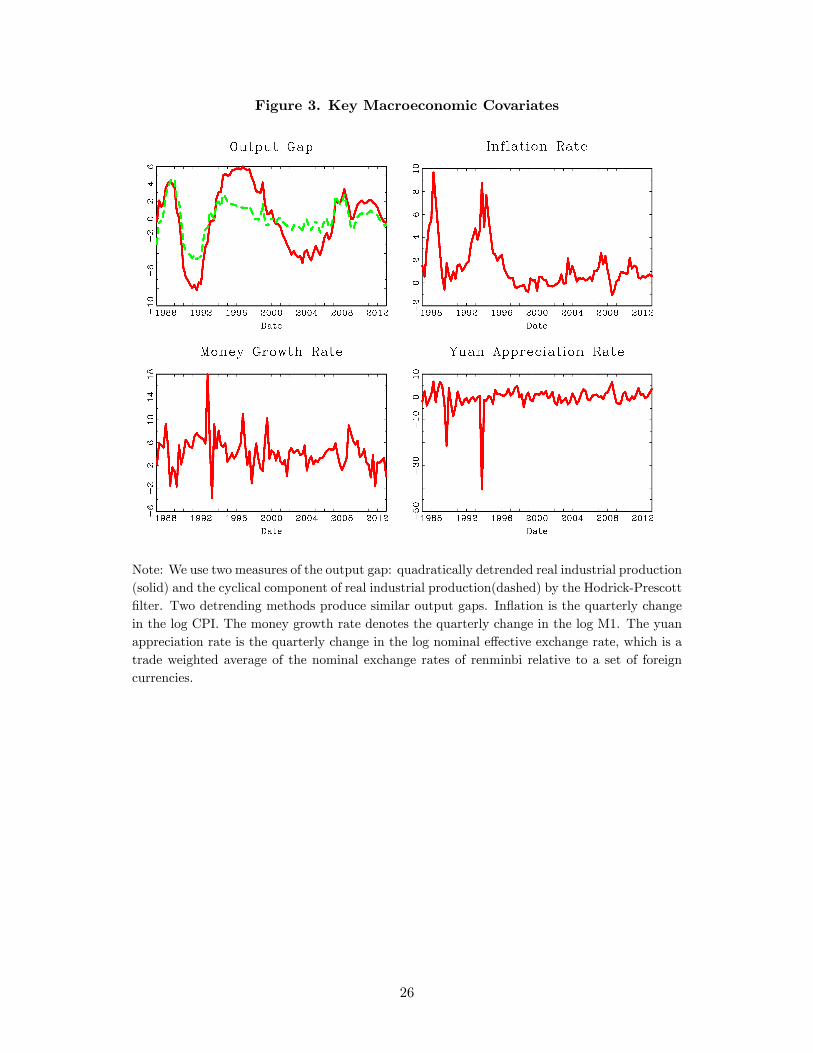
Figure 3. Key Macroeconomic Covariates

Note: We use two measures of the output gap: quadratically detrended real industrial production(solid) and the cyclical component of real industrial production(dashed) by the Hodrick-Prescottfilter. Two detrending methods produce similar output gaps. Inflation is the quarterly changein the log CPI. The money growth rate denotes the quarterly change in the log M1. The yuanappreciation rate is the quarterly change in the log nominal effective exchange rate, which is atrade weighted average of the nominal exchange rates of renminbi relative to a set of foreigncurrencies.

26

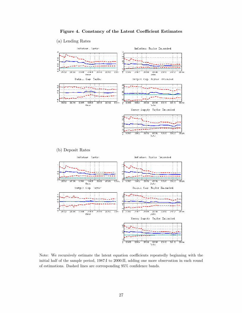
Figure 4. Constancy of the Latent Coeffi cient Estimates

(a) Lending Rates

(b) Deposit Rates

Note: We recursively estimate the latent equation coeffi cients repeatedly beginning with theinitial half of the sample period, 1987:I to 2000:II, adding one more observation in each roundof estimations. Dashed lines are corresponding 95% confidence bands.

27

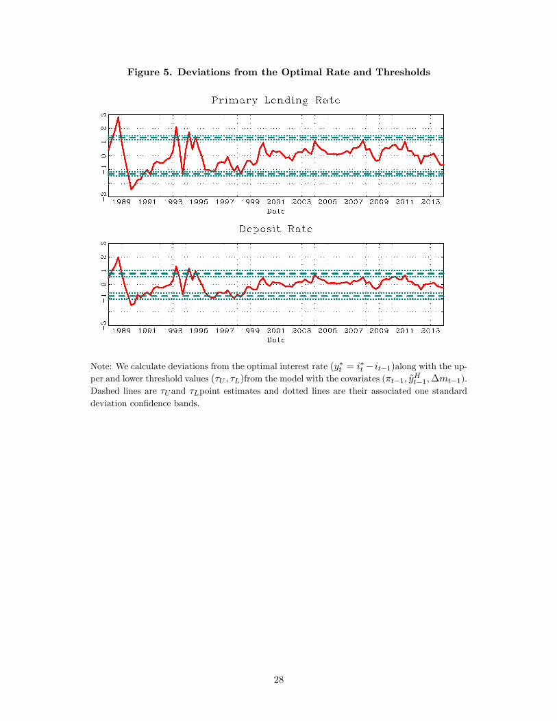
Figure 5. Deviations from the Optimal Rate and Thresholds

Note: We calculate deviations from the optimal interest rate (y∗t = i∗t − it−1)along with the up-per and lower threshold values (τU , τL)from the model with the covariates (πt−1, yHt−1,∆mt−1).Dashed lines are τUand τLpoint estimates and dotted lines are their associated one standarddeviation confidence bands.

28

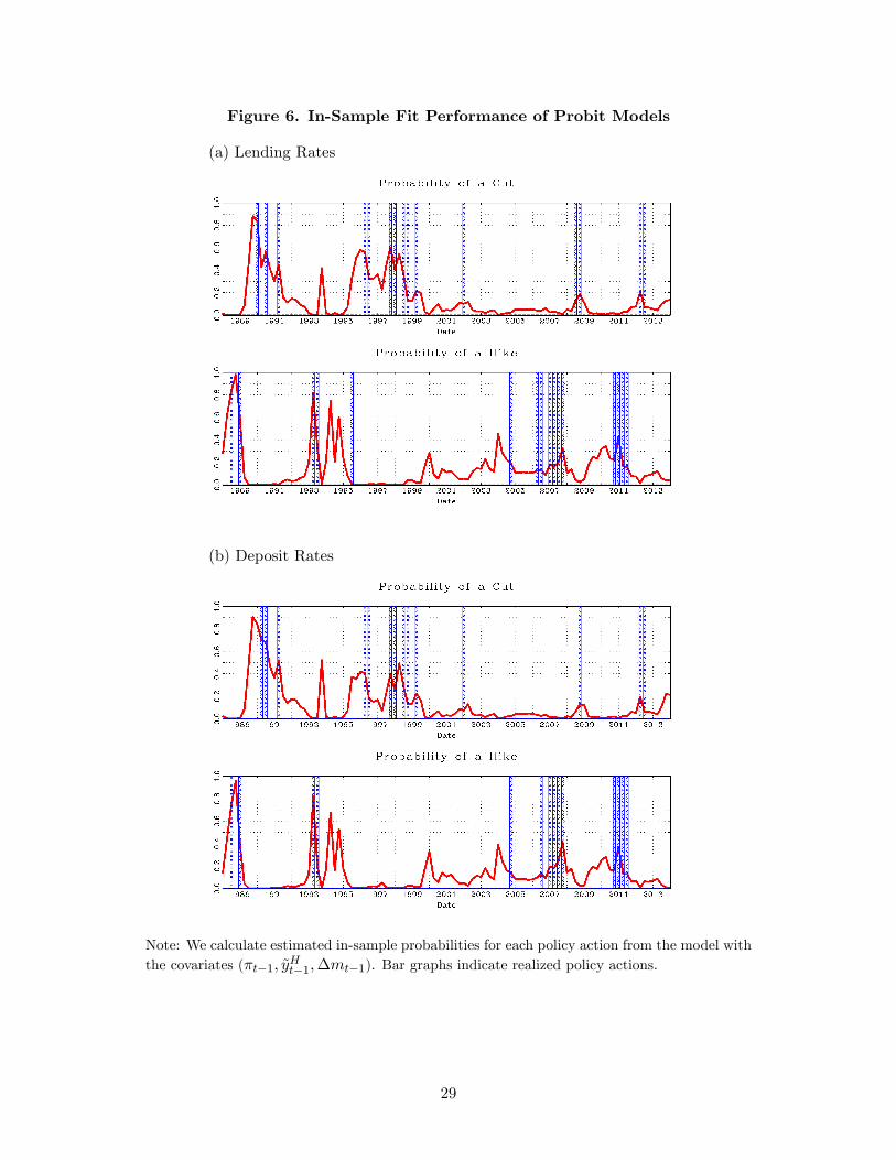
Figure 6. In-Sample Fit Performance of Probit Models

(a) Lending Rates

(b) Deposit Rates

Note: We calculate estimated in-sample probabilities for each policy action from the model withthe covariates (πt−1, yHt−1,∆mt−1). Bar graphs indicate realized policy actions.

29

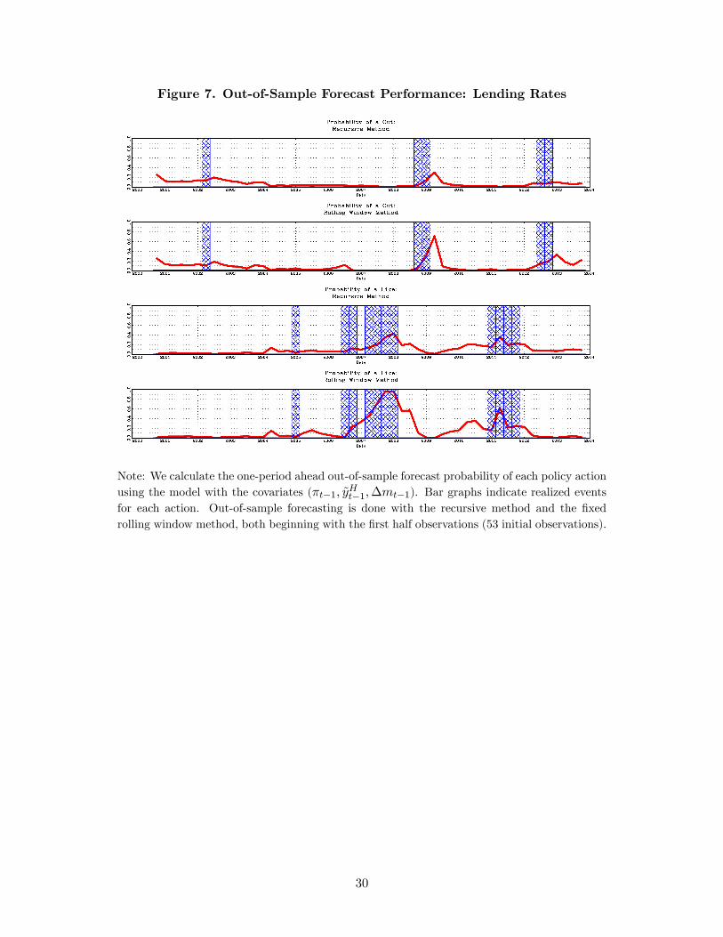
Figure 7. Out-of-Sample Forecast Performance: Lending Rates

Note: We calculate the one-period ahead out-of-sample forecast probability of each policy actionusing the model with the covariates (πt−1, yHt−1,∆mt−1). Bar graphs indicate realized eventsfor each action. Out-of-sample forecasting is done with the recursive method and the fixedrolling window method, both beginning with the first half observations (53 initial observations).

30

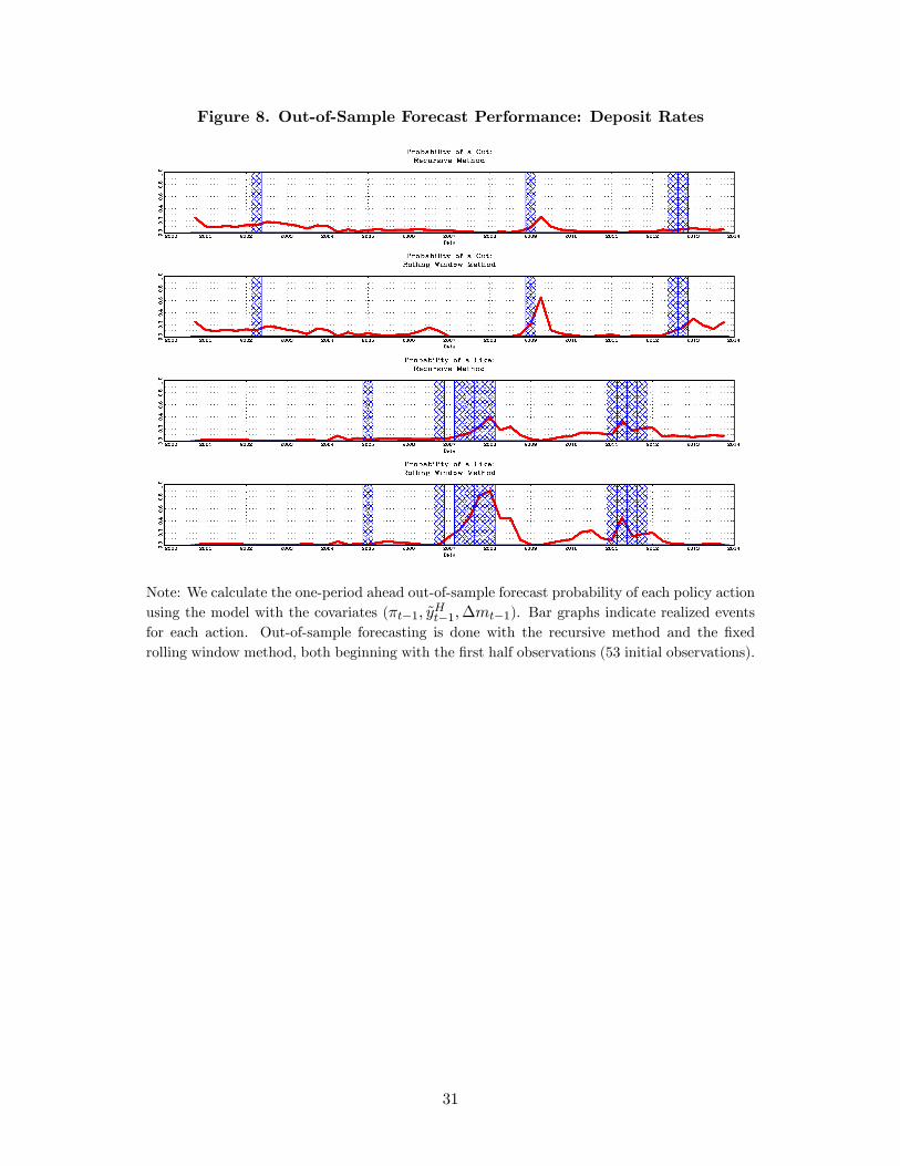
Figure 8. Out-of-Sample Forecast Performance: Deposit Rates

Note: We calculate the one-period ahead out-of-sample forecast probability of each policy actionusing the model with the covariates (πt−1, yHt−1,∆mt−1). Bar graphs indicate realized eventsfor each action. Out-of-sample forecasting is done with the recursive method and the fixedrolling window method, both beginning with the first half observations (53 initial observations).

31

The Determinants of the Benchmark Interest Rates in China: A Discrete Choice Model Approach

Documents

Transcript of The Determinants of the Benchmark Interest Rates in China: A Discrete Choice Model Approach