A Tool to Evaluate the Safety Effects of Changes in Freeway Traffic Flow

eScholarship provides open access, scholarly publishingservices to the University of California and delivers a dynamicresearch platform to scholars worldwide.

California Partners for AdvancedTransportation Technology

UC Berkeley

Title:A Tool to Evaluate the Safety Effects of Changes in Freeway Traffic Flow

Author:Golob, Thomas F.Recker, Wilfred W.Alvarez, Veronica M.

Publication Date:06-01-2003

Series:Working Papers

Permalink:http://escholarship.org/uc/item/1kn30323

Abstract:This research involves the development of a tool that can be used to assess the changes in trafficsafety tendencies that result from changes in traffic flow. The tool uses data from single inductiveloop detectors, converting 30-second observations of volume and occupancy for multiple freewaylanes into traffic flow regimes. Each regime has a specific pattern of crash types, which weredetermined through nonlinear multivariate analyses of over 1,000 crashes on freeways in SouthernCalifornia. These analyses revealed ways in which differences in variances in speeds and volumesacross lanes, as well as central tendencies of speeds and volumes, combine in complex ways toexplain crash taxonomy. This research may provide the foundation to forecast the crash rates, interms of vehicle miles of travel, for vehicles that are exposed to different traffic flow conditions.

Copyright Information:All rights reserved unless otherwise indicated. Contact the author or original publisher for anynecessary permissions. eScholarship is not the copyright owner for deposited works. Learn moreat http://www.escholarship.org/help_copyright.html#reuse

http://escholarship.org




http://escholarship.org/uc/its_path_papers



http://escholarship.org/uc/ucb

http://escholarship.org/uc/search?creator=Golob%2C%20Thomas%20F.

http://escholarship.org/uc/search?creator=Recker%2C%20Wilfred%20W.

http://escholarship.org/uc/search?creator=Alvarez%2C%20Veronica%20M.


http://escholarship.org/uc/item/1kn30323

http://www.escholarship.org/help_copyright.html#reuse

CALIFORNIA PATH PROGRAMINSTITUTE OF TRANSPORTATION STUDIESUNIVERSITY OF CALIFORNIA, BERKELEY

This work was performed as part of the California PATH Program of the University of California, in cooperation with the State of California Business, Transportation, and Housing Agency, Department of Trans-portation; and the United States Department Transportation, Federal Highway Administration.

The contents of this report reflect the views of the authors who are responsible for the facts and the accuracy of the data presented herein. The contents do not necessarily reflect the official views or policies of the State of California. This report does not constitute a standard, spec-ification, or regulation.

ISSN 1055-1417

June 2003

A Tool to Evaluate the Safety Effects of Changes in Freeway Traffic Flow

California PATH Working PaperUCB-ITS-PWP-2003-9

CALIFORNIA PARTNERS FOR ADVANCED TRANSIT AND HIGHWAYS

Thomas F. Golob, Wilfred W. Recker, Veronica M. AlvarezUniversity of California, Irvine

Report for Task Order 4117

A Tool to Evaluate the Safety Effects of Changes in Freeway Traffic Flow Thomas F. Golob Institute of Transportation Studies University of California, Irvine +1.949.824.6287 [email protected]

Wilfred W. Recker Department of Civil and Environmental Engineering and Institute of Transportation Studies University of California, Irvine +1.949.824.5642 [email protected]

Veronica M. Alvarez Institute of Transportation Studies University of California, Irvine +1.949.824.6571 [email protected] April 30, 2003 To appear in

Journal of Transportation Engineering (ASCE)

A Tool to Evaluate the Safety Effects of Changes in Freeway Traffic Flow by Thomas F. Golob, Wilfred W. Recker, and Veronica M. Alvarez

Abstract

This research involves the development of a tool that can be used to assess the changes in traffic safety tendencies that result from changes in traffic flow. The tool uses data from single inductive loop detectors, converting 30-second observations of volume and occupancy for multiple freeway lanes into traffic flow regimes. Each regime has a specific pattern of crash types, which were determined through nonlinear multivariate analyses of over 1,000 crashes on freeways in Southern California. These analyses revealed ways in which differences in variances in speeds and volumes across lanes, as well as central tendencies of speeds and volumes, combine in complex ways to explain crash taxonomy. This research may provide the foundation to forecast the crash rates, in terms of vehicle miles of travel, for vehicles that are exposed to different traffic flow conditions. An earlier version of this paper was presented at the 82nd Annual Meeting of the Transportation Research Board, Washington, DC, January 12-26, 2003

Golob Recker Alvarez A Tool to Evaluate the Safety Effects of Changes in Freeway Traffic Flow 1

1 Background Benefit/cost comparisons have long been a standard in assessing the effectiveness of investment of limited resources, and have served as an essential element in determining the most effective allocation of such resources. Assessment of benefits of ATMS and ITS improvements largely translates into a problem of quantifying the benefits of improved traffic flow. Improved flow ostensibly leads to reductions in travel time, vehicle emissions, fuel usage, psychological stress on drivers, and improved safety. Developing these comparisons presents a perplexing problem for operating agencies, primarily because hard numbers cannot be obtained practically by direct measurement (e.g., by shutting down ramp metering or curtailing freeway service patrols for a period of time to measure consequences). This measurement problem is heightened dramatically when issues of safety are involved, but one of the most compelling arguments for implementation of ITS elements is their presumed enhancement of traffic safety. There is strong empirical evidence of functional relationships between crash rates and traffic flow (Aljanahi, et al., 1999, Cedar and Livneh, 1982, Dickerson, Peirson and Vickerman, 2000, Frantzeskakis and Iordanis, 1987, Garber and Gadiraju, 1990, Gwynn, 1967, Hall and Pendleton, 1989, Jansson, 1994, Johansson, 1996, Jones-Lee, 1990, Maher and Summersgill, 1996, Newberry, 1988, O’Reilly, et al., 1994, Sandhu and Al-Kazily, 1996, Shefer and Rietveld, 1997, Stokes and Mutabazi, 1996, Sullivan, 1990, Sullivan and Hsu, 1988, Vickery, 1969, Vitaliano and Held, 1991, and Zhou and Sisiopiku, 1997). Nevertheless, the manner in which safety is improved by smoothing traffic flow is not well understood at this time. The present research is aimed at shedding light on the complex relationships between traffic flow and traffic crashes. The overall objective is to develop an evaluation tool that uses relationships between traffic flow and crash characteristics to assess the safety benefits that are likely to be realized under specific ATMS implementations. A software tool, called FITS (Flow Impacts on Traffic Safety) has been developed that uses a data stream of 30-second observations from single inductance loop detectors to forecast the types of crashes that are most likely to occur for the flow conditions being monitored. The algorithm, in its present form, is based on analyses of crash characteristics of more than 1,000 crashes on six major freeways Orange County California in 1998 as a function of traffic flow conditions for a thirty-minute time period immediately preceding the crashes. The algorithm could be re-estimated for other urban areas if similar data were available. In previous research (Golob and Recker, 2002), we conducted a series of analyses aimed at determining the extent to which traffic flow variables, in the form of 30-second observations from single inductive loop detectors, account for variation in accident typology, controlling for ambient weather (wet or dry) and lighting (daylight or nighttime) conditions. The data used here, as described in Section 2, are a subset of the data used in the previous study. In the previous study we used nonlinear (nonparametric) canonical correlation analysis applied with three sets of variables: crash characteristics, traffic flow variables, and segmentation based on weather and lighting conditions.


Nonlinear canonical correlation analysis (NLCCA) (Gifi, 1990, de Leeuw, 1985, Michailidis and de Leeuw, 1998, van de Geer, 1986, ver Boon, 1996, van der Burg and de Leeuw, 1983) is a form of canonical correlation analysis in which categorical and ordinal variables are optimally scaled as an integral component in finding linear combinations of variables with the highest correlations among them. The analysis revealed clear patterns relating crash characteristics and prevailing traffic flow conditions, and it showed how these relationships are conditional upon lighting and weather. Prevailing traffic flow conditions were measured in terms of statistics derived from approximately 30 minutes of lane-specific 30-second loop-detector observations prior to the time of each crash. We concluded from the Golob and Recker (2002) study that an evaluation tool could be developed to forecast the types of crashes that are most likely to occur under different traffic flow conditions. This tool uses a similar data stream of observations from single inductive loop detectors and is based on some of the same statistical methods used in the previous study, with the addition of several new steps required for monitoring and forecasting purposes. Our results may provide the foundation to forecast the crash rates, in terms of vehicle miles of travel, for vehicles that are exposed to different traffic flow conditions. The remainder of this paper is organized as follows. Data are discussed in Section 2. In Section 3 we present results of the analyses in which we determine how traffic flow is related to differences in safety. For reporting purposes, results are shown for only one segment of weather and lighting conditions: dry roadways during daylight and dusk-dawn conditions. In Section 4, we apply the tool in a case study of a section of one freeway for one week. In Section 5, we present a hypothetical example of how the FITS tool could be used to assess expected safety benefits accrued from ATMS applications. We close with conclusions and a discussion of future research in Section 6. 2 Data

2.1 Case Study

Our data cover crashes that occurred on six major freeway routes in Orange County California during calendar year 1998. Orange County is located on the Pacific coast between Los Angeles and San Diego Counties, and the six freeways included in this study account for over 209 route kilometers (130 miles), with between 3 and 6 lanes in each direction. Crash data were drawn from the Traffic Accident Surveillance and Analysis System (TASAS) database (Caltrans, 1993), which covers all police-reported crashes on the California State Highway System. In 1998 there were a total of 9,341 mainline crashes on the six Orange County freeway routes. Out of these 9,341 crashes, 1,192 (12.8%) had valid loop detector data for a full 30 minutes preceding the crash for three designated lanes at a loop detector station that was relatively close to the crash. For


each of the crash characteristics used in this study (described in Section 2.3), contingency table chi-squared tests revealed that there is no statistically significant difference (at the 95% confidence level) between the selected subset of 1,192 crashes and the unused subset of 8,150 crashes. The average distance from the crash location to the closest detector station for the 1,192 crashes is 274 meters (0.17 miles) and the median distance is 193 meters (0.12 miles). Fully 78% of these crashes were located within 400 meters (0.25 miles) of the closest detector station. Traffic flow data are in the form of 30-second loop detector data at the closet detector station to the scene of the crash for 30 minutes preceding the reported time of the crash. Each observation provides count and percentage occupancy for a 30-second time slice. At each mainline loop detector station, data are available for each freeway lane. A consistent scheme was used for designation of lanes comprising the analysis: (a) the left lane, always being the lane designated as being the number one lane according to standard nomenclature; (b) one interior lane, being lane number two on three- and four-lane freeway sections and lane number three on five- and six-lane sections; and (c) the right lane. Because the reported times are typically rounded off to five-minute intervals, crash times are not know with precision. In recognition of this, the loop data for the 2.5-minute period immediately preceding the reported times were discarded in order to avoid potential inclusion of post-crash conditions. 2.2 Segmentation Based on Weather and Lighting Conditions

In Golob and Recker (2002), we present empirical evidence confirming previous observations (e.g., Fridstrøm, et al., 1995) that relationships between safety and traffic flow conditions depend upon driving conditions defined, by weather and ambient lighting conditions. By analyzing all combinations of lighting and weather conditions, we determined that the Wet-Night and Wet-Day segments can be combined into a single Wet segment, and the relatively sparse Dry-Dusk-Dawn segment can be combined with the Dry-Day segment. The resulting segmentation for Orange County crashes in 1998 is: (1) Dry-Day (including Dusk-Dawn): 819 crashes, (2) Dry-Night, 217 crashes, and (3) Wet (any lighting condition): 156 crashes. For the purpose of developing an evaluation tool, we conducted separate analyses for each of these three segments. However, for purposes of brevity, in the remainder of this paper we report on results for only the largest segment: daylight and dusk-dawn conditions on dry roads.

2.3 Crash Characteristics

Three crash characteristics were used in this analysis: (1) crash type, based on the type of collision (rear end, sideswipe, or hit object), the number of vehicles involved, and the movement of these vehicles prior to the crash, (2) the crash location, based on the location of the primary collision (e.g., left lane, interior lanes, right lane, right shoulder area, off-road beyond right shoulder area), and (3) crash severity, in terms injuries and fatalities per vehicle. Based on exploratory statistical analyses, and taking into account requirements on minimum category frequencies, we used six categories of crash type,


five categories of crash location, and two categories of crash severity. We were only able to use two categories for crash severity because there were very few fatal crashes and the extent of non-fatal injuries is not recorded in the TASAS database. These variables are described in Table 1.

Table 1 Characteristics of Crashes during Daylight on Dry Roads (N = 819 crashes)

Crash Characteristic Percent of sample

Crash type Single vehicle hit object or overturn 10.5 Multiple vehicle hit object or overturn 5.6 2-vehicle weaving crash a 17.8 3-or-more-vehicle weaving crash a 5.1 2-vehicle straight-on rear end crash 38.2 3-or-more-vehicle straight-on rear end 22.7

Crash Location Off-road, driver’s left 12.3 Left lane 30.4 Interior lane(s) 32.5 Right lane 18.7 Off road, driver’s right 6.1

Severity Property damage only 75.0 Injury or fatality 25.0

a Sideswipe or rear end crash involving lane change or other turning maneuver

2.4 Traffic Flow Variables

This research uses raw detector data that provide information on two variables: count and occupancy for each thirty-second interval. Although these two variables can be used (under very restrictive assumptions of uniform speed and average vehicle length, and taking into account the physical installation of each loop) to infer estimates of point speeds, we avoid making any such assumptions, and use only these direct measurements. Based on preliminary analyses, four blocks of three variables (one variable for each of the three lanes: left, interior, and right) were found to be related to crash typology. (1) The first block comprises the median of the ratio of volume to occupancy for each of the three lanes, and measures the central tendency of (density), an approximate proportional indicator of space mean speed. Median, rather than mean, is used in order to avoid the influence of outlying observations that can be due to failure of the loop


detectors or unusual vehicle mixes. (2) The second block comprises the difference of the 90th percentile and 50th percentile in the ratio of volume to occupancy (density) for each lane, and represents the temporal variation of this ratio. Here we use the percentile differences because we wish to minimize the influence of outlying observations. (3) The third block comprises the mean volumes for all three lanes taken over the entire 27.5-minute period preceding the accident. Volume alone is not as sensitive to outliers as the ratio of volume to occupancy is, so mean, rather than median, is used as a measure of central tendency. (4) Finally, the fourth block is composed of the standard deviations of the 30-second volumes for all three lanes as a measure of variation in volume over the 27.5-minute period. We expect that some of the traffic flow variables will be highly correlated, clouding interpretation of analysis results. Specifically, the three variables in each of the four blocks might be highly correlated if the flow characteristic being measured is consistent across all three lanes. However, it is not known how strongly these particular measures of traffic flow are linked across lanes, and this is especially true of speed and volume variances. To minimize this potential problem, we apply principal components analysis (PCA) to extract a sufficient number of factors to identify independent traffic flow variables while simultaneously discarding as little of the information in the original variables as possible. A PCA with varimax rotation was performed on the twelve traffic flow variables (i.e., the four blocks of three variables defined above) for the group of crashes that occurred during daylight or dusk-dawn on dry roads. Six factors accounted for 86.8% of the variance in the original twelve variables. One variable was then selected to represent each factor in the subsequent stages of the analysis. These six variables are listed in Table 2, together with the factor that they represent.

Table 2 Loop Detector Variables Used to as Input to the FITS Tool

Specific Variable Factor Represented

Median volume/occupancy interior lane Central tendency of speed - all lanes

90th%tile - 50th%tile of volume/occupancy interior lane Variation in speed – all but right lane

90th%tile - 50th%tile of volume/occupancy right lane Variation in speed – right lane

Mean volume left lane Central tendency of volume - all lanes

Standard deviation of volume interior lane Variation in volume – all but right lane

Standard deviation of volume right lane Variation in volume – right lane

The factor loadings (not shown) indicate that the central tendency of speed (Variable Block 1) is consistent across all three lanes. The variable chosen to represent this central tendency of speed factor is median volume/occupancy in the interior lane. The


second factor represents the temporal variation in volume/density on the left and interior lanes only. Variation in volume/density in the right lane is captured by a separate, third, factor. The implication here is that the variation in speed in the rightmost lane, which tends to be influenced by weaving in the vicinity of freeway on- and off-ramps, relates to crash characteristics in a fundamentally different way than does the variation in speed that is attributable primarily to mainline freeway flow. A single factor (the fourth factor in Table 2) also encompasses the central tendency of volume in all three lanes. Mean volume in the left lane was chosen to represent this factor in all further analyses. Finally, the PCA results also show that temporal variations in volumes on the three lanes is partitioned into two factors: variations in volume on the left and interior lanes (fifth factor), and variation in volume on the right lane (sixth and last factor in Table 2). Volume in the rightmost lane, which has a direct influence on the level of service in the vicinity of freeway on- and off-ramps, relates to crash characteristics in a fundamentally different way than does flow in the other lanes. 3 Finding Traffic Flow Regimes that Best Explain Crash Typology

3.1 Clustering in the Six-dimensional Space of the Traffic Flow Variables

Cluster analyses were performed in the space of these six principal traffic flow variables in order to establish relatively homogenous traffic flow regimes. A k-means clustering algorithm was used. The objective was to determine the best grouping of observations into a specified number of clusters, such that the pooled within groups variance is as small as possible compared to the between group variance given by the distances between the cluster centers. We repeated runs of the clustering algorithm with different initial cluster centers to avoid local optima. The optimal number of clusters, specific to any particular problem, is usually determined by inspecting clustering criteria developed from eigenvalues of the characteristic equation involving the ratio of the pooled within-groups and between-groups covariance matrices (e.g., Wilk’s Lambda, given by the ratio of the determinants of the within-groups and total covariance matrices, or Hotelling’s Trace, given by the sum of the eigenvalues of the characteristic equation). Selection of the optimal number of groups using such criteria is relatively arbitrary. To reduce such arbitrariness, we instead conducted a nonlinear canonical correlation analysis (NLCCA, described in Section 1) for each clustering solution, adopting a two-dimensional solution. The NLCCA problem was configured with the multiple nominal cluster variable on one side and the three single nominal crash variables described in Table 1 on the other side. The criteria that describe how well each of the cluster variables explained the crash characteristics are the canonical correlations between the two sets of variables, one for each of the variates of the two-dimensional solution. For prevailing traffic conditions for crashes on dry roads during daylight, the canonical correlations for the first dimension were found to reach a maximum at eight clusters; the fit for the second dimension has a local maximum at eight clusters, but does not achieve a global optimum until the 13-cluster


level is reached. Based on these results, and corroborative evidence from Wilk’s Lambda and Hotelling’s Trace, we selected eight clusters, which we refer to as eight distinct Traffic Flow Regimes. The eight traffic flow regimes can be described based on the location of their cluster centers in the six-dimensional space of the traffic flow variables. Briefly, they are, ordered in terms of increasing flow: (D1) light free flow, (D2) heavily congested flow, (D3) congested flow, (D4) light right-variable flow, (D5) flow at capacity, (D6) heavy, variable flow, (D7) heavy, steady flow, and (D8) flow near capacity. A more complete description is provided in Table 4 below.

3.2 Crash Profiles for Eight Traffic Flow Regimes

Nonlinear canonical correlation analysis (NLCCA) of the eight-category regime segmentation variable versus the three crash characteristics was used to determine how the traffic flow regimes are related to patterns of crash characteristics. Another way to view the problem is to ask how the crash characteristics distinguish among traffic flow regimes. Indeed, NLCCA with a single categorical (segmentation) variable in one set is equivalent to nonlinear (nonparametric) discriminant analysis. A two-dimensional NLCCA solution was chosen. The canonical correlations, which indicate the percentage of variance which is shared between the two sets of variables – (1) the traffic flow regimes and (2) the crash characteristics – are 0.424 for the first canonical variate and 0.150 for the second variate. Thus, the first variate is considerably more important in explaining differences in crash characteristics in terms of traffic flow regimes. The two independent variates combine to explain 0.574 of shared variance between the two sets of variables. The R2 value for the regression of the optimally scaled crash characteristics on each of the independent canonical variates is 0.712 for the first canonical variate and 0.574 for the second variate. Table 3 lists the centroids for all categories of the four optimally scaled variables on the two independent canonical variates. These category centroids can be used to label the canonical variates. The distances between the centroids of any two categories in the two-dimensional space of the canonical variates is a measure of the association between the categories. The traffic flow regimes (Table 3) are ordered on the first variate from low to high in terms of decreasing mean speed in the interior lanes. The four regimes that score in the positive domain of the first variate (D8, D5, D3 and D2) are more similar to one another; they all represent heavy traffic, and their ordering from low to high is according to mean volume, rather than mean speed. The first dimension captures aspects of the density (concentration) dimension of the fundamental diagram of traffic flow versus traffic density (Prigogine and Herman, 1971). The second canonical variate, which by definition is independent of the first in terms of its functional relationships with the two sets of variables, primarily distinguishes high-flow regimes (Regimes D5, D6 and D7),


from low-flow regimes (D2 and D1). This dimension captures the flow dimension of the fundamental diagram.

Table 3 Category Centroids – NLCCA of Traffic Flow Regimes versus Three Crash

Characteristics for Crashes During Daylight on Dry Roads

Variable and Category Variate 1 Variate 2

SET 1: Traffic Flow Regime

D1: light free flow -0.87 1.04 D2: heavily congested flow 0.59 1.79 D3: congested flow 0.62 0.24 D4: light right-variable flow -1.74 -0.12 D5: flow at capacity 0.75 -0.87 D6: heavy, variable flow -0.43 -0.46 D7: heavy, steady flow -0.47 -0.36 D8: flow near capacity 0.83 0.25

SET 2: Crash type

Single vehicle hit object or overturn -1.69 -0.37 Multiple vehicle hit object or overturn -1.36 -0.38 2-vehicle weaving crash a -0.24 0.32 3-or-more-vehicle weaving crash a -0.71 -0.19 2-vehicle straight-on rear end 0.54 0.13 3-or-more-vehicle straight-on rear end 0.56 -0.16

SET 2: Crash Location

Off-road, driver’s left -0.71 -0.07 Left lane 0.62 -0.96 Interior lane(s) -0.08 0.72 Right lane 0.10 0.41 Off road, driver’s right -1.50 -0.21

SET 2: Severity Property damage only 0.13 0.15 Injury or fatality -0.39 -0.46

a Sideswipe or rear end crash involving lane change or other turning maneuver

Crash type is more strongly explained by the first (R2=.544) than the second canonical variate (R2=.071). Thus, crash type is related more to density in the fundamental diagram. The optimal scaling of the crash type categories contrasts hit-object versus rear-end crashes, with weaving crashes in between. As expected, rear-end crashes are associated with high density traffic, and hit-object crashes are associated with low density traffic. Weaving crashes (sideswipes and rear-ends caused by lane-change maneuvers) are associated with intermediate density traffic. High-density regimes D8, D3 and D5 are most associated with rear-end crashes, while low-density regimes,


particularly D4, are associated with hit-object crashes. Intermediate-density regimes D6 and D7 are most associated with crashes involving weaving maneuvers. Crash location is more strongly explained by the second canonical variate (R2=.513, versus R2=.049 for the first variate). Crash location is a primarily a flow phenomenon. The optimal scaling of the categories of the location variable shows that left-lane crashes are associated with high density and high flow conditions, while other locations, especially interior lane crashes, are associated with low density and low flow conditions. Regime D5 is especially associated with left lane crashes, while Regime D4 is associated with off-road crashes. Finally, crash severity is explained by both dimensions, on an approximately equal basis. Thus, the difference between property-damage and injury crashes is a function both of flow and density. Injury crashes are more likely to occur in lower density conditions, and in higher flow conditions. Regimes D2 and D4 have the most extreme projections onto the vector defined by the category quantifications of the severity variable. Thus, the NLCCA model predicts that Regime D4 will have a higher proportion of injury crashes, and Regime D2 will have a higher proportion of property-damage-only crashes. The results of the NLCCA model were verified and refined by cross-tabulating each crash characteristic against the eight-category regime segmentation variable. The results were consistent. The traffic flow conditions that define the eight traffic flow regimes for daylight, dry road conditions are summarized in Table 4, along with the crash typology. 3.3 Programming of the FITS Tool

A C++ program was written to classify any freeway location according to traffic flow regime, based on a proximity index to the respective centroids of the eight regimes in canonical space. The input data are a stream of loop detector data, stamped with the date and time, for the three designated freeway lanes. The classification applies to a point along one freeway direction of travel. Date and time are needed to distinguish between daylight and nighttime, based on an algorithm that determines the time, for each day of the year, at which dawn begins (0.5 hours prior to sunrise) and the time at which darkness begins (sunset plus 0.5 hours). The user can set the latitude and longitude for this algorithm, which currently defaults to the center of the Orange County freeway network. The user must also manually set a toggle which identifies periods of wet roads. It takes 27.5 minutes to initialize the program before the first classification is generated. Thereafter, classification is generated each 30-seconds, based on the current loop detector observation and the previous 54 observations. (In this case, since reporting round-off is not an issue, it is unnecessary to delete the 5 most recent observations.) Based on these classifications, tendencies toward certain accident characteristics are identified, providing real-time monitoring of potential traffic safety problems.


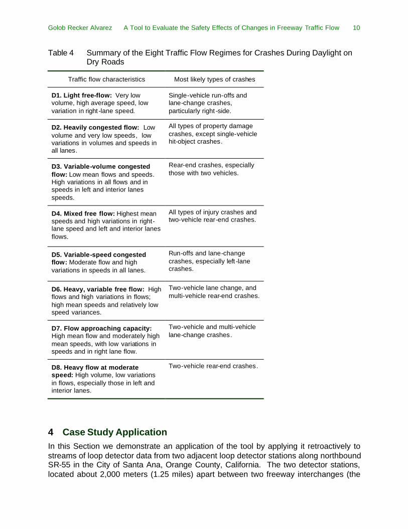
Table 4 Summary of the Eight Traffic Flow Regimes for Crashes During Daylight on Dry Roads

Traffic flow characteristics Most likely types of crashes

D1. Light free-flow: Very low volume, high average speed, low variation in right -lane speed.

Single-vehicle run-offs and lane-change crashes, particularly right -side.

D2. Heavily congested flow: Low volume and very low speeds, low variations in volumes and speeds in all lanes.

All types of property damage crashes, except single-vehicle hit-object crashes.

D3. Variable-volume congested flow: Low mean flows and speeds. High variations in all flows and in speeds in left and interior lanes speeds.

Rear-end crashes, especially those with two vehicles.

D4. Mixed free flow: Highest mean speeds and high variations in right- lane speed and left and interior lanes flows.

All types of injury crashes and two-vehicle rear-end crashes.

D5. Variable-speed congested flow: Moderate flow and high variations in speeds in all lanes.

Run-offs and lane-change crashes, especially left -lane crashes.

D6. Heavy, variable free flow: High flows and high variations in flows; high mean speeds and relatively low speed variances.

Two-vehicle lane change, and multi-vehicle rear-end crashes.

D7. Flow approaching capacity: High mean flow and moderately high mean speeds, with low variations in speeds and in right lane flow.

Two-vehicle and multi-vehicle lane-change crashes.

D8. Heavy flow at moderate speed: High volume, low variations in flows, especially those in left and interior lanes.

Two-vehicle rear-end crashes.

4 Case Study Application In this Section we demonstrate an application of the tool by applying it retroactively to streams of loop detector data from two adjacent loop detector stations along northbound SR-55 in the City of Santa Ana, Orange County, California. The two detector stations, located about 2,000 meters (1.25 miles) apart between two freeway interchanges (the


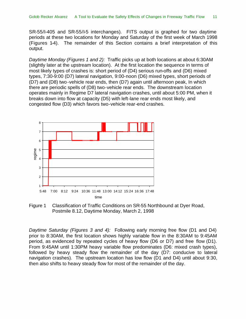
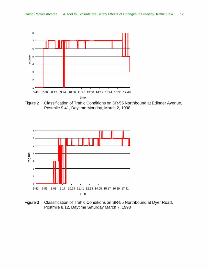
SR-55/I-405 and SR-55/I-5 interchanges). FITS output is graphed for two daytime periods at these two locations for Monday and Saturday of the first week of March 1998 (Figures 1-4). The remainder of this Section contains a brief interpretation of this output. Daytime Monday (Figures 1 and 2): Traffic picks up at both locations at about 6:30AM (slightly later at the upstream location). At the first location the sequence in terms of most likely types of crashes is: short period of (D4) serious run-offs and (D6) mixed types, 7:30-9:00 (D7) lateral navigation, 9:00-noon (D6) mixed types, short periods of (D7) and (D8) two-vehicle rear ends, then (D7) again until afternoon peak, In which there are periodic spells of (D8) two-vehicle rear ends. The downstream location operates mainly in Regime D7 lateral navigation crashes, until about 5:00 PM, when it breaks down into flow at capacity (D5) with left-lane rear ends most likely, and congested flow (D3) which favors two-vehicle rear-end crashes.

1

2

3

4

5

6

7

8

5:48 7:00 8:12 9:24 10:36 11:48 13:00 14:12 15:24 16:36 17:48

time

regi

me

Figure 1 Classification of Traffic Conditions on SR-55 Northbound at Dyer Road,

Postmile 8.12, Daytime Monday, March 2, 1998

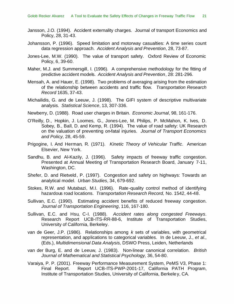
Daytime Saturday (Figures 3 and 4): Following early morning free flow (D1 and D4) prior to 8:30AM, the first location shows highly variable flow in the 8:30AM to 9:45AM period, as evidenced by repeated cycles of heavy flow (D6 or D7) and free flow (D1). From 9:45AM until 1:30PM heavy variable flow predominates (D6: mixed crash types), followed by heavy steady flow the remainder of the day (D7: conducive to lateral navigation crashes). The upstream location has low flow (D1 and D4) until about 9:30, then also shifts to heavy steady flow for most of the remainder of the day.


1

2

3

4

5

6

7

8

5:48 7:00 8:12 9:24 10:36 11:48 13:00 14:12 15:24 16:36 17:48

time

regi

me

Figure 2 Classification of Traffic Conditions on SR-55 Northbound at Edinger Avenue,

Postmile 9.41, Daytime Monday, March 2, 1998

1

2

3

4

5

6

7

8

5:41 6:53 8:05 9:17 10:29 11:41 12:53 14:05 15:17 16:29 17:41

time

regi

me

Figure 3 Classification of Traffic Conditions on SR-55 Northbound at Dyer Road,

Postmile 8.12, Daytime Saturday March 7, 1998


1

2

3

4

5

6

7

8

5:41 6:53 8:05 9:17 10:29 11:41 12:53 14:05 15:17 16:29 17:41time

regi

me

Figure 4 Classification of Traffic Conditions on SR-55 Northbound at Edinger Avenue,

Postmile 9.41, Daytime March 7, 1998

5 Demonstration of the Tool In this section, we offer a demonstration of the methodology developed in this research. Because of systematic biases introduced by non-reporting loop stations (as well as with the sample of crashes used to estimate the models), the following is intended for demonstration purposes only; no claim is made that the results are representative of actual conditions. We consider a freeway segment, S, during some time interval, T, containing n loop stations, , 1,2,il i n= K . Let itR denote the regime in the vicinity of loop station , 1,2,il i n= K , during 30-second time interval 1,2, , 30sect T= K . Ostensibly, each regime itR defines traffic flow conditions prevailing on a section of freeway extending from the midpoint between loops

1 and i il l− and loops 1 and i il l + during the 30-second time interval t. The FITS program can easily determine itR from 30-second loop count data, based on the membership functions that led to the regime classifications for dry roads during daylight or dusk-dawn, dry roads at nights, and wet roads, respectively. The total population of regimes defined by 30-second loop counts on freeway segment S during T is simply 30secTSN nT= . The number of occurrences of any particular

regime R in the population is { }| , , ;R it itn R R R i S t T R= = ∀ ∈ ∀ ∈ ∈ R , where R is the set

of regimes (which may be further broken down by particular environmental


segmentation, e.g., { }Dry Day Dry Darkness Wet− −=R R R R ). An estimate, ˆRn , of Rn can be

obtained as follows:

1. Draw a random sample of SampleN 30-second regimes. Each such sample requires 27.5 minutes of preceding loop data to calculate regime membership.

2. Compute { }| , ;Sample SampleR l ln R R R l N R= = ∀ ∈ ∈ R , We note Sample Sample

RR

n N∈

=∑R

.

3. Compute the frequency of occurrence of regime R in the sample, Sample Sample Sample

R Rf n N= .

4. Compute an estimate of Rn as ˆ Sample Sample SampleR R TS R TSn f N n N N= ⋅ = ⋅ .

An output of FITS represents the distribution of crash typologies (for crashes contained in the database on which the analysis was performed) relative to the various regimes that were identified by the analysis. Specifically, it is possible to assign each of the specific crash typologies (e.g., type, location severity) of each of the crashes contained in the database to a particular regime. So, for example, we can compute from the accident database and the analysis results:

basebase CR

CR baseC

Nf

N=

where frequency distribution of database accidents of typology relative to Regime ,

Total number of database accidents of typology assigned to Regime by FITS, and

Total number

baseCR

baseCR

baseC

f C R

N C R

N

=

=

= of database accidents of typology .C

From the TASAS database, it is possible to identify the total number of crashes of typology C that have occurred on any freeway segment S during a specified time interval T (e.g., number of fatal collisions on I-5 in Orange County during the morning peak period of the year 1998), say CTSN . Then, CTS CTS TSf N N= is the frequency distribution of crashes of typology C per 30-second loop count occurring on freeway segment S during time T. And, ˆ ˆ/ /C base base

R CR CTS R CR CTS TS Rf N n f f N nρ = ⋅ = ⋅ ⋅ is an estimate of the expected number of crashes of typology C per occurrence of regime R on freeway segment S during time T. Finally, an estimate of the expected number of crashes of typology C, ˆ C

accidentN , is given by ˆ ˆC Caccident R R

R

N nρ= ⋅∑

As a demonstration of this procedure, we consider crashes occurring during the morning peak hours on the six major freeways in Orange County, CA, using the year 1998 as a base, and compare expected crashes resulting from a hypothetical change in traffic flow conditions . There are a total of 551 loop stations on these freeways; the weekday morning peak comprises 6:00AM to 9:00AM inclusive, yielding a total of


51,573,600 TSN = regime occurrences. For purposes of this example, we make the simplifying assumption that all of these occurrences correspond to dry conditions. A total of 895SampleN = of the random sample of 30-second regimes occurred during the dry weekday morning peak hours. The expected distribution of these among the eight Dry-Day regimes is given in Table 5. Suppose that, through traffic control measures, we were able to virtually eliminate the two “congested flow” regimes (D2 and D3), transferring these previously congested periods to the “heavy, steady flow” Regime D7. The expected distribution of Dry-Day regimes under this scenario is shown in the fourth column of Table 5. Table 5 Distribution of Dry-Day Regimes in the Random Sample

R SampleRn ˆ Sample Sample

R R TSn n N N= ⋅ ˆForecastRn

D1 113 6,511,527 6,511,527

D2 35 2,016,845 0

D3 43 2,477,838 0

D4 186 10,718,089 10,718,089

D5 47 2,708,334 2,708,334

D6 198 11,409,579 11,409,579

D7 209 12,043,444 16,538,127

D8 64 3,687,945 3,687,945

SampleN 895 TSN = 51,573,600 TSN = 51,573,600

The distribution of crash types in the analysis database with respect to the eight Dry-day regimes is given in Table 6. Calculations of base

CRf may be obtained directly from this Table. There were a total of 9,341CTSN = reported crashes on the six major Orange County freeways during 1998. Of these, 1,639 occurred during the AM weekday peak hours between 6:00AM and 9:00AM. The distribution by crash type is given in Table 7.


Table 6 Distribution of Crash Type with respect to the eight Dry-Day Regimes

Dry Day Regimes Crash Type

D1 D2 D3 D4 D5 D6 D7 D8 Total %

single veh. hit object 29 15 24 46 56 72 49 22 313 38.2

2 +veh. hit object 18 9 18 28 31 50 24 8 186 22.7

2 veh. lane-change 16 17 12 32 13 21 17 18 146 17.8

3 +veh. lane-change 3 7 7 10 4 3 4 4 42 5.13

2 veh. rear-end 1 23 15 23 2 6 2 14 86 10.5

3 + veh. rear-end 1 14 5 9 2 7 3 5 46 5.62

Total 68 85 81 148 108 159 99 71 819

% 8.3 10.3 9.89 18.0 13.1 19.4 12.0 8.67 100

Table 7 CTS CTS TSf N N= for Crash Type for the eight Dry-Day Regimes

Crash Type Frequency CTS CTS TSf N N=

single veh hit object 102 1.97776E-06

2 +veh hit object 47 9.11319E-07

2 veh lane-change 310 6.01083E-06

3 +veh lane-change 90 1.74508E-06

2 veh rear-end 671 1.30105E-05

3 + veh rear-end 419 8.12431E-06

Total 1,639

From the information in these tables we can calculate the respective

ˆ/C baseR CR CTS TS Rf f N nρ = ⋅ ⋅ and from which we calculate ˆ ˆC C

accident R RR

N nρ= ⋅∑ and their

expected distribution across the various regimes. These distributions are listed in Table 8 for crash type. The row tota ls here, by definition, match the observed values; the categorizations by regime are products of FITS. However, the model may also be used in a forecasting mode to estimate expected modifications in safety outcomes accrued from changes in flow patterns, say through reducing congestion by ramp metering. Displayed in Table 9 are the expected crashes under the new traffic flow conditions in this hypothetical example (i.e., a revised Table 8) and summaries of improvements in safety that would be expected under the above scenario. When applied in a forecast


mode, FITS does not guarantee consistency between typologies for different characteristics (crash type, location, and severity). This is because the membership functions for each typology were determined independently. Resolving such inconsistency through a combined analysis (e.g., by a two-dimensional classification scheme, such as crash type and severity) could not be supported by the sample data that was available for the present study. Table 8 ˆ ˆC C

accident R RR

N nρ= ⋅∑ for Crash Type for the eight Dry-Day Regimes

Dry day Regimes Crash Type

D1 D2 D3 D4 D5 D6 D7 D8 Total

single veh hit object 9 5 8 15 18 23 16 7 102

2 +veh hit object 5 2 5 7 8 13 6 2 47

2 veh lane-change 34 36 25 68 28 45 36 38 310

3 +veh lane-change 6 15 15 21 9 6 9 9 90

2 veh rear-end 8 179 117 179 15 47 15 109 671

3 + veh rear-end 9 127 46 82 18 64 27 46 419

Total 72 365 215 373 96 198 109 211 1,639

Table 9 Forecast ˆ ˆC C

accident R RR

N nρ= ⋅∑ for Crash Type for the eight Dry-Day Regimes

Dry day Regimes Crash Type

D1 D2 D3 D4 D5 D6 D7 D8 Forecast

Total Expected Change

single veh hit object 9 0 0 15 18 23 22 7 95 -7

2+veh hit object 5 0 0 7 8 13 8 2 42 -5

2 veh lane-change 34 0 0 68 28 45 49 38 262 -48

3+veh lane-change 6 0 0 21 9 6 12 9 63 -27

2 veh rear-end 8 0 0 179 15 47 21 109 380 -290

3+ veh rear-end 9 0 0 82 18 64 37 46 256 -163

Total 72 0 0 373 96 198 150 211 1,099 -539


6 Conclusions and Directions for Further Research We have developed a tool, called FITS (Flow Impacts on Traffic Safety), that can be used to assess the changes in traffic safety tendencies that result from changes in traffic flow. The only input that FITS requires is a stream of 30-second observations from single inductive loop detectors. FITS can be used as part of any evaluation that compares before and after traffic flow data, as measured by single loop detectors. Such an evaluation might involve assessing the benefits of ATMS operations. Another application might be to compare the same section of roadway during different time periods or under different weather/lighting conditions. FITS is meant to complement existing performance measurement tools such as PeMS (Chen, et al., 2001, Choe, Skabardonis, Varaiya, 2002, Varaiya, 2001). FITS applies only to urban freeways with at least three lanes in each direction. In particular, the statistical models that underlie the tool have been estimated using historical data for freeways in Orange County, California. We presume that the relationships uncovered are indicative of all California urban freeways, particularly those in the San Francisco Bay, San Diego, and Sacramento Metropolitan Areas, but validation has not yet been conducted, so we cannot confirm the degree of spatial transferability. FITS has its limitations. First, due to the quality of the historical loop detector data that were used in calibrating the tool, we were unable to include crash rates as a function of vehicle miles of travel. The historical traffic flow data were not sufficiently representative of Orange County for an entire year, because there were systematic patterns in missing data as a function of freeway route, location along each route, day of week, and week of the year. Thus, we were unable to accurately calculate the rates, in terms of vehicle miles of travel, for crashes that happened to vehicles that were exposed to different traffic flow conditions. Consequently, FITS provides information as to which types of crashes are more likely under different types of traffic flow, but does not forecast crash rates. The enhancement of FITS to include crash rates as well as types is an important subject for future research. In spite of these limitations, we believe that we have demonstrated that FITS can be used to gain insight into how changing traffic flow conditions affect traffic safety. To the extent that changed conditions are due to ATMS operations, or other projects that influence traffic operations, FITS can be used in evaluating the effectiveness of such projects. FITS can also be used as a forecasting tool combined with simulation studies of the likely future conditions; FITS can be used to evaluate the safety conditions of alternative scenarios of operations with different ATMS or infrastructure treatments. Due to the problem with missing traffic flow data for 1998, it is strongly recommended that FITS be re-calibrated with more recent crash and traffic flow data before any large-scale deployment of this tool.


Acknowledgements This research was funded by the California Partners for Advanced Transit and Highways (PATH) and the California Department of Transportation (Caltrans). The contents of this paper reflect the views of the authors who are responsible for the facts and the accuracy of the data presented herein. The contents do not necessarily reflect the official views or policies of the University of California, California PATH, or the California Department of Transportation.


References

Aljanahi, A.A.M., Rhodes, A.H. and Metcalfe , A.V. (1999). Speed, speed limits and road traffic accidents under free flow conditions. Accident Analysis and Prevention, 31, 161-168.

Caltrans (1993). Manual of Traffic Accident Surveillance and Analysis System. California Department of Transportation, Sacramento.

Cedar, A. and Livneh, L. (1982). Relationship between road accidents and hourly traffic flow. Accident Analysis and Prevention, 14, 19-44.

Chen, C; Petty, K.F., Skabardonis, A., Varaiya, P.P. and Jia, Z. (2001). Freeway performance measurement system: mining loop detector data. Transportation Research Record 1748, 96-102.

Choe, T., Skabardonis, A. and Varaiya, P.P (2002). Freeway performance measurement system (PeMS) : an operational analysis tool. Presented at Annual Meeting of Transportation Research Board, January 13-17, Washington, DC.

De Leeuw, J. (1985). The Gifi system of nonlinear multivariate analysis. In E. Diday, et al., eds., Data Analysis and Informatics, IV: Proceedings of the Fourth International Symposium. North Holland, Amsterdam.

Dickerson, A., Peirson, J. and Vickerman, R. (2000). Road accidents and traffic flows: An econometric investigation. Economica, 67, 101-121.

Frantzeskakis, J.M. and Iordanis, D.I. (1987). Volume-to-capacity ratio and traffic Accidents on interurban four -lane highways in Greece. Transportation Research Record, No. 1112: 29-38.

Fridstrøm, L., Ifver, J., Ingebrigtsen, S., Kulmala , R. and Thomsen, L.K. (1995). Measuring the contribution of randomness, exposure, weather, and daylight to the variation in road accident counts. Accident Analysis and Prevention, 27, 1-20.

Garber, N.J. and Gadiraju, R. (1990). Factors influencing speed variance and its influence on accidents. Transportation Research Record 1213: 64-71.

Gifi, A. (1990). Nonlinear Multivariate Analysis. Wiley, Chichester.

Golob, T.F. and Recker, W.W. (2002). Relationships among urban freeway accidents, traffic flow, weather and lighting conditions. Journal of Transportation Engineering, ASCE, in press.

Gwynn, D.W. (1967). Relationship of accident rates and accident involvement with hourly volumes. Traffic Quarterly, 21, 407-418.

Hall, J.W. and Pendleton, O.J. (1989). Relationship between V/C ratios and Accident Rates. Report FHWA-HPR-NM-88-02, U.S. Department of Transportation, Washington, DC.


Jansson, J.O. (1994). Accident externality charges. Journal of transport Economics and Policy, 28, 31-43.

Johansson, P. (1996). Speed limitation and motorway casualties: A time series count data regression approach. Accident Analysis and Prevention, 28, 73-87.

Jones-Lee, M.W. (1990). The value of transport safety. Oxford Review of Economic Policy, 6, 39-60.

Maher, M.J. and Summersgill, I. (1996). A comprehensive methodology for the fitting of predictive accident models. Accident Analysis and Prevention, 28: 281-296.

Mensah, A. and Hauer, E. (1998). Two problems of averaging arising from the estimation of the relationship between accidents and traffic flow. Transportation Research Record 1635, 37-43.

Michailidis, G. and de Leeuw, J. (1998). The GIFI system of descriptive multivariate analysis. Statistical Science, 13, 307-336.

Newberry, D. (1988). Road user charges in Britain. Economic Journal, 98, 161-176.

O’Reilly, D., Hopkin, J. Loomes, G., Jones-Lee, M. Philips, P. McMahon, K. Ives, D. Sobey, B., Ball, D. and Kemp, R. (1994). The value of road safety: UK Research on the valuation of preventing on-fatal injuries. Journal of Transport Economics and Policy, 28, 45-59.

Prigogine, I. And Herman, R. (1971). Kinetic Theory of Vehicular Traffic. American Elsevier, New York.

Sandhu, B. and Al-Kazily, J. (1996). Safety impacts of freeway traffic congestion. Presented at Annual Meeting of Transportation Research Board, January 7-11, Washington, DC.

Shefer, D. and Rietveld , P. (1997). Congestion and safety on highways: Towards an analytical model. Urban Studies, 34, 679-692.

Stokes, R.W. and Mutabazi, M.I. (1996). Rate-quality control method of identifying hazardous road locations. Transportation Research Record, No. 1542, 44-48.

Sullivan, E.C. (1990). Estimating accident benefits of reduced freeway congestion. Journal of Transportation Engineering, 116, 167-180.

Sullivan, E.C. and Hsu, C-I. (1988). Accident rates along congested Freeways. Research Report UCB-ITS-RR-88-6, Institute of Transportation Studies, University of California, Berkeley.

van de Geer, J.P. (1986). Relationships among k sets of variables, with geometrical representation, and applications to categorical variables. In de Leeuw, J., et al., (Eds.), Multidimensional Data Analysis, DSWO Press, Leiden, Netherlands

van der Burg, E. and de Leeuw, J. (1983). Non-linear canonical correlation. British Journal of Mathematical and Statistical Psychology, 36, 54-80.

Varaiya, P. P. (2001). Freeway Performance Measurement System, PeMS V3, Phase 1: Final Report. Report UCB-ITS-PWP-2001-17, California PATH Program, Institute of Transportation Studies, University of California, Berkeley, CA.


ver Boon, P. (1996). A Robust Approach to Nonlinear Multivariate Analysis. DSWO Press, Leiden.

Vickrey, W. (1969). Congestion theory and transport investment. American Economic Review, 59, 251-260.

Vitaliano, D.F. and Held, J. (1991). Road accident external effects: An empirical assessment. Applied Economics, 23, 373-378.

Zhou, M. and Sisiopiku, V.P. (1997). Relationship between volume-to-capacity ratios and accident rates. Transportation Research Record, 1581: 47-52.

A Tool to Evaluate the Safety Effects of Changes in Freeway Traffic Flow

Documents

Transcript of A Tool to Evaluate the Safety Effects of Changes in Freeway Traffic Flow