Numerical Analysis of a Two-Class Freeway Traffic Model

1

Numerical Analysis of aFreeway Traffic Model

Carlo Caligaris, Simona Sacone, Silvia Siri

Dept. of Communication, Computer and System Sciences

Via Opera Pia 13, 16145 Genova

University of Genova, Italy

Summary. This paper deals with the classic second order Payne–Whitham macroscopicmodel, commonly known as PW–Model, used to forecast the traffic conditions in a freewaystretch. The results of the model may show a misbehavior similar to the instability of thenumerical solutions of partial differential equations. Since this model comes from a partialdifferential equation system as well, we use some stability rules to point out the conditionsin order to avoid these errors in simulations. We then show the effectiveness of the proposedconditions with some numerical results.

1 Introduction

The Payne–Witham model is a macroscopic second–order model used to representthe dynamic behaviour of traffic in highways or freeways. It was developed in the 70’s[1, 2] and it has been experimented in many success cases, as described in [3, 4, 5].Strong criticisms on this theory arose as well [6].

Although this model is widely used in its discrete form, it is important to point outthat it is essentially obtained by discretizing both in time and space a set of differential(continuous) equations. It is common to work directly on the discrete model, almostforgetting the differential set: this is normally accepted as long as simulation results fit

2 Carlo Caligaris, Simona Sacone, Silvia Siri

real data. The discretization is necessary in order to numerically solve the differentialequations with finite difference approximations: this must be done taking care ofthe sampling intervals used to discretize the equation variables. The choice of thesesampling intervals is fundamental for the stability of the scheme. Remember thata numerical scheme is called stable if errors from any source are not permitted togrow as the calculation proceeds. If we use “bad” discretization intervals, we willhave an unstable numerical solution, which means a completely unusable result. Theobjective of this paper concerns the definition of some conditions in order to avoidunstable simulation results. Note that the proposed considerations are referred tothe numerical stability of a simulation tool based on a PW–Model and they do notdeal with any notion of stability (Lyapunov stability, as instance) of the representedsystem.

The paper is organized as follows. In Section 2 the PW–Model is described, bothin the discrete and differential form. Then, in Section 3 we define some boundaries forthe sampling intervals in order to avoid unstable results. Some numerical examplesare provided in Section 4 and some conclusions are drawn in Section 5.

2 The PW–Model

The Payne–Whitham model is based on simple fluid dynamics laws: the flow of cars isassimilated to the flow of a liquid in a pipe. Let us start with describing the discretemodel. Space is discretized over a domain I = {i ∈ N} and time is discretized over adomain K = {k ∈ N}. T is the time interval and ∆i is the length of a space interval.Index i indicates the i− th freeway stretch and k indicates the time interval. Usuallywe refer to a freeway stretch as to the stretch included between two different toll–houses. Actually, this choice is not mandatory and a shorter space discretization stepis often used (as a consequence, some terms of the equations will be elided). However,the toll–houses should always be at the beginning and/or at the end of a stretch.

The model has three state variables:

• vi(k)[km/h]: the mean speed of vehicles in the stretch i in the [k, k + 1) timeinterval;

• ρi(k)[veh/km]: the density of vehicles in the stretch i in the [k, k+1) time interval;• qi(k)[veh/h]: the number of vehicles flowing through section i in the [k, k+1) time

interval.

The set of equations of the PW–Model is the following:

ρi(k + 1) = ρi(k) +T

∆i

{[ρi−1(k)vi−1(k)

]+

−[ρi(k)vi(k)

]+

[ri(k) − si(k)

]}; i = 1, . . . , N ; k = 0, 1, . . . , K − 1; (1)

vi(k + 1) = vi(k) +T

τ

[Vi(ρi(k)) − vi(k)

]+

T

∆i

vi(k)[vi−1(k) − vi(k)

]+

−νT

τ∆i

ρi+1(k) − ρi(k)

ρi(k) + χ; i = 1, . . . , N ; k = 0, 1, . . . , K − 1; (2)

1 Numerical Analysis of a Freeway Traffic Model 3

Vi

(ρi(k)

)= vi,max

[1 −

(ρi(k)

ρi,max

)l]m

; i = 1, . . . , N ; k = 0, 1, . . . , K − 1; (3)

qi(k) = vi(k) · ρi(k); i = 1, . . . , N ; k = 0, 1, . . . , K − 1. (4)

The parameters τ, ν, χ, vi,max, ρi,max, l, m in Equation (2) are empirically deter-mined, while Equation (3) is the steady–state speed–density characteristic. In thefollowing, we will refer to Equation (1) as to the “first updating equation” since itupdates density for each time step. Similarly, we will refer to Equation (2) as to the“second updating equation”.

We now write the differential equations from which the discrete model is obtained.Note how the discrete model depends on the choice of the scheme used in the finitedifference approximation of derivative terms. The PW–Model is usually obtained bya “forward–backward” scheme.

Table 1 Terms of the second updating equation in differential and in discrete form

Term Differential Form Discretized Form

Convection v(x, t)∂v(x, t)

∂x

T

∆i

vi(k)[vi−1(k) − vi(k)

]

RelaxationV (ρ(x, t)) − v(x, t)

τ

T

τ

[Vi(ρi(k)) − vi(k)

]

Anticipationν2

ρ(x, t)

∂ρ(x, t)

∂x

νT

τ∆i

ρi+1(k) − ρi(k)

ρi(k) + χ

Equation (1) acts as a conservation law. In physics, a conservation law states that aparticular property of an isolated system does not change as the system evolves. Here,it states that cars in the overall freeway stretch cannot appear nor disappear withouta predefined source or sink. Considering a given stretch, each car can only come fromthe previous stretch or from the on–ramp and it can only go to the following stretchor to the off–ramp. The equation can be written as:

∂ρ(x, t)

∂t+

∂q(x, t)(ρ(x, t))

∂x= r(x, t) − s(x, t) (5)

and it is apparent that Equation (1) easily comes from the coupling of Equations (5)and (4).

Also Equation (2) depends on a differential equation; but this one is drawn byobservations and it does not have a specific physical meaning. Its expression can befound, for example, in [7]:

∂v(x, t)

∂t+ v(x, t)

∂v(x, t)

∂x=

V (ρ(x, t)) − v(x, t)

τ−

ν2

ρ(x, t)

∂ρ(x, t)

∂x. (6)

Table 1 shows, for each term of Equation (6), the corresponding one in Equation(2). Equations (3) and (4) are non–differential expressions and they can be easily


written in explicit form also in continuous domains:

V(ρ(x, t)

)= vmax(x)

[1 −

(ρ(x, t)

ρmax(x)

)l]m

; (7)

q(x, t) = v(x, t) · ρ(x, t). (8)

3 The stability conditions

Considering Equation (5), it is possible to observe that it can be assimilated to theclassic first order hyperbolic partial differential equation:

∂u(x, t)

∂t+ a ·

∂u(x, t)

∂x= 0 (9)

where u(x, t) is a regular function.Let z be obtained from the discretization of u; we can use different approximation

schemes to compute the values of the equation, such as the following:

zi(k + 1) − zi(k)

T+ a

zi(k) − zi−1(k)

∆i

= 0 (10)

which can be written as:

zi(k + 1) = [1 − aλ]zi(k) + aλzi−1(k) (11)

where (as in [8]) λ is defined as:

λ ,T

∆i

. (12)

It can be proved that, in these equations, the Courant Number

µ , a · λ = a ·T

∆i

(13)

directly influences the stability of the numerical solution. A necessary condition forstability is the CFL (Courant, Friedrichs, Lewy, [9]) condition:

|µ| ≤ 1. (14)

This is the constraint that pairs of T and ∆i must always satisfy. In the followingwe will define analogous conditions for the PW–Model by working on some qualitativeconsiderations and without a rigorous mathematical approach. However, following thecommon practice for this kind of research, we will prove validity of our results byshowing their application on a simulation tool.

In this case we consider the homogeneous equation assuming that values of enteringand leaving vehicles do not influence the stability behavior. We can now rewriteEquation (5) and slightly modify it by a simple derivative property:

∂ρ(x, t)

∂t+ q′(ρ(x, t))

∂ρ(x, t)

∂x= 0. (15)


By inspecting (9) and (15) we can compare the term q′(ρ(x, t)) with the term a,which is directly involved in the Courant Number. Obviously, a is a constant, whileq′(ρ(x, t)) is a function of the density. However, if we can evaluate this function overthe interest domain, we will find the critical values which get the Courant Numbernear to 1. These values can be obtained from max {q′(ρ(x, t))}.

We use (8) and (7) to write an explicit function of q(ρ); in these calculations wewill omit the dependencies of the state variables on (x, t), simplifying the notation:

q(ρ) = ρ · v = ρ · vmax

[1 −

(ρ

ρmax

)l]m

(16)

and:

q′(ρ) = vmax

[1 −

(ρ

ρmax

)l]m

− vmaxm

[1 −

(ρ

ρmax

)l]m−1

l

(ρ

ρmax

)l

. (17)

Remembering (13) and (14) we impose

∣∣∣∣a(ρ) ·T

∆i

∣∣∣∣ ≤ 1, which means:

∣∣∣∣ max {a(ρ)} ·T

∆i

∣∣∣∣ ≤ 1. (18)

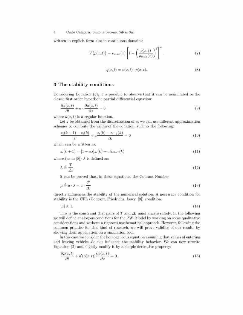
First, we study a(ρ) to find an explicit form of all the terms in (18). We can seea qualitative plot of this function in Figure 1. This plot has been drawn using somestandard values for the various parameters.

0

0

ρ[veh/km]

a(ρ)|a(ρ)|

ρρmax

vmax

Fig. 1 Plot of a(ρ)

To find the absolute maximum of a(ρ) in [0, ρmax] we must take into account the

boundary values and the absolute value coming fromda(ρ)

dρ= 0. Note how we do not

use the absolute value function in order to keep differentiability. In this way, actually,we will search for the minimum value of the function. We begin by calculating thederivative term. The solution is (ρ, a(ρ)), where:

ρ = eln s

l · ρmax, with s =

(1 + l

1 + ml

); (19)


and:

a = a(ρ)

= vmax

[(1 − s)m − (1 − s)m−1 · m · s · l

]. (20)

So, the absolute maximum value in the considered interval is:

max {a(0), |a(ρ)|, a(ρmax)} = max {vmax, |a|, 0}. (21)

Assuming that at least one parameter is greater than zero (vmax should alwaysbe, by its own definition), we can consider only the first two terms of the maximumfunction. In Figure 1, a is greater than vmax, but we want to know whether this isalways true. To find an answer, we must solve |a| > vmax, as follows:

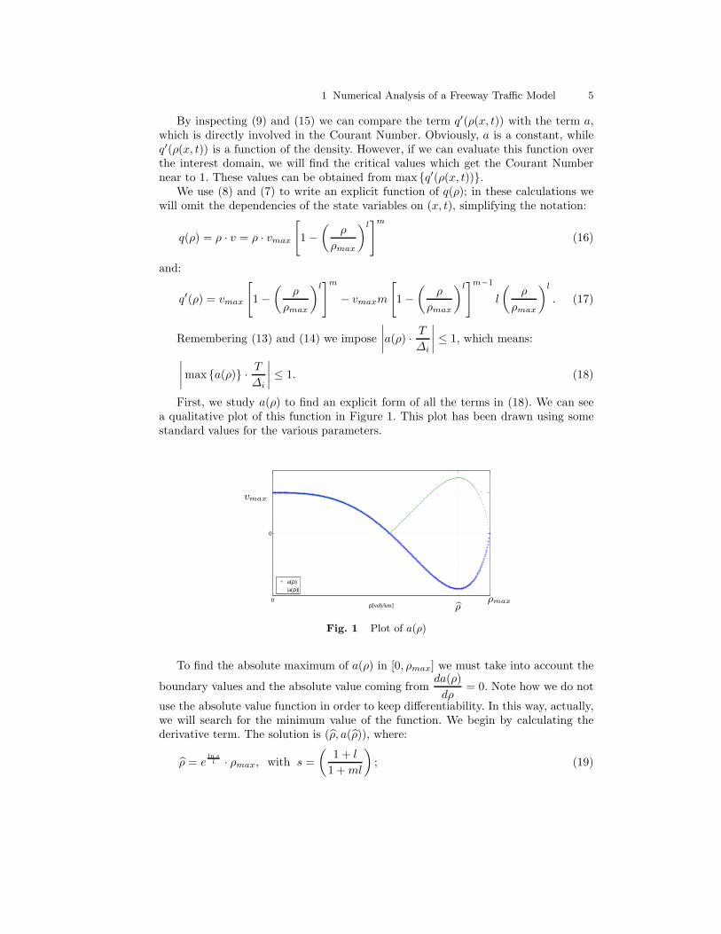
|(1 − s)m − (1 − s)m−1 · m · s · l| > 1 (22)

and its solution is:∣∣∣∣

(ml − l

ml + 1

)m−1

· (−l)

∣∣∣∣ > 1. (23)

It is not possible to explicit (23) as a function of l or m but we can plot it in aninterest domain and see when it is greater than 1. Some typical values for l and mare, respectively, 3 and 1.8. In Figure 2 we plot Equation (23) in the following domainintervals: l ∈ [0, 6] and m ∈ [0, 3.6]. Note that the plot is not always greater than 1.However, in a restricted domain, centered in the suggested values of l and m, it ispossible to state that the surface is often greater than 1.

0 0.51.8 2.5

3.6 0

23

4

6

01

l

m

Fig. 2 Plot of Equation (23)

As shown in Figure 1, the value found with the derivative term is generally higherthan the one on the left boundaries, being so the absolute maximum in the considereddomain. However, this is not always true, so we write the final condition for this firstdifferential equation in its more general form. Stability, for this only equation, isassured if:


max {vmax, |a|} ·T

∆i

≤ 1. (24)

The study for the second updating equation is very close to the one just analysed.We recall Equation (2). Again, we consider its homogeneous form, since it soundsreasonable that it does not affect the stability of the numerical solution. Actually, theanticipation term (see Table 1) contains a derivative as well. In this work we elideit together with the other non–homogenous terms since experimental results show usthat this is not a problem.

The homogeneous second updating equation looks like an inviscid Burger’s Equa-tion whose general form follows:

∂v(x, t)

∂t+ v(x, t)

∂v(x, t)

∂x= 0. (25)

If we look at this equation as to the general form of the Burger’s Equation, v(x, t)is a regular function; but we choose the name of the variable for being also our speedfunction. We can see that this is just our second updating equation. Almost everydiscretization scheme for this equation needs the following condition for stability:

∣∣∣∣T

∆i

· vmax

∣∣∣∣ ≤ 1, (26)

which is quite similar to Equation (13). Actually, it is much easier to study stabilityin this case. In fact, it can be noticed that the stability condition depends on theparameter vmax: this is a parameter of our model and it is always greater than zero.Thus, Equation (26) is the stability condition for the second updating equation.

Finally, we can couple the two constraints we have found, coming from the twohomogeneous differential equations of the model. If we look at Equations (24) and(26), we can state that the second one is included in the first. Thus, since we mustimpose the stability of the two equations, we can say that (24) assures the neededrequirements for both of them.

Then, we can state that the stability condition for the classic PW–Model is:

max {vmax, |a|} ·T

∆i

≤ 1. (27)

It is common to consider the model parameters as fixed numbers, to be foundduring the modelling phase. Furthermore, T is usually imposed by the system we aremonitoring, being the interarrival time of our data; so, it depends on the electronicsystem used on the road. ∆i is likely the only value we can change in order to make oursystem stable. If we choose a constant space discretization step, then the constraintcould be rewritten as follows:

∆i ≥ max {vmax, |a|} · T. (28)

If we want to use a variable discretization step, then we will have to face thefollowing condition:

maxi

{∆i} ≥ max {vmax, |a|} · T. (29)


4 Example

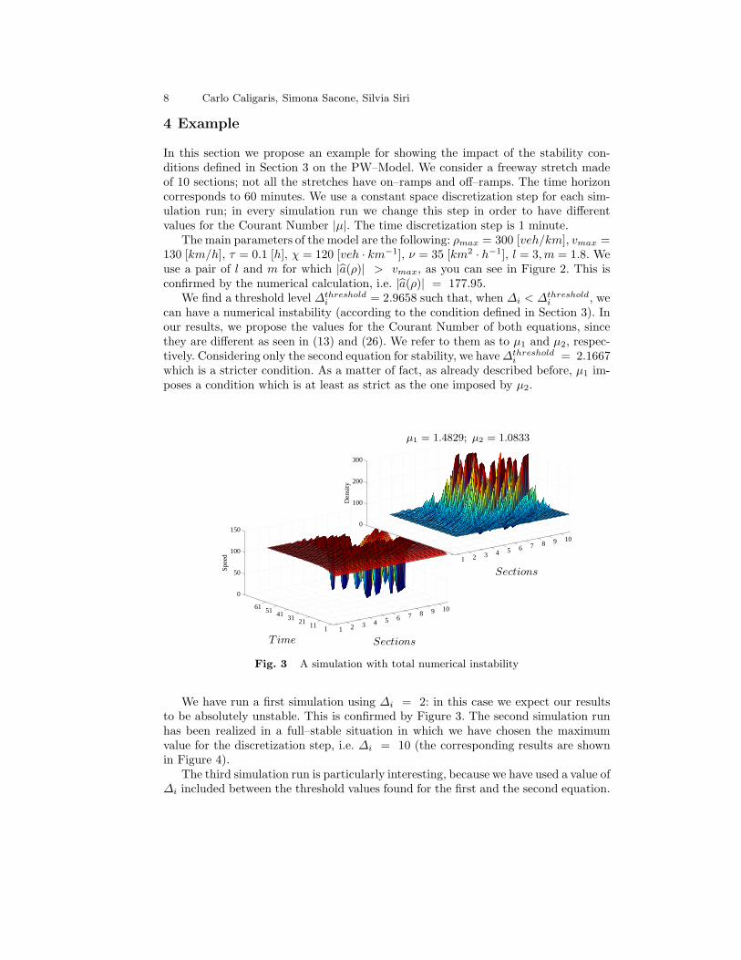
In this section we propose an example for showing the impact of the stability con-ditions defined in Section 3 on the PW–Model. We consider a freeway stretch madeof 10 sections; not all the stretches have on–ramps and off–ramps. The time horizoncorresponds to 60 minutes. We use a constant space discretization step for each sim-ulation run; in every simulation run we change this step in order to have differentvalues for the Courant Number |µ|. The time discretization step is 1 minute.

The main parameters of the model are the following: ρmax = 300 [veh/km], vmax =130 [km/h], τ = 0.1 [h], χ = 120 [veh · km−1], ν = 35 [km2 · h−1], l = 3, m = 1.8. Weuse a pair of l and m for which |a(ρ)| > vmax, as you can see in Figure 2. This isconfirmed by the numerical calculation, i.e. |a(ρ)| = 177.95.

We find a threshold level ∆thresholdi = 2.9658 such that, when ∆i < ∆threshold

i , wecan have a numerical instability (according to the condition defined in Section 3). Inour results, we propose the values for the Courant Number of both equations, sincethey are different as seen in (13) and (26). We refer to them as to µ1 and µ2, respec-tively. Considering only the second equation for stability, we have ∆threshold

i = 2.1667which is a stricter condition. As a matter of fact, as already described before, µ1 im-poses a condition which is at least as strict as the one imposed by µ2.

1 2 3 4 5 6 7 8 9 10

1112131415161

0

50

100

150

Spee

d 1 2 3 4 5 6 7 8 9 10

0

100

200

300

Den

sity

µ1 = 1.4829; µ2 = 1.0833

Sections

SectionsT ime

Fig. 3 A simulation with total numerical instability

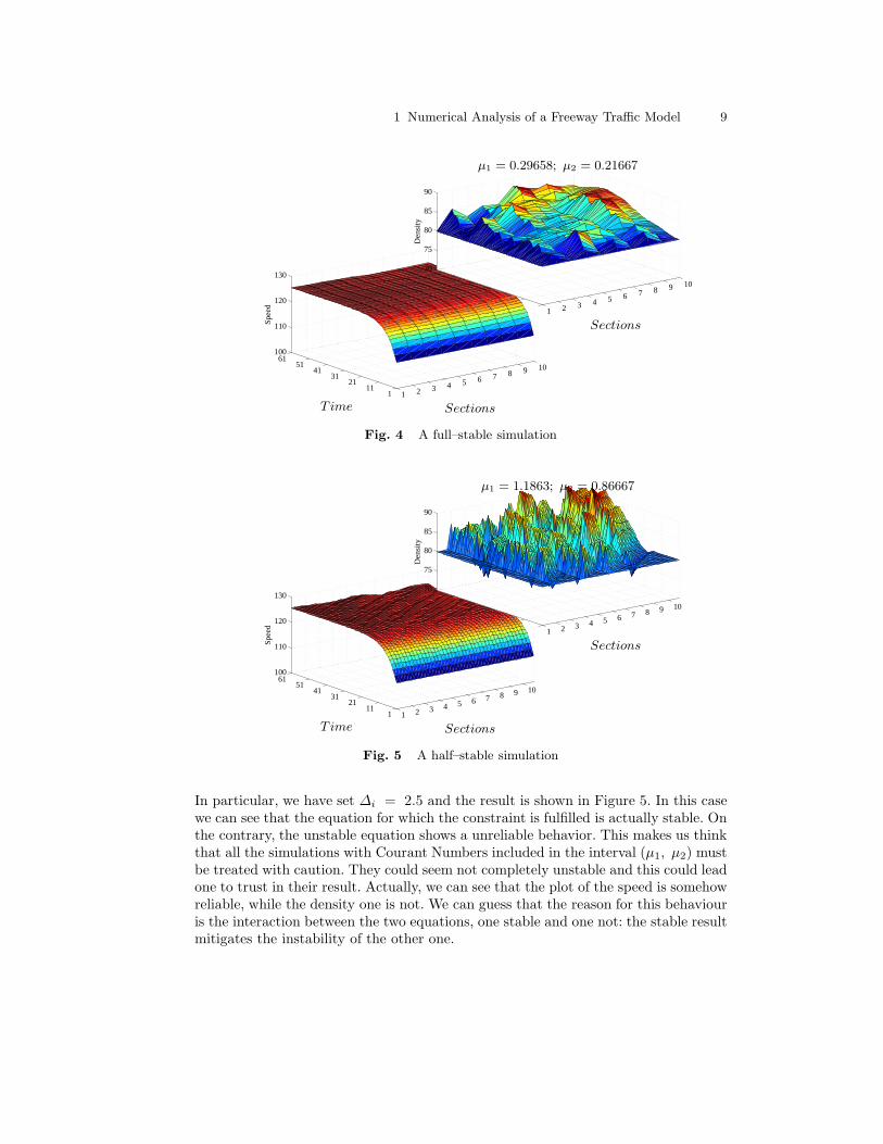
We have run a first simulation using ∆i = 2: in this case we expect our resultsto be absolutely unstable. This is confirmed by Figure 3. The second simulation runhas been realized in a full–stable situation in which we have chosen the maximumvalue for the discretization step, i.e. ∆i = 10 (the corresponding results are shownin Figure 4).

The third simulation run is particularly interesting, because we have used a value of∆i included between the threshold values found for the first and the second equation.


1 2 3 4 5 6 7 8 9 10

111

2131

4151

61100

110

120

130Sp

eed

1 2 3 4 5 6 7 8 9 10

70

75

80

85

90

Den

sity

µ1 = 0.29658; µ2 = 0.21667

Sections

SectionsT ime

Fig. 4 A full–stable simulation

1 2 3 4 5 6 7 8 9 10

111

2131

4151

61100

110

120

130

Spee

d

1 2 3 4 5 6 7 8 9 10

70

75

80

85

90

Den

sity

µ1 = 1.1863; µ2 = 0.86667

Sections

SectionsT ime

Fig. 5 A half–stable simulation

In particular, we have set ∆i = 2.5 and the result is shown in Figure 5. In this casewe can see that the equation for which the constraint is fulfilled is actually stable. Onthe contrary, the unstable equation shows a unreliable behavior. This makes us thinkthat all the simulations with Courant Numbers included in the interval (µ1, µ2) mustbe treated with caution. They could seem not completely unstable and this could leadone to trust in their result. Actually, we can see that the plot of the speed is somehowreliable, while the density one is not. We can guess that the reason for this behaviouris the interaction between the two equations, one stable and one not: the stable resultmitigates the instability of the other one.


5 Conclusions

The possibility of adopting the PW–Model for forecasting traffic behaviour on freewaystretches is subject to the definition of some suitable numerical constraints on thevalues of the discretization intervals. The fulfillment of such constraints guarantees aproper use of the model within simulation tools, that is the definition of a tool in whichno numerical instability phenomena happen. In this paper, the necessary conditionsin order to avoid numerical instability in the simulations have been derived and theireffectiveness has been shown by means of some numerical examples.

References

1. H. J. Payne, “Models of freeway traffic and control”, Mathematical Models of PublicSystems, Simulation Council Proceedings, 1971, pp. 51-61.

2. G. B. Whitham, Linear and Nonlinear Waves, John Wiley, New York, 1974.3. M. Cremer and M. Papageorgiou, “Parameter identification for a traffic flow model,”

Automatica, vol. 17, pp. 837-843, 1981.4. M. Papageorgiou, “Some remarks on macroscopic traffic flow modelling”, Transportation

Research Part A: Policy and Practice, vol. 32, pp. 323-329, 1998.5. A. Kotsialos, M. Papagergiou, C. Diakaki, Y. Pavlis and F. Middelham, “Traffic flow

modeling of large-scale motorway networks using the macroscopic modeling tool metanet”,IEEE Transactions on Intelligent Transportation Systems, vol. 3, pp. 282-292, 2002.

6. C. F. Daganzo, “Requiem for second-order fluid approximations of traffic flow”, Trans-portation Research B: Methodological, vol. 29, pp. 277-286, 1995.

7. T. Bellemans, B. De Schutter and B. De Moor, “Models for traffic control,” Journal A,vol. 43, pp. 13–22, 2002.

8. L. N. Trefethen, Finite Difference and Spectral Methods for Ordinary and Partial Differ-ential Equations, C. University, Ed., 1996.

9. H. L. R. Courant, K. Friedrichs, “On the partial difference equations of mathematicalphysics”, IBM J., vol. 11, pp. 215-234, 1967.

Numerical Analysis of a Two-Class Freeway Traffic Model

Documents

Transcript of Numerical Analysis of a Two-Class Freeway Traffic Model