Modeling present and future freeway management strategies:

variable speed limits, lane-changing and platooning of connected autonomous vehicles

Marcel Sala Sanmartí

ADVERTIMENT La consulta d’aquesta tesi queda condicionada a l’acceptació de les següents condicions d'ús: La difusió d’aquesta tesi per mitjà del r e p o s i t o r i i n s t i t u c i o n a l UPCommons (http://upcommons.upc.edu/tesis) i el repositori cooperatiu TDX ( h t t p : / / w w w . t d x . c a t / ) ha estat autoritzada pels titulars dels drets de propietat intel·lectual únicament per a usos privats emmarcats en activitats d’investigació i docència. No s’autoritza la seva reproducció amb finalitats de lucre ni la seva difusió i posada a disposició des d’un lloc aliè al servei UPCommons o TDX. No s’autoritza la presentació del seu contingut en una finestra o marc aliè a UPCommons (framing). Aquesta reserva de drets afecta tant al resum de presentació de la tesi com als seus continguts. En la utilització o cita de parts de la tesi és obligat indicar el nom de la persona autora.

ADVERTENCIA La consulta de esta tesis queda condicionada a la aceptación de las siguientes condiciones de uso: La difusión de esta tesis por medio del repositorio institucional UPCommons (http://upcommons.upc.edu/tesis) y el repositorio cooperativo TDR (http://www.tdx.cat/?locale- attribute=es) ha sido autorizada por los titulares de los derechos de propiedad intelectual únicamente para usos privados enmarcados en actividades de investigación y docencia. No se autoriza su reproducción con finalidades de lucro ni su difusión y puesta a disposición desde un sitio ajeno al servicio UPCommons No se autoriza la presentación de su contenido en una ventana o marco ajeno a UPCommons (framing). Esta reserva de derechos afecta tanto al resumen de presentación de la tesis como a sus contenidos. En la utilización o cita de partes de la tesis es obligado indicar el nombre de la persona autora.

WARNING On having consulted this thesis you’re accepting the following use conditions: Spreading this thesis by the i n s t i t u t i o n a l r e p o s i t o r y UPCommons (http://upcommons.upc.edu/tesis) and the cooperative repository TDX (http://www.tdx.cat/?locale- attribute=en) has been authorized by the titular of the intellectual property rights only for private uses placed in investigation and teaching activities. Reproduction with lucrative aims is not authorized neither its spreading nor availability from a site foreign to the UPCommons service. Introducing its content in a window or frame foreign to the UPCommons service is not authorized (framing). These rights affect to the presentation summary of the thesis as well as to its contents. In the using or citation of parts of the thesis it’s obliged to indicate the name of the author.

PhD Thesis

Modeling present and future freeway management strategies

Variable speed limits, lane-changing and platooning of connected autonomous vehicles

Author: Marcel Sala Sanmartí

PhD Supervisor:

Dr. Francesc Soriguera Martí

PhD Program in Civil Enginnering

Civil Enginnering School of Barcelona

Universitat Politècnica de Catalunya – BarcelonaTech

Barcelona, September 2019

iii

Abstract Freeway traffic management is necessary to improve capacity and reduce

congestion, especially in metropolitan freeways where the rush period lasts several hours per day. Traffic congestion implies delays and an increase in air pollutant emissions, both with harmful effects to society. Active management strategies imply regulating traffic demand and improving freeway capacity. While both aspects are necessary, the present thesis only addresses the supply side.

Part of the research in traffic flow theory is grounded on empirical data. Today, in order to extend our knowledge on traffic dynamics, detailed and high-quality data is needed. To that end, the thesis presents a pioneering data collection campaign, which was developed in the B-23 freeway accessing Barcelona. In a Variable Speed Limits (VSL) environment, different speed limits where posted, ad-hoc, in order to observe their real and detailed effects on traffic. All the installed surveillance instruments were set to capture data in the highest possible level of detail, including video recordings, from where to count lane-changing maneuvers. With this objective, a semi-automatic method to reliably count lane changes form video recordings was developed and is presented in the thesis.

Data analysis proved that the speed limit fulfillment was only relevant in sections with enforcement devices. In these sections, it is confirmed that, the lower the speed limit, the higher the occupancy to achieve a given flow. In contrast, the usually assumed mainline metering effect of low speed limits was not relevant, even for speeds as low as 40 Km/h. This might be different in case of stretch enforcement (e.g. travel time control). These findings mean that, on the one hand, VSL strategies aiming to restrict the mainline flow on a freeway by using low speed limits will need to be applied carefully, avoiding conditions as the ones presented here. On the other hand, VSL strategies trying to get the most from the increased vehicle storage capacity of freeways under low speed limits might be rather promising.

Results also show that low speed limits increase the speed differences across lanes for moderate demands. This, in turn, also increases the lane changing rates. The conclusion is that VSL strategies aiming to homogenize traffic and reduce lane changing activity might not be successful when adopting low speed limits. In contrast, lower speed limits widen the range of flows under uniform lane flow distributions, so that, even for moderate to

iv 

low demands, the under-utilization of any lane can be avoided. Further analysis of lane-changing activity allowed unveiling that high lane-changing rates prevent achieving the highest flows. This inverse relationship between the lane-changing rate and the maximum freeway throughput is modeled in the thesis using a stochastic model based on Bayesian inference. This model could be used as a control tool, in order to determine which level of lane-changing activity can be allowed to achieve a desired capacity with some level of reliability.

Previous results identify drivers' fulfillment of traffic regulations as a weak point in order to maximize the benefits of current management strategies, like VSL or lane-changing control. This is likely to change in the near future with the irruption of Autonomous Vehicles (AV) in freeways. V2X communications will allow directly actuating on individual vehicles with high accuracy. This will open the door to new management strategies based on simultaneous communication to groups of AVs and extremely short reaction times, like platooning, which stands out as a strategy with a huge potential to improve freeway traffic. Strings of AVs traveling at extremely short gaps (i.e. platoons) allow achieving higher capacities and lower energy consumption rates. In this context, the thesis presents a parsimonious macroscopic model for AVs platooning in mixed traffic (i.e. platoons of AVs travelling together with human driven vehicles). The model allows determining the average platoon length and reproducing the overall traffic dynamics leading to higher capacities. Results prove that with a 50% penetration rate of AVs in the lane, capacity could reach 3400 veh/h/lane under a cooperative platooning strategy.

Dr. Francesc Soriguera

v

Resum Per tal de millorar la capacitat i reduir la congestió a les autopistes cal

gestionar el trànsit de manera activa. Les estratègies de gestió activa del trànsit (ATMS – Active Traffic Management Strategies en les seves sigles anglosaxones) són d’especial importància en autopistes metropolitanes, on els períodes amb elevada demanda s’allarguen durant moltes hores del dia. La congestió provoca retards i un increment del consum de combustible que va lligat a unes majors emissions de gasos contaminants, tots amb efectes perniciosos per la societat. La gestió activa del transit requereix regular la demanda i millorar la capacitat de la via. Encara que tots dos aspectes son necessaris, la present tesis només analitza la gestió de l’oferta.

Part de la recerca en l’anàlisi i la teoria del trànsit es basa en dades empíriques. Actualment, per tal de millorar el nostre coneixement sobre els efectes dinàmics que es produeixen en un flux de trànsit, es requereixen bases de dades detallades i d’alta qualitat. Per satisfer aquest requeriment, aquesta tesis presenta una campanya pionera de recol·lecció de dades. Les dades es van recollir a l’autopista B-23 d’accés a Barcelona, en el marc d’experimentació amb límits de Velocitat Variable (VV). La campanya va consistir en establir diferents límits de velocitat ad-hoc, amb l’objectiu d’observar els seus efectes en el trànsit, amb tot detall. Tots els instruments de mesura es van configurar per tal de registrar les dades amb el major nivell de detall possible, incloent les càmeres de videovigilància, d’on es varen extreure els comptatges de canvi de carril. Amb aquest objectiu, es va desenvolupar una metodologia semiautomàtica per comptar canvis de carril a partir de gravacions de trànsit, que es presenta en el cos de la tesi.

L’anàlisi de les dades obtingudes ha demostrat que el compliment dels límits de velocitat només resulta rellevant en aquelles seccions que compten amb un radar. És en aquestes seccions on s’ha confirmat que com menor és el límit de velocitat, major es l’ocupació per a un flux donat. Per contra, la hipòtesi habitual de que uns límits de velocitat baixos produeixen una restricció del flux no es va observar de forma rellevant, ni tan sols amb límits tant baixos com 40 Km/h. Aquest comportament podria esser diferent en el cas d’implantar un radar de tram. Aquests resultats signifiquen que, per una banda, les estratègies de VV que es basen en una restricció del flux en una autopista mitjançant límits de velocitat baixos, cal que siguin emprades amb cautela, evitant les condicions presentades en la tesi. Per altra banda, les

vi 

estratègies de VV que exploten la capacitat d’emmagatzemar vehicles a l’autopista quan es rebaixen els límits de velocitat, resulten prometedores.

Els resultats obtinguts també mostren com les diferències de velocitats entre carrils s’incrementen per a límits de velocitat baixos i en condicions de demanda moderada. Això, alhora, incrementa el nombre de canvis de carril. La conclusió és que les estratègies d’homogeneïtzació del trànsit basades en VV poden no obtenir els resultats desitjats quan s’adopten límits de velocitat baixos. Per contra, els límits de velocitat baixos contribueixen a una distribució de flux més uniforme entre carrils, de forma que es pot evitar la infrautilització de carrils, inclús per demandes moderades o baixes. L’anàlisi més detallat de l’activitat de canvi de carril demostra que una taxa elevada de canvis de carril impedeix assolir fluxos grans de circulació. En la tesi, aquesta relació inversa entre la taxa de canvis de carril i el flux màxim de trànsit a l’autopista s’ha modelat de forma estocàstica utilitzant un model basat en la inferència Bayesiana. Aquest model es pot utilitzar com una eina de control, per tal de determinar quina taxa de canvi de carril es pot permetre si es vol assolir una capacitat determinada amb una determinada probabilitat de compliment.

En vista dels resultats previs, la falta de compliment de les normes de trànsit per part dels conductors s’identifica com un punt dèbil a l’hora de maximitzar els beneficis de les actuals estratègies de gestió del transit, com la VV o el control de canvi de carril. Això probablement canviarà en el futur pròxim amb la irrupció dels Vehicles Autònoms (VA) a les autopistes. Els sistemes de comunicació V2X permetran actuar individualment sobre cada vehicle amb una gran precisió. Això obrirà la porta a noves estratègies de gestió, basades en la comunicació simultània entre diferents grups de VA i en temps de reacció extremadament curts, com per exemple és el “platooning”, que destaca pel seu gran potencial per millorar el trànsit en autopista. Els “platoons” son cadenes de VA viatjant amb uns espaiaments extremadament curts que permeten assolir capacitats mes elevades i un menor consum energètic. En aquest context, la tesi presenta un model macroscòpic parsimoniós per a “platoons” de VA en condicions de transit mixt, és a dir, compartint la infraestructura amb vehicles tradicionals. El model permet determinar la longitud mitjana dels “platoons” i reproduir la dinàmica general del trànsit que repercuteix en majors capacitats. Per exemple, els resultats mostren que amb una penetració de VA del 50% en el carril, la capacitat pot assolir 3400veh/h/carril sota una estratègia de “platoon” cooperatiu.

Dr. Francesc Soriguera

vii

Acknowledgements  

First of all I acknowledge the funding received form the projects (TRA2013-45250-R/CARRIL) and (TRA2016-79019-R/COOP) that not only have made this thesis possible in the first place. But they also provided the resources to divulgate the results in different congresses and assist to several courses. This enabled to get some very useful feedback from researchers of other institutions, get new ideas, and learn new techniques, overall improving the quality of the research done during the thesis.

En el moment d’escriure aquestes paraules la tesis ja esta quasi enllestida. Fer una tesi doctoral es ha sigut un gran repte personal i professional. L’exigència del repte fa que en alguns moments un es qüestioni si va prendre la dedició correcta quan va decidir posar-s’hi. La resposta no es mai fàcil, però amb el temps te’n adones que les recompenses arriben, tarden mesos o anys, però acaben arribant. Així doncs a part del gran repte intel·lectual que representa aprendre nous coneixements, noves eines i diferents tècniques d’investigació. Hi ha el repte afegit, d’acceptar que la investigació, com tot el que es important a la vida no es immediat, sinó el fruit de l'esforç i la perseverança al llarg del temps.

Aquesta etapa no hagués estat possible sense el meu director de tesi, el Francesc Soriguera. Aprendre la seva forma de fer recerca m’ha ajudat a no perdre més temps del necessari en algunes tasques, encara que algun cop m’hagi calgut equivocar-me primer. També la insistència de que en la recerca cal perseverar ha ajudat a superar alguns dels moments més foscos de la tesis. I sobretot, perquè sinó hagués sigut per ell, que em va introduir en el món de la recerca en la tesina de final de carrera, de ben segur no hagués fet el doctorat, per tot, gràcies.

Gràcies també a tots els companys del despatx i els del CENIT amb qui vaig compartir experiències els primers anys. Al Cèsar i l’Hugo que quan vaig començar la tesi i anava ben perdut em van aconsellar i orientar, tant important com tenir un bon director es tenir companys amb experiència i solvència que et guiïn en alguns dels petits detalls quotidians de la tesi. A la Irene, amb qui vaig compartir uns mesos d’investigació dels qual va sorgir una amistat, que ara està entorpida pels 9500Km que hi ha entre Barcelona i Irvine. A l’Aleix, que vàrem començar la tesi quasi junts i vàrem ser companys de penes i alegries durant un bon temps. A la Mireia, el Quique,

viii 

l’Albert i el Pau, perquè veure que altres son capaços d’arribar al final de la tesi dona força per seguir endavant. I no em puc oblidar dels que ara son es companys de despatx, el Marcos, la Marga i l’Enrique, junts hem après els uns dels altres i ens hem ajudat a fer aquest camí més fàcil.

També a tots els amics que van començar el doctorat abans que jo: Oriol, Ventura, Pitus i Eloi. La vostra experiència m’ha ajudat, sobretot el compartir les penes que no tan sovint s’expliquen com la glòria que també i és. A la família i amics en general per tenir paciència i donar suport en els moments en que un està capficat i malhumorat. Gràcies a tots, però en especial a la Laura la meva parella i ara just abans d’acabar la tesi ja la meva dona, per tota la paciència que has tingut. Als pares, Miquel i Montse, per animar-me a fer el pas quan vaig començar i tenia els meus dubtes. I a tu Jordi Tur, per totes les “sessions de running” per Collserola o Montjuïc que tant aclareixen la ment. A tots amb els que hem fet muntanya o quedat per fer uns birres no us puc enumerar, la llista seria massa llarga però gràcies igualment, per arribar a bon port tan important es treballar molt com saber desconnectar quan cal, i a vegades sort n’he tingut de la vostra insistència per fer-ho.

A tots vosaltres, moltes gràcies per tot

ix

Table of contents Abstract …………………………………………………………….…………………. iii Resum …………………………………………………………………………………… v Acknowledgments ………………………………………………………………….. vii Chapter I: Thesis overview ................................................................... 1 1. Variable Speed Limits........................................................................................ 4

Effects of VSL ................................................................................................ 5 On the lack of adequate empirical VSL data ................................................ 6

2. Lane Changing ................................................................................................... 8 Obtaining lane changing empirical data ........................................................ 9 Lane changing findings ................................................................................ 10

3. Connected autonomous vehicles ...................................................................... 11 4. The present thesis ............................................................................................ 13

Objectives .................................................................................................... 13 Delimitations ............................................................................................... 14 Thesis structure ........................................................................................... 14 Contributions ............................................................................................... 17 Publications from this thesis ....................................................................... 19

5. Bibliography .................................................................................................... 23 PART I: EMPIRICAL Chapter II: Freeway Lab: Testing Dynamic Speed Limits ................. 29 1. Introduction and background .......................................................................... 32 2. Site description and typical traffic pattern ...................................................... 34 3. DSL system and surveillance equipment installed ........................................... 34 4. The experiment ................................................................................................ 39

4.1. Experiment design ................................................................................ 39 5. Experiment results ........................................................................................... 40

5.1. Drivers’ compliance with DSL .............................................................. 44 5.2. Lane changing activity .......................................................................... 46

6. Conclusions ...................................................................................................... 47 7. Acknowledgements ........................................................................................... 47 References ............................................................................................................ 48

x 

Chapter III: Automated fundamental diagram calibration with near-stationary data .................................................................................... 51 1. Introduction ..................................................................................................... 54 2. Near stationary data ........................................................................................ 56

2.1. Automatic detection of near stationary data ........................................ 58 3. Automatic Congestion detection ...................................................................... 60 4. Obtaining the Fundamental Diagram .............................................................. 62

4.1. Calibration with near stationary data .................................................. 63 5. Results with the speed variable database ........................................................ 64 6. Conclusions and future research ...................................................................... 66 7. Acknowledgments ............................................................................................ 67 References ............................................................................................................ 67 Chapter IV: Effects of Low Speed Limits on Freeway Traffic Flow ... 71 1. Introduction and background ........................................................................... 74 2. Test site description and available data .......................................................... 81 3. Data treatment methodology: per lane stationary periods .............................. 83 4. Effects of low speed limits on the flow-occupancy diagram ............................. 85

4.1. Limitations of the Previous Analysis and Conclusions ......................... 89 5. Effects of low speed limits on inter- and intra-lane behavior .......................... 90

5.1. Effects of Low Speed Limits on Inter-Lane Traffic Flow Distribution . 90 5.2. Effects of Low Speed Limits on Inter-Lane Speed Differences .............. 94 5.4. Effects of Low Speed Limits on Lane Changing .................................... 96 5.5. Effects of Low Speed Limits on Intra-Lane Speed Variability .............. 99

6. Some remarks regarding congested states ...................................................... 101 7. Conclusions and further research ................................................................... 102 8. Acknowledgements ......................................................................................... 104 References .......................................................................................................... 104 Chapter V: Measuring traffic lane-changing by converting video into space-time still image ....................................................................... 111 1. Introduction ................................................................................................... 114 2. Traffic video processing: a state of the art .................................................... 115

2.1. Fully automated techniques ................................................................ 115 2.2. Semi-automatic video processing ......................................................... 118 2.3. Visual video processing ....................................................................... 120

3. A semi-automatic video processing method for measuring lane-changing activity ............................................................................................................... 120

xi

3.1. Constructing the epoch ....................................................................... 122 3.2. Perspective and distortion .................................................................. 123 3.3. Occlusions and shadows ...................................................................... 123 3.4. Camera settings for high quality recordings ....................................... 126 3.5. Global quality index (GPI) of the recording ....................................... 127 3.6. The Graphical User Interface (GUI) ................................................... 129

4. Application to the b-23 freeway accessing Barcelona .................................... 130 4.1. Description of the different methods used .......................................... 131 4.2. Performance of the different counting methods .................................. 131 4.3. Findings from the measured lane-changing data ................................ 136

5. Conclusions .................................................................................................... 138 6. Acknowledgements ......................................................................................... 139 Appendix 1 ........................................................................................................ 140

A1.1 Effects of distortion on a flat sensor ................................................. 140 A1.2 The perspective corrected scanline .................................................... 143

Appendix 2 ........................................................................................................ 145 A2.1 Video image quality indexes .............................................................. 145 A2.2 Video framing quality indexes ........................................................... 146 A2.3 The global quality index (GQI) ........................................................ 147

Appendix 3 ........................................................................................................ 148 A3.1 Image preprocessing and candidate extraction .................................. 148 A3.2 Classification ..................................................................................... 149

References .......................................................................................................... 150 Chapter VI: Freeway lane-changing: some empirical findings .......... 155 1. Introduction ................................................................................................... 158 2. The B-23 database ......................................................................................... 160

2.2. Lane changing database ...................................................................... 161 2.3. Data available from traffic detectors .................................................. 162

3. Lane changing: some empirical findings ........................................................ 162 3.1. Lane changing peaks in congested periods .......................................... 162 3.2. Lane changing probability vs. maximum flow .................................... 167

4. Conclusions .................................................................................................... 168 5. Acknowledgments .......................................................................................... 169 References .......................................................................................................... 170

xii 

PART II: MODELING Chapter VII: Bayesian inference stochastic model for determining freeway capacity reduction as a result of lane-changing activity ..... 173 1. Introduction ................................................................................................... 176 2. The empirical database .................................................................................. 179

2.1. Configuration of the detection zones ................................................... 180 2.2. Available data and aggregation procedures ........................................ 181

3. Descriptive analysis: congestion, shockwaves and lane-changing ................... 183 3.1 Lane-changing peaks in congested periods ........................................... 184 3.2. Lane-changing peaks in traffic regime transitions ............................... 186

4. The stochastic relationship between lane-changing and freeway capacity ..... 187 4.1 The stochastic model ............................................................................ 188 4.2 Model calibration for the B-23 case study ........................................... 192 4.3 Sensitivity analysis ............................................................................... 194 4.4 Discussion of obtained results .............................................................. 196

5. Conclusions .................................................................................................... 199 6. Acknowledgements ......................................................................................... 200 References .......................................................................................................... 200 Chapter VIII: Macroscopic Modeling of Connected Autonomous Vehicles Platoons under Mixed Traffic Conditions .......................... 209 1. Introduction and background ......................................................................... 212 2. Definitions ...................................................................................................... 213 3. Platoon length estimation .............................................................................. 214

3.1. Cooperative average platoon length .................................................... 216 3.2. Opportunistic platooning .................................................................... 216 3.3. Comparing platoon schemes. ............................................................... 219

4. Mixed lane capacity ....................................................................................... 221 5. Conclusions .................................................................................................... 222 6. Acknowledgements ......................................................................................... 223 References .......................................................................................................... 223 Chapter IX: Macroscopic model for autonomous vehicle platoons: a LWR multilane extension ................................................................. 227 1. Introduction and background ......................................................................... 230 2. Model definitions ............................................................................................ 232 3. Platoon model ................................................................................................ 234

xiii

4. Mixed traffic model, LWR adaptation .......................................................... 236 4.1. Fundamental Diagram values ............................................................. 236 4.2. Mixed lane dynamics .......................................................................... 239 4.3. Sectional dynamics and Fundamental Diagram ................................. 240 4.4. Lane changing at shock waves ............................................................ 242 4.5. A particular case, Slugs and Rabbits .................................................. 243

5. Results ........................................................................................................... 245 5.1. Example 1, same free speed. ............................................................... 249 5.2. Example 2, different free speeds ......................................................... 253

6. Sensitivity analysis on capacity ..................................................................... 254 6.1. Methodology ....................................................................................... 254 6.2. Sensitivity Analysis results ................................................................. 256

7. Conclusions and further research ................................................................... 260 8. Acknowledgements ......................................................................................... 262 Annex 1: fundamental diagram ......................................................................... 262

A1.1. Demonstration of constant characteristic wave under constant time gap ............................................................................................................. 264

Annex 2: equal gap demonstration .................................................................... 266 References .......................................................................................................... 267

xv

List of Figures

Figure 1.1. Present thesis structure and organization. ...................................... 17 

Figure 2.1. Experiment site layout diagram...................................................... 35 

Figure 2.2. Typical weekday cumulative traffic demand for the morning rush. 36 

Figure 2.3. Free flow speeds and maximum speed limits on the test site. ........ 36 

Figure 2.4. Typical weekday average sectional occupancy................................ 36 

Figure 2.5. Minute average travel times on the test site. ................................. 37 

Figure 2.6. Speed contour plot. ......................................................................... 37 

Figure 2.7. Speed limit compliance. (a)Isolated detector. (b) Detector with speed enforcement device ................................................................ 45 

Figure 2.8. Oblique cumulative count (N), occupancy (T) and lane change (L) curves at Camera 2309 and detector 20ETD(S) on 12th June 2013 (Cassidy and Windover, 1995). ....................................................... 46 

Figure 3.1. Example of how time aggregated data can produce artificial results.. ........................................................................................................ 56 

Figure 3.2. Cumulative curves for flow (black) and occupancy (blue). ............ 57 

Figure 3.3. Algorithm to select the longest near stationary periods. ................ 59 

Figure 3.4. Representation on the oblique cumulative curves of the near-stationary periods. ........................................................................... 59 

Figure 3.5. Results of the proposed algorithm to detect congestion. ................ 62 

Figure 3.6. Automatically calibrated fundamental diagram. ............................ 65 

Figure 4.2. Capacity – speed limit relationship according to different models.. 79 

Figure 4.3. Test site layout.. ............................................................................. 81 

Figure 4.4. Sectional (i.e. all lanes) Flow – Occupancy diagram for different speed limits. .................................................................................... 87 

Figure 4.5. Flow distribution across lanes.. ...................................................... 92 

Figure 4.6. Relative speed difference between adjacent lanes. .......................... 95 

xvi 

Figure 4.7. Lane changing probability between adjacent lanes ......................... 97 

Figure 4.8. Lane changing probability versus relative speed difference between adjacent lanes .................................................................................. 98 

Figure 4.9. Speed variability within the lane. ................................................. 100 

Figure 4.10. Comparison between free-flowing and congested stationary states for similar occupancy levels. .......................................................... 102 

Figure 5.1. From video to epoch. Original methodology as in (Patire, 2010). 119 

Figure 5.2. New scanline definition and epoch construction. .......................... 121 

Figure 5.3. Example of the scanline pixel selection method. ........................... 122 

Figure 5.4. Occlusion of the scanline ............................................................... 124 

Figure 5.5. Example of an aborted lane-changing maneuver .......................... 125 

Figure 5.6. Framing and scanlines for 7 different camera locations ................ 128 

Figure 5.7. Graphical User Interface. .............................................................. 129 

Figure 5.8. Evolution of error in the automatic method for different training sample sizes. .................................................................................. 135 

Figure 5.9. Evolution of error with the quality of the recording. .................... 135 

Figure 5.10. Detailed video quality indicators and resulting 𝐹1 accuracy metric ...................................................................................................... 135 

Figure 5.11. Oblique cumulative count (N), occupancy (T) and lane-changing (L) curves. N ................................................................................. 137 

Figure 5.12. Location of lane changes. ............................................................ 137 

Figure 5.A1. Graphical definition of parameters. ........................................... 140 

Figure 5.A3. Distortion effects on a flat sensor. ............................................. 142 

Figure 5.A3. Maximum and average distortion values for different 𝐹𝑂𝑉s on a flat sensor. ..................................................................................... 142 

Figure 5.A4. Algorithm for the pixel selection in the perspective corrected scanline.. ........................................................................................ 145 

Figure 5.A5. Automatic epoch processing for lane change detection. ............. 149 

Figure 6.1. B-23 schematic layout and lane numbering .................................. 160 

Figure 6.2. Flow, occupancy and lane-changing oblique cumulative plot in

xvii

congested periods .......................................................................... 163 

Figure 6.3. Bottleneck at detection zone 2305. LC data was collected on detection zone 2305. ...................................................................... 164 

Figure 6.4. Lane-changing spatio-temporal distribution in detection zone 2305 ...................................................................................................... 165 

Figure 6.5. Spatial distribution of lane-changing in detection zone 2305 for all the measuring period. .................................................................... 166 

Figure 6.6. (a) Lane-changing probability versus average flow. Note. All data computed over 5 min. aggregation period; (b) Model for the maximum number of lane-changes per km between any pair of lanes as a function of the average flow per lane. .................................... 168 

Figure 7.1. B-23 test site schematic layout and lane numbering.. .................. 182 

Figure 7.2. Different detection zone layouts. .................................................. 183 

Figure 7.3. Flow, 𝑁 𝑡 , occupancy, 𝑇 𝑡 , and lane-changing, 𝐿 𝑡 , oblique cumulative plots in congested periods. (a), (b) and (c) correspond to different days and detection zones. ............................................... 185 

Figure 7.4. Effects of the bottleneck within detection zone 2305. ................... 186 

Figure 7.5. Flow, occupancy and lane-changing oblique cumulative plots during traffic regime transitions.. ............................................................. 187 

Figure 7.6. Graphical model of the relationship between the lane-changing normalized ratio, 𝑟, and the average flow per lane, 𝑞. .................. 188 

Figure 7.7. Lane-changing normalized ratio (𝑟) versus average flow per lane (𝑞). ................................................................................................ 191 

Figure 7.8. Probability density functions of the stochastic parameters 𝛼, 𝛽 and 𝑄 for the free-flowing and congested models. ................................ 193 

Figure 7.9. Sensitivity analysis of the model specification with respect to the polynomial rates 𝛾 and 𝛿 .............................................................. 195 

Figure 7.10. Maximum lane-changing per km and hour between any pair of lanes, 𝑠, as a function of the average flow per lane, 𝑞 .................. 197 

Figure 8.1. Platoon components illustration. .................................................. 213 

Figure 8.2. Average platoon lengths under different demands, AV penetration rates and platooning schemes. ....................................................... 219 

xviii 

Figure 8.3. Comparaison between cooperative and opportunistic platooning in terms of average platoon length. a) No platoon length limit. b) Maximum length of 20 vehicles platoon. ....................................... 221 

Figure 8.4. CAV penetration rate vs lane capacity for both platooning schemes (cooperative and opportunistic) and maximum platoon length of

∞ and 20 vehicles per platoon. ................................................... 222 

Figure 9.1. Platoon definitions, from (Sala and Soriguera, 2019). ................... 233 

Figure 9.2. Average platoon lengths under different demands, AV penetration rates and platooning schemes, adapted from (Sala and Soriguera, 2019). ............................................................................................. 235 

Figure 9.3. Fundamental Diagram shapes.. .................................................... 238 

Figure 9.4. Mixed lane Fundamental Diagram example. ................................ 240 

Figure 9.5. Spatial representation of capacity consumption. ........................... 242 

Figure 9.6. Lane changing at shock waves. ..................................................... 243 

Figure 9.7. Resulting Fundamental Diagrams for: a) Slugs and Rabbits, source: Daganzo 2002a. b) Simplified resoluble by hand model. ............... 244 

Figure 9.8. Mixed lane CAV penetration rate (𝛽) vs lane capacity for opportunistic and cooperative platoons with a platoon limit of 20 vehicles and no limit. ..................................................................... 247 

Figure 9.9. Variables vs density for different AV penetration rates and platoon schemes. No platoon length limit. One mixed lane, thus 𝛼 𝛽. ... 248 

Figure 9.10. Result of example 1. a) Fundamental Diagram for the different lanes and the section. b) Mixed lane CAV penetration rate (𝛽) for different mixed lane densities. c) Average platoon (𝑜) length at different mixed lane densities. ....................................................... 250 

Figure 9.11. Space-time diagram of the temporal incident in example 1. ....... 251 

Figure 9.12. Fundamental Diagram with lane blocking incident for example 1. Letters represent the traffic sates in the Figure 9.11, subindex stands: c for cooperative and o for opportunistic. The dotted lines are the shockwaves between states. ............................................... 252 

Figure 9.13. Result for example 2 with 2-pipe flow. a) Fundamental Diagram for the different lanes and the section. b) Mixed lane CAV penetration rate (𝛽) for different mixed lane densities. c) Average platoon (𝑎) length at different mixed lane densities. .................... 253 

xix

Figure 9.14. Visual representation of why LDS (Low Discrepancy Sequences) offer a better coverage of the variable range in a 2-dimensional example with 64 point. The selected low discrepancy sequence is Sobol numbers. .............................................................................. 255 

Figure 9.15. Graphical comparison between capacity sensitivity indexes for scenario 1 (a) and scenario 2 (b). .................................................. 257 

Figure 9.16. Scenario 1 detailed sensitivity analysis for capacity, a) Capacity vs CAV time gap. b) Capacity vs total penetration rate. ................. 260 

Figure 9.17. Scenario 2 detailed sensitivity analysis for capacity, a) Capacity vs CAV free speed. b) Lane CAV penetration rate vs total CAV penetration rate. ............................................................................ 260 

Figure 9.A1. Visual representation of the microscopic variables: speed, headway, spacing, gap, time gap and vehicle length. They are shown with the trajectories of two consecutive vehicles. Vehicles travel at constant speed ................................................................ 263 

Figure 9.A2. Fundamental diagram with constant free speed, time gap and gap regions 𝑣𝑓 𝑣𝑔 0. ..................................................................... 264 

 

xxi

List of Tables

Table 1.1. Comparison among different active traffic management strategies regarding their focus. ........................................................................ 1

Table 1.2. Predicted outcomes of AV introductions, some of them can be contradictory ..................................................................................... 3

Table 2.1. Research questions to be addressed, part 1. ..................................... 41

Table 2.2. Research questions to be addressed, part 2. ..................................... 42

Table 2.3. DSL and surveillance equipment configuration. ............................... 43

Table 2.4. DSL and surveillance equipment configuration. ............................... 44

Table 4.1. Literature Review: Empirical VSL Effects on a Sectional Basis ...... 76

Table 4.2. Summary of the Per-Lane Stationary Period Estimation ................ 84

Table 4.3. Flow – Occupancy Diagram Characterization (Sectional Level) ...... 88

Table 4.4. Flow – Occupancy Diagram Characterization (Per Lane) ............... 91

Table 4.5. Lane Flow Distribution for Different Speed Limits ......................... 93

Table 5.1. Quality factors addressed in the proposed global quality index (GPI) of the recording. ............................................................................ 129

Table 5.2. Lane-changing counts from different methods and their relative errors. ............................................................................................ 133

Table 5.A1. Definition of variables and parameters in the perspective correction method. ........................................................................ 141

Table 5.A2. Video quality indexes and their lower and upper bound thresholds: 𝑞𝑗 , 𝑞𝑗 . .......................................................................................... 146

Table 5.A3. Video quality indexes applied to the cameras used in the pilot test ...................................................................................................... 148

Table 7.1. Configuration of the B-23 freeway detection zones ........................ 181

Table 7.2. Calibrated parameters of the stochastic 𝑟, 𝑞 models ...................... 192

Table 8.1. Input definitions. ............................................................................ 214

Table 8.2. Variable definitions. ....................................................................... 214

xxii 

Table 9.1. Inputs definitions. ........................................................................... 233

Table 9.2. Parameters definitions. ................................................................... 234

Table 9.3. Vehicular parameter definition for example 1. ............................... 246

Table 9.4. Bottleneck capacity and delay results ............................................ 251

Table 9.5. Example 1 solution for both types of platoon. 𝑢 is epxresed in 𝐾𝑚/ℎ and 𝑞 is measured as vehicles per hour exiting platoon lanes, thus, negative means vehicles entering platoon lanes. ............................ 252

Table 9.6. Variables in the sensitivity analysis and their range except for 𝐿𝑃. ...................................................................................................... 256

Table 9.7. 𝑆 values in scenario 1 ..................................................................... 258

Table 9.8. 𝑆 values in scenario 1 ................................................................... 258

Table 9.9. 𝑆 values in scenario 2 ..................................................................... 258

Table 9.10. 𝑆 values in scenario 2 ................................................................. 259

Table 9.A1. Available space, density and flow for RV and platoon leaders at different lanes. ............................................................................... 267

Thesis overview

1

Chapter I

Thesis overview Traffic congestion is a recurrent phenomenon around the globe. In dense developed metropolitan areas, this is a daily problem which causes productivity loss. This problem is only expected to worsen (OECD International forum, 2017). However, congestion is not only the cause of delays; it is also related to capacity loss, increased air pollution and more traffic accidents.

Traffic management strategies can be used to reduce or eliminate congestion. These, typically focus on either reduce demand or increase productivity. A brief description of some of the most common strategies is provided at Table 1.1.

Table 1.1. Comparison among different active traffic management strategies regarding their focus.

Demand management Capacity improvement Ramp metering HOV and HOT lanes Tolls

Variable Speed limits Dynamic lane management Lane changing management

Ramp metering for instance is a strategy which consists on limiting the

flow of vehicles that can enter a given facility. This is widely used in North America, where freeway ramps are long enough to accommodate the long ramp queues that might be formed. Variable Speed Limits (VSL) is a strategy where the speed limits of the freeway change according to the traffic conditions in the road. These limits are posted on electronic signals located

Chapter I 

2 

at regular intervals. The objective of the algorithm behind the VSL is typically to reduce congestion, but it can also be to improve traffic safety or to improve air quality. HOV lanes (High Occupancy Vehicles) are lanes dedicated to those vehicles that have a minimum of occupants in it. The goal of this strategy is to enable those who share a car to cut some congestion in the rush hour. Thus, actually encouraging sharing vehicles. In some cases LOV (Low Occupancy Vehicles) are allowed to use HOV lanes provided that they pay a fee. This kind of lanes is named HOT lanes (High Occupancy Toll). In most cases the price of the toll changes, so to incentivize or deter LOV demand. This is to ensure high use of the HOT lanes without actually reaching congestion. Talking of tolls, general tolls or urban tolls are also a traffic management strategy to reduce, control or shift demand through the day. For this latter case the prices need to change through the day.

Another set of strategies is dynamic lane management. This means giving different uses to a given lane according to traffic conditions. The reversible lanes fall into this category. These are lanes that change their direction. This strategy fits well in stretches where demand presents strong asymmetric patterns. Other strategies on that regard are to change the functionality of one lane. This can be for instance change one regular lane to be a HOV lane during the rush hour or to use the hard shoulder as a lane in order to speed up the congestion reduction once it has set up.

Control of lane changing maneuvers is also a useful management strategy as road capacity typically increases when lane changing is prohibited. However, as this strategy is limited to on/off states, this is only suitable in some specific locations where lane changes can actually be forbidden without strong disruption. Thus, this is mostly used in expensive linear infrastructures such as bridges or tunnels which have no on- or off-ramps.

The goal of reducing congestion is not only justified to reduce travel time, vehicular emissions, etc. But also implies increasing the freeway throughput. As when congestion appears on a road infrastructure, their capacity decreases. This phenomenon is called capacity drop, and has been observed at many locations around the globe (Banks, 1991; Cassidy and Rudjanakanoknad, 2005; Cassidy and Bertini, 1999; Chung et al., 2007; Hall and Agyemang-Duah, 1991; Oh and Yeo, 2012; Patire and Cassidy, 2011; Srivastava and Geroliminis, 2013; Yuan, et al., 2015). The magnitude of the capacity drop has been estimated to range between 3% and 18% (Oh and Yeo, 2012). So, any strategy that succeeds in keeping the road infrastructure

Thesis overview

3

in free flow for longer is actually increasing their productivity by avoiding the capacity drop.

All the described strategies are solely for freeway management, which is the scope of the present thesis. However, freeways are just a part of the greater mobility system. Thus, readers have to bear in mind that actions in other parts of the system will have its impact on freeways. Just to give some examples, improvements in mass transit systems reduce the use of private cars. Also actions in urban planning can affect freeway use. It has been studied that where land has mixed uses, both the trip length and car use are found to be smaller. Urban sprawl is also positively linked to private vehicle ownership and use.

All the presented strategies are made thinking in the paradigm of vehicles driven by humans. This means that no vehicles could possibly travel empty, limited reaction time, very limited communications between cars, thus cooperation is almost impossible to achieve, etc. Some of the strategies can be enhanced by the expected irruption of Connected Autonomous Vehicles (CAV). When CAV will be introduced, changes in mobility can go much further than just improving current management strategies. New management strategies will be available and maybe new mobility patterns will be observed. The problem is that CAV do not exist at the present day, so no one does actually know how they will actually work (behave on the road) and how the society will actually react to their introduction. This means that a lot assumptions need to be made, resulting in a wide range of predictions which sometimes can result in opposite outcomes. See table 1.2 for a summary of the main effects predicted.

Table 1.2. Predicted outcomes of AV introductions, some of them can be contradictory

Traffic improvement Traffic worsening Reduction of private car ownership. Increased use of shared vehicles. Capacity increase due to cooperation Reduced energy consumption in

platoons.

Increased use of the private vehicle. Reduced use of public transportation

alternatives. Capacity reduction due AV behavior,

prioritizing passengers comfort. Among the disruptions CAV could cause in transport systems, the ones

that share most consensus and concerns are that they will increase the total veh·Km traveled by private cars, due to either the existence of empty journeys or the increase use of the car as it will be a more appealing mean of

Chapter I 

4 

transportation. A reduction of mass transit systems is also predicted by some for the very same reason. Others predict that the ownership of private vehicles will decrease as it will be more expensive to own a car than hire an autonomous taxi. There are mixed opinions among the experts on the impact of this. Most of the controversy is focused on the fact that those services could be shared, but also most convenient that other means of transportations, so the key is to predict if the induced demand will be offset by the increase of vehicle occupation or not.

Regarding road capacity, both, reductions and increments of it are predicted. As of now, the settings of driver assist systems would produce a capacity reduction (Ntousakis et al., 2015). However, some argue that by once vehicles will be fully autonomous, they will be able to be much more aggressive than they are now, increasing capacities. Another stream of though is the option of platooning, which will surely increase road capacity and reduce energy consumption, the problem in this case is estimate the amount of the capacity increase, and the sensibility to some of the CAV parameters.

As said, the scope of this thesis focused on freeway traffic management

strategies. In particular Variable Speed Limits (VSL), lane changing restrictions and CAV platoons are analyzed through empirical data and modeling approaches. In following sections a more detailed and comprehensive explanation on the capabilities, limitations and state of knowledge of these topics is presented. This chapter ends with a section which gives the reader a summary of the goals, contributions, publications and structure of the present thesis.

1. Variable Speed Limits

One of the most widespread dynamic traffic management strategies is the variable speed limits. The basics of the system are based on having multiple traffic detectors which detect the traffic status on the freeway. These feed the Traffic Management Center (TMC) with data, which is then analyzed by an algorithm. Finally the algorithm, decides the speed limits to post on the different locations with variable speed signs. Note that both the traffic data collection and the speed limit display happen at discrete locations.

Thesis overview

5

The management of the freeway is done by establishing a series of rules when given the different inputs from the freeway sections. Algorithms can be rather simple, for instance just to post slower speed limits when weather conditions are bad or traffic is heavy. Or they can be very complex and take into account the current state of the whole freeway corridor. Nonetheless, the system logic is the same. It gathers information, analyzes it and responds by posting a speed limit.

1.1 Effects of VSL

VSL is linked to several different effects on traffic flow improvements. Some of the effects have been widely proven in different works, while others remain to be proven. The goal in this thesis is to find evidences of the unproven effects in the empirical data. The focus is set on the mainline metering capabilities of VSL and reduction of lane changing activity.

The mainline metering logic is to reduce the output of a section to a given value. Being the benefit, that this value will be the capacity of an existing bottleneck located downstream. This lets the freeway free flow at the bottleneck thus avoiding the capacity drop, which only happens at the new artificial bottleneck which is controlled to output a particular number of vehicles. This can be done with traffic lights, but then strong shockwaves appear both upstream and downstream of the control. By doing this with VSL, the same effect can theoretically be achieved by without the strong shockwaves.

Another goal is traffic homogenization. This is having the same traffic flow across all lanes in the section, this means that all lanes are equally used, and traveling at the same speed. This way discretionary lane changing is eliminated. These are those lane changes performed just to improve the drivers’ utility of the freeway.

Among the well proven effects of VSL on traffic flow and its externalities are the improvement on traffic safety, major incidents are reduced by 20-30% (Sisiopiku, 2001; Lee et al., 2006; Soriguera et al., 2013), reduction of pollutants emitted and fuel consumption when limits are enforced (Stoelhorst, 2008; Baldasano et al., 2010; Cascetta et al., 2010; Soriguera et al., 2013). Regarding traffic flow, several improvements are claimed and proved by empirical experiments, for instance traffic homogenization, which results in less fluctuations in time and space of the vehicles behavior when relatively small sped limits are imposed (70-90 Km/h). But it does not result in any significant capacity improvements (Smulders, 1990; van den Hoogen

Chapter I 

6 

and Smulders, 1994; Papageorgiou et al., 2008; Knoop et al., 2010; Heydecker and Addison, 2011; Duret et al., 2012). Some VSL strategies, and in particular the SPECIALIST (Hegyi et al., 2008; Hegyi and Hoogendoorn, 2010), have succeeded to reduce the extent of traffic shockwaves, by utilizing the fact, that when a speed limit is lowered at a given section, some additional storage of vehicles happens, as the vehicles now take more time to cover the same distance. This enables to control shockwaves in traffic, as it is possible to temporally reduce the amount of vehicles reaching the back of the shockwave.

However, some of the VSL theoretical effects remain unproved. Early theoretical works on VSL predicted that as a result of the traffic homogenization a significant improvement in capacity will happen (Zackor, 1972; Zackor 1991; Cremer, 1979). However, to the present day no evidence has been found to that end. Subcritical speed limits (<70 Km/h) are thought to reduce the capacity of the section allowing to control the output of a given section. However there is no prof or quantification of the effect. This effect could be especially interesting for relatively high limits (40-60 Km/h). As these limits are feasible to post and enforce in urban freeways. Note the difference between the mainline metering strategies and the SPECIALIST strategy. The first one represents a constant and steady reduction of the output flow, while the second can only reduce the outflow for a limited time period.

In order to prove the traffic homogenization and the mainline metering effects a suitable database is required. This is fully explained in the following sub-section.

1.2 On the lack of adequate empirical VSL data

Even if VSL was first used almost fifty years ago, some unknowns remain. This is due to the fact that few empirical data is available under some particular conditions. The amount of traffic data under VSL is enormous, but most of it is just using the particular algorithm of the given VSL corridor. This means that the corridor and the algorithm that manages it can be analyzed as a whole. However, strong difficulties arise when more general and not site and algorithm specific conclusions are desired; as is the case of the VSL mainline metering capabilities. There is no doubt that a low speed limit can reduce the throughput of a freeway, as when the speed is zero, the flow is zero too. What remains to be empirically checked is how different low speed limits do change the output flow. Since this is a crucial

Thesis overview

7

piece of information to design any control scheme. The mainline metering strategy assumes that the freeway flow-density relationship (fundamental diagram) is not significantly modified, thus, a reasonable level of restriction could be achieved even with reasonably high speed limits. Still, this has yet to be proven with existing data.

The problem is that VSL rely on algorithms that only post low speed limits nearby already congested areas. As a result the effects of low speed limits are mixed with the nearby traffic breakdown (congestion). As a result low speed limits are only posted in sections with already low speed and disrupted traffic. This makes impossible to isolate the effects of low speed limits from the already onset congestion. To that end low speed limits need to be posted ad-hoc in a highly demanded freeway well before any traffic breakdown happens. By proceeding this way will be possible to actually know the effects of low speed limits in a free flowing traffic stream. Effects of VSL over lane changing have not been addressed for the very same reason, the lack of reliable lane changing data under different speed limits.

Due to this shortage in empirical data under these specific circumstances, a data collection campaign was necessary. Nonetheless, this should be done in a very particular manner in order to obtain data that could enable to answer some of the remaining questions on VSL. To that end an experiment on a VSL corridor was carefully planned. The selection of the site was the B-23 freeway entering the city of Barcelona (Spain), which not only have set up a VSL system but also plenty of traffic detectors and video surveillance cameras among other equipment. This corridor was also suitable as it experiences high demand during peak hours.

The empirical data collection design was planned using four different scenarios. The first one was getting data using the standard VSL algorithm in the corridor set by the traffic administration. The other three were to set to a constant speed limit through the corridor for the whole rush hour. This ensures having a wide range of traffic states for a given speed limit. The three speed limits chosen where: high (maximum legal speed limit for the freeway), minimum (the minimum speed limit the traffic administration allows to be posted on the VSL system) and medium which was an intermediate scenario between both.

Chapter I 

8 

2. Lane Changing

In the present thesis lane changing is understood as the maneuver a vehicle performs to change from one lane to another one in a multilane road infrastructure such as a freeway. Lane changes in such infrastructures play several roles. The most important one is to enable the drivers to go from their origin to destination. These are known as mandatory lane changes and are those unavoidable to do at some point of the infrastructure to go from the given point A to another given point B. Another type of lane changing does exist, the discretionary lane changing, and these are all the other lane changes that happen. The key difference is that these lane changes regardless if they are done or not, the driver would arrive at their desired destination. Discretionary lane changes are done, as lane changing improves the drivers’ utility of the freeway. This can be to allow overtaking a slower vehicle in front and then return to the original lane, move a less occupied lane to drive more comfortably, move to a faster lane, etc. Multiple factors affect the discretionary lane changes. Being the current traffic conditions and the drivers’ perceptions and aggressiveness the ones of greater importance.

The problem, in terms of traffic flow, that lane changing arises is that when flowing near capacity they can be harmful for flow stability and total throughput. There is a limited understanding on the mechanisms behind this. Several factors are though to play a significant role on that. Among the simplest factor is the fact that a lane changing vehicle temporally occupies two lanes. Thus, a single car is effectively occupying the space of two cars at a given time. Nonetheless, several more elaborate explanations on other mechanisms have been made. Laval and Daganzo (2006) points that the pernicious effects of lane changing are extended at the arrival lane, where the vehicle can leave a longer than usual gap in front of it, wasting highway capacity. Another study (Coifman et al., 2006) finds out that when a vehicle changes lanes reduces travel time in the leaving lane and increases it at the arriving one. However, the problems is that the induced delay is bigger that the saved time at original lane, overall resulting in an increased average travel time each time a vehicle changes lanes. It also has been found that reduced rate of lane changing are associated with increased total sectional throughputs on the freeway (Cassidy and Rudjanakanoknad, 2005; Menendez and Daganzo, 2007; Cassidy et al., 2010; Patire and Cassidy, 2011) effectively linking the increase on lane changes to reduced capacities. The negative effects do not end here, lane changing is also linked to traffic instabilities, so lane changing has been found to be able to trigger or worsen

Thesis overview

9

traffic instabilities (Mauch and Cassidy, 2002; Wang and Coifman, 2008; Ahn and Cassidy, 2007). Unstable traffic is traffic dense enough so that a perturbation (as is a lane change) can significantly slow down the flow, staring a stop & go or at least a shockwave. As a result the research community believes that the capacity drop observed when congestion arises, is at least partly due to lane changing (Coifman et al., 2006; Duret et al., 2011, Laval et al., 2007). But the mechanisms behind both lane changing and capacity drop are not fully understood and it remains to be unequivocally proven.

At this point is clear that lane changing can be harmful for achieving a high and stable flow at freeways. However, for lower flows lane changing is actually beneficial, as drivers by changing lanes can travel at their desired speed by overtaking slower drivers. Thus, lane changing needs to be restricted only when high flows are expected. And the restrictions need to be implemented carefully, as mandatory lane changes have to be accommodated. Thus, the restrictions need to be announced properly, and leaving some spaces without them to allow mandatory lane changing.

Lane change managing, is not very used, as not only is difficult to implement, but also exists some lack of knowledge, mostly due to the difficulty on obtaining suitable empirical data to study. And suitable in this contexts means that the dataset is big enough, with several different traffic states and freeways configurations and of course the data is accurate and precise. But this as it will be explained following, is not an easy task.

2.1 Obtaining lane changing empirical data

Large, accurate and variate empirical lane changing datasets are very difficult and costly to obtain. The problem is that no automatic tool can reliably count lane changes through a long freeway stretch. Some tools do exist, but they do not have enough accuracy tracking the lateral vehicle position. As to obtain this information a tracking of the vehicle needs to be done in both time and space, as lane changes take both time and space to happen. This is why the typical punctual traffic detectors, such as loop detector cannot detect lane changing. Video recordings, however, are very adequate to get detailed information on lane changing, as it covers both space and time.

The problem video recordings have is how to extract vehicles trajectories from them. Some attempts have been made, being the most notorious the NGSIM data set (Federal Highway Administration, 2006). Still, the original

Chapter I 

10 

dataset was plagued by errors due to the limitations automatic image tracking tools have (Punzo et al., 2011; Montanino and Punzo, 2013a, 2013b, 2015; Coifman and Li, 2017). Researchers have found some of the error sources, being one of the most relevant ones, the lack of information in some parts of the video. In other words, the vehicles were too small, in amount of pixels at the video, to be tracked reliably. Note that in a video, the size of an object has to be measured in pixels, and the more pixels it has, the bigger appears in the video and more information it has to be tracked properly. This is even worse when the recording is not aerial. Note that an aerial shot is meant to be exactly from above the freeway at a reasonable high altitude so there are not any noticeable perspective effects. So, when the recording has some perspective, the vehicle and also the lanes change their size (in pixels) across the framing, being at the furthest part typically too small to be tracked reliably. Another option is to frame the freeway much closer, so this problem can be avoided. However, then the problem is that the stretch the video recording covers is too short to count lane changes.

As the automatic methods have low reliability could not be used in the present case, as highly detailed and error free data was necessary. Semiautomatic methods were the selected ones to that task, as they ease the time consuming task of counting, while keeping a high reliability. The obvious manual method is just watch the video and take notes on when (time) and where (space) a lane change happens in the video recording. This is a reasonable solution to count short periods of time, but as the count becomes larger, the time cost becomes prohibitively expensive. Since in this thesis a total of 63 hours of videos need to be counted, and some of them included 4 lanes stretches a better solution was seek. This was to convert the video into a space-time image, and count form the image. The logic behind this is fully explained at Chapter V, but the key takeaway is that this image accompanied by the video allowed saving around the 70% of counting time achieving better reliability in lane change counting than actually watching the video.

2.2 Lane changing findings

Thanks to the database collected and the methodology developed to count lane changes, some highly quality data, in terms of reliability and precision was acquired. This enabled a detailed analysis at serval locations under various freeway geometries and demand patterns. So it was possible to find that lane changing activity peaks under congested regimes, and the peak is

Thesis overview

11

even more intense at transition between free flow and congestion. However, lane changes do not always peak with the same intensity, so they are considered to be stochastic. Still a consistent relation between the average per lane flow, and the maximum intensity of lane change peaking was found, leading to a stochastic model of the maximum amount of lane changing that can be made for a given lane flow. The amount of lane changing decreases as the lane flow approaches capacity. This can be used to implement control algorithms, as the closer to capacity a section is flowing, the less lane changing can happen before traffic breaks down. So most of the lane changing needs to be moved at other sections with more remaining capacity.

3. Connected autonomous vehicles

Many automobile and technological companies are developing autonomous vehicles. The challenges to develop them are enormous, as they need to read the environment in very different circumstances. There is no doubt that driving in a dense urban area is not the same as in a low density area and in turn it is different a freeway than a mountain road. The challenges do not stop here. In sunny clear skies is a difficult problem to solve, but when visibility becomes poorer, such as in fog or at night, autonomous driving is even harder to solve. Rainy and snowy conditions are amongst the most challenging. Not only is the tire adherence to road greatly reduced, but also the visibility which not only affects the computer vision (video cameras) but also sensors such as the very commonly used LIDAR. Nonetheless, there is consensus that these problems will be eventually solved, the discussion is on how long this will take, but this question is out of the scope of the present thesis.

Thus, assuming that CAV will exist, the question is what can be done using CAVs to improve freeways’ productivity. Multiple management strategies can be thought, and for instance the strategies presented before: lane changing and VSL management, could be adapted to be more effective with CAVs, as it would be possible to actuate on single vehicles, instead of vague and simple instruction given to all vehicles through information panels. Not only that, but also the fulfillment of the selected strategies can be 100%. This means that the only limitation is the capability of the strategy to improve the freeway capacity.

Still, the margin of improvement is limited. VSL has not even proved that can improve capacity, is just a very useful tool to control freeway traffic

Chapter I 

12 

and avoid shockwaves and capacity drop to some extent. Lane changing has the capability to improve freeways capacity, but as find out in the present thesis, this is limited to flows of 2400 veh/h per lane in the best case scenario. This is the case of most of the current management strategies. The reasons of this limitation are the limited human reaction time and very limited communication between vehicles, which is limited to observe the vehicle trajectory, the turn signals and the brake light. However, CAVs can overcome these limitations. One particular strategy that benefits form these improved reaction times and communications capabilities is platooning. A platoon is just a string of vehicles traveling much closer than it would be usual thanks to the their ability to i) react very fast and ii) communicate between each other, so they can anticipate to the movements of several vehicles in front of them. The CAV impacts on capacity can be huge. As a matter of fact, an early study on CACC (Cooperative Adaptive Cruise Control) (Ntousakis et al., 2015) which can be considered as a preliminary step of platooning, shows capacities exceeding 3500 veh/h/lane per lane with a 100% of vehicles traveling using the CACC. Note that typical freeway lane capacities range between 2100 and 2300 veh/h/lane. Thus, the improvement in total throughput is over 50% by solely using CACC, being this value much greater than what can be achieved by VSL or lane change managing.

In spite of its promising capacity improvement, platoon has several drawbacks yet to overcome, most of them associated with lack of knowledge of how they will work. Among many, the most critical one is to know the space between two consecutive vehicles. It can be constant or increase as speed does. Falling into one category or another will be a matter of the use and technological maturity of the CAVs. And in any of these cases the exact numerical values remain unknown, as CAVs are still in development. As a result, is very important to know how sensible different performance indicators, such as capacity, are impacted by changes on the vehicles’ behaviors. This is addressed in the present thesis.

As with CAVs, there are many unknowns regarding platoons, as they are still not implemented. It is still not known the exact type of technology the vehicles will use to communicate between them. So, as with the inter platoon vehicle distance, the range, latency or the probability of a package being lost during the communication are not known. Uncertainty remains if those values will change in different environment and weather conditions and if so by how much. When all these questions will be answered, the intra-platoon vehicle distance can be calculated much more precisely. As for now, it remains just a guess, which in the present thesis has been estimated to be

Thesis overview

13

of 0.1 seconds, but also a sensitivity analysis on how changes in this value will affect the resulting outputs such as capacity is performed.

But unknowns in platoon are almost in each aspect. For instance, there is little knowledge on how fast they will form, as there is a trade-off between formation time and comfort and energy consumption. The faster they form, the more they have to accelerate and then brake. On the other side, the more comfortable and energy saving they form, the more time they will take. It is expected that different strategies will be implemented depending on the type of route, being the formation more aggressive in urban environments, and more conservative in rural areas. The same applies for cars vs trucks, as trucks weight much more, their accelerations need to be very conservative. The formation does not only effect the formation time, but also the total platoon length. In an environment with mixed traffic (less than 100% of CAVs) the more the CAVs can coordinate, the longer the resulting platoon can be.

As the thesis author is well aware of these problems, a robust macroscopic model to get some insights of the platoon outputs is purposed. This is a model with few calibration parameters that can easily be understood as they have a clear physical meaning. Also, most of the unknowns just translate into different calibration parameters, or can be considered by changing some of the calibration. Still, the platoon formation has been found difficult to calibrate with parameters, so two different approaches are presented, one aims to represent the worst case scenario while the other represents the best case scenario.

4. The present thesis

4.1 Objectives

The objective of the thesis is to improve knowledge on different present and future freeway management strategies. This is achieved by both, analyzing data and purposing behavior models. In particular the goals of the thesis can be summarized to answer the following research questions. They are split into those that have an empirical answer, and the ones that have a modeling answer.  

Chapter I 

14 

Empirical 1. How VSL and in particular sub-critical speed limits affects the

freeway flow? 2. Is the lane changing behavior different under different speed limits? 3. How lane changing activity changes in different traffic states and

how this impacts capacity? Modeling

4. How CAVs platoons can form and how long they would be? 5. How CAVs platoons could change freeway traffic dynamics and

capacity?

4.2 Delimitations

There are many different traffic strategies, and some of them can be combined together. This thesis has only analyzed three management options, two mainly focused on human drivers: VSL and lane change control and a last one for CAVs.

All the empirical data used in the present thesis for both VSL lane changing analysis is obtained from the B-23 data collection, which is fully explained in Chapter II. This experiment was carefully designed so the research questions 1, 2 and 3 in the objectives could be answered.

The analysis on CAV platoons relies solely on modeling, as there is no real world and full scale experiments or dataset on that regards. The modeling approach is chosen to be macroscopic, because it allows reducing the complexity of the already difficult calibration of it.

4.3 Thesis structure

The present thesis is composed of nine chapters. The first one being an introduction to the topics discussed in the following eight ones (II-IX): These last chapters contain the scientific contributions of this thesis in the form a scientific papers.

Introduction

Chapter I, which is the current one, introduces the different research topics and questions to be solved, and gives an outline of the thesis.

Variable Speed Limits

Chapter II fully describes the B-23 VSL experiment. This is a comprehensive explanation of the dataset used in all the empirical

Thesis overview

15

analysis of the thesis. This is a data set composed of data from various traffic detectors, video recordings and travel time measurements on different VSL scenarios during the morning rush hour in similar demand periods. Each day represents a different scenario with a given set of speed limits to be posted.

Chapter III presents an automated method to obtain near stationary period from dataset coming from the typical datasets. This is to reduce the time needed to perform this time consuming but very useful task to calibrate fundamental diagrams.

Chapter IV explains a detailed analysis on the effects of different speed limits, with special attention to low (i.e. sub-critical) speed limits (e.g. <70km/h). A section with a speed enforcement device is selected for the analysis, ensuring a high level of fulfillment. The effects of low speed limits have been found to produce a shift towards greater occupancies in the fundamental diagram with very small flow reductions. Also lane changing activity has been found to be more intense, especially for flows far from capacity. At capacity the activity remains at similar values or even smaller than for larger speed limits.

Lane changing

Chapter V. Here the methodology developed to reliably count lane changes from video recordings is fully presented. This is based on the conversion of the video recording to space-time still images. This method has proven to be faster and more reliably than actually watching the video. A fully automated method is also purposed, but this has smaller reliability.

Chapter VI. A detailed analysis of the data obtained from the different analyzed sections is performed, where is proved that lane changing peaks downstream of a bottleneck, supporting the theory that is a key contributor in the capacity drop. It is also found that lane changing concentrates at the shockwaves upstream and downstream of a congested state.

Chapter VII. A stochastic model of the maximum amount of lane changes for a given flow and traffic state is presented. The stochastic analysis is done using Bayesian inference techniques, as the lane changing dataset is too small to reliably obtain the probabilistic distribution. The model is calibrated by considering the parameters that minimized the deviance information criterion.

Chapter I 

16 

CAV platooning

Chapter VIII. In this chapter the average expected platoon length is computed. This is done following a series of assumptions on how the platoon will be formed, resulting in two different platoon formation schemes. The traffic state (flow, speed and density) on the platooning lane is an input to the model, as well as the CAV penetration rate in it.

Chapter IX continues the work of the previous one, by adding a dynamic traffic model under mixed traffic conditions. The model considers a road with two sets of lanes. On the one hand, there are general purpose lanes, used by traditional human driven vehicles. On the other hand, there are platooning lanes, where CAV's can form platoons. In most of the analyzed cases, traditional vehicles can also travel in platooning lanes, creating mixed traffic scenarios. Promising results on capacity improvements are obtained. However, capacity shows great sensibility on CAV penetration rate and the spacing between vehicles, and while in any case the capacity improves, it remains to be seen by how much when less uncertainty in this crucial parameter can be achieved.

After this description of the contents, is clear to the reader that the

present thesis is organized on three knowledge blocks, by order in the thesis: VSL, lane changing and CAV platoons, where VSL and lane changing share the Chapter II which is the empirical data source for both. However, there is another layer, which is the chapters that are mostly empirical, Chapters II-VI and those which are focused on modeling traffic behaviors, Chapters VII-IX. All described in the present paragraph can be visualized at the following Figure 1.1.

Thesis overview

17

Figure 1.1. Present thesis structure and organization.

4.4 Contributions

The present thesis makes the following contributions:

Collection of new empirical data under VSL conditions. Data is of excellent quality and includes individual vehicles measurement and videos for detailed measurements on some given stretches.

Em

piri

cal

Mod

elin

g

VSL

Lan

e ch

angi

ng

Chapter II: VSL data collection

Chapter III: Near-stationary data and Fundamental Diagram calibration.

Chapter IV: Effects of low speed limits in freeway traffic

Chapter V: Lane-changing retrieval from video recordings

Chapter VI: Effects of lane-changing on traffic flow

Chapter VII: Lane-changing effects on freeway capacity.

CA

V

Chapter VIII: Average CAVs platoon length estimation

Chapter IX: Macroscopic modeling of mixed freeway traffic (CAVs platooning and tradicional vehicles).

Chapter I 

18 

An automatic methodology to compute near-stationary periods from traffic data sensors such as loop detectors. This enables to have the high quality filtering of near-stationary periods without the tedious and time consuming task of having to compute them manually.

It has been proven that low speed limits (40 Km/h) under punctual enforcement have almost no ability of restricting flow (mainline metering). Also is found that traffic can be free flowing and stable in high occupancies (32.0-34.7%). These limits do homogenize the traffic when demand is high as a result of the great occupancies.

Low speed limits can increase lane changing under moderate demand and have no noticeable effect in high demand.

The thesis purposes a methodology to reliably count lane changes from video surveillance cameras. This is faster and more reliable than manually counting from the video. A fully automated method is also purposed. Being the automatic one less accurate. A series of guidelines on how to record video are given in order to achieve maximum reliability and minimum counting time and errors.

Is found form the empirical data that lane changing activity peaks in congestion. This peak is even greater at the interface between free flow and congestion.

Is also found that the maximum observable lane changing ratio, as defined in Chapter VII, decreases with lane flow increments. Meaning that the lower the flow the greater the likelihood of a given car to change lanes. This property can be exploited by control algorithms.

The maximum flow for congested regimes is smaller than the one in free flow, being this in concordance with the capacity drop observed in multiple locations around the world.

A macroscopic estimation of the expected platoon length given the traffic conditions and an assumption on how the platoon forms is given. Two main options are considered which are representative of the best case (longest platoon) and worse case (shortest platoon).

A multilane macroscopic traffic model for mixed traffic is purposed. The model has few calibration parameters to ease the calibration given the uncertainty around CAVs. Even though is able to not only

Thesis overview

19

compute the capacity under some given inputs but all traffic states in free flow and congestion.

If technology enables short time gaps (<0.1s) among platoon members, under great penetration rates the capacity will be several times greater than those observed now with human drivers.

4.5 Publications from this thesis

Chapters II to IX of the thesis are contributions that have been published, are in the process to be published or aim to be submitted to a scientific journal. Some of the results have been presented in national or international conferences. This section describes the specific role of the thesis author in each contribution. Only the presentations of the results done by the thesis author are mentioned, others exist, presented by co-authors of the papers. Chapter II: Freeway Lab: Testing Dynamic Speed Limits This paper is co-authored with Francesc Soriguera. The main author of the paper was Francesc Soriguera, leading the development of the paper with the original idea and the writing. Being the contribution of the present author the data collection and processing as well as doing the figures of the paper and giving some inputs to the main author. Chapter II is published in: Soriguera, F. and Sala, M. (2014). Freeway Lab: Testing Dynamic Speed

Limits. Procedia – Social and Behavioral Sciences 160, pp. 35-44.

Chapter III: Automated fundamental diagram calibration with near-stationary data This chapter is co-authored with Francesc Soriguera. The author of this thesis has contributed as the main author, having the main responsibility on planning and developing the methodology as well as writing the paper. The co-author has supervised the work and given some important and detailed feedback. The original idea was from the co-author, but the main author reformulated it to achieve the results presented. Chapter III is neither published nor submitted to any journal yet.

Chapter I 

20 

Parts of this chapter have been presented at:

Fundamental diagram, an automatic calibration with stationary data from traffic time aggregated data. II campus científico del FIT, Madrid, May, 2017.

Fundamental diagram, an automatic calibration with stationary data from traffic time aggregated data. EURO Winter Institute, Bressanone, February, 2017.

Chapter IV: Effects of Low Speed Limits on Freeway Traffic Flow This paper is co-authored with Francesc Soriguera, Irene Martinez and Monica Menendez. The author of this thesis has contributed as a co-author in further processing the VSL database, to count lane changes and obtain and refine the near-stationary periods, this last task being shared with Irene Martinez. It also has contributed by giving his opinion and thoughts on how to overcome some difficulties and perform the research and revisions. He has also done some of the final figures for the paper. The original idea, the lead, organization and most of the writing was done by the main author Francesc Soriguera. Co-author Irene Martinez perfomed some of the near stationary analysis as well as most of the detailed inter-lane analysis. Finally, co-author Monica Menendez shared her research expertise during the paper development and carefully revised the paper. Chapter IV is published in: Soriguera, F., Martínez, I., Sala, M. and Menéndez, M. (2017). Effects of

Low Speed Limits on Freeway Traffic Flow. Transportation Research Part C: Emerging Technologies 77, pp. 257-274

Chapter V: Measuring traffic lane-changing by converting video into space-time still image This paper is co-authored with Francesc Soriguera, Kevin Hullica and Veronica Vilaplana. The author of this thesis has contributed as the main author by developing and coding all the semiautomatic methods, as well as developing the perspective correction and image quality assessment algorithms. The initial idea was obtained in cooperation with Francesc

Thesis overview

21

Soriguera, as well as the final writing. The co-authors Kevin Hullica and Veronica Vilaplana are fully responsible to develop and implement the automatic method. Chapter V is published in: Sala, M., Soriguera, F., Huillca, K. and Vilaplana, V. (2019). Measuring

traffic lane-changing by converting video into space-time still image. Computer-Aided Civil and Infrastructure Engineering, 34(6), pp. 488-505.

Parts of this chapter have been presented at:

Semi-automatic road traffic video processing, flow and lane change counting. XII Congreso de Ingenieria del Transporte, Valencia, June, 2016.

Freeway experiment: Lane Change Counting. I campus científico del FIT, Crecedilla, May, 2015.

Chapter VI: Freeway lane-changing: some empirical findings This paper is co-authored with Francesc Soriguera. The author of this thesis has contributed as the main author by having the main idea, developing it and writing an initial version of the paper. The co-author has contributed in improving the overall paper quality by carefully reviewing it. Chapter VI is published in: Sala, M. and Soriguera, F. (2018). Freeway lane-changing: some

empirical findings. Transportation Research Procedia 33, pp. 107-114.

Parts of this chapter have been presented at:

Empirical findings regarding lane changing activity on Barcelona B-23 freeway. XIII Congreso de Ingenieria del Transporte, Gijón, June, 2018.

Chapter VII: Bayesian inference stochastic model for determining freeway capacity reduction as a result of lane-changing activity

Chapter I 

22 

This paper is co-authored with Francesc Soriguera. The author of this thesis has contributed as the main author by implementing all the logic; find the best stochastic model to fit the data and writing a first version of the paper. The original idea was discussed among both authors, as well as the task of reviewing the paper once submitted. The co-author gave some feedback when the method was being developed as well as reviewing the overall quality of the paper prior to the submission. Chapter VII is submitted and under review at: (Under review) Sala, M. and Soriguera, F. Bayesian inference stochastic

model for determining freeway capacity reduction as a result of lane-changing activity. Computer-Aided Civil and Infrastructure Engineering

Parts of this chapter have been presented at:

On the stochastic relationship between lane-changing and freeway capacity. 98th TRB Annual meeting, Washington D.C., January, 2019.

Chapter VIII: Macroscopic Modeling of Connected Autonomous Vehicles Platoons under Mixed Traffic Conditions This paper is co-authored with Francesc Soriguera. The author of this thesis has contributed by taking the lead in developing the original idea, implementing the methodology and writing the final paper. The co-author has contributed by supervising and giving inputs on the methodology development. Chapter VII is submitted at: (Under review) Sala, M. and Soriguera, F. Macroscopic Modeling of

Connected Autonomous Vehicles Platoons under Mixed Traffic Conditions. Transportation Research Procedia.

Parts of this chapter have been accepted for presentation at:

Macroscopic Modeling of Connected Autonomous Vehicles Platoons under Mixed Traffic Conditions. EWGT Meeting 2019, Barcelona, September, 2019.

Thesis overview

23

Chapter IX: Macroscopic model for autonomous vehicle platoons: a LWR multilane extension This chapter is co-authored with Francesc Soriguera. The author of this thesis has contributed by taking the lead in developing the original idea, developing and implementing the presented methodologies and writing the final paper. The co-author has supervised the methodology development and given inputs to achieve better and more robust results. Chapter IX is neither published nor submitted to any journal yet. Parts of this chapter have been presented at:

Macroscopic modeling of freeways platooning under mixed traffic conditions. : III campus científico del FIT, Crecedilla, May, 2019.

Cooperative freeway driving strategies in a mixed environment – driverless and traditional vehicles. Challenges for urban mobility, Barcelona, October, 2017.

5. Bibliography

Ahn, S. and Cassidy, M. J. (2007). Freeway traffic oscillations and vehicle lane-change maneuvers. 17th International Symposium Of Transportation and Traffic Theory.

Baldasano, J.M., M. Gonçalves, A. Soret, and P. Jiménez-Guerrero. (2010). Air pollution impacts of speed limitation measures in large cities: The need for improving traffic data in a metropolitan area. Atmospheric Environment 44(25), 2997-3006.

Banks, J. H. (1991). Two-capacity phenomenon at freeway bottlenecks: A basis for ramp metering. Transportation Research Record, 1320, 83–90.

Cascetta, E., V. Punzo and R. Sorvillo. (2010). Impact on vehicle speeds and pollutant emissions of a fully automated section speed control scheme on the Naples urban motorway. Proceedings of the 89th Annual Meeting of the Transportation Research Board, Washington D.C.

Cassidy, M. J. and Bertini, R. L. (1999). Some traffic features at freeway bottlenecks. Transportation Research Part B: Methodological, 33(1), 25–42.

Chapter I 

24 

Cassidy, M. J. and Rudjanakanoknad, J. (2005). Increasing the capacity of an isolated merge by metering its on-ramp. Transportation Research Part B: Methodological, 39(10), 896–913.

Cassidy, M. J., Jang, K. and Daganzo, C. F. (2010). The smoothing effect of carpool lanes on freeway bottlenecks. Transportation Research Part A: Policy and Practice, 44(2), 65–75.

Chung, K., Rudjanakanoknad, J. and Cassidy, M. J. (2007). Relation between traffic density and capacity drop at three freeway bottlenecks. Transportation Research Part B: Methodological, 41(1), 82–95.

Cremer, M. (1979). Der verkehrsfluss auf schnellstrassen: modelle, überwachung, regelung. Springer-Verlag.

Coifman, B. and Li, L. (2017). A critical evaluation of the Next Generation Simulation (NGSIM) vehicle trajectory dataset. Transportation Research Part B 105, 362–377.

Coifman, B., Mishalani, R., Wang, C., Krishnamurthy, S. and Harris, A. D. (2006). Impact of lane-change maneuvers on congested freeway segment delays: Pilot study. Transportation Research Record, 1965, 152–159.

Duret, A., Ahn, S., and Buisson, C. (2011). Passing rates to measure relaxation and impact of lane-changing in congestion. Computer-Aided Civil and Infrastructure Engineering, 26(4), 285–297.

Duret, A., S. Ahn and C. Buisson. (2012). Lane flow distribution on a three-lane freeway: General features and the effects of traffic controls. Transportation Research Part C, 24, 157-167.

Federal Highway Administration. (2006). Next Generation Simulation (NGSIM). http://ops.fhwa.dot.gov/trafficanalysistools/ngsim.htm

Hall, F. L. and Agyemang-Duah, K. (1991). Freeway capacity drop and the definition of capacity. Transportation Research Record, 1320, 91–98.

Hegyi, A., S.P. Hoogendoorn, M. Schreuder, H. Stoelhorst and F. Viti. (2008). SPECIALIST: A dynamic speed limit control algorithm based on shock wave theory. Proceedings of the 11th International IEEE Conference on Intelligent Transportation Systems, 827-832.

Hegyi, A., and S. P. Hoogendoorn. (2010). Dynamic speed limit control to resolve shock waves on freeways - Field test results of the SPECIALIST algorithm. Proceedings of the 13th International IEEE Conference on Intelligent Transportation Systems, 519-524.

Thesis overview

25

Heydecker, B. G. and J. D. Addison. (2011). Analysis and modelling of traffic flow under variable speed limits. Transportation Research Part C, 19(2), 206-217.

Knoop, V.L., A. Duret, C. Buisson and B. van Arem. (2010). Lane distribution of traffic near merging zones influence of variable speed limits. Proceedings of the 13th International IEEE Conference on Intelligent Transportation Systems, Madeira Island, Portugal, September 19–22, 485–490.

Laval, J. A. and Daganzo, C. F. (2006). Lane-changing in traffic streams. Transportation Research Part B: Methodological, 40(3), 251

Laval, J., Cassidy, M.J., and Daganzo, C.F. (2007). Impacts of lane changes at merge bottlenecks: a theory and strategies to maximize capacity. In: Traffic and Granular Flow’05, Springer, Berlin, Heidelberg, 577-589.

Lee, C., B. Hellinga, F. and Saccomanno. (2006). Evaluation of variable speed limits to improve traffic safety. Transportation Research Part C: Emerging Technologies 14(3), 213-228.

Mauch, M. and Cassidy, M. J. (2002). Freeway traffic oscillations: observations and predictions. Transportation and Traffic Theory in the 21st Century: Proceedings of the 15th International Symposium on Transportation and Traffic Theory, Adelaide, Australia, 16-18 July 2002, 653-673.

Menendez, M. and Daganzo, C. F. (2007). Effects of HOV lanes on freeway bottlenecks. Transportation Research Part B: Methodological, 41(8), 809–822.

Montanino, M., Punzo, V. (2015). Trajectory data reconstruction and simulation-based validation against macroscopic traffic patterns. Transportation Research Part B, 80, 82-106.

Montanino, M., and Punzo, V. (2013a). Making NGSIM data usable for studies on traffic flow theory : a multistep method for vehicle trajectory reconstruction. Transportation Research Record, 2390, 99-111.

Montanino, M., and Punzo, V. (2013b). Reconstructed NGSIM data. Retrieved from www.multitude-project.eu/exchange/101.html

Ntousakisa, I. A., Nikolosa, I. K., and Papageorgiou, M. (2014). On Microscopic Modelling of Adaptive Cruise Control Systems. 4th International Symposium of Transport Simulation-ISTS’14, 1-4 June 2014, Corsica, France.

Chapter I 

26 

OECD International transport forum (2017). ITF Transport Outlook 2017. Technical report.

Oh, S. and Yeo, H. (2012). Estimation of capacity drop in highway merging sections. Transportation Research Record, 2286(1), 111–121.

Papageorgiou, M., E. Kosmatopoulos and I. Papamichail. (2008). Effects of variable speed limits on motorway traffic flow. Transportation Research Record: Journal of the Transportation Research Board 2047, 37-48.

Patire, A. D. and Cassidy, M. J. (2011). Lane changing patterns of bane and benefit: Observations of an uphill expressway. Transportation Research Part B: Methodological, 45(4), 656–666.

Punzo, V., Borzacchiello, M., and Ciuffo, B. (2011). On the assessment of vehicle trajectory data accuracy and application to the Next Generation SIMulation (NGSIM) program data. Transportation Research Part C, 19(6), 1243–1262.

Qu, X., and Wang, S. (2015). Long-distance-commuter (LDC) lane: a new concept for freeway traffic management. Computer-Aided Civil and Infrastructure Engineering, 30(10), 815–823.

Smulders, S. (1990). Control of freeway traffic flow by variable speed signs. Transportation Research Part B 24(2), 111–132.

Sisiopiku, V. P. (2001). Variable Speed Control: Technologies and Practice. Proc., 11th Annual Meeting of ITS America, Miami.

Soriguera, F., J.M. Torné and D. Rosas. (2013). Assessment of dynamic speed limit management on metropolitan freeways. Journal of Intelligent

Transportation Systems: Technology, Planning, and Operations 17 (1), 78-90.

Srivastava, A. and Geroliminis, N. (2013). Empirical observations of capacity drop in freeway merges with ramp control and integration in a first-order model. Transportation Research Part C: Emerging Technologies, 30, 161–177.

Stoelhorst, H. (2008). Reduced speed limits for local air quality and traffic efficiency. Procedings of the 7th European Congress and Exhibition on Intelligent Transport Systems and Services. Genova.

van den Hoogen, E. and S. Smulders. (1994). Control by variable speed signs: Results of the Dutch experiment. Seventh International Conference on Road Traffic Monitoring and Control, 145-149.

Thesis overview

27

Yuan, K., Knoop, V. L. and Hoogendoorn, S. P. (2015). Capacity drop relationship between speed in congestion and the queue discharge rate. Transportation Research Record, 2491, 72–80.

Wang, C. and Coifman, B. (2008). The effect of lane-change maneuvers on a simplified car-following theory. IEEE Transactions on Intelligent Transportation Systems, 9(3), 523–535.

Zackor, H. (1972). Beurteilung verkehrsabhängiger geschwindigkeitsbeschränkungen auf autobahnen. Strassenbau und strassenverkehrstech 128, 1-61.

Zackor, H. (1991). Speed limitation on freeways: Traffic-responsive strategies. In Concise Encyclopedia of Traffic and Transportation Systems (M.Papageorgiou, ed.), Pergamon Press, Oxford, UK, 507–511.

 

   

 

Chapter II

Freeway Lab: Testing Dynamic Speed Limits

Published in Procedia – Social and Behavioral Sciences 160, 2014, pp. 35-44.

 

31

Freeway Lab: Testing Dynamic Speed Limits

Francesc Soriguera*a and Marcel Salaa

aBarcelona Innovative Transport – UPC – Barcelona Tech, Jordi Girona 1-3,

Building B1, Office 114, 08034 Barcelona, Spain. Abstract This paper presents the Dynamic Speed Limit (DSL) experiment that took place in June 2013 on the last 13 km stretch of the B-23 freeway accessing the city of Barcelona (Spain). The DSL system installed on that freeway in addition to the high density of surveillance equipment available makes this stretch a suitable highway lab. The objective of the experiment was to construct a comprehensive database of traffic engineering variables on a freeway site when different speed limits apply. Special attention was paid to ensure similar demand conditions between different scenarios. The experiment included the modification of the speed limits on a freeway segment making use of dynamic signals. Detailed measurements of vehicle counts, speeds, occupancies, lane changing maneuvers and travel times were taken. These simultaneous measurements obtained from very different types of monitoring equipment have been grouped into a single database. These include measurements from inductive loop detectors, radar, ultrasound and passive infrared non-intrusive traffic detectors, TV cameras and license plate recognition devices. The potential of this multi-source database is huge. For instance, a preliminary analysis empirically proves that drivers’ compliance with dynamic speed limits is very limited, unless speed enforcement devices are present. In addition, it is also proved that lane changing rates increase together with the occupancy level of the freeway. This comprehensive DSL database, unique in its nature, is made publicly available to the whole research community (http://bit.ly/1Q75vFB), (Soriguera and Sala, 2013) in order to use up all its information. The present paper aims to present in detail this DSL experiment and its preliminary results and to contribute in the dissemination of the resulting database. This will facilitate its analysis to any interested researcher, and would lead to a better understanding of the causes and effects of DSL strategies on freeways. Keywords: Dynamic speed limits; lane changing; freeway traffic; highway lab; empiric traffic database; Barcelona.

* Corresponding author

Chapter II

32 

1. Introduction and background

Freeway traffic control by means of dynamic speed limits (DSL) was first introduced in the early 1970s in Germany (Zackor, 1972) and one decade after in the Netherlands (Remeijn, 1982). Nowadays, DSL is a popular advanced traffic management strategy, with many test implementations in European and American metropolitan freeways (Summer and Andrew, 1990; Zarean et al., 2000; Lennie et al., 2009).

Despite a late dawn, today, the city of Barcelona (Spain) is among the pioneers in large scale implementations of DSL systems, with more than 100 km of controlled freeways. It all started in July 2007, when a 73-measure plan to improve the air quality in the metropolitan region of Barcelona was passed. The plan included the immediate reduction of the speed limits on major freeways accessing the city to 80 km/h (from the preexistent limits of 120 km/h). This was planned as the first step towards implementing a DSL system. The objective was to adapt the speed limits to the prevailing traffic and pollution conditions, maintaining the maximum of 80 km/h limit. The DSL system became operational in a test corridor in January 2009. Later, in January 2011, the maximum speed limit was increased to 100 km/h due to popular demand and keeping the election promise of the new incoming Government in Catalonia. Since then, the system has expanded to more corridors and it is expected to be completed by 2015.

In spite of its expansion and international popularity, the effects of DSL strategies are still not well-known. The usual claimed benefits imply reductions in pollutant emissions (Stoelhorst, 2008; Baldasano et al., 2010; Soriguera et al., 2013) and accident rates (Lee et al., 2006; Sultan et al., 2008), as well as congestion relief (Cremer, 1979; Smulders, 1990; Zackor and Papageorgiou, 1991). It is believed that these benefits are the result of the homogenization of traffic flow, which allows for increased capacity and/or for the avoidance of the capacity drop. However, these assertions are based on very scarce (or even inexistent) real empirical data. Works analyzing real traffic data under DSL strategies exist (Soriguera et al, 2013; Van Den Hoogen and Smulders, 1994; Papageorgiou et al., 2008; Hegyi and Hoogendoorn, 2010). In these, serious work was done with what was available. However, all of them faced difficulties in obtaining a suitable database. Data is generally obtained on a test corridor under a specific DSL control strategy, where different speed limits are displayed for different

Freeway Lab: Testing Dynamic Speed Limits

33

traffic conditions. This implies that data collected during a specific speed limit may not cover the whole range of possible traffic states. Results obtained are valid in order to test the aggregated corridor performance of a specific DSL algorithm, but conclusions on the detailed drivers’ behavior when facing different speed limits on the same infrastructure cannot be addressed in detail for all traffic conditions.

In order to understand the fundamental effects of speed limits in a freeway traffic stream, detailed data is needed. Individual vehicle data, without any type of aggregation, makes it possible to compute the homogeneity of speed and occupancy values within the traffic stream and also to count the number of lane changes. In addition, measurements must be obtained within a similar demand context and under clear and different speed limit configurations. This is the most difficult part of the problem. Probably, the only way to measure these data is running a specific experiment in a real freeway with the possibility of radically changing the speed limits from one day to the other, and setting the different scenarios specifically needed for the analysis. There are few freeways around the world capable of dynamically change speed limits and intensively equipped with the surveillance technology required to measure these detailed data. And what is worst, there are even less traffic administrations concerned enough with the scientific community research needs in order to allow such experiments on their heavily demanded freeways.

All the previous has been achieved on the B-23 freeway, accessing the city of Barcelona from the west. This corridor is heavily demanded, with daily recurrent congestion during the morning rush. On the last 13 km accessing the city, a DSL system is installed, with variable speed signs every 0.5 to 1km. The freeway surveillance equipment includes traffic detectors every 0.5 km (on average), TV cameras every 1km and license plate recognition (LPR) devices at both ends of the stretch. And what is more important, the Servei Català del Trànsit (SCT – the Catalan traffic administration) facilitated the experiment. All this makes the B-23 freeway an ideal highway lab.

The objective of the present paper is to present in detail such DSL experiment and provide access to the resultant database [http://bit.ly/1Q75vFB], (Soriguera and Sala, 2013). This will allow all the scientific community to make use of a comprehensive and unique freeway traffic database under different speed limit scenarios. The smart analysis of such data should lead to a fundamental advance in the knowledge of DSL effects and their causes.

Chapter II

34 

The rest of the paper is organized as follows. In Section 2 the layout of the freeway stretch where the experiment took place is presented. This includes the geographical location, the physical description and also the traffic demand pattern on a typical weekday morning rush. Next, in Section 3 the DSL system is presented, together with the description of all the technological equipment installed on the experiment site. Section 4 is devoted to the DSL experiment design, including its objectives, requirements and limitations. Section 5 presents a summary of the results. Finally, in Section 6 some conclusions are outlined.

2. Site description and typical traffic pattern

The DSL experiment took place during the first three weeks of June 2013 on the last 13 km stretch of the B-23 freeway in the inbound direction towards Barcelona (see Figure 2.1). This is one of the main freeways accessing the city, with recurrent daily congestion during the morning rush (from 7:00 to 10:00am). For a typical weekday, peak travel times may exceed more than 3 times the free flow travel time, of approx. 7 minutes (Travel Time Index > 3; see Figure 2.5). The total aggregated demand for the 7 to 10am period is almost 170 000 veh·km for the whole experiment stretch. Figure 2.2 shows the cumulative traffic demand during a typical weekday morning rush for each section. The importance of the freeway junction at kp 6.89 connecting the B-23 freeway with the Barcelona seaside beltway is evident. Three main bottlenecks exist on this freeway stretch. This can be seen in Figure 2.4 realizing the three zones with huge average occupancy. The first bottleneck (at kp 7.18) is caused by the merging/diverging conflicts at the major freeway junction. The second one (at kp 3.57) is a diverging bottleneck caused by an off-ramp queue spillback at this location. The third bottleneck is caused by the end of the freeway at a traffic light when entering the city of Barcelona. Figure 2.6 shows a contour plot of speeds where the congested time – space zones are clearly identified.

3. DSL system and surveillance equipment installed

Surveillance equipment properly working during the experiment period is shown in the layout diagram in Figure 2.1. All the equipment can be remotely controlled from the traffic management center (TMC). This

Freeway Lab: Testing Dynamic Speed Limits

35

includes traffic detectors every 0.5 km, capable of measuring flows, occupancies and speeds.

Figure 2.1: Experiment site layout diagram

Chapter II

36 

Figure 2.2: Typical weekday cumulative traffic demand for the morning rush.

Figure 2.3: Free flow speeds and maximum speed limits on the test site.

Figure 2.4: Typical weekday average sectional occupancy.

Freeway Lab: Testing Dynamic Speed Limits

37

Figure 2.5: Minute average travel times on the test site.

Figure 2.6: Speed contour plot. Between 7 and 10am on Tuesday. June 4th, 2013.

Several detector technologies are installed: traditional inductive double or single loop detectors (called ETD and ETD(S) detectors in the present paper) and non-intrusive detectors (called DT detectors) that obtain their measurements from 3 redundant technologies: Doppler radar, ultrasound and passive infrared detection. By default, all types of detectors compute, per lane and every minute, the total vehicle count [vehicles], the time-mean speed [km/h] (i.e. arithmetic average of individual speeds measured during the minute) and the detector occupancy [%].

Chapter II

38 

All the detectors are installed on the main trunk lanes. Only off-ramp “S7” and on-ramp “E8” are monitored. In general, there is only one ramp in between consecutive detectors so that the ramp flow could be approximately computed assuming vehicle conservation and neglecting detector drift. The settings of any type of detector can be modified in order to measure individual vehicle actuations (in addition to the default minute averages).

The detector system is complemented with TV cameras approximately every km. TMC operators use the cameras to obtain direct visual information in order to support their decisions when some incident takes place. The use of the cameras is completely visual, without any type of automatic processing of the images.

Finally, the surveillance system also includes two license plate recognition devices (LPR), at both ends of the experiment site. LPR are only installed in the middle and fast lanes. These are used to measure the travel time on the stretch. The system tries to pair the licenses read at both locations in order to compute the travel times. Results are reported as minute averages. There are some minutes without any pairing, and travel time is void. Incorrect matching or vehicles that detour or stop in between LPR devices implies the existence of outliers in these data (see Figure 2.5).

All these surveillance equipment support the DSL system. When the DSL system is active, “adequate” speed limits are computed every 5 minutes, and are posted on the dynamic signs installed on overhead gantries (called PVV in the present paper). There is a maximum speed sign for every lane, so that different speed limits could be posted for different lanes. However, by default, the DSL algorithm computes sectional (i.e. for all lanes) speed limits. The heuristics behind the DSL algorithm are simple. First, the corridor is divided into sections. Each section is defined by the dynamic speed limit sign at its upstream end, with an approximate length of 1 km. The posted speed limit for the section is then computed as the minimum amongst two values:

The average speed measured by the detectors within the section, rounded down to the closest 10 km/h multiple.

The speed limit posted in the next downstream signal increased at a rate of 10 km/h for every km of separation.

Finally, the posted speed limit cannot be lower than 40 km/h or higher than the maximum speed limit for that section. Speed limits are enforced at two spots of the corridor using radar units (see Figure 2.1).

Freeway Lab: Testing Dynamic Speed Limits

39

4. The experiment

The experiment was designed to provide the most suitable data in order to answer the research questions that remain unsolved. Tables 2.1-2.2 summarize the research questions to be addressed and the related requirements on the experiment design.

There are also some limitations that affected the design of the experiment. The first and more obvious is that, being an empirical traffic experiment, the same demand in all DSL contexts cannot be assured. The experiment design pays attention to ensure similar demands, but in real experiments this is always an issue. This problem is made worst by the fact that merging and diverging bottlenecks are predominant on the test site and its capacity depends on the merging/diverging demands. Other limitations are imposed by the technical capabilities of the TMC regarding the “special” settings of equipment. For instance, only 3 TV cameras can record simultaneously and only 4 detectors can simultaneously measure individual actuations. This imposes tight restrictions to the experiment design. Finally SCT, the traffic administration, imposed some additional limitations to the experiment in order not penalize the drivers in excess. This includes a minimum of 50 km/h speed limit in free flowing sections, and a maximum length of 5 km where this minimum speed limit could be posted simultaneously.

4.1. Experiment design

The experiment took place between 7 and 10am capturing the whole morning rush. Only Tuesdays, Wednesdays and Thursdays were candidate days for the experiment. This ensures, to some extent, a similar traffic demand on the corridor. The experiment did not take place in case of any type of previous incident upstream or downstream of the experiment site. Rain or bad weather also implied to abort the experiment.

Table 2.3 summarizes the DSL contexts and the surveillance equipment subject to special settings. Speed limit enforcement radars were active, but tickets were waived during the experiment periods. No specific information about the experiment was given to the drivers. The experiment design meets all the aforementioned restrictions.

The limited number of simultaneous equipment to measure detailed data and the length of freeway with minimum speed limits suggested dividing the test site in two parts: the outer part (comprising 32

Chapter II

40 

PVV to 22 PVV) and the inner part (13 PVV to 4 PVV). In between there is a transition zone. For each part the following scenarios are defined:

Maximum speed limit. 100 km/h for the outer part (Day#2) and 80 km/h for the inner part (Day#5).

Minimum speed limit. 50 km/h for the outer part, mostly free flowing (Day#4) and 40 km/h for the inner part, mostly congested (Day#7).

Medium speed limit. An intermediate scenario between a) and b). This is 80 km/h for the outer part (Day#3) and 60 km/h for the inner part (Day#6).

Dynamic speed limits. Servei Català del Trànsit (SCT) algorithm for the whole test site (Day#1).

All traffic detectors were set to store minute aggregations of vehicle counts, occupancy and average speed. In addition, 4 of them were configured to also measure individual actuations 3 TV cameras were selected (see Table 2.4) to record simultaneously high quality videos of their influence zones (i.e. 30 fps and 536 x 400 pixels) with the objective of counting lane changing activity. These selections were made taking into account that the resulting detailed measurements should capture different traffic conditions (i.e. congested and free-flowing), some of them should be near the enforcement devices so that the compliance with the speed limits is higher, and others should be farther apart in order to provide data to assess the effects of the enforcement. Finally, when possible they should be far apart from junctions, to avoid mandatory lane changes. LPR where set to measure per minute avg. travel times.

5. Experiment results

The experiment took place during the period comprised between May 30th and June 19th, 2013. The overall traffic demand on the corridor during the seven experiment days did not deviate more than 0.9% from the average.

Freeway Lab: Testing Dynamic Speed Limits

41

Tab

le 2

.1. R

esea

rch

ques

tion

s to

be

addr

esse

d, p

art

1.

Exp

erim

ent

requ

irem

ents

Is

des

irab

le t

o lo

ok fo

r hi

gh c

ompl

ianc

e ra

tes.

Oth

erw

ise,

the

onl

y co

nclu

sion

wou

ld b

e th

e la

ck o

f com

plia

nce.

The

refo

re s

peed

lim

it

enfo

rced

sec

tion

s ar

e pr

efer

able

for

deta

iled

anal

ysis

.

M

easu

rem

ents

nee

d to

be

take

n up

stre

am o

f so

me

bott

lene

ck (

i.e. q

ueue

d tr

affic

) an

d do

wns

trea

m o

f it

(i.e

. fre

e flo

win

g at

cap

acity)

.

It

wou

ld b

e de

sira

ble

to c

aptu

re t

he

cong

estion

ons

et a

nd d

isso

lve

peri

ods

(i.e

. the

w

hole

peak

peri

od)

C

reat

e co

ntex

ts w

here

the

spe

ed li

mit

be

com

es a

n ac

tive

bot

tlen

eck

(i.e

. im

pose

ver

y st

rict

spe

ed li

mit

s on

sec

tion

s flo

win

g ne

ar

capa

city

).

Sp

eed

limit

s on

the

exp

erim

ent

site

sho

uld

follo

w a

pre

dete

rmin

ed p

lan

whe

re m

ost

of t

he

occu

panc

y vs

spe

ed li

mit

sce

nari

os a

re

repl

icat

ed.

Des

crip

tion

D

o th

e dr

iver

s co

mpl

y w

ith

DSL

? (i

n pa

rtic

ular

w

hen

spee

d lim

its

are

low

and

tra

ffic

dens

ity

is

mod

erat

e).

W

hat

is t

he e

ffect

of e

nfor

cem

ent

devi

ces

on

driv

ers’

com

plia

nce?

C

an s

peed

lim

its

have

a p

ositiv

e ef

fect

on

bott

lene

ck c

apac

ity?

Whe

n?

C

an s

peed

lim

its

atte

nuat

e th

e ca

paci

ty d

rop

phen

omen

on in

the

tra

nsitio

n to

con

gest

ed fl

ow?

(i.e

. st

abili

ze t

he m

axim

um fl

ow).

C

an lo

w s

peed

lim

its

crea

te a

n “a

rtifi

cial

” bo

ttle

neck

?(so

tha

t th

e m

ainl

ine

flow

cou

ld b

e m

eter

ed b

y us

ing

spee

d lim

its) 

H

ow d

oes

the

flow

-den

sity

rel

atio

nshi

p ev

olve

un

der

diffe

rent

spe

ed li

mits?

H

ow t

his

affe

cts

the

queu

e ev

olut

ion?

(sh

ock

wav

esp

eeds

)

Issu

e

Dri

vers

com

plia

nce

Bot

tlen

eck

capa

city

Mai

nlin

e m

eter

ing

Fun

dam

enta

l di

agra

m

and

queu

e pr

opag

atio

n

 

Macro Effects

Chapter II

42 

Tab

le 2

.2. R

esea

rch

ques

tion

s to

be

addr

esse

d, p

art

2.

Exp

erim

ent

requ

irem

ents

In

divi

dual

veh

icle

dat

a is

nee

ded.

A

void

sec

tion

s ne

ar o

n/of

f ram

ps, w

here

la

ne o

ccup

ancy

is a

ffect

ed b

y th

e m

ergi

ng/d

iver

ging

.

A

void

sec

tion

s w

here

man

dato

ry la

ne

chan

ges

are

pred

omin

ant, n

ear

on/o

ff ra

mps

.

T

he q

ualit

y of

the

vid

eo r

ecor

ding

s sh

ould

be

eno

ugh

to c

ount

the

num

ber

of la

ne

Des

crip

tion

Is

the

veh

icul

ar s

peed

dis

trib

utio

n m

odifi

ed b

y di

ffere

nt s

peed

lim

its?

(in

tra

lane

and

acr

oss

lane

s)

Is

the

spe

ed v

aria

nce

redu

ced?

(sp

eed

hom

ogen

izat

ion)

C

an s

peed

lim

its

atte

nuat

e th

e st

op &

go

phen

omen

on?

In

cas

e it

exi

sts, d

oes

this

att

enua

tion

incr

ease

th

dih

t?

C

an s

peed

lim

its

hom

ogen

ize

the

occu

panc

ies

of

the

vari

ous

lane

s?

C

an s

peed

lim

its

redu

ce t

he d

iscr

etio

nal l

ane

chan

ging

rat

es?

Issu

e

Veh

icul

ar s

peed

di

stri

buti

on

Stop

& g

o at

tenu

atio

n

Inte

r la

ne

occu

panc

y

Lane

cha

ngin

g ra

tes

 

Micro Causes

Freeway Lab: Testing Dynamic Speed Limits

43

Table 2.3. DSL and surveillance equipment configuration.

Dynamic Speed Limit Gantry 

Day#1 Day#2 Day#3 Day#4 Day#5 Day#6 Day#7

33-66 PVV (13.15)

Transitional speed limits 32-67 PVV (12.62)

32 PVV (11.64) SCT 100 80 50 100 80 80

30 PVV (11.20) SCT 100 80 50 100 80 80

30 PVV L (11.20)

SCT 80 80 50 80 80 80

29 PVV L (10.67)

SCT 100 80 50 100 80 80

27 PVV (10.11) SCT 100 80 50 100 80 80

24 PVV (9.02) SCT 100 80 50 100 80 80

22 PVV (8.05) SCT 100 80 50 100 80 80

22 PVV L (8.05) SCT 100 80 50 100 80 80

20 PVV (7.28) SCT 80 80 50 80 80 80

20 PVV L (7.28) SCT 80 80 50 80 80 80

18 PVV (6.44) SCT 80 80 80 80 80 80

17 PVV (6.14) SCT 80 80 80 80 80 60

17 PVV L01 (5.80)

SCT 80 80 80 80 80 60

17 PVV L02 (5.34)

SCT 80 80 80 80 80 60

13 PVV (4.73) SCT 80 80 80 80 60 40

11 PVV (3.79) SCT 80 80 80 80 60 40

08 PVV (2.55) SCT 80 80 80 80 60 40

06 PVV (1.78) SCT 80 80 80 80 60 40

04 PVV (1.10) SCT 80 80 80 80 60 40

03 PVV (0.74) SCT 60 60 60 60 60 40

02 PVV (0.37) SCT 50 50 50 50 50 40

Chapter II

44 

Table 2.4. DSL and surveillance equipment configuration.

Day#1 Day#2 Day#3 Day#4 Day#5 Day#6 Day#7

TV Cameras

(High quality: 30 fps and 536x400 pixels)

2306 2312 2312 2312 2306 2306 2306

2305 2310 2310 2310 2305 2305 2305

2304 2309 2309 2309 2304 2304 2304

Raw Detectors (Individual actuations)

(ETD – Double loop detector)

(DT – Non Intrusive detector)

13(DT) 30

(ETD) 30

(ETD) 30

(ETD) 13

(DT) 13

(DT) 13

(DT)

12 (ETD)

27 (ETD)

27 (ETD)

27 (ETD)

12 (ETD)

12 (ETD)

12 (ETD)

11 (DT)

21 (ETD)

21 (ETD)

21 (ETD)

11 (DT)

11 (DT)

11 (DT)

8 (DT) 19

(ETD) 19

(ETD) 19

(ETD) 8 (DT) 8 (DT) 8 (DT)

5.1. Drivers’ compliance with DSL

Figure 2.3 shows that maximum speed limits are approximately fulfilled in average. However, if only considering the fastest lane, the speeding is notorious. Furthermore, results obtained from the experiment show that generalized speeding happens when lower than maximum speed limits are in force. In such situations, speed limits are only strictly fulfilled in the sections with radar enforcement. This is evident from Figure 2.7, where a contour plot shows the difference between the speed limit and the average speed for a given occupancy range on all the detectors in the test site. Red regions indicate speeding is the majority for that specific speed limit – occupancy cell, green indicates compliance and yellow indicates speed limit far above the average speed (i.e. ineffective speed limit). On each cell of the contour plot the percentage of the majority and the total number of observations (i.e. minutes) in the cell are shown. Results are shown for isolated detectors (far from any speed signal and enforcement device; see Figure 2.7a) and for detectors with speed enforcement (see Figure 2.7b).

Freeway Lab: Testing Dynamic Speed Limits

45

Figure 2.7: Speed limit compliance. (a)Isolated detector. (b) Detector with speed enforcement device

|𝑣 𝑣| 10 𝐾𝑚/ℎ 𝑣 𝑣 10 𝐾𝑚/ℎ 𝑣 𝑣 10 𝐾𝑚/ℎ

Chapter II

46 

The contour plot for isolated detectors (Figure 2.7a) shows a green region on the diagonal of the speed – occupancy contour plot, yellow above it and red below it. This means that average speed follows the typical speed – occupancy relationship, without caring about the speed limit in force. If speed limit happens to coincide with the average speed dictated by the prevailing occupancy level, then it is fulfilled. Otherwise, it is not. If speed limit is lower, speeding is generalized. If it is higher, it is ineffective. In conclusion, DSL do not have a generalized effect on drivers’ behavior.

On the contrary, if only sections with speed enforcement are considered (see Figure 2.7b), speeding is almost eliminated. In such situations, dynamic speed limits affect drivers’ behavior. However, the DSL system is not capable of enabling higher average speeds for high occupancy values that would lead to capacity increase. That is why the yellow region remains.

5.2. Lane changing activity

 

Figure 2.8: Oblique cumulative count (N), occupancy (T) and lane change (L) curves at Camera 2309 and detector 20ETD(S) on 12th June 2013 (Cassidy and Windover, 1995). A rough analysis of the lane changing activity indicates that the great

majority of discretionary lane changes take place during congested periods. A conclusive prove of this fact is obtained by plotting time series of the cumulative lane changing activity together with cumulative vehicle count and occupancy. Figure 2.8 shows that congestion reached Camera 2309 location around 8:30am. This can be seen by realizing the opposite trends in cumulative occupancy (slope increase in the T-curve) versus cumulative

Freeway Lab: Testing Dynamic Speed Limits

47

count (slope decrease in the N-curve) (Cassidy and Mauch, 2001). It is also clear from Figure 2.8 that the lane changing rate (slope of L-curve) increased notably once the congestion appeared. Although further research is needed, this result exemplifies the potential of the database in empirically proving ideas that until now were only assumptions.

6. Conclusions

This paper presents a comprehensive database of traffic variables on a unique freeway site when different speed limits apply and under similar traffic demand contexts. This includes simultaneous measurements from very different surveillance technologies. The resulting database is made available to the whole research community [http://bit.ly/1Q75vFB], (Soriguera and Sala, 2013) in order to provide a solid empirical ground from where to build and validate theories and models.

The availability of such an empirical database should lead to more conclusive proves in relation to the effects of DSL strategies. Possible research topics may include (but are not limited to) the DSL ability to increase bottleneck capacities and reduce the capacity drop phenomenon, or to avoid temporary restrictions within queues due to stop & go traffic and therefore increase queue discharge rates. The ability of DSL strategies to restrict the mainline flow on a freeway (i.e. mainline metering) by creating artificial bottlenecks in otherwise free flowing sections could also be investigated. Or the drivers’ compliance to dynamic speed limits, specifically when they are more counterintuitive (e.g. very low speed limits in uncongested traffic). Preliminary results show that DSL are only strictly fulfilled on section with active enforcement. Also the causes of these effects should be subject of research, like the speed harmonization under DSL, the reduction in the lane utilization variability, the reduction of discretionary lane change maneuvers, the DLS effects on traffic instabilities (i.e. stop&go) and the modification of vehicle headway or spacing distributions. Initial investigation shows that the lane changing is related to the occupancy level of the lanes.

7. Acknowledgements

The author acknowledges the collaboration of Jordi Janot and Dr. Mónica Menéndez from ETH Zurich for their work on the preliminary data

Chapter II

48 

analysis. Advice provided by Josep Maria Torné (BarcelonaTech) in the construction of the database and by Anthony Patire and Robert Campbell (PATH-UC Berkeley) and Bernat Goñi (TU Delft) in the video image processing is also acknowledged. This experiment would not have been possible without the collaboration and implication of the whole staff of the Servei Català del Trànsit. From his director Joan Josep Isern and his executive staff. to those who helped in the experiment design and execution Inma Selva. Jan Peña and specially Òscar Llatge who pushed for the experiment to become a reality. Finally. the hard work at the TMC during the experiment days of Javi Romero and Carles Argüelles (ute acc. sur acisa-aluvisa) and their staff is gratefully acknowledged. The experiment has been partially funded by the Servei Català del Trànsit (CM-12/2013) and by the Spanish Ministry of Science and Innovation (TRA2013-45250-R/CARRIL).

References

Baldasano, J.M., Gonçalves, M., Soret, A., and Jiménez-Guerrero, P. (2010). Air pollution impacts of speed limitation measures in large cities: The need for improving traffic data in a metropolitan area. Atmospheric Environment 44(25). 2997-3006.

Cassidy, M.J. and Mauch, M. (2001). An observed traffic pattern in long freeway queues. Transportation Research Part A 35(2). 143-156.

Cassidy, M.J. and Windover, J. (1995). Methodology for assessing dynamics of freeway traffic flow. Transportation Research Record 1484. 73-79.

Cremer, M. (1979). Der verkehrsfluss auf schnellstrassen: modelle. Überwachung. regelung. Springer-Verlag.

Hegyi, A. and Hoogendoorn, S.P. (2010). Dynamic speed limit control to resolve shock waves on freeways - Field test results of the SPECIALIST algorithm. Proceedings of the 13th International IEEE Conference on Intelligent Transportation Systems. 519-524.

Lee, C., Hellinga, B. and Saccomanno, F. (2006). Evaluation of variable speed limits to improve traffic safety. Transportation Research Part C: Emerging Technologies 14(3). 213-228.

Lennie, S., Han, C., Luk, J., Pyta, V. and Cairney, P. (2009). Best practice for variable speed limits: Literature review. Austroads Publication. AP–R342/09.

Freeway Lab: Testing Dynamic Speed Limits

49

Papageorgiou. M., Kosmatopoulos, E. and Papamichail, I. (2008). Effects of variable speed limits on highway traffic flow. Transportation Research Record: Journal of the Transportation Research Board 2047. 37-48.

Remeijn, H. (1982). The Dutch motorway control and signalling system. Rijkswaterstaat. Traffic Engineering Division. Dutch Ministry of Transport. The Hague.

Smulders. S. (1990). Control of freeway traffic flow by variable speed signs. Transportation Research Part B 24(2). 111–132.

Soriguera, F. and Sala, M. (2013). B23 Dynamic Speed Limit Database. Available at http://bit.ly/1Q75vFB (accessed December 2nd. 2013)

Soriguera, F., Torné, J.M. and Rosas, D. (2013). Assessment of dynamic speed limit management on metropolitan freeways. Journal of Intelligent Transportation Systems: Technology. Planning. and Operations 17 (1). 78-90.

Stoelhorst, H. (2008). Reduced speed limits for local air quality and traffic efficiency. Procedings of the 7th European Congress and Exhibition on Intelligent Transport Systems and Services. Genova.

Sultan. B., Meekums, R. and Brown, M. (2008). The impact of active traffic management on motorway operation. Road Transport Information and Control-RTIC 2008 and ITS United Kingdom Members' Conference. IET. 1-8.

Sumner, R.L. and Andrew, C.M. (1990). Variable speed limit system. Report FHWA-RD-89–001. Federal Highway Administration. U.S. Department of Transportation.

Van Den Hoogen, E. and Smulders, S. (1994). Control by variable speed signs: Results of the Dutch experiment. Seventh International Conference on Road Traffic Monitoring and Control. 145-149.

Zackor, H. (1972). Beurteilung verkehrsabhängiger geschwindigkeitsbeschränkungen auf autobahnen. Strassenbau und strassenverkehrstech 128. 1-61.

Zackor. H. and M. Papageorgiou. (1991). Speed limitation on freeways: Traffic-responsive strategies. Concise Encyclopedia of Traffic and Transportation Systems. 507–511.

Zarean, M., Robinson, M.D. and Warren, D. (2000). Applications of variable speed limit systems to enhance safety. Proceedings of the 7th World Congress on ITS. 6-9 November 2000. Turin. Italy.

Chapter III

Automated fundamental diagram calibration with near-stationary data

To be submited.

53 

Automated fundamental diagram calibration with near-stationary data

Marcel Sala*a and Francesc Sorigueraa

aBarcelona Innovative Transport – UPC – Barcelona Tech, Jordi Girona 1-3, Building B1, Office 114, 08034 Barcelona, Spain.

Abstract Increasing amount of traffic data is not fully exploited as some traffic analysis techniques are yet to be automated. One technique that falls in this category is the near-stationary periods, defined by Cassidy (1998). This technique enables to obtain Fundamental Diagrams (FD) for first order models almost noise free. The noise sources’ are: i) the natural stochasticity of the traffic ii) the way the data is collected in time aggregated samples. The automation is done by finding the longer near-stationary periods with a set of tools presented in the paper given some tolerance values. In order to compute the FD, congestion detection is also automated by purposing automation to another reliable by hand technique. Finally the FD is computed from the near-stationary data in free flow and congestion. The purposed technique is data intensive as it requires a large dataset having as much variate traffic states as possible. But, when these conditions are met resulting FD show better and more consistent results than the existing automated techniques that do not use near-stationary data. Keywords: fundamental diagram, near stationary, automatic calibration, traffic database, congestion.

* Corresponding author

Chapter III

54 

1. Introduction

Nowadays the amount data collected and stored is bigger than ever before. In the field of traffic engineering, this means: more traffic sensors on the roads, smartphone based data collection, GPS data, etc. Nonetheless, collecting more data does not directly mean taking of advantage of it, as some tools to analyze data are not automatized yet. The focus in this paper is set on the traditional traffic data obtained through traffic sensors. This is flow, occupancy and usually also speed. A systematic and carefully analysis of this type of data could be very powerful. Still, many traffic administrations do not see the full potential traffic data analysis has. This is partly, as only few techniques are fully automated once are set up, so most of the analysis is a time consuming and expensive task. The automated ones only cover a small part of traffic engineering needs. Some examples are automatic algorithms that do: incident detection (Lin and Daganzo, 1997; Knibee et al., 2005), travel time computation (Soriguera and Robusté, 2011, 2013; Martínez-Díaz and Pérez, 2015; Soriguera et al., 2016), or traffic control algorithms as (Papageorgiou et al., 1991; Hegyi and Hoogendoorn, 2010; Carlson et al., 2011) that use real time data to adjust traffic regulations. Still, there is a need to automatize more traffic data analysis techniques to benefit from the increasing data and computational power and create a compressive set of automated analysis techniques

The standard traffic detectors’ data could be used to determine the sectional Fundamental Diagram (FD) under different circumstances, i.e. weekdays vs. weekends; daylight vs nighttime; good weather vs bad weather (rainy, poor visibility or even worse: snowy or icy condition). And this could lead to better traffic forecasts. Some works found the maximum flow observed or capacity under some of the mentioned conditions (Brilon et al., 2005; Highway Capacity Manual, 2010; Ibrahim and Hall, 1994; Lamm et al., 1987; Smith et al., 2004). However, just having the capacity lacks the dynamics of the section, which the FD provides.

Still one reason that is potentially behind the fact that FD is not massively obtained despite having the data to compute it, is the fact that usually this is computed by hand, resulting in a very time consuming task. Can be argued why this is still done by hand, but most likely is to actually filter the noise some raw data has. The sources of the noise are various, manly it comes from the fact that traffic is stochastic in nature having small random fluctuations even when is stable, and from the way data is typically

Automated fundamental diagram calibration with near-stationary data

55 

taken in highways. The latter is because data is collected as time aggregated measurement. In other words, each time aggregation (𝜏) all data measured, typically: flow, occupancy and speed is aggregated and stored as single values. This methodology presents two problems. First is the selection of 𝜏 value, if a small 𝜏 is selected, for instance 20 seconds, the random fluctuations in traffic will make the data noisy. Alternatively use long aggregation periods, for instance 5 minutes, and the data can be averaging various different traffic states, potentially resulting in an unrealistic and unfeasible traffic states. This is especially dramatic when the average is done between a free flow state and a congested one, as is shown at Figure 3.1. A second reason is the way the data itself is aggregated. For flow and occupancy there is no problem, as the aggregation is typically performed as an accumulation of vehicles and time spend on the detector. However, for speed typically the aggregation is performed by doing the arithmetic average of all the vehicle speeds’ measured during 𝜏. But as was demonstrated in (Cassidy and Coifman, 1997), the aggregation that needs to be performed is the harmonic mean, as is the only mean that keeps the traffic fundamental equation (𝑞 𝑘 𝑣) holding. Where 𝑞 stands for flow, 𝑘 for density and 𝑣 for speed. Poor data acquisition or not taking into account the previous fact have lead some researchers to question if the traffic fundamental equation actually held (Hall and Presaud, 1989; Banks, 1995; Hall, 1996). In Cassidy and Coifman (1997) the traffic fundamental equation was proven right again, and found that not properly aggregating the data was the cause that made other researchers think otherwise.

Even if the only data available is in time aggregated intervals, the presented problems can all be solved with the use of near stationary data as defined in (Cassidy, 1998). The drawback of this methodology as will be explained in detail at section two is that it has to be done by hand and is time consuming. Hence, the goal of the present paper is to fill this gap by purposing an automatic methodology to obtain near-stationary data from the raw data and get a FD. This will enable both the scientific community and the traffic administrations to massively compute fundamental diagrams, compare different scenarios and active traffic management techniques that could lead to a global optimization of the highway.

The paper is organized as follows, at section 2 a detailed description of obtaining near stationary data is done for both the by hand methodology and the purposes automated one. Section 3 presents a simple yet functional and robust methodology to automatically detect congestion form flow and occupancy data, which requires little calibration. Section 4 presents the

Chapter III

56 

methodology to obtain the FD from the near stationary data. At section 5 results with data from a DSL traffic database are presented and discussed. Finally some conclusions and future research lines are outlined.

Figure 3.1: Example of how time aggregated data can produce artificial results. Synthetic dataset. Even if desirable, real data was not used as researchers did not have access to any individual vehicles observation database with enough precision to this end.

2. Near stationary data

Stationary periods are time windows where traffic remains stable. This means constant flow, density and speed trough time. As traffic has some degree of stochasticity, constant values through time will not be achieved. Thus, a tolerance range is defined to obtain near-stationary periods (Cassidy, 1998). They are time intervals when both flow and occupancies remain fairly constant, i.e. inside the tolerance. Using data form near stationary periods, which in this paper is referred as near stationary data. It has the advantage of: i) aggregate a long time periods ii) not aggregating different traffic states iii) under near stationary conditions the arithmetic and harmonic mean converge. This result in a very small stochasticity, while keeping the

Automated fundamental diagram calibration with near-stationary data

57 

processed data representative of the real traffic, regardless of the way speed is computed.

Figure 3.2: Cumulative curves for flow (black) and occupancy (blue). a) Without background reduction. b) With background reduction (Cassidy and Windover, 1995). Data from B-23 freeway, detector 05 ETD day 5h of June 2013 from 07:00 to 10:00 (Soriguera and Sala, 2014).

The main drawback of this methodology and what is holding its

implementation is that as of today, there is no algorithm to get near-stationary data automatically. And the manual way explained in (Cassidy, 1998) is very time consuming. This consists on constructing oblique cumulative curves (Cassidy and Windover, 1995) for flow and occupancy (as a proxy for density) and look for quasi-straight segments at both curves. When both are indeed quasi straight a near stationary period is found. Is

a)

b)

Chapter III

58 

very important to use oblique cumulative curves, as subtle but relevant traffic variations can be masked by the average big flows or occupancy. This is shown at Figure 3.2, where in part a) 3h hours cumulative data traffic are plotted, showing three zone of apparently near stationary behavior. However, in part b) where oblique curves are used much more variations could be observed.

2.1. Automatic detection of near stationary data

Given one traffic data set with finite duration 𝑇 with one data point at each aggregation period 𝜏 ranging from 1 to 𝑇, containing at least information of the flow and occupancy, the near-stationary data can be found provided that the tolerance levels are defined. The process of obtaining them can be conceptualized as: find the longest straight line that fits inside a pipe. The pipe is defined as the data point at each aggregation period, plus/minus the tolerance at that point, see Figure 3.4. The exact point where the longest possible straight line that fits into the tolerances is unknown, but will be one point between 1 and 𝑇. Thus, at each point of the range, the longest line staring there is computed for flow and occupancy.

Some algorithms approximate a data set (or a function) with some given tolerance to a linear piecewise function with fewer segments (Wilson, 1972; O’Rourke, 1981; Elmeleegy et al., 2009; Toriello and Vielma, 2011). However, this is not the problem to solve in this problem. As what this does is to minimize the number of segments, which is not necessarily the same as finding the longest. Even if counter intuitive, minimizing the number of segments typically makes most segments shorter than they could be. This is the result that to achieve minimum number of segments, the point when the two segments join is determined by both, not just to maximize the current segment. This happens at both ends of each segment. Still, some algorithms find the longest possible segments, but many of them have been designed for really large datasets, and have been focused in speed instead of precision, making some assumptions that lead to some under optimal (i.e. shorter) solutions. Nevertheless, (Xie et al., 2014) purposes two methodologies; one of them in spite of being slower brings an optimal solution (i.e. the longest) possible segment. Thus, the algorithm named “Algorithm 1: optimal procedure” in (Xie et al., 2014) is the selected one to compute the longest straight line at each 𝜏. This algorithm requires checking convexity of some sets of points. The methodology used to that end is the one described at the first chapter of (Berg et al., 1998).

Automated fundamental diagram calibration with near-stationary data

59 

Figure 3.3: Algorithm to select the longest near stationary periods.

Figure 3.4: Representation on the oblique cumulative curves of the near-stationary periods. a) All the stationary candidates are plotted. b) Only the longest non-overlapping ones which exceed a 𝑙 of 10 minutes. Data from 5th June 2013, 05 ETD (Soriguera and Sala, 2014).

1.- Delete all the 𝑠 𝑡 𝑙 . 2.- If there are segments 3.- Find max 𝑠 𝑡 and save it as a near stationary period. 4.- Cut all the overlapping periods: 5.- The ones that end in the current one: 𝑠 𝑡 𝑡 𝑡 → 𝑠 𝑡 𝑡 𝑡. 6.- Delete the ones that start in the current one: 𝑠 𝑡 0; 𝑡 ∈ 𝑡 , 𝑡 𝑠 𝑡 . 7.- Return to 1. 8.- else 9.- All non-overlapping near stationary periods longer than 𝑙 have been found. 10.- end

a)

b)

Chapter III

60 

The longest lines at each time 𝑡 form 1 to 𝑇 and for both variables: flow and occupancy found, are found. These longest lines for flow and occupancy are called 𝑙 , and 𝑙 , respectively. Then the stationary periods starting at 𝑡 is defined as 𝑠 𝑡 at 3.1. Still, 𝑠 𝑡 is just the near-stationary period staring at a given time 𝑡, as shown at Figure 3.4a), but not the longest ones possible in the data set. The longest ones are the longer, non-overlapping ones. They are selected among all 𝑠 𝑡 , 𝑡 ∈ 1, 𝑇 1 , and this is done using the logic shown at Figure 3.3. The results of applying the algorithm can be seen at Figure 3.4 b). Note that 𝑙 is the minimum required length in time for the stationary periods to be accepted. This is required as any two consecutive points by definition are aligned in a straight line, so this minimum has to be at least 3 𝜏.

𝑠 𝑡 min 𝑙 , ; 𝑙 , ∀ 𝑡 ∈ 1, 𝑇 1 (3.1)

3. Automatic Congestion detection

Using the previously described oblique cumulative flow and occupancy plots, is possible to assess when traffic is congested or flee flowing. In free flow both 𝑁 𝑡 and 𝑇 𝑡 evolve through time in a similar fashion, i.e. a slope increase of the 30% in the 𝑁 𝑡 curve will produce a similar increase in the T curve at the same time. However, in congestion these curves behave in the opposite way. Decreasing flows can happen when occupation increases. Despite its apparent simplicity this has not been automatized yet to the authors’ best knowledge. Some incident detection algorithms have successfully detected congestion by using multiple detector by comparing data form a current detector to the following upstream or downstream (Knibbe et al., 2005; Lin and Daganzo, 1997).

The mathematical formalization of the manual methodology previously presented can be done using the traffic fundamental equation. Assuming a constant speed and average vehicle effective length 𝑔 the occupancy can be related to the flow, see equation 3.2. Indeed, the factor that relates occupancy and flow is the speed over the average effective vehicle length. Thus, in free flow, this factor should take a value approximately equal to the free speed over 𝑔. This factor is named 𝛼 and defined at equation 3.3. The key here, is while 𝑔 will actually remain fairly constant through different demands and traffic conditions in a given highway, the speed will not. This will be specially the case in congestion, where speeds will drop signfincantly.

Automated fundamental diagram calibration with near-stationary data

61 

This speed drop is exactly what makes the occupancy increase even when flow remains stable or decreases.

𝑞 𝑘 𝑣

𝑘𝜌𝑔

→ 𝑞𝑣𝑔

𝜌 (3.2)

𝛼𝑣𝑔

(3.3)

The slopes of flow and occupancy cumulative curves slopes should only

differ by a factor 𝛼 as defined in equation 3.3 in free flow, being 𝑣 the free speed value. Of course the slope of a cumulative curve is the value of the variable at that point. Still, the concept of cumulative curve slope is used as when plotted it better filters the noise. To compute those slopes, a comparison interval (𝑚) has to be set as an odd number of times 𝜏. This parameter responds a trade-off. On one hand a very short one will reduce the amount of noise that is filtered, in the extreme 𝑚 1 and there will be no noise filtering. On the other hand, a very long one will have almost no noise, but a lot of precision could be lost on detecting congestion. The selected value for 𝑚 also should depend on how long 𝜏 is, the shorter the 𝜏 is the longer 𝑚 should be, the oppositie is also true.

A congestion ratio index (𝑟) is defined in equation 3.4. This is a normalized rolling ratio between the cumulative flow and occupancy. Under free flow, and by definition it should be around 1, as speed drops, or in other words, occupancy increases, the ratio should decrease. A threshold of 0.8 is chosen to detect congestion. Still, this criterion can result in very short lived congestion activation or deactivation. To avoid that, any short discontinuity (change of state) in terms of number of times 𝜏 can be set to not be taken into account. Results of the presented methodology using data from the database introduced at section 5 are presented at Figure 3.5.

𝑟 𝑡∑

|𝑁 𝑖 𝑁 𝑗 ||𝑖 𝑗|

∑ 𝛼|𝑇 𝑖 𝑇 𝑗 |

|𝑖 𝑗| ; 𝑎 𝑡

𝑚 12

; 𝑏 𝑡𝑚 1

2 (3.4)

Chapter III

62 

Figure 3.5: Results of the proposed algorithm to detect congestion. a) Value of the ratio proposed in equation 3.1 and the threshold. Cumulative oblique curves, N curve in black, T curve in blue and in light red shade time period under congestion. Data from section 05 ETD 5th of June 2013 (Soriguera and Sala, 2014).

4. Obtaining the Fundamental Diagram

At this point, not only the near stationary data has been obtained, but also is possible to differentiate between free flow and congestion, provided that the free speed and average effective vehicle length are known. Thus, the Fundamental Diagram can be computed. This is of special interest for those called first order models that only consider stationary traffic conditions, such as (Lighthill and Whitham, 1955a, 1955b; Richards, 1956; Daganzo, 1995).

The only automated method that to the authors’ best knowledge exists to automatically calibrate FD uses raw time aggregated data (Dervisoglu et

a)

b)

Automated fundamental diagram calibration with near-stationary data

63 

al., 2009). The methodology is fairly simple, still produces quite good results if the data has good quality and little noise. The free flow part is obtained by first setting a threshold speed and then performing a least squares regression through the origin for all points above the given threshold speed. Capacity is considered to be the maximum flow measured. To compute the congested branch they purpose three different approaches, which result in different diagrams’ shapes. One of them produce a triangular diagram without capacity drop, and the other two produce a capacity drop diagram.

4.1. Calibration with near stationary data

Near stationary data is obtained at free flow periods and congested ones. Congestion is detected as explained at section 3, while near stationary data is computed as explained at section 2. The free flow part is obtained as the least squares through the origin among all stationary data in free flow. Since each stationary period can vary in duration, but results in a single data point, the least squares regression is weighted by length of each period. The slope of this fit, is the calibrated free speed 𝑉 , do not confuse it with the apriority value 𝑣 given to detect congestion. The capacity is the greatest flow achieved in any stationary period (either free flowing or congested). This indeed coincides with the definition of capacity, being the maximum flow that can be sustained during a long enough period of time.

Regarding the congested part is computed groping the data in bins, in a similar fashion as in (Dervisoglu et al., 2009), it starts at the critical density, which is: 𝑘 𝑄/𝑉 . From there data is grouped into different bins which have a width of 10 vehicles per kilometer and lane. At each bin the mean value for density is computed, and the flow is the result of getting the 75th percentile of the near-stationary flows in each bin. The percentile option is selected as the lower points reflect lower downstream discharge rates, which are not constrained by the section, which is what the FD should show. Finally, to obtain the line, a least squares regression among all the bin mean values is performed. This is regression is forced to go through the point at capacity, which is 𝑘 , 𝑄 . If a capacity drop diagram is desired, a pure regression can be done, without enforcing to go trough the capacity point.

Since, this methodology filters and aggregates the data very intensively; it requires great amounts of data. Moreover, it requires having data in different traffic conditions in order to achieve meaningful results. This is of a special importance in congestion, and to ensure that a minimum of 30 stationary periods in each state are required, and in congestion, to have at

Chapter III

64 

least 5 stationary points with densities greater than 2.5 times the critical density.

5. Results with the speed variable database

All plots presented trough the paper where obtained from the B-23 dynamic speed limit traffic data base, available at (Soriguera and Sala, 2013) and described at (Soriguera and Sala, 2014). The database is composed of measurements in a 13 Km freeway stretch entering the city of Barcelona (Spain) in the morning rush hour (7:00 am to 10:00 am) during seven different days in good weather conditions only. Since the data collection took place in June, summer in the north hemisphere, the whole data collection happened in daylight. All detectors collected data for flow, occupancy and speed aggregated each minute (𝜏 1 𝑚𝑖𝑛).

The tolerance established to compute the near-stationary periods, is 10 veh for the cumulative curves, as in (Cassidy, 1998) and a tolerance of 0.1 parts per unit in occupancy, which translates to 6 seconds, as 𝜏 60𝑠. The minimum duration (𝑙 ) is the same as in (Cassidy, 1998); which is of 10 minutes in free flow, and a relaxed criterion of 4 minutes in congestion periods. This is as in congestion near stationary conditions are more unstable. So, to have more periods shorter periods are accepted at the cost of more noise. An average vehicle length of 5 meters is considered (Soriguera et al., 2017), the effective average vehicle length (�̅�) changes depending on the detector length, ranging from 5 to 7 meters. Regarding the parameter 𝑚 to compute the rolling mean in the congestion ratio, is set to take the value of 5, which represents five minutes as 𝜏 is one minure. This value is chosen as 5 minutes filters the noise good enough while preserving the most of near-stationary data. This is as near-stationary conditions do not happen by definition in transitory periods. Finally, in congestion detection a discontinuity of one minute in a given state is accepted, if the discontinuity lasts for two minutes or more is considered that the current state has been broken.

Since the database is under dynamic speed limits, this means that the free speed changes too. Indeed this was checked at (Soriguera et al., 2017) where a detailed analysis with near stationary periods done by hand at one detector found significant changes at the fundamental diagram when different speed limits where enforced. However, as found in (Soriguera and Sala, 2014) the speed limit compliance was almost negligible if there was not

Automated fundamental diagram calibration with near-stationary data

65 

a speed enforcing device nearby. Thus, the selected free speed to detect congestion is either the posted speed limit if there is a speed enforcement device near the detector, or the typical speed measured at that section in free flow, regardless of the speed limit.

Figure 3.6: Automatically calibrated fundamental diagram. For the stationary data, the size of the dot is proportional at their duration. a) Triangular diagram. b) Non-triangular diagram. Quartile regression has been used for (Dervisoglu et al., 2009). Flows over 2300 have not been considered for raw FD calibration. Data from 07:00 to 10:00 of 30th may and 4th, 5th, 6th, 11th , 12th, 13th, 18th and 19th of June 2013 at section 5 ETD (Soriguera and Sala, 2014). In Figure 3.6, results of applying the methodologies presented at sections

2, 3 and 4 are shown. The section 05 ETD is selected, as it has almost no speed limit compliance, thus, all traffic data can be used to calibrate one

a)

b)

Chapter III

66 

single diagram. At the same time it experiences a wide range of congestion sates for long enough to have plenty of near-stationary periods. The new methodology is compared with the one presented at (Dervisoglu et al., 2009). Two cases are presented: Figure 3.6 a) Triangular FD with no capacity drop, and Figure 3.6 b) Triangular Diagram with capacity drop. It can be seen as how the near stationary data still has some noise in congestion. This is due to: i) the relatively short relaxed criterion points, and ii) the Barcelona city bottleneck, the beltway is just half kilometer downstream and the first city traffic light at less than one and a half kilometers. Still, stationary data shows much less discrepancy and scatter than the raw data. Regarding fundamental diagram fit, even though, data points with a flow greater than 2300 veh/h were not considered for the raw one (as they were considered outliers); the fundamental diagram fit appears to be much more accurate when done with near stationary data. Not only that, but is more consistent when the shape of the diagram is changed from pure triangular (Figure 3.6a) to triangular with capacity drop (Figure 3.6b).

6. Conclusions and future research

The methodology presented in the paper has successfully addressed obtaining the near-stationary periods automatically. Additionally, it has purposed a methodology on how to detect congestion provided that three calibration parameters are known. With the detected near-stationary periods as well as with the congested and free flowing ones, a FD can be obtained. This is achieved with very little calibration, as only the tolerances to find near stationary periods and the parameters to detect congestion have to be set. Once this is done, the human intervention to obtain the result is zero provided that the conditions do not change.

The methodology could be further automatized, for instance a cluster analysis could be performed to detect the prevailing free speed. This could be enhanced if meteorological data and speed limit data is input to that clustering. This could potentially fully automate the new methodology and reduce the need of knowing beforehand how the section behaves. It remains to be purposed a FD goodness of fit metric, to: i) compare the new method with other existing ones in an objective manner. ii) Give information to the researchers and traffic administration, of the robustness of a given FD fit. After these improvements are made, the methodology remains to be used in

Automated fundamental diagram calibration with near-stationary data

67 

a large database, with different weather, lighting, and traffic conditions, and calibrate all FD for all the different conditions.

Authors want to make clear that even if a fixed tolerance value were used in this paper, a variable one could be used. For instance the tolerance could be a function of the variable itself, changing at each 𝜏. This can be implemented with no modification on the presented methodology, so far. Additionaly, and even if it was not designed to that end it could be potentially used in real time (on-line) as the execution time is really fast. The average computational time expended was 64ms for 1 hour of data, with an algorithm that was neither designed, nor coded to be fast. So there is room to improve these figures if a large scale real time use is intended.

The results of the paper show that the methodology filters very well the induced noise of transition periods, as well as the stochasticity of the traffic. This is no surprise as it was already the case in the original methodology which their only drawbacks that it has to be done by hand, being an extremely time consuming task; and since it is done by hand it lacks the reproducibility, as it relays on the technician criterion. Still in congestion some noise remains as the shorter near-stationary periods (4 minutes) do not filter the noise as well as the longer ones in free flow (10 minutes).

7. Acknowledgments

The authors acknowledge the collaboration of Josep Maria Torné and Irene Martinez, for sharing their experiences with raw traffic data treatment. Also acknowledge Joel Plana who contributed to make the automatic finding of stationary data a hot topic in the research group. This research has been partially funded by the Spanish Ministry of Economy and Competitiveness (TRA2013-45250-R/CARRIL).

References

Banks, J. H. (1995). Another look at a priori relationships among traffic flow characteristics. Transportation Research Record, 1510(1), 1–10.

de Berg, M., van Kreveld, M., Overmars, M. and Schwarzkopf, O. (1998). Computational Geometry -Algorithms and Applications. Springer.

Chapter III

68 

Brilon, W., Geistefeldt, J. and Regler, M. (2005). Reliability of Freeway Traffic Flow: a stochastic concept of capacity. Proceedings of the 16th International Symposium on Transportation and Traffic Theory, 125143.

Carlson, R. C., Ragias, A., Papamichail, I. and Papageorgiou, M. (2011). Mainstream traffic flow control of merging motorways using variable speed limits. IEEE Transactions on Intelligent Transportation Systems, 12(4), 674–681.

Cassidy, M.J. (1998). Bivariate relations in nearly stationary highway traffic. Transportation Research Part B: Methodological, 32(1), 49–59.

Cassidy, M.J., and Coifman, B. (1997). Relation among average speed, flow, and density and analogous relation between density and occupancy. Transportation Research Record, 1591(1), 1–6.

Cassidy, M.J., and Windover, J.R. (1995). Methodology for assessing dynamics of freeway traffic flow. Transportation Research Record, 1484, 73–79.

Daganzo, C.F. (1995). The cell transmission model, part II: network traffic. Transportation Research Part B: Methodological, 29(2), 79–93.

Dervisoglu, G., Gomes, G., Kwon, J., Horowitz, R. and Varaiya, P. (2009). Automatic calibration of the fundamental diagram and empirical observations on capacity. In 88th Annual Meeting Transportation Research Board. Washington, D. C.

Elmeleegy, H., Elmagarmid, A.K., Cecchet, E., Aref, W.G. and Zwaenepoel, W. (2009). Online piece-wise linear approximation of numerical streams with precision guarantees. Proceedings of the VLDB Endowment, 2, 145–156.

Hall, F.L. (1996). Traffic stream characteristics. Traffic Flow Theory. US Federal Highway Administration, 36.

Hall, F.L. and Persaud, B.N. (1989). Evaluation of speed estimates made with single-detector data from freeway traffic management systems. Transportation Research Record, 1232, 9-16.

Hegyi, A., and Hoogendoorn, S.P. (2010). Dynamic speed limit control to resolve shock waves on freeways - Field test results of the SPECIALIST algorithm. In IEEE Conference on Intelligent Transportation Systems, Proceedings, ITSC, 519–524.

Highway Capacity Manual. (2010). Transportation Research Board, National Research Council, Washington, DC.

Automated fundamental diagram calibration with near-stationary data

69 

Ibrahim, A. T. and Hall, F. L. (1994). Effect of adverse weather conditions on speed-flow occupancy relationships. Transportation Research Record, 1457, 184–191.

Knibbe, W.J., Oostveen, A., Bokma, H. and Poot-Geers, D. (2005). A new incident detection scheme developed in the Netherlands. In Proceedings 2005 IEEE Conference on Intelligent Transportation Systems, 525–530.

Lamm, R., Choueiri, E. M. and Mailaender, T. (1987). Comparison of operating speed on dry and wet pavement of two lane rural highways. Transportation Research Record, 1280, 199–207.

Lighthill, M.J. and Whitham, G.B. (1955a). On kinematic waves. I. Flood movement in long rivers. Proceedings of the Royal Society A: Mathematical, Physical and Engineering Sciences, 229(1178), 281–316.

Lighthill, M.J. and Whitham, G.B. (1955b). On kinematic waves II. A theory of traffic flow on long crowded roads. Proceedings of the Royal Society, 229A, 317–345.

Lin, W.H. and Daganzo, C.F. (1997). A simple detection scheme for delay-inducing freeway incidents. Transportation Research Part A: Policy and Practice, 31(2), 141–155.

Martínez-Díaz, M. and I. Pérez (2015). A simple algorithm for the estimation of road traffic space mean speeds from data available to most management centers. Transportation Research Part B: Methodological, 75, 9-35.

O’Rourke, J. (1981). An on-line algorithm for fitting straight lines between data ranges. Communications of the ACM, 24(9), 574–578.

Papageorgiou, M., Hadj-Salem, H. and Blosseville, J.M. (1991). ALINEA: A local feedback control law for on-ramp metering. Transportation Research Record: Journal of the Transportation Research Board, 1320, 58–64.

Richards, P.I. (1956). Shock waves on the highway. Operations Research, 4(1), 42–51.

Smith, B. L., Byrne, K. G., Copperman, R. B., Hennessy, S. M. and Goodall, N. J. (2004). An investigation into the impact of rainfall on freeway traffic flow. In 83rd Annual Meeting of the Transportation Research Board, Washington DC.

Soriguera, F., Martínez, I., Sala, M. and Menéndez, M. (2017). Effects of low speed limits on freeway traffic flow. Transportation Research Part C: Emerging Technologies, 77, 257-274.

Chapter III

70 

Soriguera, F., M. Martínez-Díaz, and I. Pérez (2016). Highway travel time information systems based on cumulative count curves and new tracking technologies. Transportation Research Procedia, 18, 44-50.

Soriguera, F. and Robusté, F. (2011). Estimation of traffic stream space mean speed from time aggregations of double loop detector data. Transportation Research Part C: Emerging Technologies, 19(1), 115–129.

Soriguera, F. and Robusté, F. (2013). Freeway travel-time information : design and real-time performance using. IEEE Transactions on Intelligent Transportation Systems, 14(2), 731–742.

Soriguera, F. and Sala, M. (2013). B23 Dynamic Speed Limit Database. Available at http://bit.ly/1Q75vFB.

Soriguera, F. and Sala, M. (2014). Experimenting with dynamic speed limits on freeways. Procedia - Social and Behavioral Sciences, 160, 35–44.

Toriello, A. and Vielma, J. P. (2012). Fitting piecewise linear continuous functions. European Journal of Operational Research, 219(1), 86-95.

Wilson, D. G. (1972). Piecewise linear approximations of fewest line segments. In Proceedings of the Spring Joint Computer Conference, 187–198.

Xie, Q., Pang, C., Zhou, X., Zhang, X. and Deng, K. (2014). Maximum error-bounded piecewise linear representation for online stream approximation. VLDB Journal, 23(6), 915–937.

 

Chapter IV

Effects of Low Speed Limits on Freeway Traffic Flow

Published in Transportation Research Part C: Emerging Technologies 77, 2017, pp 257-274.

73 

Effects of Low Speed Limits on Freeway Traffic Flow

Francesc Soriguera*a, Irene Martíneza, Marcel Salaa and Monica Menéndezb

aBarcelona Innovative Transport – UPC – Barcelona Tech, Barcelona, Spain. bInstitute for Transport Planning and Systems – IVT, ETH Zürich, Zürich,

Switzerland

Abstract Recent years have seen a renewed interest in Variable Speed Limit (VSL) strategies. New opportunities for VSL as a freeway metering mechanism or a homogenization scheme to reduce speed differences and lane changing maneuvers are being explored. This paper examines both the macroscopic and microscopic effects of different speed limits on a traffic stream, especially when adopting low speed limits. To that end, data from a VSL experiment carried out on a freeway in Spain are used. Data include vehicle counts, speeds and occupancy per lane, as well as lane changing rates for three days, each with a different fixed speed limit (80 km/h, 60 km/h, and 40km/h). Results reveal some of the mechanisms through which VSL affects traffic performance, specifically the flow and speed distribution across lanes, as well as the ensuing lane changing maneuvers. It is confirmed that the lower the speed limit, the higher the occupancy to achieve a given flow. This result has been observed even for relatively high flows and low speed limits. For instance, a stable flow of 1 942 veh/h/lane has been measured with the 40 km/h speed limit in force. The corresponding occupancy was 33%, doubling the typical occupancy level for this flow. This means that VSL strategies aiming to restrict the mainline flow on a freeway by using low speed limits will need to be applied carefully, avoiding conditions as the ones presented here, where speed limits have a reduced ability to limit flows. On the other hand, VSL strategies trying to get the most from the increased vehicle storage capacity of freeways under low speed limits might be rather promising. Additionally, results show that lower speed limits increase the speed differences across lanes for moderate demands. This, in turn, also increases the lane changing rate. This means that VSL strategies aiming to homogenize traffic and reduce lane changing activity might not be successful when adopting such low speed limits. In contrast, lower speed limits widen the range of flows under uniform lane flow distributions, so that, even for moderate to low demands, the under-utilization of any lane is avoided. These findings are useful for the development of better traffic models that are able to emulate these effects. Moreover, they are crucial for the implementation and assessment of VSL strategies and other traffic control algorithms. Keywords: Variable speed limits; freeway capacity; traffic homogeneity; lane flow distribution; lane changing. * Corresponding author

Chapter IV 

74 

1. Introduction and background

Freeway traffic control by means of variable speed limits (VSL) was first introduced in the early 1970s in Germany (Zackor, 1972) and one decade after in the Netherlands (Remeijn, 1982). Nowadays, VSL is a popular advanced traffic management strategy, with many implementations around the world and much research interest (Lu and Shladover, 2014; Khondaker and Kattan, 2015). In spite of its expansion and international popularity, the effects of VSL on traffic are not fully understood yet. As a result, the vast majority of the implemented systems simply track the upstream propagation of measured low speeds (Haj Salem et al., 2013). With this logic, VSL acts as an incident warning system, with the objective of improving traffic safety. A global decrease in major accident rates of 20-30% after VSL implementation has been consistently reported (Sisiopiku, 2001; Lee et al., 2006; Soriguera et al., 2013). Furthermore, in locations where the implementation of VSL was tied to a strict enforcement of speed limits, and the average free flow speed declined, reductions in pollutant emissions and fuel consumption of 4-6% during free flowing periods have also been observed (Stoelhorst, 2008; Baldasano et al., 2010; Cascetta et al., 2010; Soriguera et al., 2013). However, traffic emissions peak during congested periods, so this reduction could be much larger if VSL systems prove to be also an effective measure for congestion relief.

Although many researchers have envisaged the potential of VSL to ease freeway traffic congestion, few strategies put into practice have succeeded in achieving this objective yet. Early research focused on the concept of “homogenization” (Smulders, 1990; Zackor, 1991; van den Hoogen and Smulders, 1994). These strategies were grounded on the early empirical findings suggesting that lower speed limits promote the reduction of fluctuations in traffic variables. Differences in speed, flow and occupancy, between lanes and within the lane (i.e. at vehicular level) could be reduced, and this would induce a capacity increase. Typically, homogenization strategies should be applied at volumes 15-20% below capacity, imposing speed limits around the critical speed (i.e. the speed observed at capacity; usually around 70-90 km/h) (Smulders, 1990). The effects seem to be maximized with speed limits around 80 km/h (Papageorgiou et al., 2008), although this value might be site specific.

Effects of Low Speed Limits on Freeway Traffic Flow

75 

Empirical evidence suggests (see Table 4.1), that indeed some homogenization happens as a result of VSL around critical speed limits. However, its effects on capacity raised much more controversy. Pioneer research (Zackor, 1972; Zackor 1991; Cremer, 1979) predicted a significant capacity increase as a result of VSL homogenization (up to 21%). Later (Smulders, 1990; van den Hoogen and Smulders, 1994; Papageorgiou et al., 2008), found these predictions too optimistic, concluding that no significant capacity increase could be systematically attributed to traffic homogenization. More recently, per lane analysis has been proposed in order to obtain more clear insights (Knoop et al., 2010; Heydecker and Addison, 2011; Duret et al., 2012). With such analysis, VSL homogenization has been found to increase the utilization of the shoulder lane. Notice that as the shoulder lane is underutilized in some situations (e.g. when there is a significant percentage of heavy vehicles), speed control can lead to a slight capacity increase in this lane (Daganzo, 2001; Daganzo, 2002).

Despite the controversy about capacity increase as a result of VSL, scientific consensus exists regarding the reduction of the average free flow speed (see Table 4.1), this being the main effect of VSL strategies on aggregated traffic flow. This implies that the same flows are served with higher densities, and therefore the critical density (i.e. the traffic density at capacity) increases. These concepts are captured by all the aggregated traffic flow models aiming to reproduce the VSL effects (see Figure 4.1).

In light of the very limited evidence of a capacity increase as a result of VSL homogenization, today, the expectations for VSL to become a control strategy with significant effects on freeway efficiency are based on its ability to restrict mainline flow (i.e. mainline metering or gating strategies). The idea behind this type of strategies is simple: to restrict the vehicular inputs using very low speed limits in order to prevent traffic breakdown and the subsequent ~10-20% capacity drop (Cassidy and Rudjanakanoknad, 2005). Two different types of implementation approaches pursue this idea. The first one includes the SPECIALIST algorithm, developed and successfully tested in the Netherlands (Hegyi et al., 2008; Hegyi and Hoogendoorn, 2010). The algorithm is based on the fact that by instantaneously lowering the speed limit over an extended freeway stretch the flow is reduced proportionally while the density is kept constant. This reduction is temporary but enough in the SPECIALIST experiment to resolve shock-wave jams (i.e. traffic instabilities that arise in very dense traffic) and recover full capacity. A similar approach could also be applied to an infrastructural bottleneck with a fixed location (Chen et al., 2014).

Chapter IV 

76 

Table 4.1. Literature Review: Empirical VSL Effects on a Sectional Basis

Source VSL range [km/h]

Compliance level

Free flow

speed(1)

Critical density(2)

Capacity increase

Homogenization

Zackor (1972)

80 High ↓ - ↑ 5-10%(3) ↓ Speed

differences(4)

Smulders (1990)

90-70 Low

(advisory) ↓ Slight (0-5%)

↑ Slight ↑ 1-2% ↓ Spacing and

headway variance(5)

Van den Hoogen and Smulders (1994)

90-70 High ↓ ↑ No effect

↓ Flow, occupancy and

speed differences(4)

Papageorgiou et al. (2008)

96-64 Advisory & mandatory

periods ↓ ↑

Inconclusive (6)

-

Knoop el al. (2010) (7)

100-60 Low(8) - - ↑ Shoulder

lane

↓ Flow differences

between lanes Heydecker and

Addison (2011)

96-80 High (radar

enforced) ↑↓(9) ↓

↑ Central and shoulder

lanes -

Duret et al. (2012) (7)

110 High - - ↑ Shoulder

lane(10)

↓ Flow and speed differences between lanes

(1) Meaning average speed at low occupancies, where an increase/decrease of the occupancy level does not modify the travelling speed. A reduction of free flow speed implies higher occupancy to serve the same flow.

(2) Meaning density measured at capacity (i.e. maximum flow). (3) Cremer (1979) proposed a quantitative model for the flow-occupancy diagram based

on these data achieving a 21% capacity increase. (4) For individual vehicles as well as between freeway lanes (i.e. Intra and Inter-lane). (5) No significant effect was found on speed differences and inter-lane distributions. (6) Results in (Papageorgiou et al., 2008) seem to suggest a slight capacity reduction due

to a speed limit of 40 mph with respect to the no speed limit case, but this was not clearly quantified, as the authors were focusing on the capacity increase due to VSL, not on its reduction.

(7) Only free flowing states are analyzed. (8) The low compliance rate implied that actual measured speeds were 79 km/h for the

60 km/h speed limit case. (9) Depending on the lane considered and on the speed limit in force. Inconclusive. (10) Duret et al. (2012) observed that there exists a critical total flow (less than capacity)

for which the flow on the shoulder lane reaches a maximum. In the absence of control

Effects of Low Speed Limits on Freeway Traffic Flow

77 

there is an underutilization of the shoulder lane, because flow on the shoulder lane reduces while total flow is still increasing. This is called the U-Turn effect.

 

Figure 4.1: Existing models regarding VSL effects on the flow-occupancy diagram. a) Cremer (1979) based on data from Zackor (1972). Capacity increase was predicted as a result of homogenization. b) Hegyi (2004). The diagram under VSL is obtained as the intersection of a new free-flowing branch (according to the SL in force) and the previous diagram without control. This leads to capacity reductions for low speed limits. c) Papageorgiou et al. (2008). A decrease in the free flow speed is observed as a result of VSL. Observations are inconclusive regarding capacity and congested states, for which no model is proposed. d) Carlson et al. (2010) based on data from Papageorgiou et al. (2008), propose a model with capacity reductions for lower speed limits. Note: b is the ratio between the speed limit and the free flow speed without VSL-control.

q

occ

a)

b=1

b=0.8

b=0.6

b)

no VSL

With VSL

Slope ≈ SL

q

occ

No VSL

With VSL

Slope ≈ SL

q

occ

c)

b=1 b=0.8

b=0.6

b=0.4

b=0.2

q

occ

d)

Chapter IV 

78 

The second type of implementation approaches (Hegyi et al., 2005a; Hegyi et al., 2005b; Carlson et al., 2010a; Carlson et al., 2010b; Müller et al., 2015), assume that VSL can be used as a mainline metering mechanism by imposing very low speed limits upstream of bottleneck locations (i.e. down to 10 km/h in (Müller et al., 2015) or around 20 km/h in (Carlson et al., 2010b; Carlson et al., 2010b)). This, usually in coordination with ramp metering, would create the required permanent flow restriction to avoid the activation of the critical bottlenecks and the harmful capacity drop. The simulations of this strategy in test corridors result in reductions of 20% of the total travel time. However, the traffic flow models used to test these mainline metering algorithms (see Figures 4.1b and 4.1d) have never been validated for this range of speed limits. Carlson et al. (2010a, 2010b) use the macroscopic second-order traffic flow model included in the METANET simulator (Papageorgiou et al., 1990; Kotsialos et al., 2002; Messmer and Papageorgiou, 1990), including the VSL impact by linearly modifying the parameters of the model according to the “ freecontrol vv ” ratio. This implies scaling down the flow – density diagram (see Figure 4.1d). (Hegyi et al., 2005a; Hegyi et al., 2005b) use the same second-order traffic flow model but VSL is included by assuming that the same flow – density relationship prevails and that the desired speed is the minimum between the one corresponding to the experienced density and the other caused by the displayed speed limit (see Figure 4.1b). (Müller et al., 2015) use the AIMSUN microscopic traffic simulator (TSS, 2012), which implements the Gipps’ models for car following (Gipps, 1981) and lane changing (Gipps, 1986). All these models consider that a significant flow restriction can be achieved by imposing low speed limits (see Figure 4.2). Such expectation comes from: i) the reasoning based on traffic flow principles, assuming that drivers’ behavior (i.e. the spacing-speed relationship) will not be modified by the existence of the speed limit, ii) some empirical data in (Papageorgiou et al., 2008) where there seems to be a reduction in flow for the 40 mph (64 km/h) speed limit, although details regarding such reduction are limited, as the authors were focusing on the capacity increase due to VSL, not on its reduction, and iii) engineering experience showing that bottlenecks are created in some roads that operate at high speed limits (80 km/h or higher) followed by sections with lower enforced speed limits. To the authors’ best knowledge there are no detailed empirical experiments in connection with the mainline metering capabilities of speed limits. In fact, there are no published results on the empirical effects of low speed limits on freeway traffic flow,

Effects of Low Speed Limits on Freeway Traffic Flow

79 

while there is common agreement that the capacity / speed limit relationship is a vital part of mainstream traffic flow control which should be further investigated (Müller et al., 2015).

Figure 4.2: Capacity – speed limit relationship according to different models. Note: “BCN experiment” stands for the empirical data presented herein. This is not the only issue regarding VSL effects that still requires further

research. For instance, evidence suggests that lane changes in dense traffic conditions can further disrupt traffic, and worsen the existing congestion problems. Previous empirical research has associated lane changes with some traffic phenomena such as the capacity drop (Laval and Daganzo, 2005; Laval and Daganzo, 2006; Laval et al., 2007) or traffic oscillations (Ahn and Cassidy, 2007; Duret et al., 2009). Similarly, the absence of lane changes has been associated with the smoothing effect (Menéndez and Daganzo, 2007; Menéndez, 2006). This was empirically proven in (Cassidy et al., 2010) by showing that the activation of high occupancy vehicle (HOV) lanes can indeed diminish lane changing maneuvers and smooth traffic, increasing the bottleneck discharge rates, even for the adjacent general purpose lanes. Given these findings, one would expect that any strategy that reduces the number of lane changes, could increase flow rates. Because none of these lane changing studies involve VSL, it is worth exploring in which circumstances the VSL homogenization effect ultimately reduces lane changing rates, allowing for increased flows.

0 0,1 0,2 0,3 0,4 0,5 0,6 0,7 0,8 0,9 1

0,00

0,10

0,20

0,30

0,40

0,50

0,60

0,70

0,80

0,90

1,00

0

250

500

750

1000

1250

1500

1750

2000

0 20 40 60 80 100

Speed limit rate [Fraction of unit]

Sp

eed

lim

it in

du

ced

cap

acit

y [n

orm

aliz

ed]

Sp

eed

lim

it in

du

ced

cap

acit

y [v

eh/h

]

Speed limit [km/h]

Hegyi et al. (2005a,b) Model

BCN Experiment

Carlson et al. (2010a,b) Model

Aimsun (simulated) [Müller et al. (2015)]

Chapter IV 

80 

These limitations and gaps in the literature are mostly due to the difficulties in obtaining a suitable traffic database. Data is generally obtained on a test corridor under specific VSL control algorithms, where different speed limits are displayed for different traffic conditions. This implies that data collected during a specific speed limit may not cover the whole range of possible traffic states. Results obtained are valid for testing the aggregated corridor performance with a specific VSL algorithm, but conclusions on the detailed drivers’ behavior when facing different speed limits on the same infrastructure cannot be addressed in detail for all traffic conditions (Papageorgiou el al., 2008; Torné et al., 2014). Moreover, speed limits lower than 60 km/h are rarely implemented, hence empirical data on those cases is practically non-existent. These difficulties were addressed in the Barcelona VSL experiment on the B-23 freeway (Soriguera and Sala, 2014), which provided a suitable database for answering the previous research questions. The experiment consisted in posting clearly different and fixed speed limits (80, 60 and 40 km/h) during the whole morning rush on three different working days, and measuring in detail all the relevant traffic variables.

The objective of the present paper is to empirically assess the effects of different speed limits on traffic flow, based on the analysis of data collected with the Barcelona experiment. The analysis includes the evaluation of both, the macroscopic and the microscopic effects. The macroscopic effects (i.e. those effects on the aggregated traffic flow) can be seen as the final consequences of speed control. To analyze them we used traditional traffic theory tools (e.g. transformed curves of cumulative vehicle count and cumulative occupancy) based mostly on loop detector data. These tools provide the required resolution to estimate, through careful analysis, robust periods of stationary traffic. The evaluation of these stationary traffic states revealed that the permanent flow restriction due to the application of low speed limits is not as significant as models assume, at least in the observed context, with speed limits as low as 40 km/h and punctual enforcement. This is relevant and needs to be taken into account for the achievement of adequate designs of speed control strategies aiming to restrict the mainline flow on freeways.

The microscopic effects, on the other hand, can be seen as the raw effects of VSL on individual vehicles, and the underlying cause of the macro consequences. Intra and inter lane speed homogeneity, vehicle distribution across lanes and lane changing probability, in the different speed limit scenarios, are compared. The underlying data includes both that from loop detectors, and additional radar and video recordings also collected at the

Effects of Low Speed Limits on Freeway Traffic Flow

81 

site. Results reveal that the homogenization effect reported for speed limits between 110 – 70 km/h cannot be simply extended to lower speed limits. For instance, while the flow distribution across lanes is more uniform for lower speed limits, the relative speed difference between lanes increases. For moderate demands, this also implies an increase in the lane changing rate. Such findings are important for the design of speed harmonization schemes, and could inform more efficient future algorithms for controlling the speed and lane changes of autonomous vehicles.

The rest of the paper is organized as follows. In Section 2 the test site and the available data are presented. This includes the physical description of the site, the traffic demand pattern, and the experiment itself. Section 3 presents the methodology used for the data treatment. Section 4 presents the macroscopic results, meaning the effects of the different speed limits on the flow-occupancy diagram. Section 5 presents the microscopic results, including the effects on traffic homogeneity. Section 6 addresses congested states, and finally in Section 7 some conclusions are outlined.

2. Test site description and available data

Figure 4.3: Test site layout. Note: Analyzed data from kilometer post 4.73.

Chapter IV 

82 

The B-23 freeway provides access from the south to the city of Barcelona (Spain). Since 2012 a VSL control system is installed on the last 13 km of the freeway towards the city. The selected test site is located at kilometer post (KP) 4.73 on the inbound direction (see Figure 4.3). This is a straight, slightly uphill, 3-lane section of a typical freeway with 3.5 m wide lanes, and 2.5 m wide hard shoulders.

Previous research on the B-23 VSL corridor (Soriguera and Sala, 2014) has shown that this section is in between two recurrent bottlenecks. Downstream, the capacity of the off-ramp at KP 3.57 is not enough to serve peak demands. Jammed traffic fills up the off-ramp and spills to the main highway trunk, creating a diverge bottleneck at this location. The queue generated from this bottleneck generally reaches past the section at KP 4.73. Upstream, the traffic weaving at the KP 6.20 junction, creates a slight merge bottleneck. Both bottlenecks activate recurrently during the morning rush.

The VSL experiment on the B-23 freeway corridor took place during the first three weeks of June 2013. The experiment consisted in switching off the default VSL algorithm and posting fixed speed limits on the overhead gantries for the whole morning rush, between 7 and 10am. Section KP 4.73 is the location of an overhead VSL gantry with radar enforcement, which ensures a high level of speed limit compliance (Soriguera and Sala, 2014). Three different speed limits were posted on different working days: 80 km/h (identified herein as Day#5, measured on Thursday June 6th, 2013), 60 km/h (Day#6, measured on Thursday June 13th, 2013), and 40 km/h (Day#7, measured on Tuesday June 18th, 2013). The posted speed limit in the immediately upstream VSL gantry (i.e. Section KP 6.15) was 80 for days #5 and #6, and 60 km/h for Day#7. This implied a speed reduction at the analyzed location, even for Day#5 with uniform 80 km/h speed limit. This is because of the radar speed limit enforcement at Section KP 4.73. Notice that the average free flow speed measured at the upstream Section KP 6.15 (without enforcement) was approximately 15 km/h higher than the posted speed limits (Soriguera and Sala, 2014). For the downstream VSL gantry at KP 3.79, the speed limits of Section KP 4.73 were maintained.

During these periods, detailed measurements of all traffic variables were taken. At Section KP 4.73, these included:

Vehicle count, time mean speed, and detector occupancy, per lane and in a one-minute aggregation (from the magnetic double loop detector at the site).

Effects of Low Speed Limits on Freeway Traffic Flow

83 

Individual vehicle speed and detector occupancy, per lane (from a multiple technology non-intrusive sensor: radar, ultrasound and passive infrared).

Lane changing count per every pair of adjacent lanes (from video recordings on a 115m long segment upstream of the section of interest).

In summary, the test section has sufficiently detailed data for the analysis, presents a wide range of traffic states (congested and not congested), a high level of speed limit compliance, and it is far enough from on- off- ramps so that mandatory lane changing is minor. This makes Section KP 4.73 suitable for the study presented below.

3. Data treatment methodology: per lane stationary periods

The objective of traffic data analysis is to reveal properties of the traffic stream that are reproducible over time. Cassidy (1998) showed that these reproducible properties exist when the considered measurements are taken while the average values of these data do not change (or change little) over time. Under these conditions, traffic is nearly time-stationary, and traffic stream properties represented by traffic diagrams (e.g. the flow – occupancy diagram), appear robust and with little scatter of data points.

Standard averaging or smoothing procedures are not always adequate to obtain stationary traffic periods. Smoothing out periods of time of an arbitrary length (even as short as a few minutes) may result in averaging two completely different traffic states, leading to an average traffic state that does not exist in reality. Working systematically with very short periods of time (e.g. 1 minute) might result in data fluctuations, not fulfilling the reproducible properties of stationarity. Fortunately, there is a suitable and accurate method to diagnose the activation and deactivation times of bottlenecks, and to determine stationary periods of traffic. The procedure is based on a careful (i.e. manual and time consuming) analysis of transformed curves of cumulative vehicle count (N-Curves) and cumulative occupancy (T-Curves).  

Chapter IV 

84 

Table 4.2. Summary of the Per-Lane Stationary Period Estimation

Speed limit

Lane

Number of periods

Standard2 (Relaxed)3

Cumulative SP1 duration

[%]4

Average SP duration [min]

FF1 Cong1 FF Cong FF Cong

Day#5 80 km/h

Shoulder 7 (2) - (5) 64.4 14.1 12.8 5.2 Central 5 (7) - (4) 65.6 15.0 9.8 9.0 Median 8 (2) - (5) 64.4 12.8 11.6 5.8 Whole section5

11 3 46.7 12.8 7.6 5.2

Day#6 60 km/h

Shoulder 6 (4) - (3) 70.0 19.4 12.6 11.7 Central 4 (5) - (4) 70.6 17.8 14.1 8.0 Median 5 (4) - (3) 71.7 17.2 14.3 10.3 Whole section5

14 3 58.9 17.2 7.6 8.0

Day#7 40 km/h

Shoulder 4 (8) - (4) 63.6 7.2 9.5 4.3 Central 6 (7) - (3) 77.2 5.0 10.7 4.5 Median 9 (5) - (1) 78.9 3.3 10.1 6.0 Whole section5

15 2 44.4 3.3 5.3 3.5 (1) “SP” stands for Stationary Period. “FF” stands for Free Flowing periods. “Cong”

stands for Congested periods.

(2) Standard stationary period criteria: Minimum duration = 10 min. Maximum deviation from the mean = 1.7 std.

(3) Additional periods obtained using relaxed stationary period criteria: Minimum duration = 3 min. Maximum deviation from the mean = 2.0 std.

(4) Percentage of the 3h duration of the experiment. (5) Whole section stationarity is defined as the intersection of per lane stationary

periods. Sectional traffic is stationary only if all lanes are simultaneously in a stationary traffic state. Congestion is defined as traffic regimes where an increase in the freeway

occupancy is accompanied by a reduction of the through flow. In contrast, during free-flowing traffic an increase in the occupancy also implies an increase in the flow. Therefore, congestion is detected by a sudden increase in the slope of the T-Curve (i.e. occupancy increases) together with a reduction of the slope of the N-Curve (i.e. flow reduction). On the contrary, when both curves bend in the same direction with similar wiggles, free flow conditions prevail. A detailed description of the procedure is provided in several references (Cassidy and Windover, 1995; Cassidy, 1998; Cassidy and Bertini, 1999). Once free flowing and congested periods are identified, stationary

Effects of Low Speed Limits on Freeway Traffic Flow

85 

traffic states are determined by imposing limited fluctuations of the measured minute flows and occupancies over an extended duration. The standard criteria are that fluctuations with respect to the average flow and occupancy of the period must be lower than 1.7 standard deviations, during a minimum duration of 10 minutes. In summary, the procedure consists in dividing free flowing and congested regimes into periods of maximum duration fulfilling the fluctuations restriction. Those with a duration longer or equal than 10 minutes are selected as stationary. The rest are discarded. To reduce the amount of information discarded, relaxed stationarity criteria are also used. This implies increasing the allowed fluctuations to 2.0 standard deviations, and reducing the required duration to 3 minutes. Results shown in Table 4.2 are obtained from the application of the described procedure to data from Section KP 4.73.

While traditionally sectional aggregated traffic data (i.e. all lanes together) is used for the detection of stationary periods of traffic, here the procedure is applied to per lane data. Because different lanes have different behaviors and this has important implications in the analysis of VSL systems (Daganzo, 2002; Knoop et al., 2010; Duret et al., 2012), it is especially important to ensure per lane stationarity. Traffic will be stationary only if all lanes are simultaneously in a stationary, although potentially different, traffic state. Hence, this per lane stationarity is a subset of the traditional sectional stationarity, as per lane stationarity ensures sectional stationarity, but the reciprocal is not true.

4. Effects of low speed limits on the flow-occupancy diagram

Figure 4.4a and 4.4b show the flow-occupancy diagrams (across all lanes) measured at Section KP 4.73 under different speed limit configurations. The analysis of the results will be based on the stationary traffic states illustrated in Figure 4.4b. The raw minute data are shown in Figure 4.4a only for illustrative purposes. Table 4.3 quantifies some of the metrics of the stationary traffic states associated with Figure 4.4b. The obtained results empirically show the following:

For an 80 km/h speed limit, maximum flows of an average of 1972 veh/h/lane can be reached for a wide range of occupancy levels (i.e. 17.6 – 25.8 %) and speeds (i.e. 51 – 73 km/h).

Chapter IV 

86 

The 60 km/h speed limit implies a reduction of the free flow speed, in accordance with the new speed limit in force. The maximum measured flows remain practically unaffected (i.e. average of 1956 veh/h/lane). For lower travelling speeds, higher occupancies are necessary to serve the same flows. As a consequence, the occupancies measured during maximum flow periods are on its higher range (i.e. 24.4 – 25.8 %).

The 40 km/h speed limit implies a significant increase of the occupancy level measured during maximum flow periods (i.e. 32.0– 34.7 %). Maximum flows are merely reduced (i.e. 1942 veh/h/lane).

Once a traffic breakdown has occurred (in this case at the downstream bottleneck at KP 3.57) and the queue spills back to the analyzed Section KP 4.73, the congested branch of the flow - occupancy diagram is not affected by different speed limits. Although there is a limited amount of data for congested regimes, this suggests that speed limits do not affect much the macroscopic dynamics of congested traffic.

Two main conclusions can be derived from the previous results. First, lower speed limits imply a significant extension to higher occupancy levels under free flowing conditions (in relation to the no speed limit case where the typical occupancy at capacity is around 15 %). So, low speed limits allow achieving very high stable occupancies, preventing the traffic breakdown, and thus avoiding the capacity drop and keeping a large accumulation of vehicles in the freeway. This result is in accordance with most of the previous findings (see Table 4.1).

Second, for speed limits as low as 40 km/h, average flows around 1950 veh/h/lane can be sustained for long periods (i.e. 17 min in the present case). This means that the permanent and significant flow restriction (i.e. metering capability) of low speed limits, assumed in a number of control strategies (Hegyi et al., 2005a; Hegyi et al., 2005b; Carlson et al., 2010a; Carlson et al., 2010b; Müller et al., 2015 see Figure 4.2) is limited, at least in the analyzed context (see Section 4.1). So, drivers’ are able to “compress”, maintaining stable and small headways while travelling at low speeds and very high occupancy levels.

Effects of Low Speed Limits on Freeway Traffic Flow

87 

Figure 4.4: Sectional (i.e. all lanes) Flow – Occupancy diagram for different speed limits. a) Minute raw data, b) Stationary periods. Note 1: The size of the stationary data marker indicates the relative duration of the stationary period. Note 2: Dashed lines result from linear least squares regression.

a)

b)

Chapter IV 

88 

Tab

le 4

.3. F

low

– O

ccup

ancy

Dia

gram

Cha

ract

eriz

atio

n (S

ecti

onal

Lev

el)

Dur

atio

n6

(max

. flow

) [m

in]

19

16

17

Not

e: T

ext

in p

aren

thes

es in

dica

tes

rang

e of

val

ues

of s

tation

ary

data

poi

nts

cons

ider

ed.

(1)

Com

pute

d as

the

95th

- 8

5th p

erce

ntile

of t

he s

tation

ary

aver

age

spee

d di

stri

bution

dur

ing

free

-flow

per

iods

. (2

) A

vera

ge v

ehic

le len

gth

com

pute

d fr

om lea

st s

quar

es lin

ear

regr

essi

on o

n m

inut

e de

tect

or d

ata:

𝑜𝑐𝑐

𝑙̅

𝑞/𝑣

whe

re “

𝑜𝑐𝑐”

sta

nds

for

the

occu

panc

y, “

𝑞” s

tand

s fo

r th

e flo

w, “

𝑣” s

tand

s fo

r th

e av

erag

e sp

eed

and

“𝑙”̅

stan

ds fo

r th

e av

erag

e ef

fect

ive

vehi

cle

leng

th.

The

ave

rage

veh

icle

leng

th is

obt

aine

d fr

om “

𝑙”̅ b

y su

btra

ctin

g th

e de

tect

or le

ngth

, of 2

m.

(3)

Ave

rage

max

imum

flow

s m

easu

red

for

a cu

mul

ativ

e st

atio

nary

dur

atio

n lo

nger

tha

n 15

min

. (4

) C

ompu

ted

from

the

sam

e st

atio

nary

per

iods

con

side

red

in d

eter

min

ing

the

max

. flo

w.

(5)

“Lan

e-C

h” s

tand

s fo

r la

ne c

hang

ing

prob

abili

ty, d

efin

ed a

s th

e to

tal n

umbe

r of

lane

cha

ngin

g m

aneu

vers

per

km

ove

r to

tal f

low

. (6

) T

otal

dur

atio

n of

the

sta

tion

ary

peri

ods

cons

ider

ed fo

r th

e m

ax. f

low

com

puta

tion

.

Lan

e-C

h.4,

5

(max

. flow

) [F

r. u

nit]

0.13

93

(0.1

1 –

0.17

)

0.13

89

(0.1

3 –

0.18

)

0.11

06

(0.0

3 –

0.15

)

Spee

d4

(max

. flow

) [k

m/h

]

59.2

(5

1.2

– 73

.5)

51.2

(5

0.2

– 54

.1)

41.5

(4

0.3

– 42

.4)

Occ

upan

cy4

(max

. flow

) [%

]

23

(17.

6 -

25.8

)

25.5

(2

4.4

- 25

.8)

33.4

(3

2.0

- 34

.7)

Max

. Flo

w3

[veh

/h]

5915

(5

810

- 61

05)

5869

(5

805

- 58

90)

5827

(5

740

- 59

10)

Avg

. V

eh.

Len

gth2

[m]

5.07

5.15

5.15

Fre

e-Flo

w

Spee

d1 [k

m/h

]

76.7

- 7

6.7

69.0

- 6

5.3

46.0

- 4

5.1

 

Day

#5

(80 km/h)  

Day

#6

(60 km/h) 

Day

#7

(40 km/h) 

Effects of Low Speed Limits on Freeway Traffic Flow

89 

4.1. Limitations of the Previous Analysis and Conclusions

i. On the capacity concept. Strictly speaking, the capacity of a section can only be measured in an active bottleneck (i.e. traffic breakdown occurs at the given location). This is not the case for the analyzed Section KP 4.73. In the context of this experiment, demand could be starved from the slight upstream bottleneck (although there are two on-ramps in between). Therefore, it cannot be guaranteed that the maximum flow measured at the analyzed section corresponds to the capacity state. This invalidates the potential conclusions regarding the effects of low speed limits on capacity. In spite of this, the data does prove that high flows can be observed for low speed limits (i.e. average of 1942 veh/h/lane for a 40 km/h speed limit).

ii. On the range of tested speed limits. The results presented here are valid for the range of speed limits observed (i.e. 80, 60 and 40 km/h) and show that the flow restriction is less significant than predicted by current models (see Figure 4.2). How these results would extend to even lower speed limits (e.g. 10-20 km/h, typically used in VSL metering simulations) remains unknown. Regarding this issue, note that the sectional flow can be obtained as the average speed divided by the average vehicles’ spacing (i.e. the fundamental equation of traffic). Because the reduction in the spacing is bounded by the average vehicle length, there will always exist a sufficiently low speed limit for any desired reduction of the flow level. Keeping this in mind, the relevant question would be whether these extremely low speed limits could be fulfilled by drivers, or whether they are, in practice, equivalent to a full stop (i.e. a periodic red traffic signal). This aspect is not addressed in the present paper.

iii. On the dynamic effects over space and time. The Barcelona VSL experiment consisted in posting fixed speed limits for the whole morning rush. The effects of some types of VSL strategies depend on how they are applied over space and time. For instance, this configuration excludes transitional states just after changing speed limits. Therefore, the temporary effect of a speed limit reduction/increase, used in the SPECIALIST like type of algorithms, is not present and cannot be analyzed here.

iv. On the punctual speed limit enforcement. Strict enforcement is strongly needed in order to ensure the drivers’ compliance to low speed limits. Punctual radar enforcement was applied at the analyzed section. This

Chapter IV 

90 

opens-up the possibility of some sort of “dynamic effects”. Drivers can be motivated to follow closely for short periods of time leading to very high flows. These temporary changes in driving psychology (i.e. the existence of “motivated” drivers) are reported and thoughtfully analyzed in (Daganzo, 2002; Muñoz and Daganzo, 2002) and have been proposed as explanations for several puzzling traffic phenomena, like the extremely high flows (“over capacity”) observed in short weaving areas. It is plausible that the observed “compression” of the traffic stream under low speed limits at the analyzed section is stable just because drivers anticipate that they will only need to maintain a higher level of attention during the very short period while crossing the radar point. Afterwards, they will be able to speed up and increase the spacing again. This is supported by the fact that speed limits have very little effect on traffic behavior at the detector located approximately 500m downstream (i.e. at KP 4.21). It is also possible (although not proved so far) that this “motivation” could be lost in case of extensive speed enforcement over longer sections (as assumed in (Hegyi et al., 2005a; Hegyi et al., 2005b; Carlson et al., 2010a; Carlson et al., 2010b)). In such case, flow restriction could be more significant than observed here. In any case, an extended application area of very low speed limits would imply to increase vehicles’ delay and to slow down the traffic reaction to VSL control algorithms (Müller et al., 2015).

5. Effects of low speed limits on inter- and intra-lane behavior

5.1. Effects of Low Speed Limits on Inter-Lane Traffic Flow Distribution

The main characteristics of the described sectional behavior are reproducible in a per lane basis (see Table 4.4). For the periods of maximum flow, the measured occupancy is similar across lanes. However, speed is higher in the median lane, especially for the higher speed limits. This implies that the maximum flow is significantly larger for the median lane in relation to the central and shoulder lanes.

For the 40 km/h speed limit, a maximum flow of 2053 veh/h can be sustained in the median lane with a speed limit of 40 km/h. This represents a reduction of approximately 100 veh/h/lane with respect to the 80 km/h speed limit case. A similar reduction is observed for the central lane. This

Effects of Low Speed Limits on Freeway Traffic Flow

91 

represents a 5% flow reduction on these lanes. In contrast, no significant reduction (or increase) in the maximum measured flow is observed for the shoulder lane. In addition, the U-turn effect (i.e. a reduction of the flow on the shoulder lane while total sectional flow still increases towards capacity, as reported in Duret et al. (2012)) is not observed either. Notice, however, that the shoulder lane maximum flows shown in Table 4.4 are significantly larger than those reported in Duret et al. (2012), which were below 1000 veh/h/lane. This may result from the different settings of the investigations. Data in Duret et al. (2012) were measured on an interurban French motorway with higher speed VSL control (i.e. 110 – 130 km/h) posted on long homogeneous sections far from junctions (i.e. >5 km), and with a higher percentage of trucks, leading to a lower capacity of the shoulder lane.

Table 4.4. Flow – Occupancy Diagram Characterization (Per Lane)

Speed Limit

Context Median Center Shoulder

Free-flow Speed [km/h]

Day#5 – 80 km/h 89.2 (86.0) 72.0 (71.7) 77.9 (77.8) Day#6 – 60 km/h 80.9 (73.8) 60.5 (58.5) 64.4 (63.7) Day#7 – 40 km/h 54.6 (52.9) 38.5 (37.9) 44.5 (44.5)

Avg. Vehicle Length [m]

Day#5 – 80 km/h 5.19 4.39 5.41 Day#6 – 60 km/h 5.43 4.52 5.31 Day#7 – 40 km/h 5.75 4.29 5.21

Maximum Flow [veh/h]

Day#5 – 80 km/h 2157 1987 1823 Day#6 – 60 km/h 2076 1887 1892 Day#7 – 40 km/h 2053 1888 1811

Occupancy (during max.

flow) [%]

Day#5 – 80 km/h 25.8 24.2 26.5

Day#6 – 60 km/h 25.5 24.4 25.2

Day#7 – 40 km/h 33.9 32.4 32.4

Speed (during max.

flow) [km/h]

Day#5 – 80 km/h 60.0 51.4 48.3

Day#6 – 60 km/h 56.8 47.2 50.9

Day#7 – 40 km/h 47.1(1) 36.2 40.8

Duration (max. flow)

[min]

Day#5 – 80 km/h 21 25 16 Day#6 – 60 km/h 22 18 19 Day#7 – 40 km/h 23 19 17

(1) Some speeding happens on the median lane. Note: All variables as defined in Table 4.3.

Chapter IV 

92 

Figure 4.5: Flow distribution across lanes. a) Day#5 (80 km/h), b) Day#6 (60 km/h), Day#7 (40 km/h). Note: 1) Lane 1 = Median lane; Lane 2 = Central lane; Lane 3 = Shoulder lane. 2) Only stationary free flowing periods are shown. The size of the stationary data marker indicates the relative duration of the stationary period. 3) Non-linear occupancy axes are represented above each figure. 4) Regression lines result from linear least squares. Previous research has also shown that the lane flow distribution (i.e. the

fraction of flow travelling on each lane) exhibits linear trends against the total flow. The median lane increases its share of the flow as the total flow increases, and eventually takes the lead from the central lane as the lane with a highest throughput (Knoop et al., 2010, Duret et al., 2012). We call this the “Inversion Point”. This linear behavior is confirmed in the present analysis, even for low speed limits (see Figure 4.5). Some additional insights are revealed. First, the range of the lane flow distribution (i.e. the maximum

a) b)

c)

Effects of Low Speed Limits on Freeway Traffic Flow

93 

difference between the flow fractions carried by two different lanes) significantly decreases for the 40 km/h speed limit (see Table 5 and Figure 4.5). While for the 80 km/h speed limit this range reaches 13.5 percentage points (or 13.7 pps for the 60 km/h limit), it is as low as 5.0 percentage points for the 40 km/h speed limit. These maximum ranges are observed during the lower measured flows of around 3750 veh/h. This indicates a more homogeneous distribution of flow across lanes when low speed limits are applied to moderate demands. This is due to an increased use of the median lane, as a result of the increased lane occupancy induced by low speed limits. It is found that drivers just distribute themselves across lanes with the same preferences according to the lane occupancy, as lane flow distribution is almost insensitive to speed limits for a given occupancy level. Results show maximum differences of 2.6 percentage points in the fractions of flow carried on each lane for the same occupancy and different speed limits.

Table 4.5. Lane Flow Distribution for Different Speed Limits

Speed Limit

LFD1

(during min. flow)

Inversion Point LFD1

(during max. flow)

Range2 [ppts] Flow [veh/h]

Flow Fraction [%]

Range2 [ppts] M-C-S3 [%] M-C-S3 [%]

80 km/h Day#5

13.5 5438 34.5

6.5

26.5 – 40.0 – 33.5 37.0 - 32.5 - 30.5

60 km/h Day#6

13.7 5283 34.2

7.1 25.5 – 39.2 – 35.3 37.8 - 31.5 - 30.7

40 km/h Day#7

5.0 4354 34.9

4.7 33.8 – 35.6 – 30.6 36.3 - 32.1 - 31.6

(1) LFD stands for Lane Flow Distribution, meaning the fraction of flow travelling on each lane.

(2) Max. difference between flow fractions (%) on different lanes. Difference expressed in percentage points [ppts].

(3) “M-C-S” stands for Median – Central – Shoulder lanes. Further analysis of the lane flow distribution with respect to the

sectional occupancy shows a strong homogenization trend across lanes as occupancy increases up to the Inversion Point (i.e. same flow fraction in the central and median lanes). After this point, the flow fractions remain more or less constant for any further occupancy increase (this result is in accordance with Knoop et al. (2010), where density is used instead of occupancy). This means that the Inversion Point could represent the critical

Chapter IV 

94 

lane flow distribution at which the transition from light traffic to heavy traffic happens. In other words, traffic evolves from a "multiple-pipe regime", as defined in (Daganzo, 2002) where different driver/vehicle types are segregated by lane implying different traffic performance between lanes, to a "1-pipe regime'' where all drivers/vehicles use indistinctively all lanes leading to a more homogeneous behavior across lanes. This significance of the Inversion Point is further supported by its position on the flow – occupancy diagram (see Figure 4.4b). There, it defines the extension of the congested branch (i.e. "1-pipe"). For lower speed limits, the Inversion Point is achieved earlier (in terms of total flow) and then, the critical lane flow distribution holds from moderate demands until the higher flows. Hence, the lower the speed limit, the wider the range of flows under "1-pipe" regime.

5.2. Effects of Low Speed Limits on Inter-Lane Speed Differences

It has been consistently reported (see Table 4.1) that VSL around critical speeds imply a speed homogenization across lanes. This is not so evident for lower speed limits. The average speed difference between the median and central lanes ranges from 8 to 18 km/h, and between the central and shoulder lanes from 0 to 8 km/h. The smaller differences are achieved for higher flows and occupancies, while they increase for the lower demands. These differences between adjacent lanes (in absolute terms, in units of km/h) are not significantly affected by the different speed limits. Speed limits, however, do reduce the variability and fluctuations of these differences for the highest measured flows. The higher occupancies for lower speed limits might also be the cause of this homogenization.

In spite of this, because the travelling speed decreases for lower speed limits, the relative speed differences between lanes (in percentage, relative to the travelling speed) actually increase with the reduction of the speed limit (see Figure 4.6). This effect is evident for moderate demands and is reduced for increasing flows. This is because the speed limit does not affect speeds in high occupancy regimes as much as free-flow speed, and because the absolute speed differences are smaller for higher occupancies, as previously stated.

Effects of Low Speed Limits on Freeway Traffic Flow

95 

Figure 4.6: Relative speed difference between adjacent lanes. a) Between median and central lanes b) Between central and shoulder lanes. Note: 1) Only stationary free flowing periods are shown. The size of the stationary data marker indicates the relative duration of the stationary period. 2) Relative speed difference is defined as the absolute speed difference over the minimum of the speeds in the considered lanes. 3) Non-linear occupancy axis are represented above each figure. 4) Regression lines result from linear least squares.

a)

b)

Chapter IV 

96 

5.4. Effects of Low Speed Limits on Lane Changing

Speed difference between lanes has been associated with lane changing maneuvers (Laval and Daganzo, 2006; Menendez, 2006). Hence, assuming that drivers perceive clearly the relative speed difference between adjacent lanes, in light of the previous results one would expect an increase in the lane changing rates with the introduction of low speed limits. This behavior is confirmed by the empirical data on lane changing (see Figure 4.7). Note that the lane changing probability is defined as the number of lane changes per unit distance over the vehicle count, for a given period of time, and represents the probability of changing lane of one vehicle in 1 km travel. The lane changing probability is a normalized version of the lane changing rate (i.e. lane change maneuvers per unit distance per unit time), accounting for the fact that higher flows imply more candidates to change lane per unit time. In order to obtain the lane changing rate from the lane changing probability, it is only needed to multiply it by the flow. The regression plot in Figure 4.8 further illustrates the correlation between the lane changing probability and the relative speed difference between adjacent lanes. While correlation does not imply causality, the same tendencies in the behavior are observed. This correlation is stronger between median and central lanes. This might be due to the existence of some mandatory lane changing between central and shoulder lanes. In contrast to discretional lane changing, mandatory lane changes are not triggered by speed differences but by the need to use a specific lane for some purpose (e.g. exiting in a near off-ramp).

Previous results implicitly assume that different speed limits do not modify significantly the location of lane changing so that they could be moved out of the video camera observation range (which includes 115m upstream of the analyzed section). This assumption is plausible because all the effects of the speed limits are concentrated around the enforcement point (i.e. the radar, located at the analyzed section) and diluted farther away.

In conclusion, low speed limits increase the relative speed difference between lanes, and this in turn, increases lane changing rates for moderate demands. Because lane changing has been postulated as one of the most disrupting factors in freeway traffic, this might be one of the causes of the slight increase in minor accidents reported after the implementation of low speed VSL systems (Soriguera et al., 2013). This increase in lane changing is mitigated by the increase in occupancy, so that for higher flows lane changing probability is not affected by the speed limit (see Table 4.3) and therefore does not have any additional contribution to traffic oscillations or

Effects of Low Speed Limits on Freeway Traffic Flow

97 

Figure 4.7: Lane changing probability between adjacent lanes. a) Between median and central lanes b) Between central and shoulder lanes. Note: 1) Only stationary free flowing periods are shown. The size of the stationary data marker indicates the relative duration of the stationary period. 2) Lane changing probability is defined as the total number of lane changing maneuvers per km over the total vehicle count of the lanes considered. 3) Regression lines result from linear least squares.

b)

a)

Chapter IV 

98 

Figure 4.8: Lane changing probability versus relative speed difference between adjacent lanes. a) Between median and central lanes. b) Between central and shoulder lanes. Note: 1) Only stationary free flowing periods are shown. The size of the stationary data marker indicates the relative duration of the stationary period. 2) Lane changing probability is defined as the total number of lane changing maneuvers per km over the total vehicle count of the lanes considered. 3) Regression lines result from linear least squares.

b)

a)

Effects of Low Speed Limits on Freeway Traffic Flow

99 

the triggering of the traffic breakdown. These findings caution against the use of traffic control strategies that employ low speed limits to reduce lane changing rates. Furthermore, the introduction in the next future of autonomous vehicles that might travel at lower speeds according to some kind of control will possibly increase lane changing rates of traditional vehicles. This implies that new freeway control algorithms in the context of mixed traffic (i.e. automated and traditional vehicles) should aim at keeping low the relative speed differences between lanes. This could be achieved by wisely distributing automated vehicles across lanes forcing traditional vehicles to adapt.

5.5. Effects of Low Speed Limits on Intra-Lane Speed Variability

In the previous sections, the homogenization effects of low speed limits have been analyzed by comparing the traffic dynamics on different lanes. An additional level of detail is addressed now, by analyzing the homogenization effects within each lane. In dense traffic conditions, low speed variability within the lane might contribute to the elimination of traffic oscillations, while the opposite can be detrimental to traffic performance.

From data observation, it is postulated that the speed variability among vehicles in the lane is proportional to the difference between the desired and the actual (i.e. limited) travelling speeds. This could respond to the fact that different drivers exhibit different fulfillment thresholds when facing speed limitations. Regarding the desired speeds, two types of situations may exist: i) The speed limit is "restrictive", meaning that it is below the average travelling speed that would prevail in the absence of the speed limitation. In such case, this unrestricted higher speed is desired. Or ii) The speed limit is "not restrictive", because it is above the travelling speed. In this case, it is the occupancy level what restricts speed. Then, drivers wish to reach the speed limit. According to this model, the maximum homogenization happens when the speed limit follows closely the actual travelling speeds.

Figure 4.9 compares the observed (Figure 4.9a) versus the predicted (Figure 4.9b) speed variability within the lane. The observed behavior qualitatively follows the predictions of the proposed model. Figure 4.9b is only intended to show the qualitative behavior, and further research is needed in order to obtain robust calibration and numerical accuracy.

Chapter IV 

100 

Figure 4.9: Speed variability within the lane. a) Observed. b) Modeled. Notes regarding Figure 4.9a: 1) Each data point corresponds to the standard deviation of vehicles' speed within one lane and stationary period. 2) The size of the data marker indicates the relative duration of the stationary period. Notes regarding Figure 4.9b: 1) Desired speeds are modeled considering an inverse lambda shaped flow-density diagram, where: i) For free-flowing regimes, speed is linearly reduced with density. ii) A linear flow-density relationship holds for congested regimes. 2) Calibrated parameters are: 𝑣 110 𝑘𝑚/ℎ; 𝑣 66 𝑘𝑚/ℎ; 𝑘 30 𝑣𝑒ℎ/𝑘𝑚; 𝑤 18 𝑘𝑚/ℎ; where 𝑣 is the maximum speed, 𝑘 is the critical density and 𝑣 the corresponding speed, for which the free-flowing and

a)

b)

Effects of Low Speed Limits on Freeway Traffic Flow

101 

the congested branches meet, and 𝑤 is the speed of the characteristic congested wave (i.e. the slope of the congested branch of the flow-density diagram). 2) Maximum free-flowing occupancies for each speed limit are those reported in Table 4.3. 3) The average effective vehicle length (i.e. including the detector length of 2 m) is 7.15 m. 4) The proportionality parameters of the model are 0.4 and 0.5 for the free-flowing and congested regimes respectively. 5) A minimum standard deviation is assumed. This minimum is reduced with the occupancy level according to: 𝑀𝑖𝑛 𝑆𝑇𝐷 6.6 11.7𝑜𝑐𝑐 𝑘𝑚/ℎ. From the previous results, it can be concluded that for moderate

demands low speed limits actually increase speed variability within the lane. Speed homogenization under the lower speed limits only happens when occupancy is high enough to imply a significant reduction of travelling speed, approaching the speed limit. These last situations include congested regimes, where low speed limits play a significant homogenization role, smoothing the stop-&-go behavior of congested traffic.

6. Some remarks regarding congested states

Congestion is defined as traffic regimes where an increase in occupancy is accompanied by a reduction in flow. With the exception of Figure 4.9, results presented in previous Section 5 focus only on free-flowing stationary traffic states. This is because, from the macroscopic perspective, few significant differences have been observed between congested states for different speed limits (see Figure 4.4). In spite of this, one can compare congested with free-flowing traffic states for the same occupancy levels. The existence of very high occupancy free-flowing regimes under low speed limits makes possible this comparison. Clearly, congested states imply lower flows and therefore lower average speeds (as the occupancy level is similar), but to what extent inter lane homogeneity properties are affected by the traffic breakdown, has not been addressed yet.

Figure 4.10 presents such comparison. It is shown that there is no clear difference between free-flowing and congested states neither in the flow fractions carried by each lane nor in the speed differences between lanes. However, lane changing is significantly higher in congested regimes. To sum up, congestion implies an increase in the intra-lane speed variability associated with an increase in the lane changing activity. In order to establish whether these are the causes of traffic breakdown or its

Chapter IV 

102 

consequences, a more detailed analysis of the transitions between traffic states would be necessary.

 

Figure 4.10: Comparison between free-flowing and congested stationary states for similar occupancy levels. Note: 1) Congestion is defined as any stationary traffic state where an increase in occupancy leads to a reduction in flow. 2) Difference in Flow Fractions is defined as the difference between the max. and min. flow fractions in any lane. 3) Max. Speed Difference is defined as the maximum difference between the average speeds in any lane. 4) Lane changing probability includes median-central and central-shoulder movements.

7. Conclusions and further research

This paper uses empirical data collected during a VSL experiment on the B-23 freeway in Spain to study both the macroscopic and the microscopic effects of low speed limits on traffic performance. To that end, vehicle counts, speeds and occupancy per lane, as well as lane changing rates for three days, each with a different fixed speed limit (80 km/h, 60 km/h, and 40km/h), were studied in detail. This is relevant, as the effects of VSL strategies especially on traffic operations are not fully understood yet. To the best of the authors’ knowledge, this is the first empirical study evaluating the effects of a very low speed limit (e.g. 40 km/h) in a wide range of occupancy levels.

Effects of Low Speed Limits on Freeway Traffic Flow

103 

Results reveal some of the mechanisms through which speed limits affect traffic performance, specifically the flow and speed distribution across lanes, as well as the ensuing lane changing maneuvers. Lowering the speed limit extends the range of non-congested occupancies beyond the typical values (e.g. up to 0.33 for the 40 km/h speed limit case) without reducing much the prevailing flows. In other words, drivers are able to travel at low speeds with small spacings, keeping a relatively high and stable throughput. As a consequence, even with very low speed limits (e.g. 40 km/h) flows around 1950 veh/h/lane can be stably sustained. Such results are obtained within the specific context of the experiment, where speed limits are fixed and enforced by means of punctual radar. These settings do not allow to assess the effects of transitions between different speed limits. Also, the high stable flows measured under low speed limits might only be possible because of the "motivation" of drivers to cross the radar point being highly attentive to keep very small spacings. It is possible that this "motivation" could not be maintained over longer enforced sections. This must be taken into account in the design of VSL strategies aiming to significantly restrict the mainline flow. Extended speed limit enforced sections will be necessary, implying longer transitions between speed limit changes and increased vehicle delays (Müller et al., 2015). Metering capabilities of even lower speed limits (10-20 km/h, as proposed in simulation experiments) remain unexplored, and should be addressed in future research, assuming they are indeed feasible in practice. In addition, new VSL strategies trying to get the most from the increased vehicle storage capacity of freeways under low speed limits, seem promising and should also be investigated (as also pointed out in (Carlson et al., 2010)).

At a more microscopic level, results from this study confirm the importance of an Inversion Point, at which the flow distribution is homogeneous between the central and the median lanes. This point is achieved earlier (in terms of total flow) for lower speed limits. Therefore, low speed limits widen the range of flows under homogeneous (i.e. "1-pipe") lane flow distribution. For total flows below those corresponding to the inversion point, neither the flow distribution per lane, nor the speeds are homogeneous (i.e. "multiple-pipe" traffic regimes prevail). Moreover, for moderate demands, lower speed limits imply an increase in the lane changing probability. Such increase is not intuitive. In fact, it might be the opposite of the homogenization that is typically pursued with VSL strategies.

Notice that these findings are based on observations in controlled sections with high compliance rates. Lower compliance rates would most

Chapter IV 

104 

likely reduce the VSL effects described here. In addition, the analysis focuses on time-stationary traffic states. However, stationary traffic does not capture the full spatio-temporal traffic dynamics. For instance, lane changing activity has been observed to peak during transitions between free-flowing and congested states. Hence, the particular effect of different speed limits in these situations still needs to be investigated.

The findings presented in this paper are important because they reveal some limitations to take into account in the design of control strategies that aim to use VSL as a permanent and severe flow restriction mechanism (i.e. mainline metering), or homogenization scheme to reduce lane changing maneuvers. On the other hand, they provide the basis for new control strategies aiming to increase freeway vehicle storage without compromising throughput, or to use the autonomous vehicle distribution across lanes and within the lane in order to achieve traffic harmonization. Moreover, the results presented can also be used as the foundation for the development of better traffic models able to emulate the VSL effects. Most of the flow - density relationships used nowadays to model traffic do not capture the phenomena presented here for low speed limits.

Overall, the conclusions presented here are derived from a specific experiment at a single site in Spain. The obtained results do not prove the universality of the derived conclusions. However, they do prove that some of the preconceived ideas regarding the effects of low speed limits do not hold, at least in the analyzed context. Further empirical evidence might be needed to prove such a statement elsewhere and over extended freeway sections.

8. Acknowledgements

The authors acknowledge the collaboration of Josep Maria Torné for his truthful advice. Regarding the data, this would not have been possible without the collaboration and implication of the whole staff of the Servei Català del Trànsit. The experiment has been partially funded by the Spanish Ministry of Science and Innovation (TRA2013-45250-R/CARRIL).

References

Ahn, S. and Cassidy, M.J. (2007). Freeway traffic oscillations and vehicle lane-change maneuvers. Proceedings of the 17th International Symposium of Transportation and Traffic Theory, London, 691-710.

Effects of Low Speed Limits on Freeway Traffic Flow

105 

Baldasano, J.M., Gonçalves, M., Soret, A. and Jiménez-Guerrero, P. (2010). Air pollution impacts of speed limitation measures in large cities: The need for improving traffic data in a metropolitan area. Atmospheric Environment 44(25), 2997-3006.

Carlson, R.C., Papamichail, I., Papageorgiou, M. and Messmer, A. (2010a). Optimal motorway traffic flow control involving variable speed limits and ramp metering. Transportation Science 44(2), 238-253.

Carlson, R.C., Papamichail, I., Papageorgiou, M. and Messmer, A. (2010b). Optimal mainstream traffic flow control of large-scale motorway networks. Transportation Research Part C, 18(2), 193-212.

Cascetta, E., Punzo, V. and Sorvillo, R. (2010). Impact on vehicle speeds and pollutant emissions of a fully automated section speed control scheme on the Naples urban motorway. Proceedings of the 89th Annual Meeting of the Transportation Research Board, Washington D.C.

Cassidy, M.J. and Windover, J. (1995). Methodology for assessing dynamics of freeway traffic flow. Transportation Research Record 1484, 73-79.

Cassidy, M.J. (1998). Bivariate relations in nearly stationary highway traffic. Transportation Research Part B 32(1), 49-59.

Cassidy, M.J. and Bertini, R.L. (1999). Some traffic features at freeway bottlenecks. Transportation Research Part B 33(1), 25-42.

Cassidy, M.J. and Rudjanakanoknad, J. (2005). Increasing the capacity of an isolated merge by metering its on-ramp. Transportation Research Part B 39(10) 896–913.

Cassidy, M.J., Jang, K. and Daganzo, C.F. (2010). The smoothing effect of carpool lanes on freeway bottleneck. Transportation Research Part A 44, 65-75.

Chen, D., Ahn, S. and Hegyi, A. (2014). Variable speed limit control for steady oscillatory queues at fixed freeway bottlenecks. Transportation Research Part B 70, 340–358.

Cremer, M. (1979). Der verkehrsfluss auf schnellstrassen: modelle, überwachung, regelung. Springer-Verlag.

Daganzo, C.F. (2001). A Simple Traffic Analysis Procedure. Networks and Spatial Economics 1 (1-2), pp. 77-101.

Chapter IV 

106 

Daganzo, C.F. (2002). A behavioral theory of multi-lane traffic flow. Part I: Long homogeneous freeway sections. Transportation Research Part B 36, 131-158.

Duret, A., Ahn, S. and Buisson, C. (2009). Spatio-temporal analysis of impacts of lane changing consistent with wave propagation. Proceedings of the 88th Annual Meeting of the Transportation Research Board, Washington D.C.

Duret, A., Ahn, S. and Buisson, C. (2012). Lane flow distribution on a three-lane freeway: General features and the effects of traffic controls. Transportation Research Part C, 24, 157-167.

Gipps, P. (1981). A behavioural car-following model for computer simulation. Transportation Research Part B 15(2), 105–111.

Gipps, P. (1986). A model for the structure of lane-changing decisions. Transportation Research Part B 20(5), 403–414.

Haj Salem, H., Lebacque, J.P. and Mammar, S. (2013) Theoretical analysis of the efficiency of ramp metering, speed management based on Braess-like paradoxes. Proc. of the 16th meeting of the EWG on Transportation.

Hegyi, A., de Schutter, B. and Hellendoorn, H. (2005a). Model predictive control for optimal coordination of ramp metering and variable speed limits. Transportation Research Part C, 13(3), 185-209.

Hegyi, A., de Schutter, B. and Hellendoorn, H. (2005b). Optimal coordination of variable speed limits to suppress shock waves. IEEE Transactions on ITS 6(1), 102-112.

Hegyi, A., Hoogendoorn, S.P., Schreuder, M., Stoelhorst, H. and Viti, F. (2008). SPECIALIST: A dynamic speed limit control algorithm based on shock wave theory. Proceedings of the 11th International IEEE Conference on Intelligent Transportation Systems, 827-832.

Hegyi, A., and Hoogendoorn, S.P. (2010). Dynamic speed limit control to resolve shock waves on freeways - Field test results of the SPECIALIST algorithm. Proceedings of the 13th International IEEE Conference on Intelligent Transportation Systems, 519-524.

Heydecker, B.G. and Addison, J.D. (2011). Analysis and modelling of traffic flow under variable speed limits. Transportation Research Part C, 19(2), 206-217.

Khondaker, B. and Kattan, L. (2015). Variable speed limit: an overview. Transportation Letters, 7 (5), 264-278.

Effects of Low Speed Limits on Freeway Traffic Flow

107 

Knoop, V.L., Duret, A., Buisson, C. and van Arem, B. (2010). Lane distribution of traffic near merging zones influence of variable speed limits. Proceedings of the 13th International IEEE Conference on Intelligent Transportation Systems, Madeira Island, Portugal, September 19–22, 485–490.

Kotsialos, A., Papageorgiou, M., Diakaki, C., Pavlis, Y. and Middelham, F. (2002). Traffic flow modeling of large-scale motorway networks using the macroscopic modeling tool METANET. IEEE Transactions on ITS 3(4) 282–292.

Laval, J.A. and Daganzo, C.F. (2005). Multi-lane hybrid traffic flow model: a theory on the impacts of lane-changing maneuvers. Proceedings of the 84th Annual Meeting of the Transportation Research Board., Washington D.C.

Laval, J.A. and Daganzo, C.F. (2006). Lane-changing in traffic streams. Transportation Research Part B 40, 251-264.

Laval, J.A., Cassidy, M.J. and Daganzo, C.F. (2007). Impacts of lane-changes at merge bottlenecks: a theory and strategies to maximize capacity. Traffic and Granular Flow, Berlin, 577-586.

Lee, C., Hellinga, B. and Saccomanno, F. (2006). Evaluation of variable speed limits to improve traffic safety. Transportation Research Part C: Emerging Technologies 14(3), 213-228.

Lu, X.Y. and Shladover, S.E. (2014). Review of variable speed limits and advisories: theory, algorithms, and practice. Transportation Research Record: Journal of the Transportation Research Board 2423, 15-23.

Messmer, A. and M. Papageorgiou. (1990). METANET: A macroscopic simulation program for motorway networks. Traffic Engineering and Control, 31(8) 466–470.

Müller, E.R., Carlson, R.C., Kraus Jr. W. and Papageorgiou, M. (2015). Microsimulation analysis of practical aspects of traffic control with variable speed limits. IEEE Transactions on ITS 16(1), 512-523.

Muñoz, J.C. and Daganzo, C.F. (2002). Moving bottlenecks: a theory grounded on experimental observation. Proceedings of the 15th International Symposium on Transportation and Traffic Theory. Adelaide, Australia.

Menendez, M. (2006). An analysis of HOV lanes: their impact on traffic. PhD thesis, Department of Civil and Environmental Engineering, University of California, Berkeley, CA.

Chapter IV 

108 

Menendez, M. and Daganzo, C.F. (2007). Effects of HOV Lanes on freeway bottlenecks. Transportation Research Part B 41, 809-822.

Papageorgiou, M., Blosseville, J.M. and Haj-Salem, H. (1990). Modelling and real-time control of traffic flow on the southern part of Boulevard Périphérique in Paris—Part I: Modelling. Transportation Research Part A 24(4), 345–359.

Papageorgiou, M., Kosmatopoulos, E. and Papamichail, I. (2008). Effects of variable speed limits on motorway traffic flow. Transportation Research Record: Journal of the Transportation Research Board 2047, 37-48.

Remeijn, H. (1982). The Dutch motorway control and signalling system. Rijkswaterstaat, Traffic Engineering Division, Dutch Ministry of Transport, The Hague.

Sisiopiku, V.P. (2001). Variable Speed Control: Technologies and Practice. Proc., 11th Annual Meeting of ITS America, Miami, Fla.

Smulders, S. (1990). Control of freeway traffic flow by variable speed signs. Transportation Research Part B 24(2), 111–132.

Soriguera, F., Torné, J.M. and Rosas, D. (2013). Assessment of dynamic speed limit management on metropolitan freeways. Journal of Intelligent Transportation Systems: Technology, Planning, and Operations 17 (1), 78-90.

Soriguera, F. and Sala, M. (2014). Freeway lab: testing dynamic speed limits. Procedia - Social and Behavioral Sciences 160, 35–44.

Stoelhorst, H. (2008). Reduced speed limits for local air quality and traffic efficiency. Procedings of the 7th European Congress and Exhibition on Intelligent Transport Systems and Services. Genova.

Torné, J.M., Ramoneda, D. and Soriguera, F. (2014). Empirical evidences of dynamic speed limit impact on a metropolitan freeway. Procedia - Social and Behavioral Sciences 162, pp. 80–89.

TSS. (2012). AIMSUN Dynamic Simulator Users Manual v. 7, Transport Simulation Systems.

van den Hoogen, E. and Smulders, S. (1994). Control by variable speed signs: Results of the Dutch experiment. Seventh International Conference on Road Traffic Monitoring and Control, 145-149.

Effects of Low Speed Limits on Freeway Traffic Flow

109 

Zackor, H. (1972). Beurteilung verkehrsabhängiger geschwindigkeitsbeschränkungen auf autobahnen. Strassenbau und strassenverkehrstech 128, 1-61.

Zackor, H. (1991). Speed limitation on freeways: Traffic-responsive strategies. In Concise Encyclopedia of Traffic and Transportation Systems (M.Papageorgiou, ed.), Pergamon Press, Oxford, UK, 507–511.

Chapter V

Measuring traffic lane-changing by converting video into space-time still image

Published in Computer-Aided Civil and Infrastructure Engineering, 34(6), pp 488-505.

 

113 

Measuring traffic lane-changing by converting video into space-time still images

Marcel Salaa, Francesc Soriguera*a, Kevin Huillcab and Verónica Vilaplanab

aBarcelona Innovative Transport – UPC – Barcelona Tech, Jordi Girona 1-3,

Building B1, Office 114, 08034 Barcelona, Spain. bImage Processing Group, Signal Theory and Communications Department,

UPC-BarcelonaTech, Barcelona, Spain. Abstract Empirical data is needed in order to extend our knowledge of traffic behavior. Video recordings are used to enrich typical data from loop detectors. In this context, data extraction from videos becomes a challenging task. Setting automatic video processing systems is costly, complex, and the accuracy achieved is usually not enough to improve traffic flow models. In contrast "visual" data extraction by watching the recordings requires extensive human intervention. A semi-automatic video processing methodology to count lane-changing in freeways is proposed. The method allows counting lane changes faster than with the visual procedure without falling into the complexities and errors of full automation. The method consists in converting the video into a set of space-time still images, from where to visually count. This methodology has been tested at several freeway locations near Barcelona (Spain) with good results. A user friendly implementation of the method is available on http://bit.ly/2yUi08M.

* Corresponding author

Chapter V 

114 

1. Introduction

In recent years, lane change activity has been identified as one of the main factors to trigger congestion in dense traffic, causing instabilities and the capacity drop (Coifman et al., 2006; Duret et al., 2011; Laval et al., 2007). Besides, the absence of lane changes has been associated with a smoothed and improved traffic performance (Cassidy et al., 2010; Menendez and Daganzo, 2007; Qu and Wang, 2015). These findings are grounded on few empirical data. In fact, most of the current research on freeway lane changing either use the laudable but limited and inaccurate NGSIM dataset (Federal Highway Administration, 2015; Coifman and Li, 2017), use theoretical lane changing models (Coifman et al., 2006; Duret et al., 2011), or use data from ad-hoc experiments (Sun and Kondyli, 2010; Sun and Elefteriadou, 2012). The main cause of the lack of freeway lane-changing data is that typical freeway sensors, such as loop detectors or License Plate Recognition (LPR) devices, are unable to measure them. In such situations, video recordings appear as an alternative, while the image processing required for the data extraction constitutes a challenge.

While full automatization of the data extraction process from video recordings is technically feasible, in many cases it is not cost-effective and turns out to be insufficiently accurate. The limited amount of data to treat in research pilot tests does not justify the implementation of complex automatic image processing systems, which generally involve significant investments in hardware and software, as well as long learning periods. In addition, even the best automated tool requires extensive human intervention for obtaining the data accuracy required in most of the research applications (Coifman and Li, 2017). In this context, researchers usually avoid automated methods and opt for the "visual" data extraction, which implies watching the recordings and manually annotating the relevant data. This is an extremely tedious and time consuming task. Just imagine a situation where lane changes need to be counted in six different sections of a 3-lane freeway for a total of 63 hours of video recordings. This was precisely the need that gave rise to the development of the fast, simple and reliable semi-automatic video processing method presented in this paper.

The rest of the paper is structured as follows: Section 2 reviews different methods for video processing in order to extract traffic data; next, in Section

Measuring traffic lane-changing by converting video into space-time still images

115 

3 a detailed description of the proposed methodology for counting freeway lane changes is presented. Numerical assessment and guidelines on how to correctly use the method are also described. In Section 4, the method is applied to video recordings from two freeways accessing Barcelona (Spain). The reliability of the method is assessed, and a preliminary traffic analysis is presented showing the potential of this kind of data in understanding the real effects of lane-changing. Finally, in Section 5, some conclusions are outlined, highlighting the main contributions of the presented method. The paper is completed with three appendixes. Appendix 1 presents an analytical derivation of perspective deformation, which needs to be taken into account in the framing of the cameras. Appendix 2 presents the details behind the proposed global quality index for the recordings. And Appendix 3 describes the full automatic video processing technique implemented in order to obtain a comparative scenario.

2. Traffic video processing: a state of the art

Automatic or semi-automatic methods for extracting traffic data from video recordings exist. In general, the more automation, the more demanding is the method in terms of the hardware and calibration required. Semi-automatic methods, where some human intervention is needed, are more flexible, can work in a wider range of configurations, and can be more precise than the fully automated ones. A selection of some methods of interest is presented next.

2.1. Fully automated techniques

To the authors’ best knowledge, the most automatic video detection tool used for traffic analysis is the NGSIM software (Federal Highway Administration, 2006; 2015). The NGSIM project (Next Generation SIMulator) included image recognition software able to automatically detect and follow the trajectory of every single vehicle in the study area. The software also estimates the size of the vehicle. The technical requirements to use this tool include the usage of special cameras and the rectification, stabilization and georeferencing of the video recordings. This makes its usage only suitable for some specific cases where the equipment is already set up or when enough budget is available for treating large amounts of data. As if this type of requirements were not enough to limit the usage of fully automated techniques, precision is another limitation. Even the best

Chapter V 

116 

automatic methods and tools cannot overcome the difficulties created by occlusions, projection distortions, shadows, vehicles with colors similar to pavement, etc. (Coifman and Li, 2017). Actually, the accuracy of reconstructed trajectories from video imaging techniques and their correction is a hot topic, analyzed for instance in (Buisson et al., 2016), where a general (i.e. not site specific) procedure is proposed. The NGSIM data is not an exception, and several works have proved that its trajectories database is plagued by errors. Moreover, measurement errors in the vehicles’ lateral position are larger and more frequent, and these significantly affect the lane changing count, as shown in (Montanino and Punzo, 2013a; Punzo et al., 2011). The errors in the NGSIM database were detected and filtered (Montanino and Punzo, 2015), and since the lateral position was difficult to correct, it was replaced by the lane assignment. Although the quality of the NGSIM corrected database (available at Montanino and Punzo, 2013b) was greatly improved by the filtering procedure, significant errors in the lane assignment remain. This can be seen by realizing that, at some instances, two consecutive vehicles in the same lane change their relative order without changing lanes. Among other issues, this is analyzed in (Coifman and Li, 2017) where a deeper evaluation of the NGSIM data errors is performed. It is found that some of these errors are produced by motorbikes, as they often travel between the regular lanes, while others are due to vehicles assigned to the slow (i.e. rightmost) lane but actually traveling on the hard shoulder. (Coifman and Li, 2017) unveil other reasons for noise and errors in the NGSIM database, like the down-sampling of video recordings to 640x480 pixels, meaning that distant vehicles are only 12x12 pixels, too small for being robustly detected by automatic tracking tools. At the end of the day, they conclude that the lateral position reported in the raw NGSIM databased should not be relied heavily.

Apart from those in the NGSIM project, other approaches for automatic vehicle detection and tracking have also been developed. Background subtraction algorithms can identify moving objects if they are different enough from the still background (Stauffer and Grimson, 1999). The background changes with time, and the algorithm needs to detect and adapt to these variations. Methods differ in the type of background model and in the procedures used to update the model, which are generally based on machine learning techniques. Applications to traffic data range from the complex behavioral analysis, as in (Kumar et al., 2005) where recorded pedestrian-vehicle and vehicle-check post interactions are classified into sets of predefined behavioral scenarios, to the simple use of cameras as automatic

Measuring traffic lane-changing by converting video into space-time still images

117 

vehicle counting devices (Bhaskar and Yong, 2014). Actually, the idea of using cameras as virtual loop detectors is quite popular in the literature (Uke and Thool, 2013; Avery et al., 2007), in this last case allowing the selection of the part of the camera coverage that will constitute the detection zone. The monitoring of traffic intersections is another traditional application of cameras and automatic imaging methods, as many loop detectors would be necessary instead. Take as examples (Cheung and Kamath, 2005) where trajectories are identified at a complex intersection, or (Zheng et al., 2006) who use the recordings to detect oversaturation at a traffic signal junction. Other works use movement detection techniques to convert cameras into automatic vehicle classification schemes (Morris and Trivedi, 2006a, 2006b), or into incident detection systems (Mak and Fan, 2006), although other incident detection approaches based only on advanced processing of loop detector data exist (Karim and Adeli, 2003; Ghosh-Dastida and Adeli, 2003; Adeli and Karim, 2005). It is also noticeable the increasing research attention placed in the application of these techniques to the tracking of cyclists and pedestrians, for whom traditional detectors are unable to provide even the most basic measurements. A real-time implementation to track pedestrians and estimate their speed from video recordings and using a background subtraction approach is presented in (Masoud and Papanikolopoulos, 2001). If the off-line estimation suffices, the approach in (Malinovskiy et al., 2009) is able to work precisely with grayscale low resolution videos.

Movement detection techniques, like background subtraction, work reasonably well when vehicles move at fast and constant speeds (i.e. in free-flowing traffic). In contrast, their reliability is compromised when they travel at different and varying speeds, and even more when they stop, as it happens in congested traffic. Edge or contrast detection methods (Canny, 1986) are an alternative, which might work better in these situations, as long as the angle of vision towards the vehicle does not change much through the camera coverage. Shadows and lighting transitions also represent a problem in this type of methods, due to the different appearance of vehicles under different lighting conditions. As examples, (Alireza et al., 2012) use color distributions of objects for the real-time tracking of vehicles and (Shaoqing et al., 2009) use edge detection to automatically classify vehicles. In general, these methods are able to detect and track vehicles reasonably well in the proximity of the camera, but errors appear in the vehicle tracking at the furthest part of the image.

Chapter V 

118 

Occlusions are another important source of error for all automatic imaging techniques for vehicle tracking. Occlusions appear when a vehicle is hidden, for instance behind a truck, a tree or a panel of traffic information. In dense traffic, with a significant number of occlusions, errors arise in the automated trajectory estimation. In order to alleviate this problem, (Coifman et al., 1998) propose a feature-based tracking system. Tracking particular features instead of the entire vehicle makes the system more robust to partial occlusion. Another approach is proposed in (Nguyen and Smeulders, 2004) where the tracking is based in template matching. Templates are temporally smoothed appearance features of vehicles, which are more resistant to partial occlusions and abrupt lighting changes. Other works propose the usage of aerial videos in order to avoid occlusions (Angel et al., 2003; Zheng et al., 2013). The zenithal view not only eliminates occlusions, but also reduces perspective distortions of the size and shape of vehicles when they move closer to, or farther from the camera. In spite that these two properties facilitate vehicle tracking from aerial videos, the image vibration due to the recording from helicopters or drones, is a challenging technical problem of this approach. The stabilization of the recordings needs to be addressed, for instance using the technique proposed in (Knoppers et al., 2012).

In conclusion, to the authors’ knowledge, there is no research work which addresses specifically the automatic detection of traffic lane-changing activity from video recordings. And although lane changing can be seen as a side result of the tracking of vehicles in their lateral movement, the typical precision of trajectory estimation methods from video recordings (i.e. +/-5%) (Kumar et al., 2005) is similar to the lane width, especially at the furthest part of the image, meaning that the lane change counting from tracking methods is not reliable enough.

2.2. Semi-automatic video processing

Semi-automatic processing includes all the methods that cannot completely eliminate the human visual intervention but can limit it to very specific tasks. This may lead to an efficiency improvement with respect to the completely visual and manual processing, and to a higher accuracy with respect to full automation. The methodology developed by Patire (2010) and Patire and Cassidy (2011) for a specific traffic analysis on the Tomei expressway accessing Tokyo in Japan, falls under this category. This methodology requires using several cameras placed nearby (e.g. 100m apart)

Measuring traffic lane-changing by converting video into space-time still images

119 

Figure 5.1: From video to epoch. Original methodology as in (Patire, 2010). a) Video frames through time. b) Epoch. Note: Traffic direction follows the positive direction of the “y” axis.

and without in between on/off-ramps. The method first converts the video to standstill images, called epochs. An epoch is the image resulting from one pixel line of the video accumulated through time; this line is called “the scanline” (see Figure 5.1). This implies that, among all the pixels of the video scene, only those on the scanline are used. In Patire (2010) and Patire and Cassidy (2011) the epochs are constructed from scanlines set perpendicular to the traffic stream, resembling virtual traffic detectors, where vehicles appear over the pavement colored background, although suffering some perspective deformation. With few manual clicks the software semi-automatically recognizes the vehicles in successive cameras and a rough estimation of vehicles’ trajectory is achieved, making possible to count lane

a)

Scanline

b)

Time

Scanline (x)

Chapter V 

120 

changes to the precision given by the density of the cameras used. The methodology proposed in this paper for measuring the lane-changing activity will be based on this idea of the epoch.

2.3. Visual video processing

This is the raw option, and it is considered as the baseline reference for comparison. It implies watching the entire video length while measuring the traffic variable of interest. In case of lane changing, authors’ experience confirms that they can only be counted reliably by playing the video at a maximum of double speed, and that the entire video needs to be played for every pair of lanes. Some options exist to enhance the completely manual procedure. For instance, counts could be automatically saved when the user “clicks” an (x, y) coordinate of the image, similarly to what is done in (Campbell, 2012; Campbell and Skabardonis, 2013) where authors aim to classify drivers' reactions when facing a stop sign (i.e. stopping, yielding or skipping the signal). These options eliminate the need of note taking and can speed up the visual video processing, although the entire video still needs to be played. Those who have undergone this visual activity know that this is an incredibly tedious task.

3. A semi-automatic video processing method for measuring lane-changing activity

A semi-automatic video processing method for measuring freeway lane-changing activity is proposed in this paper. The methodology is based on the idea of the epoch, as described in (Patire, 2010). Basically, the method reduces the three-dimensional video 𝑥, 𝑦, 𝑡 , where 𝑥, 𝑦 are the screen coordinates and 𝑡 is the time, to a two-dimensional subset 𝑠, 𝑡 called epoch, where 𝑠 , is the parametric curve describing the scanline. In other words, an epoch is a standstill image constructed by accumulating the pixels contained in a scanline for each video frame through time (see Figure 5.1). However, in the proposed method the scanline is no longer a straight line perpendicular to the traffic stream, as it is in (Patire, 2010), but a line following the lane division (see Figure 5.2a). With this new definition of the scanline, any vehicle crossing the line (i.e. a lane change) will appear in the epoch as a “stain” over the pavement background (see Figure 5.2b and 5.2c). Despite being affected by perspective distortion, as the vehicle keeps moving

Measuring traffic lane-changing by converting video into space-time still images

121 

forward during the lane-changing maneuver, the shape of the vehicle can still be identified in the epoch.

Then, it is only needed to identify lane changes from the epoch. This does not only provide the count of lane changes, but also their precise location and time. Three methods are proposed in the paper to identify lane changes from the epoch:

i. Epoch: Simply by visual inspection of the epoch. ii. GUI: Visually from the epoch with the help of a Graphical User

Interface. iii. Automatic: using automatic image recognition.

The following sections describe the main difficulties in the application of the method and how to deal with them.

Figure 5.2: New scanline definition and epoch construction. a) Video screenshot with the new scanline; b) Epoch; c) Same epoch as in b) with perspective correction (Note: �̅� , refers to the arc-length of the parametric curve 𝑠 , which defines the scanline; �̿� , refers to the same concept but when the perspective correction is applied; See Appendix 1 for details).

�̅� ,

Time b)

𝑦

𝑥 a)

�̿� ,

Time c) Shadows Lane

changes

Chapter V 

122 

3.1. Constructing the epoch

The first step in order to construct the epoch (i.e. the space-time still image) from a video recording is to obtain the string of pixels composing the scanline. Recall that the scanline is defined as a 𝑠 , parametric curve approximately following the lane division, where 𝑥, 𝑦 represent the coordinate axis of the video frame. Considering these axes, the video frame can be seen as a matrix of pixels, whose dimensions are the video resolution, and where each pixel is identified by the 𝑥, 𝑦 coordinates of its center. Thus, a methodology is necessary to determine those pixels crossed by the scanline.

The method consists in, first, dividing the scanline in pieces according to the dominant dimension, 𝑥 or 𝑦. This is to split the portions of the scanline where 𝜕𝑠 𝑑𝑥⁄ 𝜕𝑠 𝑑𝑦⁄ , from those where this is the other way around. The process is particularly easy if the scanline is defined as a piecewise linear function (as in Figure 5.3). The coordinates in the dominant direction of the extremes of each portion define the number of pixels assigned to it. Then, it is only needed to determine the orthogonal component of these pixels. This is achieved by computing the intersection of the scanline with the coordinate of the pixel in the dominant direction. This intersection falls within one pixel, which is selected as part of the scanline.

Figure 5.3: Example of the scanline pixel selection method. To clarify these concepts, Figure 5.3 shows a simple example. Imagine a

video with a resolution of 10x8 pixels, and a piecewise scanline defined by the following three points: [(1,8); (5,3); (10,1)]. The scanline can be divided

Measuring traffic lane-changing by converting video into space-time still images

123 

in two portions (i.e. the two piecewise segments). In the segment [(1,8); (5,3)], 𝑦 is dominant, so pixels between 𝑦 8 and 𝑦 3, including them, are selected (i.e. 6 pixels). Then, the 𝑥 coordinate of the pixels is determined by the intersection between the scanline and the 𝑦 coordinates (i.e. in red in Figure 5.3). The process can be repeated with the segment [(5,3); (10,1)], where, in this case, 𝑥 is dominant.

3.2. Perspective and distortion

This new definition of the scanline implies perspective and distortion problems. Recordings of a traffic stream made from a finite height are affected by perspective deformation. The parts of the road closer to the recording point appear larger than those further apart. Perspective deformation affects the epoch, as long as all the locations on the scanline do not exhibit the same distance to the recording point. The field of view (FOV) is an optical property defined as the angle of vision at which the camera is recording. Large FOVs and low height recording points imply larger perspective deformation and should be avoided. Appendix 1 provides an analytical derivation of the perspective deformation effects and guidelines in the setup of the camera to minimize them. Also, a methodology to correct the perspective deformation is described in Appendix 1. With such correction, all the pixels in the epoch represent the same fixed real world distance.

Secondly, distortion appears due to the limitations in the camera internal optics. The edges of the FOV appear larger than they are in reality due to this optical distortion. A numerical assessment of the distortion effects, assuming simplified pinhole optics, is also presented in Appendix 1 Results show that for small FOVs, which are the ones recommended for this application, the deformations due to distortion are small and can be neglected.

3.3. Occlusions and shadows

An additional problem of the proposed method is that not only lane changes appear as elements differentiated from the pavement in the epochs. Vehicles travelling on the adjacent lanes and their shadows may "occlude" the scanline, even when no lane-changing maneuver is taking place. The occlusion of the scanline also happens when a vehicle starts to change lane and aborts the maneuver for some reason before finishing.

Chapter V 

124 

Figure 5.4: Occlusion of the scanline. a) Sample of video frames every 2 s. The scanline is plotted as a solid line. b) The corresponding epoch. Note: �̅� , refers to the arc-length of the parametric curve 𝑠 , which defines the scanline; Times are in seconds from the start of the epoch. While the first time one sees an epoch it is rather difficult to distinguish

lane changes from occlusions, shadows, and aborted maneuvers, after some practice the analyst gets familiar with the method and eventually learns to distinguish them easily in most cases. Occlusions and shadows can be

Time = 2 Time = 4 Time = 6

Time = 8 Time = 10 Time = 12

a)

0

Lane change Occlusion �̅� ,

Time b) 2 4 6 8 10 12

Measuring traffic lane-changing by converting video into space-time still images

125 

differentiated from lane-changing maneuvers in the epoch because they appear as long shapes covering a significant part of the scanline. The shape and position of the occlusion varies depending on the camera framing and the scanline definition, but always shows the same part of the vehicle and the vehicular shape cannot be identified. In contrast, lane changes appear as clear vehicular shapes which cross the scanline in a much limited space-time region of the epoch. It is even possible to distinguish the headlights and the windshield after some practice. The dark, long and thin lines in Figures 5.2b and 5.2c illustrate the shadow effect, and the large patch of white in Figure 5.4b corresponds to a vehicular occlusion. Figure 5.4 not only illustrates the problem of occlusions, but also further clarifies the method of obtaining lane changes from space-time still images. Figure 5.4a shows six frames of a video sequence of 12 sec. One lane change takes place between 𝑡 8 and 𝑡 12 (i.e. a black car). This can be seen in the video frames. The crossing of the scanline is reflected on the epoch (Figure 5.4b). Also, a large white van starts occluding the scanline at 𝑡 2 and until 𝑡 8. Again, this can be observed in the epoch and tracked back in the video frames.

 

Figure 5.5: Example of an aborted lane-changing maneuver. Note: The trajectories of the "edges" of the vehicular shapes are marked in green for actual lane changes (i.e. parallel trajectories) and in red for aborted maneuvers (i.e. different directions of the edges' trajectories). Aborted lane-changing maneuvers can also be identified from epochs.

Figure 5.5 shows an epoch where a light truck starts a lane change and immediately after returns to the original lane. This is detected in the epoch by looking at the trajectory of the "edges" of the vehicular shape (lines highlighted in Figure 5.5). These depend on the direction of the lane change. For instance, a lane change from the shoulder to the middle lane has a

Lane change Aborted maneuver

Chapter V 

126 

different "edge direction" than the opposite maneuver. In the epoch in Figure 5.5 it can be seen how the two trajectories of the "edges" of the truck shape have very different directions (in red), whereas in an actual lane change the trajectories of the vehicular shapes’ edges need to be parallel (in green).

3.4. Camera settings for high quality recordings

After analyzing the application of the method to different cameras and conditions (see Section 4), it is concluded that camera settings are critical for achieving a good performance of the method. Cameras must be focused in order to obtain the best possible sharpness. Furthermore, as the width of the scanline is one pixel, the camera resolution directly affects the identification of lane changes on the epoch. The higher is the video resolution, the clearer the epoch. The minimum recommended video resolution is 480x360 pixels, although lower resolutions (e.g. 320x240) can still be used. The frame rate per second (fps) defines the resolution of the epoch in the time axis. 24 fps or higher is recommended, although it is possible to start counting lane changes from 10 fps. The camera framing is crucial, especially if using low resolution camera settings. The entire image needs to be focused on the freeway pavement, where lane-changing takes place. Only "pavement" pixels are useful. More open framings, including part of the sky for example, add nothing, and can be seen as wasting scarce resources (i.e. pixels of the video). The visible freeway length must be much longer than the length taken by the typical lane-changing maneuver. To give an approximate value, at least 50 meters of freeway must be captured. Longer lengths are encouraged in order to ease the differentiation of occlusions from lane changes. In addition, in order to minimize occlusions, the scanline should appear in the camera framing as vertical as possible. This means that straight freeway segments aligned with the camera position are preferred. Finally, it is strongly recommended to use the highest possible recording point and a small 𝐹𝑂𝑉. Even though that, given a fixed recording height, a larger 𝐹𝑂𝑉 would cover more road distance, this would imply larger distortion and perspective deformation. So, the recommendation is to try to cover the maximum freeway length from the furthest point possible, in order to keep a small 𝐹𝑂𝑉 (see Appendix 1). Given the previous recommendations, when recording from a fixed pole close to the freeway, a correct video framing usually comprises a stretch starting at least 100 m away from the camera position and ending up to 600 m further away.

Measuring traffic lane-changing by converting video into space-time still images

127 

Not only technical aspects must be considered for the camera configuration and framing. Environmental factors also have an impact. Clear daylight conditions are necessary. The method should not be applied to night recordings, because the vehicle headlights usually dazzle the camera. A similar effect happens during dawn and dusk, so it is recommended not to point the cameras towards the sun. Bad weather, such as fog or rain, can also lead to low quality video recordings if the image is so blurry that vehicles cannot be identified.

3.5. Global quality index (GPI) of the recording

Given the previous recommendations, it would be useful to determine, beforehand, the adequacy of a camera framing and video quality for the application of the proposed method.

Automatic methods to detect deficient video quality exist, like the one proposed in Tsai and Huang (2010) based on a machine learning algorithm. However, these generalist methods lack the ability to assess the specific framing requirements of the epoch based methodology proposed here. Therefore, in order to objectively assess the previous recommendations regarding the image resolution and framing, and to quantify the quality of a recording for this specific application, an ad-hoc indicator is defined. The proposed index evaluates 6 different quality factors (see Table 5.1); three for the quality of the image (i.e. brightness, clipping and contrast) and another three for the quality of the framing (i.e. scanline alignment, coverage and number of unique pixels). The indicator returns a global quality index (GPI) in terms of a percentage, being 100% the maximum possible quality for a recording. The detailed methodology used to compute this indicator is presented in Appendix 2.

As an example, Figure 5.6 shows the framing for seven different cameras, which were used to monitor lane-changing. Amongst them, the HD camera shows the best image quality and framing (GPI = 88%). Then follow cameras 2305 (52.9%), 2306 (42.7%), 2310 (36.9%) and 2304 (19.2%). Cameras 2309 (0.0%) and 2312 (0.0%) do not fulfill the minimum requirements to apply the methodology with reliability. It is important to stress the fact that, the better the quality of the recording, the shorter the visual intervention in the method. A bad configuration can even invalidate the method, as in Cameras 2309 and 2312. So, each camera configuration should be always tested for a few minutes to assess the resulting epoch.

Chapter V 

128 

Camera 2304 Camera 2305 HD

Camera 2306 Camera 2309

Camera 2310 Camera 2312

Figure 5.6: Framing and scanlines for 7 different camera locations. Note: Camera HD shows excellent framing and quality (GPI = 88.8%); Cameras 2304 (19.2%), 2305 (52.9%), 2306 (42.7%) and 2310 (36.9%) show acceptable framing and quality; Cameras 2309 (0.0%) and 2312 (0.0%) show poor contrast and severe framing problems. They present a low and lateral viewing angle implying a higher rate of occlusions.

   

Measuring traffic lane-changing by converting video into space-time still images

129 

Table 5.1. Quality factors addressed in the proposed global quality index (GPI) of the recording.

Indicator Factor addressed

Description

Vid

eo im

age

𝑞 Brightness Penalizes extremely dark videos.

𝑞 Clipping highlights

Penalizes overexposure (i.e. when the intensity in a certain area falls over the max. intensity that can be represented).

𝑞 Contrast Penalizes poor contrast (i.e. poor differences in luminance that makes objects indistinguishable).

Fra

min

g 𝑞 Scanline alignment

Penalizes scanline deviation from the vertical direction in the video frame.

𝑞 Scanline coverage Penalizes short scanlines. 𝑞 Scanline resolution Penalizes scanlines with few pixels.

𝐺𝑄𝐼 Global quality index

Harmonic average of the normalized versions of the previous six partial components

3.6. The Graphical User Interface (GUI)

Figure 5.7: Graphical User Interface. Note: In the epoch lane changes are marked with a blue cross.

To facilitate and enhance the visual identification and counting of lane changes from the epochs a Graphical User Interface (GUI) has been coded (see Figure 5.7; available on http://bit.ly/2yUi08M; the download includes the code to generate the epochs, the GUI and a manual). With this GUI, the

Chapter V 

130 

counting of lane changes is done by looking at the epoch (bottom part of the window) and clicking on the lane change candidate. Then, the video (top of the window) is automatically set to the corresponding frame. If this is still not enough to decide if the maneuver corresponds to a lane change, the GUI allows playing the video around that instant to make the final decision. With the use of the GUI, the method is much more reliable than only using the epoch. The identified lane changes appear in a table at the rightmost part of the window. 

4. Application to the b-23 freeway accessing Barcelona

The methodology developed in this paper has been applied to count the lane changes in 6 particular locations on the B-23 freeway accessing Barcelona, in the context of a dynamic speed limit experiment. This is a heavily used freeway with daily recurrent congestion episodes at peak hours. See (Soriguera and Sala, 2014) for a complete description of the experiment.

Lane-changing activity was to be extracted from 63 hours of standard camera recordings, obtained from different days during the morning rush, in order to assess the effects of lane-changing in traffic dynamics. In this context, full automation was not cost effective, even more if one takes into account the reported lack of precision of the automatic imaging techniques. The raw visual procedure was cumbersome, and the presented semi-automatic video processing was selected as an alternative. Nevertheless, full automation based on image preprocessing and machine learning has been implemented in order to test its reliability compared to the proposed method. The details of this implementation can be found in Appendix 3. In addition, to assess the full potential of the proposed semi-automatic methodology, 2 hours of high definition (HD) recording, in the most favorable conditions that could be found, have been included into the analysis.

The framing of the cameras and the scanlines used to create the epochs for each pair of lanes are those shown in Figure 5.6. These include the 6 original locations plus the HD recording. The quality of the regular recordings is defined by a resolution of 536x400 pixels and a frame rate of 29.97 fps. For the HD recording this is 1080x1920 pixels and 50 fps. Note

Measuring traffic lane-changing by converting video into space-time still images

131 

that the HD camera is set on the vertical position to have more pixels on the scanline.

4.1. Description of the different methods used

Five different methods have been used to count the lane changes. In all of them, a lane change is counted if at least 50% of it happens over the scanline. This means that a lane change can be counted even if the vehicle has started the maneuver before the beginning of the scanline, or finishes it after its end.

The first method, named "ground truth" is a careful count obtained by playing the video once per scanline at the regular speed and pausing or slowing down whenever it is necessary. This count is then refined by searching in the video for all the non-identified lane changes that have appeared in any of the other methods. This very detailed and accurate counting, unfeasible in the regular practice, is included in order to set a ground truth value.

The second method used, namely "watching the video" is the typical standard visual methodology. It consists in watching the video once for each scanline at double speed. The third method is the "epoch count", obtained simply from the visual inspection of the epoch without any help from the video. The fourth method is the "GUI count" obtained from the epoch with the help of the user interface described in Section 3.6. The last method is the "automatic count" resulting from the fully automatic procedure described in Appendix 3. The method automatically detects the lane changes from the epoch, given a previous learning period. The training of the image processing algorithm is done with a sample count from the GUI measurement. This aims to replicate regular practice, where ground truth values are not available.

4.2. Performance of the different counting methods

In the context of information retrieval and binary classification like lane-changing count, errors arise either when a lane change is missed by the method (i.e. false negative, 𝑓 ) or when an identified lane change actually did not happen in reality (i.e. false positive, 𝑓 ). In this scenario, performance is assessed in terms of “precision”, 𝑝, defined as the fraction of relevant identifications (i.e. true positives, 𝑡 ) among all the retrieved identifications and “recall”, 𝑟, the fraction of relevant identifications (𝑡 ) that have been

Chapter V 

132 

identified over the total amount of existing lane changes. The 𝐹 score is an integrated performance indicator, computed as the harmonic average of precision and recall. It reaches the best value at 1 (perfect precision and recall) and worst at 0. This is:

𝑝𝑡𝑟𝑢𝑒 𝑝𝑜𝑠𝑖𝑡𝑖𝑣𝑒𝑠

𝑡𝑜𝑡𝑎𝑙 𝑖𝑑𝑒𝑛𝑡𝑖𝑓𝑖𝑐𝑎𝑡𝑖𝑜𝑛𝑠𝑡

𝑡 𝑓 (1)

𝑟𝑡𝑟𝑢𝑒 𝑝𝑜𝑠𝑖𝑡𝑖𝑣𝑒𝑠𝑔𝑟𝑜𝑢𝑛𝑑 𝑡𝑟𝑢𝑡ℎ

𝑡 𝑡 𝑓

(2)

𝐹2𝑝𝑟

𝑝 𝑟 (3)

Table 5.2 shows the obtained results. The first thing to realize is that

watching the video (i.e. at double speed, once for each pair of lanes) does not yield a perfect measurement as one could think. The accuracy measured in terms of the 𝐹 𝑠𝑐𝑜𝑟𝑒 ranges from 0.86 to 0.98 without any clear evidence of the source of such variation. This unexplained variance should not be surprising in this visual intensive task, as the analyst’s level of attention very likely fluctuates during the processing time.

In case of using the epoch, the processing time is drastically reduced. Less than 10% of the video duration is needed to count the lane-changing between every pair of adjacent lanes. The main reason for this reduction is that visual time is spent only when some activity happens (i.e. a spot in the epoch), avoiding wasting time and energies in time windows without lane-changing activity. Because the analyst is more active when using this method, he is more likely to hold the attention during the video processing. In spite of this, the accuracy achieved with this method is worse than watching the video, and only of the same order of magnitude (i.e. 𝐹 0.8) in cameras with high quality of recordings. This low accuracy is mainly due to the difficulty in differentiating lane changes from small occlusions or shadows, especially at the edges of the epoch. In most of cases this leads to an underestimation of the lane-changing activity (i.e. increase of the false negative rate, implying especially lower recall values).

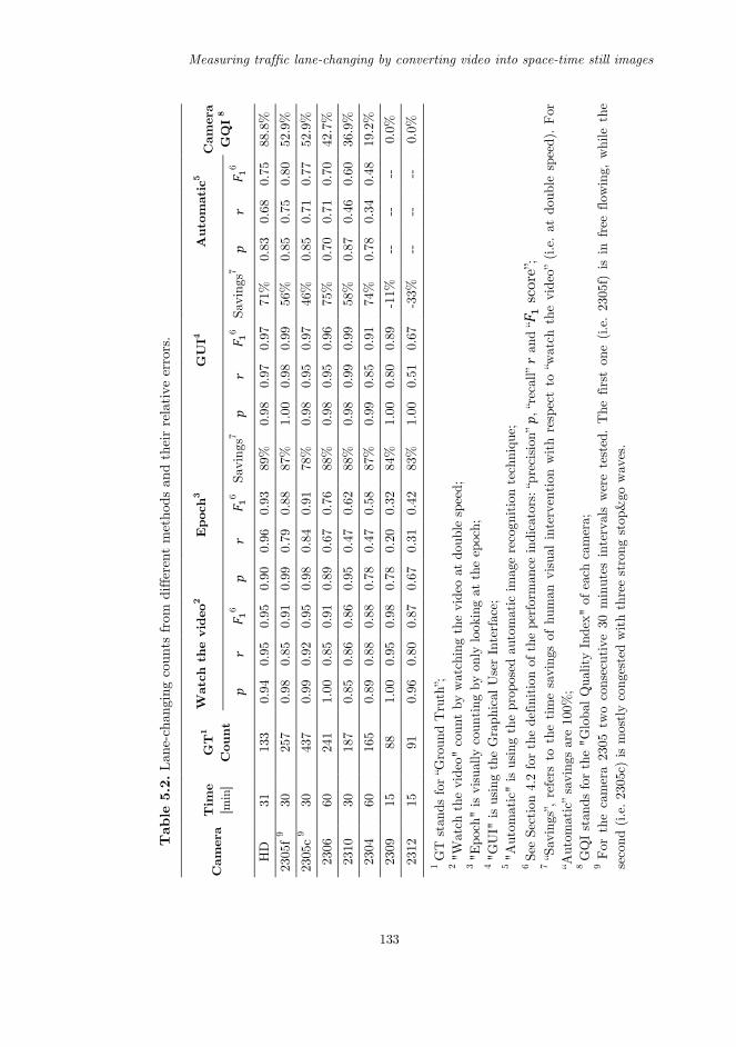
Measuring traffic lane-changing by converting video into space-time still images

133 

Tab

le 5

.2. L

ane-

chan

ging

cou

nts

from

diff

eren

t m

etho

ds a

nd t

heir

rel

ativ

e er

rors

.

Cam

era

GQ

I 8

88.8

%

52.9

%

52.9

%

42.7

%

36.9

%

19.2

%

0.0%

0.0%

1 G

T s

tand

s fo

r “G

roun

d T

ruth

”; 2 "W

atch

the

vid

eo"

coun

t by

wat

chin

g th

e vi

deo

at d

oubl

e sp

eed;

3 "E

poch

" is

vis

ually

cou

ntin

g by

onl

y lo

okin

g at

the

epo

ch;

4 "G

UI"

is u

sing

the

Gra

phic

al U

ser

Inte

rfac

e;

5 "A

utom

atic

" is

usi

ng t

he p

ropo

sed

auto

mat

ic im

age

reco

gnitio

n te

chni

que;

6 Se

e Se

ctio

n 4.

2 fo

r th

e de

finitio

n of

the

per

form

ance

indi

cato

rs: “

prec

isio

n” 𝑝

, “re

call”

𝑟 a

nd “

𝐹 s

core

”; 7

“Sav

ings

”, re

fers

to

the

tim

e sa

ving

s of

hum

an v

isua

l in

terv

ention

with

resp

ect

to “

wat

ch t

he v

ideo

” (i.e

. at

dou

ble

spee

d).

For

“A

utom

atic

” sa

ving

s ar

e 10

0%;

8 G

QI

stan

ds fo

r th

e "G

loba

l Qua

lity

Inde

x" o

f eac

h ca

mer

a;

9 For

the

cam

era

2305

tw

o co

nsec

utiv

e 30

min

utes

int

erva

ls w

ere

test

ed.

The

fir

st o

ne (

i.e.

2305

f) i

s in

fre

e flo

win

g, w

hile

the

se

cond

(i.e

. 230

5c)

is m

ostly

cong

este

d w

ith

thre

e st

rong

sto

p&go

wav

es.

Aut

omat

ic5 𝐹

6

0.75

0.

80

0.77

0.

70

0.60

0.

48

--

--

𝑟 0.68

0.

75

0.71

0.

71

0.46

0.

34

--

--

𝑝 0.83

0.

85

0.85

0.

70

0.87

0.

78

--

--

GU

I4

Savi

ngs7

71%

56

%

46%

75

%

58%

74

%

-11%

-33%

𝐹6

0.97

0.

99

0.97

0.

96

0.99

0.

91

0.89

0.67

𝑟 0.97

0.

98

0.95

0.

95

0.99

0.

85

0.80

0.51

𝑝 0.98

1.

00

0.98

0.

98

0.98

0.

99

1.00

1.00

Epo

ch3

Savi

ngs7

89%

87

%

78%

88

%

88%

87

%

84%

83%

𝐹6

0.93

0.

88

0.91

0.

76

0.62

0.

58

0.32

0.42

𝑟 0.96

0.

79

0.84

0.

67

0.47

0.

47

0.20

0.31

𝑝 0.90

0.

99

0.98

0.

89

0.95

0.

78

0.78

0.67

Wat

ch t

he v

ideo

2

𝐹6

0.95

0.

91

0.95

0.

91

0.86

0.

88

0.98

0.87

𝑟 0.95

0.

85

0.92

0.

85

0.86

0.

88

0.95

0.80

𝑝 0.94

0.

98

0.99

1.

00

0.85

0.

89

1.00

0.96

GT

1 C

ount

133

257

437

241

187

165

88

91

Tim

e [m

in]

31

30

30

60

30

60

15

15

Cam

era

HD

23

05f 9

2305

c 9

2306

23

10

2304

23

09

2312

 

Chapter V 

134 

Using the GUI allows a better interpretation of the epoch, bringing clear benefits in terms of accuracy. In most of the cameras the GUI outperforms the “watching the video” method in terms of accuracy, investing less than half of the visual processing time. It has been found that when two lane changes happen at different locations but almost at the same time, only one is generally detected by watching video1. In contrast, using the GUI both can be clearly identified, leading to a significantly better count when a lot of activity happens. In conclusion, the GUI is an accurate and fast method if the recording fulfills a minimum quality (i.e. GQI >20% Otherwise, if the quality of the recording is extremely poor, the GUI does not help, either in reducing the visual processing time, or in achieving higher accuracies with respect to watching the video. Cameras 2309 and 2312 are an example of this undesirable situation.

Regarding the fully automatic procedure, a lower accuracy is the price one has to pay in order to avoid completely the visual intervention. The implemented machine learning algorithm does not improve the performance of the human analyst in the identification of lane changes from the epoch, and the obtained accuracy is in general worse, with values of 𝐹 0.80, at best. In addition, the accuracy of the results rapidly deteriorate with the reduction of the quality of the recording, so that, if the quality of the recording is not good (i.e. GQI >40%) results cannot be considered reliable (i.e. 𝑝 or 𝑟 below 0.5). The effects of the length of the training sample on the accuracy of the method have also been analyzed (see Figure 5.8). Results show that longer training samples slightly improve accuracy when the default accuracy of the automatic method is very bad, because of an insufficient quality of the recording. In contrast, if the default accuracy is already on its higher levels, extending the training sample does not contribute in further improvements. In conclusion, if the quality of the recording is good, the minimum training sample (e.g. 50 lane changes) suffices.

Results in Table 5.2 also show that the accuracy of the methods is not significantly affected by different traffic regimes (i.e. free-flowing or congested). This can be seen by comparing the results in Camera 2305f and 2305c.

                                                             

1 Three different analysts suffered this problem, and all of them agreed that it is intrinsic to the "watching the video" method.

Measuring traffic lane-changing by converting video into space-time still images

135 

Figure 5.8: Evolution of error in the automatic method for different training sample sizes.

Figure 5.9: Evolution of error with the quality of the recording. Note: Tendency lines are obtained from least squares regression to data.

Figure 5.10: Detailed video quality indicators and resulting 𝐹 accuracy metric. Note: 𝑞 and 𝑞 are not displayed since they are 100% for all cameras. GQI stands for the Global quality index.

Chapter V 

136 

Given the previous results, it is interesting to compare the different sensitivities of the analyzed methods with respect to the quality of the recordings. On the one hand, watching the video results in accuracy levels around 𝐹 0.9 on average, and this is almost insensitive to the quality of the recording. On the other hand, the accuracy of all the other methods, based on the epoch, is strongly dependent on the global quality index. In these methods, accuracy increases with the quality of the recordings. Figure 5.9 illustrates these facts, and could be used to support the selection of the video processing technique, given the global quality index of the recording and the required accuracy of the results.

Further detail is provided in Figure 5.10, which shows the effects of each

individual factor (i.e. 𝑞 ; 𝑖 1 6; see Table 5.1 and Appendix 2) in the global quality index and eventually in the accuracy level, 𝐹 . From Figure 5.10 it can be concluded that a poor performance in one particular quality indicator cannot be compensated by better results in other indicators. For instance, poor image quality (i.e. brightness – 𝑞 , clipping – 𝑞 , or contrast – 𝑞 ) is not compensated by a better image framing (scanline alignment – 𝑞 , length – 𝑞 , or resolution – 𝑞 ) or vice versa. So, all individual quality factors need to be considered when setting up the video cameras for the experiment. These evidences support the multiplicative structure of the global quality index (see Appendix 2) and lead to the recommendations for the camera settings provided in Section 3.4.

4.3. Findings from the measured lane-changing data

To illustrate the applicability of the lane-changing data obtained using the proposed semi-automatic methodology (GUI method), the results of a preliminary traffic analysis are presented here. For instance, the data extracted from the video recordings allow empirically proving that the lane-changing rate peaks during traffic state transitions (i.e. from free flowing to congestion, or vice versa).

This can be seen in Figure 5.11, where oblique cumulative count (N-curve), cumulative occupancy (T-curve), and cumulative lane-changing (L-curve) with respect to time are plotted. Using these curves, the transition between free flow and congestion is identified by an increase of the occupancy (slope of the T-curve) simultaneously with a decrease of the flow (slope of the N-curve). This happens slightly before 8:30 in Figure 5.11. In turn, the recovery of free flowing conditions is identified by an occupancy

Measuring traffic lane-changing by converting video into space-time still images

137 

drop (i.e. around 9:00 in Figure 5.11). It can be seen that in both situations, the lane changing rate peaks (slope of the L-Curve).  

Figure 5.11: Oblique cumulative count (N), occupancy (T) and lane-changing (L) curves. Note: Lane-changing data from camera 2306; Flow and occupancy data are measured by a loop detector on the same freeway segment; The subtracted background flow is 95% of the average. See (Cassidy and Windover, 1995) for a detailed description of the oblique cumulative count method. Furthermore, the perspective correction method developed in this paper

allows locating the lane changes in their real position on the freeway. Figure 5.12 illustrates the spatial distribution of the lane-changing data, and shows how the solid line, between the central and shoulder lanes, reduces lane-changing rates. Also, just after the end of the solid line, the void left by vehicles exiting at the off-ramp produces an increase of the lane-changing rates in this area.

Figure 5.12: Location of lane changes. Note: Data from camera 2305; Traffic goes from left to right; A solid line on the pavement bans lane-changing from the middle to the shoulder lane at the off-ramp location.

Chapter V 

138 

While lane-changing is a complex drivers’ decision process and further

research would be needed to model the phenomenon, this simple analysis only pretends to show interesting research directions supported by the data obtained with the proposed methodology. In addition, the application of the proposed method could allow other “microscopic” applications. For instance, the perspective correction method could be used to determine the duration in time and space of each lane change maneuver, by analyzing the shape of the “stain” on the epoch. This would open up new research directions.

5. Conclusions

On the one hand, visually extracting traffic data from video recordings requires multiple visualizations. This task is time consuming and extremely tedious. On the other hand, for relatively short applications like the ones in a research context, full automatic methods are over-complicated, costly and do not provide the required accuracy. In between semi-automatic methods do have an opportunity. They are simple video processing tools, aimed to ease and speed up the visual process without falling in the complexities and inaccuracies of complete automation.

The proposed semi-automatic method is based on the transformation of the video recordings, obtained from a fixed camera, to an adequate standstill image, called "epoch", from were to visually identify lane changes. The method, which has been implemented on a user friendly GUI, speeds-up the completely visual procedure by concentrating human intervention only on the time windows where some activity happens. For the sake of comparison in the accuracy of the results, the visual identification of lane changes from the epochs has been automated using a machine learning algorithm, achieving a fully automated tool in this case.

The proposed semi-automatic method was to be applied to 63 hours of recordings from 7 cameras on a Spanish freeway. 2 of these cameras did not meet the minimum recording quality in order to apply the method with reliability. This left "only" 45 hours to process. Using the typical visual procedure, the extraction of the lane-changing data from the videos would have taken 50 hours of labor, as the video needs to be watched once for every pair of lanes at a maximum of double speed (note that sections with 3 and 4 lanes were analyzed). In contrast, it took only 7 hours by using the GUI, resulting in 43 hours of labor saved (i.e. 86% of "visual" processing

Measuring traffic lane-changing by converting video into space-time still images

139 

time saved). In addition, this has been achieved with an increased accuracy in the lane change count and providing the precise time and location of the lane changes, which is not common in visual methods.

Regarding the accuracy of the methods (in terms of the 𝐹 score), while the completely visual procedure leads to accuracy levels of 0.86 0.98 for different cameras, by using the GUI semi-automatic method this accuracy is always above 0.95, provided that the recording meets some minimum quality standards (i.e. minimum of 35% in the developed global quality index - GQI - out of 100% for an optimal recording). Also, for recordings with a rather poor quality (e.g. GQI = 20%) the accuracy drops only to 0.90, still above the results achieved with the visual procedure (i.e. 0.88 for this quality of recording). In spite of this, the recommendations regarding the video quality and framing are crucial in order to successfully use the method. The better the video quality, the easier, faster and more reliable the counting. It should also be noted that an extremely poor quality of the recordings (i.e. GQI = 0%) invalidates the reliable use of the semi-automatic method, leaving the visual procedure as the only alternative.

Regarding the fully automated implementation of the method, two conclusions are obtained. First, the accuracy of the results deteriorates, as expected, with 𝐹 values around 0.80 in the best cases. Second, the accuracy of the results depends much more strongly on the quality of the recordings, so that, for recordings with GQI < 40%, a reliable count cannot be obtained. Therefore, automatic methods should only be applied when the quality of the recordings is high and low precision data suffices.

Finally, it has also been found that both, the semi-automatic and the fully automatic methods, perform equally well (or equally bad) in free-flowing and in congested traffic regimes.

It remains as further research the application of the method to stable aerial footage, with the benefits of reduced perspective issues and without occlusions. Also, the method could be adapted to be used with recordings taken from a probe vehicle, exploding the benefits of a moving observer in relating the lane-changing behavior with the properties of the traffic flow.

6. Acknowledgements

Authors acknowledge the collaboration of the Servei Català de Trànsit, the Catalan traffic administration for the provision of the required video recordings. The work of Adrià Torres in the counting of lane changes and his

Chapter V 

140 

feedback is also gratefully acknowledged. This research has been partially funded by the Spanish Ministry of Science and Innovation (TRA2016-79019-R/COOP).

Appendix 1

Video recordings suffer from perspective deformation and distortion. This Appendix 1 presents the assessment of the effects of distortion together with an analytical method to correct perspective deformation. Table 5.A1 summarizes the variables and parameters involved. Figures 5.A1 and 5.A2 provide their graphical definition.

A1.1 Effects of distortion on a flat sensor

Figure 5.A3 illustrates the effects of distortion, considering a camera with a distance 𝑟 between the flat sensor and the focal point. In the theoretical ideal curved sensor, the ray of width 𝜕𝛾 encompasses the same number of pixels for all 𝛾 values. In contrast, in the real flat sensor, the number of pixels encompassed by 𝜕𝛾 depends on 𝛾, being maximum for 𝛾 𝐹𝑂𝑉/2 and minimum for 𝛾 0. This effect is known as image distortion.

 

Figure 5.A1: Graphical definition of parameters. From Figure 5.A3 it can be seen that 𝑥 𝑟 tan 𝛾 , while 𝑥 𝑟 𝛾.

Then, the increase in 𝑥 and 𝑥 when 𝛾 increases by 𝜕𝛾, is it expressed by the derivatives 𝑥 and 𝑥 , as computed in Equations 5.A1 and

𝑑 𝑑

𝜃

𝛼

𝛼

Camera

Road 𝑑

ℎ ℎ

𝐹𝑂𝑉

Vertical

Horizontal

𝑑

Measuring traffic lane-changing by converting video into space-time still images

141 

5.A2. Equation 5.A2 shows that in the ideal sensor this magnitude is constant and does not depend on 𝛾.

Table 5.A1. Definition of variables and parameters in the perspective correction method. Note: *"Value" stands for the particular application to the HD camera (see Figure 5.2).

Var. Units Description 𝛼 [rad] Angle between the ray of vision and the orthogonal to the road

𝑑 [m] Straight distance from the base of the camera to the point where the ray of vision reaches the road

𝛾 [rad] Angle between the bisector of the field of view (𝐹𝑂𝑉) and the ray of vision;

𝛾 𝛼 𝛼 𝛼 2⁄ 𝜕𝛾 [rad] Differential of 𝐹𝑂𝑉.

Par. Units Value* Description

𝐹𝑂𝑉 [rad] 0.106 Field Of View (total angle of vision of the camera framing).

𝛼 𝛼

[rad] 1.431 1.537

Angle between the lower 𝛼 or upper 𝛼 ray of vision and the orthogonal to the road; 𝛼 𝛼 𝛼 ; 𝛼 𝛼 𝐹𝑂𝑉

ℎ [m] 8 Camera height from the base. 𝑑 [m] 179 Length of the scanline on the road.

𝑑 [m] 178.2 Length of the scanline projection on the camera 𝐹𝑂𝑉 plane. 𝑑 𝑑 .

𝑑 𝑑

[m] 57 235

Straight distance from the base of the camera to nearest 𝑑 or furthest 𝑑 point where the 𝐹𝑂𝑉 reaches the road; 𝑑 𝑑 𝑑 ; 𝑑 𝑑 𝑑

𝜃 [rad] 4.01·10-2 Slope of the road with respect to the horizontal.

𝜕𝛼 [rad / pixel]

5.54·10-5 Angular value of one pixel in the original scanline

𝑣 [m/s] 22.22 Traffic free-flow speed 𝑓𝑝𝑠 [fps] 50 Video frames per second.

𝑔 [pixels/ frame]

1 Perspective correction factor

𝑚 [pixels] 1226 Number of vertical pixels in the original epoch.

𝑛 [pixels] 403 Number of vertical pixels in the perspective corrected epoch.

 

Chapter V 

142 

 

Figure 5.A3: Distortion effects on a flat sensor.

𝑥 𝑟 1 tan 𝛾 (5.A1)

𝑥 𝑟 (5.A2) Distortion, 𝑒 , is expressed as the relative difference between 𝑥 and 𝑥

(i.e. the differential error), which depends on 𝛾, as expressed in Equation 5.A3. The average error for a given 𝐹𝑂𝑉 is computed as the integral of Equation 5.A3 over the whole range of 𝛾.

𝑒 𝛾𝑥 𝑥

𝑥 tan 𝛾 (5.A3)

 

Figure 5.A3: Maximum and average distortion values for different 𝐹𝑂𝑉s on a flat sensor. Note: The values of the 𝐹𝑂𝑉 have been limited to 𝜋/4 as wider 𝐹𝑂𝑉s have little sense for this application. Figure 5.A3 shows average and maximum distortion as a function of

different 𝐹𝑂𝑉s. Because small 𝐹𝑂𝑉s are recommended for this application,

 

 𝛾

Focal Point

Real flat sensor Ideal curved sensor

𝐹𝑂𝑉

𝑥 𝑥

𝑟

𝜕𝛾

Vertical

Horizontal 𝑚

Measuring traffic lane-changing by converting video into space-time still images

143 

the effects of distortion are small and can be neglected. For the case study presented in Section 4, the maximum 𝐹𝑂𝑉 is 0.27 rad, resulting in an average and maximum distortion of 0.08% and 1.87% of the pixel size respectively.

A1.2 The perspective corrected scanline

Perspective deformation happens because as 𝛼 increases (i.e. more distant view) a larger stretch of freeway is seen within a constant 𝜕𝛼. In order to develop a simple correction method for the perspective deformation, two assumptions are made: i) no camera distortion (i.e. ideal curved sensor), and ii) a constant grade of the road, 𝜃. These assumptions approximately hold for the present application, because distortion can be neglected for small 𝐹𝑂𝑉s, and road grades are smooth in the relatively small distances of the scanline.

Equation 5.A4 is derived from the geometry in Figure 5.A1, and allows computing 𝑑, the distance from the base of the camera to any point seen with an angle 𝛼. In turn, Equation 5.A5 computes the rate of change of this distance for an incremental change in 𝛼.

𝑑 ℎ tan 𝛼 𝑑 (5.A4)

𝑑𝜕 𝑑

𝜕𝛼 ℎ 1 tan 𝛼 (5.A5)

Where ℎ ℎ cos 𝜃 and 𝑑 ℎ sin 𝜃 .

Because distortion effects are neglected, it can be assumed that all pixels in the scanline represent a constant 𝜕𝛼. So, using linear interpolation, it is possible to construct a vector identifying the α ’s for all the pixels in the original scanline, where 𝑖 ∈ 1 𝑚, being 𝑚 the number of pixels in the original scanline. Note that under these assumptions, 𝜕𝛼 𝛼 𝛼 𝑚⁄ . Then, using Equation 5.A5, the distance corresponding to the α pixel in the original scanline is computed as 𝑑 𝑓 𝑑 ∂𝛼, where 𝑓 is a correction factor to take into account that the total distance of the scanline projection on the 𝐹𝑂𝑉 plane is smaller than the real one.

This is:

𝑑 𝜕𝛼 𝑑 𝑑 (5.A6)

Chapter V 

144 

The inequality in Equation 5.A6 turns to equality only in case of a

straight scanline with a parallel camera alignment (𝐹𝑂𝑉). In other cases d d . So, the correction factor, 𝑓, defined in Equation 5.A7, needs to be applied in order to obtain the real world distance represented by each pixel.

𝑓𝑑𝑑

(5.A7)

Recall that the objective of perspective correction is that each pixel in

the corrected scanline covers the same real world distance. This distance can be expressed as 𝑑 𝑛⁄ , where 𝑛 is the number of pixels in the corrected scanline. While 𝑛 can be an arbitrarily selected integer, in order to obtain epochs where lane changes are clearly identified by vehicle shaped stains over the pavement background, it is recommended for 𝑛 to be at least the number of frames taken by a vehicle to travel the whole scanline length at free-flow speed. This is:

𝑛 𝑔𝑑𝑣

𝑓𝑝𝑠 (5.A8)

Where 𝑔 1 is a user defined perspective correction parameter. The

larger 𝑔, the higher the epoch, but the more deformed the vehicular shape in the epoch.

Given the real world distance encompassed by each pixel in the original scanline 𝑑 , which is a function of α ∀𝑖 1 𝑚, and the constant real world distance to be covered by pixels in the corrected version of the scanline, 𝑑 𝑛⁄ , the perspective correction algorithm works as follows:

If 𝑑 𝑑 𝑛⁄ , the density of pixels per unit length in the original scanline is too high and some pixels need to be skipped in the corrected epoch

If 𝑑 𝑑 𝑛⁄ , the density of pixels per unit length in the original scanline is too low and some pixels need to be replicated. This situation, which happens in the furthest part of the scanline (especially if the 𝐹𝑂𝑉 is large) is undesirable because it implies lack of information and results in blurry parts of the epoch. For the recommended small 𝐹𝑂𝑉s, the worst pixel on the original scanline with the largest 𝑑 might need to be replicated up to 4 times.

The algorithm in Figure 5.A4 summarizes the method.

Measuring traffic lane-changing by converting video into space-time still images

145 

Inputs: The 𝑚 pixels of the original scanline and their α 's ∀𝑖 1 𝑚

𝑑 𝑛⁄ 𝑑 𝑓 𝑑 ∂𝛼

Outputs: The 𝑛 pixels of the perspective corrected scanline

1 𝑐𝑜𝑢𝑛𝑡 0 2 𝒇𝒐𝒓 𝑎𝑙𝑙 𝑖 1 𝑚 3 𝑐𝑜𝑢𝑛𝑡 𝑐𝑜𝑢𝑛𝑡 𝑑 4 𝒘𝒉𝒊𝒍𝒆 𝑐𝑜𝑢𝑛𝑡 0.5 𝑑 𝑛⁄ 5 𝑎𝑑𝑑 𝑡ℎ𝑒 𝑝𝑖𝑥𝑒𝑙 𝑖 𝑡𝑜 𝑡ℎ𝑒 𝑐𝑜𝑟𝑟𝑒𝑐𝑡𝑒𝑑 𝑠𝑐𝑎𝑛𝑙𝑖𝑛𝑒 6 𝑐𝑜𝑢𝑛𝑡 𝑐𝑜𝑢𝑛𝑡 𝑑 𝑛⁄ 7 𝒆𝒏𝒅 8 𝒆𝒏𝒅

Figure 5.A4: Algorithm for the pixel selection in the perspective corrected scanline. Note: 𝑐𝑜𝑢𝑛𝑡 represents the part of the distance of the pixel in the corrected scanline covered at each iteration.

Appendix 2

An ad-hoc recording global quality index is developed in this Appendix 2. The index includes 6 different quality parameters: three for video quality (i.e. brightness, clipping and contrast.) and three devoted to the epoch framing (i.e. scanline alignment, coverage and number of unique pixels).

A2.1 Video image quality indexes

The proposed three quality indexes of the recording are based on its luminance histogram, which represents the frequency of a given luminance value in an image. The normalized cumulative luminance curve, 𝐿, is defined as the cumulative sum of the histogram divided by its total value, as expressed in Equation 5.A9.

𝐿 𝑖∑ ℎ

∑ ℎ (5.A9)

Where ℎ 𝑖 is the frequency of a given luminance bin 𝑖. 𝑖 ∈ 1, 𝑙 , ordered from darker to brighter levels, and 𝑙 is the number of different luminance values in the image. Note that a typical 8 bit image or video includes a total of 256 possible different values (i.e. 𝑙 256 . Note that 𝐿 is a monotonically increasing function and 𝐿 𝑖 ∈ 0,1 .

Chapter V 

146 

Table 5.A2. Video quality indexes and their lower and upper bound thresholds: 𝑞 _ , 𝑞 _ . Note: 𝑑 is the real length of the scanline; 𝑣 is the free-flow speed of traffic; 𝑔 is the perspective correction factor.

Indicator Definition 𝒒𝒋_𝒍 𝒒𝒋_𝒖

𝑞 1 𝐿 𝑖 𝑙4

𝑙3

𝑞 𝐿 𝑙 16 0.8 0.9

𝑞

𝑏 𝑎 Where:

𝑎 𝑀𝑖𝑛 𝑎 / 𝐿 𝑎 0,1 𝑏 𝑀𝑖𝑛 𝑏 / 𝐿 𝑏 0,9

𝑙4

𝑙2

𝑞 𝛽∑ 𝑝 𝛽

∑ 𝑝

1𝑚

-30º -5º

𝑞 𝑑𝑣

2 s 10 s

𝑞 𝑈𝑛𝑖𝑞𝑢𝑒 𝑝𝑖𝑥𝑒𝑙𝑠 25 𝑔 250·𝑔 Table 5.A2 summarizes the formulas to obtain 𝑞 , 𝑞 , and 𝑞 , the three

image quality indexes. 𝑞 addresses brightness and it is computed as the sum of the first half of the cumulative luminance curve. 𝑞 will be higher for darker images. 𝑞 assesses the highlights clipping of the image and looks for overexposed areas. 𝑞 is smaller when there are larger overexposed areas in the image (i.e. higher percentage of luminance in the brightest 16 bins). Finally, 𝑞 assesses the contrast of the image by computing the number of bins encompassing 80% of the cumulative luminance. The larger this luminance range, the better the image contrast.

Because 𝑞 , 𝑞 and 𝑞 are related to image quality, and a video is a succession of images, the quality indicator needs to be applied to a sample of frames. One frame every minute of video is considered. The quality indicator is then computed as the average of the values obtained in the sample.

A2.2 Video framing quality indexes

In Table 5.A2, 𝑞 , 𝑞 , and 𝑞 , are the three quality indexes devoted to the quality of the video framing. 𝑞 addresses the alignment of the scanline, and it is computed as the average angle, 𝛽, between the scanline and the 𝐹𝑂𝑉 plane (i.e. the vertical in the video frame). The lower 𝛽, the better the alignment. If the scanline is defined as piecewise linear, 𝛽 is easily computed

Measuring traffic lane-changing by converting video into space-time still images

147 

as a weighted average of the angle, 𝛽 , exhibited by each one of the 𝑘 parts of the scanline, where the weights are their respective length in pixels, 𝑝 . In addition, a correction factor, 𝑚 , is included in 𝑞 . In general, 𝑚 1, unless the camera is located over the freeway median. In such case 𝑚 1.25 and the misalignment is less penalizing. This is because the light vehicles in the median lane are less likely to occlude the scanlines.

𝑞 refers to the free flow travel time required to travel the whole scanline length. The longer this time, the better the framing, because the relative effect of the boundaries is reduced and more lane changes can be counted.

Finally, 𝑞 takes into account the number of unique pixels that compose the perspective corrected scanline. Recall that, in the corrected scanline, in the furthest zones of the epoch some pixels may be repeated. This happens when either the recording has a high 𝐹𝑂𝑉 and/or a small resolution. Even if the epochs are not corrected this amount of "unique pixels" is a good indicator of the framing quality, taking into account the scanline free-flow travel time, the number of frames per second, the video resolution and the perspective deformation.

A2.3 The global quality index (GQI)

The global quality index, 𝐺𝑄𝐼, is obtained as the harmonic average of the normalized versions, 𝑞 , of the previous six partial components. This is 𝑞 ∈ 0,1 ; 𝑗 1 6. In order to normalize the partial quality indexes, upper and lower bound thresholds are defined (i.e. 𝑞 _ ; 𝑞 _ ) and linear interpolation is used in between (see Equation 5.A10). Finally, the global quality index is computed as the weighted harmonic average represented in Equation 5.A11. Framing quality has a stronger impact than image quality in the global quality of the recording for this specific lane-changing monitoring application.

𝑞 max 0, min 1,𝑞 𝑞 _

𝑞 _ 𝑞 _; 𝑗 1 6 (5.A10)

GQI 𝑞 𝑞 𝑞 𝑞 𝑞 𝑞 (5.A11)

Table 5.A3 shows the results of the application of the video quality

indexes to the 7 cameras used in the present paper (see Figure 5.6).

Chapter V 

148 

Table 5.A3. Video quality indexes applied to the cameras used in the pilot test.

Camera 𝒒𝟑 𝒒𝟒 𝒒𝟓 𝒒𝟔 𝑮𝑸𝑰 HD 73.6% 90.4% 76.3% 100.0% 88.8% 2305 43.9% 28.4% 100.0% 36.2% 52.9% 2306 17.1% 33.3% 45.3% 39.6% 42.7% 2310 62.6% 58.0% 25.6% 14.5% 36.9% 2304 69.8% 42.8% 16.6% 2.1% 19.2% 2309 5.4% 0.0% 11.0% 1.6% 0.0% 2312 0.5% 0.0% 61.3% 34.6% 0.0%

Appendix 3

This Appendix 3 describes the fully automatic method implemented for detecting lane changes from the epochs. Lane changes appear in the epochs as regions with shapes, colors and geometric characteristics that are very different from the pavement background. The automatic method analyses the image to find distinctive areas that differ from the background, characterizes these regions in terms of visual descriptors and decides if they correspond to a lane change or not using a binary classifier.

A3.1 Image preprocessing and candidate extraction

The epoch (i.e. a color image; see Figure 5.A5.a) is first converted to a gray-scale image 𝑔 of size ℎ 𝑤 (ℎ height, 𝑤 width) in units of pixels. Next, an estimate of the background is obtained by computing a column vector 𝑏 of size ℎ 1, where each element 𝑖 in 𝑏 is the median of the pixel values in the corresponding row in 𝑔: 𝑏 𝑖 𝑚𝑒𝑑𝑖𝑎𝑛 𝑔 𝑖, 𝑗 . The image background (i.e. the pavement) is eliminated by subtracting the vector of median values from each image column 𝑔 𝑖, 𝑗 𝑔 𝑖, 𝑗 𝑏 𝑖 , ∀𝑖, 𝑗 (see Figure 5.A5.b). A morphological closing filter is used to connect small regions corresponding to the same component of the image that may be disconnected after removing the background.

The following step is the candidate extraction process, using a segmentation technique called Maximally Stable Extreme Regions (MSER) (Matas et al., 2002). The objective is to detect image regions that may correspond to lane changes. This algorithm finds homogeneous components of high contrast with respect to the surrounding area. Finally, post-processing morphological filters are applied to fill holes, remove thin leakages

Measuring traffic lane-changing by converting video into space-time still images

149 

and filter out small regions. Figure 5.A5.c shows the result of this process, where white areas correspond to candidate regions. Figure 5.A5.d presents these regions filled with the original image values (pixel-wise product between the epoch A5.a and the binary mask A5.c).

A3.2 Classification

(a) Original epoch

(b) Background subtraction 𝑔

(c) Candidate region mask

(d) Final candidate regions

(e) Classification result. True positive and true negative regions are depicted with red and magenta dots, respectively, while green dots correspond to ground truth lane changes

Figure 5.A5: Automatic epoch processing for lane change detection. After the preprocessing stage, a set of candidate regions is obtained. A

binary classifier is then used to discriminate between positive (i.e. lane change) and negative (i.e. occlusion, shade or other artifacts) regions.

The classification is done with a Support Vector Machine (SVM) model. The classifier hyperparameters (width of the Gaussian kernel and regularization parameter) are selected by cross-validation, minimizing the 𝐹

Chapter V 

150 

measure. The features used by the classifier are: area of the region, region orientation, mean value of each color component in the region (using the YCbCr color space), histogram in each color component, horizontal and vertical projections of the region mask, and lower and upper limits of the region bounding box. The same set of features is used in all the experiments (i.e. for all cameras).

One classifier is trained for each camera. The data used to train each SVM is obtained applying the preprocessing and region extraction procedures to epochs computed from a portion of the video and using annotations from the GUI to label each region as positive or negative. It is important to note that the classifiers are not trained using real ground truth labels but noisy labels provided by the GUI, as would be the case in real practice. This issue might have a negative impact on the accuracy metrics reported for the fully automatic method. Following the example, Figure 5.A5.e presents the classification results.

References

Adeli, H. and Karim, A. (2005). Wavelets in intelligent transportation systems. John Wiley and Sons, New York.

Angel, A., Hickman, M., Mirchandani, P., and Chandnani, D. (2003). Methods of analyzing traffic imagery collected from aerial platforms. IEEE Transactions on Intelligent Transportation Systems, 4(2), 99–107.

Alireza, A., Karami-Mollaie, M., and Baleghi Y. (2012). Object tracking using adaptive object color modelling. In: Proceeding of 4th Conference on Information and Knowledge Technology, 848-852.

Avery, R., Wang, Y., and Zhang, G. (2007). Video-based vehicle detection and classification system for real-time traffic data collection using uncalibrated video cameras. Transportation Research Record, 1993(1), 138–147.

Bhaskar, P.K., and Yong, S.P. (2014). Image processing based vehicle detection and tracking method. In: IEEE 2014 International Conference on Computer and Information Sciences, (ICCOINS), Kuala Lumpur, 1-5.

Buisson, C., Villegas, D., and Rivoirard, P. (2016). Using polar coordinates to filter trajectories data without adding extra physical constraints. In: Proceedings of the 95th Annual Meeting of the Transportation Research Board, Washington D.C.

Measuring traffic lane-changing by converting video into space-time still images

151 

Campbell, R. (2012). An analysis framework for evaluation of traffic compliance measures. PhD thesis. University of California, Berkeley.

Campbell, R., and Skabardonis, A. (2013). Analysis framework for evaluation of traffic compliance measures. Transportation Research Record, 2364, 71–79.

Canny, J. (1986). A computational approach to edge detection. IEEE Transactions on Pattern Analysis and Machine Intelligence, 8(6), 679–698.

Cassidy, M.J., and Windover, J. (1995). Methodology for assessing dynamics of freeway traffic flow. Transportation Research Record, 1484, 73–79.

Cassidy, M.J., Jang, K., and Daganzo, C.F. (2010). The smoothing effect of carpool lanes on freeway bottlenecks. Transportation Research A, 44(2), 65–75.

Cheung, S.C.S., and Kamath, C. (2005). Robust background subtraction with foreground validation for urban traffic video. Eurasip Journal on Applied Signal Processing, 2005(14), 2330–2340.

Coifman, B., Beymer, D., McLauchlan, P., and Malik, J. (1998). A real-time computer vision system for vehicle tracking and traffic surveillance. Transportation Research Part C, 6(4), 271–288.

Coifman, B., Mishalani, R., Wang, C., and Krishnamurthy, S. (2006). Impact of lane-change maneuvers on congested freeway segment delays: Pilot study. Transportation Research Record, 1965, 152–159.

Coifman, B. and Li, L. (2017). A critical evaluation of the Next Generation Simulation (NGSIM) vehicle trajectory dataset. Transportation Research Part B 105, 362–377.

Duret, A., Ahn, S., and Buisson, C. (2011). Passing rates to measure relaxation and impact of lane-changing in congestion. Computer-Aided Civil and Infrastructure Engineering, 26(4), 285–297.

Federal Highway Administration. (2006). Interstate 80 Freeway Dataset Factsheet.

Federal Highway Administration. (2015). Next Generation Simulation (NGSIM). Retrieved March 3, 2016, from: http://ops.fhwa.dot.gov/trafficanalysistools/ngsim.htm

Chapter V 

152 

Ghosh-Dastidar, S., and Adeli, H. (2003). Wavelet-clustering -neural network model for freeway incident detection. Computer-Aided Civil and Infrastructure Engineering, 18(5), 325-338.

Karim, A., and Adeli, H. (2003). Fast automatic incident detection on urban and rural freeways using wavelet energy algorithm. Journal of Transportation Engineering, ASCE, 129(1), 57-68.

Knoppers, P., Van Lint H., and Hoogendoorn, S. (2012) Automatic stabilization of aerial traffic images. In: Proceedings of the Transportation Research Board 91st Annual Meeting, Washington, D.C.

Kumar, P., Ranganath, S., Weimin, H., and Sengupta, K. (2005). Framework for real-time behavior interpretation from traffic video. IEEE Transactions on Intelligent Transportation Systems, 6(1), 43–53.

Laval, J., Cassidy, M.J., and Daganzo, C.F. (2007). Impacts of lane changes at merge bottlenecks: a theory and strategies to maximize capacity. In: Traffic and Granular Flow’05, Springer, Berlin, Heidelberg, 577-589.

Mak, C.L., and Fan, H.S. (2006). Single-station algorithm using video-based data for detecting expressway incidents. Computer-Aided Civil and Infrastructure Engineering, 21(2), 120–135.

Malinovskiy, Y., Zheng, J., and Wang, Y. (2009). Model-free video detection and tracking of pedestrians and bicyclists. Computer-Aided Civil and Infrastructure Engineering, 24(3), 157–168.

Masoud, O., and Papanikolopoulos, N.P. (2001). A Novel Method for Tracking and Counting Pedestrians in Real-Time Using a Single Camera. IEEE Transactions on Vehicular Technology, 50(5), 1267-1278.

Matas, J., Chum, O., Urban, M. and Pajdla, T. (2002). Robust wide baseline stereo from maximally stable extremal regions. Proceedings of British Machine Vision Conference, 384-396.

Menendez, M., and Daganzo, C.F. (2007). Effects of HOV lanes on freeway bottlenecks. Transportation Research Part B, 41(8), 809–822.

Montanino, M., Punzo, V. (2015). Trajectory data reconstruction and simulation-based validation against macroscopic traffic patterns. Transportation Research Part B, 80, 82-106.

Montanino, M., and Punzo, V. (2013a). Making NGSIM data usable for studies on traffic flow theory : a multistep method for vehicle trajectory reconstruction. Transportation Research Record, 2390, 99-111.

Measuring traffic lane-changing by converting video into space-time still images

153 

Montanino, M., and Punzo, V. (2013b). Reconstructed NGSIM data. Retrieved from www.multitude-project.eu/exchange/101.html

Morris, B., and Trivedi, M. (2006a). Robust classification and tracking of vehicles in traffic video streams. IEEE Intelligent Transportation Systems Conference, 1078–1083.

Morris, B., and Trivedi, M. (2006b). Improved vehicle classification in long traffic video by cooperating tracker and classifier modules. In: Proceedings of the IEEE International Conference on Video and Signal Based Surveillance, AVSS 2006.

Nguyen, H.T., and Smeulders, A.W. (2004). Fast occluded object tracking by a robust appearance filter. IEEE Transactions on Pattern Analysis and Machine Intelligence, 26(8), 1099–1104.

Patire, A. (2010). Observations of lane changing patterns on an uphill expressway. PhD thesis, University of California, Berkeley.

Patire, A., and Cassidy, M.J. (2011) Lane changing patterns of bane and benefit: Observations of an uphill expressway. Transportation Research Part B, 45(4), 656–666.

Punzo, V., Borzacchiello, M., and Ciuffo, B. (2011). On the assessment of vehicle trajectory data accuracy and application to the Next Generation SIMulation (NGSIM) program data. Transportation Research Part C, 19(6), 1243–1262.

Qu, X., and Wang, S. (2015). Long-distance-commuter (LDC) lane: a new concept for freeway traffic management. Computer-Aided Civil and Infrastructure Engineering, 30(10), 815–823.

Shaoqing, M., Zhengguang, L., Jun, Z., and Chen, W. (2009). Real-time vehicle classification method for multi-lanes roads. 4th IEEE Conference on Industrial Electronics and Applications, 960– 964

Soriguera, F., and Sala, M. (2014). Experimenting with dynamic speed limits on freeways. Procedia Social and Behavioral Sciences, 160, 35–44.

Stauffer, C., and Grimson, W.E.L. (1999). Adaptive background mixture models for real-time tracking. IEEE Computer Society Conference on Computer Vision and Pattern Recognition, 246-252.

Sun, D.J., and Kondyli, A. (2010). Modeling vehicle interactions during lane-changing behavior on arterial streets. Computer-Aided Civil and Infrastructure Engineering, 25(8), 557–571.

Chapter V 

154 

Sun, D.J., and Elefteriadou, L. (2012). Lane-changing behavior on urban streets: an “in-vehicle” field experiment-based study. Computer-Aided Civil and Infrastructure Engineering, 27(7), 525–542.

Tsai, Y., and Huang, Y. (2010). Automatic detection of deficient video log images using a histogram equity index and an adaptive Gaussian mixture model. Computer-Aided Civil and Infrastructure Engineering, 25(7), 479–493.

Uke, N., and Thool, R. (2013). Moving vehicle detection for measuring traffic count using OpenCV. Journal of Automation and Control Engineering, 1(4), 349–352.

Zheng, J., Wang, Y., Nihan, N.L., and Hallenbeck, M.E. (2006). Detecting cycle failures at signalized intersections using video image processing. Computer-Aided Civil and Infrastructure Engineering, 21(6), 425–435.

Zheng, Z., Zhou, G., Wang, Y., Liu, Y., Li, X., Wang, X., and Jiang, L. (2013). A novel vehicle detection method with high resolution highway aerial image. IEEE Journal of Selected Topics in Applied Earth Observations and Remote Sensing, 6(6), 2338–2343.

Chapter VI

Freeway lane-changing: some empirical findings

Published in Transportation Research Procedia 33, 2018, pp. 107-114.

157 

Freeway lane-changing: some empirical findings

Marcel Sala*a and Francesc Sorigueraa

aBarcelona Innovative Transport – UPC – Barcelona Tech, Jordi Girona 1-3, Building B1, Office 114, 08034 Barcelona, Spain.

Abstract Lane changing activity is thought to play an important role in the capacity degradation of congested freeways. However, proofs of this negative impact are scarce due to the difficulties in obtaining suitable data. In this paper, the lane changing activity in the B-23 freeway accessing the city of Barcelona is analyzed. Lane changes (LC) were video recorded in six different stretches from where loop detector measurements were also available. The obtained database allowed finding a consistent relationship between LC activity and congestion. LC peaks in all analyzed sections when they become congested. This is particularly intense at the traffic breakdown, between congested and free flowing conditions. As an example, it is observed that LC activity peaks just downstream of a fixed bottleneck where free-flowing conditions are recovered. In addition, data show that the larger the lane changing rates, the smaller the maximum observable flows, supporting the hypothesis that LC is a key contributor to a capacity drop. In spite of all these findings, this research highlights the difficulty in obtaining a suitable database to definitively answer most of the research questions regarding freeway lane-changing. The spatial coverage of measurements is one of the major drawbacks. To this end, a careful planning of the data collection is necessary in order to obtain meaningful conclusions. Keywords: Lane changing, freeway traffic, capacity drop, empircal traffic database, freeway congestion.

* Corresponding author

Chapter VI 

158 

1. Introduction

Freeway congestion is a recurrent phenomenon around the world. When demand exceeds the capacity, congestion arises. The paradox is that when traffic breaks down, the available supply (i.e. the capacity) is reduced. This harmful phenomenon is known as the capacity drop, and has been found repeatedly around the world (Banks, 1991; Hall and Agyemang-Duah, 1991; Cassidy and Bertini, 1999; Cassidy and Rudjanakanoknad, 2005; Chung et al., 2007; Patire and Cassidy, 2011; Oh and Yeo, 2012; Srivastava and Geroliminis, 2013; Yuan et al., 2015). The typical capacity drop in active freeway bottlenecks ranges from 3% to 18 % (Oh and Yeo, 2012).

While the existence of the capacity drop has been extensively demonstrated, the traffic mechanism behind it is still under debate. In the literature two traffic characteristics closely related to capacity reductions have been explored: lane changing and vehicle sluggish acceleration when leaving a queue.

Lane changing has been found to cause a capacity reduction near bottlenecks in different scenarios. In Cassidy and Rudjanakanoknad (2005) systematic lane-changing from the shoulder to faster lanes caused traffic breakdown. Patire and Cassidy (2011) found a significant flow reduction after lane-changing increases due to the existing speed variation between lanes. Also, the massive lane-changing happening at speed drops generates disturbances which end up queueing all lanes (Hatakenaka et al., 2006). In contrast, on a congested freeway, when a HOV lane is activated it smoothens traffic even in the adjacent general purpose lanes, reducing the amount of lane-changing and increasing the freeway capacity (Menendez and Daganzo, 2007; Cassidy et al., 2010).

Vehicles’ sluggish acceleration was found to be related to lane-changing in Laval and Daganzo (2006) and Leclercq et al. (2011), where lane-changing vehicles near a bottleneck were found to create larger gaps at the arriving lane due to their limited acceleration when moving from a slow to a faster lane. This leads to a total throughput reduction. These findings are in accordance with Yuan et al. (2015), where it is reported that the slower the queue speed, the greater the capacity drop.

However, the negative effects of lane-changin are not limited to being a main capacity drop contributor. Also, they trigger traffic oscillations (Mauch and Cassidy, 2002; Wang and Coifman, 2008) and stop and go waves (Ahn

Freeway lane-changing: some empirical findings

159 

and Cassidy, 2007). Moreover, lane changes are found to globally increase delay in Coifman et al. (2006), as the time saved in the exiting lane is smaller than the induced delay in the arriving lane.

In spite of all these laudable findings, the lack of reliable empirical data has been a recurrent problem to increase the knowledge on lane-changing behavior and its effects. Several researchers have designed ad-hoc experiments to validate their models (Sun and Kondyli, 2010; Sun and Elefteriadou, 2012).. In light of this data scarcity, big efforts have been made to construct reliable databases to support the research community. Take as an example the NGSIM project (FHA, 2005; FHA 2006). Unfortunately, the freeway traffic trajectories database resulting from the project, suffers from large errors regarding lateral vehicle position (Punzo et al., 2011). Thus, directly estimating lane changing from NGSIM database implies big errors. In order to correct this issue, Montanino and Punzo (2015) did a meticulous data filtering job to improve lane assignment in the NGSIM dataset. Still, some errors remain as Coifman and Li (2017) point out. This later work finds some of the error sources, like vehicles (mostly motorcycles) traveling on the hard shoulder, or in between lanes.

The present paper contributes in filling this void by exploding a comprehensive freeway traffic database obtained from a variable speed limit experiment on the B-23 freeway accessing the city of Barcelona (Soriguera and Sala, 2014). The database includes measurements from different types of traffic detectors, placed with high density on the analyzed freeway stretch. This allows a detailed characterization of flow, occupancy and average speed on the freeway. In addition, videos recorded by freeway surveillance cameras are also available for some zones, from which lane-changes are extracted by using a semi-automatic video processing method (Sala et al. 2018). This makes the database a particularly adequate and unique source of empirical data to assess freeway lane-changing behavior. Soriguera et al. (2017) analyzes several different traffic variables including lane changing in a single location. In the current paper the database has allowed providing empirical proofs to some key aspects regarding lane-changing in multiple locations, like its contribution to the capacity drop due to the peaking of lane-changing rates at traffic state transitions between congestion and free-flowing traffic.

The reminder of the paper is organized as follows. In section 2 the traffic database used to obtain some empirical findings regarding lane-changing is presented. This also includes a description of the methods used to process and aggregate the data. Section 3 presents the main findings and shows the lane-changing peaking in congestion and at bottleneck locations. How the

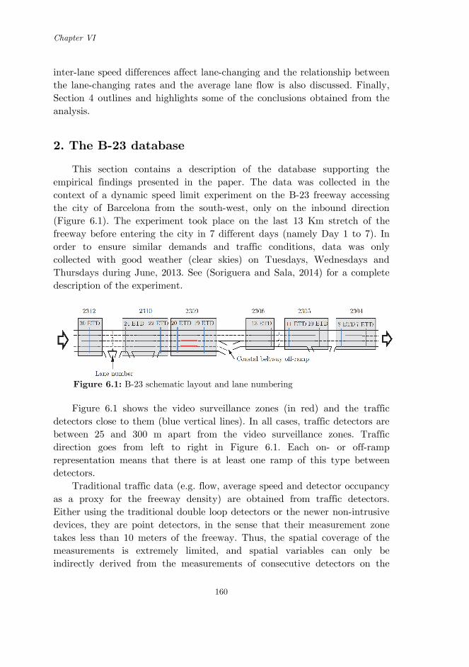
Chapter VI 

160 

inter-lane speed differences affect lane-changing and the relationship between the lane-changing rates and the average lane flow is also discussed. Finally, Section 4 outlines and highlights some of the conclusions obtained from the analysis.

2. The B-23 database

This section contains a description of the database supporting the empirical findings presented in the paper. The data was collected in the context of a dynamic speed limit experiment on the B-23 freeway accessing the city of Barcelona from the south-west, only on the inbound direction (Figure 6.1). The experiment took place on the last 13 Km stretch of the freeway before entering the city in 7 different days (namely Day 1 to 7). In order to ensure similar demands and traffic conditions, data was only collected with good weather (clear skies) on Tuesdays, Wednesdays and Thursdays during June, 2013. See (Soriguera and Sala, 2014) for a complete description of the experiment.

Figure 6.1: B-23 schematic layout and lane numbering

Figure 6.1 shows the video surveillance zones (in red) and the traffic

detectors close to them (blue vertical lines). In all cases, traffic detectors are between 25 and 300 m apart from the video surveillance zones. Traffic direction goes from left to right in Figure 6.1. Each on- or off-ramp representation means that there is at least one ramp of this type between detectors.

Traditional traffic data (e.g. flow, average speed and detector occupancy as a proxy for the freeway density) are obtained from traffic detectors. Either using the traditional double loop detectors or the newer non-intrusive devices, they are point detectors, in the sense that their measurement zone takes less than 10 meters of the freeway. Thus, the spatial coverage of the measurements is extremely limited, and spatial variables can only be indirectly derived from the measurements of consecutive detectors on the

Freeway lane-changing: some empirical findings

161 

highway. This surveillance scheme is not suitable for measuring lane changes which need to be observed over space and time. To that end, video camera surveillance is used. Detection zones were set over the camera coverage along the line dividing the lanes. Lane changes were counted if at least 50% of the maneuver happened within the time-space region of the detection zone. Details about the retrieval of lane-changing data from video recordings, the different techniques used and their errors are provided in (Sala et al. 2018). Note that motorbike lane changes were discarded, as they travel quite often in-between lanes, especially in congestion, and generally represent a source of errors in lane-changing data (Coifman et al., 2017). Six different camera locations were available for recording (see Figure 6.1), but due to some technical limitations of the traffic management center, only three could be recorded simultaneously.

2.2. Lane changing database

Lane changes are obtained from video recordings. For each detection zone, a database of individual lane-changing maneuvers, 𝑐 𝑝, ℎ, 𝑓 , is constructed. The attributes of each lane-change 𝑐 are: 𝑝 , the neighboring pair of lanes between which the change took place; ℎ the height in the detection zone (i.e. the spatial position within the detection zone); and 𝑓 , the video frame (i.e. the time of occurrence). This lane-changing database can be aggregated by section (all pairs of lanes), space and/or time, if necessary.

Note that the previous lane-changing measurements are influenced by: i) the distance encompassed by each detection zone and ii) the traffic flow. For a given stretch under stationary traffic conditions, the longer the detection zone, the more lance-changes are expected to be observed. In addition, the higher the traffic flow is (i.e. veh/unit time), the larger the number of candidates to change lane. To face these issues, the Lane Change Probability (LCP) is defined in Equation 6.1. This is simply a normalized version of the lane-changing rate, where 𝑑 is the distance encompassed by the detection zone and LC and q are respectively the measured number of lane changes and the flow in the sampling interval, ∆t. For type I detection zones the LCP is computed using the arithmetic mean of the flows from both detectors.

Chapter VI 

162 

𝐿𝐶𝑃 𝑑𝑖𝑚𝑒𝑛𝑠𝑖𝑜𝑛𝑙𝑒𝑠𝑠

𝐿𝐶 𝑣𝑒ℎ

𝛥𝑡 𝑑

𝑑 𝐾𝑚 𝑞𝑣𝑒ℎ𝛥𝑡

(6.1)

2.3. Data available from traffic detectors

Traffic detectors measure flow 𝑞 , , speed 𝑣 , and occupancy 𝜌 , . They provide a read out each minute 𝑡 , for each lane 𝑙 . These measurements can be aggregated or averaged for the whole section and for extended periods of time. Flow is additive if considering multiple lanes or extended periods of time. The average occupancy in this extended measurement region is simply obtained as the arithmetic average of single measurements. In contrast, in order to obtain the average speed, each speed measurement needs to be weighted by its respective flow.

3. Lane changing: some empirical findings

Several interesting relationships between traffic states and lane changing activity are unveiled if adequate data processing is applied to the presented database. Data processing includes the construction and plot of oblique cumulative curves. These curves were introduced by Cassidy and Windover (1995) and they allow observing much richer detail than by using the usual cumulative curves. The difference in oblique curves resides in subtracting to the cumulative curve a constant value over time. This value is chosen to be close to the mean. By eliminating the large cumulative average, the plot shows the subtle variations of the variable instead of the fairly constant increase. In the following subsections, detailed insights obtained from the temporal, spatial and corridor wide analyses using oblique cumulative curves are presented.

3.1. Lane changing peaks in congested periods

Lane-changing peaks in congested periods. In some detection zones this phenomenon is particularly intense when transitioning between free flow and congested regimes. This fact is supported by the evidences presented in Figure 6.2. For the sake of briefness only few examples are presented, but the same behavior has been observed in every single congestion episode, with just a couple of apparent counterexamples that will be discussed later. Plots on

Freeway lane-changing: some empirical findings

163 

Figure 6.2 consist of three cumulative oblique curves, N(t), T(t) and L(t). N(t) is the cumulative flow (i.e. the total number of vehicles that have crossed the section since the beginning of observation). T(t) represents the same concept but considering the occupancy (i.e. the total cumulative time all vehicles spent on the detector since the beginning of observation). Finally, L(t) is again the same concept but considering lane-changing maneuvers for all the detection zone, including all lane pairs. Congestion is observed as an increase of the slope of the T-curve without an equivalent increase in the slope of the N-curve. In order to ease observations in Figure 6.2, congestion is shaded with light grey. Clearly, lane-changing rates increase in congestion, as shown by the increase of the slope of the L-curve during these periods.

Figure 6.2: Flow, occupancy and lane-changing oblique cumulative plot in congested periods. Note: congested periods are shaded in light grey. One apparent counter example is shown in Figure 6.3a. The figure shows

the same previous oblique cumulative curves but for detection zone 2305 and considering the traffic data from the downstream detector (i.e. 10 ETD). Three peaks in the lane-changing rate are observed (i.e. around 8:00; between 8:20 and 9:10; and between 9:40 and 9:50 approximately). In

Chapter VI 

164 

contrast, data from detector 10 ETD (Figure 6.3a) exhibits free-flowing conditions during the whole observation period. The issue is that while the downstream detector location is not congested, actually there is congestion within detection zone 2305. A bottleneck is caused by the off-ramp (see Figure 6.1) in the zone. This ramp ends at a roundabout which during peak periods reaches capacity and queues are created. These queues reach the freeway mainline and spills back into the rightmost lanes, eventually congesting all the freeway trunk. This can be observed in Figure 6.3b, equivalent to Figure 6.3a but considering the data from the upstream detector (i.e. 11 ETD). It can be seen that congestion reaches detector 11 ETD three times which approximately match the three surges in the lane-changing rates. Peaking times between T(t) and L(t) slightly differ due to the spatial differences between the bottleneck and the 11 ETD detector locations.

Figure 6.3: Bottleneck at detection zone 2305. LC data was collected on detection zone 2305. Traffic data source: (a) detector 10 ETD; (b) detector 11 ETD. All data was collected on 4th June 2013. Given this context with partial congestion upstream of the off-ramp in

detection zone 2305, it is interesting to analyze the spatial distribution of lane-changing within the zone. This is illustrated in Figure 6.4, consisting on a speed contour plot with all the lane-changing activity on top. The spatial

(a)

(b)

Freeway lane-changing: some empirical findings

165 

variation of the speed is computed by linear interpolation between the upstream and downstream detectors. The linear interpolation is just to give the reader an approximate idea of the speed value within the detection zone.

Figure 6.4: Lane-changing spatio-temporal distribution in detection zone 2305. (a) Two rightmost (i.e. fast) lanes; (b) Two leftmost (i.e. slow) lanes. Note: The spatial speed variation is the result of linear interpolation between the upstream (i.e. 11 ETD) and the downstream (i.e. 10 ETD) detectors. Speed values are computed as the mean between the adjacent lanes considered. Data collected on 4th June 2013 (i.e. Day 1). Observing Figure 6.4a, which shows the behavior of the two left-most

(i.e. fast) lanes, lane-changing appears to be homogeneously distributed in space; regarding the time distribution, a slight increase is observed with slower speeds (i.e. congestion). However, in the rightmost (i.e. slow) lanes (see Figure 6.4b) the situation is very different: there exists a strong concentration of lane changing after the bottleneck location (i.e. off-ramp). Again, and with more intensity, the lane-changing activity is higher when the bottleneck is active (i.e. upstream congestion). Note also that during congested periods, the lane-changing increase is extended to just upstream of the off-ramp.

This behavior shown in Figure 6.4b can be explained by a combination of factors. First, the increase in lane-changing rates just before the off-ramp in congested conditions could be due to some vehicles leaving the rightmost lane towards the middle lane in order to avoid the growing queue in the former. Other vehicles perform the opposite maneuver, moving from the

(b)

(a)

Chapter VI 

166 

middle to the rightmost lane and cutting in the queue in order to take the off-ramp at the last moment avoiding part of the congestion. These late lane-changing vehicles do not obey the solid line explicitly forbidding this maneuver. Unfortunately, the relative amounts of each type of maneuver cannot be determined as the method does not provide the direction of the lane-changes. This weaving clearly contributes to a capacity drop in the section. After the off-ramp, the solid line ends, and the voids left in the rightmost lane by those vehicles who have exited at the off-ramp are filled by vehicles coming from other lanes. To some extent, this behavior is expected to happen after all types of bottlenecks, where the recovering of free-flowing condition implies a lesser density and an increase of lane changing rates in order to accommodate vehicles according to their desired free-flow speeds. Obviously, this situation is magnified in contexts where the congestion upstream of the bottleneck is concentrated in one or few lanes (like the situation analyzed here).

Figure 6.5: Spatial distribution of lane-changing in detection zone 2305 for all the measuring period. Figure 6.5 further illustrates the spatial distribution of lane-changing

activity in detection zone 2305, in this case considering all days in the database. In Figure 6.5, lane-changes are spatially aggregated in 10 meters sections. The previously described behavior is confirmed, and the lane changing between lanes 1 and 2 (i.e. leftmost) is quite homogeneous over the 290 m long detection zone. In contrast, lanes 2-3 (i.e. rightmost) show a much greater lane-changing rate just after the off-ramp until the end of the measuring zone (i.e. about 70 meters downstream of the off-ramp). In this area, lane-changing is four times more intense at the peak than anywhere else on this detection zone. Note from Figure 6.5 that the increase of lane-changing just upstream or just at the off-ramp, observed in Figure 6.4b during congested periods, is much subtler. This is due to the fact that congested periods represent only a fraction of the time considered in Figure 6.5.

Flow direction

123

Lane number

Freeway lane-changing: some empirical findings

167 

3.2. Lane changing probability vs. maximum flow

Figure 6.6a plots the average flow with respect to the lane changing probability for different detection zones. Note that the average flow corresponds to the average sectional flow of one of the traffic detectors in the detection zone, although it has been normalized per lane in order to account for sections with a different number of lanes. In turn, the lane-changing probability (LCP) is computed as the average number of lane-changes for each travelling vehicle in one Km (see Equation 6.1). This means that theoretically, LCP can be larger than one because vehicles could change lanes more than once in one km. All values in Figure 6.6a are computed over 5 min. time aggregations. Results show an upper bound to the maximum observable lane changing probability for a given flow (see Figure 6.6a). Different traffic conditions in the detection zone can exist for the same flow level, leading to higher or lower lane-changing rates. However, the maximum lane-changing rate is bounded, meaning that if the lane-changing exceeds this maximum rate, this will be translated into a reduction of the sectional flow. As discussed previously, lane changes are a disruptor in traffic flow, implying that the largest flows can only be achieved with small to none lane-changing. Note from Figure 6.6a that no data is available for small flows because data was collected during the rush hour. Therefore, inferences for flows under 1000 veh/h·lane must be taken with extreme caution. Figure 6.6b shows the maximum expected number of lane-changes per lane, hour and km according to the maximum lane-changing probability defined in Figure 6.6a by linear regression. This number needs to be multiplied by the number of lanes in the analyzed section in order to obtain the maximum number of lane-changes/h/km. The resulting parabolic model exhibits a maximum of 1062 lane changes/l/h/Km when the circulating flow is 1130 veh/h/lane. The model considers a maximum capacity of 2265 veh/h·lane with zero lane-changes. This model could be useful for lane-changing control applications, as it determines the maximum acceptable number of lane-changes to ensure a desired throughput of the freeway section.

Chapter VI 

168 

Figure 6.6: (a) Lane-changing probability versus average flow. Note. All data computed over 5 min. aggregation period; (b) Model for the maximum number of lane-changes per km between any pair of lanes as a function of the average flow per lane.

4. Conclusions

Lane-changing activity is thought to be one of the major disruptors in freeway traffic, and a key contributor to traffic instabilities. The empirical research presented in the paper supports this disruptor role of lane-changing in freeways. It has been found, for multiple locations and days, that lane-changing activity peaks during congestion. Even more, the largest concentration of lane-changes has been found to be located around shock waves which imply a transition between traffic states. Note that a bottleneck at a fixed location is a particular case of a shock wave with zero speed. In fact, this was the most severe case found, with large peaks of lane-changing rates around diverging bottlenecks. Although no direct evidence has been

(a)

(b)

Freeway lane-changing: some empirical findings

169 

found of lane-changing activity being the trigger of congestion episodes, a clear relationship between the maximum lane change probability and the average lane flow has been observed. The larger the flow, the smaller the maximum lane-changing probability. Note that the lane changing probability is defined as the number of lane-changes per km over the travelling flow. With this definition, if the number of lane-changes are kept constant, the lane-changing probability would decrease by definition. However, the assumption of constant lane-changes with increasing flow actually represents a decrease of the unitary lane-changing activity. This means that results hold, in spite of the definitions and variables used. These findings match the prevailing theory in the literature arguing that lane-changes are an important traffic disruptor which can trigger congestion. In consequence, largest flows can only be achieved with few to none lane-changing, as there is no room for disruptions in such high flows. Therefore, lane-changing must be limited in peak periods, or otherwise can potentially make traffic unstable leading to a capacity reduction.

The analyses performed in the paper also allowed showing that empirical research in traffic is very sensitive to the quality and suitability of data. Some examples of the shortcomings and flawed conclusions that can arise if using inadequate data or data treatment processes have been highlighted in the paper. Especially conflictive is the location of detectors with respect to bottlenecks. In fact, the spatial representability of point detectors is a recurrent problem in traffic research. Using detailed trajectories data, which could also be retrieved from video recordings, would not only solve the spatial representability, but it would also increase the richness and detail of the available information. Nevertheless, the advantage of the simpler database used here is the much shorter time needed to retrieve the data from the video while keeping the error in the lane-changing measurement low (Sala et al., 2018). Note that automatically retrieved trajectory data from video recordings still has large errors regarding lane-changing, even if using the most powerful imaging techniques available to date.

5. Acknowledgments

Authors acknowledge the collaboration of Mr. Adria Torres and the comments of Mrs. Margarita Martinez. The database construction would not have been possible without the collaboration of the Servei Català de Trànsit.

Chapter VI 

170 

This research has been partially funded by the Spanish Ministry of Science and Innovation (TRA2016-79019-R/COOP).

References

Ahn, S. and Cassidy, M. J. (2007). Freeway traffic oscillations and vehicle lane-change maneuvers. Proceedings of 17th International Transportation and Traffic Theory, London.

Banks, J.H. (1991). Two-capacity phenomenon at freeway bottlenecks: a basis for ramp metering? Transportation Research Record 1320, 83-90.

Cassidy, M.J. and Windover, J. (1995). Methodology for assessing dynamics of freeway traffic flow. Transportation Research Record 1484, 73–79.

Cassidy, M.J. and Bertini, R.L. (1999). Some traffic features at freeway bottlenecks. Transportation Research Part B 33, 25-42.

Cassidy, M.J. and Rudjanakanoknad, J. (2005). Increasing the capacity of an isolated merge by metering its on-ramp. Transportation Research Part B 39, 896–913.

Cassidy, M. J., Jang, K. and Daganzo, C.F. (2010). The smoothing effect of carpool lanes on freeway bottlenecks. Transportation Research Part A 44.2, 65–75.

Chung, K., Rudjanakanoknad, J. and Cassidy, M.J. (2007). Relation between traffic density and capacity drop at three freeway bottlenecks. Transportation Research Part B 41, 82–95.

Coifman, B., Mishalani, R., Wang, C. and Krishnamurthy, S. (2006). Impact of Lane-Change Maneuvers on Congested Freeway Segment Delays: Pilot Study. Transportation Research Record 1965, 152–159.

Coifman, B. and Li, L. (2017). A critical evaluation of the Next Generation Simulation (NGSIM) vehicle trajectory dataset. Transportation Research Part B 105, 362–377.

Federal Highway Administration (2006). Interstate 80 Freeway Dataset Factsheet. Fhwa-Hrt-06-137. Retrieved from http://www.fhwa.dot.gov/publications/research/operations/06137/

Federal Highway Administration (2015). Next Generation Simulation (NGSIM). Retrieved March 3, 2016, from http://ops.fhwa.dot.gov/trafficanalysistools/ngsim.htm.

Freeway lane-changing: some empirical findings

171 

Hall, F. and Agyemang-duah, K. (1991). Freeway Capacity Drop and the Definition of Capacity. Transportation Research Record 1320, 91-98.

Hatakenaka, H., Hirasawa, T., Yamada, K., Yamada, H., Katayama, Y. and Maeda, M. (2006). Development of AHS for traffic congestion in sag sections. Proceedings of 13th ITS World Congress, London.

Mauch, M. and Cassidy, M.J. (2002). Freeway traffic oscillations: observations and predictions. Proceedings of the 15th International Symposium on Transportation and Traffic Theory, Adelaide.

Menendez, M. and Daganzo, C.F. (2007). Effects of HOV lanes on freeway bottlenecks. Transportation Research Part B 41, 809–822.

Montanino, M. and Punzo, V. (2015). Trajectory data reconstruction and simulation-based validation against macroscopic traffic patterns. Transportation Research Part B 80, 82-106.

Laval, J.A. and Daganzo, C.F. (2006). Lane-Changing in traffic stream. Transportation Research Part B 40, 251–264.

Leclercq, L., Laval, J. A. and Chiabaut, N. (2011). Capacity drops at merges: An endogenous model. Transportation Research Part B 45.9, 1302-1313.

Oh, S. and Yeo, H. (2012). Estimation of Capacity Drop in Highway Merging Sections. Transportation Research Record 2286, 111–121.

Patire, A. D. and Cassidy, M. J. (2011). Lane changing patterns of bane and benefit: Observations of an uphill expressway. Transportation Research Part B 45.4, 656–666.

Punzo, V., Borzacchiello, M. T. and Ciuffo, B. (2011). On the assessment of vehicle trajectory data accuracy and application to the Next Generation SIMulation (NGSIM) program data. Transportation Research Part C 19.6, 1243–1262.

Sala, M., Soriguera, F., Huillca, K. and Vilaplana, V. (2019). Measuring traffic lane-changing from video processing. Computer-Aided Civil and Infrastructure Engineering, Early View.

Soriguera, F. and Sala, M. (2014). Freeway Lab: Testing Dynamic Speed Limits. Procedia - Social and Behavioral Sciences 160, 35-44.

Soriguera, F., Martínez, I., Sala, M. and Menéndez, M. (2017). Effects of low speed limits on freeway traffic flow. Transportation Research Part C 77, 257-274.

Chapter VI 

172 

Srivastava, A. and Geroliminis, N. (2013). Empirical Observations of Capacity Drop in Freeway Merges with Ramp Control and Integration in a First- Order Model. Transportation Research Part C 30, 161–177.

Sun, D.J. and Kondyli, A. (2010). Modeling vehicle interactions during lane-changing behavior on arterial streets. Computer-Aided Civil and Infrastructure Engineering 25.8, 557–571.

Sun, D.J. and Elefteriadou, L. (2012). Lane-changing behavior on urban streets: an “in-vehicle” field experiment-based study. Computer-Aided Civil and Infrastructure Engineering 27.7, 525–542.

Wang, C. and Coifman, B. (2008). The effect of lane-change maneuvers on a simplified car-following theory. IEEE transactions on intelligent transportation systems 9.3, 523-535.

Yuan, K., Knoop, V.L. and Hoogendoorn, S.P. (2015). Capacity Drop, Relationship Between Speed in Congestion and the Queue Discharge Rate. Transportation Research Record 2491, 72-80.

Chapter VII

Bayesian inference stochastic model for determining freeway capacity reduction as a result of lane-changing activity

Under review in Computer-Aided Civil and Infrastructure Engineering.

175 

Bayesian inference stochastic model for determining freeway capacity reduction as a

result of lane-changing activity

Marcel Salaa and Francesc Soriguera*a

aBarcelona Innovative Transport – UPC – Barcelona Tech, Jordi Girona 1-3,

Building B1, Office 114, 08034 Barcelona, Spain. Abstract This paper presents a new stochastic computational model for determining freeway capacity reduction as a result of lane-changing activity. The use of Bayesian inference enables the expansion of empirical databases by simulating data following their statistical structure. This allows obtaining the probability distributions of the model parameters, that otherwise would have been impossible to achieve due to the lack of lane-changing data. Specifically, the probability density functions for the maximum flow that can be sustained on a freeway given a lane-changing activity level, are obtained. These results can be used to support freeway management strategies aiming to mitigate the negative consequences of lane-changing in freeway capacity. A pilot test using empirical data obtained from the B-23 freeway accessing the city of Barcelona proves the validity of the modelling approach.

* Corresponding author

Chapter VII 

176 

1. Introduction

Freeway congestion is a recurrent phenomenon on freeways around the world. When demand exceeds capacity, congestion arises. This cause-effect relationship is not deterministic, as freeway capacity is affected by multiple random factors. Capacity is defined as the maximum sustained flow that can be supported by an infrastructure, and should be seen as a stochastic variable. Supporting this stochastic approach, several works have found that traffic breakdown can happen at the same freeway section for significantly different flow levels (Elefteriadou et al., 1995; Lorenz and Elefteriadou, 2000; Minderhoud et al., 1997; Muñoz and Daganzo, 2002; Okamura et al., 2000; Persaud et al., 1998; Yeon, et al., 2009). In this context, stochastic capacity estimation methods have received increased attention (Geistefeldt and Brilon, 2009; Ozbay and Ozguven, 2007; Polus and Pollatschek, 2001) and stochasticity has been incorporated into traffic management tools (Jia et al., 2011). Many factors may affect freeway capacity. For instance, adverse weather conditions have a negative impact and relationships between a reduced capacity and rainfall intensity have been established (Brilon et al., 2005; Highway Capacity Manual, 2010; Ibrahim and Hall, 1994; Lamm et al., 1987; Smith et al., 2004). Freeway capacity also depends on the prevailing drivers' typology, being larger when drivers are mainly commuters instead of occasional drivers (Highway Capacity Manual, 2010). Although less studied, lane-changing intensity is another factor contributing to the variability of freeway capacity (Cassidy et al., 2010; Menendez and Daganzo, 2007).

Beyond stochasticity, it has also been proven that when traffic breaks down, freeway capacity is reduced. This harmful phenomenon, known as "capacity drop", has been repeatedly observed around the world (Banks, 1991; Cassidy and Rudjanakanoknad, 2005; Cassidy and Bertini, 1999; Chung et al., 2007; Hall and Agyemang-Duah, 1991; Oh and Yeo, 2012; Patire and Cassidy, 2011; Srivastava and Geroliminis, 2013; Yuan et al., 2015). The typical capacity drop in active freeway bottlenecks ranges from 3% to 18% (Oh and Yeo, 2012). While the existence of the capacity drop has been extensively demonstrated, the traffic mechanism behind it is still under debate. In the literature, two traffic characteristics closely related to capacity reductions have been explored: lane-changing and vehicles’ sluggish acceleration when leaving a queue.

Bayesian inference stochastic model for determining freeway capacity reduction as a result of lane-changing activity

177 

On the one hand, lane-changing activity has been found to cause capacity reductions near bottlenecks in different scenarios. In Cassidy and Rudjanakanoknad (2005) systematic lane-changing from the shoulder to faster lanes was found to cause traffic breakdown. This usually happens near ramp merge junctions, where the capacity drop is dependent on the lane-changing induced by large clusters of vehicles entering the freeway (Elefteriadou et al., 2005).

Also, Patire and Cassidy (2011) observed a significant flow reduction after a lane-changing increase due to speed variations between lanes. The massive lane-changing happening at speed drops generates traffic disturbances, which end up in generalized queueing on all lanes (Hatakenaka et al., 2004). In contrast, when a HOV lane is activated on a congested freeway, it smoothens traffic, even in the adjacent general-purpose lanes, reducing the amount of lane-changing and increasing the freeway throughput (Cassidy et al., 2010; Menendez and Daganzo, 2007).

On the other hand, vehicles’ sluggish acceleration has also been found to be related to the capacity drop (Chen et al., 2014; Goñi-Ros et al., 2016; Knoop et al, 2009; Laval and Daganzo, 2006; Leclercq et al., 2011; Yuan et al., 2019). Vehicles changing lanes near bottlenecks are observed to create larger gaps in the arriving lane due to their limited acceleration when moving from a slow to a faster lane. This leads to a total throughput reduction. These findings are in accordance with Yuan et al. (2015), where it is reported that the slower the speed in the queue, the larger the capacity drop. The negative effects of lane-changing are not limited to being a main capacity drop contributor. Also, they trigger traffic oscillations (Mauch and Cassidy, 2002; Wang and Coifman, 2008) and stop and go waves (Ahn and Cassidy, 2007; Oh and Yeo, 2015). Moreover, lane changes are found to globally increase delay (Coifman et al., 2006), as the time saved in the exiting lane is smaller than the induced delay in the arriving lane.

In spite of all these very laudable observations and findings, the lack of adequate and reliable empirical databases has been a recurrent problem in order to increase our knowledge on lane-changing behavior and its effects. This situation implies that few modeling approaches are found in the literature, mainly due to the difficulties in their validation. In one of the first attempts (Laval and Daganzo, 2006) proposed a model with few parameters in order to allow calibration with few data; still, authors acknowledged that it remained to be validated when empirical data was available. Other researchers performed ad-hoc experiments to validate their lane-changing models. Take as an example (Sun and Kondyli, 2010; Sun and Elefteriadou,

Chapter VII 

178 

2012) where an instrumented vehicle‐based experiment was designed to analyze urban lane‐changing scenarios. Alternatively, (Marczak et al., 2014) conducted a descriptive empirical analysis of a trajectory data set from a freeway weaving section and constructed a lane-changing database. This data has been used to validate several models attempting to reproduce the macroscopic lane-changing effects on freeway capacity (Marczak et al., 2015; Chen and Ahn, 2018). In light of this data scarcity, big efforts have been made to construct reliable databases to support the research community. Take as an example the NGSIM project (Federal Highway Administration, 2006, 2015). Unfortunately, the freeway traffic trajectories database resulting from the project, suffers from large errors in the lateral vehicle position (Punzo, et al., 2011). Thus, directly estimating lane-changing from NGSIM database implies big errors. In order to correct this issue, Montanino and Punzo (2015) did a meticulous data filtering job to improve lane assignment in the NGSIM dataset. Still, some errors remain as Coifman and Li (2017) point out. This later work highlights some sources of the errors, like vehicles (mostly motorcycles) traveling on the hard shoulder, or in between lanes. Still, the NGSIM database has been used to validate either macroscopic (Jin, 2010) and microscopic lane-changing models (Jin et al., 2019).

In conclusion, to date, the relationship between freeway capacity and lane-changing activity has only been quantified for a handful of different flows and particular freeway configurations, precluding researchers to develop and calibrate stochastic lane-changing models. The lack of an analytical model, yielding quantitative knowledge, has also prevented traffic flow optimization in terms of lane-changing.

One possibility to overcome this limitation is to use Bayesian networks or Markov chains to simulate additional data. Examples of this type of solution can be found in different research fields, including civil engineering and transportation operations research (Huang and Beck, 2018). The applications in safety related research are especially relevant, because fatal accidents are fortunately a rare occurrence and thus scarce in the datasets. Take as examples the works of (Castillo et al., 2017a; Castillo et al., 2017b; de Oña et al., 2011; Deublein et al., 2015; Hossain and Muromachi, 2012) in the field of road safety and (Castillo et al., 2016a; Castillo et al., 2016b) in that of railway safety. Bayesian networks are also used to forecast traffic flows (Mihaylova et al., 2007; Sun et al., 2006; Yin et al., 2002; Lv et al., 2015). In spite of the recent increased interest on these data driven techniques, to the authors’ best knowledge this is the first work using them

Bayesian inference stochastic model for determining freeway capacity reduction as a result of lane-changing activity

179 

to analyze the stochastic relationship between freeway capacity and lane-changing.

In the present paper, a Bayesian inference computational approach is proposed to obtain a stochastic model relating the lane-changing normalized ratio (i.e. the expected number of lane-changes of one vehicle in one km of travel) and the maximum observed freeway flow. The model needs to be calibrated with empirical data, and a pilot test with data from the B-23 freeway, accessing the city of Barcelona (Soriguera and Sala, 2014; Soriguera et al., 2017) is presented in the paper. The modeling results quantify to what extend lane-changing needs to be restricted in order to achieve larger capacities at freeways. Having better knowledge on capacity dependencies could be used for improved traffic management strategies (Hashemi and Abdelghany, 2018; Tajalli and Hajbabaie, 2018), and more accurate short term traffic predicitions (Liu, et al., 2018; Yao, et al., 2017). For instance, such strategies could be applied at critical links of the freeway network, for instance at bridges or tunnels, which are typical bottlenecks whose physical expansion is extremely expensive. Capacity could be increased by applying dynamic lane-changing limitations, because typically there is no need for mandatory lane changing in these freeway stretches. These findings represent advances to the current knowledge and specifically in the state-of-the-art in the application of computational methods to traffic flow modeling.

The reminder of the paper is organized as follows. Because, the modeling approach is data driven, a descriptive analysis of lane-changing behavior is needed first, in order to postulate a candidate analytical model. This is done in Sections 2 and 3. Section 2 presents the traffic database, including a description of the methods used to process and aggregate the data. Next, Section 3 presents a descriptive analysis of the database, unveiling the relationship between the peaking of lane-changing and congestion shockwaves. Section 4 actually deals with the computational modeling, addressing the stochastic relation between lane-changing rates and the average flow per lane. The proposed model yields the probability density function for capacity. Finally, Section 5 outlines and highlights some of the conclusions obtained from the analysis.

2. The empirical database

This section contains a description of the database used in order to calibrate and validate the proposed stochastic model. Data was collected on

Chapter VII 

180 

the B-23 freeway accessing the city of Barcelona from the south-west (Figure 7.1). Measurements took place on the last 13 Km stretch of the freeway in the inbound direction towards the city, during 7 different days (namely Day#1 to Day#7). In order to ensure similar demands and traffic conditions, data was only collected with good weather (clear skies) on Tuesdays, Wednesdays and Thursdays during June, 2013. See (Soriguera and Sala, 2014) for a complete description of the data collection process and access to the database.

Figure 7.1 shows the lane-changing video surveillance zones (red interlane lines) and the traffic detectors close to them (grey vertical lines). Traditional traffic data (e.g. flow, average speed and detector occupancy as a proxy for traffic density) are obtained from detectors, either using traditional double loops or the newer non-intrusive devices. In any case, they are point detectors, in the sense that their measurements are taken on a freeway section of less than 10 m. long. Thus, the spatial coverage of the measurements is limited, and spatial variables can only be indirectly derived from the measurements of consecutive detectors. This surveillance scheme is not suitable for measuring lane changes, which need to be observed over space and time. To that end, video camera surveillance is used. Detection zones were set over the camera coverage along the line dividing the lanes. Details about the retrieval of lane-changing data from video recordings, the different techniques used and their errors are provided in (Sala et al., 2019). Note that motorbike lane changes were discarded, as they travel quite often in-between lanes, especially in congestion, and generally represent a source of errors in lane-changing data (Coifman and Li, 2017). In spite of this, note that motorbikes may impact the lane-changing behavior of surrounding vehicles. The analysis of such impacts would require additional video surveillance and data treatment, and it is left as an issue for further research. Finally, because some detection zones include, or are in the proximity of, on/off-ramps and weaving areas (e.g. detection zone 2309), two types of lane-changes may happen: i) mandatory lane-changes in order to change route, and ii) discretionary lane-changes in order to better accommodate drivers’ preferences. Unfortunately, the available database does not discriminate lane-changes by their motivation.

2.1. Configuration of the detection zones

Each lane-changing detection zone has its distinct layout with respect to its neighboring traffic detectors. We can distinguish between three groups of

Bayesian inference stochastic model for determining freeway capacity reduction as a result of lane-changing activity

181 

configurations: I) detection zones in between traffic detectors. II) zones with only one detector at its downstream end; III) zones with one detector within the detection zone, without any other nearby detector, neither up- nor downstream. Therefore, there are camera detection zones with additional data from 2 detectors (Type I) and others with data from just one detector (Types II and III). Figure 7.2 defines the configuration of these types of detection zones. The parameters for each detection zone in the present case study are shown in Table 7.1.

Table 7.1. Configuration of the B-23 freeway detection zones. *Refers to the alias used in the traffic management center to identify the detector (see Figure 7.1).

Detection Zone* Layout type D1* D2* 𝒅𝑳𝑪 [m] 𝒅𝒖 [m] 𝒅𝒅 [m]

2304 I 08 ETD 07 ETD 72 210 69

2305 I 11 ETD 10 ETD 290 25 125

2306 II -- 13 ETD 126 -- 57

2309 I 20 ETD 19 ETD 80 40 213

2310 I 24 ETD 22 ETD 134 150 195

2312 III 30 ETD -- 230 65 165

2.2. Available data and aggregation procedures

Traffic variables measured by punctual detectors (i.e. flow, occupancy and average speed) were available per lane and for periods of 60 seconds. In turn, lane-changing maneuvers were available for each pair of adjacent lanes and without any spatial or temporal aggregation (i.e. individual maneuvers with their precise time and location were recorded). If needed, these data can be aggregated by section (i.e. all lanes), space, and/or time. Some caution is necessary when dealing with the less familiar lane-changing data. 𝑛 is defined as the sectional aggregated number of lane-changing maneuvers on a particular detection zone and during a particular observation period. Then, 𝑛 is influenced by: i) the distance encompassed by the detection zone, 𝑑 ; ii) the duration of the observation period, Δ𝑡; and iii) the average sectional traffic flow during the same period, 𝑞 . This reflects the fact that, for a given freeway stretch under stationary traffic conditions, the longer the detection zone and the observation period, the more lane-changes are expected to be observed. In addition, the higher the traffic flow (i.e. veh/unit time), the larger the number of candidates to change lanes.

Chapter VII 

182 

Leg

end

XX

ET

D

Lane

-cha

ngin

g vi

deo

surv

eilla

nce

(det

ecti

on z

one)

A

naly

sis

sect

ion

Tra

ffic

dete

ctor

2309

Coa

stal

bel

tway

off-

30 E

TD

24 E

TD

22 E

TD

20 E

TD

19 E

TD

2312

13

ET

D

11 E

TD

10

ET

D8

ET

D7

ET

D

2306

23

05

2304

23

10

1 2 3 1 2 3 4

Fig

ure

7.1:

B-2

3 te

st s

ite

sche

mat

ic la

yout

and

lane

num

bering

. Not

e: T

raffi

c di

rect

ion

goes

from

left

to

righ

t; O

n- /

Off-

ram

p re

pres

enta

tion

s m

ean

that

the

re is

at

leas

t on

e of

thi

s ty

pe o

f jun

ctio

ns in

bet

wee

n de

tect

ors.

Bayesian inference stochastic model for determining freeway capacity reduction as a result of lane-changing activity

183 

Figure 7.2: Different detection zone layouts. *In Type II detection zones, only one of the detectors (D1 or D2) is available. In order to normalize the lane-changing count (𝑛), two aggregated

variables are proposed. First, the lane changing flow 𝑠 [maneuvers/unit time·unit space], defined as in Equation 7.1. 𝑠 expresses the number of measured lane-changing maneuvers (n), extrapolated to one km of freeway during an observation period of one hour. This allows comparing the measurements at different test sites (i.e. with different lengths and different durations of observation). Second, in order to take into account the effect of different circulating flows, the lane-changing normalized ratio 𝑟 [unit space-1] is defined as in equation 7.2:

𝑠𝑛

𝑑 Δ𝑡 (7.1)

𝑟𝑠

𝑞 (7.2)

𝑟 is simply a normalized version of 𝑠 considering the average

traveling flow during the observation period, 𝑞 . 𝑟 defines the expected number of lane-changes of one vehicle in one km of travel. Note that for Type I detection zones, 𝑞 is computed using the arithmetic mean of the vehicle counts at the two limiting detectors.

3. Descriptive analysis: congestion, shockwaves and lane-changing

The proposed descriptive analysis consists in the adequate processing and plotting of the previous data. This allows unveiling several interesting

𝑑 𝑑 𝑑 𝑑 𝑑 Traffic

direction 𝑑 Type I) and II)* layouts

Type III) layout

D1 D2 D1

Traffic detector Detection zone

Chapter VII 

184 

relationships between traffic states and lane-changing activity. Data processing includes the construction and plot of oblique cumulative curves. These curves were introduced by Cassidy and Windover (1995) and allow observing with richer detail many traffic features. Oblique cumulative curves, 𝑋 𝑡 , are obtained by plotting the cumulative sum of the sectional aggregation of the variable under analysis, 𝑋 𝑡 , but subtracting a background value, 𝑏 , close to the average magnitude of the variable during the period (see Equation 7.3).

𝑋 𝑡 𝑋 𝑡 𝑏 𝑡 (7.3)

The logic behind oblique cumulative curves is that by eliminating the

large cumulative average, the plot magnifies the rate of change of the variable instead of showing the fairly constant increase of the cumulative sum. Oblique curves of flow, 𝑁 𝑡 , occupancy, 𝑇 𝑡 , and lane changing, 𝐿 𝑡 , are used (see Figures 7.3, 7.4 and 7.5), because they are especially suited to detect congestion, and allow unveiling the particular behavior of lane-changing in each period. In the following subsections, the detailed insights obtained from the temporal, spatial and corridor wide empirical analyses are presented.

3.1 Lane-changing peaks in congested periods

From the analysis of the database, it is found that lane changing recurrently peaks in congested periods. In addition, this phenomenon is particularly intense when transitioning between free flow and congested regimes. The previous assertions are supported by the evidences presented in Figure 7.3. For the sake of briefness, only few examples are presented, but the same behavior has been observed in every single congestion episode.

Figure 7.3 consists of three cumulative oblique curves, 𝑁 𝑡 , 𝑇 𝑡 and 𝐿 𝑡 . 𝑁 𝑡 is the cumulative count curve (i.e. the total number of vehicles that have crossed the section since the beginning of observation). 𝑇 𝑡 represents the same concept but considering the occupancy (i.e. the total cumulative time all vehicles spent on the detector since the beginning of observation). Finally, 𝐿 𝑡 represents again the same concept but considering lane-changing maneuvers for the entire detection zone, including all lane pairs. Congestion is detected from these plots as an increase of the slope of the T-curve without an equivalent increase in the slope of the N-curve (i.e. an increase of occupancy not corresponding with a simultaneous increase in

Bayesian inference stochastic model for determining freeway capacity reduction as a result of lane-changing activity

185 

Figure 7.3: Flow, 𝑁 𝑡 , occupancy, 𝑇 𝑡 , and lane-changing, 𝐿 𝑡 , oblique cumulative plots in congested periods. (a), (b) and (c) correspond to different days and detection zones. Note: 1) Congested periods are shaded in light grey; 2) Background subtraction rates, 𝑏 , for 𝑁 𝑡 , 𝑇 𝑡 and 𝐿 𝑡 are respectively: a) 4700 [veh/h], 1800 [s/h], 380 [veh/h]; b) 5000 [veh/h], 3000 [s/h], 45 [veh/h]; c) 4600 [veh/h], 1900 [s/h], 240 [veh/h].

(b)

(c)

(a)

Chapter VII 

186 

flow). These periods are identified by visual inspection of the curves, as proposed in Cassidy and Windover (1995). In order to ease observations in Figure 7.3, congestion is shaded in light grey. Clearly, lane-changing rates increase in congestion, as shown by the increase of the slope of the 𝐿 𝑡 during these periods.

3.2. Lane-changing peaks in traffic regime transitions

Figure 7.4: Effects of the bottleneck within detection zone 2305. Traffic data source: (a) Downstream detector 10 ETD; (b) Upstream detector 11 ETD. Note: 1) Congested periods are shaded in light grey; 2) Background subtraction rates, 𝑏 , for 𝑁 𝑡 , 𝑇 𝑡 and 𝐿 𝑡 are respectively: a) 3500 [veh/h], 950 [s/h], 380 [veh/h]; b) 4500 [veh/h], 2000 [s/h], 380 [veh/h]. Further evidence is provided in Figure 7.5, again equivalent to Figures

7.3 and 7.4 but for detection zone 2304. In Figure 7.5, lane-changing peaks between 9:10-9:20. This is precisely when a congestion dissolve shock wave travels from the upstream to the downstream detector in the section. This

(b)

(a)

Bayesian inference stochastic model for determining freeway capacity reduction as a result of lane-changing activity

187 

can be seen because at 9:10 the upstream section starts free flowing (Figure 7.5b), while the dissolving shockwave travelling in the direction of traffic reaches the downstream detector shortly after, at 9:20 (Figure 7.5a).

Figure 7.5: Flow, occupancy and lane-changing oblique cumulative plots during traffic regime transitions. (a) Downstream detector 07 ETD. (b) Upstream detector 08 ETD. Note: 1) Congested periods are shaded in light grey; 2) Background subtraction rates, 𝑏 , for 𝑁 𝑡 , 𝑇 𝑡 and 𝐿 𝑡 are respectively: 4000 [veh/h], 2000 [s/h], 110 [veh/h] for both parts a) and b).

4. The stochastic relationship between lane-changing and freeway capacity

From the descriptive analysis in the previous sections, it was observed that, as the average flow per lane (𝑞) increases, the maximum lane-changing normalized ratio (𝑟) decreases. In other words, for a given 𝑟, there exists a maximum flow that can be sustained, and this flow decreases with the increase in 𝑟. In the present section, it is postulated that this relationship,

(a)

(b)

Chapter VII 

188 

like many others involving freeway capacity, is stochastic in nature. Furthermore, data suggest that the relationship is heteroscedastic, specifically meaning that a larger variance of 𝑟 is observed for smaller average flows.

4.1 The stochastic model

The stochastic relationship between 𝑟 and the maximum observed flows, can be modeled by an analytical function where some of the parameters follow a probabilistic distribution. The proposed stochastic model describes 𝑟 as a heteroscedastic normal distribution where the mean and standard deviation decay polynomially with the average flow per lane, 𝑞. This is:

𝑟 𝑖 ~ 𝒩 𝜇 𝑖 , 𝜎 𝑖 (7.4)

where 𝑖 1 𝑁 refers to sectional observations of 𝑞 𝑖 and 𝑟 𝑖 , and Equations 7.5 and 7.6 define, respectively, the polynomial decay of the mean 𝜇 and standard deviation 𝜎 of the normal distribution of 𝑟.

𝜇 𝑖 𝛼 |𝑄 𝑞 𝑖 | 𝛼, 𝛾 0; 𝑄 𝑞 0 (7.5)

𝜎 𝑖 𝛽 |𝑄 𝑞 𝑖 | 𝛽, 𝛿 0; 𝑄 𝑞 0 (7.6)

 

Figure 7.6. Graphical model of the relationship between the lane-changing normalized ratio, 𝑟, and the average flow per lane, 𝑞. According to the modeling assumptions, 𝜇 and 𝜎 are modeled

considering three random hyperparameters: 𝛼, 𝛽 and 𝑄. 𝛼 and 𝛽 represent the decay rate of 𝜇 and 𝜎, respectively, while 𝑄 is the theoretical maximum

𝑖 in 1: 𝑁

 𝜎 𝑖 𝛽 |𝑄 𝑞 𝑖 |

𝜇 𝑖 𝛼|𝑄 𝑞 𝑖 | 𝑞 𝑖

𝑟 𝑖 ~ 𝒩 𝜇 𝑖 , 𝜎 𝑖

𝛼 𝑄

𝛽

𝛾

𝛿

Bayesian inference stochastic model for determining freeway capacity reduction as a result of lane-changing activity

189 

per lane capacity in the absence of lane-changing. Note that 𝑄 is generally not observable given the current conditions on freeways, and could only be observed by enforcing 𝑟 0. In turn, 𝛾 and 𝛿 represent two deterministic calibration parameters defining the polynomial specification of the model. Figure 7.6 shows the graphical representation of this stochastic model and its dependencies.

Bayesian inference is applied in order to derive the posterior probability distribution of 𝑟 for a given average flow per lane, 𝑞. The posterior distribution can then be used to estimate the parameters of the model and to predict the distribution and simulate new data points. In the Bayesian approach two antecedents are needed: a prior probability distribution and a likelihood function derived from a statistical model for the empirical data. Then, the posterior distribution can be solved via Bayes theorem:

𝑝 𝜇, 𝜎|𝑹, 𝛼, 𝛽, 𝑄, 𝛾, 𝛿

𝑝 𝑹|𝜇, 𝜎, 𝛼, 𝛽, 𝑄, 𝛾, 𝛿 𝑝 𝜇, 𝜎|𝛼, 𝛽, 𝑄, 𝛾, 𝛿𝑝 𝑹|𝛼, 𝛽, 𝑄, 𝛾, 𝛿

∝

∝ 𝑝 𝑹|𝜇, 𝜎, 𝛼, 𝛽, 𝑄, 𝛾, 𝛿 𝑝 𝜇, 𝜎|𝛼, 𝛽, 𝑄, 𝛾, 𝛿  

(7.7)

where: 𝑹 is the sample, a set of data points (i.e. 𝑟 𝑖 , 𝑞 𝑖 for 𝑖 1 𝑁) 𝑝 𝜇, 𝜎|𝑹, 𝛼, 𝛽, 𝑄, 𝛾, 𝛿 is the sought posterior distribution of the

parameters defining the distribution of 𝑟 after considering the observed data.

𝑝 𝑹|𝜇, 𝜎, 𝛼, 𝛽, 𝑄, 𝛾, 𝛿 is the likelihood (or sampling distribution); the distribution of the observed data conditional on their parameters.

𝑝 𝜇, 𝜎|𝛼, 𝛽, 𝑄, 𝛾, 𝛿 is the prior distribution, the distribution of parameters before any data is observed.

𝑝 𝑹|𝛼, 𝛽, 𝑄, 𝛾, 𝛿 is the marginal likelihood (or model evidence), a normalization factor which does not affect the relative probabilities in the estimation of the model. The prior distribution is obtained from Equations 7.5 and 7.6, and

assuming distributions for 𝛼, 𝛽 and 𝑄. These are chosen to be non-informative (i.e. very wide distributions) so that this does not affect the model calibration process, being the empirical data what drives the results. A

Chapter VII 

190 

𝐺𝑎𝑚𝑚𝑎 0.001, 0.001 distribution is chosen for 𝛼 and 𝛽, because it is positive-definite and suitable for the small values expected for these parameters. For 𝑄, a 𝑁𝑜𝑟𝑚𝑎𝑙 2300, 1000 is selected. This selection responds to the fact that the distribution should be centered around the a-priori capacity value. This is set to 2300 veh/h/lane following the HCM (Highway Capacity Manual, 2010) recommendation for a freeway with a free flow speed of 60mph (~100Km/h), which is approximately observed in most of the B-23 freeway. The probabilities of negative values are negligible in this case. In turn, the values for 𝛾 and 𝛿 are calibrated through a sensitivity analysis selecting the polynomial specification that best fits the available data (see Section 4.3)

To predict the distribution of a new, unobserved data point, 𝑅 𝑟, 𝑞 , the posterior predictive distribution is used. This can be computed as the distribution of the new data point, marginalized over the posterior. This is:

𝑝 𝑅|𝑹, 𝛼, 𝛽, 𝑄, 𝛾, 𝛿 𝑝 𝑅|𝜇, 𝜎 𝑝 𝜇, 𝜎|𝑹, 𝛼, 𝛽, 𝑄, 𝛾, 𝛿 (7.8)

However, a generally simpler alternative to computing the integral in

Equation 7.8 is to use sampling algorithms based on Monte Carlo Markov Chain techniques (MCMC). These algorithms rely on the fact that it is possible to compute any statistic of the posterior distribution as long as there are enough simulated samples from that distribution. The theory of MCMC techniques guarantees convergence, meaning that the samples generated will converge to a stationary distribution that is the target joint posterior that we are interested in (Gilks et al., 1996). In order to reach convergence, MCMC sampling needs to be applied for a large number of iterations. In addition, because the early iterations are biased, these samples need to be discarded. The discarded iterations are often referred to as the “burn-in” period (Yildirim, 2012).

Gibbs sampling represents an efficient inference MCMC algorithm (Gelfand and Smith, 1990). The benefit of Gibbs sampling is that given a Bayesian network (e.g. like the one in Figure 7.6) it is simpler to sample from conditional distributions than to marginalize by integrating over a joint distribution. Gibbs sampling implies taking realizations of the distribution of each variable (in turn), conditional on the current values of the other variables. This sampling constitutes a Markov chain whose stationary distribution is the sought posterior joint distribution (Gelman et al., 2014).

Bayesian inference stochastic model for determining freeway capacity reduction as a result of lane-changing activity

191 

It should be noted, however, that the proposed modeling approach is not the only alternative. For instance, the model specification could have followed the structure of GARCH-type models (i.e. Generalized AutoRegressive Conditional Heteroskedasticity (Engle, 1982)) or any other that presumably could be successful in the modeling of the relationship between lane-changing and average flow. In such cases, MCMC techniques can be applied on top of these models being advantageous on grounds of generality, accuracy and flexibility with respect to traditional estimation methods, like maximum likelihood, or the generalized method of moments (Vrontos et al., 2000). The number of different modelling alternatives could be large, and comparison between them would be interesting and left as an issue for further research.

Figure 7.7. Lane-changing normalized ratio (𝑟) versus average flow per lane (𝑞).

Note: 1) All data points represent 3 min aggregation periods. 2) Data above the horizontal axis represent free-flowing traffic states (i.e. detectors defining the target section are both in free-flowing conditions during the whole 3 min period). Data below the horizontal axis represent congested or transitional traffic states (i.e. at least one detector shows congestion during the whole or part of the 3 min period). 3) The two dotted lines beside percentile estimations show their 10% (down) and 90% (up) confidence intervals.

Chapter VII 

192 

4.2 Model calibration for the B-23 case study

The proposed Bayesian inference stochastic model was implemented in the OpenBUGS computing language, facilitating the coding of the model. This statistical modeling environment is especially suited to perform Bayesian inference using Gibbs sampling when fed with sample data and a candidate analytical model (Lunn et al., 2009). 10 000 iterations of the Gibbs sampler were run to ensure convergence of the algorithm, while the first 1000 iterations were discarded to consider the burn-in period.

Table 7.2. Calibrated parameters of the stochastic 𝑟, 𝑞 models. Note: 1) Subscripts “𝑓𝑓” and “𝑐𝑜𝑛𝑔” refer to free-flowing and congested traffic states. 2) CV refers to the coefficient of variation (i.e. standard dev. to mean ratio).

Parameter  Mean  CV 

𝛼   6.856 10   0.02363 

𝛾   0.56   

𝛽   2.672 10   0.03217 𝛿   0.58   

𝑄   2339 𝑣𝑒ℎ/ℎ  8.937 10  

𝛼   7.539 10   0.04032 𝛾   0.94   

𝛽   9.104 10   0.05331 𝛿   0.80   

𝑄   2319 𝑣𝑒ℎ/ℎ  0.01145 

Figure 7.7 shows the calibration results of the proposed stochastic model,

when fed with data from detection zones 2304, 2305, 2306 and 2310, which are the ones with the best lane-changing data quality. The average flow per lane, (𝑞), is plotted with respect to the lane-changing normalized ratio (𝑟). Recall that 𝑞 is computed by dividing the total sectional flow, 𝑞, by the number of lanes. In turn, 𝑟 represents the expected number of lane-changes for one vehicle traveling one km (see Equation 7.2). All data points are computed for aggregation periods of ∆𝑡 3 min. Data points are split in two separate sets representing free-flowing and congested traffic regimes, leading to two different calibrations of the model. They are represented, respectively, above and below the horizontal axis in Figure 7.7. In addition, Figure 7.7 shows the estimation for different percentiles of the distribution of 𝑟, and their variability. Note the narrow range between the 10th and 90th percentiles of these estimates (i.e. dotted lines in Figure 7.7) indicating an equivalently

Bayesian inference stochastic model for determining freeway capacity reduction as a result of lane-changing activity

193 

narrow distribution of the calibrated stochastic parameters. This proves the good fit of the model (see Figure 7.8 and Table 7.2). Wider distributions were obtained for other polynomial model specifications, indicative of a poorer fit (see Section 4.3).

 

Figure 7.8. Probability density functions of the stochastic parameters 𝛼, 𝛽 and 𝑄 for the free-flowing and congested models. Note: The non-informative a-priori distributions are also presented (dashed blue series). This is aimed to show the robustness of the model to the input parameters.

a)

b)

c)

Chapter VII 

194 

4.3 Sensitivity analysis

Before further analyzing the results from the previous calibration of the model, a sensitivity analysis is presented in this section aiming to discuss the robustness and validity of the proposed model specification. To that end, different model specifications, in terms of the values of the polynomial rates (i.e. 𝛾 and 𝛿), are tested and compared.

Comparison between Bayesian models is addressed using the deviance information criterion (DIC), which assesses the fit of the model to data taking into account the model complexity in terms of the effective number of parameters (Spiegelhalter et al., 2002). The deviance, 𝐷 𝜇, 𝜎 , is defined from the likelihood function as:

𝐷 𝜇, 𝜎 2𝑙𝑜𝑔 𝑝 𝑹|𝜇, 𝜎, 𝛼, 𝛽, 𝑄, 𝛾, 𝛿 (7.9) And the effective number of parameters, 𝑝 , is:

𝑝 𝐷 𝐷 �̅�, 𝜎 (7.10)

where �̅� and 𝜎 are the expected values for the parameters of the normal distribution of 𝑟. Then, the DIC is calculated as in Equation 7.8.

𝐷𝐼𝐶 𝐷 𝑝 (7.8)

The concept is that models with smaller DIC should be preferred. Note that the models that receive the highest support from the data are those with the lowest values of 𝐷. In addition, models are also penalized by 𝑝 , compensating the fact that models with more parameters tend to fit data more easily (François and Laval, 2011).

Figure 7.9 summarizes the different DIC’s obtained for models with 𝛾 and 𝛿 ranging from 0.5 to 1.1. The sensitivity analysis in this range is enough, as it includes the models with minimum DIC, which are the ones selected. For free-flowing traffic regimes, a minimum DIC of -842.7 is obtained for 𝛾 0.56 and 𝛿 0.58. For congested traffic states, the minimum DIC is -35.9 is obtained for 𝛾 0.94 and 𝛿 0.80.

Further discussion is needed taking into account that, with the previous definitions of 𝑞 and 𝑟, if the number of lane-changes, 𝑛, is kept constant, the lane-changing normalized ratio, 𝑟, would decrease with the flow, by definition (see Equations 7.1 and 7.2). With this regard, two considerations

Bayesian inference stochastic model for determining freeway capacity reduction as a result of lane-changing activity

195 

can be made: First, this decrease would be in the shape of 1/𝑞, instead of a polynomial decay. The 1/𝑞 model specification was tested and resulted with larger DIC, showing the poorer performance of this model. Second, even if that was the case, the constant lane-changing count, 𝑛, with increasing flows, actually represent a decrease in the unitary lane-changing activity. This means that, in spite of the definitions and variables used, the obtained insights are meaningful and representative of traffic behavior.

Figure 7.9. Sensitivity analysis of the model specification with respect to the polynomial rates 𝛾 and 𝛿. Note: Deviance Information Criterion (DIC) is used as a goodness of fit measure. Lower DIC implies better fit.

a)

b)

Chapter VII 

196 

4.4 Discussion of obtained results

Results in Figure 7.7 show that, for a given flow level, different 𝑟 values can be observed. Note that data from different freeway sections are included in Figure 7.7, and lane-changing is influenced by the presence of mergings and divergings with mandatory lane-changing and weaving sections. However, there exists an upper bound for the observed 𝑟, which decreases as the average flow per lane (𝑞) increases. This happens for both, free-flowing and congested traffic regimes. The possible explanation behind this relationship is that in free-flowing conditions, for larger flows, the opportunities to change lane became rarer, because traffic is fairly dense and therefore lane-changing becomes more difficult and, at the same time, less rewarding since not much can be gained by changing lanes. Still, lane-changing could increase in these dense traffic conditions due to the presence of a slow vehicle, random fluctuations in lane density, change in the lane geometry, etc. In such cases, this implies the increase of 𝑟, which might lead to the traffic breakdown, a reduction of the circulating flow, the increase of the variance of speed and density across lanes, and a further increase of the lane-changing. The observed upper bound in 𝑟 quantifies the threshold beyond which higher lane-changing activity would lead to a flow reduction. In other words, if 𝑟 increases beyond this threshold, the maximum flow that can be observed is smaller.

From the model results, it is particularly interesting the analysis of the parameter 𝑄, the theoretical maximum capacity for the freeway section in ideal conditions, with no lane-changing activity (i.e. 𝑠 𝑟 0; the model crossing with the horizontal axis in Figure 7.7). Before analyzing the obtained results, it should be understood that this scenario could be only observed by forbidding lane-changing activity in the target stretch. So far, this has not been possible, and the empirical validation of the model for 𝑟 tending to 0 remains as an issue for further research. In spite of this, Figure 7.8c shows the resulting probability density functions for 𝑄 according to the stochastic model, in free-flowing and congested conditions. In free-flowing 𝑄 is slightly larger, illustrating the capacity drop phenomenon in congested conditions. Furthermore, note that capacities larger than that currently observed at freeways could theoretically be achieved in the absence of lane-changing. Actually, almost the whole probability free-flowing distribution corresponds to values larger than those proposed in the HCM (2010) for the observed conditions in the test site (e.g. 2300 veh/h·lane). This result unveils

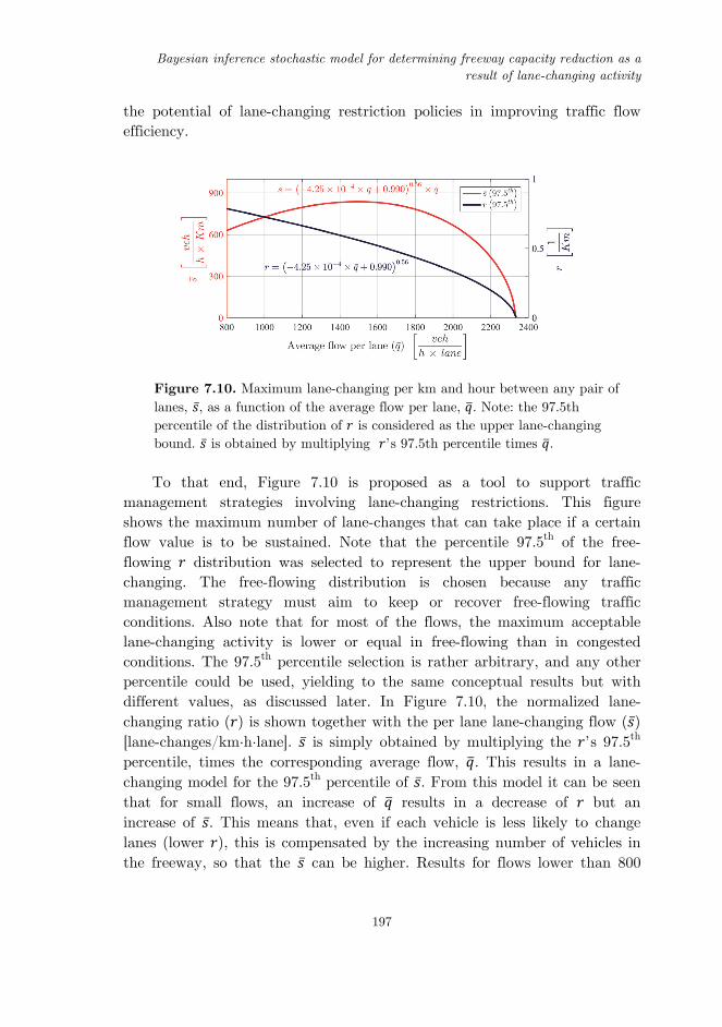
Bayesian inference stochastic model for determining freeway capacity reduction as a result of lane-changing activity

197 

the potential of lane-changing restriction policies in improving traffic flow efficiency.

 

Figure 7.10. Maximum lane-changing per km and hour between any pair of lanes, �̅�, as a function of the average flow per lane, 𝑞. Note: the 97.5th percentile of the distribution of 𝑟 is considered as the upper lane-changing bound. �̅� is obtained by multiplying 𝑟’s 97.5th percentile times 𝑞. To that end, Figure 7.10 is proposed as a tool to support traffic

management strategies involving lane-changing restrictions. This figure shows the maximum number of lane-changes that can take place if a certain flow value is to be sustained. Note that the percentile 97.5th of the free-flowing 𝑟 distribution was selected to represent the upper bound for lane-changing. The free-flowing distribution is chosen because any traffic management strategy must aim to keep or recover free-flowing traffic conditions. Also note that for most of the flows, the maximum acceptable lane-changing activity is lower or equal in free-flowing than in congested conditions. The 97.5th percentile selection is rather arbitrary, and any other percentile could be used, yielding to the same conceptual results but with different values, as discussed later. In Figure 7.10, the normalized lane-changing ratio (𝑟) is shown together with the per lane lane-changing flow (�̅�) [lane-changes/km·h·lane]. �̅� is simply obtained by multiplying the 𝑟’s 97.5th percentile, times the corresponding average flow, 𝑞. This results in a lane-changing model for the 97.5th percentile of �̅�. From this model it can be seen that for small flows, an increase of 𝑞 results in a decrease of 𝑟 but an increase of �̅�. This means that, even if each vehicle is less likely to change lanes (lower 𝑟), this is compensated by the increasing number of vehicles in the freeway, so that the �̅� can be higher. Results for flows lower than 800

Chapter VII 

198 

veh/(h·lane) should be taken with caution and are not represented in Figure 7.10 as few data were collected in this region. Nevertheless, Figure 7.10 is more interesting for flows higher than that of the tipping point (in this case a maximum of �̅� 837 [lane-changes/km·h·lane], corresponding to 𝑟 0.56 [lane-changes/veh·km] when the circulating flow is 1492 [veh/h·lane]) from where the increase of flow does not longer compensate the reduction of 𝑟. In this region, Figure 7.10 can be interpreted as the maximum lane-changing activity that can happen in order to maintain a throughput level. If �̅� (or 𝑟) goes above this threshold, the flow will inevitably decrease.

Given the previous interpretation, the model could be useful for lane-changing control applications, as it determines the maximum acceptable number of lane-changes in order to ensure a desired throughput of the freeway section. Note that the percentile chosen for the upper bound of 𝑟 would represent a tuning parameter of the control algorithm. In the present example, the 97.5th percentile is chosen. This responds to a compromise between the reliability and the severity of the control strategy. Smaller percentiles would increase the reliability in the achievement of the desired flows at the cost of a more restrictive policy, while larger ones would behave in the opposite way: being less reliable but also less restrictive. In fact, the model provides the 𝑟 distribution for any 𝑞. So, in a particular application, any desired probability level could be chosen in the tuning of the control algorithm. This concept is similar to the Sustained Flow Index (SFI) that addresses the trade-off between flow and reliability (Shojaat et al., 2016).

In practice, with the current technology installed in most freeways, everything different from all-or-nothing control (i.e. allow or prohibit) lane-changing might be difficult to implement. In light of this limitation, one strategy could be to prohibit lane-changing when traffic flow reaches a level where small lane-changing ratios could lead to traffic breakdown. Actually, this may be enough in most of the real-world situations, as the objective would be to achieve the maximum possible capacity, 𝑄. An alternative to explore could be the management of vehicles' desired speeds. This control strategy might modify vehicles' speed distribution and consequently impact lane-changing rates. This could be attempted by using dynamic speed limit (DSL) strategies to achieve more uniform travelling speeds and reduce lane-changing rates. In such case, strict enforcement all along the freeway section (e.g. travel time control) would be needed. Otherwise, DSL may lead to the opposite behavior (i.e. increase of lane-changing rates) (Soriguera et al., 2017). In the next future, with the advent of V2I communications, Advanced Driver-Assistance Systems (ADAS) and vehicle automation, lane-changing

Bayesian inference stochastic model for determining freeway capacity reduction as a result of lane-changing activity

199 

control could be feasible by efficiently distributing lane-changing maneuvers amongst vehicles in time and space so that the target lane-changing ratio, 𝑟, could be precisely matched.

5. Conclusions

Lane-changing activity is one of the major disruptors in freeway traffic and a key contributor to traffic instabilities and capacity drop. The research presented in this paper supports this disruptor role of lane-changing in freeways. It has been observed, for multiple locations and days, that lane-changing activity peaks during congestion. Even more, the largest concentration of lane-changes is generally located around shockwaves, at the transition between traffic states. Although no direct evidence has been found confirming that lane-changing activity triggers congestion episodes, a clear relationship between the maximum lane change activity and the maximum average flow per lane has been observed. The lower the maximum lane-changing rate, the larger the maximum flow per lane that can be sustained.

In order to model these qualitative observations, a Bayesian inference stochastic approach is used. This enables to define analytically the relationship between the freeway capacity reduction and the lane-changing activity. Specifically, the normalized lane-changing rate (𝑟) is defined by a heteroscedastic normal distribution with mean and standard deviation decreasing with the average flow per lane (𝑞). This model is useful to determine the maximum lane-changing rate that can be supported in order to ensure a given freeway throughput.

These findings quantify the prevailing theories in the literature arguing that lane-changes are an important traffic disruptor that can trigger congestion. In consequence, largest flows can only be achieved with very low lane-changing rates, as any disruption is enough to breakdown traffic in this highly synchronized flow. Therefore, the theoretical maximum flow (i.e. the capacity) would be achieved in the no lane-changing scenario. For this ideal scenario, the proposed stochastic model is used to derive the probability density function for capacity. The obtained capacity values are somehow larger than the ones empirically observed and proposed in manuals. This confirms the potential of lane-changing control strategies during peak periods in order to improve traffic efficiency. Otherwise, lane-changing can potentially make traffic unstable leading to a capacity reduction (i.e. a

Chapter VII 

200 

capacity drop). Obviously, such control strategies must deal with the existence of mandatory lane-changes near diverging segments.

6. Acknowledgements

Authors acknowledge the collaboration of Mr. Adrià Torres in the counting of lane-changes from video recordings. Also, the comments of Mrs. Margarita Martínez to preliminary versions of the paper have had a positive impact in this final version. The database construction would not have been possible without the collaboration of the Catalan Traffic Administration (Servei Català de Trànsit) and the staff at the Traffic Management Center. The guidance of Prof. Enrique Castillo in the usage of the OpenBUGS software is also gratefully acknowledged. This research has been partially funded by the Spanish Ministry of Economy and Competitiveness (Ministerio de Economía y Competitividad, Gobierno de España), grant number TRA2016-79019-R/COOP.

References

Ahn, S. and Cassidy, M. J. (2007). Freeway traffic oscillations and vehicle lane-change maneuvers. 17th International Symposium Of Transportation and Traffic Theory.

Banks, J. H. (1991). Two-capacity phenomenon at freeway bottlenecks: A basis for ramp metering. Transportation Research Record, 1320, 83–90.

Brilon, W., Geistefeldt, J. and Regler, M. (2005). Reliability of freeway traffic flow: a stochastic concept of capacity. Proceedings of the 16th International Symposium on Transportation and Traffic Theory, 125143.

Cassidy, M. J. and Bertini, R. L. (1999). Some traffic features at freeway bottlenecks. Transportation Research Part B: Methodological, 33(1), 25–42.

Cassidy, M. J., Jang, K. and Daganzo, C. F. (2010). The smoothing effect of carpool lanes on freeway bottlenecks. Transportation Research Part A: Policy and Practice, 44(2), 65–75.

Cassidy, M. J. and Rudjanakanoknad, J. (2005). Increasing the capacity of an isolated merge by metering its on-ramp. Transportation Research Part B: Methodological, 39(10), 896–913.

Bayesian inference stochastic model for determining freeway capacity reduction as a result of lane-changing activity

201 

Cassidy, M. J. and Windover, J. R. (1995). Methodology for assessing dynamics of freeway traffic flow. Transportation Research Record, 1484, 73–79.

Castillo, E., Calviño, A., Grande, Z., Sánchez-Cambronero, S., Gallego, I., Rivas, A. and Menéndez, J. M. (2016a). A Markovian-Bayesian network for risk analysis of high speed and conventional railway lines integrating human errors. Computer-Aided Civil and Infrastructure Engineering, 31(3), 193–218.

Castillo, E., Grande, Z. and Calviño, A. (2016b). Bayesian networks‐based probabilistic safety analysis for railway lines. Computer-Aided Civil and Infrastructure Engineering, 31(9), 681–700.

Castillo, E., Grande, Z., Mora, E., Lo, H. K. and Xu, X. (2017a). Complexity reduction and sensitivity analysis in road probabilistic safety assessment bayesian network models. Computer-Aided Civil and Infrastructure Engineering, 32(7), 546–561.

Castillo, E., Grande, Z., Mora, E., Xu, X. and Lo, H. K. (2017b). Proactive, backward analysis and learning in road probabilistic Bayesian network models. Computer-Aided Civil and Infrastructure Engineering, 32(10), 820–835.

Chen, D., Ahn, S., Laval, J. and Zheng, Z. (2014). On the periodicity of traffic oscillations and capacity drop: the role of driver characteristics. Transportation Research: Part B: Methodological, 59, 117–136.

Chen, D. and Ahn, S. (2018). Capacity-drop at extended bottlenecks: Merge, diverge, and weave. Transportation Research Part B: Methodological, 108, 1-20.

Chung, K., Rudjanakanoknad, J. and Cassidy, M. J. (2007). Relation between traffic density and capacity drop at three freeway bottlenecks. Transportation Research Part B: Methodological, 41(1), 82–95.

Coifman, B. and Li, L. (2017). A critical evaluation of the Next Generation Simulation (NGSIM) vehicle trajectory dataset. Transportation Research Part B: Methodological, 105, 362–377.

Coifman, B., Mishalani, R., Wang, C., Krishnamurthy, S. and Harris, A. D. (2006). Impact of lane-change maneuvers on congested freeway segment delays: Pilot study. Transportation Research Record, 1965, 152–159.

Deublein, M., Matthias, S., Adey, B. T. and García de Soto, B. (2015). A Bayesian network model to predict accidents on Swiss highways. Infrastructure Asset Management, 2(4), 145–158.

Chapter VII 

202 

Elefteriadou, L., Roess, R. P. and McShane, W. R. (1995). Probabilistic nature of breakdown at freeway merge junctions. Transportation Research Record, 1484, 80–89.

Elefteriadou, L., Roess, R.P. and McShane, W.R. (2005). Probabilistic nature of breakdown at freeway merge junctions. Transportation Research Record, 1484, 80–89.

Engle, R. F. (1982). Autoregressive conditional heteroscedasticity with estimates of the variance of United Kingdom inflation. Econometrica, 50(4), 987–1007.

Federal Highway Administration. (2006). Interstate 80 Freeway Dataset Factsheet. Fhwa-Hrt-06-137. Retrieved from: http://www.fhwa.dot.gov/publications/research/operations/06137/

Federal Highway Administration. (2015). Next Generation Simulation (NGSIM). Retrieved March 3, 2016, from:

http://ops.fhwa.dot.gov/trafficanalysistools/ngsim.htm.

François, O. and Laval, G. (2011). Deviance information criteria for model selection in approximate Bayesian computation. Statistical Applications in Genetics and Molecular Biology, 10(1), 1-25.

Gilks, W. R., Richardson, S. and Spiegelhalter, D. J. (1996). Markov Chain Monte Carlo in practice. London: Chapman and Hall.

Gelfand A.E. and Smith A.F.M. (1990). Sampling-based approaches to calculating marginal densities. Journal of the American Statistical Association, 85, 398–409.

Geistefeldt, J. and Brilon, W. (2009). A comparative assessment of stochastic capacity estimation methods. In: Lam W., Wong S., Lo H. (eds) Transportation and Traffic Theory 2009: Golden Jubilee. Springer, Boston, MA.

Gelman, A., Carlin, J. B., Stern, H. S., Dunson, D. B., Vehtari, A. and Rubin, D. B. (2014). Bayesian data analysis. CRC Texts in Statistical Science. Chapman & Hall.

Goñi-Ros, B., Knoop, V.L., Takahashi, T., Sakata, I., van Arem, B., Hoogendoorn, S.P. (2016). Optimization of traffic flow at freeway sags by controlling the acceleration of vehicles equipped with in-car systems. Transportation Research: Part C: Emerging Technologies, 71, 1–18.

Bayesian inference stochastic model for determining freeway capacity reduction as a result of lane-changing activity

203 

Hall, F. L. and Agyemang-Duah, K. (1991). Freeway capacity drop and the definition of capacity. Transportation Research Record, 1320, 91–98.

Hashemi, H. and Abdelghany, K. (2018). End‐to‐end deep learning methodology for real‐time traffic network management. Computer‐Aided Civil and Infrastructure Engineering, 33(10), 849-863.

Hatakenaka, H., Hirasawa, T., Yamada, K., Yamada, H., Katayama, Y. and Maeda, M. (2004). Development of AHS for Traffic Congestion in SAG Sections. 13th World Congress on ITS.

Highway Capacity Manual. (2010). Transportation Research Board, National Research Council, Washington, DC.

Hossain, M. and Muromachi, Y. (2012). A Bayesian network based framework for real-time crash prediction on the basic freeway segments of urban expressways. Accident Analysis & Prevention, 45, 373–381.

Huang, Y. and Beck, J. L. (2018). Full Gibbs sampling procedure for Bayesian system identification incorporating sparse Bayesian learning with automatic relevance determination. Computer‐Aided Civil and Infrastructure Engineering.

Ibrahim, A. T. and Hall, F. L. (1994). Effect of adverse weather conditions on speed-flow occupancy relationships. Transportation Research Record, 1457, 184–191.

Jia, A., Zhou, X., Li, M., Rouphail, N. M. and Williams, B. M. (2011). Incorporating stochastic road capacity into day-to-day traffic simulation and traveler learning framework: Model development and case study. Transportation Research Record, 2254(1), 112–121.

Jin, W. L. (2010). A kinematic wave theory of lane-changing traffic flow. Transportation Research Part B: Methodological, 44(8-9), 1001–1021.

Jin, C. J., Knoop, V. L., Li, D., Meng, L. Y. and Wang, H. (2019). Discretionary lane-changing behavior: empirical validation for one realistic rule-based model. Transportmetrica A: Transport Science, 15(2), 244-262.

Knoop, V. , Hoogendoorn, S. , Adams, K. (2009). Capacity reductions at incidents sites on motorways. European Journal of Transportation and Infrastructures Research, 9, 363–379.

Lamm, R., Choueiri, E. M. and Mailaender, T. (1987). Comparison of operating speed on dry and wet pavement of two lane rural highways. Transportation Research Record, 1280, 199–207.

Chapter VII 

204 

Laval, J. A. and Daganzo, C. F. (2006). Lane-changing in traffic streams. Transportation Research Part B: Methodological, 40(3), 251–264.

Leclercq, L., Laval, J. A. and Chiabaut, N. (2011). Capacity drops at merges: An endogenous model. Procedia-Social and Behavioral Sciences, 17, 12-26.

Liu, Q., Wang, B. and Zhu, Y. (2018). Short‐term traffic speed forecasting based on attention convolutional neural network for arterials. Computer‐Aided Civil and Infrastructure Engineering, 33(11), 999-1016.

Lorenz, M. and Elefteriadou, L. (2000). A probabilistic approach to defining freeway capacity and breakdown. TRB-Circular E-C018, Transportation Research Board, 84–95.

Lunn, D., Spiegelhalter, D., Thomas, A. and Best, N. (2009). The BUGS project: Evolution, critique and future directions. Statistics in Medicine, 28, 3049-3067.

Lv. Y., Duan, Y., Kang, W. and Wang, F. Y. (2015). Traffic flow prediction with big data : A deep learning approach. IEEE Trans. Intelligent Transportation Systems, 16(2), 865-873.

Marczak, F., Daamen, W. and Buisson, C. (2014). Empirical analysis of lane changing behaviour at a freeway weaving section. Transport Research Arena (TRA) 5th Conference: Transport Solutions from Research to Deployment, Institut Francais des Sciences et Technologies des Transports, de l’Aménagement et des Réseaux. IFSTTAR.

Marczak, F., Leclercq, L. and Buisson, C. (2015). A Macroscopic model for freeway weaving sections. Computer‐Aided Civil and Infrastructure Engineering, 30(6), 464-477.

Mauch, M. and Cassidy, M. J. (2002). Freeway traffic oscillations: observations and predictions. Transportation and Traffic Theory in the 21st Century: Proceedings of the 15th International Symposium on Transportation and Traffic Theory, Adelaide, Australia, 16-18 July 2002, 653-673.

Menendez, M. and Daganzo, C. F. (2007). Effects of HOV lanes on freeway bottlenecks. Transportation Research Part B: Methodological, 41(8), 809–822.

Mihaylova, L., Boel, R. and Hegyi, A. (2007). Freeway traffic estimation within particle filtering framework. Automatica, 43(2), 290–300.

Minderhoud, M. M., Botma, H. B. and Bovy, P. H. L. (1997). Assessment of roadway capacity estimation methods. Transportation Research Record, 1572, 59–67.

Bayesian inference stochastic model for determining freeway capacity reduction as a result of lane-changing activity

205 

Montanino, M. and Punzo, V. (2015). Trajectory data reconstruction and simulation-based validation against macroscopic traffic patterns. Transportation Research Part B: Methodological, 80, 82–106.

Muñoz, J.C. and Daganzo, C.F. (2002). The bottleneck mechanism of a freeway diverge. Transportation Research Part A: Policy and Practice, 36(6), 483–505.

Oh, S. and Yeo, H. (2012). Estimation of capacity drop in highway merging sections. Transportation Research Record, 2286(1), 111–121.

Oh, S. and Yeo, H. (2015). Impact of stop-and-go waves and lane changes on discharge rate in recovery flow. Transportation Research: Part B Methodological, 77, 88–102.

Okamura, H., Watanabe, S. and Watanabe, T. (2000). An empirical study on the capacity of bottlenecks on the basic suburban expressway sections in Japan. Proceedings of the 4th International Symposium on Highway Capacity,12, 120-129.

de Oña, J., Mujalli, R. O. and Calvo, F. J. (2011). Analysis of traffic accident injury severity on Spanish rural highways using Bayesian networks. Accident Analysis and Prevention, 43(1), 402–411.

Ozbay, K. and Ozguven, E. E. (2007). A comparative methodology for estimating the capacity of a freeway section. IEEE Intelligent Transportation Systems Conference, 1034-1039. Seattle, WA.

Patire, A. D. and Cassidy, M. J. (2011). Lane changing patterns of bane and benefit: Observations of an uphill expressway. Transportation Research Part B: Methodological, 45(4), 656–666.

Persaud, B., Yagar, S. and Brownlee, R. (1998). Exploration of the breakdown phenomenon in freeway traffic. Transportation Research Record, 1634, 64–69.

Polus, A. and Pollatschek, M. A. (2001). Stochastic nature of freeway capacity and its estimation. Canadian Journal of Civil Engineering, 29(6), 842-852.

Punzo, V., Borzacchiello, M. T. and Ciuffo, B. (2011). On the assessment of vehicle trajectory data accuracy and application to the Next Generation SIMulation (NGSIM) program data. Transportation Research Part C: Emerging Technologies, 19(6), 1243–1262.

Sala, M., Soriguera, F., Huillca, K. and Vilaplana, V. (2019). Measuring traffic lane‐changing by converting video into space–time still images. Computer‐Aided Civil and Infrastructure Engineering, 34(6), 488-505.

Chapter VII 

206 

Shojaat, S., Geistefeldt, J., Parr, S. A., Wilmot, C. G. and Wolshon, B. (2016). Sustained flow index: Stochastic measure of freeway performance. Transportation Research Record, 2554, 158-165.

Smith, B. L., Byrne, K. G., Copperman, R. B., Hennessy, S. M. and Goodall, N. J. (2004). An investigation into the impact of rainfall on freeway traffic flow. In 83rd Annual Meeting of the Transportation Research Board, Washington DC.

Soriguera, F., Martínez, I., Sala, M. and Menéndez, M. (2017). Effects of low speed limits on freeway traffic flow. Transportation Research Part C: Emerging Technologies, 77, 257–274.

Soriguera, F. and Sala, M. (2014). Experimenting with dynamic speed limits on freeways. Procedia Social and Behavioral Sciences, 160, 35–44.

Spiegelhalter D. J., Best, N. G., Carlin, B. P. and van der Linde, A. (2002) Bayesian measures of model complexity and fit (with discussion). Journal of the Royal Statistical Society Series B, 64(4), 583–639.

Srivastava, A. and Geroliminis, N. (2013). Empirical observations of capacity drop in freeway merges with ramp control and integration in a first-order model. Transportation Research Part C: Emerging Technologies, 30, 161–177.

Sun, D. J. and Elefteriadou, L. (2012). Lane-changing behavior on urban streets: An “in-vehicle” field experiment-based study. Computer-Aided Civil and Infrastructure Engineering, 27(7), 525–542.

Sun, D. J. and Kondyli, A. (2010). Modeling vehicle interactions during lane-changing behavior on arterial streets. Computer-Aided Civil and Infrastructure Engineering, 25(8), 557–571.

Sun, S., Zhang, C. and Yu, G. (2006). A Bayesian network approach to traffic flow forecasting. IEEE Transactions on Intelligent Transportation Systems, 7(1), 124–133.

Tajalli, M. and Hajbabaie, A. (2018). Dynamic speed harmonization in connected urban street networks. Computer‐Aided Civil and Infrastructure Engineering, 33(6), 510-523.

Vrontos, I. D., Dellaportas, P. and Politis, D. N. (2000). Full Bayesian inference for GARCH and EGARCH models. Journal of Business & Economic Statistics, 18(2), 187-198.

Bayesian inference stochastic model for determining freeway capacity reduction as a result of lane-changing activity

207 

Wang, C. and Coifman, B. (2008). The effect of lane-change maneuvers on a simplified car-following theory. IEEE Transactions on Intelligent Transportation Systems, 9(3), 523–535.

Yao, B., Chen, C., Cao, Q., Jin, L., Zhang, M., Zhu, H. and Yu, B. (2017). Short‐term traffic speed prediction for an urban corridor. Computer‐Aided Civil and Infrastructure Engineering, 32(2), 154-169.

Yeon, J., Hernandez, S. and Elefteriadou, L. (2009). Differences in freeway capacity by day of the week, time of day, and segment type. Journal of Transportation Engineering, 135(7), 416–426.

Yildirim, I. (2012). Bayesian inference: Gibbs sampling. Technical Note, University of Rochester.

Yin, H., Wong, S., Xu, J. and Wong, C. K. (2002). Urban traffic flow prediction using a fuzzy-neural approach. Transportation Research Part C: Emerging Technologies, 10(2), 85–98.

Yuan, K., Laval, J., Knoop, V. L., Jiang, R. and Hoogendoorn, S. P. (2019). A geometric Brownian motion car-following model: towards a better understanding of capacity drop, Transportmetrica B: Transport Dynamics, 7:1, 915-927.

Yuan, K., Knoop, V. L. and Hoogendoorn, S. P. (2015). Capacity drop relationship between speed in congestion and the queue discharge rate. Transportation Research Record, 2491, 72–80.

Chapter VIII

Macroscopic Modeling of Connected Autonomous Vehicles Platoons under Mixed Traffic Conditions

Submitted in Transportation Research Procedia.

Macroscopic Modeling of Connected Autonomous Vehicles Platoons under Mixed Traffic Conditions

211 

Macroscopic Modeling of Connected Autonomous Vehicles Platoons under Mixed

Traffic Conditions

Marcel Sala*a and Francesc Sorigueraa

aBarcelona Innovative Transport – UPC – Barcelona Tech, Jordi Girona 1-3,

Building B1, Office 114, 08034 Barcelona, Spain. Abstract Autonomous vehicles (AV) will be present in freeways, and they will have to share current infrastructure with human driven vehicles. This mixed traffic scenario needs to be planed and managed. Some research points that an AV mismanagement could lead to a capacity decrease. This can be solved with connected AV traveling in platoons. Some research exist to that end, but all of them is done using microsimulation tools. These are very powerful and detailed tools but have the shortcoming of strongly rely on an uncertain calibration and give limited insights to the problem. The more robust and simpler to understand macroscopic tools, have almost no platooning models yet. The research presented in this paper fills the gap, by providing a generalized macroscopic model to estimate the average length in vehicle for platoons. This is done by giving a set of rules for AV to form a platoon, including two different platooning schemes representing the best and worst case scenarios. This is of a key importance as greater platoon length is the main factor to drive capacity improvements on highways, which under the appropriate conditions can exceed 10.000 vehicles per hour and lane. Keywords: platoon; cooperative traffic, autonomous vehicles, connected vehicles, highway capacity, macroscopic model.

* Corresponding author

Chapter VIII 

212 

1. Introduction and background

In recent years technology has been evolving at a remarkable pace. In the field of road transportation. This is mainly observed as: introduction of newer and more advanced driver assist systems and the development of new and more efficient powertrains. While the latter is expected to have a great impact in terms of energy consumption and pollution is only the former factor the one having the potential to change the vehicles behavior to tackle congestion and safety problems.

While some of the early electronic drivers’ assist systems had the only purpose to improve safety, such as the Anti Block System (ABS) or the Electronic Stability Control (ESC or ESP). Modern ones aim to partially automate driving as for instance is the ACC (Adaptive Cruise Control) or lane keeping technologies, being the final goal to achieve full automation in the form of Autonomous Vehicles (AV). There is some debate on how long it will take for AVs to be reality outside of pilot tests. But exists some consensus that will eventually happen after solving the great technological challenges AV present (Martinez et al., 2018).

Nonetheless, the aim of this paper is not to discuss the technological challenges, but to set the path of a macroscopic model for platoons of Cooperative Autonomous Vehicles (CAV) at highways. This is important as early studies on partial automation system showed, that congestion, not only will not be solved by AVs but can even be worsened. For instance, greater time gaps and lower acceleration typically in Adaptative Cruise Control (ACC) systems greatly reduce the capacity (Ntousakisa et al. 2014). Thus, in order to increase the capacity the average headway needs to decrease (Taieb-Maimo, and Shinar, 2001; Lin et al., 2009; Shladover et al., 2012; Lioris et al., 2017). Exist different ways of achieving it, as current ACC have reaction time ranging between 0.1 and 0.2 seconds (Ketsing at al. 2007). Thus, the problem is users selecting these possible shorter gaps and still feel safe (Taieb-Maimo, and Shinar, 2001; Rahman et al., 2017, Lin et al., 2009). However, CACC (Coperative ACC) is generally preferred, as it has the potential to achieve even shorter gaps while being still safe. In particular, platooning which is a string of consecutive CACC vehicles traveling at a very short time gaps. This will not only have the possibility to increase capacity, but it also reduces the energy consumption of the vehicles traveling at short gaps (Alam et al., 2010; Tsugawa et al., 2011; Shida et al., 2010).

Macroscopic Modeling of Connected Autonomous Vehicles Platoons under Mixed Traffic Conditions

213 

However, to achieve significant capacity improvements is necessary to have long platoons; as the first vehicle in the platoon will not travel at a reduced headway. Thus, knowing which traffic conditions could potentially result in longer platoons, which would imply greater capacity is of a key importance. The advantage of using macroscopic models is that they rely in simpler models which in turn require fewer inputs. This allows to a better understanding of the phenomena trade-off, at the cost of losing some level of detail. To the authors best knowledge exists just one initial approach to macroscopically model CAV platoons (Chen at al., 2017). This contribution is of great interest, as it quantifies the impact of different parameters and policies on the road capacity. However, it avoids tackling any traffic dynamics nor how different traffic conditions can affect the platoon length. This is precisely the gap this paper fills by providing traffic related platoons, using two different platoon schemes which aim to be representative of the reality. Also, estimates on the capacity for the given methodology are provided. The paper is structured as follows: in section 2 the problem and variables definitions are made. Following, in section 3 the model is presented along with some results on the average platoon length estimation. In section 4 estimates of capacity for different platoon models and penetration rates are presented and finally at section 5 some conclusions are outlined.

2. Definitions

 

Figure 8.1: Platoon components illustration. The model considers a highway with mixed traffic, which means CAVs

and RV (Regular Vehicles) sharing the infrastructure. Platoons are consecutive strings of CAVs traveling at a shorter gaps than RVs. Note that by definition any RV splits one platoon into two different ones. Vehicles in a platoon are classified as: i) platoon leader, which is the first vehicle of the string and ii) platoon follower, which is any vehicle in the platoon behind the leader, see Figure 8.1 for further clarifications. For sake of briefness, they will be referred as leader and followers. Note that only followers travel at reduced

Chapter VIII 

214 

gaps, since leaders have no cooperative information of the vehicle in front. A single CAV is considered to be itself a platoon, which their only component is the leader. The model inputs are defined in Table 8.1. The endogenous computational variables are defined in Table 8.2.

Table 8.1. Input definitions.

Table 8.2. Variable definitions.

3. Platoon length estimation

In order to estimate the platoon length is necessary to make some assumptions on how platoons will actually take place, i.e. the formation dynamics. In this paper is assumed that: i) the process to join a platoon is instantaneous (no time); ii) vehicles only consider to join a platoon or merge with other CAVs within the platoon range (l ). The first assumption is reasonable as long as the time it takes for one vehicle to join a platoon is negligible in comparison with the time then it travels within the platoon. This time depends on many different factors as: speed differential, l , etc. The second one is placed as there will be some communication range limit. Literature points out that currently 5.9-GHz DSRC communication

Input Units Description 𝑞 [veh/h] Total demand. 𝑧 [# lanes] Total number of lanes. 𝑣 [Km/h] Lane speed. 𝛽 [pu] Penetration rate of the CAV over the total demand. 𝑙 [Km] Platooning range. 𝐿 [veh/platoon] Maximum allowed platoon length in vehicles.

Variable Units Description

𝑎 , [veh] Platoon length. Subindex 𝑖 can be 𝑐 for cooperative or 𝑜 for opportunistic. Subindex 𝑗 stands for the max platoon length 𝐿

𝑚 [platoons] Number of platoons. 𝑠 [platoons] Number of times a platoon has to be split to fulfill 𝐿 . 𝜆 [veh] Average number of vehicles per lane in the 𝑙 distance. 𝑛 [veh] Deterministic sample size.

𝑝 𝜆; 𝑛 [pu] Zero Truncated Poison Distribution probability for 𝑛 with a Poisson parameter 𝜆.

Macroscopic Modeling of Connected Autonomous Vehicles Platoons under Mixed Traffic Conditions

215 

technology provides at least 300 m of communication range (Shladover et al., 2015).

Still, different platoon schemes under the previous hypothesis can be considered. In this paper two possibilities are taken into account and presented: cooperative and opportunistic platooning. Under the cooperative scheme, any CAV within the platoon range will join a single platoon. While on the opportunistic platoon only already consecutive CAVs will form a platoon. This means that platoon length is limited to those CAVs that by chance are already consecutive, and any RV will cut the platoon. It could be argued on how these two schemes are realistic or not, but this will mainly depend on how platooning formation is implemented in a future. Nonetheless, the two presented options, aim to be representative of the best case scenario (cooperative) giving the longest possible platoons at the cost of a much more complex formation, and the worse case scenario (opportunistic), giving the shortest possible platoon, as nothing is done to enlarge them. Of course, shorter than opportunistic platoons are feasible, but to achieve that, some strategy to actively shorten the platoon length would be required. And the only strategy that falls in this category that seems reasonable to be ever implemented, is to enforce a maximum platoon length (L ), which will be considered further on in this section. Indeed some research points out that a maximum platoon length needs to be enforced, since long platoons could exhibit string instabilities. Shladover et al., (2015) states that a maximum platoon length of 20 vehicles can be considered, and in order to achieve this length, a careful platoon design is required.

The average platoon length will depend on how many vehicles are in a given region. The vehicle distribution is assumed to follow a Poisson distribution (Daganzo, 1997). However, only regions with at least one vehicle are of interest. As the ones with no vehicles, have no impact to the platoon mean length. This is represented by a ZTPD (Zero Truncated Poisson Distribution). The probability mass function of the ZTPD p is given in equation (8.1). The formula to compute the Poison parameter λ is given at equation (8.2). Note that λ represents the average number of vehicles both CAVs and RVs) within the platoon range l , and n the actual number of vehicles.

𝑝 𝑁 𝑛; 𝜆𝑒 𝜆

𝑛! 1 𝑒 ; 𝑛 ∈ ℕ∗ (8.1)

Chapter VIII 

216 

𝜆𝑞𝑧

𝑙𝑣

(8.2)

3.1. Cooperative average platoon length

When following the cooperative scheme and no platoon length limits is imposed, all CAVs within the platooning region will form platoon a single platoon. Thus, the average platoon length is just the average number of CAVs in this region. Since the amount of CAVs is a fraction β of the total number of vehicles λ, the average platoon length is shown at equation (8.3) as the ZTPD mean with a parameter λ β. When a maximum platoon length is enforced, whenever than more than L CAVs are in range, these will have to be split into multiple platoons. The minimum number of platoons to be split s is shown in equation (8.4), where ⌈ ⌉ represents the nearest upper integer. Of course, this is 1 when there is no limit. Thus, the average platoon length now is computed as in equation (8.5).

𝑎 ,𝜆 𝛽

1 𝑒 (8.3)

𝑠 𝑎

𝐿; 𝐿 ∞

1 ; 𝐿 ∞ (8.4)

𝑎 ,∑ 𝑝 𝜆 𝛽, 𝑘 𝑎∑ 𝑝 𝜆 𝛽, 𝑘 𝑠

(8.5)

3.2. Opportunistic platooning

The conceptual problem to solve in this section can be conceptualized as: determine the average number of consecutive successes in a Bernoulli experiment with a constant success probability β in a sample of arbitrary size n. A success is considered to be a CAV while a failure represents a RV. Each vehicle in the sample is considered to have an independent probability of being a CAV, and this is equal to β. Thus, each vehicle can be seen as a Bernoulli experiment with a success probability β. This apparently simple problem involves some complexity. Think of a single platoon of length k, it has a probability to happen as described in equation (8.6). Note that when

Macroscopic Modeling of Connected Autonomous Vehicles Platoons under Mixed Traffic Conditions

217 

the platoon length is smaller than the sample, a failure is required to “cut” the success string (i.e. the platoon). However, this is for a single platoon, and when a 1 n, other platoons can also happen simultaneously in the same sample. For any n exists a finite (could be very large) number of combinations on which the successes and failures (CAVs and RVs) can be sorted. This problem is solved at Theorem 2.1 form Makri and Psillakis (2011), shown at equation (8.7), which gives the probability of having exactly m platoons of exactly a vehicles long in a sample of size n, given an independent success probability β. The binomial coefficients are the extended ones as defined in equation (8.8), with no support for negative numbers.

𝛽 , 𝑛 𝑎

𝛽 1 𝛽 , 𝑎 𝑘 (8.6)

𝑃 𝐸 , 𝑚 𝛽 1 𝛽 𝑦 1𝑚

1𝑦 1 𝑚

𝑗

𝑛 𝑎 1 𝑚 𝑗𝑛 𝑦 𝑎 𝑚 𝑗

;

𝑎 ∈ 1, 𝑛 ; 𝑚 ∈ 1,𝑛 1𝑎 1

(8.7)

𝑐𝑑

𝑐 𝑐 1 𝑐 𝑑 1

𝑑!; 𝑑 ∈ ℕ0, 𝑐 ∈ ℝ , 𝑐 𝑑 (8.8)

Since the binomial coefficient is involved, the problem becomes

numerically unstable (overflow) for large samples. A solution to this is provided in Remark 2.3 of Makri and Psillakis (2011) as a normal approximation when n ≫ 1, see equation (8.10), with Φ meaning normal N 0,1 cumulative distribution function. In the current paper this is used for n 100. Values for μ and σ are defined in equation (8.9). Note that this approximation can only be used when the conditions at equation (8.11) are met.

Chapter VIII 

218 

𝜇 1 𝛽 𝛽

𝜎 𝜇 1 𝜇 21 𝛽

𝛽𝑎 1

(8.9)

𝑃 𝐸 , 𝑚 Φ𝑚 0.5 𝑛 ∗ 𝜇

𝜎 √𝑛Φ

𝑚 0.5 𝑛 ∗ 𝜇

𝜎 √𝑛 (8.10)

𝜇3 𝜎

√𝑛0 𝑎𝑛𝑑 𝜇

3 𝜎

√𝑛

𝑛 1𝑎 1

𝑛 (8.11)

So far, only the probabilities of having exactly m platoons of length a in

a sample n are known, the mean is still unknown. The definition of the mean implies adding all the probabilities multiplied by the variable value. However to do so, the sum of the probabilities need to add 1, and this is not the case. Still the probabilities are correct, the reason of that is that some combinations can happen at the same time that others happen too. For instance in a sample of size 20, two platoons of 3 vehicles do not exclude that one platoon of 5 vehicles could happen too. Adding all the combinations as shown in equation (8.12) results not on the average platoon length but on the average total number of CAVs in the sample n, which is n β. Equations (8.7) and (8.10) can be used to compute the mean number of platoons in the sample (m) as shown in equation (8.13). Dividing the average total number of CAVs by the average number of platons in the sample gives the average platoon length (a) in the sample of size n, see equation (8.14). The average platoon length in a region with an average number of vehicles equal to λ, on which the vehicles follow a Poisson distribution is given at equation (8.15). Similar results can be obtained preforming a Montecarlo simulation enough times.

𝑛 𝛽 𝑎𝑠

𝑚 𝑠 𝑃 𝐸 , 𝑚 (8.12)

𝑚 𝑛, 𝛽 𝑚 𝑠 𝑃 𝐸 , 𝑚 (8.13)

Macroscopic Modeling of Connected Autonomous Vehicles Platoons under Mixed Traffic Conditions

219 

𝑎 𝑛, 𝛽𝑛 𝛽

𝑚 𝑛, 𝛽 (8.14)

𝑎 , 𝜆, 𝛽 𝑝 𝜆, 𝑛 𝑎 𝑛, 𝛽 (8.15)

3.3. Comparing platoon schemes.

In Figure 8.2, the average platoon length for both types of platoon is presented for an average number of vehicles within the platooning range up to λ 100. Both types of platoons are presented for no maximum platoon length L ∞ and for a maximum platoon length of 20 vehicles L20 . Additional comparison plots are presented at Figure 8.3.

Figure 8.2: Average platoon lengths under different demands, AV penetration rates and platooning schemes.

(a) (b)

(c) (d)

Chapter VIII 

220 

Figure 8.2 (a) shows the cooperative platoon with no length limit. This is the same as showing the ZTPD mean presented in equation (8.3), which is the average amount of CAVs. However, when a maximum platoon is imposed, the results change, see Figure 8.2 (c). Apart from all values being equal or smaller than 20, a much shorter average platoon length can be observed in the region nearby λ β 20, this is because any platoon that exceeds 20 vehicles is split into two platoons, effectively shortening the average length. When observing the results of opportunistic platoon, Figure 8.2 (b) and (d), is evident that the average length is much more sensible to the value of β than it is to λ. The latter has only impact when demand is small enough, so the average length of the platoon is limited due to the lack of CAVs to form a long enough platoon. As the penetration rate increases (β), it also increases the likelihood of having longer platoons. Thus, is when 𝛽 is close to one that average platoon length shows sensitivity to both penetration rate and average number of vehicles.

Figure 8.3 shows the comparison between the two purposed platooning strategies as the subtraction of average platoon length, for no platoon length limit (Figure 8.3a) and a platoon limit of 20 vehicles (Figure 8.3b). In both Figure 8.3a and 8.3b, when β is either zero or one, there is no difference between platooning schemes. The explanation is simple, as for β 0, there are no CAVs, thus no platoons and both have the same average length of one vehicle. For β 1 there are no RV, and since the only thing that makes opportunistic platooning shorter than cooperative are RV cutting the otherwise longer platoons, the platoon length is the same no matter the scheme. The greatest difference between schemes is for mid range penetration rates with big demands. Is in this zone where there is plenty of CAV to form long platoons but also of RVs to cut them if nothing is made to avoid it. The comparison between Figure 8.3 (a) and (b), shows that differences between platooning schemes are much smaller when a maximum platoon length is enforced. This is, as the cooperative platooning produces much shorter platoons when a maximum length is enforced, see Figure 8.2 (a) and (c).

Macroscopic Modeling of Connected Autonomous Vehicles Platoons under Mixed Traffic Conditions

221 

Figure 8.3: Comparaison between cooperative and opportunistic platooning in terms of average platoon length. a) No platoon length limit. b) Maximum length of 20 vehicles platoon.

4. Mixed lane capacity

In this section, an idea of the capacities that could be achieved using the platoon schemes presented is given. To do so, is necessary to assume some values regarding the vehicles. These are: a speed of 120 Km/h, a vehicular length of 5 meters and a time gap of 1.5 seconds for RV and platoon leaders, and of 0.1 seconds for platoon followers. With these values, is possible to compute the mean headway given the CAV penetration rate. This is done for both platoon schemes and for no platoon limit and a limit of 20 vehicles per platoon. Thus, the lane capacities per each of the four possible combinations through the whole range of CAV penetration is obtained and shown at

(a)

(b)

Chapter VIII 

222 

Figure 8.4. The capacities that can be achieved are huge. As for instance with a 100% of CAV in any of the possible combinations, the lane capacity exceeds 10.000 veh/h/lane. This is more than 4 times the value with no CAVs at all, which is 2308 veh/h/lane. Capacity values for a 50% penetration rate, are 3407 veh/h/lane under cooperative platooning and 2811 veh/h/lane for opportunistic. Another interesting question that can be observed form Figure 8.4, is that enforcing a platoon limit, in terms of capacity only has a meaningful effect for great penetration rates, in excess of 90% of CAVs. In lower penetration rates, the differences are indistinguishable.

Figure 8.4: CAV penetration rate vs lane capacity for both platooning schemes (cooperative and opportunistic) and maximum platoon length of ∞ and 20 vehicles per platoon.

5. Conclusions

The presented methodology to estimate platoon length is a key step in order to achieve a macroscopic model that can model traffic dynamics with platoons. As is crucial to be able to model how the different traffic states produce different platoons. Since only platoon followers travel at a reduced gap (or time gap), they are the only vehicles to actually contribute towards increasing the lane capacity. Thus, the longer the platoons, the more followers in them and greater lane capacities can be achieved. Of course not only traffic will affect the platoon length, but also how they form. To that end two methodologies were presented, which aim to represent the best case scenario (cooperative) and the worst case scenario (opportunistic) in terms of platoon length. The specific dynamics of platoon formation have been neglected to achieve a simple but understandable model.

Macroscopic Modeling of Connected Autonomous Vehicles Platoons under Mixed Traffic Conditions

223 

Additionally, the possibility to enforce a maximum platoon length is presented. This could be of interest due to technological limits on how long the platoon could be or enforced by a traffic administration. Enforcing a maximum of 20 vehicles per platoon has the strongest effect on the cooperative platoon (see Figure 8.2 a and c). Still when this is translated to lane capacities, the differences are only noticeable for both types of platoon at penetration rates that exceed 90% of CAVs. And speaking of capacity, here the main conclusions can be obtained. In any case the capacity is increased, being more noticeable the grater the penetration rate is, for a 50% penetration rate the increase is 22% for opportunistic and 48% for cooperative. Under the best possible conditions it achieves values in excess of 12000 veh/h/lane, which is 5,3 times the values achieved for RV with the same parameters.

6. Acknowledgements

Authors want to acknowledge Frosso Makri that has shared some knowledge on how to compute the average opportunistic platoon mean. Also Marcos Medina and Enrique Jimenez are acknowledged for some useful comments on how to better explain and show some of the results presented in this reasearch. This research has been partially funded by the Spanish Ministry of Economy and Competitiveness (Ministerio de Economía y Competitividad, Gobierno de España), grant number TRA2016-79019-R/COOP.

References

Alam, A.A., Gattami, A. and Johansson, K. H. (2010). An Experimental Study on the Fuel Reduction Potential of Heavy Duty Vehicle Platooning. Proceedings, 13th International IEEE Annual Conference on Intelligent Transportation Systems, Madeira Island, Portugal.

Chen, D., Ahn, S., Chitturi, M. and Noyce, D. A. (2017). Towards vehicle automation: Roadway capacity formulation for traffic mixed with regular and automated vehicles. Transportation research part B: methodological, 100, 196-221.

Daganzo, C. F. (1997). Fundamentals of transportation and traffic operations (Vol. 30). Oxford: Pergamon.

Chapter VIII 

224 

Kesting, A., Treiber, M., Schönhof, M. and Helbing, D. (2007). Extending Adaptive Cruise Control to Adaptive Driving Strategies. Transportaion Research Record 2000, 16–24.

Lin, T., Hwang, S. and Green, P.A. (2009). Effects of time-gap settings of adaptive cruise control (ACC) on driving performance and subjective acceptance in a bus driving simulator. Safety Science 47, 620–625.

Lioris, J., Pedarsani, R., Tascikaraoglu, F. Y., aand Varaiya, P. (2017). Platoons of connected vehicles can double throughput in urban roads. Transportation Research Part C: Emerging Technologies, 77, 292-305.

Makri, F. S. and Psillakis, Z. M. (2011). On success runs of a fixed length in Bernoulli sequences: Exact and asymptotic results. Computers & Mathematics with Applications, 61(4), 761-772.

Martínez, M., Soriguera, F. and Pérez, I. (2018). Autonomous driving: a bird's eye view. IET intelligent transport systems, 1-17.

Ntousakisa, I. A., Nikolosa, I. K., and Papageorgiou, M. (2014). On Microscopic Modelling of Adaptive Cruise Control Systems. 4th International Symposium of Transport Simulation-ISTS’14, 1-4 June 2014, Corsica, France.

Rahman, M., Chowdhury, M., Dey, K., Islam, R., and Khan, T. (2017). An Evaluation Strategy for Driver Car Following Behavior Models for CACC Controllers. Transportation Research Record 2622, 84-95

Shida, M., Doi, T., Nemoto, Y. and Tadakuma, K. (2010). A Short-Distance Vehicle Platooning System, 2nd Report: Evaluation of Fuel Savings by the Developed Cooperative Control. Proceedings, 10th International Symposium on Advanced Vehicle Control (AVEC), Loughborough, United Kingdom, KTH Royal Institute of Technology, Stockholm, Sweden, 719–723.

Shladover, S.E., Su, D. and Lu X.Y. (2012), Impacts of cooperative adaptive cruise control on freeway traffic flow. Transportation Research Record 2324, 63-70.

Shladover, S. E., Nowakowski, C., Lu, X. Y., and Ferlis, R. (2015). Cooperative adaptive cruise control: Definitions and operating concepts. Transportation Research Record, 2489, 145-152.

Taieb-Maimon, M., and Shinar D. (2001). Minimum and comfortable driving headways: Realityversus perception. Human Factors: The Journal of the Human Factors and ErgonomicsSociety, 43(1), 159-172.

Macroscopic Modeling of Connected Autonomous Vehicles Platoons under Mixed Traffic Conditions

225 

Tsugawa, S., Kato, S. and Aoki, K. (2011). An Automated Truck Platoon for Energy Savings. In IEEE/RSJ International Conference on Intelligent Robots and Systems (IROS), San Francisco, California, 4109–4114.

Chapter IX

Macroscopic model for autonomous vehicle platoons: a LWR multilane extension

To be submited.

Macroscopic model for autonomous vehicle platoons: a LWR multilane extension

229 

Macroscopic model for autonomous vehicle platoons: a LWR multilane extension

Marcel Salaa* and Francesc Sorigueraa

aBarcelona Innovative Transport – UPC – Barcelona Tech, Jordi Girona 1-3, Building B1, Office 114, 08034 Barcelona, Spain.

Abstract In a future Connected Autonomous Vehicles (CAV) will have to share infrastructure with Regular Vehicles (RV). This, if properly managed could result in capacity improvements. Different options are possible, but platooning appears to be the most promising one. Still lots of unknowns remain, as little research is published on the field. In this paper a macroscopic traffic model for highways with mixed traffic (CAV and RV) is presented. CAVs have the ability to form platoon, which are string of vehicles traveling at shorter than usual gaps. The model is based on the LWR theory, and is able to reproduce a wide range of scenarios. It requires little calibration: four parameters per each type of vehicles, two parameters to model platoons plus the demand and the number of lanes. All these parameters have a clear physical meaning making the calibration process easier. Results show great potential in capacity improvements and delay reduction. A sensitivity analysis is performed and shows that CAV penetration rate is the parameter with most influence in the capacity improvement. Keywords: Autonomous vehicles, platoon, traffic model, freeway capacity, traffic management.

* Corresponding author

Chapter IX 

230 

1. Introduction and background

In recent years technology has been evolving at a remarkable pace. In the field of road transportation, this is mainly observed as: introduction of newer and more advanced driver assist systems and the development of new and more efficient powertrains. While the latter is expected to have a great impact in terms of energy consumption and pollution is only the former factor the one having the potential to significally change the vehicles behavior to tackle congestion and safety problems (Nowakowski et al., 2010).

Some early electronic drivers’ assist systems had the only purpose to improve safety, such as the Anti Block System (ABS) or the Electronic Stability Control (ESC or ESP). However, modern systems are more focused towards improving the driver’s comfort. An example of that is the ACC (Adaptive Cruise Control) which automatically actuates the accelerator and breaks to travel at the desired speed without colliding with preceding vehicles; or automated lane keeping technology, which keeps vehicles inside the current lane automatically. These systems are already on the road, under different manufacturers commercial names. Some offer a combination of them which resembles to an autonomous driving, with the catch that drivers’ need to pay attention as they are not yet reliable enough, to operate without supervision.

Several companies are developing fully autonomous vehicles, without any need of human driver supervision. Some of them are in pilot test, as for instance is the case of Waymo which is doing commercial tests in Arizona (USA). There is no scientific consensus on how long it will take for these technologies to leave the developing phase and be commercially available. This disparity is partially explained on different definitions on what is and what is not an AV. Some say that a SAE level 4 is autonomous, even if it cannot travel under adverse circumstances, while others point that only SAE level 5 is truly autonomous, a comprehensive description of AV involved technologies is presented at (Martinez et al., 2018).

However, the aim of this paper is not to discuss the technological challenges, but to present a model of how AV could be operated, and the implications in traffic. This is of a key importance as of an early study in the matter (Ntousakisa et al. 2014) showed how typical ACC settings lead to a lower than current observed road capacities. This is to emphasize that AV technology will not solve by itself the problem of congestion. In order to

Macroscopic model for autonomous vehicle platoons: a LWR multilane extension

231 

increase the capacity the average headway needs to decrease (Taieb-Maimon and Shinar, 2001; Lin et al., 2009; Shladover et al., 2012; Lioris et al., 2017). Exist different ways of achieving it, as current ACC have reaction times ranging between 0.1 and 0.2 seconds (Ketsing at al. 2007). Thus, the problem is users selecting these possible shorter gaps and still feel safe (Taieb-Maimon and Shinar, 2001; Rahman et al., 2017, Lin et al., 2009). However, CACC (Coperative ACC) is generally preferred, as it has the potential to achieve even shorter gaps while being still safe. In particular, platooning which is a string of consecutive CACC vehicles traveling at a very short time gaps. This will not only have the possibility to increase capacity (Michaelian and Browand, 2000; Shladover et al., 2012; Milanés et al., 2013; Harwood and Reed, 2014; Milanés and Shladover, 2014; Talebpour and Mahmassani, 2016; Lioris et al., 2017), but it also reduces the energy consumption of the vehicles traveling at short gaps (Michaelian and Browand, 2000; Alam et al., 2010; Tsugawa et al., 2011; Shida et al., 2010)

Platoon formation has an impact on the resulting traffic too. Even two very simplified models that assume instantaneous formation (Sala and Soriguera, 2019) can result in significant differences in capacity. However, if the dynamics of platoon formation are taken into account, the process gains complexity very fast. Amoozadeh et al. (2015) deals with the microscopic internal platoon dynamics using microsimulation, it says that a vehicle leaving a platoon can take up to 7 seconds. (Saeednia and Menendez, 2016) is focused on achieve an optimal strategy to balance formation time and energy spend on heavy vehicle platoons.

All the works presented until now, except (Sala and soriguera, 2019), relay either on microscopic modeling, or small empirical experiments. Both of these approaches have their pros and cons. On one hand microsimulation has the ability to represent with a great level of detail the vehicular behavior, enabling to mimic the theoretical AV behavior, and simulate very detailed scenarios. Nevertheless, this detail comes at some costs. This detail is only achieved by using multiple complex models (with their own assumptions) that need multiple calibration parameters. Performing the calibration with close to zero empirical data can be challenging potentially leading to errors in the results. Also, as a result of these multiple models interacting, the computational cost of microsimulation is very expensive. On the other hand, the empirical data has no models (no assumptions), almost no calibration, just setting some experiment parameters. But, the scale of the experiments is too reduced to produce any meaningful result in terms of traffic flow and

Chapter IX 

232 

their interactions. And large scale experiments are too costly to be considered.

This leaves a research gap, between those approaches, one having lots of assumptions and uncertainty in multiple calibration parameters and the other being very limited in the scale of the experiment. This is a macroscopic modeling approach, which has the advantage of having simpler models which in turn have fewer and easier to calibrate parameters when compared to microscopic models. This also results in less computational power required, which enables simulate scenarios for whole networks. However, modeling CAVs has their own particularities, and in spite of the great amount of different macroscopic models developed for human driven traffic (Lighthill and Whitham, 1955a, 1955b; Richards, 1956; Messmer and Papageorgiou, 1990; Daganzo, 1995; Daganzo, 2002a; Daganzo, 2002b; Laval and Daganzo, 2006; Delis et al., 2015), to the authors best knowledge exist just one initial approach to macroscopically model CAV (Chen at al., 2017). This contribution is of great interest, as it quantifies the impact of different parameters and policies on the road capacity. However, it avoids tackling any traffic dynamics nor, how different traffic conditions can affect platoon, and this in turn affects the capacity. This is precisely the gap this paper aims to fill.

The paper is structured as follows. In section 2 general model definitions are introduced. Section 3 describes the two different platoon formation schemes used, which are the best and worst case. Section 4 introduces the LWR platoon modeling in detail. At Section 5 some numerical examples of the model are presented. A global sensitivity analysis is performed at section 6. Finally some conclusions and future research is outlined at section 7.

2. Model definitions

The model considers a freeway with different sets of lanes: traditional (T), mixed (M) or dedicated (D). Traffic is composed with two types of vehicles: Cooperative Autonomous Vehicles (CAV) and Regular Vehicles (RV). The relation among vehicles and lanes is the following: in traditional lanes there are only RV, in a dedicated one only CAVs and in mixed lanes, both types of vehicles are allowed. This will be better explained latter at section 4. Note that forcing one type of vehicles to a given lane has been already considered (Talebpour et al., 2017). Regarding platoons, they are a consecutive string of CAVs traveling at platoon gap distance, which is

Macroscopic model for autonomous vehicle platoons: a LWR multilane extension

233 

shorter than the regular one. Note that by definition any RV splits one platoon into two different ones. Vehicles in a platoon are classified as: i) platoon leader, which is the first vehicle of the string and ii) platoon follower, which is any vehicle in the platoon behind the leader, see Figure 9.1 for further clarifications. For sake of briefness, they will be referred as leader and followers. Note that a single CAV is considered to be itself a platoon of length one, which their only component is the leader.

The model inputs are defined at Table 9.1 and the endogenous computational variables are defined in Table 9.2. Most of the variables are defined for the different types of vehicles or for the different sets of lanes.  

Figure 9.1. Platoon definitions, from (Sala and Soriguera, 2019).

Table 9.1. Inputs definitions. *The subindex i takes the value of CAV or RV for the different vehicle types. The subindex ℎ takes the value of T, M or D for for the different lane sets or S for the whole section.

Input Units Description 𝑞 𝑣𝑒ℎ/ℎ Total demand from all types of vehicles 𝛼 𝑝𝑢 Penetration rate of the CAV over the total demand.

𝑛 # 𝑙𝑎𝑛𝑒𝑠 Number of lanes for the given lane set ℎ. 𝑣 , 𝐾𝑚/ℎ Free speed of the 𝑖 vehicle type.

𝑙 , 𝑚 Effective vehicle length of the vehicle type 𝑖. It can include some additional space gap.

𝑓 𝑠 Vehicle type 𝑖 time gap, when the subindex 𝑚𝑖𝑛 is added it refers to the minimum time gap.

𝑔 𝑚 Vehicle type 𝑖 gap, when the subindex 𝑚𝑖𝑛 is added it refers to the minimum gap.

𝑙 𝐾𝑚 Platooning range

𝐿 𝑣𝑒ℎ

𝑝𝑙𝑎𝑡𝑜𝑜𝑛 Maximum allowed platoon length in vehicles

Chapter IX 

234 

Table 9.2. Parameters definitions. *The subindex i takes the value of CAV or RV for the different vehicle types. The subindex ℎ takes the value of T, M or D for for the different lane sets or S for the whole section.

3. Platoon model

Before being able to compute the fundamental diagram for the different set of lanes, the macroscopic platoon characteristics under different traffic conditions needs to be known. These characteristics are: average platoon length (𝑎) and platoon flow (𝑞 ) as number of platoons per unit time. A model that covers this is presented in Sala and Soriguera (2019). The macroscopic platoon model assumes that: i) all CAV travel in a shared lane

Var. Units Description

𝑘 𝑣𝑒ℎ

𝐾𝑚 𝑙𝑎𝑛𝑒 Lane density in the ℎ type lane

𝑣 𝐾𝑚/ℎ Lane speed in the ℎ type lane

𝑞 𝑣𝑒ℎ

ℎ 𝑙𝑎𝑛𝑒 Flow per lane in the ℎ type lane

𝑄 𝑣 𝑣𝑒ℎ

ℎ 𝑙𝑎𝑛𝑒

Maximum flow for the 𝑖 vehicle type in a lane with only 𝑖 type vehicles at speed 𝑣.

𝑞 𝑣𝑒ℎ/ℎ Total flow of the 𝑖 vehicle type.

𝑣 , 𝐾𝑚/ℎ Gap boundary speed. For the h lane type at this speed both the time gap and the gap produce the same spacing.

𝑞 𝑣𝑒ℎ

ℎ 𝑙𝑎𝑛𝑒 Equivalent NAV flow per lane

𝑞 𝑣𝑒ℎ/ℎ or 𝑝𝑙𝑎𝑡𝑜𝑜𝑛𝑠/

ℎ

Platoon leader flow, or platoon flow. They are equal since all platoons have one and only one leading vehicle.

𝑞 𝑣𝑒ℎ/ℎ Platoon followers flow

𝑟 𝑝𝑢 Ratio of the capacity used by the followers in the current traffic conditions.

𝑞 𝑣𝑒ℎ/ℎ Lane changing flow between sets of lanes. 𝛽 𝑝𝑢 AV penetration rate in the platoon lanes 𝑎 𝑣𝑒ℎ Average platoon length.

𝑘 , 𝑣𝑒ℎ𝐾𝑚 𝑙𝑎𝑛𝑒

Critical density

𝑘 , 𝑣𝑒ℎ𝐾𝑚 𝑙𝑎𝑛𝑒

Jam density

𝑞 , 𝑣𝑒ℎℎ 𝑙𝑎𝑛𝑒

Jam flow

𝜔 𝐾𝑚/ℎ Characteristic wave of triangular Fundamental Diagram 𝑢 𝐾𝑚/ℎ Shockwave speed

Macroscopic model for autonomous vehicle platoons: a LWR multilane extension

235 

Figure 9.2. Average platoon lengths under different demands, AV penetration rates and platooning schemes, adapted from (Sala and Soriguera, 2019).

with RV (mixed) where a fraction 𝛽 of the vehicles are CAVs; ii) CAVs join a platoon instantaneously; iii) CAVs will try to join a platoon only within a given platoon range (𝑙 ); iv) A maximum platoon length (𝐿 ) vehicles can be enforced; v) vehicle arrivals follow a Poisson distribution. This is represented by the parameter 𝜆 which is the expected number of vehicles. According to the previous assumptions, two platooning schemes are presented, “cooperative” and “opportunistic” platooning. The differences is while in the first one (cooperative) all CAVs within the platooning distance 𝑙 try to join a single platoon as long as it not exceeds the maximum length 𝐿 ; in the second one (opportunistic) platoons are only formed for those CAVs that by chance are already consecutive, in other words, that do not have any RV between them and are within the platooning distance. The main difference is that cooperative produces longer and less frequent platoons, while opportunistic typically results in shorter but more frequent platoons. See the resulting average platoon length for both types of platoons, when no

(b)

(c) (d)

(a)

Chapter IX 

236 

maximum platoon length is considered and when a limit of 20 vehicles is enforced at Figure 9.2. More discussion on differences between the presented platoon types can be found in (Sala and Soriguera, 2019) and at section 5 of the current paper.

4. Mixed traffic model, LWR adaptation

Prior to presenting the model, some traffic rules have to be established, this has to be seen as the model assumptions. First, the ones affecting CAVs: i) all CAVs vehicles travel in the mixed or dedicated lanes. ii) CAVs try to join a platoon whenever they can. iii) Platoon followers always travel at the minimum possible gap. iv) Platoon leaders behave as RVs, as they have no cooperative communication with the vehicle in front, which is a RV. Regarding RVs v) they can travel at traditional and mixed lanes. vi) RVs chose lanes to maximize their individual speed, and when the speed is the same in all lanes, they try to maximize their gap. Regarding the lanes, two sets of lanes are considered as described mixed and traditional lanes, and vii) at each set of lanes, all lanes have the same traffic state, i.e. flow, speed, density, 𝛽, 𝑎, etc.

The first assumption can be relaxed by considering that a CAV is a RV for some distance after it enters trough an on-ramp or before it leaves at an off-ramp. Thus, letting it travel in traditional lanes as long as it behaves as a RV. This also could be used; to somehow model the fact, that platooning will not happen instantaneously, as assumed at section 3. Note that in order to have mixed traffic a mixed lane is required, as is the only sets of lane where mixed traffic happens. It is expected to have first traditional and mixed lanes, when CAV share will be low. Thus, this is the case analyzed in the present paper. However, the case with mixed and dedicated lane can be solved too.

4.1. Fundamental Diagram values

The inputs of the model at Table 9.1, are the ones used typically in microscopic simulation, as they characterize the vehicular behavior. Nonetheless, from them the typical macroscopic parameters can be computed as shown in equations (9.1-9.6). These equations represent the behavior of one lane with only 𝑖 type of vehicles; this means a traditional lane or a dedicated one. Thus, the index 𝑖 is used, as is the different vehicular behaviors what changes the FD at the given lane. The presented equations

Macroscopic model for autonomous vehicle platoons: a LWR multilane extension

237 

convert the units as defined in Table 9.1. A proof of that constant time gap produces a triangular diagram is given at the Annex 1. The characteristic wave value is shown at equation (9.6). Annex 1 also contains more details on some definitions of space gap and time gap Note that the values when 𝑖 CAV, are considering no maximum platoon length restriction.

𝑄 𝑣 ,3600

max𝑔 ,

𝑣 ,; 𝑓 ,

𝑙 ,𝑣 ,

𝑣𝑒ℎℎ

(9.1)

𝑘 ,1000

max 𝑔 , ; 𝑣 , 𝑓 , 𝑙 ,

𝑣𝑒ℎ𝐾𝑚

(9.2)

𝑘 ,1000

𝑔 , 𝑙 ,

𝑣𝑒ℎ𝐾𝑚

(9.3)

𝑣 , 𝑔 ,

𝑓 ,3,6

𝐾𝑚ℎ

(9.4)

𝑞 ,

0 ; 𝑓 , 0

min 𝑣 , ; 𝑣 , 𝑘 , ; 𝑓 , 0

𝑣𝑒ℎℎ

(9.5)

𝜔𝑙 ,

𝑓 ,3,6

𝐾𝑚ℎ

(9.6)

Note that the average effective vehicle length can include a space gap

apart from the vehicle length itself. Indeed this is the case in most of the typical triangular diagrams, as the jam density correspond to the average length plus some additional space between vehicles. The difference between this gap included in the effective length, and the one considered in this paper as 𝑔 , , is while the former is always present and it comes in addition of the selected time gap, 𝑔 , only has an effect to the traffic, when the gap is greater than the resulting one from the time gap.

Another difference between the most common used FD and the one presented here is the terms 𝑣 and 𝑞 . The meaning of the first term is that exists a critical speed, from which any speed reduction produces a flow reduction but not a density increase. Thus, the density at 𝑣 is already the jam density 𝑘 . The 𝑞 term gives the maximum possible flow at the jam density, which happens at the maximum speed this density is sustainable

Chapter IX 

238 

Figure 9.3. Fundamental Diagram shapes. a) Standard triangular FD (𝑔0 . b) Trapezoidal FD with minimum gap (𝑣 𝑣 0 . c) Trinagular FD with no minimum time gap region, (𝑣 𝑣 ).

(𝑣 ). At Figure 9.3, the three different cases are shown. Figure 9.3 a) shows the typical triangular diagram (Lighthill and Whitham, 1955a, 1955b;

𝑘 𝑘

𝑄

𝑣

𝜔 Time gap driven

Space gap driven

𝑞

𝑘

𝑣

𝑘 𝑘

𝑄

𝜔 𝑣

𝑘

𝑞 (a)

(b)

(c)

𝑄 𝑞

𝑘

𝑘 𝑘

𝑣 𝑣

𝑞

Macroscopic model for autonomous vehicle platoons: a LWR multilane extension

239 

Richards, 1956; Daganzo, 1995) in which the minimum gap is zero, and thus, also 𝑣 and 𝑞 are zero meaning that all the congested side is time gap constrained. Figure 9.3 b) shows a trapezoidal diagram in which the congested part is divided into two regions, one that is time gap driven, and another which is space gap driven (𝑣 𝑣 0). Figure 9.3 c) shows another triangular FD, but in this case, the congestion side is a vertical line, as the free speed is smaller than the gap speed. This means that 𝑘 𝑘 , 𝑄 𝑞 and 𝜔 ∞.

4.2. Mixed lane dynamics

At mixed lanes can coexist different types of vehicles and behaviors. There are RVs and CAVs, in the latter category a division is made between platoon leaders and followers. In order to estimate the aggregate behavior of the mixed lane is necessary to know, the flow of followers and leaders, as only followers travel at reduced gaps, see Figure 9.1. If the CAV lane penetration rate (𝛽), average platoon length (𝑎) and total mixed lane flow (𝑞 are known, the amount of RVs is 𝑞 1 𝛽 and the CAVs is 𝑞 𝛽. Since the average platoon length is also known, the leaders and followers flows can be computed as shown at equations (9.7-9.8). Note that the leader flow is the same as the platoon flow, as each platoon has one and only one leader.

𝑞𝑞 𝛽

𝑎 (9.7)

𝑞 𝑞 𝑎 1 (9.8)

Since different vehicles have different gaps, capacity will depend on the

mix of vehicles on the mixed lane. To compute an aggregate of a maximum flow for the lane given the assumptions done, a ratio of current flow divided by the maximum possible flow at a given speed for each type of vehicle is defined at equation (9.9). This represents the amount of space (or time) each set of vehicles require to travel at the lane. The addition of all different vehicles ratios cannot exceed 1 (equation 9.11) as this would represent exceeding the lane capacity, i.e. requiring more space than is available for the vehicles to travel. The maximum flow for each type of vehicles can be computed as shown at equation (9.10). The total mixed lane flow is shown at equation (9.12) as the sum of the fraction of followers by their capacity with

Chapter IX 

240 

the RV and leaders by their capacity. A graphical representation of a generic example is shown at Figure 9.4, where flows at mixed lanes are decomposed by the dashed lines.

𝑟 𝑣𝑞

𝑄 𝑣 (9.9)

𝑄 𝑣 𝑣1000

𝑙 , max 𝑔 , ,𝑓 , 𝑣

3,6 (9.10)

𝑟 𝑣 1 (9.11)

𝑞 𝑣 𝑟 𝑣 𝑞 𝑣 1 𝑟 𝑣 𝑞 𝑣 (9.12)

 

Figure 9.4. Mixed lane Fundamental Diagram example.

4.3. Sectional dynamics and Fundamental Diagram

The sectional dynamics are based in the fact that mixed traffic only happens at mixed lanes, and RV travel at the fastest possible lane. This can result in two distinct regimes. In the case of having traditional and mixed lanes; when traditional lanes are faster than mixed lanes, all RV travel at traditional lanes. Thus, segregated traffic happens. When speeds are the

Macroscopic model for autonomous vehicle platoons: a LWR multilane extension

241 

same, further analysis explained later in this section needs to be performed, but on most cases, both CAV and RV are present in the mixed lanes. To that end Daganzo’s (2002a, 2002b) nomenclature is used, this is to refer as 2-pipe the segregated traffic (no RV at mixed lanes), and as 1-pipe the mixed one (RV at mixed lanes).

Under 1-pipe traffic condition is possible to estimate the sectional FD. Since it has sense to add the FD of both sets of lanes to obtain a sectional point that actually represent a traffic state that is happening at the freeway. In order to obtain the sectional FD the total demand (𝑞 ) has to be change from zero to capacity and compute the points at free flow and congestion, as long as 1-pipe conditions hold. All points are computed by first computing the mixed lane with their macroscopic platoon properties, and the sectional state is obtained as shown at equation (9.13). Note that the free flow part of the sectional diagram only is defined when all vehicles free speeds are the same, otherwise the free flow is 2-pipe.

𝑞 𝑣 𝑛 𝑞 𝑣 𝑛 𝑞 𝑣 (9.13) The identification of 1- and 2-pipe states is explained following. If speeds

of the different lane sets are different, they are in 2-pipe state. If they happen to be at the same speed, is not enough to ensure they are under 1-pipe conditions. To actually be in 1-pipe conditions, RV and CAVs have to be present at the same time at the mixed lane. Thus, assuming that speeds are equal, RVs will be present in the mixed lane, only if by moving to it they increase the gap. This will happen if, and only if the amount of free space available at mixed lanes is greater than the one at traditional lanes. While traditional lanes only have RVs, mixed lanes can have both RV and CAV, the latter being split into leaders and followers. Thus, the space for RVs in mixed lanes is the remaining space CAVs leave empty. But platoon leaders seek the same gap as RV, as it is assumed that they behave as a RV. So, a fraction of the lane is occupied by platoon followers (𝑟 ), leaving the remaining space (1 𝑟 ) to be used by both RV and leaders, with the condition that all leaders have to travel at the mixed lane. Figure 9.5 visually shows the space available for different vehicles. These conditions are meet by computing what is called equivalent flow (𝑞 ), which is the flow of RV alike (RV and leaders) that happen in a full lane. This is shown at equation 9.14, which adds all the RV flow with all the leaders flow and divide it by the number of lanes they have available i.e. not used by followers. Nonetheless, to ensure that all leaders travel at mixed lanes,

Chapter IX 

242 

another condition needs to be imposed, which is equation (9.15). This says that the flow at a mixed lane will be the followers per lane flow plus the maximum among 𝑞 and the leaders per lane flow. If 𝑞 is the maximum , the section flows at 1-pipe condition, otherwise, when 𝑞 /𝑛 𝑞 section is 2-pipe even though the speeds are the same at both sets of lanes, as there are no RV at the mixed lanes.

Figure 9.5. Spatial representation of capacity consumption.

𝑞𝑞 𝑞

𝑛 1 𝑟 𝑛 (9.14)

𝑞𝑞𝑛

max𝑞𝑛

; 1 𝑟 𝑞 (9.15)

4.4. Lane changing at shock waves

When traffic changes, for whatever reason (demand change, number of lane change, incidents) different traffic states happen, and a shockwave between them arises. This shockwave can be static, as is the case for a demand change due to an off- or on-ramp, a change of the number of lanes, or could be a moving shockwave through a homogeneous highway stretch. This could be case for a demand change, a growing or dissipating queue, etc. In any of these cases, if at least one side of the shockwave is flowing at 1-pipe conditions, lane changing will happen at the shockwave. This is as some RVs will move lanes to reach the equilibrium in the new traffic state, either to fulfill equation (9.15) or having different speed than the CAVs. For moving shockwaves to happen the stretch has to be homogeneous, thus the number of lanes have to be the same at both side of the wave: 𝑛 𝑛 ; 𝑛𝑛 , and the wave speed is computed as the difference of total flows and densities, see equation (9.16). Note that this holds as at least one side of the wave is at 1-pipe. The lane changing flow is computed by using the moving observer formula, see equation (9.17). Results of equation (9.17) are positive

𝑟   1 𝑟

𝑛

𝑛

Macroscopic model for autonomous vehicle platoons: a LWR multilane extension

243 

if RV are moving form mixed lanes to traditional ones, and negative if it is the other way around. In the case of a static shockwave, 𝑢 0, the number of lanes can differ from one side to the other. Figure 9.6 provides some clarification on the notation of this sub-section.

Figure 9.6. Lane changing at shock waves.

𝑢Δ𝑞Δ𝑘

𝑛 𝑞 𝑛 𝑞 𝑛 𝑞 𝑛 𝑞𝑛 𝑘 𝑛 𝑘 𝑛 𝑘 𝑛 𝑘

(9.16)

𝑞 𝑛 𝑞 𝑘 𝑢 𝑛 𝑞 𝑘 𝑢 (9.17)

4.5. A particular case, Slugs and Rabbits

With some constraints and one minor change the presented model can result in an almost identical methodology as the one purposed in Daganzo (2002a, 2002b), which is known as slugs and rabbits. The constraint are, assume having two types of vehicles, slow ones called slugs, represented with the subindex “x”; and fast ones called rabbits, named with a subindex “y”, so the free speed these vehicles is as in equation (9.18), both vehicles have the same characteristic wave 𝜔 , which as is demonstrated in Annex 1, is the effective vehicle length over the minimum time gap, see equation (9.19). The minimum gap as defined in this paper 𝑔 is 0 for both types of vehicles. The model change is to not consider platoons. This means that all vehicles behave as they are regardless of the preceding vehicle, which simplifies the calculus of the solution. This results in the slugs and rabbits model purpose by Daganzo, with the sole exception that it does not model the demotivation, i.e. greater 𝜔 slope of the rabbits when traffic at fast lanes is within the two free speeds, 𝑣 , 𝑣 𝑣 , . See Figure 9.7 a) for the demotivation effect.

 𝑞 , 𝑘

𝑞 , 𝑘 𝑞 , 𝑘

𝑞 , 𝑘  

𝑢  

𝑛

𝑛

𝑞

𝑞

Shock wave

𝑛

𝑛

Chapter IX 

244 

0 𝑣 , 𝑣 , ∞ (18)

𝜔 𝜔 𝜔 ↔𝑙

𝑓 ,

𝑙𝑓 ,

(19)

Figure 9.7. Resulting Fundamental Diagrams for: a) Slugs and Rabbits, source: Daganzo 2002a. b) Simplified resoluble by hand model.

𝑘 ,

𝑣

𝜔

𝑞

𝑣 ,

𝜔

𝜔

𝑣𝑓,𝑦

𝑘𝑗,𝑦 𝑘𝑗,𝑥 𝑦

𝑘

(a)

(b)

Macroscopic model for autonomous vehicle platoons: a LWR multilane extension

245 

𝑣𝑔 ,

𝑓 ,

𝑔 ,

𝑓 , (9.20)

The shortcomings of these simplifications are clear, as platoons cannot

longer be modeled. First as CAV should have to follow an RV at a reduced gap even if they have no cooperative information. Second, in order to have the same characteristic wave, CAV should have to be unrealistically short or RVs unrealistically long. Of course this published method can be useful in many different situations, as Daganzo (2002a, 2002b) already states. And it has one clear advantage over the presented method, which is that can be solved by hand, since all the diagrams involved are triangular, and they do not depend on the current demand, nor the traffic state. To finish this section, note that different than zero minimum gaps (𝑔 0) can be considered, and the problem can still be solved by hand, provided that both diagrams have the same gap speed, see equation (9.20). See Figure 9.7 for a comparison between the methods.

5. Results

After presenting the model, some of the results that can be obtained with the presented model are shown in this section. First a focus in the capacity is made. This is to evaluate how capacity changes for different platoon schemes, maximum platoon length and lane penetration rate, with all the other parameters fixed. The vehicular parameters chosen are given at Table 9.3 and a platooning range of 300 meters is considered (Shladover et al., 2015). There is a lot of uncertainty in the CAVs minimum time gap, as this will be the minimum that technology proves to be safe. But this technology is still being developed and the uncertainty is pretty high. A value of 0,1s is chosen, as past works have already chosen smaller values, 0.067 seconds interplatoon time gap purposed in (Hall and Li, 2001) and as authors believe that technology will enable that value at some point in the future. Anyway a sensitivity analysis is performed on next section.

Results are presented at Figure 9.8. The four curves in Figure 9.8 represent the four combinations of platoon analyzed, opportunistic and cooperative, each of which with no platoon limit and a platoon limit of 20 vehicles per platoon. Results show how capacity first increases very slowly, and as 𝛽 is greater, the slope of the capacity is also greater. For instance, a

Chapter IX 

246 

share of 50% results in 2596 veh/h/lane under opportunistic conditions and 3189 veh/h/lane under cooperative ones. This is a meaningful capacity increment over the base scenario (0% CAV) which shows a capacity of 2120 veh/h/lane. Capacities increase rapidly when penetration rates exceed 70% and reach values ranging from 9987 veh/h/lane to 11920 veh/h/lane at a 100% rate.

When Figure 9.8 b) and c) are observed, differences between the different curves can be better understood. The cooperative platoon (solid lines) results in fewer but longer platoons. With the number of platoon increasing, as the CAV rate increases from zero. This is as some regions that had no platoons, start to have some as demand increases, even if they are single vehicle platoons. This reaches a stable value, when each region has one platoon (around 40% CAV). From this point, the platoon flow do not increase, but the average platoon length increases faster, until eventually some platoons start to be longer than the 20 veh limit. At this point (around 80% CAV) the no platoon limit and 20 veh/platoon max curves split. In the no limit, the average length increases, while when there is a limit the average platoon length fluctuates a bit, but what increases is the number of platoons, as some are split. Opportunistic platooning (dashed lines) shows a very different behavior for most of the range. Average platoon length is stable and very low until great penetration rates (at least 60% of CAVs), until this point the flow of platoons’ increases very fast with increments in CAV share. This is as more and more short platoons (2 or 3 vehicles) are formed, but not long ones, since most likely there is some RV cutting them. At this point longer platoons start to form and around at 80% of CAV share a consolidation happens, i.e. some short platoons merge together as the RV splitting them is no longer present in the lane. This keeps reducing the number of platoons, and enlarging the average platoon length until they converge with the cooperative at 100% CAV share. This makes sense as the only thing that makes opportunistic platoons shorter than cooperative is the RV cutting them, at when there are no RV (100% CAV) they both are the same.

Table 9.3. Vehicular parameter definition for example 1.

𝒗𝒇 𝒍𝒆 𝒇𝒊,𝒎𝒊𝒏 𝒈𝒊,𝒎𝒊𝒏

RV 100 5.5 0.1 0.5 CAV 100 4.5 1.5 0

Macroscopic model for autonomous vehicle platoons: a LWR multilane extension

247 

Figure 9.8. Mixed lane CAV penetration rate (𝛽) vs lane capacity for opportunistic and cooperative platoons with a platoon limit of 20 vehicles and no limit. Vehicular capacity per lane can be the more meaningful result, as it

gives the maximum number of vehicles that can possible travel. Meaning that the greater it is the more vehicles can travel in free flow, thus, potentially reducing the congestion. Still, lane and sectional dynamics in different states are of interest too. This is both the free flow part until capacity is achieved, and the congested regime. By using the same vehicular parameters as before, i.e. Table 9.3, a platooning range of 300 meters, and no platoon limit, different cases are presented. They are for a mixed lane and penetration rates of 0% (base scenario) 25%, 50%, 75%, 90% and 100%. Figure 9.9 shows the values of: flow (a,b), average platoon length (c,d) and flow of platoons (e,f) across the whole range of densities, from no demand until the jam density. Observing Figure 9.9 a) and b) is possible to see how for the same penetration rate capacities are smaller for opportunistic (as in Figure 9.8), additionally the flows in the congested side are also smaller in the whole range, form capacity to jam density. Another characteristic is that the greater the CAV rate, the fastest the shockwaves travel in congestion as

(a)

(b) (c)

Chapter IX 

248 

the slopes of the congested part become stepper. All of this is the result of having more platoons or/and longer platoons as the rate increases. In the cooperative case there is a maximum number of platoons per hour, which is the result of one platoon at each 300 meters traveling at free speed, see equation (9.21). When speed drops, the flow of platoons also drops as the density has already reached its maximum. However, this is partially compensated by an increase in the average platoon length.

Figure 9.9. Variables vs density for different AV penetration rates and platoon schemes. No platoon length limit. One mixed lane, thus 𝛼 𝛽.

(a) Cooperative Opportunistic

(b)

(c) (d)

(e) (f)

Macroscopic model for autonomous vehicle platoons: a LWR multilane extension

249 

𝑞 𝑘 𝑣1

0.3100 333.3

𝑝𝑙𝑎𝑡𝑜𝑜𝑛𝑠ℎ

(9.21)

Interpreting the opportunistic results (Figure 9.9 b, d, f) can be a bit

more challenging. As increments of the CAV rate do increase the average platoon length, but not always the platoon flow. Note that the maximum flow of platoon happens for 𝛼 0.75 at capacity (dot in the plot). This rate ensures plenty of CAVs, but enough RV to cut the platoons, so they form very short platoons. Thus, when the CAV rate is increases, the RV rate decreases and a platoon consolidation happens; reducing the flow of platoons, but increasing much more the average length so, total capacity also increases. If the cross point is observed, this is the point of the critical gap speed, the maximum values are for mid-ranged penetration rates. Since all of these points represent the same speed this can only mean a greater density of platoons as a result of shorter platoons.

5.1. Example 1, same free speed.

Keeping the vehicular characteristics defined at Table 9.3, an example is presented for 1 mixed lane and 2 traditional ones with a CAV penetration rate of 30%. The platooning range is 300 meters, and a maximum platoon length of 20 vehicles per platoon is considered (Shladover et al., 2015). The resulting FD for both cooperative and opportunistic platoons is presented at Figure 9.10.

The fundamental Diagram shown at Figure 9.10, shows that the mixed lane has a much greater capacity that the traditional lane, even with the opportunistic scheme. This is no contradiction to the results in Figure 9.8, as the 30% CAV rate is for the whole section, but as all CAV travel at mixed lanes, the rate in the lane is greater, as shown at Figure 9.10 b). This exceeds 60% at any density, and can be observed, how the opportunistic scheme yields greater penetration rates than cooperative one. This is as CAVs use more lane capacity in the opportunistic scheme, as there are more leaders (flow of platoons) as seen in the Figure 9.9. This result in a slightly greater penetration rate, that helps make the opportunistic scheme less inefficient when compared to the cooperative.

Chapter IX 

250 

Figure 9.10. Result of example 1. a) Fundamental Diagram for the different lanes and the section. b) Mixed lane CAV penetration rate (𝛽) for different mixed lane densities. c) Average platoon (�̅�) length at different mixed lane densities.

Temporal lane blocking incident.

In order to understand some traffic dynamics, the example is completed by analyzing how and incident blocking one of the traditional lanes for 15 minutes will affect the traffic. For this incident a total demand (𝑞 ) of 7000 veh/h is considered. The incident is solved for both platoon schemes. At Table 9.4, all delay related data is given, is possible to see that even if opportunistic capacities are only 500-600 veh/h smaller than the cooperative ones, the total delay is almost three times bigger, the queue lasts twice the

(a)

(b) (c)

Macroscopic model for autonomous vehicle platoons: a LWR multilane extension

251 

time, and as a result the number of delayed vehicles is doubled. To better understand why this happens a space-time diagram helps. The overall shape of the diagram in both cases is the same and shown at Figure 9.11. The different traffic states are shown at the FD in Figure 9.12. Numerical results of the space time diagram can be found at Table 9.5.

Table 9.4. Bottleneck capacity and delay results

Q 𝑸𝒊𝒏𝒄𝒊𝒅𝒆𝒏𝒕 Queue

dissipation time

Total delay

Avg. delay

Number of

vehicles delayed

units 𝑣𝑒ℎ/ℎ 𝑣𝑒ℎ/ℎ 𝑚𝑖𝑛 𝑣𝑒ℎ ℎ 𝑠 𝑣𝑒ℎ Opportunistic 8145 5307 37.17 131.1 108.8 4336

Cooperative 7540 4811 75.73 345.2 140.7 8835

Figure 9.11. Space-time diagram of the temporal incident in example 1.

time

𝑢  𝑢

𝑣

𝑡 𝑡

space

𝑢

𝑢 𝑣 𝑣

𝐴

𝐵

𝐼

𝐶

𝐷

Chapter IX 

252 

Figure 9.12. Fundamental Diagram with lane blocking incident for example 1. Letters represent the traffic sates in the Figure 9.11, subindex stands: c for cooperative and o for opportunistic. The dotted lines are the shockwaves between states. Five different traffic states appear (Figure 9.11). These are A) Free

flowing demand with no incident; I) Incident state with one lane blocked; B) Queued traffic upstream of the incident; C) Reduced free flow discharge due to incident; and D) discharge at full capacity after the incident is removed and until queue dissipates. Between any of these states there is a shockwave. As presented in the model, at shockwaves lane changes happen, if one side is 1-pipe. Since all traffic states in this example are 1-pipe, at all shockwaves lane changes happen. Numerical values of lane changing are given in Table 9.5 as well as the moving shockwaves’ speed values.

Table 9.5. Example 1 solution for both types of platoon. 𝑢 is epxresed in 𝐾𝑚/ℎ and 𝑞 is measured as vehicles per hour exiting platoon lanes, thus, negative means vehicles entering platoon lanes.

𝒖𝟏 𝒖𝟐 𝒒𝑳𝑪 𝒖𝟎 𝒒𝑳𝑪 𝒖𝟏 𝒒𝑳𝑪 𝒖𝟐 𝒒𝑳𝑪 𝒖𝟒 Opportunistic -8,87 -15,82 -791.0 212.1 -263.5 665.1

Cooperative -11.42 -14.66 -674.5 146.8 -159.4 586.6

𝐴

𝐷 𝐷

𝐵

𝐵 𝐶

𝐶

Macroscopic model for autonomous vehicle platoons: a LWR multilane extension

253 

5.2. Example 2, different free speeds

Figure 9.13. Result for example 2 with 2-pipe flow. a) Fundamental Diagram for the different lanes and the section. b) Mixed lane CAV penetration rate (𝛽) for different mixed lane densities. c) Average platoon (𝑎) length at different mixed lane densities. Since the first example was in 1-pipe, this second one is provided to give

an insight of 2-pipe flow dynamics. To achieve so, the free speed of both types of vehicles are set to be different: RV have a free speed of 120 Km/h and CAVs a one of 80 Km/h. The other parameters remain the same as

(a)

(c)

1-pipe 2-pipe (undefined

(b)

2-pipe (100% CAV) 1-pipe

Sudden RVs entrance /exit

Chapter IX 

254 

example 1. CAVs having a smaller speed than RV could have sense to ensure safety, or in case of battery electric vehicles, it can enlarge the range, especially for the followers, among other possible arguments.

The first thing that can be observed is that the section diagram is not defined form zero density. Since is only defined for 1-pipe conditions, until this condition arises there is no sectional FD. This happens when the GP lanes have the same speed as the mixed lanes, and RVs start to enter the mixed lane as it is emptier than the traditional lanes which are in congestion. Also the mixed lane has a discontinuity. This is due to the sudden entrance of RV when the 2-pipe conditions are broken. This can be clearly seen at Figure 9.13 b). While 2 pipe conditions prevail, the share of CAV at the mixed lane is 100%, thus in Figure 9.13 c) both types of platoon schemes have the same average length. When the 2-pipe conditions are broken and 1-pipe prevails, a sudden increase in density happens, but all of the new vehicles are RV. This can be seen at Figure 9.13 c) as the cooperative platoon length remains the same before and after the discontinuity, as there is the same number of CAVs in the mixed lane.

6. Sensitivity analysis on capacity

Model results show a potential capacity increase of more than five times the current (base) scenario. Since this was achieved with some given parameter values, could be argued how they are realistic and affect the capacity. To answer that question a sensitivity analysis (SA) of the inputs is performed to assess their impact on the capacity.

6.1. Methodology

There are three typical ways to perform sensitivity analysis: i) local partial derivatives SA ii) One-factor-at-a-time SA (OAT) iii) global SA. The first one cannot be used, since the current problem has no analytical solution for many cases and needs iterative schemes to be solved. So either option ii) or iii) has to be used. OAT is much simpler than global analysis, but it has the drawback that not takes into account how the model reacts when two or more parameters change from the baseline values. This problem is well-known in the literature (Homma and Saltelli, 1996; Saltelli and Annoni, 2010). So the option iii) global SA is selected.

To perform a complete global SA without excessive computational cost Sobol numbers are used (Sobol, 1998). This set of quasi random numbers

Macroscopic model for autonomous vehicle platoons: a LWR multilane extension

255 

ensures enough discrepancy (wide variable coverage) for all variables without leaving significant gaps. Thus, maximizing the information obtained by a given computational force. See Figure 9.14 for a visual representation of this concept.

Figure 9.14. Visual representation of why LDS (Low Discrepancy Sequences) offer a better coverage of the variable range in a 2-dimensional example with 64 point. The selected low discrepancy sequence is Sobol numbers. The SA is performed to the following inputs: 𝛼, 𝑣 , , 𝑙 , , 𝑓 , , 𝑔 , ,

𝑙 and 𝐿 . Additionally, 𝑣 , and 𝑙 , change according to the values of 𝑣 , and 𝑙 , as given in equations (9.22 -9.23). The remaining input variables: 𝑛 , 𝑛 and 𝑞 are analyzed as follows. Total demand 𝑞 is assumed to be as great as necessary to reach the capacity of the system per each case. Two scenarios are considered: scenario 1 with only one mixed lane, to see the effect in the mixed lane, and scenario 2 with 1 mixed lane and 3 traditional lanes for a total of 4 lanes. This is to see the influence of the inputs when interactions between different sets of lanes happen.

𝑣 , 𝑣 , (9.22)

𝑙 , 𝑙 , 1

(9.23)

The range of values the input have are described in Table 9.6. except for

𝐿 . All but 𝐿 are uniformly distributed across the range. 𝐿 is discrete and is analyzed through the following range of value : 5, 6, 7, 8, 9, 10, 11, 12, 13, 14, 15, 16, 17, 18, 19, 20, 22, 24, 26, 28, 30, 32, 34, 36,

Chapter IX 

256 

38, 40, 42, 44, 46, 48, 50, 55, 60, 65, 70, 75, 80, 95, 100 and no platoon limit; having all the values the same probability of being considered. The SA is perfomed with a Sobol number set of 1.000 points per each variable. The entire SA is repeated two times, once for opportunistic platoon and the other for cooperative one. The variables (outputs) taken into consideration are: AV lane penetration rate 𝛽 , freeway capacity 𝑄 , average platoon length 𝑎 , followers’ flow 𝑞 and followers’ capacity consumption 𝑟 .

Table 9.6. Variables in the sensitivity analysis and their range except for 𝐿 .

Scenario 𝜶 𝒗𝒇,𝑪𝑨𝑽 𝒍𝒆,𝑪𝑨𝑽 𝒇𝑪𝑨𝑽,𝒎𝒊𝒏 𝒈𝑪𝑨𝑽,𝒎𝒊𝒏 𝒍𝒅

Variable range

1 0,1 50, 130 4,15 0.001,1 0,1 100, 1000

2 0, 0.25 Units 𝑝𝑢 𝐾𝑚/ℎ 𝑚 𝑠 𝑚 𝑚

6.2. Sensitivity Analysis results

Results are summarized into the sensitivity indexes. They are the first order sensitivity index, 𝑆 which considers the direct effect of the input to the output, see equation (9.24). And the total order sensitivity index, 𝑆 , which accounts for the total effect the input has to the output, including combined effects with other inputs, see equation (9.25).

𝑆𝑉 𝐸𝑿~

𝑌|𝑋

𝑉 𝑌

(9.24)

𝑆𝐸𝑿~

𝑉 𝑌|𝑿~

𝑉 𝑌

(9.25)

Results of the sensitivity indexes for scenario 1 are shown at Tables 9.7

and 9.8. The first one shows the 𝑆 and the second one 𝑆 . For scenario 2 results are shown at Tables 9.9 and 9.10 in the same fashion as in scenario 1. From these tables, is possible to see how imposing a maximum platoon length only has a noticeable effect on the average platoon length, but not in the other variables. This is interesting as it shows that even if a platoon length is imposed for technological or safety reasons the impact on capacity will be very small. For capacity, which is the most important output, a graphical representation of the results is presented at Figure 9.15. For

Macroscopic model for autonomous vehicle platoons: a LWR multilane extension

257 

scenario 1 (Figure 9.15 a) the most sensible input is the penetration rate, followed by the time gap of CAVs. The free speed and the average vehicle length have some small impact. The remaining three variables have no noticeable impact. Note that cooperative platoon is less sensible to the penetration rate, as could be expected, and more to the minimum gap, as longer platoons have more followers, thus, having a greater impact on capacity. When scenario 2 is analyzed (Figure 9.15 b), the results are very different form the previous case. Since among the four lanes all CAV concentrate on the single mixed lane, penetration rates is much less important, being the two most sensible parameters, the free speed and average vehicular length. This is the result of using equations (9.22-9.23), which makes these parameters affect all vehicles (RV and CAV), while other parameters only affect at a fraction 𝛼 of the vehicles (CAV). Additionally, can be observed that very small differences happen between the two different types of platoon

Figure 9.15. Graphical comparison between capacity sensitivity indexes for scenario 1 (a) and scenario 2 (b).

(a) (b)

Chapter IX 

258 

Table 9.7. 𝑆 values in scenario 1

𝜶 𝒗𝒇 𝒍𝒆 𝒇𝑨𝑽,𝒎𝒊𝒏 𝒈𝑨𝑽,𝒎𝒊𝒏 𝒍𝒅 𝑳𝑷

Cooperative

𝑄 0,40 0,07 0,03 0,22 0,00 0,00 0,01 𝑟 0,92 0,00 0,00 0,04 0,00 0,00 0,01 �̅� 0,00 0,00 0,00 0,00 0,00 0,00 0,28 𝛽 1,00 0,00 0,00 0,00 0,00 0,00 0,00

Opportunistic

𝑄 0,50 0,06 0,03 0,13 0,00 0,00 0,00 𝑟 0,95 0,00 0,00 0,02 0,00 0,00 0,00 �̅� 0,63 0,00 0,00 0,00 0,00 0,00 0,01 𝛽 1,00 0,00 0,00 0,00 0,00 0,00 0,00

Table 9.8. 𝑆 values in scenario 1

𝜶 𝒗𝒇 𝒍𝒆 𝒇𝑨𝑽,𝒎𝒊𝒏 𝒈𝑨𝑽,𝒎𝒊𝒏 𝒍𝒅 𝑳𝑷

Cooperative

𝑄 0,66 0,08 0,14 0,31 0,00 0,00 0,03 𝑟 0,94 0,00 0,01 0,06 0,00 0,00 0,02 �̅� 0,59 0,03 0,03 0,04 0,00 0,19 1,03 𝛽 1,00 0,00 0,00 0,00 0,00 0,00 0,00

Opportunistic

𝑄 0,78 0,07 0,12 0,23 0,00 0,00 0,01 𝑟 0,97 0,00 0,00 0,05 0,00 0,00 0,01 �̅� 0,96 0,00 0,00 0,00 0,00 0,00 0,21 𝛽 1,00 0,00 0,00 0,00 0,00 0,00 0,00

Table 9.9. 𝑆 values in scenario 2

𝜶 𝒗𝒇 𝒍𝒆 𝒇𝑨𝑽,𝒎𝒊𝒏 𝒈𝑨𝑽,𝒎𝒊𝒏 𝒍𝒅 𝑳𝑷

Cooperative

𝑄 0,14 0,35 0,43 0,04 0,00 0,00 0,00 𝑟 0,72 0,01 0,01 0,17 0,00 0,00 0,01 �̅� 0,00 0,00 0,00 0,00 0,00 0,00 0,39 𝛽 0,98 0,00 0,00 0,01 0,00 0,00 0,00

Opportunistic

𝑄 0,11 0,38 0,47 0,01 0,00 0,00 0,00 𝑟 0,76 0,00 0,00 0,11 0,00 0,00 0,00 �̅� 0,96 0,00 0,00 0,02 0,00 0,00 0,00 𝛽 1,00 0,00 0,00 0,00 0,00 0,00 0,00

Macroscopic model for autonomous vehicle platoons: a LWR multilane extension

259 

Table 9.10. 𝑆 values in scenario 2

𝜶 𝒗𝒇 𝒍𝒆 𝒇𝑨𝑽,𝒎𝒊𝒏 𝒈𝑨𝑽,𝒎𝒊𝒏 𝒍𝒅 𝑳𝑷

Cooperative

𝑄 0,16 0,35 0,47 0,05 0,00 0,00 0,00 𝑟 0,80 0,01 0,02 0,24 0,00 0,00 0,01 �̅� 0,35 0,05 0,01 0,00 0,00 0,23 1,00 𝛽 0,99 0,00 0,00 0,02 0,00 0,00 0,00

Opportunistic

𝑄 0,12 0,39 0,50 0,02 0,00 0,00 0,00 𝑟 0,87 0,01 0,01 0,20 0,00 0,00 0,00 �̅� 0,99 0,00 0,00 0,05 0,00 0,00 0,01 𝛽 1,00 0,00 0,00 0,01 0,00 0,00 0,00

Since the sensitivity indexes only show the aggregate results of the

interaction between the input and the output, for few selected variables a scatter plot is made to show the tendency. On these plots data is grouped on 20 bins, and the average of each group is made and ploted. For scenario 1, the minimum time gap and penetration rate versus capacity are represented in Figure 9.16. In Figure 9.16 a) the smaller the time gap the greater the capacity, and also the greater the variance in the values. A similar behavior can be observed in Figure 9.16 b) but this time the capacity increases with increasing penetration rates. Also note that the capacity is always greater under the cooperative scheme than in the opportunistic. For scenario 2, the free speed vs. capacity and total penetration rate vs. lane penetration rate are plotted at Figure 9.17. The relation between the free speed and capacity is quite strong, this is as the headway is composed by the time gap and the time a given vehicle takes to cross a section, which decreases with an increase of speed. Since, the assumption the both RV and CAV share the same free speed is made (equation 9.22), the effect is more noticeable. Regarding the relation among the penetration rates, global and mixed lane, shows that with a given 𝛼, the opportunistic platooning has a greater 𝛽 than the cooperative scheme.

Chapter IX 

260 

Figure 9.16. Scenario 1 detailed sensitivity analysis for capacity, a) Capacity vs CAV time gap. b) Capacity vs total penetration rate.

Figure 9.17. Scenario 2 detailed sensitivity analysis for capacity, a) Capacity vs CAV free speed. b) Lane CAV penetration rate vs total CAV penetration rate.

7. Conclusions and further research

This paper has presented a macroscopic model for CAV traveling in platoons at highways with multiple lanes, on which there is at least one lane with platooning allowed. The presented model provides estimates for flow, density, speed, average platoon length, platoon flow, mixed lane penetration

(a) (b)

(a) (b)

Macroscopic model for autonomous vehicle platoons: a LWR multilane extension

261 

rate and other variables for all different traffic states that can arise in the highway; this is from low demand free flow, to congestion going through capacity. Not only that, but the model is able to deal with 2-pipe regime, which means that regular vehicles and CAVs do not interact with each other. Also, lane changing at shockwaves can be estimated. All this is shown at the examples presented in the paper.

The mixed traffic model is valid for any platoon scheme that given the traffic inputs can provide the average platoon length, and the platoon flow. Two options that aim to be the best case scenario (cooperative) and worst case scenario (opportunistic) from (Sala and Soriguera, 2019) are used in this paper when numerical results are obtained. Still, other platoon models could be used. The presented methods give the reader an interval of values that can be expected, when real platoon algorithms will be implemented. Even if the two approaches can result in very different average platoon lengths as seen at Figure 9.2, when implemented in a freeway with multiple lanes, these differences dilute as the mixed lane penetration rate is greater under opportunistic platoon than in cooperative, which partially compensates the differences. Still, best results in throughput are always obtained with the cooperative platooning. Moreover, as shown at example one, cooperative has the ability, to clear incidents much faster, resulting in less delay.

This ability to tackle traffic dynamics, by using the fundamentals of the LWR theory is the key contribution of the presented model as other macroscopic models presented are solely focused on capacity estimates; leaving traffic dynamics for the microsimulation field. The contribution is while some microsimulation experiments have been set to gather knowledge for CAV platooning, they require to use many different models which have been developed for human drivers, and is yet to be proven that they are good for CAV. This, with the added calibration complexity microsimulations have, makes this model useful to understand the trade-off of the CAV platooning problem. The presented model aims to be a parsimonious model, but as with microsimulation, the lack of empirical data has prevented to actually prove it is. In any case the model requires few parameter which are easily measurable.

As further research, it remains to model merging and diverging cases. It is expected to use a model similar to the one proposed in (Daganzo, 1995) even if some modifications are expected to be done, as there are two different types of flows. Also, remains for future works the model discretization into cells. This will enable to use the model to simulate more complex cases.

Chapter IX 

262 

The model as presented can be very useful to assess the potential benefits of platoon in recurrent bottlenecks, especially on those that physical capacity expansions are extremely expensive, such as bridges or tunnels. For instance a possible management strategy with minimal infrastructure investment could be adding a short dedicated lane prior to the bottleneck, where CAV bypass part of the queue and form long platoons (100% CAV), by then enter the BN in a mixed lane in order to fully utilize the lane.

8. Acknowledgements

Authors want to acknowledge Vincenzo Punzo whose knowledge performing sensitivity analysis was shared to the authors during the 4th MULTITTUDE Summer School. Also thanks to Marcos Medina and Enrique Jimenez for some useful comments on how to better explain and show some of the results presented. Special thanks to Margarita Martinez who shared their vision and knowledge of the AV state of the art with the authors. This research has been partially funded by the Spanish Ministry of Economy and Competitiveness (Ministerio de Economía y Competitividad, Gobierno de España), grant number TRA2016-79019-R/COOP.

Annex 1: fundamental diagram

Macroscopic and microscopic variables are related as described in equations (9.A1-9.A2) which show that the average spacing (𝑠) is the inverse of the density, and the average headway (ℎ) is the inverse of the flow. Note that as shown at Figure A1 the spacing is the addition of the vehicle length and the gap in front of it, see equation (9.A3). The headway in turn is the addition of the time a vehicle takes to travel a given location plus the time gap with the preceding vehicle, see equation (9.A4). Since this measurement is instantaneous, the instantaneous vehicle speed is taken.

�̅� 1𝑘 (9.A1)

ℎ1𝑞 (9.A2)

𝑠 𝑙 𝑔 (9.A3)

Macroscopic model for autonomous vehicle platoons: a LWR multilane extension

263 

ℎ𝑙𝑣

𝑓 (9.A4)

Figure 9.A1. Visual representation of the microscopic variables: speed, headway, spacing, gap, time gap and vehicle length. They are shown with the trajectories of two consecutive vehicles. Vehicles travel at constant speed Under congested conditions the gaps between vehicles will be the

minimum possible for the current given speed 𝑣 . This space gap is given in equation (9.A5). Time gap is just the division between the space gap and the current speed. Under congested conditions, the density is univocally defined by the speed, as shown at equation (9.A6). By using the traffic fundamental equation (9.A7), the flow under congested conditions is also known as shown at equation (9.A8).

𝑔 max 𝑔 , 𝑣 𝑓 (9.A5)

𝑘 𝑣 1

𝑠 𝑣

1

𝑙 𝑔 𝑣

1

𝑙 max 𝑔 ; 𝑣 𝑓; 𝑣 𝑣 0

(9.A6)

𝑞 𝑘 𝑣 (9.A7)

Time

Space

𝑣  

𝑣  

𝑙  

𝑓

𝑔 𝑠

𝑙 /𝑣

vehicle 𝑗 vehicle j 1

ℎ

Chapter IX 

264 

𝑞 𝑣 𝑘 𝑣𝑣

𝑙 𝑔 𝑣

𝑣

𝑙 max 𝑔 , 𝑣 𝑓

⎩⎨

⎧𝑣

𝑙 𝑣 𝑓 ; 𝑣 𝑣 𝑣

𝑣

𝑙 𝑔 ; 𝑣 𝑣

(9.A8)

Other expressions relating two of the main three traffic variables: flow,

density and speed, can be obtained using the formulas and concepts presented in the current annex. Some particular values are shown at Figure 9.A2. Note that 𝜔 value is obtained and demonstrated at the following subsection.

Figure 9.A2. Fundamental diagram with constant free speed, time gap and gap regions 𝑣 𝑣 0 .

A1.1. Demonstration of constant characteristic wave under constant time gap

Assuming that a set of vehicular parameters are defined: 𝑣 , 𝑙 , 𝑓 and 𝑔 ; a FD can be obtained. This section proves that the region constrained by 𝑓 results in a linear branch. In other words, the congestion

𝑘 1

𝑙 ̅ 𝑓 𝑣 𝑘

1

𝑙 ̅ 𝑔

𝑄1

𝑙𝑣 𝑓

𝑣𝑔𝑓

𝜔𝑙 ̅

𝑓

𝑣

𝑘1

𝑙 ̅

𝜔 𝑘1𝑓

𝐹𝑙𝑜𝑤

𝐷𝑒𝑛𝑠𝑖𝑡𝑦

𝑞𝑔

𝑓 𝑙 ̅ 𝑔

Macroscopic model for autonomous vehicle platoons: a LWR multilane extension

265 

characteristic wave 𝜔 has a constant value. The characteristic wave (𝜔 is the shockwave between any two congested states, and this can be computed using equation (9.A9). Without loss of generality, is assumed that 𝑔 0, thus 𝑣 is also zero; this way any two states in congestion (𝑣 𝑣) will be constrained by the time gap. The demonstration is done using the premise that if the constant time gap produces a linear slope, this means that any two points in congestion will have the same shockwave speed between them. So, two congested states are selected, provided that their speed fulfill the following condition 𝑣 𝑣 𝑣 0. Since 𝑣 is strictly greater than 𝑣 , equation (9.A10) holds. By using equations (A6, A8-A10) the demonstration is done, as shown following:

𝑢Δ𝑞Δ𝑘

(9.A9)

𝑣 𝛼 𝑣 ; 𝛼 ∈ 0,1 (9.A10)

𝑢 →Δ𝑞Δ𝑘

𝑞 𝑞𝑘 𝑘

1𝑙 ̅

𝑣 𝑓

1𝑙 ̅

𝑣 𝑓

1𝑓 𝑣 𝑙 ̅

1𝑓 𝑣 𝑙 ̅

1𝑙 ̅

𝑣 𝑓

1𝑙 ̅

𝛼 𝑣 𝑓

1𝑓 𝑣 𝑙 ̅

1𝑓 𝛼 𝑣 𝑙 ̅

1𝑙 ̅ 𝑓 𝑣

𝑣

1

𝑙 ̅ 𝑓 𝛼 𝑣𝛼 𝑣

𝑓 𝛼 𝑣 𝑙 ̅ 𝑓 𝑣 𝑙 ̅

𝑓 𝑣 𝑙 ̅ 𝑓 𝛼 𝑣 𝑙 ̅

𝑣𝑙 ̅ 𝑓 𝑣

𝛼 𝑣

𝑙 ̅ 𝑓 𝛼 𝑣𝑓 𝛼 𝑣 𝑓 𝑣 𝑙 ̅ 𝑙 ̅

𝑓 𝑣 𝑙 ̅ 𝑓 𝛼 𝑣 𝑙 ̅

𝑣

𝑙 ̅ 𝑓 𝛼 𝑣 𝛼 𝑙 ̅ 𝑓 𝑣𝑙 ̅ 𝑓 𝑣 𝑙 ̅ 𝑓 𝛼 𝑣

𝑓 𝑣 𝛼 1𝑓 𝑣 𝑙 ̅ 𝑓 𝛼 𝑣 𝑙 ̅

𝑣𝑙 ̅ 𝑓 𝛼 𝑣 𝛼 𝑙 ̅ 𝛼 𝑓 𝑣

𝑓 𝑣 𝑙 ̅ 𝑓 𝛼 𝑣 𝑙 ̅

𝑓 𝑣 𝛼 1𝑓 𝑣 𝑙 ̅ 𝑓 𝛼 𝑣 𝑙 ̅

𝑣 𝑙 ̅ 𝛼 𝑙 ̅

𝑓 𝑣 𝛼 1 𝑙 ̅ 1 𝛼𝑓 𝛼 1

𝑙 ̅ 1 𝛼𝑓 1 𝛼

𝑙 ̅

𝑓

Chapter IX 

266 

The resulting wave speed between any two different congested states with the same time gap is 𝑙/̅𝑓, and since this value is constant no matter the speed values we have demonstrated that a constant slope at the congested side corresponds to a constant time GAP, see equation (9.A11).

𝑢 → 𝜔 𝑙 ̅

𝑓 (9.A11)

Annex 2: equal gap demonstration

This annex provides a demonstration that proportionally distributing RV and leaders among all the space that is not used by followers (see equation 9.14) actually results in all of them having equal gaps. However, for this to be true all vehicles need to be equally long, any differences in the effective length should be because different vehicles have different additional gaps included in the vehicle length. So, spacing (𝑠), as defined in Annex 1, is by definition the length of the vehicle plus the gap (equation 9.A4) and the average spacing in turn is the inverse of the density (equation 9.A1). As it was assumed that all vehicles have the same length, any differences in the density are due to differences in the gap. Thus, in any given distance 𝑑, the available space at each lane is 𝑑 for traditional vehicles, as there are only RV to be allocated in this lane. And 𝑑 1 𝑟 for mixed lanes, as 𝑟 part of it is already being used by followers.

In mixed flows, is also known that the speed of all sets of lanes is the same, 𝑣. Thus, by considering the traffic fundamental equation (𝑞 𝑘 𝑣) if densities are equal, also flows are equal as 𝑣 is the same at all lanes. However, the mixed lanes have followers, and they use a fraction 𝑟 of the space available at the lane. In the remaining free space (1 𝑟 ) the RV and leaders density is the same as in the traditional lanes. But this means that since only a fraction of the lane is used for RV and leaders the flow actually decreases by the same amount, as shown at Table 9.A1.  

Macroscopic model for autonomous vehicle platoons: a LWR multilane extension

267 

Table 9.A1. Available space, density and flow for RV and platoon leaders at different lanes.

Lane Available lane space

Density in the available space

RV and leaders Flow

Traditional 1 𝑞𝑣

𝑞

Mixed 1 𝑟 𝑞 1 𝑟𝑣 1 𝑟

𝑞𝑣

𝑞 1 𝑟

References

Alam, A.A., Gattami, A. and Johansson, K. H. (2010). An Experimental Study on the Fuel Reduction Potential of Heavy Duty Vehicle Platooning. Proceedings, 13th International IEEE Annual Conference on Intelligent Transportation Systems, Madeira Island, Portugal.

Amoozadeh, M., Deng, H., Chuah, C.N., Zhang, H.M. and Ghosal, D. (2015). Platoon management with cooperative adaptive cruise control enabled by VANET. Vehicular Communications, 2(2), 110-123.

Chen, D., Ahn, S., Chitturi, M. and Noyce, D.A. (2017). Towards vehicle automation: Roadway capacity formulation for traffic mixed with regular and automated vehicles. Transportation research part B: methodological, 100, 196-221.

Daganzo, C.F. (1995). The cell transmission model, part II: network traffic. Transportation Research Part B: Methodological, 29(2), 79–93.

Daganzo, C. F. (2002a). A behavioral theory of multi-lane traffic flow. Part I: Long homogeneous freeway sections. Transportation Research Part B: Methodological, 36, 131–158.

Daganzo, C. F. (2002b). A behavioral theory of multi-lane traffic flow. Part II: Merges and the onset of congestion. Transportation Research Part B: Methodological, 36, 159–169.

Delis, A. I., Nikolos, I. K. and Papageorgiou, M. (2015). Macroscopic Modelling and Simulation of Multi-lane Traffic. IEEE Conference on Intelligent Transportation Systems, Proceedings, ITSC, 2213–2218.

Hall, R.W. and Li, C. (2001). Evaluation of Priority Rules for Entrance to Automated Highways. Journal of Intelligent Transportation Systems, 6(2), 175-193.

Harwood, N. and Reed, N. (2014). Modelling the impact of platooning on motorway capacity. Proceedings of: Road Transport Information and Control Conference, London, UK, 2014, 1-6.

Chapter IX 

268 

Homma,T. and Saltelli, A. (1996). Importance measures in global sensitivity analysis of nonlinear models. Reliability Engineering and System Safety 52, 1–17.

Kesting, A., Treiber, M., Schönhof, M. and Helbing, D. (2007). Extending Adaptive Cruise Control to Adaptive Driving Strategies. Transportaion Research Record 2000, 16–24.

Laval, J. A. and Daganzo, C.F. (2006). Lane-changing in traffic streams. Transportation Research Part B: Methodological, 40, 251–264.

Lighthill, M.J. and Whitham, G.B. (1955a). On Kinematic Waves. I. Flood Movement in Long Rivers. Proceedings of the Royal Society A: Mathematical, Physical and Engineering Sciences, 229(1178), 281–316.

Lighthill, M. and Whitham, G.B. (1955b). On Kinematic Waves II: A Theory of Traffic Flow on Long Crowded Roads. Proceedings of the Royal Society, 229A, 317–345.

Lin, T., Hwang, S. and Green, P.A. (2009). Effects of time-gap settings of adaptive cruise control (ACC) on driving performance and subjective acceptance in a bus driving simulator. Safety Science 47, 620–625.

Lioris, J., Pedarsani, R., Tascikaraoglu, F. Y. and Varaiya, P. (2017). Platoons of connected vehicles can double throughput in urban roads. Transportation Research Part C: Emerging Technologies, 77, 292-305.

Martínez, M., Soriguera, F. and Pérez, I. (2018). Autonomous driving: a bird's eye view. IET intelligent transport systems, 1-17.

Messmer, A., and Papageorgiou, M. (1990). METANET: A macroscopic simulation program for motorway networks. Traffic engineering & control, 31(9).

Michaelian, M. and Browand, F. (2000). Field experiments demonstrate fuel savings for close-following. California PATH, Research report UCBITS-PRR-2000-14.

Milanés, V., Shladover, S.E., Spring, J., Nowakowski, C., Kawazoe, H. and Nakamura, M. (2013). Cooperative adaptive cruise control in real traffic situations. IEEE Transactions on intelligent transportation systems, 15(1), 296-305.

Milanés, V. and Shladover, S.E. (2014). Modeling cooperative and autonomous adaptive cruise control dynamic responses using experimental data. Transportation Research Part C: Emerging Technologies, 48, 285-300.

Nowakowski, C., O’Connell, J., Shladover, S. and Cody D. (2010). Cooperative Adaptive Cruise Control: Driver Acceptance of Following Gap Settings Less Than One Second. Proceedings, 54th Annual Meeting of the Human Factors and Ergonomics Society, San Francisco, California, 2033–2037

Ntousakisa, I. A., Nikolosa, I. K. and Papageorgiou, M. (2014). On Microscopic Modelling of Adaptive Cruise Control Systems. 4th International

Macroscopic model for autonomous vehicle platoons: a LWR multilane extension

269 

Symposium of Transport Simulation-ISTS’14, 1-4 June 2014, Corsica, France.

Rahman, M., Chowdhury, M., Dey, K., Islam, R. and Khan, T. (2017). An Evaluation Strategy for Driver Car Following Behavior Models for CACC Controllers. Transportation Research Record 2622, 84-95

Richards, P. I. (1956). Shock waves on the highway. Operations Research, 4(1), 42–51.

Saeednia, M. and Menendez, M. (2016). Analysis of strategies for truck platooning: Hybrid strategy. Transportation Research Record, 2547(1), 41-48.

Sala, M. and Soriguera, F. (2019). Macroscopic Modeling of Connected Autonomous Vehicles Platoons under Mixed Traffic Conditions. Transportation Research Procedia, in press.

Saltelli, A. and Annoni P. (2010). How to avoid a perfunctory sensitivity analysis. Environmental Modeling and Software, 25, 1508- 1517

Shida, M., Doi, T., Nemoto, Y. and Tadakuma, K. (2010). A Short-Distance Vehicle Platooning System, 2nd Report: Evaluation of Fuel Savings by the Developed Cooperative Control. Proceedings, 10th International Symposium on Advanced Vehicle Control (AVEC), Loughborough, United Kingdom, KTH Royal Institute of Technology, Stockholm, Sweden, 719–723.

Shladover, S.E., Su, D. and Lu X.Y. (2012), Impacts of cooperative adaptive cruise control on freeway traffic flow. Transportation Research Record 2324, 63-70.

Shladover, S.E., Nowakowski, C., Lu, X. Y. and Ferlis, R. (2015). Cooperative adaptive cruise control: Definitions and operating concepts. Transportation Research Record: Journal of the Transportation Research Board, (2489), 145-152.

Sobol, I.M. (1998). On quasi-monte carlo integrations. Mathematics and computers in simulation, 47(2-5), 103-112.

Taieb-Maimon, M. and Shinar D. (2001). Minimum and comfortable driving headways: Reality versus perception. Human Factors: The Journal of the Human Factors and ErgonomicsSociety, 43(1), 159-172.

Talebpour, A. and Mahmassani, H.S. (2016). Influence of connected and autonomous vehicles on traffic flow stability and throughput. Transportation Research Part C: Emerging Technologies, 71, 143-163.

Talebpour, A., Mahmassani, H.S. and Elfar, A. (2017). Investigating the Effects of Reserved Lanes for Autonomous Vehicles on Congestion and Travel Time Reliability. Transportation Research Record 2622, 1-12.

Chapter IX 

270 

Tsugawa, S., Kato, S. and Aoki, K. (2011). An Automated Truck Platoon for Energy Savings. In IEEE/RSJ International Conference on Intelligent Robots and Systems (IROS), San Francisco, California, 4109–4114.