A Time Series Sodar Simulator Based on Large-Eddy Simulation

CHARLOTTE E. WAINWRIGHT, PHILLIP M. STEPANIAN, PHILLIP B. CHILSON,AND ROBERT D. PALMER

School of Meteorology, and Advanced Radar Research Center, University of Oklahoma,

Norman, Oklahoma

EVGENI FEDOROVICH AND JEREMY A. GIBBS

School of Meteorology, University of Oklahoma, Norman, Oklahoma

(Manuscript received 28 July 2013, in final form 17 November 2013)

ABSTRACT

A sodar simulator capable of producing time series data emulating sodar signals has been developed and

tested. The atmospheric fields used to populate the sodar simulator are taken from output of a large-eddy

simulation code. The characteristics of the sodar (number and zenith angle of beams, beamwidth, transmit

frequency, range resolution, etc.) are defined by the user to allow emulation of existing systems. The range of

the reflected acoustic signal is calculated based upon a temperature-dependent speed of sound. Realistic

acoustic background noise is simulated using filtered white noise. The raw acoustic time series data are

processed using a Fourier transform to yield acoustic Doppler spectra, from which the radial velocities are

calculated. The design of the simulator allows for the testing of and comparisons between various signal-

processing techniques and averaging periods. An example case of feeding the sodar simulator with large-eddy

simulation data representative of a developing convective boundary layer is presented and discussed.

1. Introduction

Sodars have been widely used to study the atmo-

spheric boundary layer (ABL) since their development

in the 1970s (Kallistratova and Coulter 2004). The de-

rived three-dimensional low-level wind fields that sodars

can provide are used in air pollution monitoring and

forecasting. The sodars are able to capture in detail

boundary layer phenomena, such as the nocturnal low-

level jet, convective structures in the daytime ABL, and

elevated inversions (Kallistratova and Coulter 2004).

Sodars are also well suited to provide information about

the structure of the ABL turbulence for the turbulence

modeling community (e.g., Greenhut and Mastrantonio

1989). With continued growth of the interest in acoustic

remote sensing, particularly for the wind energy industry,

there is a need to develop improved scanning strategies

and signal processing techniques to allow the maximum

extraction of useful information from sodar returns.

Despite their extensive employment in ABL stud-

ies, sodars do have some limitations. For instance, they

typically cannot be used in highly populated areas due

to the noise pollution they cause. The performance of

sodars in complex terrain has been discussed (e.g., Neff

1988; Soler et al. 2003; Bradley 2008b) in connection

with the level of surface heterogeneity that could affect

sodar measurements. Since sodars largely make use of

the Doppler beam swinging (DBS; Balsley and Gage

1982) technique to derive the three-dimensional wind

field from three or more independent beams, there re-

main questions regarding the range of scales over which

sodar observations of wind can be considered repre-

sentative. This issue cannot be resolved through the

use of a dense network of sodars in the field due to the

acoustic interference that would result from close

spacing of several sodars. Comparisons can be made

between sodar-derived wind fields and those measured

by an instrumented tower, although such comparisons

are typically limited by the maximum height of an in-

strumented tower.

To investigate some of the outlined issues, we have

developed a time series sodar simulator. It uses data

from a numerical large-eddy simulation (LES) that

Corresponding author address: Charlotte Wainwright, School of

Meteorology, University of Oklahoma, 120 David L. Boren Blvd.,

Suite 5900, Norman, OK 73072.

E-mail: charlotte.wainwright@ou.edu

876 JOURNAL OF ATMOSPHER IC AND OCEAN IC TECHNOLOGY VOLUME 31

DOI: 10.1175/JTECH-D-13-00161.1

� 2014 American Meteorological Society

generates a realistic turbulent flow field in theABL. The

simulator is designed such that the scanning parameters

can be set to match different commercially available

sodars. An additional benefit of the simulator is that it

allows for repeated scanning of the same atmospheric

fields using different scanning parameters and signal

processing techniques, thus allowing for a meaningful

comparison between methods.

Simulating the scanning of atmospheric fields by re-

mote sensing instruments is a technique that has been

used with much success in the radar meteorology com-

munity. Radar simulators, which can scan the output

from high-resolution atmospheric models and large-

eddy simulations, have been developed for weather

radars (e.g., May et al. 2007; Cheong et al. 2008),

millimeter-wavelength cloud radars (Clothiaux et al.

1996), boundary layer wind profiling radars (e.g.,

Muschinski et al. 1999; Scipi�on et al. 2009), three-

dimensional imaging radars (e.g., Yu and Palmer 2001;

Cheong et al. 2004), and radars with dual-polarimetric

scanning capabilities (e.g., Capsoni et al. 2001; Jung et al.

2008). Scattering of sodar signals has previously been

modeled using a one-dimensional slab-based approach

by Bradley (1999). To the authors’ knowledge, this

technique of simulating the scanning of full three-

dimensional atmospheric model output has never be-

fore been extended to acoustic remote sensing.

Section 2 describes in detail the algorithmic configu-

ration of the sodar simulator. In section 3, the moment

simulator that is used for verification of the full time

series sodar simulator is discussed. The LES code em-

ployed to generate the atmospheric fields sampled by

the simulator is described in section 4. Section 5 presents

results from the initial testing of the simulator. Conclu-

sions are drawn and future work is discussed in section 6.

2. Simulator setup

a. Overview of the simulator algorithms

First we present a simple overview of the setup of the

simulator, with further details on each step given in

the following paragraphs. The sodar simulator ingests

a succession of three-dimensional flow fields containing

three resolved (in the LES sense) velocity components:

u, y, and w; the resolved potential temperature of air Q;

and the resolved water vapor mixing ratio q from an

LES. The simulator also ingests user-defined values

for certain variables, detailed below. The location of

each sodar beam is then calculated based upon the

temperature-varying speed of sound (sections 2b,c).

Following this, the radial velocities and a proxy for the

acoustic power are calculated at the beam locations.

Weighting functions are applied to the radial velocity

and power (section 2d). The atmospheric absorption and

acoustic backscattering cross section are next calculated

at the beam locations (sections 2e,f). At this stage all

the components are in place to calculate the phase and

amplitude of the received complex acoustic signal.

For each beam, the complex acoustic signal is co-

herently summed across a number of beam points

b within the beam to provide a time series in range. The

beams are divided into range gates of the appropriate

length, and time series acoustic background noise is

generated for each gate and added to the complex

acoustic signal (section 2g). A fast Fourier transform

(FFT) is performed on the complex noisy signal con-

tained in that range gate. To process the synthesized

signals, an average noise spectrum is generated for

each beam and used to denoise the spectra at each range

gate. The denoisedDoppler spectra are finally processed

to derive the radial velocity at each range gate and beam

(section 2h). This process is repeated for the number

of independent beams required and then the beam se-

quence is repeated until the desired runtime of the sim-

ulator has elapsed. Estimation of the three-dimensional

wind field is performed on each beam sequence. Tem-

poral averaging of the spectra to gain time-averaged

wind field estimates is applied as postprocessing (sec-

tion 2i).

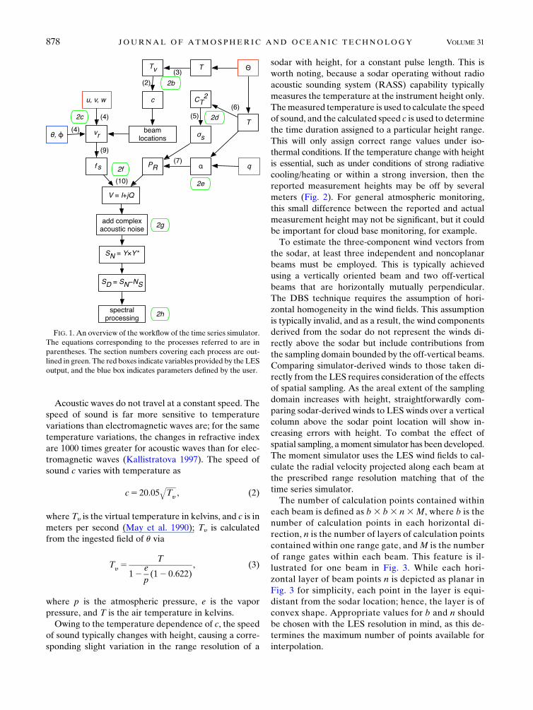
An overview of the workflow of the time series sim-

ulator is presented in Fig. 1. Equations corresponding to

each process are denoted in parentheses, and more de-

tail on each of these processes is presented within the

following subsections.

b. Beam locations

Many of the characteristics of the simulated sodar are

defined by the user, allowing for the emulation of dif-

ferent sodar models and the testing of operating strate-

gies. These include the placement of the sodar within the

LES domain and the number of independent beam di-

rections. The transmitted frequency, beamwidth, azi-

muth, and zenith angle of each beam are adjustable. The

desired approximate vertical range resolution is also set

by the user. The vertical range resolution should be

chosen such that it is larger than the vertical resolution

of the LES, for reasons detailed in section 5b. The pulse

duration t is calculated as

t52Dr

cref, (1)

where Dr is the desired range resolution and cref is

a reference speed of sound of 340m s21 (corresponding

to a temperature of 288K for dry air).

APRIL 2014 WA INWR IGHT ET AL . 877

Acoustic waves do not travel at a constant speed. The

speed of sound is far more sensitive to temperature

variations than electromagnetic waves are; for the same

temperature variations, the changes in refractive index

are 1000 times greater for acoustic waves than for elec-

tromagnetic waves (Kallistratova 1997). The speed of

sound c varies with temperature as

c5 20:05ffiffiffiffiffiffiffiTy

q, (2)

where Ty is the virtual temperature in kelvins, and c is in

meters per second (May et al. 1990); Ty is calculated

from the ingested field of u via

Ty 5T

12e

p(12 0:622)

, (3)

where p is the atmospheric pressure, e is the vapor

pressure, and T is the air temperature in kelvins.

Owing to the temperature dependence of c, the speed

of sound typically changes with height, causing a corre-

sponding slight variation in the range resolution of a

sodar with height, for a constant pulse length. This is

worth noting, because a sodar operating without radio

acoustic sounding system (RASS) capability typically

measures the temperature at the instrument height only.

Themeasured temperature is used to calculate the speed

of sound, and the calculated speed c is used to determine

the time duration assigned to a particular height range.

This will only assign correct range values under iso-

thermal conditions. If the temperature change with height

is essential, such as under conditions of strong radiative

cooling/heating or within a strong inversion, then the

reported measurement heights may be off by several

meters (Fig. 2). For general atmospheric monitoring,

this small difference between the reported and actual

measurement height may not be significant, but it could

be important for cloud base monitoring, for example.

To estimate the three-component wind vectors from

the sodar, at least three independent and noncoplanar

beams must be employed. This is typically achieved

using a vertically oriented beam and two off-vertical

beams that are horizontally mutually perpendicular.

The DBS technique requires the assumption of hori-

zontal homogeneity in the wind fields. This assumption

is typically invalid, and as a result, the wind components

derived from the sodar do not represent the winds di-

rectly above the sodar but include contributions from

the sampling domain bounded by the off-vertical beams.

Comparing simulator-derived winds to those taken di-

rectly from the LES requires consideration of the effects

of spatial sampling. As the areal extent of the sampling

domain increases with height, straightforwardly com-

paring sodar-derived winds to LES winds over a vertical

column above the sodar point location will show in-

creasing errors with height. To combat the effect of

spatial sampling, amoment simulator has been developed.

The moment simulator uses the LES wind fields to cal-

culate the radial velocity projected along each beam at

the prescribed range resolution matching that of the

time series simulator.

The number of calculation points contained within

each beam is defined as b 3 b 3 n 3M, where b is the

number of calculation points in each horizontal di-

rection, n is the number of layers of calculation points

contained within one range gate, andM is the number

of range gates within each beam. This feature is il-

lustrated for one beam in Fig. 3. While each hori-

zontal layer of beam points n is depicted as planar in

Fig. 3 for simplicity, each point in the layer is equi-

distant from the sodar location; hence, the layer is of

convex shape. Appropriate values for b and n should

be chosen with the LES resolution in mind, as this de-

termines the maximum number of points available for

interpolation.

FIG. 1. An overview of the workflow of the time series simulator.

The equations corresponding to the processes referred to are in

parentheses. The section numbers covering each process are out-

lined in green. The red boxes indicate variables provided by the LES

output, and the blue box indicates parameters defined by the user.

878 JOURNAL OF ATMOSPHER IC AND OCEAN IC TECHNOLOGY VOLUME 31

c. Radial velocity

Once the spatial location of each beam point has been

determined, the radial velocities at those points are de-

termined. The velocity components are first calculated at

the beam points by using trilinear interpolation on the

original fields of u, y, and w from the LES resolved on an

X 3 Y 3 Z numerical grid. The velocity components are

also interpolated in time between concurrent LES snap-

shots, to allow for spatial coherence between range gates.

The temporal interpolation is done using the time durations

assigned to each beam point during range determination.

The radial velocity is determined from the spatially

interpolated velocity components as

yr(u,f)5 u sinu sinf1 y sinu cosf1w cosu , (4)

where f and u are the azimuth and zenith angles of each

beam point, respectively.

d. Weighting functions

Two types of weighting functions are used in the

simulator. The function of the first type weights the ra-

dial velocity values based upon their location within the

beam and within the range gate. The beam-weighting

function employed is a multivariate normal distribution

with a mean of the center of the beam in the x and y

directions, and a standard deviation of the beamwidth.

Points near boresight have the maximum value of 0 dB,

with the value decreasing to23dB at specified beamwidth

distance. The range-weighting function is based on an

extended cosine pulse shape and also uses a maximum

value of 0 dB at the center range of each beam and

23 dB at the extremities of each range gate. The beam-

and range-weighting functions are combined to yield

one single volumetric weighting function with values

ranging from 0 to 26 dB. Weighting function of the sec-

ond type is based upon the backscattering intensity at

each beam point. The acoustic backscattering cross

section is calculated as

FIG. 2. (left) Four example vertical temperature profiles: isothermal, dry adiabatic, standard atmosphere, and

a low-level inversion. (right) Offset in actual height of range gates for the different temperature profiles if the

isothermal profile is assumed.

FIG. 3. The calculation points contained within each beam. (left)

The single range gate outlined in red is shown (right) in detail. Each

range gate contains b 3 b 3 n points at which calculations are

performed. Each of n layers of beam points contains points that are

equal in range from the sodar location. Thus, each layer is convex in

shape, while depicted as planar here for simplicity.

APRIL 2014 WA INWR IGHT ET AL . 879

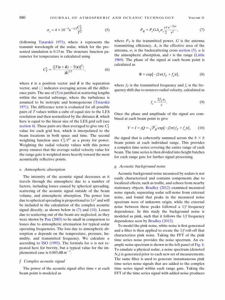
ss 5 43 1023l21/3C2T

T2(5)

(following Tatarskii 1971), where l represents the

transmit wavelength of the sodar, which for the pre-

sented simulation is 0.15m. The structure function pa-

rameter for temperature is calculated using

C2T 5

h[T(r1d)2T(r)]2ijdj2/3

, (6)

where r is a position vector and d is the separation

vector, and h�i indicates averaging across all the differ-

ence pairs. The use of (5) is justified at scattering lengths

within the inertial subrange, where the turbulence is

assumed to be isotropic and homogeneous (Tatarskii

1971). The difference term is evaluated for all possible

pairs of T values within a cube of equal size to the LES

resolution and then normalized by the distance d, which

here is equal to the linear size of the LES grid cell (see

section 4). These pairs are then averaged to give one C2T

value for each grid box, which is interpolated to the

beam locations in both space and time. The second

weighting function uses C2T /T

2 as a proxy for power.

Weighting the radial velocity values with this power

proxy ensures that the average radial velocity value for

the range gate is weighted more heavily toward the most

acoustically reflective points.

e. Atmospheric absorption

The intensity of the acoustic signal decreases as it

travels through the atmosphere due to a number of

factors, including losses caused by spherical spreading,

scattering of the acoustic signal outside of the beam

volume, and atmospheric absorption. The power loss

due to spherical spreading is proportional to 1/r2 andwill

be included in the calculation of the complex acoustic

signal directly, as shown below in (7) and (10). Losses

due to scattering out of the beam are neglected, as they

were shown by Pan (2003) to be small in comparison to

losses due to atmospheric attenuation for typical sodar

operating frequencies. The loss due to atmospheric ab-

sorption a depends on the temperature, pressure, hu-

midity, and transmitted frequency. We calculate a

according to ISO (1993). The formula for a is not re-

peated here for brevity, but a typical value for the im-

plemented case is 0.003 dBm21.

f. Complex acoustic signal

The power of the acoustic signal after time t at each

beam point is modeled as

PR 5PtGAess

ct

2

e22ar

r2, (7)

where PT is the transmitted power, G is the antenna

transmitting efficiency, Ae is the effective area of the

antenna, ss is the backscattering cross section (5), a is

the atmospheric absorption, and r is the range (Little

1969). The phase of the signal at each beam point is

calculated as

F5 exp[2j2p( fT 1 fs)t] , (8)

where fT is the transmitted frequency and fs is the fre-

quency shift due to nonzero radial velocity, calculated as

fs52fTyrc

. (9)

Once the phase and amplitude of the signal are com-

bined at each beam point to give

V5 I1 jQ5ffiffiffiffiffiffiffiffiffiPR

qexp[2j2p( fT 1 fs)t] , (10)

the signal that is coherently summed across the b 3 b

beam points at each individual range. This provides

a complex time series covering the entire range of each

beam. The time series is then divided into height batches

for each range gate for further signal processing.

g. Acoustic background noise

Acoustic background noise measured by sodars is not

easily characterized and contains components due to

localized effects, such as traffic, and echoes from nearby

stationary objects. Bradley (2012) examined measured

noise signals, separating sodar self-noise from external

noise, and found that peaks in the measured noise

spectrum were of unknown origin, while the external

noise between these peaks followed a 1/f frequency

dependence. In this study the background noise is

modeled as pink, such that it follows the 1/f frequency

dependence seen by Bradley (2012).

To model the pink noise, white noise is first generated

and a filter is then applied to create the 1/f roll-off that

characterizes pink noise. Taking the FFT of the pink

time series noise provides the noise spectrum. An ex-

ample noise spectrum is shown in the left panel of Fig. 4.

To emulate a physical sodar, a noise spectrum (denoted

NS) is generated prior to each new set of measurements.

The same filter is used to generate instantaneous pink

time series noise signals that are added to the complex

time series signal within each range gate. Taking the

FFT of the time series signal with added noise produces

880 JOURNAL OF ATMOSPHER IC AND OCEAN IC TECHNOLOGY VOLUME 31

the noisy Doppler spectrum (shown in black in Fig. 4a).

This completes the simulation of the signal.

h. Spectral processing

To process the synthesized signals, at each range gate

and beam, an FFT is taken of the complex time series

signal within that range, including both the back-

scattered acoustic signal and the background noise de-

scribed in the previous section. Multiplying the result of

the FFT (Y) by its conjugate (Y*) gives the Doppler

power spectrum, S 5 Y 3 Y*, for each range gate. The

signal processing is performed on a gate-by-gate basis

unlike a physical sodar, which typically operates on a full

vertical time series profile at once. The single-gate

processing was chosen purely to minimize computa-

tional expense in the model. Once a full scan containing

all the range gates and all beams is completed, a single

separate noise spectrum NS is generated. This single

noise spectrum emulates the noise spectra that a sodar

measures prior to each scan.

The single noise spectrum is subtracted from the noisy

Doppler spectrum S at each range gate to give an ef-

fective denoised Doppler spectrum SD (illustrated by

the black line in Fig. 4a). The same NS is used for each

range gate and beam within one scan. This allows us to

best emulate a physical sodar, which uses the measured

noise spectra obtained before each scan to remove noise

from all the received Doppler spectra within the scan.

Further signal processing is performed on SD. One of

the benefits of the simulator is that it allows for the

testing of different signal processing techniques on the

same atmospheric fields, enabling a fair comparison of

the different techniques.

Several signal processing techniques have been tested.

The one used in this study is outlined in Bradley (2008a)

and is illustrated in Fig. 4b. First, the peak of the

denoised Doppler spectrum is identified (vertical black

line of Fig. 4b). The frequency range to be used for de-

termination of the frequency shift is defined by a number

2m 1 1 frequency bins, centered upon the identified

peak, wherem is a positive integer. In this study we used

m5 5. The bounds of this frequency range aremarked in

Fig. 4b by dashed black lines. The frequency shift within

these bounds is determined by calculating the first mo-

ment of the spectrum via the use of a maximum likeli-

hood estimator that models the frequency spectrum as

normally distributed. Only spectra within the range

bounded by frequencies 2m 1 1 are used in the maxi-

mum likelihood estimator. This is done to reduce the

influence of background noise on determination of the

frequency shift. The frequency identified as the first

moment is shown on Fig. 4b in red. The frequency shift

for that range gate is simply the difference between the

first moment and the transmitted frequency.

The radial velocity for each range gate is retrieved by

rearranging (9) as

yr 5fsc

2fT, (11)

where c is calculated from (2) using the mean value of

temperature for beam points located within the con-

sidered range gate.

FIG. 4. (left) Example complete frequency spectrumwith included noise output by the simulator for an off-vertical

beam at a range of 165m (black line). The generated noise spectrum is shown in red. (right) Illustration of the spectral

processing. Points within a range of 2m1 1 frequency bins are used to calculate the Doppler frequency. Here,m5 5

and points in between the black dashed lines are included. The Doppler frequency used to calculate the radial

velocity is marked in red. The transmitted frequency is marked by the blue line.

APRIL 2014 WA INWR IGHT ET AL . 881

i. Postprocessing

If three or more independent noncoplanar beam di-

rections are used, then the wind components u, y, and w

can be retrieved from the radial velocity values. Typi-

cally, either three or five independent beams are used.

The radial velocities are related to the wind components

through (4), which for a five-beam retrieval can be

written as the system Cu 5 vr, where

C5

266666664

sinu1 sinf1 sinu1 cosf1 cosu1

sinu2 sinf2 sinu2 cosf2 cosu2

sinu3 sinf3 sinu3 cosf3 cosu3

sinu4 sinf4 sinu4 cosf4 cosu4

sinu5 sinf5 sinu5 cosf5 cosu5

377777775,

u5

264u

y

w

375 and vr 5

266666664

yr1

yr2

yr3

yr4

yr5

377777775

where fi and ui are the azimuth and the zenith angle for

beam i, respectively (Palmer et al. 1993). Once the cal-

culated radial velocities are known, the wind compo-

nents can be derived using the least squares solution of

the matrix equation

u5 (CTC)21CTvr . (12)

One of the advantages of the simulator is that it allows

for a variety of averaging periods to be used on the same

data, thus enabling an examination of the effect of the

averaging period on the derived wind fields. The time

averaging is performed by adding each individual

Doppler spectrum within the desired averaging period,

and recalculating the Doppler velocity based on the

technique depicted in Fig. 4.

3. Moment simulator

To evaluate the performance of the sodar simulator,

we wish to compare the derived three-component wind

field back to the original wind field from the LES output.

We chose to compare the results in two separate ways.

The first way is to compare the estimated wind field from

the simulator with wind values taken directly from the

LES output. This would be equivalent to comparing

winds from a sodar in a field campaign with winds

measured on an instrumented tower (with the neglect of

instrument error). One issue that can arise with this

validation method is that it is difficult to separate the

differences due to the spatial continuity assumption in-

herent in the DBS technique from the differences due

to the spectral processing. To help separate these

differences, we also estimate the wind fields using a

so-called moment simulator, briefly described in this

section.

The moment simulator uses the same beam locations

and weighting as the time series sodar simulator, but

it does not perform the spectral processing; rather, the

radial velocities contained within one range gate are

individually power weighted using C2T /T

2 and then

simply averaged to gain a representative value for that

gate. Thus, a comparison of the wind fields estimated

by the moment simulator and the virtual instrumented

tower would expose the differences that result solely

from the spatial averaging the DBS technique implies.

This is a useful technique because, as stated byAntoniou

et al. (2003), there is no feasible way to make point and

volume measurements directly comparable without

distributing many point measurement devices through-

out the volume encompassed by the sodar. While the

moment simulator does not allow for a direct compari-

son of results between the point and volume measure-

ments, it does allow for investigation of the biases

between these measurement approaches, which is useful

in itself. The challenges of comparing sodar- and in-

strumented mast-derived winds are investigated thor-

oughly by Bradley (2013), who states that the inherent

difference between vector and scalar averaging causes

an average root-mean-square (RMS) error in the mea-

sured winds of around 2%. Use of the DBS technique is

based on the assumption that each of the wind com-

ponents u, y, and w are constant across the region en-

compassed by the beam locations. Invalidity of this

assumption caused by nonuniform vertical velocities or

horizontal shear across the observed region can result in

a bias in the wind estimates (shown for wind profilers by

Koscielny et al. 1984).

Many field experiments have been performed to ver-

ify wind field measurements by sodars. Crescenti (1997)

summarized many of the earlier studies that compared

sodar-estimated winds with those from cup/vane ane-

mometers, sonic anemometers, and lidars. It was con-

cluded that Doppler sodars can reproduce reliable

profiles of the mean wind speed and direction, with

homogeneity in the wind fields leading to better com-

parisons between instruments. Inhomogeneity in the

boundary layer adds complication and hampers in-

terpretation of the resulting wind fields (Crescenti 1997).

These effects can be examined by intercomparison of

the winds from the virtual instrumented tower (LES)

and the moment simulator.

882 JOURNAL OF ATMOSPHER IC AND OCEAN IC TECHNOLOGY VOLUME 31

4. Large-eddy simulation data

The sodar simulator ingests turbulent flow fields

generated by an LES code. For this study we populated

the simulator with data from the University of Okla-

homa LES (OU-LES, Fedorovich et al. 2004a). The

simulation reproduced a developing convective bound-

ary layer and was performed in a domain of size

1.28 km3 1.28km3 1.5 kmwith a uniform grid spacing of

Dx5 Dy5 Dz5 5m. The lowest model level was located

at 2.5m above ground level. The employed subgrid tur-

bulence closure scheme is based upon Deardorff (1980).

The LES output used for this study corresponds to 1400–

1500 UTC 31 May 2009, in a domain centered upon the

Atmospheric Radiation Measurement Program Southern

Great Plains (ARM SGP) site in Lamont, Oklahoma.

The OU-LES was nudged incrementally at each time

step (about 1 s) using vertical profiles of virtual potential

temperature, water vapor mixing ratio, and the hori-

zontal wind components from the Rapid Update Cycle

(RUC; Benjamin et al. 1994), as described in Gibbs et al.

(2011). The surface fluxes were prescribed using tem-

porally interpolated sensible and latent heat fluxes from

the eddy correlation flux measurement system (ECOR;

Cook and Pekour 2008) at the ARM SGP site. The LES

output fields that are used in the simulator are the three-

dimensional fields of potential temperature Q; the wind

components, u, y, and w; and the water vapor mixing

ratio q.

The OU-LES has been tested extensively for the

convective boundary layer (CBL) conditions. Compar-

isons with experimental and numerical CBL data have

shown that it can realistically reproduce mean flow and

turbulence structure for clear CBL conditions (Fedorovich

et al. 2001, 2004b; Botnick and Fedorovich 2008). The

OU-LES output has previously been tested within the

framework of a boundary layer radar simulator (Scipi�on

et al. 2008), which allowed for testing of different scan-

ning strategies and signal processing techniques for

boundary layer radars, much like the present study does

for acoustic remote sensors.

5. Examples of using the sodar simulator

a. Experiment description

The sodar simulator has been tested on output from

the LES of the developing convective boundary layer

(see section 4). The simulator has many user inputs that

can be tailored to mirror existing systems. For this ex-

periment, the parameters were tailored tomatch aMetek

PCS.2000 sodar operated by theUniversity ofOklahoma.

For the test, a subset of LES output data from the sim-

ulationdescribed in section 4of size 400m3 400m3 600m

was used. One hour of data was used with the simulated

fields reported every 3 s. The transmitted sodar acoustic

frequency was set to 2300Hz. The maximum range was

set to 500m above ground level (AGL). The minimum

range is not directly defined by the user but is rather

determined from a defined transmit-to-receive delay that

is set at 0.1 s. This resulted in an effective minimum range

of 26m. The range resolution was 11.6m and 40 range

gates are simulated. Five beams were used with the four

off-vertical beams at 72.58 elevation angle, and the

beamwidth was 108. The azimuth angles of the four off-

vertical beams were multiples of 908. The fields of u, y, w,andQ were updated with each new beam direction at 3-s

intervals to give a complete set of measurements every

15 s. This timing is typical for the operational sodarwe are

simulating in this study. The number of points that are

equidistant in rangewithin each beam (b3 b) is set to 535. The number of ranges n contained within each range

gate is set to 640, which equates to a sampling frequency

close to 39 000Hz.

A sample of the numerically simulated CBL flow is

illustrated in Figs. 5 and 6. The boundary layer depth at

the early time of the simulation is around 300m, as in-

dicated in Fig. 5. The horizontal wind components u

and y are both seen to increase in magnitude above the

boundary layer. Beneath 300m, we see a pattern of

updrafts (positive w) and downdrafts (negative w), with

generally small magnitudes of w above the CBL top.

Figure 6 illustrates the strong spatial variability of u, y,

and w within the boundary layer, and it is clear that the

assumption that the wind components are homogeneous

across the area encompassed by the five sodar beams is

invalid.

b. Results

Results based on the radial velocity calculations for

the five beams of the sodar simulator are shown in Fig. 7.

The top panel shows a time-averaged vertical profile

of the RMS difference in the radial velocity of each

beam calculated by spectral processing as compared to

that from the moment simulator. One would expect the

RMS difference to increase with height due to the effect

of the assumption of spatial homogeneity inherent in

the DBS technique over an increasingly large area.

However, this does not seem to be the case. We see

that heights with increased RMS differences in radial

velocity—namely, close to the surface and at heights

close to the boundary layer top—are regions that exhibit

increased spatial heterogeneity of the three-dimensional

wind components. One may expect that for all heights

the RMS difference between the moment and spectrally

processed radial velocities would tend to zero over

a sufficiently long averaging period. We indeed see the

APRIL 2014 WA INWR IGHT ET AL . 883

RMS radial velocity difference decreasing with the av-

eraging period, but there seems to be a lower bound on

the RMS difference for some beams and heights. This is

most noticeable for beam 2 (the second panel in Fig. 7).

Particularly for heights between 300 and 350m, the RMS

difference does not significantly decrease as the averaging

period increases over 5min, indicating a systematic bias

of some kind.

The cause of this bias was thoroughly investigated. It

was found that the highest RMS differences in radial

velocity were collocated with range gates over which the

radial velocity changed the most over the height within

that range gate. If the radial velocity changes linearly (or

almost linearly) with height within the range gate, then

this introduces a linear variation in the frequency shift fsin (8), resulting in the complex voltage

V5ffiffiffiffiffiffiffiffiffiPR

qexpf2j2p[fT 1 ( fs 1At)]tg , (13)

where A represents the frequency slope caused by the

linear change in radial velocity over the depth of the

range gate. Taking the FFT of the signal in (13) does not

result in a spectral peak located exactly at fT 1 fs 1A/2,

which would be the instantaneous frequency at the

central timemoment within the FFT window, but results

in smearing of the peak in the FFT and phase distortion

(Masri and Bateman 1995).

A fundamental assumption when interpreting the FFT

results is that the signal statistics (up to second order) are

wide-sense stationary, that is, the signal is stationary over

the period that the FFT is taken. For sinusoidal signals of

the type considered in (10), it is assumed that the ampli-

tude and frequency remain constant within the FFT

window (in our case, the FFT window corresponds to

the time interval for which the signal is within one range

gate). The introduction of linear (or nonlinear) fre-

quency modulation obviously invalidates this assump-

tion. However, the FFT is the method used in most

operational sodars.

This frequency shift is not typically problematic for

operational sodars, as the perfectly linear frequency

modulation in the simulator is a result of the trilinear

interpolation of u, y, and w to the beam points. For an

operational sodar, the background and instrument noise

would typically overshadow the linear radial velocity

variation. For the sodar simulator, the effect of linear

frequency modulation is more marked at lower heights,

where the sodar beamwidth encompasses relatively few

LES grid points. At higher levels there is rarely perfect

linear frequency modulation due to radial velocity

contributions from an increased number of LES grid

points, which mitigates the frequency modulation effect

to some degree. For this reason, it is recommended that

LES output of sufficiently high spatial resolution to

provide contributions from more than two grid points,

even at the lowest range gates, is used.

One possible solution to overcome the linear varia-

tions in radial velocity is to include a contribution from

the subgrid turbulence kinetic energy E in the three-

dimensional wind components, as has been done for

radar simulators, (e.g., Cheong et al. 2008; Scipi�on et al.

2009). The authors tested this idea within the time series

simulator, but it was found to introduce large errors into

the simulation results. Investigation into the cause of the

subsequent errors revealed that at heights close to the

surface and the boundary layer height, values of E were

FIG. 5. Snapshots of the LES wind component fields at y5 0m. The areas encompassed by beams 1, 3, and 4 are overlaid. Presented data

illustrate the failure of the assumption that the three wind components are constant across the region defined by the beam locations.

884 JOURNAL OF ATMOSPHER IC AND OCEAN IC TECHNOLOGY VOLUME 31

as large as the resolved wind components, resulting in

large errors in the spectrally derived radial velocity.

In interpolating E down to a finer scale, we ignore the

inherent scale dependence of the resolved velocity field

and E in LES. One would expect that on a spatial scale

comparable to the beam point spacing used in the sim-

ulator (0.018m in the vertical), the subgrid contribution

would be significantly lower than the resolved con-

tribution. We suggest that future work include an in-

vestigation into the scaleability of resolved velocity

components and E down to small scale. This would al-

low the inclusion of contributions from E in the radial

velocity, which would compensate for the linear varia-

tion in radial velocity over a range gate.

Figure 8 illustrates the returned power from the

vertical beam in the sodar simulator, calculated as a

10-min average. This power is calculated as the peak

value of a sum of all the instantaneous frequency

spectra contained within the averaging period. We see

the decrease in power with range, as expected due to

the 1/r2 term in (7). During the first 20min of simula-

tion, power values are elevated close to the boundary

layer height due to increased spatial variation in tem-

perature there.

FIG. 6. Snapshots of the LES wind component fields at 20, 220, and 420m above ground level. Wind fields shown are from 30min into the

60-min simulation used for this experiment. The areas encompassed by each beam at the respective heights are overlaid.

APRIL 2014 WA INWR IGHT ET AL . 885

The main goal of this study was to evaluate the re-

cently developed time series sodar simulator using LES

output. As discussed in section 3, the performance of

operational sodars is often evaluated through compari-

son with in situ wind measurements. The simulator is

evaluated in this manner in Fig. 9. The figure illustrates

the wind speed and direction that would be calculated at

five different heights (40, 100, 200, 300, and 400m)

corresponding to measurement levels on a virtual in-

strumented (i.e., fitted with sonic anemometers) tower

whose base is exactly collocated with the simulated sodar.

The simulated wind measurements from the sonic an-

emometers are taken from the LES data in the desired

location, with no addition of instrument or background

noise. The left panels show results from the moment

simulator, and the differences between the moment

simulator and virtual tower data can be interpreted as

representative of the differences caused by point versus

spatially averaged measurements. Clearly, the time

series simulator (the right panels in Fig. 9) produces

greater outliers than the moment simulator in both

wind speed and direction. This is further evidenced by

the lower R2 values in both wind speed and direction

from the time series simulator than the moment simu-

lator (shown on Fig. 9). The top-right panel of Fig. 9

indicates that the time series sodar typically over-

estimates the wind speed as compared to the virtual

tower, where the wind speed values are calculated di-

rectly from the LES. Errors in the spectrally estimated

radial velocity caused by the assumption of stationarity

of the sign may also be contributing to this effect. The

wind speed generally increases with height, and as

discussed above, a linear increase in radial velocity

across a range gate can result in an increase in the

spectrally derived radial velocity.

6. Conclusions

In this study, we designed a sodar simulator that in-

gests numerically simulated turbulent flow fields. The

simulator has been developed in a way that many of its

operating parameters are defined by the user in order to

FIG. 7. (top) The RMS difference between radial velocity derived from the moment and spectral processing techniques, (middle) the

vertical beam, (bottom) the resulting RMS differences in derived values of u, y, and w. The different colored lines represent different

averaging periods.

886 JOURNAL OF ATMOSPHER IC AND OCEAN IC TECHNOLOGY VOLUME 31

facilitate comparisons with operational systems. LES

data from a clear CBL case were used in the study. To

evaluate the time series simulator, a moment simulator

was developed in parallel. The moment simulator uses

the same beam locations as the time series simulator, but

it does not include the spectral processing. In the mo-

ment simulator, the radial velocities contained within

a range gate are simply averaged to provide a represen-

tative velocity value. The use of the moment simulator

as a comparison tool ensures that any differences are

due to the sodar measurement and signal processing

technique and not caused by the invalidity of assuming

horizontal homogeneity of the three-component wind

field over the beams.

The performance of the time series simulator is con-

sistent with the moment simulator. Once again, the

RMS differences in u and y were highest at the boundary

layer top, where the wind components change the most

rapidly with height. As seen in Fig. 9, the derived wind

speed values from the time series simulator tend to be

higher than the ones measured at the virtual in-

strumented tower emulated through LES. We surmise

that this is partially due to the effect of trilinear in-

terpolation introducing an unphysical perfect linear

variation in radial velocity across the range gates. Ways

tomitigate this undesirable effect include the addition of

subgrid turbulence kinetic energy, although poor results

FIG. 8. Power from the vertical beam of the sodar simulator with an

arbitrary set zero power value.

FIG. 9. A comparison of the derived 10-min averaged wind speeds and directions from a virtual instrumented

tower, the moment simulator, and the time series simulator. The virtual tower data refer to five different heights,

while the moment and time series simulators are spatially averaged.

APRIL 2014 WA INWR IGHT ET AL . 887

from the initial testing of this theory suggest that further

investigation is required to determine an appropriate

scaling factor to use when interpolating subgrid values

down to scales considerably smaller than the grid spac-

ing of the LES.

The returned power modeled by the developed sodar

simulator appears realistic for a clear CBL case.

Overall, the sodar simulator provides a useful tool for

investigation of the way the boundary layer is viewed by

acoustic remote sensors. It allows for the emulation of

operational sodar systems and for the testing of different

scanning strategies and signal processing techniques on

the same turbulent flow data. It also provides a way to

compare wind data that would be obtained by point and

spatially averaged measurements in a variety of simu-

lated atmospheric environments.

Planned future work will be centered upon an in-

vestigation into an appropriate scaling for the inclusion

of spatially interpolated values of resolved velocity and

subgrid turbulence kinetic energy. This should allow for

a reduction in the RMS differences in wind components

between the moment- and spectrally derived values for

u, y, andw. It is also planned to test the simulator on LES

data for the stable boundary layer as well as to include

additional features in the simulator, such as the model-

ing of sodar-observed turbulent fluctuations of the ver-

tical velocity.

Acknowledgments. The National Science Foundation

(NSF) is acknowledged for the support of the reported

study through the Grant ATM-1016153. Three anony-

mous reviewers provided suggestions that substantially

improved the manuscript.

REFERENCES

Antoniou, I., H. E. Joergensen, F. Ormel, S. Bradley, S. von

H€unerbein, S. Emeis, and G. Warmbier, 2003: On the theory

of sodar measurement techniques. Risø DTU National Lab-

oratory Rep. Risø-R-1410 (EN), 60 pp.

Balsley, B. B., and K. Gage, 1982: On the use of radars for oper-

ational profiling. Bull. Amer. Meteor. Soc., 63, 1009–1018,

doi:10.1175/1520-0477(1982)063,1009:OTUORF.2.0.CO;2.

Benjamin, S. G., K. J. Brundage, and L. L. Morone, 1994: Im-

plementation of the Rapid Update Cycle. Part I: Analysis/model

description. NOAA/NWS Tech. Procedures Bull. 416, 16 pp.

Botnick, A. M., and E. Fedorovich, 2008: Large eddy simulation of

atmospheric convective boundary layer with realistic envi-

ronmental forcings. Quality and Reliability of Large-Eddy

Simulations, J. Meyers, B. Geurts, and P. Sagaut, Eds.,

ERCOFTAC Series, Vol. 12, Springer Verlag, 193–204.

Bradley, S. G., 1999: Use of coded waveforms for sodar systems.

Meteor. Atmos. Phys., 71, 15–23, doi:10.1007/s007030050039.

——, 2008a: Atmospheric Acoustic Remote Sensing. CRC Press,

296 pp.

——, 2008b: Wind speed errors for lidars and sodars in complex

terrain. IOP Conf. Ser.: Earth Environ. Sci., 1, 012061,

doi:10.1088/1755-1315/1/1/012061.

——, 2012: The noise part of sodar signal-to-noise. Extended

Abstracts, 16th Int. Symp. for the Advancement of Boundary-

Layer Remote Sensing, Boulder, CO, ISARS, 271–274.

[Available online at http://www.esrl.noaa.gov/psd/events/2012/

isars/pdf/isars2012-abstractVolume.pdf.]

——, 2013: Aspects of the correlation between sodar and mast

instrument winds. J. Atmos. Oceanic Technol., 30, 2241–2247,

doi:10.1175/JTECH-D-12-00256.1.

Capsoni, C., M. D’Amico, and R. Nebuloni, 2001: A multipa-

rameter polarimetric radar simulator. J. Atmos. Oceanic

Technol., 18, 1799–1809, doi:10.1175/1520-0426(2001)018,1799:

AMPRS.2.0.CO;2.

Cheong, B. L., M. W. Hoffman, and R. D. Palmer, 2004: Efficient

atmospheric simulation for high-resolution radar imaging ap-

plications. J. Atmos. Oceanic Technol., 21, 374–378, doi:10.1175/

1520-0426(2004)021,0374:EASFHR.2.0.CO;2.

——, R. D. Palmer, and M. Xue, 2008: A time series weather

radar simulator based on high-resolution atmospheric mod-

els. J. Atmos. Oceanic Technol., 25, 230–243, doi:10.1175/

2007JTECHA923.1.

Clothiaux, E., T. Ackerman, and D. Babb, 1996: Ground-based

remote sensing of cloud properties using millimeter-wave ra-

dar. Radiation and Water in the Climate System: Remote

Measurements, E. Raschke, Ed., NATOASI Series I, Vol. 45,

Springer, 323–366.

Cook, D. R., and M. S. Pekour, 2008: Eddy correlation flux mea-

surement system handbook. DOE Tech. Rep. DOE/SC-

ARM/TR-05, 15 pp. [Available online at http://www.wmo.

int/pages/prog/gcos/documents/gruanmanuals/Z_instruments/

ecor_handbook.pdf.]

Crescenti, G. H., 1997: A look back on two decades of Doppler

sodar comparison studies. Bull. Amer. Meteor. Soc., 78, 651–

673, doi:10.1175/1520-0477(1997)078,0651:ALBOTD.2.0.CO;2.

Deardorff, J. W., 1980: Stratocumulus-capped mixed layer derived

from a three-dimensional model. Bound.-Layer Meteor., 18,

495–527, doi:10.1007/BF00119502.

Fedorovich, E., F. T. M. Nieuwstadt, and R. Kaiser, 2001: Nu-

merical and laboratory study of horizontally evolving con-

vective boundary layer. Part I: Transition regimes and

development of the mixed layer. J. Atmos. Sci., 58, 70–86,

doi:10.1175/1520-0469(2001)058,0070:NALSOA.2.0.CO;2.

——, R. Conzemius, and D. Mironov, 2004a: Convective en-

trainment into a shear-free, linearly stratified atmosphere:

Bulk models reevaluated through large eddy simulations.

J. Atmos. Sci., 61, 281–295, doi:10.1175/1520-0469(2004)061,0281:

CEIASL.2.0.CO;2.

——, and Coauthors, 2004b: Entrainment into sheared convec-

tive boundary layers as predicted by different large eddy

simulation codes. Preprints, 16th Symp. on Boundary Layers

and Turbulence, Portland, ME, Amer. Meteor. Soc., P4.7.

[Available online at https://ams.confex.com/ams/BLTAIRSE/

techprogram/paper_78656.htm.]

Gibbs, J. A., E. Fedorovich, andA.M. J. van Eijk, 2011: Evaluating

Weather Research and Forecasting (WRF) model predictions

of turbulent flow parameters in a dry convective boundary

layer. J. Appl. Meteor. Climatol., 50, 2429–2444, doi:10.1175/

2011JAMC2661.1.

Greenhut, G. K., and G. Mastrantonio, 1989: Turbulence ki-

netic energy budget profiles derived from Doppler sodar

888 JOURNAL OF ATMOSPHER IC AND OCEAN IC TECHNOLOGY VOLUME 31

measurements. J. Appl. Meteor., 28, 99–106, doi:10.1175/

1520-0450(1989)028,0099:TKEBPD.2.0.CO;2.

ISO, 1993: Acoustics—Attenuation of sound during propagation

outdoors—Part 1: Calculation of the absorption of sound by

the atmosphere. International Standards Organization Rep.

ISO9613-1:1993(E), 26 pp.

Jung, Y., G. Zhang, and M. Xue, 2008: Assimilation of simulated

polarimetric radar data for a convective storm using the en-

semble Kalman filter. Part I: Observation operators for re-

flectivity and polarimetric variables. Mon. Wea. Rev., 136,

2228–2245, doi:10.1175/2007MWR2083.1.

Kallistratova, M. A., 1997: Physical grounds for acoustic remote

sensing of the boundary layer. Acoustic Remote Sensing Ap-

plication, S. P. Singal, Ed., Lecture Notes in Earth Sciences,

Vol. 69, Springer Verlag, 3–34.

——, and R. L. Coulter, 2004: Application of sodars in the study

and monitoring of the environment.Meteor. Atmos. Phys., 85,

21–37.

Koscielny, A. J., R. J. Doviak, and D. S. Zrni�c, 1984: An evalu-

ation of the accuracy of some radar wind profiling tech-

niques. J. Atmos. Oceanic Technol., 1, 309–320, doi:10.1175/

1520-0426(1984)001,0309:AEOTAO.2.0.CO;2.

Little, C. G., 1969: Acoustic methods for the remote probing of the

lower atmosphere. Proc. IEEE, 57, 571–578, doi:10.1109/

PROC.1969.7010.

Masri, P., and A. Bateman, 1995: Identification of nonstationary

audio signals using the FFT, with application to analysis-based

synthesis of sound. IEEE Colloquium on Audio Engineering

Digest, Vol. 1995/089, IEEE, 11/1–11/6.

May, P. T., R. G. Strauch, K. P. Moran, and W. L. Ecklund, 1990:

Temperature sounding by RASS with wind profiler radars: A

preliminary study. IEEE Trans. Geosci. Remote Sens., 28, 19–

28, doi:10.1109/36.45742.

May, R. M., M. I. Biggerstaff, and M. Xue, 2007: A Doppler

radar emulator with an application to the detectability of

tornadic signatures. J. Atmos. Oceanic Technol., 24, 1973–

1996, doi:10.1175/2007JTECHA882.1.

Muschinski, A., P. P. Sullivan, D. B. Wuertz, R. J. Hill, S. A. Cohn,

D. H. Lenschow, and R. J. Doviak, 1999: First synthesis of

wind-profiler signals on the basis of large-eddy simulation

data. Radio Sci., 34, 1437–1459, doi:10.1029/1999RS900090.

Neff, W. D., 1988: Observations of complex terrain flows using

acoustic sounders: Echo interpretation. Bound.-Layer Me-

teor., 42, 207–228, doi:10.1007/BF00123813.

Palmer,R.D.,M. F. Larsen,E. L. Sheppard, S. Fukao,M.Yamamoto,

T. Tsuda, and S. Kato, 1993: Poststatistic steering wind esti-

mation in the troposphere and lower stratosphere.Radio Sci.,

28, 261–271, doi:10.1029/93RS00279.

Pan,N., 2003: Excess attenuation of an acoustic beam by turbulence.

J. Acoust. Soc. Amer., 114, 3102–3111, doi:10.1121/1.1628679.Scipi�on, D. E., A. M. Botnick, R. D. Palmer, P. B. Chilson, and

E. Fedorovich, 2008: Inter-comparison of retrieved wind fields

from large-eddy simulations and radar measurements in the

convective boundary layer. IOP Conf. Ser.: Earth Environ.

Sci., 1, 012003, doi:10.1088/1755-1315/1/1/012003.

——,R.D. Palmer, P. B. Chilson, E. Fedorovich, andA.M.Botnick,

2009: Retrieval of convective boundary layer wind fields sta-

tistics from radar profiler measurements in conjunction with

large eddy simulations. Meteor. Z., 18, 175–187, doi:10.1127/

0941-2948/2009/0371.

Soler, M. R., J. Hinojosa, M. Bravo, D. Pino, and J. V.-G. de

Arellano, 2003: Analyzing the basic features of different

complex terrain flows by means of a Doppler sodar and a nu-

merical model: Some implications for air pollution problems.

Meteor. Atmos. Phys., 85, 141–154.Tatarskii, V. I., 1971: The Effects of the Turbulent Atmosphere on

Wave Propagation. Kefer Press, 472 pp.

Yu, T.-Y., and R. D. Palmer, 2001: Atmospheric radar imaging

using spatial and frequency diversity. Radio Sci., 36, 1493–1504, doi:10.1029/2000RS002622.

APRIL 2014 WA INWR IGHT ET AL . 889