Citation: Mukha, T.; Almeland, S.K.;

Bensow, R.E. Large-Eddy Simulation

of a Classical Hydraulic Jump:

Influence of Modelling Parameters on

the Predictive Accuracy. Fluids 2022,

7, 101. https://doi.org/10.3390/

fluids7030101

Academic Editors: Federico Piscaglia

and Jérôme Hélie

Received: 31 January 2022

Accepted: 25 February 2022

Published: 7 March 2022

Publisher’s Note: MDPI stays neutral

with regard to jurisdictional claims in

published maps and institutional affil-

iations.

Copyright: © 2022 by the authors.

Licensee MDPI, Basel, Switzerland.

This article is an open access article

distributed under the terms and

conditions of the Creative Commons

Attribution (CC BY) license (https://

creativecommons.org/licenses/by/

4.0/).

fluids

Article

Large-Eddy Simulation of a Classical Hydraulic Jump:Influence of Modelling Parameters on the Predictive AccuracyTimofey Mukha 1,2,* , Silje Kreken Almeland 3 and Rickard E. Bensow 1

1 Department of Mechanics and Maritime Sciences, Chalmers University of Technology,SE-412 96 Gothenburg, Sweden; rickard.bensow@chalmers.se

2 Department of Engineering Mechanics, KTH Royal Institute of Technology, SE-100 44 Stockholm, Sweden3 Department of Civil and Environmental Engineering, Norwegian University of Science and Technology,

NO-7491 Trondheim, Norway; silje.k.almeland@ntnu.no* Correspondence: tmu@kth.se

Abstract: Results from large-eddy simulations of a classical hydraulic jump at inlet Froude numbertwo are reported. The computations were performed using the general-purpose finite-volume-basedcode OpenFOAM®, and the primary goal was to evaluate the influence of the modelling parameterson the predictive accuracy, as well as establish the associated best-practice guidelines. A benchmarksimulation was conducted on a grid with a 1 mm-cell-edge length to validate the solver and providea reference solution for the parameter influence study. The remaining simulations covered differentselections of the modelling parameters: geometric vs. algebraic interface capturing, three meshresolution levels, and four choices of the convective flux interpolation scheme. Geometric interfacecapturing led to better accuracy, but deteriorated the numerical stability and increased the simulationtimes. Interestingly, numerical dissipation was shown to systematically improve the results, bothin terms of accuracy and stability. Strong sensitivity to the grid resolution was observed directlydownstream of the toe of the jump.

Keywords: hydraulic jump; large-eddy simulation; CFD; OpenFOAM

1. Introduction

A hydraulic jump is an abrupt change in the water depth accompanying the transitionof the flow from supercritical to subcritical. This transition causes energy dissipation,which defines the application of hydraulic jumps in engineering. In fact, according to [1],hydraulic jumps are the most commonly used energy dissipators in hydraulic structures.However, the hydraulic jump is also a natural environmental phenomenon, occurring inrivers and bays. This motivates the significant attention this class of flows has received fromthe scientific community. Hydraulic jumps have been the subject of a multitude of studies,both experimental and numerical; recent reviews can be found in [2,3]. Most works focuseson the so-called “classical” hydraulic jump (CHJ), which occurs in a smooth horizontalrectangular channel.

An illustration of the air-water interface in a CHJ is shown in Figure 1. The topologyof the interface is complex and rapidly evolving, which can be fully appreciated by lookingat the animations found in the archive published alongside this article (see the DataAvailability Statement). The interface dynamics are driven by a recirculating motion—theso-called roller—which leads to overturning waves occurring across the jump.

Consequently, a significant amount of air is entrained. A detailed discussion of theentrainment mechanism can be found in [4]. The flow in the jump is also highly turbulent,with a turbulent shear layer forming below the roller and interacting with it.

The main physical parameter of the CHJ is the inlet Froude number, Fr1, computedbased on the water inlet velocity, U1, and its depth, d1. Several classifications of the jump’sbehaviour based on Fr1 can be found in the literature; see [2] and the references therein.

Fluids 2022, 7, 101. https://doi.org/10.3390/fluids7030101 https://www.mdpi.com/journal/fluids

Fluids 2022, 7, 101 2 of 22

The most stable CHJs occur when Fr1 ∈ [4, 9]. The rate of air entrainment also depends onthe Froude number, and at higher Fr1, the level of aeration increases. Here, we considereda jump at Fr1 = 2, which corresponds to the “weak jump” [5] regime. It is characterised bya relatively thick jet at low velocity entering the jump and a relative energy loss of about7% [6].

Figure 1. Classical hydraulic jump at Fr1 = 2; a snapshot of the air–water interface.

In spite of the flow’s complexity, given the parameters of the inflow, some of itsproperties can be easily derived analytically based on control volume analysis; see e.g., [7](p. 250). This includes the water depth after the jump, d2 = 0.5d1

((1 + 8Fr2

1)0.5 − 1

).

From a numerical perspective, the CHJ represents an extremely challenging test ofpredictive capabilities for multiphase modelling approaches. A suitable model should beable to capture fast and complex topology changes taking place across a wide range ofspatial scales. Accurate turbulence modelling is also necessary and, in particular, the possi-bility to properly account for its interaction with the multiphase structures. On the otherhand, the geometric simplicity of the case makes mesh generation easy, and the abundanceof published experimental data makes validation easier. Furthermore, data from directnumerical simulation (DNS) [4] are also available.

A compilation of previous numerical studies of the CHJ, classified by turbulencemodelling approach, and also Fr1, can be found in [3]. At the lowest level of fidelity, thereare works where the jump is simulated using one-dimensional Boussinesq equations; see [8].However, the majority of works are based on two-equation Reynolds-averaged Navier–Stokes (RANS) turbulence models and the volume of fluid (VoF) method for capturingthe interface. Note that in RANS, it is assumed that there is a clear scale separationbetween the modelled turbulent motion and other types of unsteadiness. In the caseof a CHJ, this is unlikely to take place due to the direct interaction between turbulenceand multiphase structures, e.g., entrained bubbles. Generally, it is unclear whether thetopological changes in the flow occur significantly slower than the integral time scalesof turbulence. A possibility for resolving this inconsistency is keeping the resolutioncoarse enough for the interface to remain steady and introduce an explicit model for airentrainment, as performed in [9]. However, these theoretical difficulties do not imply thatRANS cannot be used to obtain useful results. On the contrary, as summarised in [3], RANSis capable of predicting d2, the mean location of the interface, and the length of the rollerwith a <5% relative error.

In order to obtain new physical insights and obtain an accurate picture of the turbulentmotion inside the jump, scale-resolving turbulence modelling approaches can be used. Onlya few studies have reported results from such simulations. The DNS by Mortazavi et al. [4]was already mentioned above and represents an important milestone. In [10,11], detached-eddy simulation (DES) was used. A detailed analysis of the flow was given; in particular,a quadrant decomposition of the turbulent shear stress was considered, as well as high-order statistical moments of the velocity field. A large-eddy simulation (LES) of a CHJ wasconducted as part of the study by Gonzalez and Bombardelli, which also included RANSsimulations [12]. Unfortunately, due to the reference being a short conference abstract, theresults were only discussed superficially. In [13], the authors reported on an unsuccessfulattempt to conduct an LES: the location of the jump could not be stabilised. Finally, in [9],which was already mentioned in the context of RANS, results from DES modelling were

Fluids 2022, 7, 101 3 of 22

also discussed. However, the simulation in question was not a DES in the classical sense,i.e., not a fully resolved LES outside the RANS region. Instead, a rather coarse mesh wasused, and an air entrainment model was employed. Nevertheless, this DES yielded moreaccurate results than the corresponding RANS.

With the increase of available computing power, it can be expected that LES and itshybrids will find wider adoption in hydraulic engineering in the near future. This transitionis already well under way in, for example, the automotive and aerospace industries. Froma practical perspective, an important step is to establish guidelines for the selection ofthe most important LES modelling parameters and understand the limitations in termsof accuracy that can be achieved at a given computational cost. Of immediate interestis to consider the particular case of solvers based on finite-volume discretisation, sincethese are currently the workhorse of industrial computational fluid dynamics. In thisnumerical framework, the two arguably most important LES input parameters are thedensity of the grid and the numerical scheme used for interpolating convective fluxes. Bothcontrol the capability of the LES to resolve turbulent structures, as well as the stabilityof the simulation. In the case of multiphase flow, the choice of the interface-capturingscheme is also important. The goal of this paper was to quantify the effects of these threeparameters on the various quantities of interest. To that end, results from an LES campaign,consisting of 25 simulations of a CHJ at Fr1 = 2, are presented. This included a high-fidelitysimulation with a similar resolution level as the DNS in [4]. In total, the campaign coveredfour different mesh resolution levels and two VoF approaches: algebraic and geometric.The diffusivity of the convective flux interpolation scheme was also controlled, and fourdiffusivity levels were considered. All the simulation results, including ready-to-runsimulation cases, are made available as a supplementary dataset (see the Data AvailabilityStatement).

The remainder of the article is structured as follows. Section 2 presents the compu-tational fluid dynamics methods used in the paper. The setup of the CHJ simulations ispresented in Section 3. The results of the simulation campaign are shown and analysed inSection 4. Finally, concluding remarks are given in Section 5.

2. Computational Fluid Dynamics Methods2.1. Governing Equations

The volume of fluid (VoF) method [14] was used to simulate the flow. Accordingly,a single set of conservation equations was solved for both fluids, and the phase wasdistinguished based on the values of the volume fraction of the liquid, α. The momentumand continuity equations read as follows,

∂ρui∂t

+∂

∂xj

(ρuiuj

)= −

∂pρgh

∂xi− gixi

∂ρ

∂xi+

∂

∂xj

(µ

(∂ui∂xj

+∂uj

∂xi

))+ fs, (i = 1, 2, 3) (1)

∂uj

∂xj= 0. (2)

Here, summation is implied for repeated indices, ui is the velocity, ρ is the density, µ isthe dynamic viscosity, gi is the standard acceleration due to gravity, pρgh = p− ρgixi is thedynamic pressure, and fs is the surface tension force. The latter was accounted for usingthe continuous force model [15]:

f si = σκ

∂α

∂xi. (3)

Here, σ is the surface tension coefficient and κ = ∂n fi /∂xi is the curvature of the

interface between the two phases, where n fi is the interface unit-normal, which is computed

as follows,

n fi =

∂α

∂xi

/(∣∣∣∣ ∂α

∂xi

∣∣∣∣+ δN

). (4)

Fluids 2022, 7, 101 4 of 22

Here, δN is a small number added for the sake of numerical stability.Equations (1) and (2) must be complemented with an interface-capturing approach in

order to compute the distribution of α. Methodologies for this are discussed in the nextsubsection. Given the values of α, the local material properties of the fluid are computed as:

ρ = αρ1 + (1− α)ρ2, (5)

µ = αµ1 + (1− α)µ2, (6)

where the indices 1 and 2 are used to refer to the liquid and gas properties, respectively.

2.2. Interface Capturing Methods

As discussed above, it is necessary to introduce a method for computing the evolutionof α, i.e., capture the location of the interface between the two fluids. Here, two differentapproaches to this were considered. The first is algebraic, meaning that a transport equationfor α is solved:

∂α

∂t+

∂ujα

∂xj+

∂

∂xj

(ur

j (1− α)α)= 0. (7)

The last term in the equation is artificial, and its purpose is to introduce additionalcompression of the interface. To that end, the direction of ur

i is aligned with the interface

normal, n fi . The magnitude of ur

i is defined as Cα|ui|, where Cα = 1 is an adjustable constant.Special treatment of the convective term in (7) is necessary in order to ensure that α is

bound to values between 0 and 1. Typically, a total-variation diminishing (TVD) schemeis chosen to compute the convective flux, but this can be insufficient because the TVDproperty of such schemes is, in fact, only strictly valid for one-dimensional problems. Anadditional flux-limiting technique, referred to as MULES, was used to rectify this. Whilewe omit discussing MULES in detail and instead refer the reader to [16], we note that it isbased on the idea of flux-corrected transport and the work of Zalesak [17]. It should alsobe mentioned that two variations of MULES are available in OpenFOAM®, explicit andsemi-implicit. Using the latter sometimes allows keeping the simulation stable for CFLnumbers larger than one.

The second approach belongs to the class of geometric VoF methods and is referredto as isoAdvector. The details of isoAdvector can be found in [18]; here, we provide abrief summary of the key steps of the algorithm. In contrast to algebraic VoF, here, thesurface of the interface is explicitly reconstructed at each time step. Within each cell, it isrepresented by a plane, and the reconstruction algorithm ensures that it divides the cellvolume consistently with the local value of α. To predict the location of the interface atthe next time step, it is advected along the direction of the interface normal. For each cell,the advection velocity is obtained using linear interpolation from the vertices of the cellonto the centroid of the interface-plane. Then, based on the predicted new location of theinterface, the change in α is computed.

Comparing the two approaches, one can generally say that geometric VoF can beexpected to be more accurate, yet more computationally demanding. Quantifying thesedifferences for the case of the hydraulic jump was one of the goals of the present paper.A significant drawback of the algebraic VoF is the necessity to choose the convectionscheme for α, which can have a large influence on the results. Selecting the values of modelconstants, such as Cα, also represents a difficulty.

2.3. Numerical Methods

The computations were performed using the open-source CFD software OpenFOAM®

Version 1806. This code is based on cell-centred finite-volume discretisation, whichcan currently be considered standard for industrial CFD. Two solvers distributed withOpenFOAM® were employed, corresponding to the two VoF methodologies discussedabove. For algebraic VoF, the solver interFoam was used, whereas isoAdvector was im-plemented in the interIsoFoam solver. Here, we omit the particulars regarding the solver

Fluids 2022, 7, 101 5 of 22

algorithms, but note that they are based on the PISO [19] pressure–velocity coupling proce-dure. For a detailed discussion, we refer the reader to the following thesis works [16,20].

A key component of the finite-volume method is the spatial interpolation and timeintegration schemes. For spatial interpolation, the goal is to obtain the values of theunknowns at the cell face centroids based on the values at the centroids of the cells. Themost trivial choice is using linear interpolation, which is second-order accurate. Thisscheme can be applied to interpolation of diffusive fluxes without negative side-effects.Unfortunately, when applied to convective fluxes, linear interpolation leads to a dispersiveerror. In spite of this, in single-phase LES and DNS, it is common practice to use this schemeanyway because the high density of the mesh, in combination with a small time step, allowsavoiding any significant contamination of the solution. On the other hand, in industrialflow simulations, it is quite common to use a second-order upwind scheme. Although alsounbounded, the error introduced by this scheme is dominated by a dissipative term, whichfacilitates the stability of the simulation, but negatively affects the capability to resolvesmall-scale turbulent motions. In this work, a linear blending of these two interpolationschemes was considered. The following weights for the linear upwind scheme were tested:10%, 25%, 50%, and 100%. For simplicity, this weight is referred to as “the amount ofupwinding” in the remainder of the paper.

For time integration, both solvers have the option of using a first-order implicit Eulerscheme. In interFoam, the Crank–Nicholson scheme can also be used, as well as a linearblending of Crank–Nicholson and Euler. In interIsoFoam, one can instead use a second-order accurate backward-differencing scheme. Unfortunately, it was only possible to keepthe simulations stable using the Euler scheme. However, since the employed time step sizeswere kept low, it was anticipated that the numerical errors would be dominated by thespatial interpolation errors, whereas the time-integration error would play a smaller role.

Finally, in the case of MULES, a scheme has to be chosen for the convection of α. Here,a TVD scheme using the van Leer limiter was selected to that end; see [21] (p. 170), for thedefinition. The selected limiter results in a more diffusive scheme than some alternatives,but here, the artificial compression term in (7) remedied that.

2.4. Turbulence Modelling

In order to obtain the governing equations for LES based on the employed two-phaseflow model, spatial filtering should be formally applied to Equations (1) and (2), as wellas (7) in the case of algebraic VoF. Following standard practice, we used implicitly filteredLES, letting the finite-volume grid act as the spatial filter. The associated filter size wasequal to the cubic root of the local computational cell volume.

Filtering led to the appearance of the subgrid stress (SGS) term in the momentumEquation (1). Several models are available for this term, the majority based on the Boussi-nesq approximation, meaning that the stress is assumed to have the same structure as theviscous stress. Unfortunately, the existing closures were designed for single-phase flowsand do not account for the interaction effects between multiphase and turbulent structures.Detailed investigations of the impact of this on the predictive accuracy have not yet beenreported in the literature. Here, we considered the effect of SGS modelling by comparingsimulation results obtained with the WALE model [22] and without explicit SGS modelling.The results are available in Appendix A, and the effect of the SGS model can be seen to bemarginal. This is in line with the authors’ previous experience with finite-volume solvers,particularly when relatively dissipative numerical schemes are employed. Numerical dissi-pation may be comparable in magnitude to that produced by the SGS model, and havingboth present in the simulation may lead to the deterioration of the accuracy. Further resultscomparing the performance of SGS models in OpenFOAM for single-phase flows can befound in [23]. In that study, none of the SGS models considered managed to improve uponnot using an explicit model. Based on these considerations and the results in Appendix A,we chose to run the simulations without SGS modelling.

Fluids 2022, 7, 101 6 of 22

2.5. Instability Sources in VoF Simulations

Compared to single-phase LES, numerical stability in LES-VoF simulations can besignificantly harder to achieve. As discussed in Section 4, for certain combinations ofthe grid resolution, VoF methodology, and amount of upwinding, the CHJ simulationsdiverged. It is therefore appropriate to briefly review the main additional sources ofnumerical instability intrinsic to the considered multiphase modelling approach.

The continuous force model (see Equations (3) and (4)) used for the surface tensionforce computation can lead to parasitic currents across the interface between the phases. Anillustration of such currents produced in an interFoam simulation of a single rising bubblecan be found in [24]. The source of the currents was the numerical imbalance between thepressure gradient across the interface and the surface tension. When the velocity of theparasitic current becomes large, the simulation may crash. Interestingly, in [25], the authormentioned that the sharper interface obtained using isoAdvector actually increased themagnitude of the parasitic currents.

A multitude of improvements to the continuous force model have been proposed,ranging from more accurate curvature estimation algorithms to more robust discrete han-dling of the balance between pressure and surface tension forces; see, for example, [26]. Animproved interface reconstruction algorithm for the herein-used geometric VoF methodwas recently validated in [27]. The results showed a reduction in parasitic current in thecanonical benchmark case of a stagnant bubble in a quiescent liquid. In [28], the authorspresented a library, which includes several new surface tension models for OpenFOAM.Unfortunately, these developments were not yet available at the time we conducted thesimulations.

The second source of instabilities was the treatment of the gravity term in the momen-tum Equation (1). When a segregated pressure–velocity coupling algorithm, such as PISO,is used, a numerical imbalance between the dynamic pressure gradient and the densitygradient terms can occur, which will be compensated by an acceleration of the fluid [29].This can lead to a strong increase of the velocity magnitude in the gas above the interface,due to its low density. For this reason, it is not uncommon to artificially increase the densityof the gas to facilitate stability.

The crucial practical consequence of the above is that one does not necessarily obtaina more stable simulation by refining the grid and using a more accurate interface-capturingapproach. This is very different from single-phase incompressible LES, in which dampeningnumerical instabilities by using a denser grid or a smaller time step is a common strategy.It should also be mentioned that it is not possible to predict when the discussed instabilitieswill take place. Some of the CHJ simulations conducted as part of this study were wellunder way when the destabilizing velocity overshoots occurred, leading to the loss of tensof thousands of core-hours worth of computing time. An even more unfortunate scenariois when a very strong spurious current takes place, but no crash occurs. The simulationfinished, but the results were unpublishable because the computed statistical momentsof velocity were contaminated. In our simulations, the solver would sometimes exhibitsurprising resilience and survive currents that were 3 orders of magnitude stronger thanthe characteristic velocity scale of the flow. It is therefore recommended to closely monitorthe maximum velocity values in the course of the simulation.

3. Simulation Setup

The setup of the simulation was similar to that used in the DNS by Mortazavi et al. [4].An overview of the computational domain, as well as the boundary conditions can be foundin Figure 2, and Table 1 contains a full list of the setup parameters. The main difficulty insetting up a hydraulic jump simulation is obtaining a stable jump positioned sufficientlyfar away from the inlet and outlet boundaries of the domain. A common approach tofacilitating the formation of the jump is by introducing a vertical barrier—a weir—somedistance upstream of the outlet; see, e.g., [10,30,31]. In other works [1,4,32], including the

Fluids 2022, 7, 101 7 of 22

reference DNS, the jump was controlled by the boundary condition at the outlet of thedomain. The particular condition enforced varies among the studies.

Figure 2. Simulation setup.

Table 1. Simulation parameters.

Property Value

Water inlet height, d1 0.059 mWater height post-jump, d2 0.140 mDomain length, Lx 2.05 m, ≈34.75d1Domain height, Ly 0.47355 m, ≈8d1Domain width, Lz 0.2478 m/0.4956 m, 4.2d1/8.4d1Weir height, Hw 0.02225 mWeir length The edge-length of the computational cell, ∆xDistance from the weir to the outlet, Lw 0.2 mLiquid density, ρ1 997.3 kg/m3

Gas density, ρ2 1.20012 kg/m3

Density ratio, ρ1/ρ2 831Liquid kinematic viscosity, ν1 8.1611213× 10−6 m2/sGas kinematic viscosity, ν2 1.34295× 10−4 m2/sKinematic viscosity ratio, ν1/ν2 0.06077Dynamic viscosity ratio, µ1/µ2 50.5Surface tension coefficient, σ 0.07484925Water inlet velocity, U1 1.52156 m/sInlet Froude number, Fr1 2Weber number, We 1820Reynolds number, Re 11,000

Here, the weir approach was employed due to its simplicity. This choice also facilitatesreproducibility by making the simulation setup easier to reproduce in any CFD code,without the need to program a new boundary condition. Test simulations were necessaryto find a configuration of the domain length Lx, weir height Hw, and streamwise positionof the weir, Lw, in order to obtain a stable jump positioned roughly in the middle of thedomain. The streamwise dimension of the weir was always set to equal the size of acomputational cell, ∆x, which is defined below. A simple pressure outlet was used on thedownstream boundary.

At the inlet, the depth of the water d1 and the inlet velocity U1 were set to enforceFr1 = U1/

√gd1 = 2. In the air phase, a Blasius boundary layer profile subtracted from

U1 was enforced. The thickness of the boundary layer was δ = 1.3d1. This matches thecondition in the DNS [4].

The condition at the bottom surface was also matched and was set to a slip wall. Thisallowed not spending computational resources on the boundary layer, which would havebeen formed if a no-slip condition were to be imposed. In the DNS, a slip condition wasalso used for the top boundary. However, we found this choice difficult to justify andinstead imposed a pressure outlet, mimicking the atmosphere. Accordingly, the height ofthe domain was made significantly larger than in the DNS as well. Some test simulationswith a slip applied to the top boundary were nevertheless conducted, and the changes inthe obtained solution were not significant.

Fluids 2022, 7, 101 8 of 22

The spanwise extent of the domain, Lz, was set to match the DNS, Lz = 4.2d1. How-ever, the analysis of two-point autocorrelations of the velocity field at selected locations(presented below) revealed that a larger Lz should preferably be used. Due to limitations incomputational resources, it was not possible to extend Lz in all the conducted simulations.However, in the simulations on coarser meshes (defined below), Lz = 8.4d1 was used.One the one hand, this can be seen as an impediment to the consistent evaluation of thepredictive accuracy across several mesh densities. On the other hand, simulations oncoarse meshes are more prone to deteriorating in accuracy due to an insufficiently widedomain, because a coarse mesh tends to introduce spurious spatial correlations. The latterconsideration was judged to outweigh the former.

It remains to define the material properties of the fluids: their densities, kinematicviscosities, as well as the surface tension coefficient. These were adjusted to exactlymatch the dimensionless parameters of the DNS, which includes the Weber number,We = ρ1U2

1 d1/σ = 1820, the Reynolds number, Re = U1d1/ν1 = 11, 000, the densityratio, ρ1/ρ2 = 831, and the dynamic viscosity ratio, µ1/µ2 = 50.5. The correspondingdimensional values can be found in Table 1.

Several computational meshes, varying in their density, were employed in the study.All the meshes are fully defined in the next section, and here, the general topology, whichall the meshes shared, is presented. The region occupied by the jump was meshed usingcubic cells. This can be considered optimal in terms of the performance of the employednumerical algorithms. A rapid coarsening towards the top boundary was introducedslightly above the half-height of the domain. Similarly, the mesh was coarsened towardsthe outlet past the location of the weir. Coarsening towards the inlet was also present,starting about half-way from the position of the jump to the inlet.

4. Numerical Experiments

In this section, the results of the simulations are presented and discussed. First,an overview of the simulation campaign is given in Section 4.1. This is followed by apresentation of the results from the simulation on the densest mesh and their comparisonwith reference DNS data in Section 4.2. Finally, in Section 4.3, the effects of variousmodelling parameters are quantified.

4.1. Simulation Campaign Overview

The simulation campaign consisted of 25 cases, which differed in the amount ofupwinding introduced by the convective flux interpolation scheme, the density of the grid,and the VoF methodology employed.

A single simulation, referred to as the benchmark, was run on a grid with the edge ofthe cubic cells ∆x set to 1 mm, which is approximately equal to the resolution used in theDNS. With this grid, the theoretical height of the jump, d2 − d1, was discretised by 81 cells.The size of the grid was≈83 million cells. Algebraic VoF was used, and only 2% upwindingwas employed. We note that the initial plan was to use the geometric VoF for the benchmarksimulation due to its superior accuracy. However, stabilizing the simulation proved difficult.Several costly attempts were made, with the amount of upwinding gradually increased,but even with 20% upwinding, instabilities occurred.

The rest of the simulations covered the following choices for the grid resolution,∆x ∈ [2, 3, 4] mm, and amount of upwinding, [10%, 25%, 50%, 100%]. We from here onrefer to the four grids used in the study as [∆x1, ∆x2, ∆x3, ∆x4] and denote the amount ofupwinding as [u10%, u25%, u50%, u100%]. For each configuration, algebraic and geometricVoF were considered, which are referred to by the name of the key underlying algorithm,MULES and isoAdvector, respectively. As mentioned in Section 3, for simulations on grids∆x3 and ∆x4, the value of Lz was doubled.

All simulations were first run for 1 s of simulation time, after which time-averagingwas commenced and continued for 11 s. This corresponds to ≈ 283d1/U1 time units. Bycomparison, the reference DNS was averaged across 120 time units. To obtain the final

Fluids 2022, 7, 101 9 of 22

statistical results, spatial averaging along the spanwise direction was performed. The time-and spanwise-averaged quantities are denoted with angular brackets below, 〈·〉. Adaptivetime stepping based on the maximum value of the CFL number currently registered in thedomain was used. For simulations using MULES, the maximum CFL allowed was 0.75,whereas 0.5 was used with isoAdvector.

Further notation used in the remainder of the paper is now introduced. The meanlocation of the interface is denoted as 〈α0.5〉, corresponding to the 0.5 isoline in the meanvolume fraction field. The triple u, v, w is used to denote the three Cartesian componentsof velocity. The location of the toe of the jump, xtoe, is defined as the streamwise location atwhich the vertical position of 〈α0.5〉 is 1.1d1. The same definition is used in the referenceDNS data [4]. The following rescaling of the coordinate system is used: x′ = (x− xtoe)/d1,y′ = y/d1.

4.2. Benchmark Simulation

Here, the results of the benchmark simulation are compared to the DNS of Mor-tazavi et al. [4]. The grid resolution in the two simulations was similar, but the setupdid not match exactly, as pointed out in Section 3. There were also certain differences inthe definitions of the considered quantities of interest, as discussed below. Additionally,for certain quantities, the DNS clearly poorly converged. Nevertheless, a qualitative and,in most cases, quantitative comparison of the results was possible. We stress that theprimary goal here was not to obtain perfect agreement, but rather to answer the principlequestion of whether the employed physical and numerical modelling frameworks werecapable of capturing the properties of such a complicated flow.

An overview of the distribution of the main flow quantities is given first; see Figure 3.The top-left plot shows the distribution of 〈α〉, with the magenta line showing 〈α0.5〉. Closeto the toe of the jump, and some distance downstream, the values of 〈α〉 were significantlylower than one, indicating air entrainment. The mean streamwise and vertical velocitiesare shown in the top-right and bottom-left plots, respectively. As expected, the streamwisevelocity was significantly lower downstream of the jump. It is also visible how the boundarylayer in the gas followed the interface, leading to an increase in the vertical velocity in aregion above the toe of the jump. Finally, the mean turbulent kinetic energy per unit mass,〈k〉, is shown in the bottom-right plot. High values were observed in the region close to thetoe, with the peak directly downstream of it. This reflects the coupling between turbulenceand the air entrainment.

Figure 3. Distribution of 〈α〉 (top left), 〈u〉/U1 (top right), 〈v〉/U1 (bottom left), and 〈k〉/U21 (bottom

right) in the benchmark simulation. The magenta line shows 〈α0.5〉.

As discussed in the Introduction, the depth of the water after the jump, d2, can becomputed a priori. It was therefore possible to compute how the location of the interfaceapproaches d2 with increasing x. The corresponding graph is shown in Figure 4 alongwith the reference DNS data. We note that the value at x′ = 0 was fixed through the

Fluids 2022, 7, 101 10 of 22

definition for xtoe, which explains why the agreement with the DNS was perfect. The rateof growth of the water depth continued to be similar in both the LES and DNS up to x′ ≈ 1.Further downstream, the DNS values converged towards d2 at a faster pace, and for theLES, full convergence was in fact not achieved in the limits of the computational domain.The observed discrepancy was likely explained by the difference in the treatment of theoutflow boundary.

0 2 4 6 8 10

x′

0.0

0.1

0.2

0.3

0.4

0.5

0.6

(d2−yfs)/d

2

LES

DNS

Figure 4. Convergence of the interface height towards d2 in the benchmark simulation.

Figure 5 shows the obtained profiles of 〈α〉. The agreement with the DNS was ex-tremely good, with observable discrepancies only at x′ = 0 and x′ = 1. As discussed above,the most intense air entrainment occurred right downstream of the toe, so it is unsurprisingthat capturing the same 〈α〉 profile in this region was the most difficult.

0.00 0.25 0.50

αg

−0.7

−0.6

−0.5

−0.4

−0.3

−0.2

−0.1

0.0

(y−yfs)/d

1

x′ = 0

LES

DNS

0.00 0.25 0.50

αg

x′ = 1

0.00 0.25 0.50

αg

x′ = 2

0.00 0.25 0.50

αg

x′ = 3

0.00 0.25 0.50

αg

x′ = 4

0.00 0.25 0.50

αg

x′ = 6

Figure 5. The profiles of 〈α〉 in the benchmark simulation.

The mean streamwise and vertical velocity profiles are shown in Figure 6. The hori-zontal magenta lines show the positions of 〈α0.5〉. Excellent agreement with the referencewas obtained at all six streamwise positions. A noticeable deviation was only observed inthe values of the vertical velocity of the air, which are not of particular interest and can besignificantly affected by the boundary condition at the top of the domain.

Fluids 2022, 7, 101 11 of 22

0 1

〈u〉/U1, 4〈v〉/U1

0.0

0.5

1.0

1.5

2.0

2.5

y′

x′ = 0

LES, 〈u〉/U1 LES, 4〈v〉/U1 DNS, 〈u〉/U1 DNS, 4〈v〉/U1 Interface

0 1

〈u〉/U1, 4〈v〉/U1

x′ = 1

0 1

〈u〉/U1, 4〈v〉/U1

x′ = 2

0 1

〈u〉/U1, 4〈v〉/U1

x′ = 3

0 1

〈u〉/U1, 4〈v〉/U1

x′ = 4

0 1

〈u〉/U1, 4〈v〉/U1

x′ = 6

Figure 6. The profiles of 〈u〉 (solid lines) and 4〈v〉 (dashed lines) obtained in the benchmark simulation.The magenta line shows the location of the interface.

The profiles of the root-mean-squared values of the three velocity components areshown in Figure 7. We note that the inspection of the DNS data clearly showed that thesesecond-order statistical moments did not completely converge; see Figure 8 in [4]. In lightof this and the differences in the simulation setup, the obtained agreement was generallyvery good. All three components were predicted with a similar accuracy. It is noteworthythat the disagreement with the DNS was chiefly observed in the air and a short distancebelow the interface, whereas closer to the bottom, the match was close to perfect.

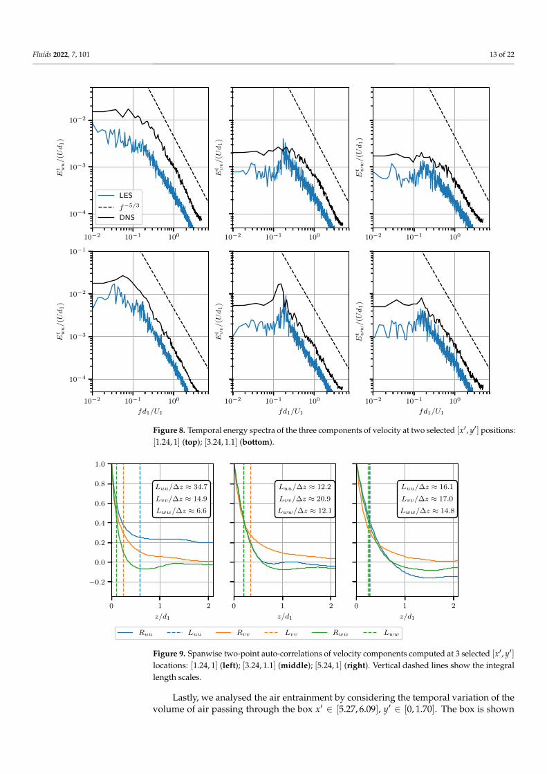
The analysis continued with the consideration of the temporal energy spectra of thevelocity fluctuations. These were computed at two [x′, y′] positions: [1.24, 1], [3.24, 1.1].These are shown with red dots in the top-left plot in Figure 3. Note that the x′ values wereessentially an outcome of the simulation, since it was not possible to know the value ofxtoe a priori. Furthermore, the intention was to use the same x and y values in the wholesimulation campaign, and the location of xtoe varied slightly from simulation to simulation.The values were therefore chosen in a conservative way to ensure that both locations wereto the right of the toe. The DNS data also provided temporal velocity spectra, including thefollowing [x′, y′] positions: [0, 1], [2, 1.1]. Both the DNS and LES data are shown in Figure 8.The LES recovered the correct slope in the inertial range, which was in most cases closeto the canonical −5/3-power spectrum. Less energy was contained in the fluctuations inthe case of the LES, but this was likely a consequence of the signals being sampled fromlocations further from the toe. Spectra for all three velocity components were predictedwith comparable precision.

Fluids 2022, 7, 101 12 of 22

0.0 0.1 0.2 0.3 0.4

urms/U1

0.0

0.5

1.0

1.5

2.0

2.5

y′

x′ = 0

LES

DNS

Interface

0.0 0.1 0.2 0.3 0.4

urms/U1

x′ = 1

0.0 0.1 0.2 0.3 0.4

urms/U1

x′ = 2

0.0 0.1 0.2 0.3 0.4

urms/U1

x′ = 3

0.0 0.1 0.2 0.3 0.4

urms/U1

x′ = 4

0.0 0.1 0.2 0.3 0.4

urms/U1

x′ = 6

0.0 0.1 0.2

vrms/U1

0.0

0.5

1.0

1.5

2.0

2.5

y′

0.0 0.1 0.2

vrms/U1

0.0 0.1 0.2

vrms/U1

0.0 0.1 0.2

vrms/U1

0.0 0.1 0.2

vrms/U1

0.0 0.1 0.2

vrms/U1

0.0 0.1 0.2

wrms/U1

0.0

0.5

1.0

1.5

2.0

2.5

y′

0.0 0.1 0.2

wrms/U1

0.0 0.1 0.2

wrms/U1

0.0 0.1 0.2

wrms/U1

0.0 0.1 0.2

wrms/U1

0.0 0.1 0.2

wrms/U1

Figure 7. The profiles of urms/U1, vrms/U1, and wrms/U1 obtained in the benchmark simulation.The magenta line shows the location of the interface.

Next, the spanwise autocorrelation functions of the three velocity components, Ruiui ,were considered. These were computed at the same two [x′, y′] locations as the temporalspectra, plus an additional location further downstream: [5.24, 1]; see the black dot inFigure 3. The result is shown in Figure 9. Evidently, Ruu, did not decline to zero fortwo of the three considered locations. This indicates that the spanwise dimension of thecomputational domain was somewhat insufficient and prompted the use of a larger domainfor the simulations on the ∆x3 and ∆x4 meshes. The figure also presents the ratio of theintegral length scales Luiui and the cell size in the spanwise direction ∆z. The smallestscale to be discretised was Lww, and at [1.24, 1], it was only covered by ≈ 6.6 cells. Bycomparison, in [33], eight cells were recommended for a coarse LES. This may indicatethat even with the ∆x1 mesh, some turbulent scales were resolved poorly. Alternatively,the integral length scale may be a poor metric to relate the grid resolution for this particularflow. In any case, further downstream, Luiui grew, meaning that the resolution with respectto them improved.

Fluids 2022, 7, 101 13 of 22

10−2 10−1 100

10−4

10−3

10−2

Et uu/(Ud

1)

LES

f−5/3

DNS

10−2 10−1 100

Et vv/(Ud

1)

10−2 10−1 100

Et ww/(Ud

1)

10−2 10−1 100

fd1/U1

10−4

10−3

10−2

10−1

Et uu/(Ud

1)

10−2 10−1 100

fd1/U1

Et vv/(Ud

1)

10−2 10−1 100

fd1/U1

Et ww/(Ud

1)

Figure 8. Temporal energy spectra of the three components of velocity at two selected [x′, y′] positions:[1.24, 1] (top); [3.24, 1.1] (bottom).

0 1 2

z/d1

−0.2

0.0

0.2

0.4

0.6

0.8

1.0

Luu/∆z ≈ 34.7

Lvv/∆z ≈ 14.9

Lww/∆z ≈ 6.6

Ruu Luu Rvv Lvv Rww Lww

0 1 2

z/d1

Luu/∆z ≈ 12.2

Lvv/∆z ≈ 20.9

Lww/∆z ≈ 12.1

0 1 2

z/d1

Luu/∆z ≈ 16.1

Lvv/∆z ≈ 17.0

Lww/∆z ≈ 14.8

Figure 9. Spanwise two-point auto-correlations of velocity components computed at 3 selected [x′, y′]locations: [1.24, 1] (left); [3.24, 1.1] (middle); [5.24, 1] (right). Vertical dashed lines show the integrallength scales.

Lastly, we analysed the air entrainment by considering the temporal variation of thevolume of air passing through the box x′ ∈ [5.27, 6.09], y′ ∈ [0, 1.70]. The box is shown

Fluids 2022, 7, 101 14 of 22

with red lines in the top-left plot in Figure 3. Similar to the analysis made for the DNS [4],we considered the autocorrelation function of the recorded signal. The result is shown inFigure 10. As expected, strong periodicity was revealed. The DNS data appeared somewhatunconverged, but the location of the first peak was relatively close to the LES. The integraltime scales corresponding to the two curves were clearly different, but that is explained bythe fact that the width of the box used for sampling the signal was larger in the LES.

0 2 4 6 8 10 12 14

∆tU/d1

−0.4

−0.2

0.0

0.2

0.4

0.6

0.8

1.0

LES

DNS

Figure 10. Autocorrelation function of the time signal of the air volume passing through the boxx′ ∈ [5.27, 6.09], y′ ∈ [0, 1.70].

The primary conclusion of this section is that OpenFOAM® can be successfully usedfor scale-resolving simulations of the CHJ. This can probably be extended to include othercodes based on the same discretisation and multiphase modelling frameworks. In spiteof the slight differences in the simulation setup, the observed overall agreement with theDNS data was good not only for the first- and second-order statistical moments of theconsidered flow variables, but also for temporal turbulent spectra and the air entrainmentproperties. This justifies using the produced dataset as an accurate reference for theparticular simulation setup selected.

4.3. Influence of Modelling Parameters

In this section, the effects of the grid resolution, amount of upwinding, and interface-capturing method on the cost and accuracy of the results are considered. The cost of thesimulations is analysed first, and the associated metric, Nh, is defined as follows. First,the simulation logs were used to compute the number of physical hours necessary toadvance each simulation by 1 s. Since the simulations on different grids were parallelisedusing different amounts of computational cores, the obtained timings were then multi-plied by the corresponding amount of cores used. This assumed linear scaling of thecomputational effort with parallelisation, which was not exact, but provided a very goodapproximation in the range of core numbers used in the study. Recall also that in thesimulations using isoAdvector, the time step was adjusted to ensure the maximum Courantnumber was < 0.5, whereas 0.75 was used in the MULES simulations. To be able to accountfor the cost difference associated with the VoF algorithm as such, the cost metric for theMULES simulations was premultiplied by 0.75/0.5. Note that since a typical desktopcomputer has around 10 computational cores and the full simulation needs to be run forabout 10 s, Nh also gives a rough estimate of how many hours it would take to perform agiven simulation on a desktop machine.

The obtained values of Nh are shown in Table 2. Each entry contains two numbers,corresponding to MULES and isoAdvector. It is evident that the isoAdvector simulationsare more expensive. Depending on the other simulation parameters, the ratio of Nh variedwithin ≈ [1.17, 1.55]. As a general trend, isoAdvector became relatively more expensive

Fluids 2022, 7, 101 15 of 22

with increased mesh resolution. Numerical dissipation sometimes favourably affectedthe amount of iterations necessary to solve the pressure equation. Here, this effect wasobserved when the transition from 10% to 25% upwinding occurred, with the formeralways leading to a more expensive simulation. However, for higher u%, the effect ofdissipation on Nh was neither particularly strong nor regular. Considering the cost as afunction of ∆x, it is crucial to recall that the ∆x2 simulations were performed on a thinnerdomain. Since the computational effort did not scale linearly with the number of cells, thiscould not be directly accounted for in the metric. Based on the data, on a desktop machine,it was possible to perform ∆x4 simulations in about 3 d and ∆x3 in about 10 d. For ∆x2,the corresponding number was from 25 d to 35 d depending on the simulation settings.Taking into account the increased access of both academia and industry to HPC hardware,it can be said that the simulations on all three grids were relatively inexpensive, at least byLES standards.

Table 2. The simulation cost metric, Nh. For each ∆x and u% combination, two values are given,corresponding to MULES and isoAdvector, respectively.

u10% u25% u50% u100%

∆x2 595/825 553/855 554/778 591/801∆x3 284/- 197/257 199/264 198/250∆x4 75/- 53/62 52/66 50/64

Next, the computed profiles of 〈α〉 were investigated; see Figure 11. The benchmarksimulation revealed that the region of the flow that was most difficult to predict was di-rectly downstream of the toe. Therefore, here, we focused on the following streamwisepositions: x′ = 0.5, 1.0, 2.0. The clear trend overarching all x′ and ∆x was that a higheramount of upwinding led to better results. For the majority of ∆x and streamwise positions,using isoAdvector and u100% led to the best predictive accuracy. The fact that using moredissipative schemes improved the results was somewhat unexpected, because typically,the recommendation for scale-resolving simulations is to keep dissipativity to a minimum.However, it should be appreciated that in VoF, any parasitic currents arising due to numeri-cal errors of the dispersive type propagate into errors in the advection of the interface. Itappears that avoiding these errors is more important than resolving steep velocity gradients.As expected, the quality of the results degraded with the coarsening of the mesh. The mostprecise result on ∆x2 was quite close to the benchmark. On the coarser grids, the accuracywas acceptable considering how inexpensive the corresponding simulations were.

The predictions of the mean velocity are analysed next; see Figure 12. We focusedon the streamwise component 〈u〉 only, since the level of accuracy of 〈v〉 was similar. Itwas clear that compared to 〈α〉, the results were more robust with respect to the amountof upwinding. This is rather peculiar: the choice of interpolation scheme for u had littleeffect on 〈u〉, but a stronger effect on a different quantity, 〈α〉. Nevertheless, the profilesobtained with higher u% were generally slightly more accurate, at least in the water phase.Using isoAdvector led to superior accuracy in the gas phase, whereas in the water phase,no significant advantage over MULES was achieved. The combination of ∆x2, u100%,and isoAdvector gave the best results, which were close to the benchmark. At coarserresolutions, the accuracy deteriorated, but not as strongly as for 〈α〉.

Fluids 2022, 7, 101 16 of 22

1.00

1.25

1.50

1.75

2.00

y′ ,

∆x

2x′ = 0.5

u10%, isoAdvector

u25%, isoAdvector

u50%, isoAdvector

u100%, isoAdvector

u10%, MULES

u25%, MULES

u50%, MULES

u100%, MULES

Benchmark

x′ = 1.0 x′ = 2.0

1.00

1.25

1.50

1.75

2.00

y′ ,

∆x

3

0.0 0.5 1.0

〈αg〉

1.00

1.25

1.50

1.75

2.00

y′ ,

∆x

4

0.0 0.5 1.0

〈αg〉0.0 0.5 1.0

〈αg〉

Figure 11. The profiles of 〈α〉 obtained in the simulation campaign.

Figure 13 shows the obtained profiles of 〈k〉. The observed error patterns were sig-nificantly less regular than in 〈u〉 and 〈α〉. Two factors contributed to this. One is that 〈k〉lumped together the errors in the variances of the three velocity components. The otherwas that parasitic oscillations had a direct amplifying effect on 〈k〉. Both of the above canlead to either error cancellation or amplification. On the ∆x2 grid, the best results wereachieved with isoAdvector and 25/50% upwinding. In the case of u100%, the main peak inthe detached shear layer was somewhat under-predicted, but the discrepancy was not verysignificant. An interesting observation is that at lower grid resolutions, a secondary peakin 〈k〉 was developed for x′ = 1.0 and 2.0 right underneath the interface. This unphysicalpeak was more pronounced when isoAdvector was used and could even be observed onthe ∆x2 grid when this interface-capturing technique was used. It was present in all threecomponents of the velocity variance, although for the streamwise component, it was lesspronounced. The size of the peak grew with a decreasing amount of upwinding, whichconfirmed its numerical origin. Even apart from this additional peak, the results for 〈k〉on ∆x3 and ∆x4 were quite inaccurate, although the combination ∆x4, u50%, and MULESreproduced the main features of the benchmark profiles fairly faithfully.

Fluids 2022, 7, 101 17 of 22

1.00

1.25

1.50

1.75

2.00

y′ ,

∆x

2x′ = 0.5

u10%, isoAdvector

u25%, isoAdvector

u50%, isoAdvector

u100%, isoAdvector

u10%, MULES

u25%, MULES

u50%, MULES

u100%, MULES

Benchmark

Interface

x′ = 1.0 x′ = 2.0

1.00

1.25

1.50

1.75

2.00

y′ ,

∆x

3

0.0 0.5 1.0

〈u〉/U1

1.00

1.25

1.50

1.75

2.00

y′ ,

∆x

4

0.0 0.5 1.0

〈u〉/U1

0.0 0.5 1.0

〈u〉/U1

Figure 12. The profiles of 〈u〉/U1 obtained in the simulation campaign.

The analysis of the velocity predictions is now concluded by considering the spanwiseenergy spectra of the streamwise velocity; see Figure 14. The spectra were computed atthe same three [x, y] locations as the spanwise autocorrelation functions for the benchmarksimulations. This entailed that the respective x′ values were slightly different from simula-tion to simulation. The reason for considering spanwise spectra instead of temporal wasthat, due to a larger amount of samples to average across, the spanwise spectra were muchsmoother, making it easier to distinguish the profiles from different simulations in the plots.Unsurprisingly, increased upwinding led to heavier dampening of the high-frequencyfluctuations. Due to the log–log scale being used, it was actually difficult to distinguish anyeffects of the VoF algorithm or ∆x, besides the fact that the frequency band of the spectrumwas larger for denser meshes. One could say that for small amounts of u%, the spectrumwas relatively well predicted even at ∆x4. Therefore, one should exercise caution whenmaking judgements regarding the mesh resolution based on the spectrum predictions.

Fluids 2022, 7, 101 18 of 22

1.0

1.2

1.4

1.6

1.8

2.0

y′ ,

∆x

2x′ = 0.5

u10%, isoAdvector

u25%, isoAdvector

u50%, isoAdvector

u100%, isoAdvector

u10%, MULES

u25%, MULES

u50%, MULES

u100%, MULES

Benchmark

Interface

x′ = 1.0 x′ = 2.0

1.0

1.2

1.4

1.6

1.8

2.0

y′ ,

∆x

3

0.00 0.01 0.02

〈k〉/U21

1.0

1.2

1.4

1.6

1.8

2.0

y′ ,

∆x

4

0.00 0.01 0.02

〈k〉/U21

0.000 0.005 0.010 0.015

〈k〉/U21

Figure 13. The profiles of 〈k〉/U21 obtained in the simulation campaign.

Finally, the periodicity of air entrainment was analysed. As for the benchmark sim-ulation, the autocorrelation functions of the volume of air passing through a box locatedsome distance downstream of the toe (see the top-left plot in Figure 3) were computed. Theresults are shown in Figure 15. For ∆x2 and ∆x3, the location of the first peak was quite wellpredicted by all the simulations, whereas for ∆x4, the accuracy deteriorated, in particularfor some of the simulations using MULES. Animations of the α = 0.5 isosurface revealedthat isoAdvector did a much better job at preserving the sharpness of the interface as theentrained bubbles travelled downstream. Therefore, if tracking the fate of the bubbles isimportant, using this VoF approach is recommended. It should also be noted that while allthe simulation predicted similar entrainment frequencies, other statistical air entrainmentproperties did not agree equally well. For example, the mean amount of air within themonitored box was highly affected by the choice of the VoF method, with MULES givingsystematically higher values.

Fluids 2022, 7, 101 19 of 22

10−5

10−3

10−1

Ez uu/(d

1U

1),

∆x

2

u10%, isoAdvector

u25%, isoAdvector

u50%, isoAdvector

u100%, isoAdvector

u10%, MULES

u25%, MULES

u50%, MULES

u100%, MULES

Benchmark

−5/3 slope

10−5

10−3

10−1

Ez uu/(d

1U

1),

∆x

3

100 101 102

kzd1

10−5

10−3

10−1

Ez uu/(d

1U

1),

∆x

4

100 101 102

kzd1

100 101 102

kzd1

Figure 14. The spanwise velocity spectra obtained in the simulations at three selected locations:[1.24, 1] (left); [3.24, 1.1] (middle); [5.24, 1.4] (right).

0 5 10

∆tU/d1

−0.4

−0.2

0.0

0.2

0.4

0.6

0.8

1.0∆x2

u10%, isoAdvector

u25%, isoAdvector

u50%, isoAdvector

u100%, isoAdvector

u10%, MULES

u25%, MULES

u50%, MULES

u100%, MULES

Benchmark

0 5 10

∆tU/d1

−0.4

−0.2

0.0

0.2

0.4

0.6

0.8

1.0∆x3

0 5 10

∆tU/d1

−0.4

−0.2

0.0

0.2

0.4

0.6

0.8

1.0∆x4

Figure 15. The obtained autocorrelation functions of the volume of leaked air.

5. Conclusions

This article presented the results from an extensive simulation campaign studying theeffects of different modelling parameters on the accuracy of LES of CHJ flow at Fr1 = 2.

Fluids 2022, 7, 101 20 of 22

The simulations were performed with a general-purpose finite-volume-based CFD code,making the obtained results relevant for industry professionals and researches alike.

A benchmark simulation on a dense grid was conducted to test whether commonlyemployed VoF-based multiphase modelling methodologies are sufficiently accurate tocapture the complicated physics of the flow. The comparison with the DNS data [4] showedthat the answer was positive, and good agreement with the reference was found for theconsidered quantities of interest. However, it was also revealed that numerical instabilities,discussed in Section 2.5, constituted a significant problem. It was virtually impossible toknow a priori whether the chosen numerical setup would lead to a stable simulation, and acrash may occur sporadically after a significant part of the simulation time has already past.Addressing the primary sources of instability (surface tension, density gradient term in (1))should therefore be a high priority for the development of VoF solvers in OpenFOAM®

and other codes based on similar algorithms.The rest of the simulation campaign focused on the effects of the grid resolution, amount

of upwinding, and VoF methodology. One of the most interesting results was that the mostdissipative scheme, u100%, led to the best results for nearly all the considered quantities ofinterest. This represents another example of how multiphase simulations can react counter-intuitively with respect to a change in the computational algorithm. It appeared that, for volumefraction transfer, ensuring the lack of strong dispersive errors was for this case more importantthan minimizing the numerical dissipation. Fortunately, dissipation also favours stability, whichmeans that having both an accurate and stable numerical setup is possible.

Using the geometric VoF methodology, isoAdvector, led to improved interface sharpnessand thus improved the resolution of entrained bubbles. The improvement in the accuracy ofaveraged flow quantities compared to MULES was however, not so strong, and for selectedquantities and streamwise locations, MULES actually gave better results. The chance of insta-bility was also increased by isoAdvector, and for some combinations of modelling parameters,the simulations could not be run. Unfortunately, this included the benchmark simulation. Thecomputational costs of isoAdvector simulations were also significantly larger than their MULEScounterparts; see Table 2. For equivalent simulation settings, the maximum cost ratio was 1.5;however, due to MULES being more stable, it is possible to select a larger time step, whichwould make the difference even larger. It is thus recommended to use isoAdvector whentracking the fate of individual air bubbles is particularly important.

The grid resolution appeared to be the most significant factor when it came to thepredictive accuracy. The sensitivity was particularly strong right downstream of the toe,for which even the ∆x2 grid gave relatively poor results. However, further downstream,the loss of accuracy quickly decreased. The ∆x3 grid could be used to reduce the costssignificantly and still maintain a level of predictive accuracy that can be suitable forindustrial simulations. Using the ∆x4 can only be recommended when the CHJ is a part ofa larger flow configuration and is not of particular interest as such.

Author Contributions: Conceptualisation, T.M., S.K.A. and R.E.B.; methodology, T.M. and S.K.A.;investigation, T.M. and S.K.A.; resources, S.K.A. and R.E.B.; writing—original draft preparation, T.M.;writing—review and editing, S.K.A. and R.E.B.; visualisation, T.M.; supervision, R.E.B.; fundingacquisition, R.E.B; project administration, R.E.B. All authors have read and agreed to the publishedversion of the manuscript.

Funding: This work was supported by Grant Number P38284-2 from the Swedish Energy Agency.

Institutional Review Board Statement: Not applicable.

Informed Consent Statement: Not applicable.

Data Availability Statement: The data presented in this study are openly available on Figshare athttps://doi.org/10.6084/m9.figshare.12593480.v5 (accessed on 30 January 2022).

Acknowledgments: The simulations were performed on resources provided by Chalmers Centre forComputational Science and Engineering (C3SE) and UNINETT Sigma2—the National Infrastructure

Fluids 2022, 7, 101 21 of 22

for High Performance Computing and Data Storage in Norway. The authors are thankful to MiladMortazavi for sharing the data files from the DNS [4].

Conflicts of Interest: The authors declare no conflict of interest.

Appendix A. Effect of Explicit Subgrid-Scale Modelling

To test the effect of the explicit modelling of subgrid scales, a simulation using theWALE model was conducted. The ∆x3 grid was used and 10% upwinding, the latterin order to minimise the relative weight of the numerical dissipation compared to thedissipation introduced by the model.

The obtained results are shown in Figure A1. Clearly, the effect of the SGS model wasmarginal, both on the air concentration and streamwise velocity.

0.00 0.25 0.50 0.75 1.00

〈αg〉

1.00

1.25

1.50

1.75

2.00

2.25

2.50

2.75

3.00

y/d

1

0.00 0.25 0.50 0.75 1.00

〈u〉/U1

0

1

2

3

4

5

6

7

8

y/d

1

x = 0 No model

x = 0 WALE

x = 1 No model

x = 1 WALE

x = 2 No model

x = 2 WALE

x = 3 No model

x = 3 WALE

Figure A1. Effect of explicit SGS modelling using the WALE model. Profiles of the volume fraction ofair (left) and streamwise velocity (right).

References1. Bayon-Barrachina, A.; Lopez-Jimenez, P.A. Numerical analysis of hydraulic jumps using OpenFOAM. J. Hydroinform. 2015,

17, 662–678. [CrossRef]2. Valero, D.; Viti, N.; Gualtieri, C. Numerical simulation of hydraulic jumps. Part 1: Experimental data for modelling performance

assessment. Water 2018, 11, 36. [CrossRef]3. Valero, D.; Viti, N.; Gualtieri, C. Numerical simulation of hydraulic jumps. Part 2: Recent results and future outlook. Water 2018,

11, 28. [CrossRef]4. Mortazavi, M.; Le Chenadec, V.; Moin, P.; Mani, A. Direct numerical simulation of a turbulent hydraulic jump: Turbulence

statistics and air entrainment. J. Fluid Mech. 2016, 797, 60–94. [CrossRef]5. Chanson, H. The Hydraulics of Open Channel Flow: An Introduction; Elsevier: Burlington, MA, USA, 2004; p. 601.6. Jain, S.C. Open-Channel Flow; Wiley: Hoboken, NJ, USA, 2001; p. 328.7. Kundu, P.K.; Cohen, I.M. Fluid Mechanics, 4th ed.; Academic Press: Burlington, MA, USA, 2008.8. Retsinis, E.; Papanicolaou, P. Numerical and experimental study of classical hydraulic jump. Water 2020, 12, 1766. https://

doi.org/10.3390/w12061766. [CrossRef]9. Ma, J.; Oberai, A.A.; Lahey, R.; Drew, D.A. Modeling air entrainment and transport in a hydraulic jump using two-fluid RANS

and DES turbulence models. Heat Mass Transf. 2011, 47, 911–919. [CrossRef]10. Jesudhas, V.; Balachandar, R.; Roussinova, V.; Barron, R. Turbulence characteristics of classical hydraulic jump using DES. J.

Hydraul. Eng. 2018, 144, 04018022. [CrossRef]11. Jesudhas, V.; Balachandar, R.; Wang, H.; Murzyn, F. Modelling hydraulic jumps: IDDES versus experiments. Environ. Fluid Mech.

2020, 20, 393–413. [CrossRef]12. Gonzalez, A.; Bombardelli, F.A. Two-phase-flow theoretical and numerical models for hydraulic jumps, including air entrainment.

In Proceedings of the 31st IAHR Congress, Seoul, South Korea, 11–16 September 2005.13. Lubin, P.; Glockner, S.; Chanson, H. Numerical simulation of air entrainment and turbulence in a hydraulic jump. In Proceedings

of the Colloque SHF: Modeles Physiques Hydrauliques, Lyon, France, 24–25 November 2009; pp. 109–114.

Fluids 2022, 7, 101 22 of 22

14. Hirt, C.W.; Nichols, B.D. Volume of Fluid (VOF) method for the dynamics of free boundaries. J. Comput. Phys. 1981, 39, 201–225.[CrossRef]

15. Brackbill, J.U.; Kothe, D.B.; Zemach, C. A continuum method for modeling surface tension. J. Comput. Phys. 1992, 100, 335–354.[CrossRef]

16. Damián, S.M. An Extended Mixture Model for the Simultaneous Treatment of Short and Long Scale Interfaces. Ph.D. Thesis,National University of the Littoral, Santa Fe, Argentina, 2013.

17. Zalesak, S.T. Fully multidimensional flux-corrected transport algorithms for fluids. J. Comput. Phys. 1979, 31, 335–362. [CrossRef]18. Roenby, J.; Bredmose, H.; Jasak, H. A computational method for sharp interface advection. R. Soc. Open Sci. 2016, 3. [CrossRef]

[PubMed]19. Issa, R.I. Solution of the implicitly discretised fluid flow equations by operator-splitting. J. Comput. Phys. 1986, 62, 40–65.

[CrossRef]20. Rusche, H. Computational Fluid Dynamics of Dispersed Two-Phase Flows at High Phase Fractions. Ph.D. Thesis, Imperial

College of Science, Technology and Medicine, London, UK, 2002.21. Versteeg, H.K.; Malalasekera, W. An Introduction to Computational Fluid Dynamics: The Finite Volume Method, 2nd ed.; Pearson

Education Limited, Essex, England, 2007.22. Nicoud, F.; Ducros, F. Subgrid-scale stress modelling based on the square of the velocity gradient tensor. Flow Turbul. Combust.

1999, 62, 183–200.:1009995426001. [CrossRef]23. Mukha, T. Inflow Generation for Scale-Resolving Simulations of Turbulent Boundary Layers; Uppsala University: Uppsala, Sweden,

2016.24. Cano-Lozano, J.C.; Bolaños-Jiménez, R.; Gutiérrez-Montes, C.; Martínez-Bazán, C. The use of Volume of Fluid technique to

analyze multiphase flows: Specific case of bubble rising in still liquids. Appl. Math. Model. 2015, 39, 3290–3305. [CrossRef]25. Scheufler, H. Implementation of new surface tension models for the Volume of Fluid Method. In Proceedings of the 7th ESI

OpenFOAM Conference, Berlin, Germany, 15–17 October 2019.26. Popinet, S. An accurate adaptive solver for surface-tension-driven interfacial flows. J. Comput. Phys. 2009, 228, 5838–5866.

[CrossRef]27. Gamet, L.; Scala, M.; Roenby, J.; Scheufler, H.; Pierson, J.L. Validation of volume-of-fluid OpenFOAM® isoAdvector solvers using

single bubble benchmarks. Comput. Fluids 2020, 213, 104722. [CrossRef]28. Scheufler, H.; Roenby, J. TwoPhaseFlow: An OpenFOAM based framework for development of two phase flow solvers. arXiv

2021, arXiv:2103.00870.29. Vukcevic, V.; Jasak, H.; Gatin, I. Implementation of the Ghost Fluid Method for free surface flows in polyhedral Finite Volume

framework. Comput. Fluids 2017, 153, 1–19. [CrossRef]30. Witt, A.; Gulliver, J.; Shen, L. Simulating air entrainment and vortex dynamics in a hydraulic jump. Int. J. Multiph. Flow 2015,

72, 165–180. [CrossRef]31. Witt, A.; Gulliver, J.S.; Shen, L. Numerical investigation of vorticity and bubble clustering in an air entraining hydraulic jump.

Comput. Fluids 2018, 172, 162–180. [CrossRef]32. Bayon, A.; Valero, D.; García-Bartual, R.; Vallés-Morán, F.J.; López-Jiménez, P.A. Performance assessment of OpenFOAM and

FLOW-3D in the numerical modeling of a low Reynolds number hydraulic jump. Environ. Model. Softw. 2016, 80, 322–335.[CrossRef]

33. Davidson, L. Large Eddy Simulations: How to evaluate resolution. Int. J. Heat Fluid Flow 2009, 30, 1016–1025. [CrossRef]